Neural Unbalanced Optimal Transport
via Cycle-Consistent Semi-Couplings

Abstract

Comparing unpaired samples of a distribution or population taken at different points in time is a fundamental task in many application domains where measuring populations is destructive and cannot be done repeatedly on the same sample, such as in single-cell biology. Optimal transport (OT) can solve this challenge by learning an optimal coupling of samples across distributions from unpaired data. However, the usual formulation of OT assumes conservation of mass, which is violated in unbalanced scenarios in which the population size changes (e.g., cell proliferation or death) between measurements. In this work, we introduce NubOT, a neural unbalanced OT formulation that relies on the formalism of semi-couplings to account for creation and destruction of mass. To estimate such semi-couplings and generalize out-of-sample, we derive an efficient parameterization based on neural optimal transport maps and propose a novel algorithmic scheme through a cycle-consistent training procedure. We apply our method to the challenging task of forecasting heterogeneous responses of multiple cancer cell lines to various drugs, where we observe that by accurately modeling cell proliferation and death, our method yields notable improvements over previous neural optimal transport methods.

1 Introduction

Modeling change is at the core of various problems in the natural sciences, from dynamical processes driven by natural forces to population trends induced by interventions. In all these cases, the gold standard is to track particles or individuals across time, which allows for immediate estimation of individual (or aggregate) effects. But maintaining these pairwise correspondences across interventions or time is not always possible, for example, when the same sample cannot be measured more than once. This is typical in biomedical sciences, where the process of measuring is often altering or destructive. For example, single-cell biology profiling methods destroy the cells and thus cannot be used repeatedly on the same cell. In these situations, one must rely on comparing different replicas of a population and, absent a natural identification of elements across the populations, infer these correspondences from data in order to model evolution or intervention effects.

The problem of inferring correspondences across unpaired samples in biology has been traditionally tackled by relying on average and aggregate perturbation responses (Green & Pelkmans, 2016; Zhan et al., 2019; Sheldon et al., 2007) or by applying mechanistic or linear models (Yuan et al., 2021; Dixit et al., 2016) in, potentially, a learned latent space (Lotfollahi et al., 2019). Cellular responses to treatments are, however, highly complex and heterogeneous. To effectively predict the drug response of a patient during treatment and capture such cellular heterogeneity, it is necessary to learn nonlinear maps describing such perturbation responses on the level of single cells. Assuming perturbations incrementally alter molecular profiles of cells, such as gene expression or signaling activities, recent approaches have utilized optimal transport to predict changes and alignments (Schiebinger et al., 2019; Bunne et al., 2022a; Tong et al., 2020). By returning a coupling between control and perturbed cell states, which overall minimizes the cost of matching, optimal transport can solve that puzzle and reconstruct these incremental changes in cell states over time.

Despite the advantages mentioned above, the classic formulation of OT is ill-suited to model processes where the population changes in size, e.g., where elements might be created or destroyed over time. This is the case, for example, in single-cell biology, where interventions of interest typically promote proliferation of certain cells and death of others. Such scenarios violate the assumption of conservation of mass that the classic OT problem relies upon. Relaxing this assumption yields a generalized formulation, known as the unbalanced OT (UBOT) problem, for which recent work has studied its properties (Liero et al., 2018; Chizat et al., 2018a), numerical solution (Chapel et al., 2021), and has applied it successfully to problems in single cell biology (Yang & Uhler, 2019). Yet, these methods typically scale poorly with sample size, are prone to unstable solutions, or make limiting assumptions, e.g., only allowing for destruction but not creation of mass.

In this work, we address these shortcomings by introducing a novel formulation of the unbalanced OT problem that relies on the formalism of semi-couplings introduced by Chizat et al. (2018b), while still obtaining an explicit transport map that models the transformation between distributions. The advantage of the latter is that it allows mapping new out-of-sample points, and it provides an interpretable characterization of the underlying change in distribution. Since the unbalanced OT problem does not directly admit a Monge (i.e., mapping-based) formulation, we propose to learn to jointly ‘re-balance’ the two distributions, thereby allowing us to estimate a map between their rescaled versions. To do so, we leverage prior work (Makkuva et al., 2020; Korotin et al., 2021) that learns the transport map as the gradient of a convex dual potential (Brenier, 1987) parameterized via an input convex neural network (Amos et al., 2017). In addition, we derive a simple update rule to learn the rescaling functions. Put together, these components yield a reversible, parameterized, and computationally feasible implementation of the semi-coupling unbalanced OT formulation (Fig.  1).

In short, the main contributions of this work are: (i) A novel formulation of the unbalanced optimal transport problem that weaves together the theoretical foundations of semi-couplings with the practical advantage of transport maps; (ii) A general, scalable, and efficient algorithmic implementation for this formulation based on dual potentials parameterized via convex neural network architectures; and (iii) An empirical validation on the challenging task of predicting perturbation responses of single cells to multiple cancer drugs, where our method successfully predicts cell proliferation and death, in addition to faithfully modeling the perturbation responses on the level of single cells.

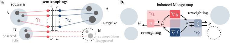
Figure 1: a. A semi-coupling pair ( $\gamma_{1}$, $\gamma_{2}$) consists of two couplings that together solve the unbalanced OT problem. Intuitively, $\gamma_{1}$ describes where mass goes as it leaves from $\mu$, and $\gamma_{2}$ where it comes from as it arrives in $\nu$. b. NubOT parameterizes the semi-couplings ( $\gamma_{1}$, $\gamma_{2}$) as the composition of reweighting functions $\eta$ and $\zeta$ and the dual potentials $f$ and $g$ between the then balanced problem.

2 Background

2.1 Optimal Transport

For two probability measures $\mu,\nu$ in $\mathcal{P}(\mathcal{X})$ with $\mathcal{X}=\mathbb{R}^{d}$ and a real-valued continuous cost function $c\in\mathcal{C}(\mathcal{X}^{2})$, the optimal transport problem (Kantorovich, 1942) is defined as

$$\textup{OT}(\mu,\nu)\vcentcolon=\inf_{\gamma\in\Gamma(\mu,\nu)}\int_{{\mathcal{X}}^{2}}c(x,y)\gamma(dx,dy),$$ (1)

where $\Gamma(\mu,\nu)=\{\gamma\in{\mathcal{M}}_{+}({\mathcal{X}}^{2}),\text{ s.t. }(\operatorname{Proj}_{1})_{\sharp}\gamma=\mu,(\operatorname{Proj}_{2})_{\sharp}\gamma=\nu\}$ is the set of couplings in the cone of nonnegative Radon measures ${\mathcal{M}}_{+}({\mathcal{X}}^{2})$ with respective marginals $\mu,\nu$. When instantiated on finite discrete measures, such as $\mu=\sum_{i=1}^{n}u_{i}\delta_{{\mathbf{x}}_{i}}$ and $\nu=\sum_{j=1}^{m}v_{j}\delta_{{\mathbf{y}}_{j}}$, with $\mathbf{u}\in\Sigma_{n},\mathbf{v}\in\Sigma_{m}$ this problem translates to a linear program, which can be regularized using an entropy term (Peyré & Cuturi, 2019). For $\varepsilon\geq 0$, set

$$\textup{OT}_{\varepsilon}(\mu,\nu)\vcentcolon=\min_{\mathbf{P}\in U({\mathbf{u}},{\mathbf{v}})}\langle\mathbf{P},[c({\mathbf{x}}_{i},{\mathbf{y}}_{j})]_{ij}\rangle\,-\varepsilon H(\mathbf{P}),$$ (2)

where $H(\mathbf{P})\vcentcolon=-\sum_{ij}\mathbf{P}_{ij}(\log\mathbf{P}_{ij}-1)$ and the polytope $U({\mathbf{u}},{\mathbf{v}})$ is the set of matrices $\{\mathbf{P}\in\mathbb{R}^{n\times m}_{+},\mathbf{P}\mathbf{1}_{m}={\mathbf{u}},\mathbf{P}^{\top}\mathbf{1}_{n}={\mathbf{v}}\}$. For clarity, we will sometimes write $\textup{OT}_{\varepsilon}({\mathbf{u}},{\mathbf{v}},\{{\mathbf{x}}_{i}\},\{{\mathbf{y}}_{j}\})$. Notice that the definition above reduces to (1) when $\varepsilon=0$. Setting $\varepsilon>0$ yields a faster and differentiable proxy to approximate OT and allows fast numerical approximation via the Sinkhorn algorithm (Cuturi, 2013), but introduces a bias, since in general $\textup{OT}_{\varepsilon}(\mu,\mu)\neq 0$.

Neural optimal transport.

To parameterize (1) and allow to predict how a measure evolves from $\mu$ to $\nu$, we introduce an alternative formulation known as the Monge problem (1781) given by

$$\textup{OT}_{\varepsilon}(\mu,\nu)=\inf_{T:T_{\sharp}\mu=\nu}\int_{\mathcal{X}}c(x,T(x))d\mu(x),$$ (3)

with pushforward operator $\sharp$ and the optimal solution $T^{*}$ known as the Monge map between $\mu$ and $\nu$. When cost $c$ is the quadratic Euclidean distance, i.e., $c=\|\cdot\|^{2}_{2}$, Brenier’s theorem (1987) states that this Monge map is necessarily the gradient $\nabla\psi$ of a convex potential $\psi:\mathcal{X}\mapsto\mathbb{R}$ such that $\nabla\psi_{\sharp}\mu=\nu$, i.e., $T^{*}(x)=\nabla\psi(x)$. This connection has far-reaching impact and is a central component of recent neural optimal transport solvers (Makkuva et al., 2020; Bunne et al., 2022c; Alvarez-Melis et al., 2022; Korotin et al., 2020; Bunne et al., 2022b; Fan et al., 2021b). Instead of (indirectly) learning the Monge map $T$ (Yang & Uhler, 2019; Fan et al., 2021a), it is sufficient to restrict the computational effort to learning a good convex potential $\nabla_{\theta}$, parameterized via input convex neural networks (ICNN) (Amos et al., 2017), s.t. $\nabla_{\theta}\psi\sharp\mu=\nu$. Alternatively, parameterizations of such maps can be carried out via the dual formulation of (1) (Santambrogio, 2015, Proposition 1.11, Theorem 1.39), i.e.,

$$\textup{OT}(\mu,\nu)\vcentcolon=\sup_{\begin{subarray}{c}f,g\in\mathcal{C}(\mathcal{X})\\ f\oplus g\leq c\end{subarray}}\int fd\mu+\int gd\nu,$$ (4)

where the dual potentials $f,g$ are continuous functions from $\mathcal{X}$ to $\mathbb{R}$, and $f\oplus g\mapsto f(x)+g(x)$. Based on Brenier (1987), Makkuva et al. (2020) derive an approximate min-max optimization scheme parameterizing the duals $f,g$ via two convex functions. The objective thereby reads

$$\textup{OT}_{\text{n}}(\mu,\nu)=\sup_{f\text{ convex}}\mathop{\mathrm{inf}\vphantom{\mathrm{sup}}}_{g\text{ convex}}\underbrace{\frac{1}{2}\mathbb{E}\left[\|x\|+\|y\|\right]}_{\mathcal{C}_{\mu,\nu}}-\underbrace{\mathbb{E}_{\mu}[f(x)]-\mathbb{E}_{\nu}[\langle y,\nabla g(y)\rangle-f(\nabla g(y))]}_{\mathcal{V}_{\mu,\nu}(f,g)}.$$ (5)

When paramterizing $f$ and $g$ via a pair of ICNNs with parameters $\theta_{f}$ and $\theta_{g}$, this neural OT scheme then allows to predict $\nu$ or $\mu$ via $\nabla g_{\theta_{g}\sharp}\mu$ or $\nabla f_{\theta_{f}\sharp}\nu$, respectively. We further discuss neural primal (Fan et al., 2021a; Yang & Uhler, 2019) and dual approaches (Makkuva et al., 2020; Korotin et al., 2020; Bunne et al., 2021) in §D.2.

2.2 Unbalanced optimal transport.

A major constraint of problem (1) is its restriction to a pair of probability distributions $\mu$ and $\nu$ of equal mass. Unbalanced optimal transport (Benamou, 2003; Liero et al., 2018; Chizat et al., 2018b) lifts this requirement and allows a comparison between unnormalized measures, i.e., via

$$\inf_{\gamma\in\mathcal{M}_{+}({\mathcal{X}}^{2})}\int_{{\mathcal{X}}^{2}}c(x,y)\gamma(dx,dy)+\tau_{1}\mathcal{D}_{f_{1}}((\operatorname{Proj}_{1})_{\sharp}\gamma\mid\mu)+\tau_{2}\mathcal{D}_{f_{2}}((\operatorname{Proj}_{2})_{\sharp}\gamma\mid\nu),$$ (6)

with $f$-divergences $D_{f_{1}}$ and $D_{f_{2}}$ induced by $f_{1},f_{2}$, and parameters $(\tau_{1},\tau_{2})$ controlling how much mass variations are penalized as opposed to transportation of the mass. When introducing an entropy regularization as in (2), the unbalanced OT problem between discrete measures ${\mathbf{u}}$ and ${\mathbf{v}}$, i.e.,

$$\textup{UBOT}({\mathbf{u}},{\mathbf{v}})\vcentcolon=\min_{\Gamma\in\mathbb{R}_{+}^{n\times m}}\langle\Gamma,[c(x_{i},y_{j})]_{ij}\rangle+\tau_{1}{\mathcal{D}}_{f_{1}}(\Gamma\mathds{1}_{m}\mid{\mathbf{u}})+\tau_{2}{\mathcal{D}}_{f_{2}}(\Gamma^{\top}\mathds{1}_{m}\mid{\mathbf{v}})\,-\varepsilon H(\Gamma),$$ (7)

can be efficiently solved via generalizations of the Sinkhorn algorithm (Chizat et al., 2018a; Cuturi, 2013; Benamou et al., 2015) . We describe alternative formulations of the unbalanced OT problem in detail, review recent applications, and provide a broader literature review in the Appendix (§A.1).

3 A Neural Unbalanced Optimal Transport Model

The method we propose weaves together a rigorous formulation of the unbalanced optimal transport problem based on semi-couplings (introduced below) with a practical and scalable OT mapping estimation method based on input convex neural network parameterization of the dual OT problem.

Semi-coupling formulation.

Chizat et al. (2018b) introduced a class of distances that generalize optimal transport for the unbalanced setting. They introduce equivalent dynamic and static formulations of the problem, the latter of which relies on semi-couplings to allow for variations of mass. These are generalizations of couplings whereby only one of the projections coincides with a prescribed measure. Formally, the set of semi-couplings between measures $\mu$ and $\nu$ is defined as

$$\Gamma\left(\mu,\nu\right)\stackrel{{\scriptstyle\text{ def. }}}{{=}}\left\{\left(\gamma_{0},\gamma_{1}\right)\in\left(\mathcal{M}_{+}\left({\mathcal{X}}^{2}\right)\right)^{2}:\left(\operatorname{Proj}_{1}\right)_{\sharp}\gamma_{0}=\mu,\left(\operatorname{Proj}_{2}\right)_{\sharp}\gamma_{1}=\nu\right\}.$$ (8)

With this, the unbalanced Kantorovich OT problem can be written as $C_{k}(\mu,\nu)=\inf_{(\gamma_{0},\gamma_{1})\in\Gamma\left(\mu,\nu\right)}\int c(x,\tfrac{\gamma_{0}}{\gamma},y,\tfrac{\gamma_{1}}{\gamma})\mathop{}\!\mathrm{d}\gamma(x,y)$, where $\gamma$ is any joint measure for which $\gamma_{0},\gamma_{1}\ll\gamma$.

Although this formulation lends itself to formal theoretical treatment, it has at least two limitations. First, it does not explicitly model a mapping between measures. Indeed, no analogue of the celebrated Brenier’s theorem is known for this setting. Second, deriving a computational implementation of this problem is challenging by the very nature of the semi-couplings: being undetermined along one marginal makes it hard to model the space in (8).

Rebalancing with proxy measures.

To turn the semi-coupling formulation of unbalanced OT into a computationally feasible method, we propose to conceptually break the problem into balanced and unbalanced subproblems, each tackling a different aspect of the difference between measures: feature transformation and mass rescaling. These in turn imply a decomposition of the semi-couplings of (8), as we will show later. Specifically, we seek proxy measures $\tilde{\mu}$ and $\tilde{\nu}$ with equal mass (i.e., $\mu({\mathcal{X}})=\tilde{\nu}({\mathcal{X}})$) across which to solve a balanced OT problem through a Monge/Brenier formulation. To decouple measure scaling from feature transformation, we propose to choose $\tilde{\mu}$ and $\tilde{\nu}$ simply as rescaled versions of $\mu$ and $\nu$. Thus, formally, we seek $\tilde{\mu},\tilde{\nu}\in\mathcal{M}_{+}(\mathcal{X})$ and $T,S:\mathcal{X}\rightarrow\mathcal{X}$ such that

$$\tilde{\mu}=\eta\cdot\mu,\quad\tilde{\nu}=\zeta\cdot\nu,\quad T_{\sharp}\tilde{\mu}=\tilde{\nu},\quad S_{\sharp}\tilde{\nu}=\tilde{\mu},$$ (9)

where $\eta,\zeta:{\mathcal{X}}\rightarrow\mathbb{R}^{+}$ are scalar fields, $\eta\cdot\mu$ denotes the measure with density $\eta(x)\mathop{}\!\mathrm{d}\mu(x)$ (analogously for $\zeta\cdot\nu)$, and $T,S$ are a pair of forward/backward optimal transport maps between $\tilde{\mu}$ and $\tilde{\nu}$ (Fig. 1b).

Devising an optimization scheme to find all relevant components in (9) is challenging. In particular, it involves solving an OT problem whose marginals are not fixed, but that will change as the reweighting functionals $\eta,\zeta$ are updated. We propose an alternating minimization approach, whereby we alternative solve for $\eta,\zeta$ (through an approximate scaling update) and $T,S$ (through gradient updates on ICNN convex potentials, as described in Section 2.1).

Updating rescaling functions.

Given current estimates of $\eta$ and $T$, we consider the UBOT problem (6) between $T_{\sharp}(\eta\cdot\mu)=T_{\sharp}\tilde{\mu}$ and $\nu$. Although in general these two measures will not be balanced (hence why we need to use UBOT instead of usual OT), our goal is to eventually achieve this. To formalize this, let us use the shorthand notation $\pi_{\textup{UB}}^{*}(\alpha,\beta)\stackrel{{\scriptstyle\mathclap{\mbox{def.}}}}{{=}}\operatorname*{argmin}_{\pi}\textup{UBOT}(\pi;\alpha,\beta)$, where UBOT is defined in (7). For a fixed $T$, our goal is to find $w$ such that $(\operatorname{Proj}_{1})_{\sharp}[\pi_{\textup{UB}}^{*}(T_{\sharp}(\eta\cdot\mu),\nu)]=T_{\sharp}(\eta\cdot\mu)$. For the discrete setting (finite samples), this corresponds to finding a vector $\mathbf{e}$ satisfying:

$$\sum_{j=1}^{m}[\Gamma]_{ij}=\mathbf{e}\odot\mathbf{u},\quad\text{where}\medspace\Gamma=\operatorname*{argmin}\textup{UBOT}(\mathbf{e}\odot\mathbf{u},T({\mathbf{x}}_{i}),\mathbf{v},{\mathbf{y}}_{j}).$$ (10)

For a fixed $T$, the vector ${\mathbf{e}}^{*}$ satisfying this system can be found via a fixed-point iteration. In practice, we approximate it instead with a single-step update using the solution to the unscaled problem:

$$\Gamma\leftarrow\textup{UBOT}(\mathbf{u},T({\mathbf{x}}_{i}),\mathbf{v},{\mathbf{y}}_{j});\qquad\mathbf{e}\leftarrow\Gamma\mathds{1}\oslash\mathbf{u};$$

which empirically provides a good approximation on the optimal ${\mathbf{e}}^{*}$ but is significantly more efficient. Apart from requiring a single update, whenever $\mathbf{u}$ and $\mathbf{v}$ are uniform (as in most applications where the samples are assumed to be drawn i.i.d.) solving this problem between unscaled histograms will be faster and more stable than solving its scaled (and therefore likely non-uniform) counterpart in (10).

Analogously, for a given $S$, we choose $\zeta$ that ensures $(\operatorname{Proj}_{2})_{\sharp}[\pi_{\textup{UB}}^{*}(S_{\sharp}(\zeta\cdot\nu),\mu)]=S_{\sharp}(\zeta\cdot\nu)$. For empirical measures, this yields the update:

$$\Gamma\leftarrow\textup{UBOT}(\mathbf{v},S({\mathbf{y}}_{j}),\mathbf{u},{\mathbf{x}}_{i});\qquad\mathbf{z}\leftarrow\Gamma\mathds{1}\oslash\mathbf{v};$$

In order to be able to predict mass changes for new samples, we will use the discrete $\mathbf{e},\mathbf{z}$ to fit continuous versions of $\eta,\zeta$ via functions parameterized as neural networks trained to achieve $\eta({\mathbf{x}}_{i})\approx e_{i}\medspace\forall i\in\{1,\dots,n\}$ and $\zeta({\mathbf{y}}_{j})\approx z_{j}\medspace\forall j\in\{1,\dots,m\}$.

Updating mappings.

For a fixed pair of $\eta,\zeta$, we want $T$ and $S$ to be a pair of optimal OT maps between $\tilde{\mu}$ and $\tilde{\nu}$. Since these are guaranteed to be balanced due to the argument above, we can use a usual (balanced) OT formulation to find them. In particular, we use the formulation of (Makkuva et al., 2020) to fit them. That is, $T=\nabla g$ and $S=\nabla f$ for convex potentials $f$ and $g$, parameterized as ICNNs with parameters $\theta_{f}$ and $\theta_{g}$. The corresponding objective for these two potentials is:

$$\mathcal{L}(f,g) =\operatorname*{\mathbb{E}}_{x\sim\tilde{\mu}}\left[f(\nabla g)-\langle x,\nabla g(x)\rangle\right]-\operatorname*{\mathbb{E}}_{y\sim\tilde{\nu}}\left[f(y)\right]$$

$$=\int_{\mathcal{X}}\bigl{[}f(\nabla g(x))-\langle x,\nabla g(x)\rangle\bigr{]}\eta(x)\mathop{}\!\mathrm{d}\mu(x)-\int f(y)\zeta(y)\mathop{}\!\mathrm{d}\nu(y).$$

In the finite sample setting, this objective becomes:

$$\mathcal{L}(f,g)=\frac{1}{n}\sum_{i=1}^{n}e_{i}\left[f(\nabla g({\mathbf{x}}_{i}))-\langle{\mathbf{x}}_{i},\nabla g({\mathbf{x}}_{i})\rangle\right]-\sum_{j=1}^{m}z_{j}f({\mathbf{y}}_{j}).\vspace{-0.2cm}$$ (11)

The optimization procedure is summarized in Algorithm 1.

Transforming new samples.

After learning $f,g,\eta,\zeta$, we can use these functions to transform (map and rescale) new samples, i.e., beyond those used for optimization. For a given source datapoint ${\mathbf{x}}$ with mass $u$, we transform it as $({\mathbf{x}},u)\mapsto(\nabla g({\mathbf{x}}),\eta({\mathbf{x}})\cdot u\cdot\zeta(\nabla g({\mathbf{x}}))^{-1})$. Analogously, target points can be mapped backed to the source domain using $({\mathbf{y}},v)\mapsto(\nabla f({\mathbf{y}}),\zeta({\mathbf{y}})\cdot v\cdot\eta(\nabla f({\mathbf{y}}))^{-1})$.

Recovering semi-couplings.

Let us define $\tilde{\Gamma}_{1}\stackrel{{\scriptstyle\mathclap{\mbox{def.}}}}{{=}}\textup{diag}({\mathbf{e}}^{-1})^{\top}\Gamma_{1}$ and $\tilde{\Gamma}_{2}\stackrel{{\scriptstyle\mathclap{\mbox{def.}}}}{{=}}\textup{diag}({\mathbf{z}}^{-1})^{\top}\Gamma_{2}$, where $\Gamma_{1},\Gamma_{2}$ are the solutions of the UBOT problems computed in Algorithm 1 (lines 7 and 9, respectively). It is easy to see that $(\tilde{\Gamma}_{1},\tilde{\Gamma}_{2}^{\top})$ is a valid pair of semi-couplings between $\mu$ and $\nu$ (cf. Eq. 8).

Input: $f,g$: ICNNs, initialized s.t. $\nabla g(x)\approx x$ and $\nabla f(y)\approx y$ ; $\eta,\zeta$: NNs

1 for t in epochs do

2       Sample batch $\{x_{i}\}_{i=1}^{n}\sim\mu$ and $\{y_{j}\}_{j=1}^{m}\sim\nu$

3      $\hat{y}\leftarrow\nabla g(x)$

4      $\hat{x}\leftarrow\nabla f(y)$

5      $\Gamma_{1}\leftarrow\texttt{unbalanced.sinkhorn}(\hat{y},\tfrac{1}{n}\mathds{1}_{n},y,\tfrac{1}{m}\mathds{1}_{m})$

6      $e_{i}\leftarrow\frac{\sum_{j}\Gamma_{ij}}{\sum_{ij}\Gamma_{ij}}\cdot n$

7      $\Gamma_{2}\leftarrow\texttt{unbalanced.sinkhorn}(\hat{x},\tfrac{1}{m}\mathds{1}_{m},y,\tfrac{1}{n}\mathds{1}_{n})$

8      $z_{i}\leftarrow\frac{\sum_{j}\Gamma_{ij}}{\sum_{ij}\Gamma_{ij}}\cdot m$

9      $J(\theta_{g},\theta_{f})=\frac{1}{n}\sum_{i=1}^{n}e_{i}\left[f(\nabla g(x_{i}))-\langle x_{i},\nabla g(x_{i})\rangle\right]-\frac{1}{m}\sum_{j=1}^{m}z_{j}f(y_{j})$

10      $L_{\eta}(\theta_{\eta})=$ MSE$(\mathbf{e},\eta(x))$

11      $L_{\zeta}(\theta_{\zeta})=$ MSE$(\mathbf{z},\zeta(y))$

12      Update $\theta_{g}$ to minimize $J$, $\theta_{\eta}$ to minimize $L_{\eta}$, $\theta_{\zeta}$ to minimize $L_{\zeta}$, and $\theta_{f}$ to maximize $J$

Algorithm 1 Neural Unbalanced Optimal Transport (NubOT)

4 Evaluation

We illustrate the effectiveness of NubOT on different tasks, including a synthetic setup for which a ground truth matching is available, as well as an important but challenging task to predict single-cell perturbation responses to a diverse set of cancer drugs with different modes of actions.

Baselines.

To put NubOT’s performance into perspective, we compare it to several baselines: First, we consider a balanced neural optimal transport method CellOT (Bunne et al., 2021), based on the neural dual formulation of Makkuva et al. (2020). Further, we benchmark NubOT against the current state-of-the-art ubOT GAN, an unbalanced OT formulation proposed by Yang & Uhler (2019), which simultaneously learns a transport map and a scaling factor for each source point in order to account for variation of mass. Additionally, we consider two naive baselines: Identity, simulating the identity matching and modeling cell behavior in absence of a perturbation, and Observed, a random permutation of the observed target samples and thus a lower bound when comparing predictions to observed cells on the distributional level. More details can be found in the Appendix §D.2.

4.1 Synthetic Data

Populations are often heterogeneous and consist of different subpopulations. Upon intervention, these subpopulations might exhibit heterogeneous responses. Besides a change in their feature profile, the subpopulations may also show changes in their particle counts. To simulate such heterogeneous intervention responses, we generate a dataset containing a two-dimensional mixture of Gaussians with three clusters in the source distribution $\mu$. The target distribution $\nu$ consists of the same three clusters, but with different cluster proportions. Further, each particle has undergone a constant shift in space upon intervention. We consider three scenarios with increasing imbalance between the three clusters (see Fig. 2a-c). We evaluate NubOT on the task of predicting the distributional shift from source to target, while at the same time correctly rescaling the clusters such that no mass is transported across non-corresponding clusters.

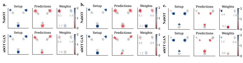
Figure 2: Unbalanced sample mapping. In all three scenarios (a,b,c), the source (gray) and target (blue) datasets share structure but have different shifts and per-cluster sampling proportions. Tasked with mapping from source to target, NubOT and ubOT GAN predict the locations (middle pane, red) and weights (right pane) of the transported samples. The number next to the weights denotes the mean weights per cluster. While both methods map the samples to the correct location, NubOT more accurately predicts the weights needed to match the target distribution, creating mass (dark blue) or destroying it (red) as needed.

Results.

The results (setup, predicted Monge maps and weights) are displayed in Fig. 2. Both NubOT and ubOT GAN correctly map the points to the corresponding target clusters without transporting mass across clusters. NubOT also accurately models the change in cluster sizes by predicting the correct weights for each point. In contrast, ubOT GAN only captures the general trend of cluster growth and shrinkage, but does not learn the exact weights required to re-weight the cluster proportions appropriately. The exact setup and calculation of weights can be found in the §B (see Table 1).

4.2 Single-cell Perturbation Responses

Through the measurement of genomic, transcriptomic, proteomic or phenotypic profiles of cells, and the identification of different cell types and cellular states based on such measurements, biologists have revealed perturbation responses and response mechanism which would have remained obscured in bulk analysis approaches (Green & Pelkmans, 2016; Liberali et al., 2014; Kramer et al., 2022). However, single-cell measurements typically require the destruction the cells in the course of recording.

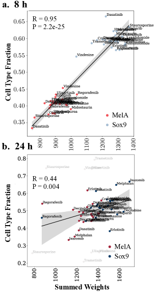
Figure 3: Given the ground truth on the known subpopulation (MelA (red) and Sox9 (blue)) sizes for each drug, we analyze their level of correlation to our predicted weights after a. 8h and b. 24h. With increasing difficulty of the task and certain drugs completely removing both or one of the subpopulations, the level of correlation reduces from 8 to 24h.

Thus, each measurement provides us only with a snapshot of cell populations, i.e., samples of probability distribution that is evolving in the course of the perturbation, from control $\mu$ (source) to perturbed cell states $\nu$ (target). Using NubOT and the considered baselines, we learn a map $T$ that reconstructs how individual cells respond to a treatment. The effect of a single perturbation frequently varies depending on the cell type or cell state, and may include the induction of cell death or proliferation. In the following, we will evaluate if NubOT is able to capture and predict heterogeneous proliferation and cell death rates of two co-cultures melanoma cell liens through $\eta$ and $\zeta$ in response to 25 drug treatments.

Figure 4: Distributional fit of the predicted perturbed cell states to the observed perturbed cell states for each drug and timestep, measured by a weighted version of kernel MMD on a set of held-out control cells. For NubOT and ubOT GAN, MMD is weighted by the predicted weights, while for the other baselines it is computed with uniform weights. Observed corresponds to a random permutation of the observed control cells, i.e., its distribution is approximately the same as the observed cells.

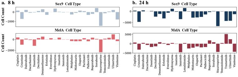
Figure 11: Drug treatment-induced change in cell counts in the two cell types compared to the cell count of the respective cell types in the control condition. a. Cell count change for cell types Sox9⁺ (top) and MelA⁺ (bottom) at $t=8h$. b. Cell count change for cell types Sox9⁺ (top) and MelA⁺ (bottom) at $t=24h$.

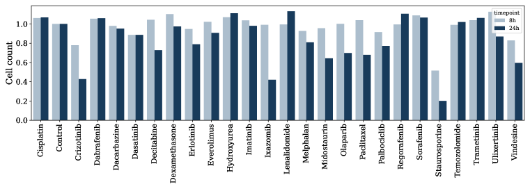
Figure 13: Observed cell counts of drug-treated cells normalized to control cell counts, per drug and time point. 8h treatment in light blue, 24h treatment in dark blue.

The single-cell measurements used for this task were generated using the imaging technology 4i (Gut et al., 2018) over the course of 24 hours, resulting in three different unaligned snapshots ($t=0h$, $t=8h$ and $t=24h$) for each of the drug treatments. The control cells, i.e., the source distribution $\mu$, consists of cells taken from a mixture of melanoma cell lines at $t=0h$ that are exposed to a dimethyl sulfoxide (DMSO) as a vehicle control. Futher, We consider two different target populations $\nu$ capturing the perturbed populations after $t=8h$ and $t=24h$ of treatment, respectively. As both cancer cell lines exhibit different sensitivities to the drugs (Raaijmakers et al., 2015), their proportion (Fig. 11) as well as the total cell counts (Fig. 13) vary over the time points. Both cell lines are characterized by the expression of mutually exclusive protein markers, i.e., one cell line strongly expresses a set of proteins detected by an antibody called MelA (MelA⁺ cell type), while the other is characterized by high levels of the protein Sox9 (Sox9⁺ cell type). An evaluation of this cell line annotation can be found in Fig. 10 (8h) and Fig. 12 (24h). Contrary to the synthetic task in § 4.2, the nature of these measurements destroys the ground truth matching. We thus use insights from the number of cells after 8 and 24 hours of treatment (Fig. 11, 13), as well as the cell type annotation for each cell to further evaluate NubOT’s performance. A detailed description of the dataset can be found in § C.2.

Results.

We split the dataset into a train and test set and train NubOT as well as the baselines on unaligned unperturbed (control) and perturbed cell populations for each drug. During evaluation, we then predict out-of-sample the perturbed cell state from held-out control cells. Details on the network architecture and hyperparameters can be found in § D.3. NubOT and ubOT GAN additionally predict the weight associated with the perturbed predicted cells, giving insights into which cells have proliferated or died in response to the drug treatments. First, we compare how well each method fits the observed perturbed cells on the level of the entire distribution. For this, we measure the weighted version of kernel maximum mean discrepancy (MMD) between predictions and observations. More details on the evaluation metrics can be found in § D.1. The results are displayed in Fig. 4. NubOT outperforms all baselines in almost all drug perturbations, showing its effectiveness in predicting OT maps and local variation in mass.

In the absence of a ground truth and in particular, given our inability to measure (i.e., observe) cells which have died upon treatment, we are required to base further analysis of NubOT’s predictions on changes in cell count for each subpopulation (MelA⁺, Sox9⁺). Fig. 11 clearly shows that drug treatments lead to substantially different cell numbers for each of the subpopulations compared to control. For example, Ulixertinib leads to the proliferation of both subpopulations after 8h, but to pronounced cell death in Sox9⁺ and strong proliferation in MelA⁺ cells after 24h. We thus expect, that weights predicted by NubOT for all drugs correlate with the change in cell counts for each cell type (here measured as population fractions). This is indeed the case, Fig. 3 shows a high correlation between observed cell counts of the two cell types and the sum of the predicted weights of the respective cell types after 8h of treatment for all drugs. After 24 hours, treatment-induced cell death (in at least one cell type) by some drugs can be so severe at that the number of observed perturbed cells becomes too low for accurate predictions and the evaluation of the task (Fig. 13). Further, we find that drugs influence the abundance of the cell lines markers MelA and Sox9, complicating cell type classification (see Fig. 10, 12, as well as Fig. 10, 12). We ignore drugs falling into these categories and find that whilst the correlation between predicted weights and observed cell counts is reduced after 24h (see Fig. 3a), NubOT still captures the overall trend.

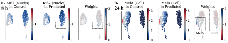
Figure 5: UMAP projections of the control cells for Ulixertinib at a. 8h and b. 24h. Cells are colored by the observed and predicted protein marker values (Ki67, MelA), and predicted weights. NubOT thereby correctly predicts weights $\geq 1$ for proliferating cells in the MelA⁺ population (a. and a., right panel), and increased levels of cell death in the Sox9⁺ population after 24h via weights $\leq 1$ (b., right panel), confirmed by the experimental observations (see Fig. 11).

The data further provides insights into biological processes such as apoptosis, a form of programmed cell death induced by enzymes called Caspases (ClCasp3). While dead cells become invisible in the cell state space (they cannot be measured), dying cells are still present in the observed perturbed sample and can be recognized by high levels of ClCasp3 (the apopotosis markers). Conversely, the protein Ki67 marks proliferating cells. Analyzing the correlation of ClCasp3 and Ki67 intensity with the predicted weights provides an additional assessment of the biological meaningfulness of our results. For example, upon Ulixertinib treatment, the absolute cell counts show an increase in Sox9⁺ cells, and a decline of MelA⁺ cells at 24h (Fig. 11). Fig. 5 shows UMAP projections of the control cells at both time points, colored by the observed and predicted protein marker values and the predicted weights. At 8h, NubOT predicts only little change in mass, but a few proliferative cells with high weights in areas which are marked by high values of the proliferation marker Ki67. At 24h, our model predicts cell death in the Sox9⁺ (MelA^-) cell type, and proliferation in the MelA⁺ cell type, which matches the observed changes in cell counts per cell type, seen in Fig. 11 in § B. We identify similar results for Trametinib (Fig. 7), Ixazomib (Fig. 8), and Vindesine (Fig. 9) which can be found in § B. These experiments thus demonstrate that NubOT accurately predicts heterogeneous drug responses at the single-cell level, capturing both, cell proliferation and death.

5 Conclusion

This work presents a novel formulation of the unbalanced optimal transport problem that bridges two previously disjoint perspectives on the topic: a theoretical one based on semi-couplings and a practical one based on recent neural estimation of OT maps. The resulting algorithm, NubOT, is scalable, efficient, and robust. Yet, it is effective at modeling processes that involve population growth or death, as demonstrated through various experimental results on both synthetic and real data. On the challenging single-cell perturbation task, NubOT is able to successfully predict perturbed cell states, while explicitly modeling death and proliferation. This is an unprecedented achievement in the field of single-cell biology, which currently relies on the use of markers to approximate the survival state of cell population upon drug treatment. Explicitly modeling proliferation and death at the single-cell level as part of the drug response, allows to link cellular properties observed prior to drug treatment to therapy outcomes. Thus, the application of NubOT in the fields of drug discovery and personalized medicine could be of great implications, as it allows to identify cellular properties predictive of drug efficacy.

Appendix

Appendix A Background

In the following, we provide further information and review related literature on concepts discussed throughout this work.

A.1 Unbalanced Optimal Transport

Unbalanced optimal transport is a generalization of the classical OT formulation (1), and as such allows mass to be created and destroyed throughout the transport. This relaxation has found recent use cases in various domains ranging from biology (Schiebinger et al., 2019; Yang & Uhler, 2019), imaging (Lee et al., 2019), shape registration (Bonneel & Coeurjolly, 2019), domain adaption (Fatras et al., 2021), positive-unlabeled learning (Chapel et al., 2020), to general machine learning (Janati et al., 2020; Frogner et al., 2015). Problem (6) provides a general framework of the unbalanced optimal transport problem, which can recover related notions introduced in the literature: Choosing for ${\mathcal{D}}_{f}$ the Kullback-Leibler divergence, one recovers the so-called squared Hellinger distance. Alternatively, with ${\mathcal{D}}_{f}=\ell_{2}$ norm, we arrive at Benamou (2003), while an $\ell_{1}$ norm retrieves a concept often referred to as partial OT (Figalli, 2010). The latter comprises approaches which do not rely on a relaxation of the marginal constraints as in (6). In particular, some strategies of partial OT expand the original problem by adding virtual mass to the marginals (Pele & Werman, 2009; Caffarelli & McCann, 2010; Gramfort et al., 2015), or by extending the OT map by dummy rows and columns (Sarlin et al., 2020) onto which excess mass can be transported. A further review is provided in (Peyré & Cuturi, 2019, Chapter 10.2). Recent work has furthermore developed alternative computational schemes (Chapel et al., 2021; Séjourné et al., 2022) as well as provided a computational complexity analysis (Pham et al., 2020) of the generalized Sinkhorn algorithm solving entropic regularized unbalanced OT (Chizat et al., 2018a). Besides Yang & Uhler (2019), these approaches do not provide parameterizations of the unbalanced problem and allow for an out-of-sample generalization which we consider in this work.

A.2 Cycle-Consistent Learning

The principle of cycle-consistency has been widely used for learning bi-directional transformations between two domains of interest. Cycle-consistency thereby assumes that both the forward and backward mapping are roughly inverses of each other. In particular, given unaligned points $x\in{\mathcal{X}}$ and $y\in{\mathcal{Y}}$, as well as maps $g:{\mathcal{X}}\mapsto{\mathcal{Y}}$ and $f:{\mathcal{Y}}\mapsto{\mathcal{X}}$, cycle-consistency reconstruction losses enforce $\|x-f(g(x))\|$ as well as $\|y-g(f(y))\|$ using some notion of distance $\|\cdot\|$, assuming that there exists such a ground truth bijection $g=f^{-1}$ and $f=g^{-1}$. The advantage of validating good matches by cycling between unpaired samples becomes evident through the numerous use cases to which cycle-consistency has been applied: Originally introduced within the field of computer vision (Kalal et al., 2010) and applied to image-to-image translation tasks (Zhu et al., 2017a), it has been quickly adapted to multi-modal problems (Zhu et al., 2017b), domain adaptation (Hoffman et al., 2018), and natural language processing (Shen et al., 2017). The original principle has been further generalized to settings requiring a many-to-one or surjective mapping between domains (Guo et al., 2021) via conditional variational autoencoders, dynamic notions of cycle-consistency (Zhang et al., 2021), or to time-varying applications (Dwibedi et al., 2019). These classical approaches enforce cycle-consistency by explicitly composing both maps and penalizing for any deviation from this bijection. In this work, we treat cycle-consistency differently. It is enforced implicitly by coupling the two distributions of interest through a sequence of reversible transformations: re-weighting, transforming, and re-weighting (Eq. (9) and Fig. 1).

Similarly to our work, Zhang et al. (2022) and Hur et al. (2021) establish a notion of cycle-consistency (reversibility) for a pair of pushforward operators to align two unpaired measures. Both methods rely on the Gromov-Monge distance (Mémoli & Needham, 2022), a divergence to compare probability distributions defined on different ambient spaces ${\mathcal{X}}$ and ${\mathcal{Y}}$—a setting not considered in this work. They proceed by defining a reversible metric through replacing the single Monge map by a pair of two Monge maps, i.e., $f:{\mathcal{X}}\mapsto{\mathcal{Y}}$ and $g:{\mathcal{Y}}\mapsto{\mathcal{X}}$, minimizing the objective

$$\mathrm{GM}(\mu,\nu):=\inf_{\begin{subarray}{c}f:{\mathcal{X}}\mapsto{\mathcal{Y}},f_{\sharp}\mu=\nu\\ g:{\mathcal{Y}}\mapsto{\mathcal{X}},g_{\sharp}\nu=\mu\end{subarray}}\Delta_{{\mathcal{X}}}^{p}(f;\mu)+\Delta_{{\mathcal{Y}}}^{p}(g;\nu)+\Delta_{{\mathcal{X}},{\mathcal{Y}}}^{p}(f,g;\mu,\nu),$$ (12)

$$\Delta_{{\mathcal{X}}}^{p}(f;\mu) =\left(\mathbb{E}\left[|c_{\mathcal{X}}(x,x^{\prime})-c_{\mathcal{Y}}(f(x),f(x^{\prime}))|^{p}\right]\right)^{\frac{1}{p}}$$

$$\Delta_{{\mathcal{Y}}}^{p}(g;\nu) =\left(\mathbb{E}\left[|c_{\mathcal{X}}(y,y^{\prime})-c_{\mathcal{Y}}(g(y),g(y^{\prime}))|^{p}\right]\right)^{\frac{1}{p}}$$

$$\Delta_{{\mathcal{X}},{\mathcal{Y}}}^{p}(f,g;\mu,\nu) =\left(\mathbb{E}\left[|c_{\mathcal{X}}(x,g(y))-c_{\mathcal{Y}}(f(x),y)|^{p}\right]\right)^{\frac{1}{p}}.$$

Problem (12) shows similarities to the classical cycle-consistency objective of Zhu et al. (2017a), where cycle-consistency is indirectly enforced through $\Delta_{{\mathcal{X}},{\mathcal{Y}}}^{p}$. Zhang et al. (2022) parameterize both Monge maps through neural networks in a similar fashion as done in (Yang & Uhler, 2019; Fan et al., 2021a). Our approach differs from Zhang et al. (2022); Hur et al. (2021) as we model the problem through a single Monge map with duals $f,g$, allowing us to map back-and-forth between measures $\mu$ and $\nu$, and using a different parametrization approach (ICNNs). More importantly, the approaches presented by Zhang et al. (2022); Hur et al. (2021) do not generalize to the unbalanced case. While Zhang et al. (2022) proposed an unbalanced version of (12) by relaxing the marginals as done in Chizat et al. (2018a), they require the unbalanced sample sizes to be known (i.e., $n$ and $m$ need to be fixed). In our application of interest, particle counts of the target population are, however, not known a priori.

A.3 Convex Neural Architectures

Input convex neural networks (Amos et al., 2017) are a class of neural networks that approximate the family of convex functions $\psi$ with parameters $\theta$, i.e., whose outputs $\psi_{\theta}(x)$ are convex w.r.t. an input $x$. This property is realized by placing certain constraints on the networks parameters $\theta$. More specifically, an ICNN is an $L$-layer feed-forward neural network, where each layer $l=\{0,...,L-1\}$ is given by

$$z_{l+1}=\sigma_{l}(W^{x}_{l}x+W^{z}_{l}z_{l}+b_{l})\text{ and }\psi_{\theta}(x)=z_{L},$$ (13)

where $\sigma_{k}$ are convex non-decreasing activation functions, and $\theta=\{W^{x}_{l},W^{z}_{l},b_{l}\}_{l=0}^{L-1}$ is the set of parameters, with all entries in $W^{z}_{l}$ being non-negative and the convention that $z_{0}$ and $W^{z}_{0}$ are $0$. As mentioned above and through the connection established in § 2, convex neural networks have been utilized to approximate Monge map $T$ (3) via the convex Brenier potential $\psi$ connected to the primal and dual optimal transport problem. In particular, it has been used to model convex dual functions (Makkuva et al., 2020) as well as normalizing flows derived from convex potentials (Huang et al., 2021). The expressivity and universal approximation properties of ICNNs have been further studied by Chen et al. (2019), who show that any convex function over a compact convex domain can be approximated in sup norm by an ICNN. To improve convergence and robustness of ICNNs —known to be notoriously difficult to train (Richter-Powell et al., 2021)— different initialization schemes have been proposed: Bunne et al. (2022b) derive two initialization schemes ensuring that upon initialization $\nabla\psi$ mimics an affine Monge map $T$ mapping either the source measure onto itself (identity initialization) or providing a map between Gaussian approximations of measures $\mu$ and $\nu$ (Gaussian initialization). Further, Korotin et al. (2020) proposed to use quadratic layers as well as a pre-training pipeline to initialize ICNN parameters to encode an identity map.

Appendix B Additional Experimental Results

B.1 Synthetic Data

In our synthetic two-dimensional dataset, the source and target distribution are mixtures of Gaussians with varying proportions (see Fig. 2). Both source and target consist of three corresponding clusters, and by changing the proportions of each cluster, we illustrate a scenario in which subpopulations grow and shrink at different rates. Table 1 shows the shares of the three clusters in the source and target distributions. In order to match the target distribution without transporting mass across non-corresponding clusters, the clusters have to be re-scaled with the factors presented in column ’True Scaling Factor’. The last two columns show the mean weights per cluster obtained by NubOT and ubOT GAN, respectively. ubOT GAN captures only the general trend in growth and shrinkage, the exact weights do not scale the cluster proportions appropriately. In contrast, the weights obtained by NubOT match the required scaling factors very closely. Fig. 6, shows the weighted MMD between the source distribution and the target distribution, confirming superior performance of NubOT.

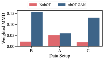
Figure 6: Distributional fit of the predicted samples to the target samples on synthetic data, measured by a weighted version of kernel MMD.

Table 1: Setup of the synthetic mixture of Gaussians dataset, showing the proportions of the three clusters in source and target distribution in three different settings (a., b., c.) as well as the required scaling factor per cluster needed to match the target without transporting points to non-corresponding clusters. The last two columns show the mean weights obtained by NubOT and ubOT GAN.

	Cluster	Source Proportions ($p$)	Target Proportions ($q$)	True Scaling Factor ($q/p$)	Mean Weight NubOT	Mean Weight ubOT GAN
a.	1	0.33	0.45	1.35	1.32	1.02
	2	0.33	0.45	1.35	1.36	0.99
	3	0.33	0.10	0.30	0.26	0.8
b.	1	0.33	0.70	2.10	2.07	1.18
	2	0.33	0.20	0.60	0.64	0.88
	3	0.33	0.10	0.30	0.29	0.81
c.	1	0.45	0.10	0.22	0.23	0.79
	2	0.45	0.45	1.00	0.98	0.94
	3	0.10	0.45	4.50	4.60	1.44

B.2 Single-Cell Perturbation Responses

As we lack ground truth for the correspondence of control and perturbed cells, we assess the biological meaningfulness of our predictions by comparing the weights to ClCasp3 and Ki67 intensity, the apoptosis and proliferation markers, respectively. Figures 7, 8 and 9 show UMAP projections computed on control cells for the drugs Trametinib, Ixazomib and Vindesine. In Figure 8 c., d., and Figure 9 c., d., regions of low predicted weights accurately correspond to regions of increased ClCasp3 intensity. Additionally, we compare predicted weights between the two cell types, and contrast them with observed cell counts.

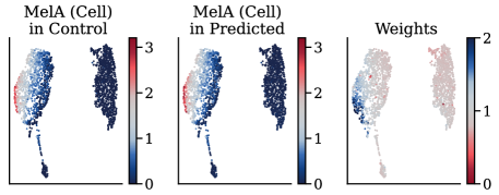
Figure 7: UMAP projections computed on control cells for Trametinib at $t=24h$. High predicted weights in the MelA⁺ cell type suggest proliferation, while the Sox9⁺ population shows higher levels of cell death. This prediction is confirmed by the relative cell counts, where MelA⁺ cell counts increase and Sox9⁺ counts decrease, demonstrating opposite response behaviors to Trametinib for each subpopulation, i.e., MelA⁺ cells show proliferation and Sox9⁺ cells death.

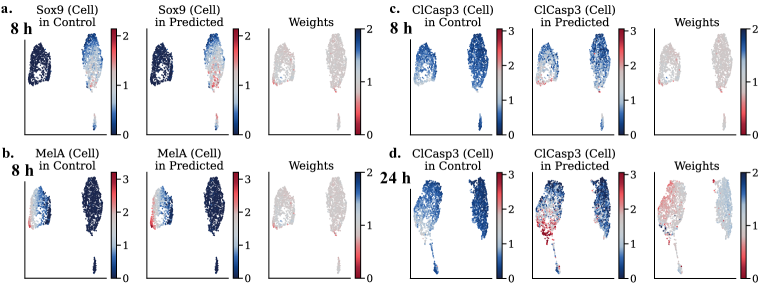
Figure 8: UMAP projections computed on control cells for Ixazomib for $t=8h$, and $t=24h$, colored by protein marker intensities a. MelA and b. Sox9, markers for the two subpopulations, as well as ClCasp3, a marker for cell death, at c. 8h and d. 24h. The UMAPs confirm the measured relative cell counts of each subpopulation. After 8h a.-c., neither MelA⁺ nor Sox9⁺ cells are affected by the treatment, i.e., we mainly predict weights around 1. d. After 24h, we observe low weights in regions of high predicted apoptosis marker intensities (ClCasp3), especially at $t=24h$, where the observed cell counts suggest death predominantly in the MelA⁺ cell cluster.

Figure 9: UMAP projections computed on control cells for Vindesine for $t=8h$, and $t=24h$, colored by protein marker intensities a. MelA and b. Sox9, markers for the two subpopulations, as well as ClCasp3, a marker for cell death, at c. 8h and d. 24h. The predicted weights (left) at c. 8h and d. 24h match the observed effects on each subpopulation, as initially only Sox9⁺ cells are affected by treatment with Vindesine, and only after 24h MelA⁺ cells show increased cell death.

Appendix C Datasets

We evaluate NubOT on several tasks including synthetic data as well as perturbation responses of single cells. In both settings, we are provided with unpaired measures $\mu$ and $\nu$ and aim to recover map $T$ which describes how source $\mu$ transforms into target $\nu$. While in the synthetic data setting we are provided with a ground truth matching, this is not the case for the single-cell data as measuring a cell requires destroying it. In the following, we describe generation and characteristics of both datasets, as well as introduce additional biological insights allowing us to shed light on the learned matching $T$.

C.1 Synthetic Data

To evaluate NubOT in a simple and low-dimensional setup with known ground-truth, we generate synthetic example: We model a source population with clear subpopulation structure through a mixture of Gaussians. Next, we generate a second (target) population aligned to the source population. We then simulate an intervention to which the subpopulations respond differently, including different levels of growth and death. Specifically, we generate batches of 400 samples with three clusters with different proportions before and after the intervention. Table 1 shows the proportions of the three clusters in the source and target distribution, as well as the required weight-factor and the obtained results from NubOT and ubOT GAN.

C.2 Single-Cell Data

Biological experiment.

The single-cell dataset used in this work was generated by the a multiplexed microscopy technology called Iterative Indirect Immunofluorescence Imaging (4i) (Gut et al., 2018), which is capable of measuring the abundance and localization of many proteins in cells. By iteratively adding, imaging and removing fluorescently tagged antibodies, a multitude of protein markers is captured for each cell. Additionally, cellular and morphological characteristics are extracted from microscopical images, such as the cell and nucleus area and circularity. This spatially resolved phenotypic dataset is rich in molecular information and provides insights into heterogeneous responses of thousands of cells to various drugs. Measuring different morphological and signaling features captures pre-existing cell-to-cell variability which might influence perturbation effect, resulting in various different responses. Some of these markers are of particular importance, as they provide insights into the level of a cell’s growth or death as well as subpopulation identity. We utilized a mixture of two melanoma tumor cell lines (M130219 and M130429) at a ratio of 1:1. The cell lines can be differentiated by the mutually exclusive expression of marker proteins. The former is positive for Sox9, the latter for a set of four proteins which are all recognized by and antibody called MelA (Raaijmakers et al., 2015). Cells were seeded in a 384-well plate and incubated at 37C and 5% CO2 overnight. Next, the cells were exposed to multiple cancer drugs and Dimethyl sulfoxide (DMSO) as a vehicle control for 8h and 24h after which the cells were fixed and six cycles of 4i were performed TissueMAPS and the scikit-image library (Van der Walt et al., 2014) were used to process and analyze the acquired images, perform feature extraction and quality control steps using semi-supervised random forest classifiers.

Data generation and processing.

Our datasets contain high-dimensional single-cell data of control and drug-treated cells measured at two time points (8 and 24 hours). For both the 8h-dataset and the 24h-dataset, we normalized the extracted intensity and morphological features by dividing each feature by its 75th percentile, computed on the control cells. Additionally, values were transformed by a $log1p$ function ($x\leftarrow log(x+1)$). In total, our datasets consist of 48 features, of which 26 are protein marker intensities and the remaining 22 are morphological features. For each treatment, we have measured between 2000 and 3000 cells. For training the models, we perform a 80/20 train/test split. We trained all models on control and treated cells for each time step and each drug separately. The considered drugs as well as their inhibition type can be found in Table 2.

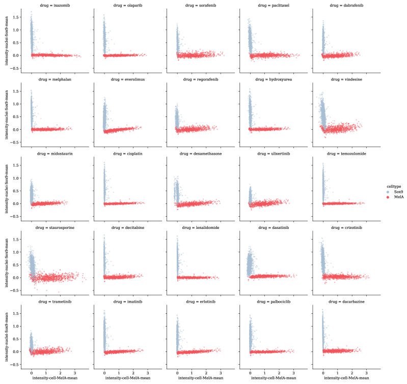
Figure 10: Classification of cells into cell types (MelA⁺, Sox9⁺) based on protein marker intensities of MelA and Sox9, for all drugs, at $t=8h$ § C.2. Each tile represents one drug. MelA⁺ cells colored in red, Sox9⁺ in blue.

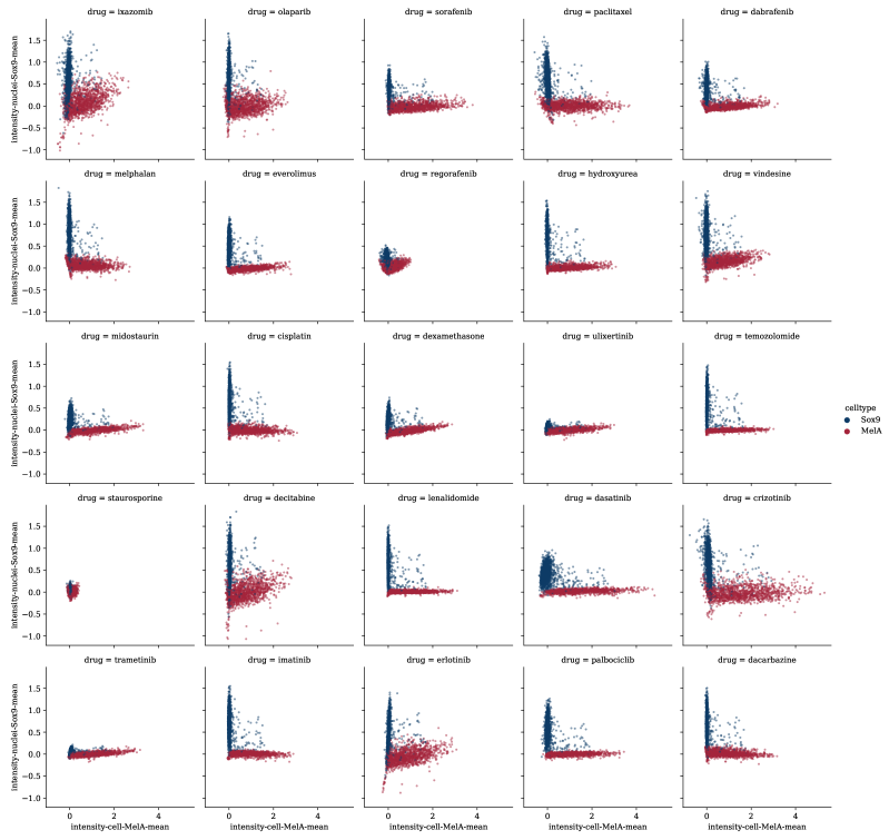
Figure 12: Classification of cells into cell types (MelA⁺, Sox9⁺) based on protein marker intensities of MelA and SOX9, for all drugs, at $t=24h$ § C.2. MelA⁺ cells colored in red, Sox9⁺ in blue.

Table 2: Overview of all treatments and their inhibition type considered in this work. Abbreviations PROTi (Proteasome inhibitor), DNASynthi (DNA synthesis inhibitor), panKi (pan kinase inhibitor), ImmuneMod. (Immune modulatory compound), MTDisruptor (Microtubule disruptor), ApopInducer (Apoptosis inducer).

Drug Name	Inhibitor Type	Drug Name	Inhibitor Type
Ixazomib	PROTi	Olaparib	PARPi
Sorafenib	RAFi	Paclitaxel	MTDisruptor
Dabrafenib	BRAFi	Melphalan	Alkylator
Everolimus	mTORi	Regorafenib	panKi
Hydroxyurea	DNASynti	Vindesine	MTDisruptor
Midostaurin	panKi	Cisplatin	Alkalyting
Dexamethasone	ImmuneMod.	Ulixertinib	ERKi
Temozolomide	Alkylator	Staurosporine	ApopInducer
Decitabine	DNAMeti	Lenalidomide	ImmuneMod.
Dasatinib	SRCi-ABLi	Crizotinib	METi
Trametinib	MEKi	Imatinib	KITi-PDGFRi-ABLi
Erlotinib	EGFRi	Palbociclib	CDK4/6i
Dacarbazine	Alkylator

Cell type assignment.

We assigned M130219 and M130429 cells to the Sox9 and MelA cell types, respectively, by first training a two component Gaussian mixture model on the features ’intensity-cell-MelA-mean’ and ’intensity-nuclei-Sox9-mean’ of the control cells. Next, we used the aforementioned features and the labels provided by the mixture model to train a nearest neighbor classifier, which we then used to predict the cell type labels of the drug treated cells. The procedure was performed separately for the 8h- and 24h dataset. Results of the classification can be found in Figure 10 and Figure 12 respectively.

Appendix D Experimental Details

NubOT consists of several modules and its performance is compared against several baselines. In the following, we provide additional background on experimental details, including a description of the evaluation metrics and baselines considered, as well as further information on the parameterization and hyperparameter choices made for NubOT.

D.1 Evaluation Metrics

We evaluate our model by analyzing the distributional similarity between the predicted and observed perturbed distribution. For this, we compute the kernel maximum mean discrepancy (MMD) (Gretton et al., 2012). To take the mass variation into consideration, we compute a weighted version of MMD, by weighting each predicted point by its associated normalized weight.

D.2 Baselines

We compare NubOT against several baselines, comprising a balanced OT-based method (Bunne et al., 2021, CellOT) and an unbalanced OT-based method (Yang & Uhler, 2019, NubOT), i.e., current state-of-the-art methods as well as ablations of our work. In the following, we briefly motivate and introduce each baseline.

CellOT.

By introducing reweighting functions $\eta$ and $\zeta$, NubOT recovers a balanced problem parameterized by dual potentials $f$ and $g$. An important ablation study to consider is thus to compare its performance to its balanced counterpart. Ignoring the fact that the original problem includes cell death and growth, and thus varying cell numbers, we apply ideas developed in Makkuva et al. (2020); Bunne et al. (2021) and learn a balanced OT problem via duals $f$ and $g$. These duals are parameterized by two ICNNs and optimized in objective (5) via an alternating min-max scheme.

ubOT GAN.

Using (6), Yang & Uhler (2019) propose to model mass variation in unbalanced OT via a relaxation of the marginals. Similar to Fan et al. (2021a), Yang & Uhler (2019) reformulate the constrained Monge problem (3) as a saddle point problem with Lagrange multiplier $h$ for the constraint $T_{\sharp}\mu=\nu$, i.e.,

$$\sup_{h}\inf_{T} \int_{{\mathcal{X}}}c(x,T(x))\mu(x)dx+\int_{{\mathcal{X}}}h(y)\left(\nu-T_{\sharp}\mu\right)dy$$

$$= \int_{{\mathcal{X}}}[c(x,T(x))-h(T(x))]\mu(x)dx+\int_{{\mathcal{X}}}h(y)\nu(y)dy,$$

parameterizing $T$ and $h$ via neural networks. To allow mass to be created and destroyed, Yang & Uhler (2019) introduce scaling factor $\xi:\mathcal{X}\rightarrow\mathbb{R}^{+}$, allowing to scale mass of each source point $x_{i}$. The optimal solution then needs to balance the cost of mass and the cost of transport, potentially measured through different cost functions $c_{1}:\mathcal{X}\times\mathcal{Y}\rightarrow\mathbb{R}^{+}$ (cost of mass transport) and $c_{2}:\mathbb{R}^{+}\rightarrow\mathbb{R}^{+}$ (cost of mass variation). Parameterizing the transport map $T_{\theta}$, the scaling factors $\xi_{\phi}$, and the penalty $h_{\omega}$ with neural networks, the resulting objective is

$$l(\theta,\phi,\omega)\coloneqq\frac{1}{n}\sum_{i=0}^{n}\left[c_{1}(x_{i},T_{\theta}(x_{i}))\xi_{\phi}(x_{i})+c_{2}(\xi_{\phi}(x_{i}))+\xi_{\phi}(x_{i})h_{\omega}(T_{\theta}(x_{i})-\Psi^{*}(h_{\omega}(y_{i})\right],$$

with $\Psi^{*}$ approximating the divergence term of the relaxed marginal constraints (see (6)), and is optimized via alternating gradient updates.

Identity.

A trivial baseline is to compare the predictions to a map which does not model any perturbation effect. The Identity baseline thus models an identity map and provides an upper bound on the overall performance, also considered in Bunne et al. (2021).

Observed.

In a similar fashion we might ask for a lower bound on the performance. As a ground truth matching is not available, we can construct a baseline for a comparison on a distributional level by comprising a different set of observed perturbed cells, which only vary from the true predictions up to experimental noise. The closer a method can approach the Observed baseline, the more accurate it fits the perturbed cell population.

D.3 Hyperparameters

We parameterize the duals $f$ and $g$ using ICNNs with 4 hidden layers, each of size 64, using ReLU as activation function between the layers. We choose the identity initialization scheme introduced by Bunne et al. (2022b) such that $\nabla g$ and $\nabla f$ resemble the identity function in the first training iteration. As suggested by Makkuva et al. (2020), we relax the convexity constraint on ICNN $g$ and instead penalize its negative weights $W^{z}_{l}$

$$R\left(\theta\right)=\lambda\sum_{W^{z}_{l}\in\theta}\left\|\max\left(-W^{z}_{l},0\right)\right\|_{F}^{2}.$$

The convexity constraint on ICNN $f$ is enforced after each update by setting the negative weights of all $W^{z}_{l}\in\theta_{f}$ to zero. Duals $g$ and $f$ are trained with an alternating min-max scheme where each model is trained at the same frequency. Further, both reweighting functions $\eta$ and $\zeta$ are represented by a multi-layer perceptron (MLP) with two hidden layers of size 64 for the single-cell and of size 32 for the synthetic dataset, with ReLU activation functions. The final output is further passed through a softplus activation function as we do not assume negative weights. For the unbalanced Sinkhorn algorithm, we choose an entropy regularization of $\varepsilon=0.005$ and a marginal relaxation penalty of $0.05$. We use both Adam for pairs $g$ and $f$ as well as $\eta$ and $\zeta$ with learning rate $10^{-4}$ and $10^{-3}$ as well as $\beta_{1}=0.5$ and $\beta_{2}=0.9$, respectively. We parameterize both baselines with networks of similar size and follow the implementation proposed by Yang & Uhler (2019) and Bunne et al. (2021).

Appendix E Reproducibility

The code will be made public upon publication of this work.

References

- Alvarez-Melis et al. (2022) David Alvarez-Melis, Yair Schiff, and Youssef Mroueh. Optimizing Functionals on the Space of Probabilities with Input Convex Neural Networks. Transactions on Machine Learning Research (TMLR), 2022.
- Amos et al. (2017) Brandon Amos, Lei Xu, and J Zico Kolter. Input Convex Neural Networks. In International Conference on Machine Learning (ICML), volume 34, 2017.
- Benamou (2003) Jean-David Benamou. Numerical resolution of an “unbalanced” mass transport problem. ESAIM: Mathematical Modeling and Numerical Analysis, 37(5), 2003.
- Benamou et al. (2015) Jean-David Benamou, Guillaume Carlier, Marco Cuturi, Luca Nenna, and Gabriel Peyré. Iterative Bregman Projections for Regularized Transportation Problems. SIAM Journal on Scientific Computing, 37(2), 2015.
- Bonneel & Coeurjolly (2019) Nicolas Bonneel and David Coeurjolly. SPOT: Sliced Partial Optimal Transport. ACM Transactions on Graphics (TOG), 38(4), 2019.
- Brenier (1987) Yann Brenier. Décomposition polaire et réarrangement monotone des champs de vecteurs. CR Acad. Sci. Paris Sér. I Math., 305, 1987.
- Bunne et al. (2021) Charlotte Bunne, Stefan G Stark, Gabriele Gut, Jacobo Sarabia del Castillo, Kjong-Van Lehmann, Lucas Pelkmans, Andreas Krause, and Gunnar Ratsch. Learning Single-Cell Perturbation Responses using Neural Optimal Transport. bioRxiv, 2021.
- Bunne et al. (2022a) Charlotte Bunne, Ya-Ping Hsieh, Marci Cuturi, and Andreas Krause. Recovering Stochastic Dynamics via Gaussian Schrödinger Bridges. arXiv Preprint arXiv:2202.05722, 2022a.
- Bunne et al. (2022b) Charlotte Bunne, Andreas Krause, and Marco Cuturi. Supervised Training of Conditional Monge Maps. In Advances in Neural Information Processing Systems (NeurIPS), volume 36, 2022b.
- Bunne et al. (2022c) Charlotte Bunne, Laetitia Meng-Papaxanthos, Andreas Krause, and Marco Cuturi. Proximal Optimal Transport Modeling of Population Dynamics. In International Conference on Artificial Intelligence and Statistics (AISTATS), volume 25, 2022c.
- Caffarelli & McCann (2010) Luis A Caffarelli and Robert J McCann. Free boundaries in optimal transport and Monge-Àmpere obstacle problems. Annals of Mathematics, 2010.
- Chapel et al. (2020) Laetitia Chapel, Mokhtar Z Alaya, and Gilles Gasso. Partial Optimal Transport with Applications on Positive-Unlabeled Learning. In Advances in Neural Information Processing Systems (NeurIPS), volume 33, 2020.
- Chapel et al. (2021) Laetitia Chapel, Rémi Flamary, Haoran Wu, Cédric Févotte, and Gilles Gasso. Unbalanced Optimal Transport through Non-negative Penalized Linear Regression. Advances in Neural Information Processing Systems (NeurIPS), 34, 2021.
- Chen et al. (2019) Yize Chen, Yuanyuan Shi, and Baosen Zhang. Optimal Control Via Neural Networks: A Convex Approach. In International Conference on Learning Representations (ICLR), 2019.
- Chizat et al. (2018a) Lenaic Chizat, Gabriel Peyré, Bernhard Schmitzer, and François-Xavier Vialard. Scaling algorithms for unbalanced optimal transport problems. Mathematics of Computation, 87(314), 2018a.
- Chizat et al. (2018b) Lenaic Chizat, Gabriel Peyré, Bernhard Schmitzer, and François-Xavier Vialard. Unbalanced optimal transport: Dynamic and Kantorovich formulations. Journal of Functional Analysis, 274(11), 2018b.
- Cuturi (2013) Marco Cuturi. Sinkhorn Distances: Lightspeed Computation of Optimal Transport. In Advances in Neural Information Processing Systems (NeurIPS), volume 26, 2013.
- Dixit et al. (2016) Atray Dixit, Oren Parnas, Biyu Li, Jenny Chen, Charles P Fulco, Livnat Jerby-Arnon, Nemanja D Marjanovic, Danielle Dionne, Tyler Burks, Raktima Raychowdhury, et al. Perturb-Seq: Dissecting Molecular Circuits with Scalable Single-Cell RNA Profiling of Pooled Genetic Screens. Cell, 167(7), 2016.
- Dwibedi et al. (2019) Debidatta Dwibedi, Yusuf Aytar, Jonathan Tompson, Pierre Sermanet, and Andrew Zisserman. Temporal Cycle-Consistency Learning. In IEEE Conference on Computer Vision and Pattern Recognition (CVPR), 2019.
- Fan et al. (2021a) Jiaojiao Fan, Shu Liu, Shaojun Ma, Yongxin Chen, and Haomin Zhou. Scalable Computation of Monge Maps with General Costs. arXiv preprint arXiv:2106.03812, 2021a.
- Fan et al. (2021b) Jiaojiao Fan, Amirhossein Taghvaei, and Yongxin Chen. Scalable Computations of Wasserstein Barycenter via Input Convex Neural Networks. In International Conference on Machine Learning (ICML), 2021b.
- Fatras et al. (2021) Kilian Fatras, Thibault Séjourné, Rémi Flamary, and Nicolas Courty. Unbalanced minibatch Optimal Transport; applications to Domain Adaptation. In International Conference on Machine Learning (ICML), 2021.
- Figalli (2010) Alessio Figalli. The Optimal Partial Transport Problem. Archive for Rational Mechanics and Analysis, 195(2), 2010.
- Frogner et al. (2015) Charlie Frogner, Chiyuan Zhang, Hossein Mobahi, Mauricio Araya, and Tomaso A Poggio. Learning with a Wasserstein loss. In Advances in Neural Information Processing Systems (NeurIPS), volume 28, 2015.
- Gramfort et al. (2015) Alexandre Gramfort, Gabriel Peyré, and Marco Cuturi. Fast Optimal Transport Averaging of Neuroimaging Data. In International Conference on Information Processing in Medical Imaging (IPMI). Springer, 2015.
- Green & Pelkmans (2016) Victoria A Green and Lucas Pelkmans. A systems survey of progressive host-cell reorganization during rotavirus infection. Cell Host & Microbe, 20(1), 2016.
- Gretton et al. (2012) Arthur Gretton, Karsten M Borgwardt, Malte J Rasch, Bernhard Schölkopf, and Alexander Smola. A kernel two-sample test. Journal of Machine Learning Research, 13, 2012.
- Guo et al. (2021) Qipeng Guo, Zhijing Jin, Ziyu Wang, Xipeng Qiu, Weinan Zhang, Jun Zhu, Zheng Zhang, and Wipf David. Fork or Fail: Cycle-Consistent Training with Many-to-One Mappings. In International Conference on Artificial Intelligence and Statistics (AISTATS), 2021.
- Gut et al. (2018) Gabriele Gut, Markus D. Herrmann, and Lucas Pelkmans. Multiplexed protein maps link subcellular organization to cellular states. Science, 361(6401), 2018.
- Hellinger (1909) Ernst Hellinger. Neue Begründung der Theorie quadratischer Formen von unendlichvielen Veränderlichen. Journal für die reine und angewandte Mathematik, 1909(136), 1909.
- Hoffman et al. (2018) Judy Hoffman, Eric Tzeng, Taesung Park, Jun-Yan Zhu, Phillip Isola, Kate Saenko, Alexei Efros, and Trevor Darrell. CyCADA: Cycle-Consistent Adversarial Domain Adaptation. In International Conference on Machine Learning (ICML), 2018.
- Huang et al. (2021) Chin-Wei Huang, Ricky T. Q. Chen, Christos Tsirigotis, and Aaron Courville. Convex Potential Flows: Universal Probability Distributions with Optimal Transport and Convex Optimization. In International Conference on Learning Representations (ICLR), 2021.
- Hur et al. (2021) YoonHaeng Hur, Wenxuan Guo, and Tengyuan Liang. Reversible Gromov-Monge Sampler for Simulation-Based Inference. arXiv preprint arXiv:2109.14090, 2021.
- Janati et al. (2020) Hicham Janati, Marco Cuturi, and Alexandre Gramfort. Spatio-Temporal Alignments: Optimal transport through space and time. In International Conference on Artificial Intelligence and Statistics (AISTATS), volume 23, 2020.
- Kalal et al. (2010) Zdenek Kalal, Krystian Mikolajczyk, and Jiri Matas. Forward-Backward Error: Automatic Detection of Tracking Failures. In IEEE Conference on Computer Vision and Pattern Recognition (CVPR). IEEE, 2010.
- Kantorovich (1942) L Kantorovich. On the transfer of masses (in Russian). In Doklady Akademii Nauk, volume 37, 1942.
- Korotin et al. (2020) Alexander Korotin, Vage Egiazarian, Arip Asadulaev, Alexander Safin, and Evgeny Burnaev. Wasserstein-2 generative networks. In International Conference on Learning Representations, 2020.
- Korotin et al. (2021) Alexander Korotin, Lingxiao Li, Aude Genevay, Justin M Solomon, Alexander Filippov, and Evgeny Burnaev. Do neural optimal transport solvers work? a continuous wasserstein-2 benchmark. Advances in Neural Information Processing Systems, 34, 2021.
- Kramer et al. (2022) Bernhard A Kramer, Jacobo Sarabia del Castillo, and Lucas Pelkmans. Multimodal perception links cellular state to decision-making in single cells. Science, 377(6606):642–648, 2022.
- Lee et al. (2019) John Lee, Nicholas P Bertrand, and Christopher J Rozell. Parallel Unbalanced Optimal Transport Regularization for Large Scale Imaging Problems. arXiv preprint arXiv:1909.00149, 2019.
- Liberali et al. (2014) Prisca Liberali, Berend Snijder, and Lucas Pelkmans. A hierarchical map of regulatory genetic interactions in membrane trafficking. Cell, 157(6):1473–1487, 2014.
- Liero et al. (2018) Matthias Liero, Alexander Mielke, and Giuseppe Savaré. Optimal Entropy-Transport problems and a new Hellinger–Kantorovich distance between positive measures. Inventiones Mathematicae, 211(3), 2018.
- Lotfollahi et al. (2019) Mohammad Lotfollahi, F Alexander Wolf, and Fabian J Theis. scGen predicts single-cell perturbation responses. Nature Methods, 16(8), 2019.
- Makkuva et al. (2020) Ashok Makkuva, Amirhossein Taghvaei, Sewoong Oh, and Jason Lee. Optimal transport mapping via input convex neural networks. In International Conference on Machine Learning (ICML), volume 37, 2020.
- Mémoli & Needham (2022) Facundo Mémoli and Tom Needham. Distance distributions and inverse problems for metric measure spaces. Studies in Applied Mathematics, 2022.
- Monge (1781) Gaspard Monge. Mémoire sur la théorie des déblais et des remblais. Histoire de l’Académie Royale des Sciences, pp. 666–704, 1781.
- Pele & Werman (2009) Ofir Pele and Michael Werman. Fast and robust Earth Mover’s Distances. In International Conference on Computer Vision (ICCV). IEEE, 2009.
- Peyré & Cuturi (2019) Gabriel Peyré and Marco Cuturi. Computational Optimal Transport. Foundations and Trends in Machine Learning, 11(5-6), 2019. ISSN 1935-8245.
- Pham et al. (2020) Khiem Pham, Khang Le, Nhat Ho, Tung Pham, and Hung Bui. On Unbalanced Optimal Transport: An Analysis of Sinkhorn Algorithm. In International Conference on Machine Learning (ICML), 2020.
- Raaijmakers et al. (2015) Marieke IG Raaijmakers, Daniel S Widmer, Melanie Maudrich, Tabea Koch, Alice Langer, Anna Flace, Claudia Schnyder, Reinhard Dummer, and Mitchell P Levesque. A new live-cell biobank workflow efficiently recovers heterogeneous melanoma cells from native biopsies. Experimental Dermatology, 24(5):377–380, 2015.
- Richter-Powell et al. (2021) Jack Richter-Powell, Jonathan Lorraine, and Brandon Amos. Input convex gradient networks. arXiv preprint arXiv:2111.12187, 2021.
- Santambrogio (2015) Filippo Santambrogio. Optimal Transport for Applied Mathematicians. Birkhäuser, NY, 55(58-63):94, 2015.
- Sarlin et al. (2020) Paul-Edouard Sarlin, Daniel DeTone, Tomasz Malisiewicz, and Andrew Rabinovich. SuperGlue: Learning Feature Matching with Graph Neural Networks. In IEEE Conference on Computer Vision and Pattern Recognition (CVPR), 2020.
- Schiebinger et al. (2019) Geoffrey Schiebinger, Jian Shu, Marcin Tabaka, Brian Cleary, Vidya Subramanian, Aryeh Solomon, Joshua Gould, Siyan Liu, Stacie Lin, Peter Berube, et al. Optimal-Transport Analysis of Single-Cell Gene Expression Identifies Developmental Trajectories in Reprogramming. Cell, 176(4), 2019.
- Séjourné et al. (2022) Thibault Séjourné, François-Xavier Vialard, and Gabriel Peyré. Faster Unbalanced Optimal Transport: Translation invariant Sinkhorn and 1-D Frank-Wolfe. In International Conference on Artificial Intelligence and Statistics (AISTATS), 2022.
- Sheldon et al. (2007) Daniel Sheldon, MA Elmohamed, and Dexter Kozen. Collective Inference on Markov Models for Modeling Bird Migration. In Advances in Neural Information Processing Systems (NeurIPS), volume 20, 2007.
- Shen et al. (2017) Tianxiao Shen, Tao Lei, Regina Barzilay, and Tommi Jaakkola. Style Transfer from Non-Parallel Text by Cross-Alignment. Advances in Neural Information Processing Systems (NeurIPS), 30, 2017.
- Tong et al. (2020) Alexander Tong, Jessie Huang, Guy Wolf, David Van Dijk, and Smita Krishnaswamy. TrajectoryNet: A Dynamic Optimal Transport Network for Modeling Cellular Dynamics. In International Conference on Machine Learning (ICML), 2020.
- Van der Walt et al. (2014) Stefan Van der Walt, Johannes L Schönberger, Juan Nunez-Iglesias, François Boulogne, Joshua D Warner, Neil Yager, Emmanuelle Gouillart, and Tony Yu. scikit-image: image processing in python. PeerJ, 2:e453, 2014.
- Yang & Uhler (2019) Karren D Yang and Caroline Uhler. Scalable Unbalanced Optimal Transport using Generative Adversarial Networks. International Conference on Learning Representations (ICLR), 2019.
- Yuan et al. (2021) Bo Yuan, Ciyue Shen, Augustin Luna, Anil Korkut, Debora S Marks, John Ingraham, and Chris Sander. CellBox: interpretable machine learning for perturbation biology with application to the design of cancer combination therapy. Cell Systems, 12(2), 2021.
- Zhan et al. (2019) Tianzuo Zhan, Giulia Ambrosi, Anna Maxi Wandmacher, Benedikt Rauscher, Johannes Betge, Niklas Rindtorff, Ragna S Häussler, Isabel Hinsenkamp, Leonhard Bamberg, Bernd Hessling, et al. MEK inhibitors activate Wnt signalling and induce stem cell plasticity in colorectal cancer. Nature Communications, 10(1), 2019.
- Zhang et al. (2021) Qiang Zhang, Tete Xiao, Alexei A Efros, Lerrel Pinto, and Xiaolong Wang. Learning Cross-Domain Correspondence for Control with Dynamics Cycle-Consistency. International Conference on Learning Representations (ICLR), 2021.
- Zhang et al. (2022) Zhengxin Zhang, Youssef Mroueh, Ziv Goldfeld, and Bharath Sriperumbudur. Cycle Consistent Probability Divergences Across Different Spaces. In International Conference on Artificial Intelligence and Statistics (AISTATS), 2022.
- Zhu et al. (2017a) Jun-Yan Zhu, Taesung Park, Phillip Isola, and Alexei A Efros. Unpaired Image-to-Image Translation using Cycle-Consistent Adversarial Networks. In IEEE Conference on Computer Vision and Pattern Recognition (CVPR), 2017a.
- Zhu et al. (2017b) Jun-Yan Zhu, Richard Zhang, Deepak Pathak, Trevor Darrell, Alexei A Efros, Oliver Wang, and Eli Shechtman. Toward Multimodal Image-to-Image Translation. In 30, 2017b.