$\Phi$-DVAE: Physics-Informed Dynamical Variational Autoencoders for Unstructured Data Assimilation

Abstract

Incorporating unstructured data into physical models is a challenging problem that is emerging in data assimilation. Traditional approaches focus on well-defined observation operators whose functional forms are typically assumed to be known. This prevents these methods from achieving a consistent model-data synthesis in configurations where the mapping from data-space to model-space is unknown. To address these shortcomings, in this paper we develop a physics-informed dynamical variational autoencoder ($\Phi$-DVAE) to embed diverse data streams into time-evolving physical systems described by differential equations. Our approach combines a standard, possibly nonlinear, filter for the latent state-space model and a VAE, to assimilate the unstructured data into the latent dynamical system. Unstructured data, in our example systems, comes in the form of video data and velocity field measurements, however the methodology is suitably generic to allow for arbitrary unknown observation operators. A variational Bayesian framework is used for the joint estimation of the encoding, latent states, and unknown system parameters. To demonstrate the method, we provide case studies with the Lorenz-63 ordinary differential equation, and the advection and Korteweg-de Vries partial differential equations. Our results, with synthetic data, show that $\Phi$-DVAE provides a data efficient dynamics encoding methodology which is competitive with standard approaches. Unknown parameters are recovered with uncertainty quantification, and unseen data are accurately predicted.

[cambridge] organization=Department of Engineering, University of Cambridge, addressline=Trumpington St, city=Cambridge, postcode=CB2 1PZ, country=United Kingdom

[imperial] organization=Department of Mathematics, Imperial College London, addressline=Exhibition Rd, city=London, postcode=SW7 2AZ, country=United Kingdom

[turing] organization=The Alan Turing Institute, city=London, addressline=British Library, 96 Euston Rd, postcode=NW1 2DB, country=United Kingdom

1 Introduction

Physical models, as represented by differential equations, are ubiquitous throughout engineering and the physical sciences. These equations synthesise scientific knowledge into mathematical form. However, as a description of reality they are imperfect [1], leading to the well-known problem of model misspecification [2]. At least since Kalman [3] physical modellers have been trying to reconcile their inherently misspecified models with observations [4]. Such approaches are usually either solving the inverse problem of attempting to recover model parameters from data, and/or, the data assimilation (DA) problem of conducting state inference based on a time-evolving process.

For the inverse problem, Bayesian methods are common [5, 6]. In this, prior belief in model parameters ${\mathbf{\Lambda}}$ is updated with data ${\mathbf{y}}$ to give a posterior distribution, $p({\mathbf{\Lambda}}|{\mathbf{y}})$. This describes uncertainty with parameters given the data and modelling assumptions. DA can also proceed from a Bayesian viewpoint, where inference is cast as a nonlinear state-space model (SSM) [7, 8]. The SSM is typically the combination of a time-discretised differential equation and an observation process: uncertainty enters the model through extrusive, additive errors. For a latent state variable ${\mathbf{u}}_{n}$ representing some discretised system at time $n$, with observations ${\mathbf{y}}_{n}$, the object of interest is the filtering distribution $p({\mathbf{u}}_{n}|{\mathbf{y}}_{1:n})$, where ${\mathbf{y}}_{1:n}:=\{{\mathbf{y}}_{k}\}_{k=1}^{n}$. The joint filtering and estimation problem, which estimates $p({\mathbf{u}}_{n},{\mathbf{\Lambda}}|{\mathbf{y}}_{1:n})$ has received attention in the literature (see, e.g., Kantas et al. [9] and references therein). This has been well studied in, e.g., electrical engineering [10], geophysics [11], neuroscience [12], chemical engineering [13], biochemistry [14], and hydrology [15], to name a few.

Typically in data assimilation tasks, while parameters of an observation model may be unknown, the observation model itself is assumed known [9]. This assumption breaks down in settings where data arrives in various modalities, such as videos, images, or audio, hindering the ability to perform inference. However, in such cases often the underlying variation in the data stream is due to a latent physical process, which is typically at least partially known. We refer to this setting, where the observation operator of the physical process is unknown, as the problem of unstructured data assimilation (UDA). In this work, we develop a variational Bayes (VB) [16] methodology which jointly solves the inverse and filtering problems when this observation operator is unknown. We model this unknown mapping with a variational autoencoder (VAE) [17], which encodes the assumed time-dependent observations ${\mathbf{y}}_{1:N}$ into pseudo-data ${\mathbf{x}}_{1:N}$ in a latent space. On this latent space, we stipulate that the pseudo-observations are taken from a known dynamical system, given by a stochastic differential equation with possibly unknown coefficients. The differential equation is also assumed to have stochastic forcing, which accounts for possible model misspecification. The stipulated system gives a structured prior $p({\mathbf{x}}_{1:N}|{\mathbf{\Lambda}})$, which acts as a physics-informed regulariser whilst also enabling inference over the unknown model parameters ${\mathbf{\Lambda}}$. This prior is approximated using classical nonlinear filtering algorithms. Our framework is fully probabilistic: inference proceeds from a derived evidence lower bound (ELBO), enabling joint estimation of unknown network parameters and unknown dynamical coefficients via VB. To set the scene for this work, we now review the relevant literature.

2 Related Work

As introduced above, VAEs [17] are a popular high-dimensional encoder. A VAE defines a generative model that learns low-dimensional representations, ${\mathbf{x}}$, of high-dimensional data, ${\mathbf{y}}$, using VB in an unsupervised fashion. To perform efficient inference, a variational approximation $q_{\phi}({\mathbf{x}}|{\mathbf{y}})$ is made to the intractable posterior $p({\mathbf{x}}|{\mathbf{y}})$, via a neural network (NN). Variational parameters $\phi$ are estimated via the ELBO. Recent works have extended the VAE to high-dimensional time-series data ${\mathbf{y}}_{1:N}$, with the aim of jointly learning latent representations ${\mathbf{x}}_{1:N}$, and a dynamical system that evolves them [18]. Termed dynamical variational autoencoders (DVAEs), they enforce the dynamics with a structured prior $p({\mathbf{x}}_{1:N})$ on the latent space.

The Kalman variational autoencoder (KVAE) of [19] is a DVAE methodology, which encodes ${\mathbf{y}}_{1:N}$ into latent variables ${\mathbf{x}}_{1:N}$ that are assumed to be observations of a linear Gaussian state-space model driven by latent dynamic states ${\mathbf{u}}_{1:N}$. Assumed linear dynamics are jointly learnt with the encoder and decoder, via Kalman filtering/smoothing. Another approach is the Gaussian process (GP) VAE [20, 21, 22], which models ${\mathbf{x}}_{1:N}$ as a temporally correlated GP. The Markovian variant of [23] allows for a similar Kalman procedure as in the KVAE, except, in this instance, the dynamics are known and are given by an stochastic differential equation (SDE) approximation to the GP [24]. Yildiz et al. [25] also propose the so-called ODE²VAE, which encodes the data to an initial condition which is integrated through time using a Bayesian neural ordinary differential equation (ODE) [26]. This trajectory, only, is used to generate the reconstructions via the decoder network.

A related class of methods are deep SSM s [27, 28, 29]. These works assume that the parametric form of the SSM is unknown, and replace the transition and emission distributions with NN models, which are trained based on an ELBO. They harness the representational power of deep NNs to directly model transitions between high-dimensional states. More emphasis is placed on generative modelling and prediction than representation learning, or system identification. We also note the related works which use VAE-type architectures for video prediction tasks [30, 31, 32], and the variational recurrent approach of Chung et al. [33], which is predominantly demonstrated on speech modelling.

Methods to blend phyics and autoencoders have also been developed. A popular approach uses SINDy [34] for discovery of low-dimensional latent dynamical systems using autoencoders [35]. A predictive framework is given in Lopez and Atzberger [36], which aims to learn nonlinear dynamics by jointly optimising an ELBO. Following our notation, this learns a function which maps ${\mathbf{u}}_{n}\mapsto{\mathbf{u}}_{n+k}$, for some $k$, via a VAE. Lusch et al. [37] use a physics-informed autoencoder to linearise nonlinear dynamical systems via a Koopman approach; inference is regularised through incorporating the Koopman structure in the loss function. Otto and Rowley [38] present a similar method, and an extension of these approaches to PDE systems is given in Gin et al. [39]. Morton et al. [40] use the linear regression methods of Takeishi et al. [41] within a standard autoencoder to similarly compute the Koopman observables. Erichson et al. [42] derive an autoencoder which incorporates a linear Markovian prediction operator, similar to a Koopman operator, which uses physics-informed regulariser to promote Lyapunov stability. Hernández et al. [43] studies VAE methods to encode high-dimensional dynamical systems. Finally, we note the related work which studies the estimation of dynamical parameters within so-called “gray-box” systems, blending NN methods with known physical laws [44, 45, 46, 47]. Methods for solving Bayesian inverse problems using VAEs have been developed for stochastic differential equations [48], and notably the UQ-VAE [49] for when the forward model is known. The UQ-VAE uses observation/latent pairs for training, and the forward model used as the decoder. These methods require the observation operator to be known.

Going beyond such “gray-box” methods, deep learning methods have been increasingly applied to directly approximating partial differential equations (PDEs). Termed the physics-informed neural network (PINN) [50], physical laws corresponding to the PDE are imposed on the loss function of the NN; solutions that do not obey such laws are thus penalised. The framework is flexible, and can be used to solve high-dimensional forward problems [51, 52], or to solve inverse problems where noisy data are observed [50]. A Bayesian variant of the standard PINN has been developed in [53] to provide uncertainty quantification in the forward and inverse problem setting, using Bayesian neural networks.

Another recent advancement in solving both forward and inverse problems using deep learning is the neural operator [54]. Neural operators are parameterised maps between function spaces, and have been used to learn PDE solution operators. They are therefore discretisation-invariant models, making them robust to mesh-refinement, and able to solve super-resolution problems [55].

These model can be used in place of slower, traditional PDE solvers as efficient surrogates for the forward model, and perform comparably when used for downstream tasks such as Bayesian inversion [56]. Related variational approaches have also been developed for time-varying physical systems by parameterising time as another input to deep NNs that are used to parameterise the variational family [57, 58].

Our contribution

In this paper we propose a physics-informed dynamical variational autoencoder ($\Phi$-DVAE): a DVAE approach which imposes the additional structure of known physics on the latent space. We assume that there is a low-dimensional dynamical system generating the high-dimensional observed time-series. A NN is used to learn the unknown embedding to this lower dimensional space. On the lower-dimensional space, the embedded data are pseudo-observations of a latent dynamical system, which is, in general, derived from a numerical discretisation of a nonlinear PDE. However, the methodology is suitably generic, allowing for ODE latent systems. Inference on this latent system is done with efficient nonlinear stochastic filtering methods, enabling the use of mature DA algorithms within our framework. A probabilistically coherent VB construction allows for joint learning of both the embedding and unknown dynamical parameters.

Instead of learnt dynamics with the KVAE [19], $\Phi$-DVAE assumes a misspecified nonlinear differential equation is driving the variation in the latent space, with possibly unknown parameters. Specifying the dynamics gives a known latent transition density, which is parameterised by physics parameters instead of neural networks as in, e.g., deep SSMs [27, 28, 29]. Whilst we share commonality with latent differential equations, the $\Phi$-DVAE differs with the ODE²VAE [25] as we perform inference with this ODE/PDE, instead of learning it and leveraging it to deterministically evolve the latents. Specifying transitions via a differential equation differs the methodology to incorporating generic physics principles in the latent space [such as 37, 38, 39, 42], or generic temporal structure [such as 20, 21, 22, 23].

Our work supplements the physics-informed machine learning literature through addressing the crucial gap of embedding a physics-driven description of latent state evolution within VAEs. We also provide, to the best of our knowledge, the first contribution within this field which addresses the problem of inversion using physics-informed machine learning [seen in 48, 49, 50, 53, 55, 56] under an unknown observation operator. Results, with synthetic data, show that the method learns sensible encodings, in limited-data settings, and accurately estimates dynamical parameters, with uncertainty quantification. We further show that the method performs comparably to current approaches, and, when extrapolating beyond training data, accurately predicts future latent states.

This paper is structured as follows. The probabilistic model is described in Section 3, which shows how the known physics are embedded into the latent space of a VAE (Section 3.1). The pseudo-observation model for the physical system is defined in Section 3.2 and the pseudo-observations ${\mathbf{x}}_{1:N}$ are related to the unstructured data ${\mathbf{y}}_{1:N}$ in Section 3.3. In Section 4 we derive the variational inference in the setting of the probabilistic model. The learning objective is given by the log-marginal likelihood of the observed data ${\mathbf{y}}_{1:N}$ as defined by the probabilistic model, and we derive a tractable lower-bound approximation to this. In Sections 4.1 and 4.2 we define the inverse problem we wish to solve, and outline the algorithm for performing the inference. Experiments and results for three different examples are given in Section 5. The paper is concluded in Section 6.

3 The Probabilistic Model

In this section we define our probabilistic model; our presentation roughly follows the structure of the generative model. We first give an overview of the dependencies between variables, as described by conditional probabilities. We then cover the latent differential equation model used to describe the underlying physics. The pseudo-observation model is defined, followed by the decoder and the encoder. We assume a general SSM:

$${\mathbf{\Lambda}} \sim p({\mathbf{\Lambda}}),$$

$${\mathbf{u}}_{n}|{\mathbf{u}}_{n-1},{\mathbf{\Lambda}} \sim p({\mathbf{u}}_{n}|{\mathbf{u}}_{n-1},{\mathbf{\Lambda}}),$$

$${\mathbf{x}}_{n}|{\mathbf{u}}_{n} \sim p({\mathbf{x}}_{n}|{\mathbf{u}}_{n}),$$

$${\mathbf{y}}_{n}|{\mathbf{x}}_{n} \sim p_{\theta}({\mathbf{y}}_{n}|{\mathbf{x}}_{n}),$$

where ${\mathbf{\Lambda}}$ describes the parameters of the Markov process $\{{\mathbf{u}}_{n}\}_{n=0}^{N}$. The dynamic model $p({\mathbf{u}}_{n}|{\mathbf{u}}_{n-1},{\mathbf{\Lambda}})$ defines the evolution of this process in time. The pseudo-observation likelihood is denoted by $p({\mathbf{x}}_{n}|{\mathbf{u}}_{n})$. Parameters $\theta$ are the NN parameters for the decoder $p_{\theta}({\mathbf{y}}_{n}|{\mathbf{x}}_{n})$. The conditional independence structure imposed by the model gives

$$p({\mathbf{y}}_{1:N},{\mathbf{x}}_{1:N},{\mathbf{u}}_{1:N},{\mathbf{\Lambda}}) =p_{\theta}({\mathbf{y}}_{1:N}|{\mathbf{x}}_{1:N})p({\mathbf{x}}_{1:N}|{\mathbf{u}}_{1:N})p({\mathbf{u}}_{1:N}|{\mathbf{\Lambda}})p({\mathbf{\Lambda}}).$$ (1)

Intuitively, $\{{\mathbf{y}}_{n}\}_{n=1}^{N}$ is the sequence of high-dimensional observations, $\{{\mathbf{x}}_{n}\}_{n=1}^{N}$ is its embedding/pseudo-data, and $\{{\mathbf{u}}_{n}\}_{n=0}^{N}$ is the latent physics process. For each $n$, we assume that ${\mathbf{y}}_{n}\in{\mathbb{R}}^{n_{y}}$, ${\mathbf{x}}_{n}\in{\mathbb{R}}^{n_{x}}$, ${\mathbf{u}}_{n}\in{\mathbb{R}}^{n_{u}}$, and ${\mathbf{\Lambda}}\in{\mathbb{R}}^{n_{\lambda}}$. In what follows, we describe the components of our probabilistic model in detail.

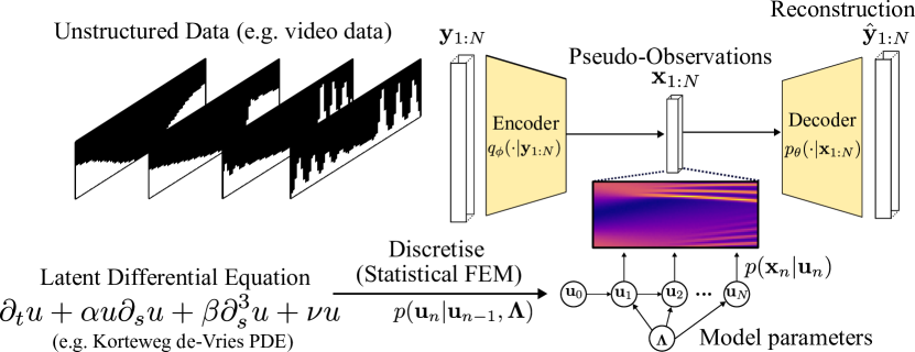
Figure 1: An illustration of the $\Phi$-DVAE model. On the left, the video frames are seen, denoted ${\mathbf{y}}_{1:N}$. These are converted into physically interpretable low-dimensional encodings ${\mathbf{x}}_{1:N}$ using an encoder. The learning is informed by the physics-driven state-space model, which treats ${\mathbf{x}}_{1:N}$ as pseudo-observations (bottom right). These pseudo-observations are used to infer the latent states ${\mathbf{u}}_{1:N}$.

3.1 Dynamic Model

The first component of the generative model is the latent dynamical system $p({\mathbf{u}}_{n}|{\mathbf{u}}_{n-1},{\mathbf{\Lambda}})$. We model this latent physics process $\{{\mathbf{u}}_{n}\}_{n=0}^{N}$ as a discretised stochastic PDE, however ODE latent physics is admissible within our framework (see Section 5.1). We discretise this process with the statistical finite element method (statFEM) [59, 60, 61, 62], forming the basis of the physics-informed prior on the latent space. Stochastic additive forcing inside the PDE represents additive model error, which results from possibly misspecified physics. Full details, including the ODE case, are given in C.

We assume that the model has possibly unknown coefficients ${\mathbf{\Lambda}}$; on these we place the Bayesian prior ${\mathbf{\Lambda}}\sim p({\mathbf{\Lambda}})$ [6], describing our a priori knowledge on the model parameters before observing any data. We also assume that ${\mathbf{u}}_{0}$, the initial condition, is known up to measurement noise, with prior $p({\mathbf{u}}_{0})$ set accordingly. For pedagogical purposes, we derive the discrete-time dynamic model using the Korteweg-de Vries (KdV) equation as a running example, which is used in later sections as an example PDE. KdV is given by:

$$\partial_{t}u+\alpha u\partial_{s}u+\beta\partial_{s}^{3}u+\nu u=\dot{\xi},\quad\dot{\xi}\sim\mathcal{GP}(0,\delta(t-t^{\prime})\cdot k(s,s^{\prime})),$$ (2)

where $u:=u(s,t)\in{\mathbb{R}}$, $\xi:=\xi(s,t)$, $s\in[0,L]$, $t\in[0,T]$, and ${\mathbf{\Lambda}}\subseteq\{\alpha,\beta,\nu\}$. Informally $\dot{\xi}$ is a GP, with delta correlations in time, and spatial correlations given by the covariance kernel $k(\cdot,\cdot)\colon{\mathbb{R}}\times{\mathbb{R}}\to{\mathbb{R}}$ [63]. This is an uncertain term in the PDE, representing possible model misspecification. Note that we assume all GP hyperparameters are known in this work. The KdV equation is used to model nonlinear internal waves [see, e.g., 64], and describes the balance between nonlinear advection and dispersion. Note that although the KdV equation defines a scalar field, $u(s,t)$, the approach similarly holds for vector fields.

Following statFEM, the equations are first spatially discretised with the finite element method (FEM) [65], then discretised in time. Equation 2 is multiplied with a smooth test function $w(s)\in W$, where $W$ is an appropriate function space, and integrated over the domain $\Omega$ to give the weak form [66]

$$\langle\partial_{t}u,w\rangle+\alpha\langle u\partial_{s}u,w\rangle+\beta\langle\partial_{s}^{3}u,w\rangle+\nu\langle u,w\rangle=\langle\dot{\xi},w\rangle,$$

where $\langle\cdot,\cdot\rangle$ is the $L^{2}(\Omega)$ inner product.

The domain is discretised to give the mesh $\Omega_{h}$ with vertices $\{s_{j}\}_{j=0}^{n_{h}}$. In this case, we take the $s_{j}$ to be a uniformly spaced set of points, so that $s_{j}=jh$ ($h$ gives the spacing between grid-points). On the mesh a set of polynomial basis functions $\{\phi_{j}(s)\}_{i=1}^{n_{u}}$ is defined, such that approximation to the PDE. Letting $u_{h}(s,t)=\sum_{i=1}^{n_{u}}u_{i}(t)\phi_{i}(s)$, the weak form is now rewritten with these basis functions

$$\langle\partial_{t}u_{h},\phi_{j}\rangle+\alpha\langle u_{h}\partial_{s}u_{h},\phi_{j}\rangle+\beta\langle\partial_{s}^{3}u_{h},\phi_{j}\rangle+\nu\langle u_{h},\phi_{j}\rangle=\langle\dot{\xi},\phi_{j}\rangle,\quad j=1,\ldots,n_{u}.$$

This gives a finite-dimensional SDE over the FEM coefficients ${\mathbf{u}}(t)=(u_{1}(t),\ldots,u_{n_{u}}(t))^{\top}$:

$${\mathbf{M}}\frac{{\mathrm{d}}{\mathbf{u}}}{{\mathrm{d}}t}+\alpha{\mathcal{F}}({\mathbf{u}})+\beta{\mathbf{A}}{\mathbf{u}}+\nu{\mathbf{M}}{\mathbf{u}}=\dot{\bm{\xi}},\quad\dot{\bm{\xi}}(t)\sim{\mathcal{N}}(\bm{0},\delta(t-t^{\prime})\cdot{\mathbf{G}}),$$

where ${\mathbf{M}}_{ij}=\langle\phi_{i},\phi_{j}\rangle$, ${\mathbf{A}}_{ji}=\langle\partial_{s}^{3}\phi_{i},\phi_{j}\rangle$, ${\mathcal{F}}({\mathbf{u}})_{j}=\langle u_{h}\partial_{s}u_{h},\phi_{j}\rangle$, and ${\mathbf{G}}_{ij}=\langle\phi_{i},\langle k(\cdot,\cdot),\phi_{j}\rangle\rangle$. Time discretisation eventually gives the transition density $p({\mathbf{u}}_{n}|{\mathbf{u}}_{n-1},{\mathbf{\Lambda}})$, for ${\mathbf{u}}_{n}={\mathbf{u}}(n\Delta_{t})$, whose form is dependent on the discretisation used (see C).

3.2 Likelihood

The second component of the generative model is the likelihood $p({\mathbf{x}}_{n}|{\mathbf{u}}_{n})$, for pseudo-data $\{{\mathbf{x}}_{n}\}_{n=1}^{N}$. The introduction of the likelihood in the model is usually necessary, as high-dimensional observations $\{{\mathbf{y}}_{n}\}_{n=1}^{N}$ may only be generated by some observed dimensions of $\{{\mathbf{u}}_{n}\}_{n=0}^{N}$. For example, perhaps it is known a priori that only a single component of a latent coupled differential equation generates the observations (see also Section 5.1). This explicit likelihood is introduced to separate the encoding process from the state-space inference; in practice we sample the pseudo-data from the variational encoding distribution ${\mathbf{x}}_{1:N}\sim q_{\phi}(\cdot|{\mathbf{y}}_{1:N})$, then condition on it with standard nonlinear filtering algorithms [19].

The latent states ${\mathbf{u}}_{n}$ are mapped at discrete times to pseudo-observations via ${\mathbf{x}}_{n}={\mathbf{H}}{\mathbf{u}}_{n}+{\mathbf{r}}_{n}$, with ${\mathbf{r}}_{n}\sim{\mathcal{N}}(\bm{0},{\mathbf{R}})$. This gives the observation density $p({\mathbf{x}}_{n}|{\mathbf{u}}_{n})={\mathcal{N}}({\mathbf{H}}{\mathbf{u}}_{n},{\mathbf{R}})$. Both the pseudo-observation operator ${\mathbf{H}}\in{\mathbb{R}}^{n_{x}\times n_{u}}$ and the noise covariance ${\mathbf{R}}\in{\mathbb{R}}^{n_{x}\times n_{x}}$ are assumed to be known in this work. The combination of the transition and observation densities provides the nonlinear Gaussian SSM:

$$\text{Transition: }\quad{\mathbf{u}}_{n} =\mathcal{M}({\mathbf{u}}_{n-1})+{\mathbf{e}}_{n-1},\quad{\mathbf{e}}_{n-1}\sim\mathcal{N}(\mathbf{0},{\mathbf{Q}}),$$

$$\text{Pseudo-observation: }\quad{\mathbf{x}}_{n} ={\mathbf{H}}{\mathbf{u}}_{n}+{\mathbf{r}}_{n},\quad{\mathbf{r}}_{n}\sim\mathcal{N}(\mathbf{0},{\mathbf{R}}).$$

Inference is performed with the extended Kalman filter (ExKF) [67, 7], which computes $p({\mathbf{u}}_{n}|{\mathbf{x}}_{1:n},{\mathbf{\Lambda}})$. Further details are contained in Section 4.

3.3 Decoder

The last component of our generative model is the decoder $p_{\theta}({\mathbf{y}}_{n}|{\mathbf{x}}_{n})$, which describes the unknown mapping between the pseudo-observations ${\mathbf{x}}_{n}$, and the observed data ${\mathbf{y}}_{n}$. The decoding of latents to data should model as closely as possible the true data generation process. Prior knowledge about this process can be used to select an appropriate $p_{\theta}({\mathbf{y}}_{n}|{\mathbf{x}}_{n})$. No temporal structure is assumed on $\theta$, so the decoder is shared across all times $p_{\theta}({\mathbf{y}}_{1:N}|{\mathbf{x}}_{1:N})=\prod_{n=1}^{N}p_{\theta}({\mathbf{y}}_{n}|{\mathbf{x}}_{n})$. For more details on specific architectures see A.

4 Variational Inference

In this section, we introduce the variational family and the ELBO. Denote by $q({\mathbf{u}}_{1:N},{\mathbf{x}}_{1:N},{\mathbf{\Lambda}}|{\mathbf{y}}_{1:N})$ the variational posterior, which, similar to Fraccaro et al. [19], factorises as

$$q({\mathbf{u}}_{1:N},{\mathbf{x}}_{1:N},{\mathbf{\Lambda}}|{\mathbf{y}}_{1:N})=q({\mathbf{u}}_{1:N}|{\mathbf{x}}_{1:N},{\mathbf{\Lambda}})q_{\phi}({\mathbf{x}}_{1:N}|{\mathbf{y}}_{1:N})q_{\lambda}({\mathbf{\Lambda}}).$$ (3)

Note here that we do not make a variational approximation $q({\mathbf{u}}_{1:N}|{\mathbf{x}}_{1:N},{\mathbf{\Lambda}})$; this is taken to be the exact posterior $p({\mathbf{u}}_{1:N}|{\mathbf{x}}_{1:N},{\mathbf{\Lambda}})$. We derive the ELBO to be (see also B)

$$\log p({\mathbf{y}}_{1:N}) \geq\int\log\left[\frac{p({\mathbf{u}}_{1:N},{\mathbf{x}}_{1:N},{\mathbf{\Lambda}},{\mathbf{y}}_{1:N})}{q({\mathbf{u}}_{1:N},{\mathbf{x}}_{1:N},{\mathbf{\Lambda}}|{\mathbf{y}}_{1:N})}\right]q({\mathbf{u}}_{1:N},{\mathbf{x}}_{1:N},{\mathbf{\Lambda}}|{\mathbf{y}}_{1:N}){\mathrm{d}}{\mathbf{x}}_{1:N}{\mathrm{d}}{\mathbf{u}}_{1:N}{\mathrm{d}}{\mathbf{\Lambda}}$$

$$=\mathbb{E}_{q_{\phi}}\left[\log\frac{p_{\theta}({\mathbf{y}}_{1:N}|{\mathbf{x}}_{1:N})}{q_{\phi}({\mathbf{x}}_{1:N}|{\mathbf{y}}_{1:N})}+\mathbb{E}_{q_{\lambda}}\left[\log p({\mathbf{x}}_{1:N}|{\mathbf{\Lambda}})+\log\frac{p({\mathbf{\Lambda}})}{q_{\lambda}({\mathbf{\Lambda}})}\right]\right].$$ (4)

Typically this expectation is not analytically tractable and Monte Carlo (MC) is used to compute an approximation. Estimating $\log p({\mathbf{x}}_{1:N}|{\mathbf{\Lambda}})$ requires marginalising over ${\mathbf{u}}_{1:N}$, the latent physics process. As detailed above, the ExKF [67, 7] recursively computes a Gaussian approximation to the filtering posterior $p({\mathbf{u}}_{n}|{\mathbf{x}}_{1:n},{\mathbf{\Lambda}})\approx{\mathcal{N}}({\mathbf{m}}_{n},{\mathbf{C}}_{n})$. We note however that this can also be realised with other nonlinear filters, e.g., ensemble Kalman filters [68] or particle filters [69]. The factorisation of the pseudo-observation marginal likelihood, $p({\mathbf{x}}_{1:N}|{\mathbf{\Lambda}})=p({\mathbf{x}}_{1}|{\mathbf{\Lambda}})\prod_{n=2}^{N}p({\mathbf{x}}_{n}|{\mathbf{x}}_{1:n-1},{\mathbf{\Lambda}})$, enables computation, as the filter can compute $p({\mathbf{x}}_{n}|{\mathbf{x}}_{1:n-1},{\mathbf{\Lambda}})$, at each prediction step, via $p({\mathbf{x}}_{n}|{\mathbf{x}}_{1:n-1},{\mathbf{\Lambda}})=\int p({\mathbf{x}}_{n}|{\mathbf{u}}_{n},{\mathbf{\Lambda}})p({\mathbf{u}}_{n}|{\mathbf{x}}_{1:n-1},{\mathbf{\Lambda}})\,{\mathrm{d}}{\mathbf{u}}_{n}$.

Encoder parameters $\phi$ are shared between variational distributions $\left\{q_{\phi}({\mathbf{x}}_{n}|{\mathbf{y}}_{n})\right\}_{n=1}^{N}$ to give an amortized approach [70]. Unless otherwise specified, for each $n$ the encoding has the form $q_{\phi}({\mathbf{x}}_{n}|{\mathbf{y}}_{n})={\mathcal{N}}(\mu_{\phi}({\mathbf{y}}_{n}),\sigma_{\phi}({\mathbf{y}}_{n}))$. Functions $\mu_{\phi}({\mathbf{y}}_{n})\colon{\mathbb{R}}^{n_{y}}\to{\mathbb{R}}^{n_{x}}$ and $\log\sigma_{\phi}({\mathbf{y}}_{n})\colon{\mathbb{R}}^{n_{y}}\to{\mathbb{R}}^{n_{x}}$ are NNs, with parameters $\phi$ to be learnt. Parameter updates are performed using the Adam optimiser [71]. Practical implementation details and specific encoding architectures are given in A. As for $q_{\lambda}$, the form of the variational approximation is set based on the parameters of interest, see Table 1 for a few candidate distributions.

4.1 Joint Learning

The inverse problem we aim to solve is the joint estimation of the filtering posterior, $p({\mathbf{u}}_{n}|{\mathbf{y}}_{1:n})$, and the dynamic parameters ${\mathbf{\Lambda}}$. Here, we assume the latent transition distribution, $p({\mathbf{u}}_{n}|{\mathbf{u}}_{n-1},{\mathbf{\Lambda}})$ is known and can be constructed from the PDE via statFEM, and treat ${\mathbf{\Lambda}}$ as a parameter we wish to estimate via the variational approximation in Eq. 3. The prior distribution $p({\mathbf{\Lambda}})$ in effect places a prior over a family of partial differential equations, whose posterior is targeted by learning the parameters of the variational approximation $q_{\lambda}({\mathbf{\Lambda}})$. These distribution parameters $\lambda$ are learned via gradient ascent of the ELBO, using MC samples from the variational posterior ${\mathbf{\Lambda}}^{(i)}\sim q_{\lambda}(\cdot)$.

Input: training data ${\mathbf{y}}_{1:N}$, SSM $\left\{\mathcal{M},{\mathbf{H}},{\mathbf{Q}},{\mathbf{R}}\right\}$, model parameter prior $p({\mathbf{\Lambda}})$, initial parameters $\left\{\phi_{0},\theta_{0},\lambda_{0}\right\}$, step number $K$

for $k=0,\dots,K-1$ do

       ${\mathbf{x}}_{1:N}\sim q_{\phi_{k}}(\cdot|{\mathbf{y}}_{1:N})$

        $\triangleright$ Sample pseudo-observations

       ${\mathbf{\Lambda}}\sim q_{\lambda_{k}}(\cdot)\;$

        $\triangleright$ Sample model parameters

       $\mathcal{L}_{k}=\log p_{\theta_{k}}({\mathbf{y}}_{1:N}|{\mathbf{x}}_{1:N})-\log q_{\phi_{k}}({\mathbf{x}}_{1:N}|{\mathbf{y}}_{1:N})+\log p({\mathbf{x}}_{1:N}|{\mathbf{\Lambda}})-\operatorname{KL}(q_{\lambda_{k}}\;\|\;p)\;$

        $\triangleright$ Calculate ELBO

       $\left(\phi_{k+1},\theta_{k+1},\lambda_{k+1}\right)=\text{Adam}\left(\nabla\mathcal{L}_{k},\phi_{k},\theta_{k},\lambda_{k}\right)\;$

        $\triangleright$ Adam update step

      

end for

return $\left(\phi_{K},\theta_{K},\lambda_{K}\right)$

Algorithm 1 $\Phi$-DVAE: joint learning of autoencoder and model parameter distribution

This relies on the KL-divergence between the prior and variational posterior being available analytically, which is the case for some choices of prior and variational posterior. We also require a closed form reparameterisation for sampling from the posterior to allow for gradient computation. Table 1 details the relevant formulae for a few popular distributions. Pseudo-code for the joint learning is provided in Algorithm 1.

Distribution	$\lambda$	Support	PDF	KL-Divergence	Reparameterise
Gaussian	$\left\{\mu,\sigma\right\}$	$x\in\mathbb{R}$	$\frac{1}{\sigma\sqrt{2\pi}}\exp\left(-\frac{(x-\mu)^{2}}{2\sigma^{2}}\right)$	$\frac{\mu_{2}}{2}-\frac{\mu_{1}}{2}-\frac{1}{2}+\frac{\sigma_{1}^{2}+(\mu_{1}-\mu_{2})^{2}}{2\sigma_{2}^{2}}$	$\mu+\sigma*Z$
Exponential	$\left\{\lambda\right\}$	$x\in\mathbb{R}^{+}$	$\lambda\exp(-\lambda x)$	$\log\left(\frac{\lambda_{1}}{\lambda_{2}}\right)+\frac{\lambda_{2}}{\lambda_{1}}-1$	$-\log(U)/\lambda$
Log-normal	$\left\{\mu,\sigma\right\}$	$x\in\mathbb{R}^{+}$	$\frac{1}{x\sigma\sqrt{2\pi}}\exp\left(-\frac{(\log(x)-\mu)^{2}}{2\sigma^{2}}\right)$	$\log\left(\frac{\sigma_{2}}{\sigma_{1}}\right)+\frac{(\mu_{1}-\mu_{2})^{2}+\sigma_{1}^{2}-\sigma_{2}^{2}}{2\sigma_{2}^{2}}$	$\exp(\mu+\sigma*Z)$

Table 1: Variational distributions for parameters, $Z\sim\mathcal{N}(0,1),U\sim\mathcal{U}[0,1]$.

4.2 Filtering Inference

Once the autoencoder parameters $\left\{\phi,\theta\right\}$ have been learned jointly with the variational parameters $\lambda$, we can assess the performance of the $\Phi$-DVAE algorithm by comparing the filtering posterior $p({\mathbf{u}}_{n}|{\mathbf{y}}_{1:n})$, to the true latent solution ${\mathbf{u}}(n\Delta_{t})$ that generated the data. This assesses the ability of both the model to provide meaningful encodings via the autoencoder, and the extended Kalman filter to give latent solutions that match the true data generating solution. This distribution can be approximated via MC samples from the variational autoencoder, marginalising over the latent encodings ${\mathbf{x}}_{1:N}$ and the model parameters ${\mathbf{\Lambda}}$. We can approximate the filtering marginal distribution at a time $n$:

$$p({\mathbf{u}}_{n}|{\mathbf{y}}_{1:n}) \approx\int p({\mathbf{u}}_{n}|{\mathbf{x}}_{1:n},{\mathbf{\Lambda}})q_{\lambda}({\mathbf{\Lambda}})q_{\phi}({\mathbf{x}}_{1:n}|{\mathbf{y}}_{1:n})\,{\mathrm{d}}{\mathbf{\Lambda}}{\mathrm{d}}{\mathbf{x}}_{1:n}$$

$$\approx\frac{1}{M}\sum_{i=1}^{M}p({\mathbf{u}}_{n}|{\mathbf{x}}_{1:n}^{(i)},{\mathbf{\Lambda}}^{(i)}),\quad{\mathbf{x}}_{1:n}^{(i)}\sim q_{\phi}(\cdot|{\mathbf{y}}_{1:n}),\;{\mathbf{\Lambda}}^{(i)}\sim q_{\lambda}(\cdot).$$ (5)

The resulting distribution is a mixture of Gaussians over the latent state, with each $p({\mathbf{u}}_{n}|{\mathbf{x}}_{1:n}^{(i)},{\mathbf{\Lambda}}^{(i)})=\mathcal{N}({\mathbf{m}}_{n}^{(i)},{\mathbf{C}}_{n}^{(i)})$.

The parameter inference can be assessed by comparing the variational posterior $q_{\lambda}({\mathbf{\Lambda}})$ to the prior distribution $p({\mathbf{\Lambda}})$ and the true coefficient value that generated the data.

Finally we can compare the performance of the joint estimation by marginalising over the parameters ${\mathbf{\Lambda}}$, and comparing this to a model that learned the autoencoder parameters conditioning only on samples from the prior $p({\mathbf{\Lambda}})$. We denote this trained prior model $\left\{\phi,\theta\right\}$, and denote the jointly trained model $\left\{\phi^{\star},\theta^{\star},\lambda^{\star}\right\}$. This should isolate the impact of learning a variational approximation to the model parameters ${\mathbf{\Lambda}}$ on the resulting latent inference and predictive power. Ideally, the learned posterior should be more concentrated around the ground truth value of the dynamic parameter, giving predictions of latent states that are closer to the true latent process. For prediction, the aim will be to infer the values of the latent process past the final time of the training dataset; these predictions are made by iterating only the prediction step of the Kalman filter ahead in time from the final mean and covariance. We will refer to these as rollout predictions, as in essence we are ‘rolling out’ the filter to provide future predictions without incorporating observations.

For the rollout, the target distribution in the latent state a number of time steps $\tau$ ahead of step $n$, i.e. $p({\mathbf{u}}_{n+\tau}|{\mathbf{y}}_{1:n})$. Consider the distribution over the latents a single time step ahead,

$$p({\mathbf{u}}_{n+1}|{\mathbf{y}}_{1:n}) \approx\int p({\mathbf{u}}_{n+1}|{\mathbf{u}}_{n},{\mathbf{\Lambda}})p({\mathbf{u}}_{n}|{\mathbf{x}}_{1:n},{\mathbf{\Lambda}})q_{\lambda}({\mathbf{\Lambda}})q_{\phi}({\mathbf{x}}_{1:n}|{\mathbf{y}}_{1:n}){\mathrm{d}}{\mathbf{u}}_{n}{\mathrm{d}}{\mathbf{x}}_{1:n}{\mathrm{d}}{\mathbf{\Lambda}}$$

$$=\int\underbrace{\left[\int p({\mathbf{u}}_{n+1}|{\mathbf{u}}_{n},{\mathbf{\Lambda}})p({\mathbf{u}}_{n}|{\mathbf{x}}_{1:n},{\mathbf{\Lambda}}){\mathrm{d}}{\mathbf{u}}_{n}\right]}_{\text{Kalman Filter Prediction Step}}q_{\lambda}({\mathbf{\Lambda}})q_{\phi}({\mathbf{x}}_{1:n}|{\mathbf{y}}_{1:n}){\mathrm{d}}{\mathbf{x}}_{1:n}{\mathrm{d}}{\mathbf{\Lambda}}$$

$$=\int p({\mathbf{u}}_{n+1}|{\mathbf{x}}_{1:n},{\mathbf{\Lambda}})q_{\lambda}({\mathbf{\Lambda}})q_{\phi}({\mathbf{x}}_{1:n}|{\mathbf{y}}_{1:n}){\mathrm{d}}{\mathbf{x}}_{1:n}{\mathrm{d}}{\mathbf{\Lambda}}$$

$$\approx\frac{1}{M}\sum_{i=1}^{M}p({\mathbf{u}}_{n+1}|{\mathbf{x}}_{1:n}^{(i)},{\mathbf{\Lambda}}^{(i)}),\quad{\mathbf{x}}_{1:n}^{(i)}\sim q_{\phi}(\cdot|{\mathbf{y}}_{1:n}),\;{\mathbf{\Lambda}}^{(i)}\sim q_{\lambda}(\cdot).$$ (6)

Here, the mixture of Gaussians distribution is constructed with the one-step-ahead predictive distributions $p({\mathbf{u}}_{n+1}|{\mathbf{x}}_{1:n}^{(i)},{\mathbf{\Lambda}}^{(i)})=\mathcal{N}(\hat{{\mathbf{m}}}_{n+1}^{(i)},\hat{{\mathbf{C}}}_{n+1}^{(i)})$. This step can be iterated on the mean and covariance to give predictions $\tau$ steps ahead, i.e. the distribution $p({\mathbf{u}}_{n+\tau}|{\mathbf{x}}_{1:n}^{(i)},{\mathbf{\Lambda}}^{(i)})$.

5 Experiments

5.1 Lorenz-63

In our first example, the latent dynamical model $p({\mathbf{u}}_{n}|{\mathbf{u}}_{n-1},{\mathbf{\Lambda}})$ is given by an Euler-Maruyama discretisation [72] of the stochastic Lorenz-63 system,

$${\mathrm{d}}{u}_{1} =(-\sigma u_{1}+\sigma u_{2}){\mathrm{d}}t+{\mathrm{d}}w_{1},$$

$${\mathrm{d}}{u}_{2} =(-u_{1}u_{3}+ru_{1}-u_{2}){\mathrm{d}}t+{\mathrm{d}}w_{2},$$ (7)

$${\mathrm{d}}{u}_{3} =(u_{1}u_{2}-bu_{3}){\mathrm{d}}t+{\mathrm{d}}w_{3},$$

where ${\mathbf{u}}(t):=[u_{1}(t),u_{2}(t),u_{3}(t)]^{\top}$, $t\in[0,6]$, ${\mathbf{u}}_{n}=[u_{1}(n\Delta_{t}),u_{2}(n\Delta_{t}),u_{3}(n\Delta_{t})]$, ${\mathbf{\Lambda}}\subseteq\left\{\sigma,r,b\right\}$, and $w_{1}$, $w_{2}$, and $w_{3}$ are independent Brownian motion processes [73].

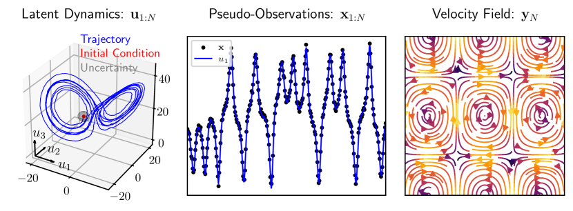
Figure 2: Lorenz-63: latent states ${\mathbf{u}}_{1:N}$, pseudo-observations ${\mathbf{x}}_{1:N}$, and velocity field ${\mathbf{y}}_{N}$.

We observe synthetic 2D velocity fields, ${\mathbf{y}}_{1:N}$ of convective fluid flow and we use our method to embed these synthetic data into the stochastic Lorenz-63 system. The Lorenz-63 system is related to the velocity fields through a truncated spectral expansion. In brief, it is assumed that the velocity fields have no vertical velocity, so the 3D velocity field is realised in 2D. The velocity field can be described by the stream function $\psi:=\psi(s_{1},s_{2},t)$, where $s_{1}$ and $s_{2}$ are the spatial coordinates of variation, respectively, and thus $\mathbf{y}(t)=\left(-\partial_{s_{2}}\psi,0,\partial_{s_{1}}\psi\right)$. A truncated spectral approximation and a transform to non-dimensional equations yields $\psi(s_{1},s_{2},t)\propto u_{1}(t)\sin(\pi s_{1}/l)\sin(\pi s_{2}/d)$, where $u_{1}(t)$ is governed by the Lorenz-63 ODE (i.e., (5.1) with $w_{i}\equiv 0$). For full details we refer to A and C. The Lorenz-63 system is classical system, popularised in Lorenz [74] through its characteristic “deterministic nonperiodic flow”: chaotic dynamics.

To generate the synthetic data ${\mathbf{y}}_{1:N}$, we generate a trajectory ${\mathbf{u}}_{1:N}^{\mathrm{true}}$ from the deterministic version of 5.1, at discrete timepoints $n\Delta_{t}$, and use the generated $u_{1,n}^{\mathrm{true}}$ to compute the two-dimensional velocity field, ${\mathbf{y}}_{n}$, via $\psi(s_{1},s_{2},t)$. This corresponds to having a middle layer $x_{n}=u_{1,n}+w_{n}$ where $w_{n}\sim\mathcal{N}(0,R^{2})$, with likelihood $p(x_{n}|{\mathbf{u}}_{n})=\mathcal{N}({\mathbf{h}}^{\top}{\mathbf{u}}_{n},R^{2})$ where ${\mathbf{h}}=[1,0,0]^{\top}$. The synthetic data of ${\mathbf{u}}^{\mathrm{true}}(t)$, ${\mathbf{x}}_{1:N}$, and ${\mathbf{y}}_{N}$ are visualised in Figure 2; the full trajectory ${\mathbf{u}}^{\mathrm{true}}(t)$ is shown in 3D, and the velocity field ${\mathbf{y}}_{n}$ is shown in 2D, for a single $n$. The decoding is assumed to be of the form $p_{{\mathbf{w}}}({\mathbf{y}}_{n}|x_{n})={\mathcal{N}}({\mathbf{w}}x_{n},\eta^{2}{\mathbf{I}})$, with unknown coefficients ${\mathbf{w}}\in\mathbb{R}^{n_{y}}$ which are to be learned from the data. The variational encoding $q_{{\mathbf{w}}}(x_{n}|{\mathbf{y}}_{n})$ is determined via a pseudo-inverse, as detailed in A, along with the relevant hyperparameters and numerical details.

Lorenz-63 Results

The coefficients used to generate the Lorenz-63 data are $\left\{\sigma,b,r\right\}=\left\{10,8/3,28\right\}$, and it is assumed both $r$ and $b$ are known, whereas $\sigma$ is not. A poorly specified prior $p({\mathbf{\Lambda}})=\mathcal{N}(30,5^{2})$ is placed over this unknown parameter ${\mathbf{\Lambda}}=\sigma$, in order to test the model’s ability to correct this misspecification through the adjustment of the variational posterior.
For this experiment, we first train the linear autoencoder parameters while sampling the model parameter from the prior distribution. This pre-training step is to allow sensible VAE embeddings to be learned before adjusting the variational posterior over model parameters [19]. The parameters of the variational distribution $\lambda=\left\{\mu_{\lambda},\sigma_{\lambda}\right\}$ are then jointly estimated with the autoencoder parameters to train the complete model, $\left\{\mathbf{w}^{\star},\lambda^{\star}\right\}$. See Algorithm 1.

The training data consists of the first 50 velocity field measurements. The latent states that generated these measurements come from only one ‘wing’ of the characteristic butterfly-shaped Lorenz-63 attractor. This assesses the model’s ability to extrapolate, and encode velocity measurements unseen during training that are generated from the other ‘wing’ of the attractor. The full dataset ${\mathbf{y}}_{1:N}$ is encoded using the trained variational autoencoder, and a sample from the variational posterior is compared to the ground truth pseudo-observations ${\mathbf{x}}_{1:N}^{\text{true}}$ in Fig. 3. The sampled encoding is close to both the training and test ground truth pseudo-observations.

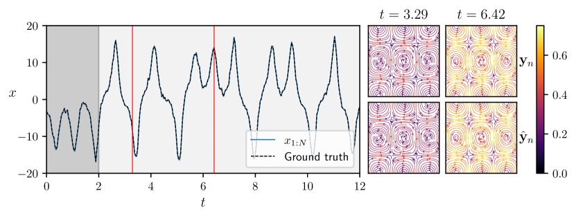
Figure 3: Left: Ground truth pseudo-observations (dashed) compared to encoding ${\mathbf{x}}_{1:N}\sim q_{\phi^{\star}}(\cdot|{\mathbf{y}}_{1:N})$ (solid). Training data indicated by grey-fill ($t=\left[0,2\right)$), red lines indicate reconstruction times. Right: Observed data ${\mathbf{y}}_{n}$ plotted alongside reconstructions $\hat{{\mathbf{y}}}_{n}$, with the velocity field shown as a streamplot where the color indicates the speed of the flow.

Results for the estimation of parameter $\sigma$ during the joint training are given in Fig. 4(a). The variational distribution is initialised at the prior $q_{\lambda_{0}}({\mathbf{\Lambda}})=\mathcal{N}(30,5^{2})$, and over the joint training period the mean converges on the true value $\sigma=10$, and the variance reduces and appears to level off. Fig. 4(b) shows the latent inference for the full dataset, the first column shows the distribution $p({\mathbf{u}}_{n}|{\mathbf{x}}_{1:n},{\mathbf{\Lambda}})$, with sampled ${\mathbf{x}}_{1:n}\sim q_{\phi^{\star}}(\cdot|{\mathbf{y}}_{1:N})$ and ${\mathbf{\Lambda}}\sim q_{\lambda^{\star}}(\cdot)$ which shows good correspondence to the true latent values. The third column shows the mixture of Gaussian approximation to $p({\mathbf{u}}_{n}|{\mathbf{y}}_{1:n})$ (see Eq. 4.2), with the second column visualising the individual mixture components. As expected, the observed latent dimension $u_{1}$ has a smaller variance than the unobserved components $u_{2},u_{3}$, with low bias seen for all three dimensions.

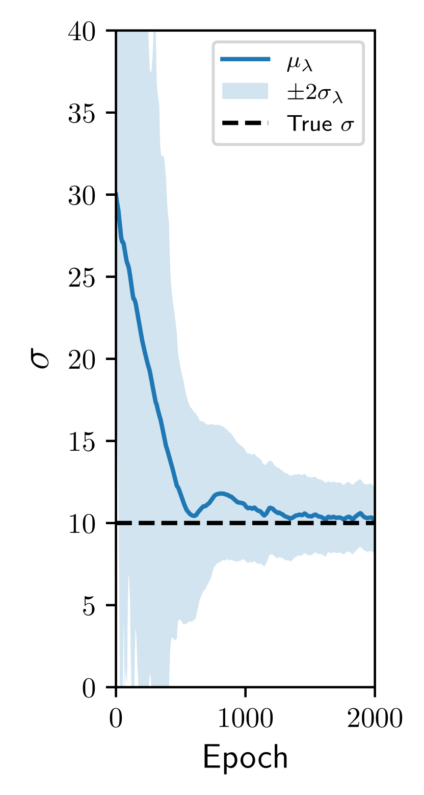
(a)

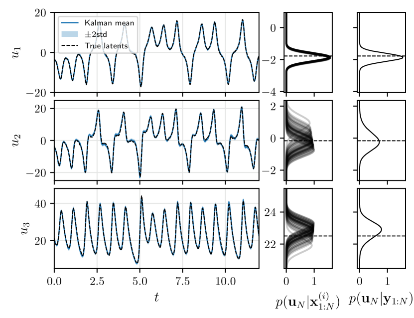
(b)

Figure 4: Inference results for $\Phi$-DVAE jointly trained on Lorenz-63 system. (a) Trace plot of parameter variational distribution $q_{\lambda}({\mathbf{\Lambda}})=\mathcal{N}(\mu_{\lambda},\sigma_{\lambda}^{2})$, with mean (blue) and $\pm 2$ standard deviations (blue fill). Initialised at poorly specified prior, $p({\mathbf{\Lambda}})=\mathcal{N}(30,5^{2})$. True value $\sigma=10$ (dashed). (b) First column: Filtering inference for latent states ${\mathbf{u}}_{1:N}$, where the filtering distribution $p({\mathbf{u}}_{n}|{\mathbf{x}}_{1:n})$ is plotted with the ground truth ${\mathbf{u}}^{\text{true}}_{n}$. Second column: Final-time filtering distribution $p({\mathbf{u}}_{N}|{\mathbf{x}}_{1:N}^{(i)})$, for multiple samples ${\mathbf{x}}_{1:N}^{(i)},i=1,\dots,50$. Third column: Mixture of Gaussians distribution, $p({\mathbf{u}}_{N}|{\mathbf{y}}_{1:N})$, calculated via Eq. 4.2. True latent values ${\mathbf{u}}_{N}^{\text{true}}$ shown as horizontal dashed lines.

Fig. 5 shows the results of the predictive rollout. In this scenario, the training data is encoded from $t=0$ to $t=2$, and the latent states are predicted ahead in time by iterating Eq. 6 until $t=4.5$.

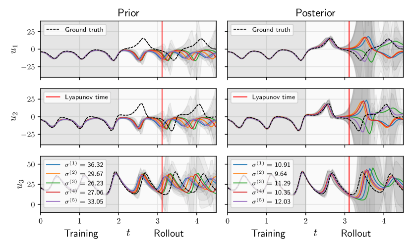
Figure 5: Training time indicated with grey-fill $t=\left[0,2\right)$, and rollout time from $t=\left[2,4.5\right]$. Filtering distributions $p({\mathbf{u}}_{n}|{\mathbf{x}}_{1:n}^{(i)},{\mathbf{\Lambda}}^{(i)})=\mathcal{N}({\mathbf{m}}_{n}^{(i)},{\mathbf{C}}_{n}^{(i)})$ visualised with ${\mathbf{m}}_{n}^{(i)}$ (solid) and $\pm 2$ standard deviations computed from ${\mathbf{C}}_{n}^{(i)}$ (grey-bands), alongside the true latents ${\mathbf{u}}_{1:N}^{\text{true}}$ (dashed). First column: samples generated by the prior model, ${\mathbf{x}}_{1:N}^{(i)}\sim q_{\phi}(\cdot|{\mathbf{y}}_{1:N})$, ${\mathbf{\Lambda}}^{(i)}\sim p(\cdot)$. Second column: samples generated from the posterior model, ${\mathbf{x}}_{1:N}^{(i)}\sim q_{\phi^{\star}}(\cdot|{\mathbf{y}}_{1:N})$, ${\mathbf{\Lambda}}^{(i)}\sim q_{\lambda^{\star}}(\cdot)$.

The predictive variance for each sample is displayed as a $\pm 2$ standard deviation fill for each sample. For reference, the Lyapunov time for the deterministic latent system with the ground truth parameters is shown as a red vertical bar. This indicates the time for which prediction should be possible for the chaotic system [75, 76]. The latent predictions from the misspecified prior model rapidly diverge from the true latent state. In comparison, the posterior predictions successfully track the latent state up until the Lyapunov time, where predictions become uncertain and begin to diverge as expected. It should be noted the prior model is misspecified in the sense that the prior mean produces a non-chaotic system, with most of the probability mass concentrated on non-chaotic systems.

5.2 Advection PDE

As a second example, we consider the advection equation with periodic boundary conditions. In this example, we derive the transition density $p({\mathbf{u}}_{n}|{\mathbf{u}}_{n-1},{\mathbf{\Lambda}})$ from a statFEM discretisation of a stochastic advection equation:

$$\partial_{t}u+c\,\partial_{s}u=\dot{\xi},\quad\dot{\xi}\sim\mathcal{GP}(0,\delta(t-t^{\prime})\cdot k(s,s^{\prime})),$$ (8)

where $u:=u(s,t)$, $\xi:=\xi(s,t)$, $s\in[0,1]$, $t\in[0,40]$, and $u(s,t)=u(s+1,t)$. Recall that, as in Section 3.2, the FEM coefficients ${\mathbf{u}}_{n}=(u_{1}(n\Delta_{t}),\ldots,u_{n_{u}}(n\Delta_{t}))$ are the latent variables. These are related to the discretised solution via $u_{h}(s,n\Delta_{t})=\sum_{i=1}^{n_{u}}u_{i}(n\Delta_{t})\phi_{i}(s)$ (see A and C).

Video data ${\mathbf{y}}_{1:N}$ is generated from the deterministic version of (8) (i.e. (8) with $\xi\equiv 0$). Since the solution of this equation is available analytically, we use this for data generation. Denoting the initial condition $f(s)=u(s,0)$, the solution to  (8) at a time $t$ is given by $u(s,t)=f(s-ct)$. This trajectory is evaluated at discrete time points $\left\{n\Delta_{t}\right\}_{n=1}^{N}$ and the solutions $u(s,n\Delta_{t})$ are imposed onto a 2D grid. On the grid, pixels below $u(s,n\Delta_{t})$ are lit-up in a binary fashion, along with salt-and-pepper noise [77]. In this experiment we use fixed parameters, setting the wavespeed $c=0.5$. We set the decoder as $p_{\theta}({\mathbf{y}}_{n}|{\mathbf{x}}_{n})=\mathrm{Bern}(f_{\theta}({\mathbf{x}}_{n}))$ and the encoder as $q_{\phi}({\mathbf{x}}_{n}|{\mathbf{y}}_{n})={\mathcal{N}}(\mu_{\phi}({\mathbf{y}}_{n}),\sigma_{\phi}({\mathbf{y}}_{n}))$. As previous, see A for full details.

Due to linearity of the underlying dynamical system, we compare the $\Phi$-DVAE to the KVAE for a set of video data generated from the advection equation, for various dimensions of the KVAE latent space. Specifying a particular form of PDE dynamics on the latent states increases the inductive bias imposed on the latent space, and should provide better reconstructions and higher likelihood of the data. We choose two metrics to evaluate this: the ELBO given by $\log p_{\theta}({\mathbf{y}}_{1:N}|{\mathbf{x}}_{1:N})-\log q_{\phi}({\mathbf{x}}_{1:N}|{\mathbf{y}}_{1:N})+\log p({\mathbf{x}}_{1:N})$, and the normalised mean-squared-error (MSE) of reconstruction compared to the noise-free video frames, ${\mathbf{y}}_{1:N}^{\text{true}}$. The normalised MSE is given by $\|{\mathbf{y}}_{1:N}^{\text{true}}-\hat{{\mathbf{y}}}_{1:N}\|_{2}^{2}/\|{\mathbf{y}}_{1:N}^{\text{true}}\|_{2}^{2}$. We compare our method to KVAE for the linear advection example for varying latent dimension of the KVAE, and the results are plotted in Fig. 6. We also include the results for our method but with deterministic latent transitions (${\mathbf{Q}}=\mathbf{0}$) to assess the impact of accounting for misspecification through the use of statFEM.

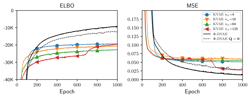
Figure 6: Comparison of KVAE and $\Phi$-DVAE for the advection equation.

From Fig. 6, $\Phi$-DVAE outperforms each KVAE model, with a larger ELBO and smaller normalised MSE during training. The MSE for the $\Phi$-DVAE model is 1.26%, compared to the best KVAE model ($n_{x}=128$) with 2.71%, where roughly a 5% normalised MSE is considered a good reconstruction. The KVAE models performed similarly in terms of ELBO, with dimension 4 and 128 the best with -19273 and -19659 respectively, but are outperformed by both $\Phi$-DVAE models. We also note that including the process noise matrix ${\mathbf{Q}}$ for the statFEM model which accounts for misspecification outperforms the model that evolves the latent states deterministically.

5.3 Korteweg–de Vries PDE

As previously, the latent transition density $p({\mathbf{u}}_{n}|{\mathbf{u}}_{n-1},{\mathbf{\Lambda}})$ defines the evolution of the FEM coefficients, as given by a statFEM discretisation of a stochastic KdV equation:

$$\partial_{t}u+\alpha u\partial_{s}u+\beta\partial_{s}^{3}u+\nu u=\dot{\xi},\quad\dot{\xi}\sim\mathcal{GP}(0,\delta(t-t^{\prime})\cdot k(s,s^{\prime})),$$

where $u:=u(s,t)$, $\xi:=\xi(s,t)$, $s\in[0,2]$, $t\in[0,1]$, and $u(s,t)=u(s+2,t)$. We set the coefficients $\alpha=1,\beta=0.022^{2}$, and we investigate two cases, one with and one without drag ($\nu=0,\nu=1$). The initial condition is set to $u_{h}^{\mathrm{true}}(s,0)=\cos(\pi s)$ as in the classical work of Zabusky and Kruskal [78]. This regime is characterised by the steepening of the initial condition and the generation of solitons; nonlinear waves which have particle-like interactions [64].

Data is generated by simulating a trajectory ${\mathbf{u}}_{1:N}^{\mathrm{true}}$ using a FEM discretisation of the deterministic KdV equation and we impose FEM solutions $u_{h}^{\mathrm{true}}(s,n\Delta_{t})$ on a 2D grid. We light up pixels below the solution, which mimics an experimental setup where the wave-profile is recorded side-on. Independent salt-and-pepper noise is added onto each image frame. We set the decoder as $p_{\theta}({\mathbf{y}}_{n}|{\mathbf{x}}_{n})=\mathrm{Bern}(\mu_{\theta}({\mathbf{x}}_{n}))$ and the encoder as $q_{\phi}({\mathbf{x}}_{n}|{\mathbf{y}}_{n})={\mathcal{N}}(\mu_{\phi}({\mathbf{y}}_{n}),\sigma_{\phi}({\mathbf{y}}_{n}))$; see A for details.

KdV Results

The aim of this experiment is to learn the mapping from image frames to the latent observations, which we approximate with a neural network as described in Section 4. Additionally, we wish to estimate the posterior distribution over the unknown drag coefficient $\nu$, for both with drag ($\nu=1$) and without ($\nu=0$). The prior distribution $p(\nu)$ (with ${\mathbf{\Lambda}}=\left\{\nu\right\}$) implicitly places a prior over a family of KdV PDEs with varying drag coefficients. Since this physical coefficient is positively constrained, we reflect this in the choice of prior such that $\text{supp}(p(\nu))=\mathbb{R}^{+}$. For $\nu=1$ we use a log-normal prior distribution, and log-normal variational approximation, which we denote by $p(\nu)=\mathcal{LN}(\mu_{0},\sigma_{0}^{2})$, $q_{\lambda}(\nu)=\mathcal{LN}(\mu_{\lambda},\sigma_{\lambda}^{2})$ respectively. For the no-drag case ($\nu=0$), we use the exponential distribution for both prior and variational approximation, denoted by $p(\nu)=\text{Exp}(\lambda_{0})$ and $q_{\lambda}(\nu)=\text{Exp}(\lambda)$ respectively. For both cases, the choice of prior/posterior pairs provide analytic KL-divergences (see Table 1) for use in the ELBO computation. Following the Lorenz63 example, the variational approximations are initialised at poorly specified priors to assess the model’s ability to correct for this misspecification.

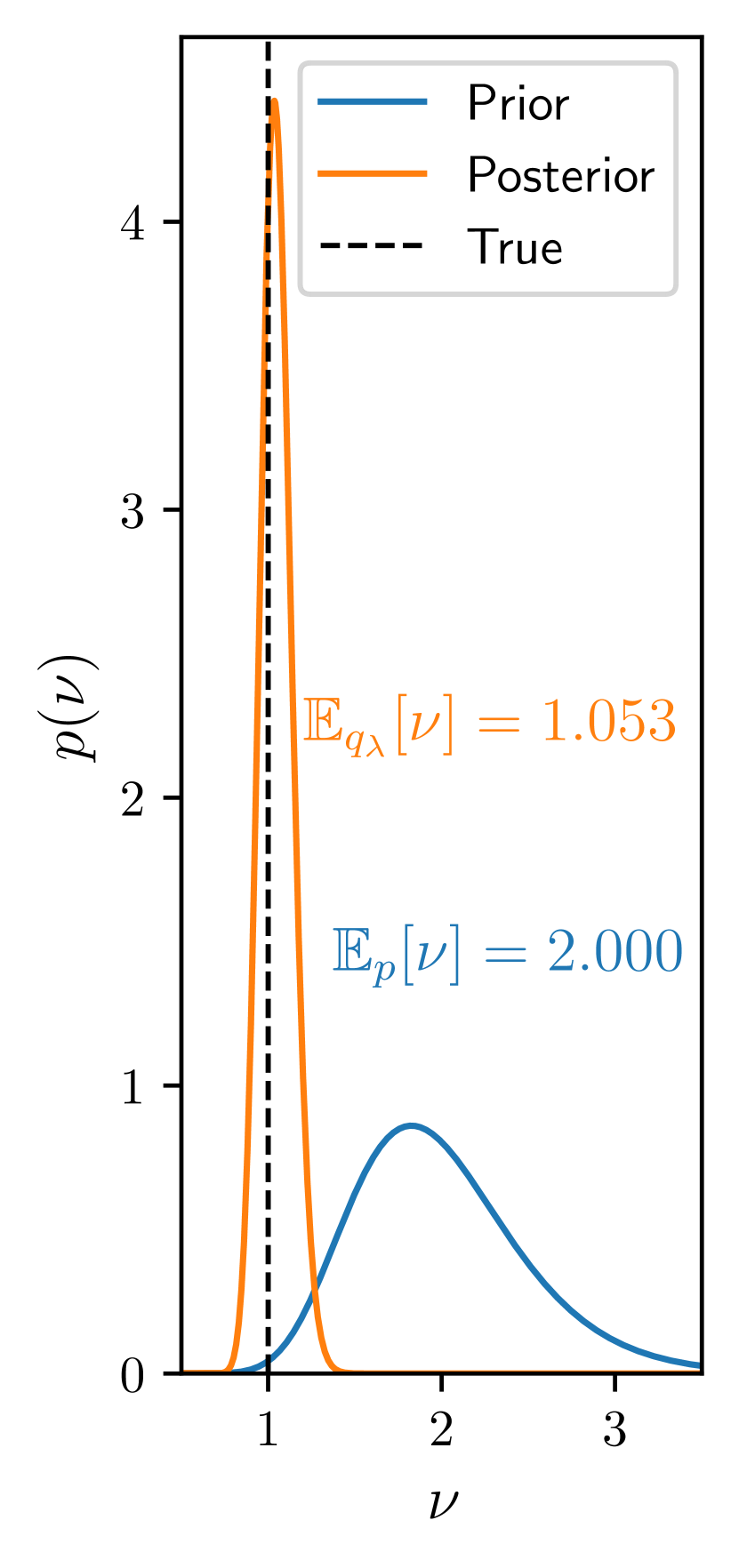
(a)

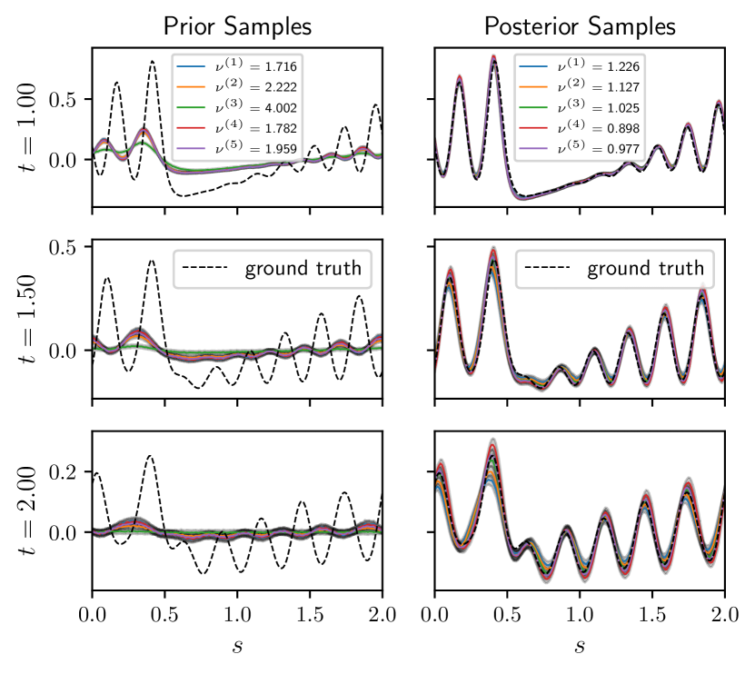
(b)

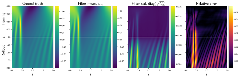
(c)

Figure 7: Inference results for KdV with drag. (a) Comparison of prior and variational posterior for model parameter $\nu=1$. (b) Latent filtering distribution shown for prior and posterior model for multiple samples. Prior model: $\left\{\phi,\theta\right\}$ trained using ${\mathbf{\Lambda}}\sim p(\nu)$. Posterior model: $\left\{\phi^{\star},\theta^{\star},\lambda^{\star}\right\}$ trained using ${\mathbf{\Lambda}}\sim q_{\lambda}(\nu)$. (c) Rollout prediction. The values of the latent process are shown in space (horizontal axis) and time (vertical axis). Rollout begins at $t=1.0$ (horizontal white line). Relative error: $|{\mathbf{u}}_{n}-{\mathbf{u}}_{n}^{\text{true}}|/\max_{1\leq i\leq n_{u}}|u_{i,n}^{\text{true}}|$.

(a)

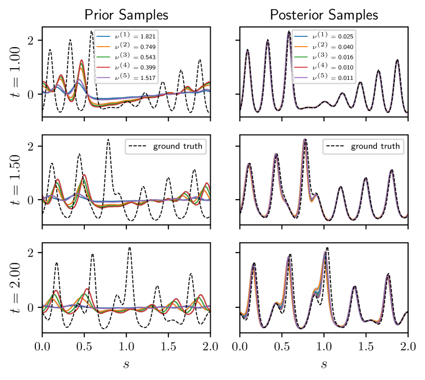
(b)

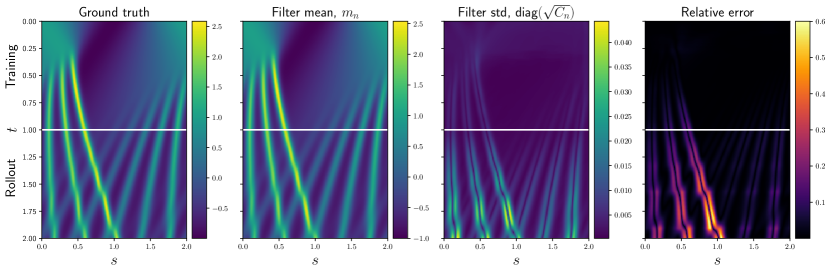
(c)

Figure 8: Inference results for no-drag KdV. (a) Comparison of prior and variational posterior for model parameter $\nu=0$. (b) Latent filtering distribution shown for prior and posterior model for multiple samples. Prior model: $\left\{\phi,\theta\right\}$ trained using ${\mathbf{\Lambda}}\sim p(\nu)$. Posterior model: $\left\{\phi^{\star},\theta^{\star},\lambda^{\star}\right\}$ trained using ${\mathbf{\Lambda}}\sim q_{\lambda}(\nu)$. (c) Rollout prediction. The values of the latent process are shown in space (horizontal axis) and time (vertical axis). Rollout begins at $t=1.0$ (horizontal white line). Relative error: $|{\mathbf{u}}_{n}-{\mathbf{u}}_{n}^{\text{true}}|/\max_{1\leq i\leq n_{u}}|u_{i,n}^{\text{true}}|$.

KdV with drag  For $\nu=1$, we set the prior $p(\nu)=\mathcal{LN}(2,0.5^{2})$ and show this alongside the posterior estimate in Fig. 7(a). The posterior has contracted around the true value. Fig. 7(b) shows the latent inference at specific time-points for multiple samples from both the prior and posterior, showing the improvement of the model when adapting the variational posterior jointly with the encoder. Marginalising over the parameter $\nu$ using samples from the posterior approximation $q_{\lambda^{\star}}(\nu)$ allow us to investigate the effect of uncertainty on the parameter estimate. These samples show a spread in mean estimates where the solitons are mixing at time $t=2.5$; the amplitude here is sensitive to changes in the drag coefficient, which is reflected in the variation of the filtering posterior samples. Fig. 7(c) shows the resulting inference and rollout for the jointly trained encoder $\phi^{\star}$ and sample from the posterior $q_{\lambda^{\star}}(\nu)$. The relative error is computed by normalising the absolute error by the max absolute value of the true solution at each time point, which accounts for the reduction in amplitude of the solution through time so that the growth in relative error can be observed. The latent mean is visualised alongside the ground truth, with the relative error. The relative error is low for the training time, and steadily increasing during rollout. Visualisation of the uncertainty is provided by the standard deviation of each latent dimension through time. The structure of the uncertainty is consistent with the relative error. We note that when initialised with a prior over $\nu$ centered on a much less dissipative system, the model struggles to adjust the posterior to a more dissipative system. We believe that since the pre-training on a less dissipative system produces latents that are more separated on the latent space, the autoencoder is able to still able to reconstruct the video frames due to the flexibility of the NN decoder. For these results, the system is initialised with a large drag coefficient, and early stopping used for regularisation.

No-drag KdV  For $\nu=0$, we set the prior $p(\nu)=\text{Exp}(1.0)$ and show this alongside the posterior estimate in Fig. 8(a). The posterior $q_{\lambda}(\nu)=\text{Exp}(62.2)$ places more density on the true value, $q_{\hat{\lambda}}(0)>p(0)$, and the resulting latent inference shows the comparison to the prior (see Fig. 8(b)). Whilst the posterior shows an improved fit to the true latents compared to the prior, there is still a clear mismatch. For $t=1$ when the rollout begins, the solitons of the latent samples appear out of phase with the true solution, which causes a mismatch when predicted forward in time. There is also a bias due to the parameter samples being non-zero, and hence predictions begin to diverge from the true solution which does not dissipate. Fig. 8(c) shows the inference and rollout prediction. The predicted mean has the same structure as the true latents, and the covariance structure reflects the error in the mean.

6 Conclusions

In this work, we introduced the concept of unstructured data assimilation (UDA), where unstructured data is used for state and parameter inference in a known physics model. We proposed a dynamical autoencoder approach to address the UDA problem, and demonstrated the model on three differential equation systems. The model can accurately embed unstructured data into pseudo-observations of the known physical system, and recover the true latent state of the system by filtering the pseudo-observations with the extended Kalman filter (ExKF).

With the inclusion of prior knowledge on the physics, data-efficient learning is achieved. In particular, the extrapolation of the Lorenz-63 system to inferring unseen regions of the attractor based on $50$ velocity field observations, and the inversion of the KdV PDE with $100$ observed video frames. Accurate parameter estimation has also been demonstrated in both these examples, with the added benefit of parameter uncertainty quantification. We have shown the effect of maginalising out this uncertainty on the latent inference, which results in a mixture of Gaussians filtering distribution that is able to capture variation in the latent solution in areas that are sensitive to model parameters. Comparison of $\Phi$-DVAE was made to a baseline model, the KVAE. This showed our model performing better in terms of Bayesian model evidence and mean-squared-error of reconstruction due to the added inductive bias introduced by the known physical system, compared to an arbitrary learned linear Gaussian state-space model.

Our $\Phi$-DVAE model has demonstrated that state estimation and inversion are possible in the case of UDA, when carefully embedding knowledge about the underlying dynamical system. Further work could extend this methodology to include direct measurements, as well as the indirect, unstructured observations in order to augment the inference when direct measurements are sparse, or expensive.

Appendix A Numerical Details and Network Architectures

Lorenz-63 experiment.

• Time-series length: $N=300$. Training length: $50$, Test length: $250$

• Input: $n_{y}=200$.

• Pseudo-observations: $n_{x}=1$.

• Latent $n_{u}=3$.

• Decoder: $p_{{\mathbf{w}}}({\mathbf{y}}_{n}|x_{n})={\mathcal{N}}({\mathbf{w}}x_{n},\eta^{2}{\mathbf{I}})$, $\eta=0.1$.

• Encoder: $q_{{\mathbf{w}}}(x_{n}|{\mathbf{y}}_{n})={\mathcal{N}}(({\mathbf{w}}^{\top}{\mathbf{w}})^{-1}{\mathbf{w}}^{\top}{\mathbf{y}}_{n},\eta^{2}({\mathbf{w}}^{\top}{\mathbf{w}})^{-1})$

• Latent initial condition: ${\mathbf{u}}_{0}=\left[-3.7277,-3.8239,21.1507\right]^{\top}$

• Latent noise processes: ${\mathbf{L}}=\operatorname{diag}(1.0^{2})$, ${\mathbf{R}}=\operatorname{diag}(0.4^{2})$.

• Latent discretisation: Euler-Maruyama, $dt=0.001$.

• Model parameter prior: $p(\sigma)=\mathcal{N}(30,5^{2})$.

• Optimiser: Adam, learning rate = $10^{-2}$.

• Training Epochs: 2000.

To generate the data, we simulate the Lorenz SDE with $dt=0.001$ and take pseudo-observations $x_{n}$ every $40$ time-steps of the latent system, for a total of $N=300$ with $\Delta_{t}=0.04$. Velocity measurements are taken in the $s_{1}$ and $s_{2}$ directions over a regular $10\times 10$ grid on the domain $s_{1},s_{2}\in[-4,4]$, via the streamfunction $\psi(s_{1},s_{2},t)$. These measurements are flattened to the data vector ${\mathbf{y}}_{n}\in\mathbb{R}^{n_{y}}$, $n_{y}=200$. Parameters for data generation are ${\mathbf{\Lambda}}=\left\{\sigma=10,r=28,b=8/3\right\}$.

Advection equation experiment.

• Time-series length: $N=200$.

• Input: $n_{y}=784$.

• Pseudo-observations: $n_{x}=64$.

• Latent $n_{u}=64$.

• Decoder: $p_{\theta}({\mathbf{y}}_{n}|{\mathbf{x}}_{n})=\text{Bern}(\mu_{\theta}({\mathbf{x}}_{n}))$

• $\mu_{\theta}(\cdot)$: MLP, two fully connected hidden layers with dimension 128

• Encoder: $q_{\phi}({\mathbf{x}}_{n}|{\mathbf{y}}_{n})={\mathcal{N}}(\mu_{\phi}({\mathbf{y}}_{n}),\sigma_{\phi}({\mathbf{y}}_{n}))$

• $\mu_{\phi}(\cdot),\log\sigma_{\phi}(\cdot)$: MLP, two fully connected hidden layers with dimension 128

• Neural Network activations: LeakyReLU, negative slope $=0.01$

• Latent initial condition: $u(s,0)=\exp(-2(s-2.5)^{2}),s\in[0,5]$.

• Latent noise processes: $\rho=0.1$, $\ell=0.1$, ${\mathbf{R}}=\operatorname{diag}(0.1^{2})$.

• Latent discretisation: FEM, $C^{0}([0,1])$ polynomial trial/test functions, Crank-Nicolson time discretisation, $dt=0.02$.

• Optimiser: Adam, learning rate = $0.001$.

• Salt-and-pepper noise, probability of pixel information loss: $0.02$

To generate the data, we evaluate the analytical solution at every $dt=0.02$, taking pseudo-observations every 10 time-steps for $\Delta_{t}=0.2$ and $N=200$. Latent dimensions are $n_{u}=64$ and $n_{x}=64$, with each image $28\times 28$ pixels. These images are then flattened to vectors ${\mathbf{y}}_{n}\in\left[0,1\right]^{n_{y}}$, with $n_{y}=784$.

KdV equation experiment.

• Time-series length: $N=100$.

• Input: $n_{y}=1792$.

• Pseudo-observations: $n_{x}=40$.

• Latent $n_{u}=600$.

• Decoder: $p_{\theta}({\mathbf{y}}_{n}|{\mathbf{x}}_{n})=\text{Bern}(S(f_{\theta}({\mathbf{x}}_{n})))$

• $f_{\theta}(\cdot)$: MLP, three fully connected hidden layers with dimension 128

• Encoder: $q_{\phi}({\mathbf{x}}_{n}|{\mathbf{y}}_{n})={\mathcal{N}}(\mu_{\phi}({\mathbf{y}}_{n}),\sigma_{\phi}({\mathbf{y}}_{n}))$

• $\mu_{\phi}(\cdot),\log\sigma_{\phi}(\cdot)$: MLP, three fully connected hidden layers with dimension 128

• Neural Network activations: tanh

• Fixed parameters: $\alpha=1.0,\beta=0.022^{2}$

• Unknown parameter (with drag): $\nu=1.0$.

• Unknown parameter (no-drag): $\nu=0$.

• Latent initial condition: $u(s,0)=\cos(\pi s),s\in[0,2]$.

• Latent noise processes: $\rho=0.01$, $\ell=0.2$, ${\mathbf{R}}=\operatorname{diag}(0.02^{2})$.

• Latent discretisation: Petrov-Galerkin approach of Debussche and Printems [79]: $C^{0}([0,2])$ polynomial trial functions, Crank-Nicolson time discretisation, $dt=0.01$.

• Parameter prior (with drag): $p({\mathbf{\Lambda}})=\mathcal{LN}(2,0.5^{2})$.

• Parameter prior (no-drag): $p({\mathbf{\Lambda}})=\text{Exp}(1.0)$.

• Optimiser: Adam, learning rate = $0.005$.

• Salt-and-pepper noise, probability of pixel information loss: $0.02$

To generate the data we simulate the KdV equation with a high-fidelity in space and time to ensure accurate latent data, and avoid inverse crimes. For the data used in comparison, we subsample this simulation with $dt=0.01$, observing every timestep for $\Delta_{t}=0.01$, and we take $N=100$ observations ${\mathbf{y}}_{n}$, with ${\mathbf{y}}_{n}\in\left[0,1\right]^{n_{y}}$. Each ${\mathbf{y}}_{n}$ is a flattened image of dimension $n_{y}=64\times 28=1792$, and we encode to pseudo-observations ${\mathbf{x}}_{n}$ of dimension $n_{x}=40$. The latent state dimension is $n_{u}=600$.

Neural network decoding/encoding.  Variational autoencoders use neural networks to parameterise the encoding distribution $q_{\phi}({\mathbf{x}}|{\mathbf{y}})$, and the probablisitic decoder $p_{\theta}({\mathbf{y}}|{\mathbf{x}})$. A common choice of variational distribution is the Gaussian, which uses a NN to parameterise the mean $\mu_{\phi}({\mathbf{y}})$, where $\mu_{\phi}\colon{\mathbb{R}}^{n_{y}}\to{\mathbb{R}}^{n_{x}}$, and another to parametrise the diagonal of the covariance. Parameterising the log-variance allows for both positive and negative neural network output — the values are exponentiated to calculate the positively constrained variances.

$$q_{\phi}({\mathbf{x}}|{\mathbf{y}})=\mathcal{N}\left(\mu_{\phi}({\mathbf{y}}),\text{diag}(\sigma_{\phi}({\mathbf{y}}))\right)$$

The decoder attempts to reconstruct the original data ${\mathbf{y}}$ from the latents ${\mathbf{x}}$. A NN decoder maps the latents to a reconstruction $\hat{{\mathbf{y}}}=f_{\theta}({\mathbf{x}})$, where $f_{\theta}\colon{\mathbb{R}}^{n_{x}}\to{\mathbb{R}}^{n_{y}}$ is the NN mapping parameterised by $\theta$. The probabilistic decoder depends on the form of the data. In this work, we use a Gaussian distribution for the velocity field data, and a Bernoulli distribution for the video data. When reconstructing video frames, an element-wise sigmoid function is used as the final layer of the neural network, in order to output grayscale pixel values, i.e. $S(y)=1/(1+\exp(-y))$, where $S\colon{\mathbb{R}}^{n_{y}}\to\left[0,1\right]^{n_{y}}$. The two examples of unstructured data, real-valued velocity field data, and binary pixel data can be reconstructed as follows:
Real-valued data, ${\mathbf{y}}\in{\mathbb{R}}^{n_{y}}$, we reconstruct $\hat{{\mathbf{y}}}\in{\mathbb{R}}^{n_{y}}$, where $\hat{{\mathbf{y}}}=f_{\theta}({\mathbf{x}})$. Often in practice an independent noise model is used, with standard deviation $\sigma$, giving the density and log-density as follows:

$$p_{\theta}({\mathbf{y}}|{\mathbf{x}}) =\mathcal{N}\left({\mathbf{y}};\hat{{\mathbf{y}}},\sigma^{2}{\mathbf{I}}\right)$$

$$\log p_{\theta}({\mathbf{y}}|{\mathbf{x}}) =-n_{y}\log(2\pi\sigma^{2})-\left\|{\mathbf{y}}-\hat{{\mathbf{y}}}\right\|_{2}^{2}$$

Binary pixel data, ${\mathbf{y}}\in\left\{0,1\right\}^{n_{y}}$ we reconstruct $\hat{{\mathbf{y}}}\in\left[0,1\right]^{n_{y}}$, where $\hat{{\mathbf{y}}}=S\left(f_{\theta}({\mathbf{x}})\right)$. The density and log-density are given as follows:

$$p_{\theta}({\mathbf{y}}|{\mathbf{x}}) =\text{Bern}\left({\mathbf{y}};\hat{{\mathbf{y}}}\right)$$

$$\log p_{\theta}({\mathbf{y}}|{\mathbf{x}}) =\sum_{i=1}^{n_{y}}y_{i}\log(\hat{y}_{i})+(1-y_{i})\log(1-\hat{y}_{i})$$

Linear decoding/encoding.  Unlike the nonlinear NN decoders, if linear data generation is assumed from ${\mathbf{x}}$ to ${\mathbf{y}}$, we can invert this in order to encode our data. With a linear decoder of the form:

$$p_{{\mathbf{A}}}({\mathbf{y}}|{\mathbf{x}})=\mathcal{N}({\mathbf{A}}{\mathbf{x}},\eta^{2}I).$$

In this case, we use the “inverted” linear decoder given by:

$$q_{{\mathbf{A}}}({\mathbf{x}}|{\mathbf{y}})=\mathcal{N}(({\mathbf{A}}^{\top}{\mathbf{A}})^{-1}{\mathbf{A}}^{\top}{\mathbf{y}},\eta^{2}({\mathbf{A}}^{\top}{\mathbf{A}})^{-1}).$$

By selecting the encoder appropriately, the space of parameterised variational distributions can be restricted to align with our beliefs about the data generation process.

Appendix B Full Variational Framework

We derive the approximate ELBO for joint estimation of dynamic parameters ${\mathbf{\Lambda}}$, and autoencoder parameters $\phi,\theta$. We start by writing the evidence

$$p({\mathbf{y}}_{1:N})=\int p({\mathbf{u}}_{1:N},{\mathbf{x}}_{1:N},{\mathbf{\Lambda}},{\mathbf{y}}_{1:N}){\mathrm{d}}{\mathbf{x}}_{1:N}{\mathrm{d}}{\mathbf{u}}_{1:N}{\mathrm{d}}{\mathbf{\Lambda}}.$$

We maximise $\log p({\mathbf{y}}_{1:N})$ as

$$\log p({\mathbf{y}}_{1:N}) =\log\int p({\mathbf{u}}_{1:N},{\mathbf{x}}_{1:N},{\mathbf{\Lambda}},{\mathbf{y}}_{1:N}){\mathrm{d}}{\mathbf{x}}_{1:N}d{\mathbf{u}}_{1:N}{\mathrm{d}}{\mathbf{\Lambda}}$$

$$=\log\int\frac{p({\mathbf{u}}_{1:N},{\mathbf{x}}_{1:N},{\mathbf{\Lambda}},{\mathbf{y}}_{1:N})}{q({\mathbf{u}}_{1:N},{\mathbf{x}}_{1:N},{\mathbf{\Lambda}}|{\mathbf{y}}_{1:N})}q({\mathbf{u}}_{1:N},{\mathbf{x}}_{1:N},{\mathbf{\Lambda}}|{\mathbf{y}}_{1:N}){\mathrm{d}}{\mathbf{x}}_{1:N}{\mathrm{d}}{\mathbf{u}}_{1:N}{\mathrm{d}}{\mathbf{\Lambda}}$$

$$\geq\int\log\left[\frac{p({\mathbf{u}}_{1:N},{\mathbf{x}}_{1:N},{\mathbf{\Lambda}},{\mathbf{y}}_{1:N})}{q({\mathbf{u}}_{1:N},{\mathbf{x}}_{1:N},{\mathbf{\Lambda}}|{\mathbf{y}}_{1:N})}\right]q({\mathbf{u}}_{1:N},{\mathbf{x}}_{1:N},{\mathbf{\Lambda}}|{\mathbf{y}}_{1:N}){\mathrm{d}}{\mathbf{x}}_{1:N}{\mathrm{d}}{\mathbf{u}}_{1:N}{\mathrm{d}}{\mathbf{\Lambda}}$$

$$=\text{ELBO},$$

where the third line follows from the application of Jensen’s inequality. Our generative model determines the factorisation of the joint distribution, given in (1):

$$p({\mathbf{u}}_{1:N},{\mathbf{x}}_{1:N},{\mathbf{\Lambda}},{\mathbf{y}}_{1:N}) =p({\mathbf{y}}_{1:N}|{\mathbf{x}}_{1:N},{\mathbf{u}}_{1:N},{\mathbf{\Lambda}})p({\mathbf{x}}_{1:N}|{\mathbf{u}}_{1:N},{\mathbf{\Lambda}})p({\mathbf{u}}_{1:N}|{\mathbf{\Lambda}})p({\mathbf{\Lambda}})$$

$$=p_{\theta}({\mathbf{y}}_{1:N}|{\mathbf{x}}_{1:N})p({\mathbf{x}}_{1:N}|{\mathbf{u}}_{1:N},{\mathbf{\Lambda}})p({\mathbf{u}}_{1:N}|{\mathbf{\Lambda}})p({\mathbf{\Lambda}}).$$

Next, we plug this factorised distribution into the ELBO and obtain

$$\text{ELBO}=\int\log\left[\frac{p_{\theta}({\mathbf{y}}_{1:N}|{\mathbf{x}}_{1:N})p({\mathbf{x}}_{1:N}|{\mathbf{u}}_{1:N},{\mathbf{\Lambda}})p({\mathbf{u}}_{1:N}|{\mathbf{\Lambda}})p({\mathbf{\Lambda}})}{q({\mathbf{u}}_{1:N},{\mathbf{x}}_{1:N},{\mathbf{\Lambda}}|{\mathbf{y}}_{1:N})}\right]\times q({\mathbf{u}}_{1:N},{\mathbf{x}}_{1:N},{\mathbf{\Lambda}}|{\mathbf{y}}_{1:N})\,{\mathrm{d}}{\mathbf{x}}_{1:N}{\mathrm{d}}{\mathbf{u}}_{1:N}{\mathrm{d}}{\mathbf{\Lambda}}.$$

The family of distributions which we use to approximate the posterior is described below. We assume a factorisation based on the model into variational encoding $q_{\phi}(\cdot)$, a full latent state posterior $q_{\nu}(\cdot)$, and the variational approximation to the parameter posterior $q_{\lambda}(\cdot)$:

$$q({\mathbf{u}}_{1:N},{\mathbf{x}}_{1:N},{\mathbf{\Lambda}}|{\mathbf{y}}_{1:N}) =q({\mathbf{u}}_{1:N}|{\mathbf{x}}_{1:N},{\mathbf{\Lambda}})q_{\lambda}({\mathbf{\Lambda}})q_{\phi}({\mathbf{x}}_{1:N}|{\mathbf{y}}_{1:N})$$

$$=q({\mathbf{u}}_{1:N}|{\mathbf{x}}_{1:N},{\mathbf{\Lambda}})q_{\lambda}({\mathbf{\Lambda}})\prod_{n=1}^{N}q_{\phi}({\mathbf{x}}_{n}|{\mathbf{y}}_{n}).$$

The second line demonstrates the amortized structure of the autoencoder, where the same encoding parameters are shared across datapoints. We can then substitute this expression into our ELBO and obtain

$$\text{ELBO}=\int\log\left[\frac{p_{\theta}({\mathbf{y}}_{1:N}|{\mathbf{x}}_{1:N})p({\mathbf{x}}_{1:N}|{\mathbf{u}}_{1:N},{\mathbf{\Lambda}})p({\mathbf{u}}_{1:N}|{\mathbf{\Lambda}})p({\mathbf{\Lambda}})}{q({\mathbf{u}}_{1:N}|{\mathbf{x}}_{1:N},{\mathbf{\Lambda}})q_{\lambda}({\mathbf{\Lambda}})q_{\phi}({\mathbf{x}}_{1:N}|{\mathbf{y}}_{1:N})}\right]\times q({\mathbf{u}}_{1:N}|{\mathbf{x}}_{1:N},{\mathbf{\Lambda}})q_{\lambda}({\mathbf{\Lambda}})q_{\phi}({\mathbf{x}}_{1:N}|{\mathbf{y}}_{1:N}){\mathrm{d}}{\mathbf{x}}_{1:N}{\mathrm{d}}{\mathbf{u}}_{1:N}{\mathrm{d}}{\mathbf{\Lambda}}.$$

Assuming the variational posterior is the exact filtering posterior, i.e., $q({\mathbf{u}}_{1:N}|{\mathbf{x}}_{1:N},{\mathbf{\Lambda}})=p({\mathbf{u}}_{1:N}|{\mathbf{x}}_{1:N},{\mathbf{\Lambda}})$ then applying Bayes rule

$$\frac{p({\mathbf{x}}_{1:N}|{\mathbf{u}}_{1:N},{\mathbf{\Lambda}})p({\mathbf{u}}_{1:N}|{\mathbf{\Lambda}})}{q({\mathbf{u}}_{1:N}|{\mathbf{x}}_{1:N},{\mathbf{\Lambda}})}=p({\mathbf{x}}_{1:N}|{\mathbf{\Lambda}})$$

leads to a simplification of ELBO in terms of the marginal likelihood $p({\mathbf{x}}_{1:N}|{\mathbf{\Lambda}})$ of the state-space model. Substituting this expression leads to

ELBO $$=\int\log\left[\frac{p_{\theta}({\mathbf{y}}_{1:N}|{\mathbf{x}}_{1:N})p({\mathbf{x}}_{1:N}|{\mathbf{\Lambda}})p({\mathbf{\Lambda}})}{q_{\phi}({\mathbf{x}}_{1:N}|{\mathbf{y}}_{1:N})q_{\lambda}({\mathbf{\Lambda}})}\right]$$

$$\quad\quad\quad\quad\times q({\mathbf{u}}_{1:N}|{\mathbf{x}}_{1:N},{\mathbf{\Lambda}})q_{\lambda}({\mathbf{\Lambda}})q_{\phi}({\mathbf{x}}_{1:N}|{\mathbf{y}}_{1:N}){\mathrm{d}}{\mathbf{x}}_{1:N}{\mathrm{d}}{\mathbf{u}}_{1:N}{\mathrm{d}}{\mathbf{\Lambda}}$$

$$=\int\log\left[\frac{p_{\theta}({\mathbf{y}}_{1:N}|{\mathbf{x}}_{1:N})}{q_{\phi}({\mathbf{x}}_{1:N}|{\mathbf{y}}_{1:N})}\right]q_{\phi}({\mathbf{x}}_{1:N}|{\mathbf{y}}_{1:N}){\mathrm{d}}{\mathbf{x}}_{1:N}$$

$$\quad\quad\quad\quad+\int\left[\log p({\mathbf{x}}_{1:N}|{\mathbf{\Lambda}})+\log\frac{p({\mathbf{\Lambda}})}{q_{\lambda}({\mathbf{\Lambda}})}\right]q_{\lambda}({\mathbf{\Lambda}})q_{\phi}({\mathbf{x}}_{1:N}|{\mathbf{y}}_{1:N}){\mathrm{d}}{\mathbf{x}}_{1:N}{\mathrm{d}}{\mathbf{\Lambda}}$$

$$=\mathbb{E}_{q_{\phi}}\left[\log\frac{p_{\theta}({\mathbf{y}}_{1:N}|{\mathbf{x}}_{1:N})}{q_{\phi}({\mathbf{x}}_{1:N}|{\mathbf{y}}_{1:N})}\right]+\mathbb{E}_{q_{\phi}}\left[\mathbb{E}_{q_{\lambda}}\left[\log p({\mathbf{x}}_{1:N}|{\mathbf{\Lambda}})+\log\frac{p({\mathbf{\Lambda}})}{q_{\lambda}({\mathbf{\Lambda}})}\right]\right]$$

$$=\mathbb{E}_{q_{\phi}}\left[\log\frac{p_{\theta}({\mathbf{y}}_{1:N}|{\mathbf{x}}_{1:N})}{q_{\phi}({\mathbf{x}}_{1:N}|{\mathbf{y}}_{1:N})}\right]+\mathbb{E}_{q_{\phi}}\left[\mathbb{E}_{q_{\lambda}}\left[\log p({\mathbf{x}}_{1:N}|{\mathbf{\Lambda}})\right]\right]-\operatorname{KL}(q_{\lambda}\;\|\;p).$$

Using a single MC samples ${\mathbf{x}}_{1:N}\sim q_{\phi}(\cdot|{\mathbf{y}}_{1:N})$, and ${\mathbf{\Lambda}}\sim q_{\lambda}(\cdot)$ to approximate the expectations, we can write the approximate ELBO, $\mathcal{L}(\phi,\theta,\lambda)$ as

$$\mathcal{L}(\theta,\phi,\lambda)=\log p_{\theta}({\mathbf{y}}_{1:N}|{\mathbf{x}}_{1:N})-\log q_{\phi}({\mathbf{x}}_{1:N}|{\mathbf{y}}_{1:N})+\log p({\mathbf{x}}_{1:N}|{\mathbf{\Lambda}})-\operatorname{KL}(q_{\lambda}\;\|\;p).$$

See Algorithm 1 for pseudo-code, and Table 1 for distributions that provide analytic KL-divergence.

Appendix C Further Details on the Dynamic Model

In this work we take the latent dynamical model to be a stochastic ODE or PDE. For an ODE this follows from a standard SDE [73], given by

$${\mathrm{d}}{\mathbf{u}}=f_{\Lambda}({\mathbf{u}},t;\Lambda){\mathrm{d}}t+{\mathbf{L}}(t){\mathrm{d}}{\mathbf{W}}(t),$$

where ${\mathbf{u}}:={\mathbf{u}}(t)\in{\mathbb{R}}^{n_{u}}$, $t\in[0,T]$, $f_{\Lambda}\colon{\mathbb{R}}^{n_{u}}\times[0,T]\to{\mathbb{R}}^{n_{u}}$, ${\mathbf{L}}\colon[0,T]\to{\mathbb{R}}^{n_{u}\times n_{u}}$. The noise process ${\mathbf{W}}(t)$ is a standard vector Brownian motion. The diffusion term ${\mathbf{L}}(t)$ can be used to describe any a priori correlation in the error process dimensions. As stated in the main text, this error process is taken to represent possibly misspecified/unknown physics, which may have been omitted when specifying the model. Discretisation with an explicit Euler-Maruyama scheme [72] gives,

$${\mathbf{u}}_{n}={\mathbf{u}}_{n-1}+\Delta_{t}f_{n-1}({\mathbf{u}}_{n-1};\Lambda)+{\mathbf{L}}_{n-1}\Delta{\mathbf{W}}_{n-1},\quad\Delta{\mathbf{W}}_{n-1}\sim{\mathcal{N}}(\bm{0},\Delta_{t}{\mathbf{I}}),$$

where ${\mathbf{u}}_{n}:={\mathbf{u}}(n\Delta_{t})$, $f_{n}(\cdot;\Lambda)=f_{\Lambda}(\cdot,n\Delta_{t})$, and so on. This gives a transition density

$$p({\mathbf{u}}_{n}|{\mathbf{u}}_{n-1},\Lambda)={\mathcal{N}}({\mathbf{u}}_{n-1}+\Delta_{t}f_{n-1}({\mathbf{u}}_{n-1};\Lambda),\Delta_{t}{\mathbf{L}}_{n-1}{\mathbf{L}}_{n-1}^{\top}),$$

defining a Markov model on the now discretised state vector ${\mathbf{u}}_{n}$. To align with the notation introduced in the main text, this gives:

$$p({\mathbf{u}}_{n}|{\mathbf{u}}_{n-1},\Lambda)={\mathcal{N}}({\mathcal{M}}({\mathbf{u}}_{n-1}),{\mathbf{Q}}),$$

$${\mathcal{M}}({\mathbf{u}}_{n-1}):={\mathbf{u}}_{n-1}+\Delta_{t}f_{n-1}({\mathbf{u}}_{n-1};\Lambda),\quad{\mathbf{Q}}:=\Delta_{t}{\mathbf{L}}_{n-1}{\mathbf{L}}_{n-1}^{\top}.$$

Due to the structure of the statFEM discretisation, the fully-discretised underlying model is of the same mathematical form as this ODE case. The difference lies in the dynamics being defined from either a PDE or ODE system. In common cases, a lower dimensional state vector, ${\mathbf{u}}_{n}$, typically results for the ODE case in comparison to the PDE case. For the PDE case, entries of the state vector ${\mathbf{u}}_{n}$ are coefficients of the finite element basis functions.

For the PDE case, the derivation is similar, with an additional step pre-time-discretisation to spatially discretise the system. This yields a method-of-lines approach [80]. As in the main text, we consider a generic nonlinear PDE system of the form

$$\partial_{t}u+L_{\Lambda}u+F_{\Lambda}(u)=f+\dot{\xi},\quad\dot{\xi}\sim\mathcal{GP}(0,\delta(t-t^{\prime})\cdot k({\mathbf{s}},{\mathbf{s}}^{\prime})),$$ (9)

where $u:=u({\mathbf{s}},t)$, $\xi:=\xi({\mathbf{s}},t)$, $f:=f({\mathbf{s}})$, ${\mathbf{s}}\in\Omega\subset{\mathbb{R}}^{d}$, and $t\in[0,T]$. The operators $L_{\Lambda}$ and $F_{\Lambda}(\cdot)$ are linear and nonlinear differential operators, respectively. The process $\dot{\xi}$ is the derivative of a function-valued Wiener process, whose increments are given by a Gaussian process with the covariance kernel $k(\cdot,\cdot)$. In our examples, we use the squared-exponential covariance function [63]

$$k({\mathbf{s}},{\mathbf{s}}^{\prime})=\rho^{2}\exp\left(-\frac{\lVert{\mathbf{s}}-{\mathbf{s}}^{\prime}\rVert_{2}^{2}}{2\ell^{2}}\right).$$

Hyperparameters $\{\rho,\ell\}$ are always assumed to be known, being set a priori. Further work investigating inference of these hyperparameters is of interest.

As stated in the main text we discretise the linear time-evolving PDE following the statFEM as in Duffin et al. [60], for which we refer to for the full details of this approach. In brief, we discretise spatially with finite elements (see, e.g., Brenner and Scott [65], Thomée [66], for standard references) then temporally via finite differences. We first multiply (9) with a sufficiently smooth test function $v\in V$, where $V$ is an appropriate function space (e.g. the $H_{0}^{1}(\Omega)$ Sobolev space [81]) and integrate over the domain $\Omega$ to give the weak form [65]

$$\langle\partial_{t}u,v\rangle+{\mathcal{A}}_{\Lambda}(u,v)+\langle F_{\Lambda}(u),v\rangle=\langle f,v\rangle+\langle\dot{\xi},v\rangle,\quad\forall v\in V.$$

Recall that ${\mathcal{A}}_{\Lambda}(\cdot,\cdot)$ is the bilinear form generated from the linear operator $L_{\Lambda}$, and

$$\langle f,g\rangle=\int_{\Omega}f({\mathbf{s}})g({\mathbf{s}})\,{\mathrm{d}}{\mathbf{s}},$$

the $L^{2}(\Omega)$ inner product.

Next we introduce a discrete approximation to the domain, $\Omega_{h}\subseteq\Omega$, having vertices $\{{\mathbf{s}}_{j}\}_{j=1}^{n_{h}}$. This is parameterised by $h$ which indicates the degree of mesh-refinement. We now introduce a finite-dimensional set of polynomial basis functions $\{\phi_{j}({\mathbf{s}})\}_{j=1}^{n_{u}}$, such that $\phi_{i}({\mathbf{s}}_{j})=\delta_{ij}$. In this work these are exclusively the $C^{0}(\Omega)$ linear polynomial “hat” basis functions. This gives the finite-dimensional function space $V_{h}=\operatorname{span}\{\phi_{j}({\mathbf{s}})\}_{j=1}^{n_{u}}$, which is the space we look for solutions in. Next, we rewrite $u$ and $v$ in terms of these basis functions: $u_{h}({\mathbf{s}},t)=\sum_{j=1}^{n_{u}}u_{j}(t)\phi_{j}({\mathbf{s}})$ and $v_{h}({\mathbf{s}},t)=\sum_{j=1}^{n_{u}}v_{j}(t)\phi_{j}({\mathbf{s}})$. As the weak form must hold for all $v_{h}\in V_{h}$, this is equivalent to holding for all $\phi_{j}$. Thus, the weak form can now be rewritten in terms of this set of basis functions

$$\langle\partial_{t}u_{h},\phi_{j}\rangle+{\mathcal{A}}_{\Lambda}(u_{h},\phi_{j})+\langle F_{\Lambda}(u_{h}),\phi_{j}\rangle=\langle f,\phi_{j}\rangle+\langle\dot{\xi},\phi_{j}\rangle,\quad j=1,\ldots,n_{u}.$$

Note that, in general, $u_{h}$ and $v_{h}$ do not necessarily have to be defined on the same function space, but as we use the linear basis functions in this work we stick with this here.

As stated in the main text, this is an SDE over the FEM coefficients ${\mathbf{u}}(t)=(u_{1}(t),\ldots,u_{n_{u}}(t))^{\top}$, given by

$${\mathbf{M}}\frac{{\mathrm{d}}{\mathbf{u}}}{{\mathrm{d}}t}+{\mathbf{A}}{\mathbf{u}}+{\mathcal{F}}({\mathbf{u}})={\mathbf{b}}+\dot{\bm{\xi}},\quad\dot{\bm{\xi}}(t)\sim{\mathcal{N}}(\bm{0},\delta(t-t^{\prime})\cdot{\mathbf{G}})$$

where ${\mathbf{M}}_{ij}=\langle\phi_{i},\phi_{j}\rangle$, ${\mathbf{A}}_{ij}={\mathcal{A}}_{\Lambda}(\phi_{i},\phi_{j})$, ${\mathcal{F}}({\mathbf{u}})_{j}=\langle F_{\Lambda}(u_{h}),\phi_{j}\rangle$, ${\mathbf{b}}_{j}=\langle f,\phi_{j}\rangle$, and ${\mathbf{G}}_{ij}=\langle\phi_{i},\langle k(\cdot,\cdot),\phi_{j}\rangle\rangle$. Letting ${\mathbf{G}}={\mathbf{L}}{\mathbf{L}}^{\top}$ we can then write this in the familiar notation as above

$${\mathbf{M}}{\mathrm{d}}{\mathbf{u}}+{\mathbf{A}}{\mathbf{u}}{\mathrm{d}}t+{\mathcal{F}}({\mathbf{u}}){\mathrm{d}}t={\mathbf{b}}{\mathrm{d}}t+{\mathbf{L}}\,{\mathrm{d}}{\mathbf{W}}(t),$$

from which an Euler-Maruyama time discretisation gives

$${\mathbf{u}}_{n}=({\mathbf{I}}-\Delta_{t}{\mathbf{M}}^{-1}{\mathbf{A}}){\mathbf{u}}_{n-1}-\Delta_{t}{\mathbf{M}}^{-1}{\mathcal{F}}({\mathbf{u}}_{n-1})+\Delta_{t}{\mathbf{M}}^{-1}{\mathbf{b}}+{\mathbf{M}}^{-1}{\mathbf{L}}\Delta{\mathbf{W}}_{n-1},$$

where $\Delta{\mathbf{W}}_{n-1}\sim\mathcal{N}(0,\Delta_{t}{\mathbf{I}})$, eventually defining a transition model of the form

$$p_{\Lambda}({\mathbf{u}}_{n}|{\mathbf{u}}_{n-1})={\mathcal{N}}\left(({\mathbf{I}}-\Delta_{t}{\mathbf{M}}^{-1}{\mathbf{A}}){\mathbf{u}}_{n-1}-\Delta_{t}{\mathbf{M}}^{-1}{\mathcal{F}}({\mathbf{u}}^{n-1})+\Delta_{t}{\mathbf{M}}^{-1}{\mathbf{b}},\Delta_{t}{\mathbf{M}}^{-1}{\mathbf{G}}{\mathbf{M}}^{-\top}\right).$$ (10)

Note that also that the statFEM methodology also allows for implicit discretisations which may be desirable for time-integrator stability. The transition equations for these approaches can be written out in closed form, yet although they give Markovian transition models, the resultant transition densities $p({\mathbf{u}}_{n}|{\mathbf{u}}_{n-1},{\mathbf{\Lambda}})$ are not necessarily Gaussian due to the nonlinear dynamics being applied to the current state ${\mathbf{u}}_{n}$. Letting ${\mathbf{e}}_{n-1}={\mathbf{L}}\Delta{\mathbf{W}}_{n-1}\sim\mathcal{N}(\mathbf{0},\Delta_{t}{\mathbf{G}})$, then the implicit Euler is

$${\mathbf{M}}\left({\mathbf{u}}_{n}-{\mathbf{u}}_{n-1}\right)+\Delta_{t}{\mathbf{A}}{\mathbf{u}}_{n}+\Delta_{t}\mathcal{F}({\mathbf{u}}_{n})+\Delta_{t}{\mathbf{b}}={\mathbf{e}}_{n-1},$$ (11)

and the Crank-Nicolson is

$${\mathbf{M}}\left({\mathbf{u}}_{n}-{\mathbf{u}}_{n-1}\right)+\Delta_{t}{\mathbf{A}}{\mathbf{u}}_{n-1/2}+\Delta_{t}\mathcal{F}({\mathbf{u}}_{n-1/2})+\Delta_{t}{\mathbf{b}}={\mathbf{e}}_{n-1},$$ (12)

where ${\mathbf{u}}_{n-1/2}=\left({\mathbf{u}}_{n}+{\mathbf{u}}_{n-1}\right)/2$. Furthermore, to compute the marginal measure $p({\mathbf{u}}_{n}|{\mathbf{\Lambda}})$ this also requires integrating over the previous solution ${\mathbf{u}}_{n-1}$; again due to nonlinear dynamics this will not necessarily be Gaussian.

In each of these cases, therefore, the transition equation is

$$\mathcal{M}({\mathbf{u}}_{n},{\mathbf{u}}_{n-1})={\mathbf{e}}_{n-1},$$

where we take, for the implicit Euler,

$$\mathcal{M}({\mathbf{u}}_{n},{\mathbf{u}}_{n-1})={\mathbf{M}}\left({\mathbf{u}}_{n}-{\mathbf{u}}_{n-1}\right)+\Delta_{t}{\mathbf{A}}{\mathbf{u}}_{n}+\Delta_{t}\mathcal{F}({\mathbf{u}}_{n})+\Delta_{t}{\mathbf{b}}$$

and, for the Crank-Nicolson,

$$\mathcal{M}({\mathbf{u}}_{n},{\mathbf{u}}_{n-1})={\mathbf{M}}\left({\mathbf{u}}_{n}-{\mathbf{u}}_{n-1}\right)+\Delta_{t}{\mathbf{A}}{\mathbf{u}}_{n-1/2}+\Delta_{t}\mathcal{F}({\mathbf{u}}_{n-1/2})+\Delta_{t}{\mathbf{b}}.$$

In practice due to conservative properties of the Crank-Nicolson discretisation we use this for all our models in this work.

Discretised solutions ${\mathbf{u}}_{n}$ are mapped at time $n$ to “pseudo-observations” via the observation process

$${\mathbf{x}}_{n}={\mathbf{H}}{\mathbf{u}}_{n}+{\mathbf{r}}_{n},\quad{\mathbf{r}}_{n}\sim{\mathcal{N}}(\bm{0},{\mathbf{R}}).$$

This observation process has the density $p_{\nu}({\mathbf{x}}_{n}|{\mathbf{u}}_{n})$ where $\nu=\{{\mathbf{H}},{\mathbf{R}}\}$. As stated in the main text, the pseudo-observation operator ${\mathbf{H}}$ and observational covariance ${\mathbf{R}}$ are assumed known in this work. We typically use a diagonal covariance, setting ${\mathbf{R}}=\sigma^{2}{\mathbf{I}}$. In the PDE case, for a given statFEM discretisation as above, these pseudo-observations are assumed to be taken on a user-specified grid, given by ${\mathbf{x}}_{\mathrm{obs}}\in{\mathbb{R}}^{n_{x}}$. The pseudo-observation operator thus acts as an interpolant, such that

$${\mathbf{H}}{\mathbf{u}}_{n}=\left[u_{h}({\mathbf{x}}^{1}_{\mathrm{obs}},n\Delta_{t}),u_{h}({\mathbf{x}}^{2}_{\mathrm{obs}},n\Delta_{t}),\ldots,u_{h}({\mathbf{x}}^{n_{x}}_{\mathrm{obs}},n\Delta_{t})\right]^{\top}.$$

For the ODE case, we have worked with observation operators that extract relevant entries from the state vector. The pseudo-observations are mapped to high-dimensional observed data through a possibly nonlinear observation model which has the probability density $p_{\theta}({\mathbf{y}}_{n}|{\mathbf{x}}_{n})$. Recall that in this, $\theta$ are neural network parameters. This defines the decoding component of our model (see Figure 1).

Nonlinear Filtering for Latent State Estimation. To perform state inference given a set of pseudo-observations we use the extended Kalman filter (ExKF). The ExKF constructs an approximate Gaussian posterior distribution via linearising about the nonlinear model $\mathcal{M}(\cdot)$. The action of the nonlinear $\mathcal{M}(\cdot)$ is approximated via tangent linear approximation. We will derive our filter in the general context of a nonlinear Gaussian SSM given by

Transition: $$\quad\mathcal{M}({\mathbf{u}}_{n},{\mathbf{u}}_{n-1})={\mathbf{e}}_{n-1},\quad{\mathbf{e}}_{n}\sim\mathcal{N}(\mathbf{0},{\mathbf{Q}}),$$

Observation: $$\quad{\mathbf{x}}_{n}={\mathbf{H}}{\mathbf{u}}_{n}+{\mathbf{r}}_{n},\quad{\mathbf{r}}_{n}\sim\mathcal{N}(\mathbf{0},{\mathbf{R}}).$$

This allows for the use of implicit time-integrators and subsumes the derivation for the explicit case. We assume that at the previous timestep an approximate Gaussian posterior has been obtained, $p({\mathbf{u}}_{n-1}|{\mathbf{x}}_{1:n-1},{\mathbf{\Lambda}})=\mathcal{N}({\mathbf{m}}_{n-1},{\mathbf{C}}_{n-1})$. For each $n$ the ExKF thus proceeds as:

1. Prediction step. Solve $\mathcal{M}(\hat{{\mathbf{m}}}_{n},{\mathbf{m}}_{n-1})=0$ for $\hat{{\mathbf{m}}}_{n}$. Calculate the tangent linear covariance update:

   $$\hat{{\mathbf{C}}}_{n}={\mathbf{J}}_{n}^{-1}\left({\mathbf{J}}_{n-1}{\mathbf{C}}_{n-1}{\mathbf{J}}_{n-1}^{\top}+{\mathbf{Q}}\right){\mathbf{J}}_{n}^{-\top},$$

   where ${\mathbf{J}}_{n}=\partial\mathcal{M}/\partial{\mathbf{u}}_{n}|_{\hat{{\mathbf{m}}}_{n},{\mathbf{m}}_{n-1}}$ and ${\mathbf{J}}_{n-1}=\partial\mathcal{M}/\partial{\mathbf{u}}_{n-1}|_{\hat{{\mathbf{m}}}_{n},{\mathbf{m}}_{n-1}}$.

   This gives $p({\mathbf{u}}_{n}|{\mathbf{x}}_{1:n-1},{\mathbf{\Lambda}})=\mathcal{N}(\hat{{\mathbf{m}}}_{n},\hat{{\mathbf{C}}}_{n})$.

2. Update step. Compute the posterior mean ${\mathbf{m}}_{n}$ and covariance ${\mathbf{C}}_{n}$:

   $${\mathbf{m}}_{n} =\hat{{\mathbf{m}}}_{n}+\hat{{\mathbf{C}}}_{n}{\mathbf{H}}^{T}({\mathbf{H}}\hat{{\mathbf{C}}}_{n}{\mathbf{H}}^{T}+{\mathbf{R}})^{-1}({\mathbf{y}}_{n}-{\mathbf{H}}\hat{{\mathbf{m}}}_{n}),$$

   $${\mathbf{C}}_{n} =\hat{{\mathbf{C}}}_{n}-\hat{{\mathbf{C}}}_{n}{\mathbf{H}}^{T}({\mathbf{H}}\hat{{\mathbf{C}}}_{n}{\mathbf{H}}^{T}+{\mathbf{R}})^{-1}{\mathbf{H}}\hat{{\mathbf{C}}}_{n}.$$

   This gives $p({\mathbf{u}}_{n}|{\mathbf{x}}_{1:n},{\mathbf{\Lambda}})={\mathcal{N}}({\mathbf{m}}_{n},{\mathbf{C}}_{n})$.

The log-marginal likelihood can be calculated recursively, with each term of the log-likelihood computed after each prediction step:

$$\log p({\mathbf{x}}_{1:N}|{\mathbf{\Lambda}}) =\log p({\mathbf{x}}_{1}|{\mathbf{\Lambda}})+\sum_{n=2}^{N}\log p({\mathbf{x}}_{n}|{\mathbf{x}}_{1:n-1},{\mathbf{\Lambda}}),$$

$$p({\mathbf{x}}_{n}|{\mathbf{x}}_{1:n-1},{\mathbf{\Lambda}}) =\mathcal{N}({\mathbf{H}}\hat{{\mathbf{m}}}_{n},{\mathbf{H}}\hat{{\mathbf{C}}}_{n}{\mathbf{H}}^{T}+{\mathbf{R}}).$$

Note that although we focus on the ExKF other nonlinear filters could be used; two popular alternatives are the ensemble Kalman filter [82], or, the particle filter [83]. For a linear dynamical model, such as the advection equation considered in Section 5.2, the ExKF reduces to the standard Kalman filter [3].

References

- Judd and Smith [2004] K. Judd, L. Smith, Indistinguishable states II. The imperfect model scenario, Physica D: Nonlinear Phenomena 196 (2004) 224–242.
- Box [1979] G. E. P. Box, Robustness in the Strategy of Scientific Model Building, in: R. L. Launer, G. N. Wilkinson (Eds.), Robustness in Statistics, Academic Press, 1979, pp. 201–236.
- Kalman [1960] R. E. Kalman, A New Approach to Linear Filtering and Prediction Problems, Journal of Basic Engineering 82 (1960) 35–45.
- Anderson and Moore [1979] B. D. Anderson, J. B. Moore, Optimal filtering, Englewood Cliffs, N.J. Prentice Hall, 1979.
- Tarantola [2005] A. Tarantola, Inverse Problem Theory and Methods for Model Parameter Estimation, Society for Industrial and Applied Mathematics, 2005.
- Stuart [2010] A. M. Stuart, Inverse problems: A Bayesian perspective, Acta Numerica 19 (2010) 451–559.
- Law et al. [2015] K. Law, A. Stuart, K. Zygalakis, Data Assimilation: A Mathematical Introduction, volume 62, Springer, Cham, Switerland, 2015.
- Reich and Cotter [2015] S. Reich, C. Cotter, Probabilistic forecasting and Bayesian data assimilation, Cambridge University Press, 2015.
- Kantas et al. [2015] N. Kantas, A. Doucet, S. S. Singh, J. Maciejowski, N. Chopin, On particle methods for parameter estimation in state-space models, Statistical science 30 (2015) 328–351.
- Storvik [2002] G. Storvik, Particle filters for state-space models with the presence of unknown static parameters, IEEE Transactions on signal Processing 50 (2002) 281–289.
- Bocquet and Sakov [2013] M. Bocquet, P. Sakov, Joint state and parameter estimation with an iterative ensemble kalman smoother, Nonlinear Processes in Geophysics 20 (2013) 803–818.
- Ditlevsen and Samson [2014] S. Ditlevsen, A. Samson, Estimation in the partially observed stochastic morris–lecar neuronal model with particle filter and stochastic approximation methods, The annals of applied statistics 8 (2014) 674–702.
- Kravaris et al. [2013] C. Kravaris, J. Hahn, Y. Chu, Advances and selected recent developments in state and parameter estimation, Computers & chemical engineering 51 (2013) 111–123.
- Dochain [2003] D. Dochain, State and parameter estimation in chemical and biochemical processes: a tutorial, Journal of process control 13 (2003) 801–818.
- Moradkhani et al. [2005] H. Moradkhani, S. Sorooshian, H. V. Gupta, P. R. Houser, Dual state–parameter estimation of hydrological models using ensemble kalman filter, Advances in water resources 28 (2005) 135–147.
- Blei et al. [2017] D. M. Blei, A. Kucukelbir, J. D. McAuliffe, Variational Inference: A Review for Statisticians, Journal of the American Statistical Association 112 (2017) 859–877.
- Kingma and Welling [2014] D. P. Kingma, M. Welling, Auto-Encoding Variational Bayes, 2014. arXiv:1312.6114.
- Girin et al. [2021] L. Girin, S. Leglaive, X. Bie, J. Diard, T. Hueber, X. Alameda-Pineda, Dynamical variational autoencoders: A comprehensive review, Foundations and Trends in Machine Learning 15 (2021) 1–175.
- Fraccaro et al. [2017] M. Fraccaro, S. Kamronn, U. Paquet, O. Winther, A Disentangled Recognition and Nonlinear Dynamics Model for Unsupervised Learning, in: Advances in Neural Information Processing Systems, volume 30, Curran Associates, Inc., 2017.
- Pearce [2020] M. Pearce, The gaussian process prior vae for interpretable latent dynamics from pixels, in: Symposium on advances in approximate bayesian inference, 2020, pp. 1–12. Tex.organization: PMLR.
- Jazbec et al. [2021] M. Jazbec, M. Ashman, V. Fortuin, M. Pearce, S. Mandt, G. Rätsch, Scalable Gaussian Process Variational Autoencoders, in: Proceedings of The 24th International Conference on Artificial Intelligence and Statistics, PMLR, 2021, pp. 3511–3519.
- Fortuin et al. [2020] V. Fortuin, D. Baranchuk, G. Rätsch, S. Mandt, Gp-vae: Deep probabilistic time series imputation, in: International conference on artificial intelligence and statistics, PMLR, 2020, pp. 1651–1661.
- Zhu et al. [2022] H. Zhu, C. B. Rodas, Y. Li, Markovian Gaussian Process Variational Autoencoders, 2022. arXiv:2207.05543.
- Hartikainen and Sarkka [2010] J. Hartikainen, S. Sarkka, Kalman filtering and smoothing solutions to temporal Gaussian process regression models, in: 2010 IEEE International Workshop on Machine Learning for Signal Processing, IEEE, Kittila, Finland, 2010, pp. 379–384.
- Yildiz et al. [2019] C. Yildiz, M. Heinonen, H. Lahdesmaki, ODE2VAE: Deep generative second order ODEs with Bayesian neural networks, in: Advances in Neural Information Processing Systems, volume 32, Curran Associates, Inc., 2019.
- Chen et al. [2018] R. T. Q. Chen, Y. Rubanova, J. Bettencourt, D. K. Duvenaud, Neural Ordinary Differential Equations, in: Advances in Neural Information Processing Systems, volume 31, Curran Associates, Inc., 2018.
- Bayer and Osendorfer [2014] J. Bayer, C. Osendorfer, Learning stochastic recurrent networks, arXiv preprint arXiv:1411.7610 (2014).
- Krishnan et al. [2015] R. G. Krishnan, U. Shalit, D. Sontag, Deep kalman filters, arXiv preprint arXiv:1511.05121 (2015).
- Karl et al. [2017] M. Karl, M. Soelch, J. Bayer, P. van der Smagt, Deep variational bayes filters: Unsupervised learning of state space models from raw data, in: International Conference on Learning Representations, 2017.
- Wu et al. [2021] B. Wu, S. Nair, R. Martin-Martin, L. Fei-Fei, C. Finn, Greedy Hierarchical Variational Autoencoders for Large-Scale Video Prediction, in: 2021 IEEE/CVF Conference on Computer Vision and Pattern Recognition (CVPR), IEEE, Nashville, TN, USA, 2021, pp. 2318–2328.
- Franceschi et al. [2020] J.-Y. Franceschi, E. Delasalles, M. Chen, S. Lamprier, P. Gallinari, Stochastic Latent Residual Video Prediction, in: Proceedings of the 37th International Conference on Machine Learning, PMLR, 2020, pp. 3233–3246.
- Babaeizadeh et al. [2022] M. Babaeizadeh, C. Finn, D. Erhan, R. H. Campbell, S. Levine, Stochastic Variational Video Prediction, in: International Conference on Learning Representations, 2022.
- Chung et al. [2015] J. Chung, K. Kastner, L. Dinh, K. Goel, A. C. Courville, Y. Bengio, A recurrent latent variable model for sequential data, Advances in neural information processing systems 28 (2015).
- Brunton et al. [2016] S. L. Brunton, J. L. Proctor, J. N. Kutz, Discovering governing equations from data by sparse identification of nonlinear dynamical systems, Proceedings of the national academy of sciences 113 (2016) 3932–3937.
- Champion et al. [2019] K. Champion, B. Lusch, J. N. Kutz, S. L. Brunton, Data-driven discovery of coordinates and governing equations, Proceedings of the National Academy of Sciences 116 (2019) 22445–22451.
- Lopez and Atzberger [2021] R. Lopez, P. J. Atzberger, Variational Autoencoders for Learning Nonlinear Dynamics of Physical Systems, 2021. arXiv:2012.03448.
- Lusch et al. [2018] B. Lusch, J. N. Kutz, S. L. Brunton, Deep learning for universal linear embeddings of nonlinear dynamics, Nature communications 9 (2018) 1–10.
- Otto and Rowley [2019] S. E. Otto, C. W. Rowley, Linearly Recurrent Autoencoder Networks for Learning Dynamics, SIAM Journal on Applied Dynamical Systems 18 (2019) 558–593.
- Gin et al. [2021] C. Gin, B. Lusch, S. L. Brunton, J. N. Kutz, Deep learning models for global coordinate transformations that linearise PDEs, European Journal of Applied Mathematics 32 (2021) 515–539.
- Morton et al. [2018] J. Morton, A. Jameson, M. J. Kochenderfer, F. Witherden, Deep Dynamical Modeling and Control of Unsteady Fluid Flows, in: Advances in Neural Information Processing Systems, volume 31, Curran Associates, Inc., 2018.
- Takeishi et al. [2017] N. Takeishi, Y. Kawahara, T. Yairi, Learning Koopman Invariant Subspaces for Dynamic Mode Decomposition, in: Advances in Neural Information Processing Systems, volume 30, Curran Associates, Inc., 2017.
- Erichson et al. [2019] N. B. Erichson, M. Muehlebach, M. W. Mahoney, Physics-informed Autoencoders for Lyapunov-stable Fluid Flow Prediction, 2019. arXiv:1905.10866.
- Hernández et al. [2018] C. X. Hernández, H. K. Wayment-Steele, M. M. Sultan, B. E. Husic, V. S. Pande, Variational encoding of complex dynamics, Physical Review E 97 (2018) 062412.
- Lu et al. [2020] P. Y. Lu, S. Kim, M. Soljačić, Extracting Interpretable Physical Parameters from Spatiotemporal Systems Using Unsupervised Learning, Physical Review X 10 (2020) 031056.
- Yin et al. [2021] Y. Yin, V. Le Guen, J. Dona, E. de Bézenac, I. Ayed, N. Thome, P. Gallinari, Augmenting physical models with deep networks for complex dynamics forecasting, Journal of Statistical Mechanics: Theory and Experiment 2021 (2021) 124012.
- Long et al. [2018] Z. Long, Y. Lu, X. Ma, B. Dong, PDE-Net: Learning PDEs from Data, in: Proceedings of the 35th International Conference on Machine Learning, PMLR, 2018, pp. 3208–3216.
- de Bézenac et al. [2019] E. de Bézenac, A. Pajot, P. Gallinari, Deep learning for physical processes: Incorporating prior scientific knowledge, Journal of Statistical Mechanics: Theory and Experiment 2019 (2019) 124009.
- Shin and Choi [2023] H. Shin, M. Choi, Physics-informed variational inference for uncertainty quantification of stochastic differential equations, Journal of Computational Physics 487 (2023) 112183.
- Goh et al. [2022] H. Goh, S. Sheriffdeen, J. Wittmer, T. Bui-Thanh, Solving bayesian inverse problems via variational autoencoders, volume 145 of Proceedings of Machine Learning Research, PMLR, 2022, pp. 386–425.
- Raissi et al. [2019] M. Raissi, P. Perdikaris, G. Karniadakis, Physics-informed neural networks: A deep learning framework for solving forward and inverse problems involving nonlinear partial differential equations, Journal of Computational Physics 378 (2019) 686–707.
- Wandel et al. [2022] N. Wandel, M. Weinmann, M. Neidlin, R. Klein, Spline-pinn: Approaching pdes without data using fast, physics-informed hermite-spline cnns, volume 36, 2022, p. 8529 – 8538.
- Zhu et al. [2019] Y. Zhu, N. Zabaras, P.-S. Koutsourelakis, P. Perdikaris, Physics-constrained deep learning for high-dimensional surrogate modeling and uncertainty quantification without labeled data, Journal of Computational Physics 394 (2019) 56–81.
- Yang et al. [2021] L. Yang, X. Meng, G. E. Karniadakis, B-pinns: Bayesian physics-informed neural networks for forward and inverse pde problems with noisy data, Journal of Computational Physics 425 (2021) 109913.
- Kovachki et al. [2023] N. Kovachki, Z. Li, B. Liu, K. Azizzadenesheli, K. Bhattacharya, A. Stuart, A. Anandkumar, Neural operator: Learning maps between function spaces with applications to pdes, Journal of Machine Learning Research 24 (2023) 1–97.
- Li et al. [2020] Z. Li, N. Kovachki, K. Azizzadenesheli, B. Liu, K. Bhattacharya, A. Stuart, A. Anandkumar, Fourier neural operator for parametric partial differential equations, arXiv preprint arXiv:2010.08895 (2020).
- Li et al. [2021] Z. Li, H. Zheng, N. Kovachki, D. Jin, H. Chen, B. Liu, K. Azizzadenesheli, A. Anandkumar, Physics-informed neural operator for learning partial differential equations, arXiv preprint arXiv:2111.03794 (2021).
- Vadeboncoeur et al. [2022] A. Vadeboncoeur, Ö. D. Akyildiz, I. Kazlauskaite, M. Girolami, F. Cirak, Deep probabilistic models for forward and inverse problems in parametric pdes, arXiv preprint arXiv:2208.04856 (2022).
- Vadeboncoeur et al. [2023] A. Vadeboncoeur, I. Kazlauskaite, Y. Papandreou, F. Cirak, M. Girolami, O. D. Akyildiz, Random grid neural processes for parametric partial differential equations, in: International Conference on Machine Learning, PMLR, 2023, pp. 34759–34778.
- Girolami et al. [2021] M. Girolami, E. Febrianto, G. Yin, F. Cirak, The statistical finite element method (statFEM) for coherent synthesis of observation data and model predictions, Computer Methods in Applied Mechanics and Engineering 375 (2021) 113533.
- Duffin et al. [2021] C. Duffin, E. Cripps, T. Stemler, M. Girolami, Statistical finite elements for misspecified models, Proceedings of the National Academy of Sciences 118 (2021).
- Duffin et al. [2022] C. Duffin, E. Cripps, T. Stemler, M. Girolami, Low-rank statistical finite elements for scalable model-data synthesis, Journal of Computational Physics 463 (2022).
- Akyildiz et al. [2022] Ö. D. Akyildiz, C. Duffin, S. Sabanis, M. Girolami, Statistical Finite Elements via Langevin Dynamics, SIAM/ASA Journal of Uncertainty Quantification (2022).
- Williams and Rasmussen [2006] C. K. Williams, C. E. Rasmussen, Gaussian Processes for Machine Learning, volume 2, MIT press Cambridge, MA, 2006.
- Drazin and Johnson [1989] P. G. Drazin, R. S. Johnson, Solitons: An Introduction, Cambridge Texts in Applied Mathematics, second ed., Cambridge University Press, Cambridge, 1989.
- Brenner and Scott [2008] S. C. Brenner, L. R. Scott, The Mathematical Theory of Finite Element Methods, volume 15 of Texts in Applied Mathematics, Springer New York, New York, NY, 2008.
- Thomée [2006] V. Thomée, Galerkin Finite Element Methods for Parabolic Problems, number v. 25 in Springer Series in Computational Mathematics, 2nd ed ed., Springer, Berlin ; New York, 2006.
- Jazwinski [1970] A. H. Jazwinski, Stochastic Processes and Filtering Theory, Academic Press, 1970.
- Chen et al. [2022] Y. Chen, D. Sanz-Alonso, R. Willett, Autodifferentiable ensemble kalman filters, SIAM Journal on Mathematics of Data Science 4 (2022) 801–833.
- Corenflos et al. [2021] A. Corenflos, J. Thornton, G. Deligiannidis, A. Doucet, Differentiable particle filtering via entropy-regularized optimal transport, in: International Conference on Machine Learning, PMLR, 2021, pp. 2100–2111.
- Kingma et al. [2019] D. P. Kingma, M. Welling, et al., An introduction to variational autoencoders, Foundations and Trends® in Machine Learning 12 (2019) 307–392.
- Kingma and Ba [2017] D. P. Kingma, J. Ba, Adam: A Method for Stochastic Optimization, 2017. arXiv:1412.6980.
- Kloeden and Platen [1992] P. Kloeden, E. Platen, Numerical Solution of Stochastic Differential Equations, Applications of Mathematics, Springer Berlin Heidelberg, 1992.
- Øksendal [2003] B. Øksendal, Stochastic differential equations, in: Stochastic Differential Equations, Springer, 2003, pp. 65–84.
- Lorenz [1963] E. N. Lorenz, Deterministic nonperiodic flow, Journal of atmospheric sciences 20 (1963) 130–141.
- Wolf et al. [1985] A. Wolf, J. B. Swift, H. L. Swinney, J. A. Vastano, Determining lyapunov exponents from a time series, Physica D: Nonlinear Phenomena 16 (1985) 285–317.
- Shaw [1981] R. Shaw, Strange attractors, chaotic behavior, and information flow, Zeitschrift für Naturforschung A 36 (1981) 80–112.
- Gonzalez and Woods [2007] R. C. Gonzalez, R. E. Woods, Digital Image Processing, 3rd edition ed., Pearson, Upper Saddle River, N.J, 2007.
- Zabusky and Kruskal [1965] N. J. Zabusky, M. D. Kruskal, Interaction of ”Solitons” in a Collisionless Plasma and the Recurrence of Initial States, Physical Review Letters 15 (1965) 240–243.
- Debussche and Printems [1999] A. Debussche, J. Printems, Numerical simulation of the stochastic Korteweg–de Vries equation, Physica D: Nonlinear Phenomena 134 (1999) 200–226.
- Schiesser [1991] W. E. Schiesser, The Numerical Method of Lines: Integration of Partial Differential Equations, Academic Press, 1991.
- Evans [2010] L. Evans, Partial Differential Equations, volume 19 of Graduate Studies in Mathematics, second ed., American Mathematical Society, Providence, Rhode Island, 2010.
- Evensen [2003] G. Evensen, The Ensemble Kalman Filter: Theoretical formulation and practical implementation, Ocean Dynamics 53 (2003) 343–367.
- Doucet et al. [2000] A. Doucet, S. Godsill, C. Andrieu, On sequential Monte Carlo sampling methods for Bayesian filtering, Statistics and Computing 10 (2000) 197–208.