Investigating the Effect of Galaxy Interactions on Star Formation at $0.5<z<3.0$

Abstract

Observations and simulations of interacting galaxies and mergers in the local universe have shown that interactions can significantly enhance the star formation rates (SFR) and fueling of Active Galactic Nuclei (AGN). However, at higher redshift, some simulations suggest that the level of star formation enhancement induced by interactions is lower due to the higher gas fractions and already increased SFRs in these galaxies. To test this, we measure the SFR enhancement in a total of 2351 (1327) massive ($M_{*}>10^{10}M_{\odot}$) major ($1<M_{1}/M_{2}<4$) spectroscopic galaxy pairs at $0.5<z<3.0$ with $\Delta V<5000$ km s^-1 ($1000$ km s^-1) and projected separation $<150$ kpc selected from the extensive spectroscopic coverage in the COSMOS and CANDELS fields. We find that the highest level of SFR enhancement is a factor of 1.23${}^{+0.08}_{-0.09}$ in the closest projected separation bin ($<25$ kpc) relative to a stellar mass-, redshift-, and environment-matched control sample of isolated galaxies. We find that the level of SFR enhancement is a factor of $\sim 1.5$ higher at $0.5<z<1$ than at $1<z<3$ in the closest projected separation bin. Among a sample of visually identified mergers, we find an enhancement of a factor of 1.86${}^{+0.29}_{-0.18}$ for coalesced systems. For this visually identified sample, we see a clear trend of increased SFR enhancement with decreasing projected separation (2.40${}^{+0.62}_{-0.37}$ vs. 1.58${}^{+0.29}_{-0.20}$ for $0.5<z<1.6$ and $1.6<z<3.0$, respectively). The SFR enhancement seen in our interactions and mergers are all lower than the level seen in local samples at the same separation, suggesting that the level of interaction-induced star formation evolves significantly over this time period.

1 Introduction

Galaxy interactions and mergers can have a substantial impact on the evolution of galaxies. Simulations (e.g., Mihos & Hernquist, 1996; Hopkins et al., 2008; Di Matteo et al., 2008; Scudder et al., 2012; Moreno et al., 2015, 2019) of galaxies in the nearby universe show that interactions and mergers cause strong gravitational torques resulting in gas inflows towards the central regions of the galaxies, possibly resulting in nuclear starbursts and the triggering of AGN. This scenario is also supported by observations in the nearby universe. For example, most of the nearby Ultraluminous Infrared Galaxies (ULIRGs) and quasars ($>80\%$) show signatures of either an ongoing or recent galaxy merger (Sanders et al., 1988a, b; Urrutia et al., 2008). Simulations also show an increased star formation rate (SFR) during an interaction throughout the galaxy, including in tidal tails caused by tidal interaction-induced accretion, redistribution, and compression of gas (Renaud et al., 2009, 2015; Moreno et al., 2021). Local galaxies with substantial tidal tails, such as the galaxy pair known as “The Mice,” are clear examples of this process (Barnes, 2004).

While galaxies that show strong visually identified morphological signatures of an interaction or merger can be used to study the late stages of galaxy interactions, these systems do not represent the complete merger sequence. This is because the resulting morphological signatures depend on many intrinsic factors of the interacting galaxies (e.g., their orbit, mass ratio, gas fraction, and initial morphology), and the observability of these signatures also depends on the redshift, viewing angle, depth, and wavelength of the observations (Lotz et al., 2011; Blumenthal et al., 2020). Hence, a spectroscopically confirmed kinematic galaxy pair sample identified based on close physical proximity of two galaxies (which may or may not show morphological merger signatures) is essential to develop a complete understanding of the merger process and its effect on galaxy properties.

Numerous studies in the local universe compare the SFR of interacting galaxies and mergers with isolated (control) galaxies (e.g., Larson & Tinsley, 1978; Donzelli & Pastoriza, 1997; Bergvall et al., 2003; Lambas et al., 2003; Alonso et al., 2004; Woods & Geller, 2007; Ellison et al., 2008; Knapen & James, 2009; Robaina et al., 2009; Darg et al., 2010; Xu et al., 2010; Ellison et al., 2013b; Barrera-Ballesteros et al., 2015). Most of these studies find the largest increase in the SFRs of galaxies in pairs relative to their controls galaxies at projected separations of $<$30 kpc. They also find a trend of increasing relative SFRs with decreasing projected separations of pairs. Notably, Patton et al. (2013) observe a significant level of SFR enhancement in local galaxy pairs with projected separations out to 150 kpc.

There is some evidence from simulations that galaxy interactions and mergers may not enhance SFRs to the same degree at higher redshift (e.g., Fensch et al., 2017; Patton et al., 2020). For example, based on an idealized binary simulation of galaxy mergers, Fensch et al. (2017) find that the excess of merger-induced star formation and its duration are both about ten times lower at high redshift ($z\sim 2$: gas fraction $\sim 60\%$, where gas fraction = $\frac{M_{gas}}{M_{gas}+M_{*}}$) compared to low redshift galaxies ($z\sim 0$: gas fraction $\sim 10\%$). Other studies based on idealized binary simulations of mergers of galaxies with high gas fractions also suggest a lower peak and duration in SFR enhancement (Bournaud et al., 2011; Hopkins et al., 2013; Scudder et al., 2015). Perret et al. (2014) do not find any SFR enhancement in high redshift ($1<z<2$) galaxy mergers in the MIRAGE simulations. While Patton et al. (2020) and Martin et al. (2017) find some evidence for a decrease in SFR enhancement with increasing redshift ($0<z<1$) in interacting galaxies in the IllustrisTNG and Horizon-AGN cosmological simulations, respectively, Hani et al. (2020) find no redshift dependence of SFR enhancement in post-merger galaxies ($0<z<1$) in IllustrisTNG. While many of these studies based on simulations find significant differences between interaction-induced SFR enhancement for high- and low-redshift interactions, these predictions have yet to be confirmed using through observations of high redshift galaxy pairs.

To date, there have been a few observational studies on star formation enhancement in high redshift mergers. Kaviraj et al. (2013) find a sSFR enhancement of a factor of $\sim 2.2$ in major mergers in comparison with non-interacting galaxies at $z\sim 2$. Lackner et al. (2014) also estimate an enhancement factor of $\sim 2$ in merging galaxies (projected separation between 2.2 and 8 kpc) compared to non-merging galaxies at $0.25<z<1.0$. However, using the same method, Silva et al. (2018) identify merging galaxies (projected separation between 3 and 15 kpc) at $0.3<z<2.5$ and find no significant differences in the star formation of merging galaxies and non-merging galaxies. Using convolutional neural networks, Pearson et al. (2019) identify more than 200,000 galaxies in the Sloan Digital Sky Survey (SDSS), the Kilo-Degree Survey (KiDS), and the CANDELS survey images as merging or non-merging and see a slight SFR enhancement factor of $\sim 1.2$ in the merging galaxies over $0<z<4$.

The change in the level of interaction-induced SFR enhancement with redshift becomes highly relevant when studying the role of galaxy mergers in galaxy evolution at cosmic noon ($1.5<z<3.0$), i.e., around the peak epoch of the cosmic SFR density (Madau & Dickinson, 2014). It is now well-established that most star-forming galaxies follow a SFR-M_∗ relation often called the star-forming main sequence (SFMS) (Brinchmann et al., 2004; Elbaz et al., 2007; Noeske et al., 2007; Whitaker et al., 2014). At low redshifts, the regime above the SFMS, i.e., the starburst galaxy population, is dominated by late-stage galaxy mergers (Sanders et al., 1988a; Urrutia et al., 2008). Though mergers are more frequent at cosmic noon (Duncan et al., 2019), some studies based on deep observations of high redshift galaxies suggest that mergers may not be the dominant cause of their increased star formation ($z\sim 2$; e.g., Rodighiero et al., 2011; Lackner et al., 2014). Kaviraj et al. (2013) estimate that major mergers only contribute $\sim 15\%$ to the overall SF budget, while Osborne et al. (2020) and Lofthouse et al. (2017) estimate even smaller values of SF contribution ($3-5\%$) from mergers. This lower contribution from mergers could be due to the fact that galaxies at high redshifts already have high SFRs, which could make it difficult to increase the SFR even further through mergers. The precise impact that galaxy interactions and mergers have on star formation at high redshift is still under debate.

The star formation process is directly tied to the properties of the gas in galaxies. The average gas fraction in galaxies changes substantially with redshift (0.2-10% at $z\sim 0$, 40-60% at $z$ $\sim 2$ in spiral galaxies; Daddi et al., 2010; Tacconi et al., 2010; Scoville et al., 2014). High redshift galaxies also typically have a clumpier gas distribution with a higher average velocity dispersion ($\sim 4\times$) than low redshift galaxies (Stott et al., 2016). While having a much larger gas supply at high redshift could be useful for forming new stars and generating strong gas inflows, the high turbulence could make further compression of the gas and generation and propagation of inflows weaker than in low redshift interactions (e.g., Daddi et al., 2010; Fensch et al., 2017). Hence, there are multiple redshift-dependent factors that can affect the level of interaction-induced star formation enhancement, and studies of large samples of galaxies at high redshift are needed to determine the combined effect of these redshift-dependent factors on the interaction-induced SFR enhancement level of galaxies.

Here, we study the SFR enhancement in the largest sample of massive high-redshift spectroscopically confirmed major galaxy pairs (2351 pairs; Shah et al. 2020) to date. We generated this sample using deep multiwavelength photometric and dedicated spectroscopic observations in the Cosmic Assembly Near-infrared Deep Extragalactic Legacy Survey (CANDELS; Grogin et al., 2011; Koekemoer et al., 2011) and the Cosmic Evolution Survey (COSMOS; Scoville et al., 2007) fields. We use a corresponding control sample generated by matching the stellar mass, redshift, and environment of isolated galaxies to individual paired galaxies as described in Shah et al. (2020). We compare the SFRs of the two samples to estimate the interaction-induced SFR enhancement in paired galaxies. We also use the same method to study the star formation enhancement in visually identified samples of late-stage galaxy interactions and mergers selected from Kartaltepe et al. (2015a).

The layout of this paper is as follows. We describe the observations and data products used for our analysis in Section 2. In Section 3, we describe the criteria for generating the pair sample, visually identified interaction and merger samples, and their corresponding control samples. We estimate the SFRs of galaxies in our sample in Section 4 and compute the SFR enhancement and present our results in Section 5. We discuss our results in Section 6 and summarize this study in Section 7. Throughout this work, we use the standard $\Lambda$CDM cosmology with $H_{0}=70$ km s^-1 Mpc^-1, $\Omega_{\Lambda}=0.7$, and $\Omega_{M}=0.3$. All magnitudes are given in the observed AB system and mass values of the galaxies correspond to their stellar masses unless stated otherwise.

2 Data

We use spectroscopic and multi-wavelength photometric observations from the CANDELS (PIs: S. Faber and H. Ferguson; Grogin et al., 2011; Koekemoer et al., 2011) and COSMOS (Scoville et al., 2007) surveys for our analysis. The deep and extensive datasets available in the fields observed by these surveys provide useful observations of a complete sample of massive galaxies with a stellar mass greater than 10¹⁰ M_⊙ out to $z\sim 3$. COSMOS is the largest contiguous area HST survey, covering a $\sim 2$ deg² area on the sky and observing more than two million galaxies. Ancillary observations have now been obtained across the entire electromagnetic spectrum, covering over 40 photometric bands (described in more detail below).

The CANDELS survey consists of HST imaging of five different well-studied fields, including: (i) a portion of the COSMOS field, (ii) a portion of the UKIDSS Ultra-Deep Survey (UDS; Lawrence et al., 2007), (iii) the Great Observatories Origins Deep Survey (GOODS; Giavalisco et al., 2004) -North (GOODS-N), (iv) GOODS-South (GOODS-S), and (v) the Extended Groth Strip (EGS; Davis et al., 2007). CANDELS observations provide F160W and F125W imaging taken with the HST/Wide Field Camera 3 (WFC3) and the F606W and F814W imaging with the HST/Advanced Camera for Surveys (ACS) as well as other ancillary observations in each of the five fields as described below.

2.1 Photometric Observations

We use CANDELS and COSMOS team-compiled photometric catalogs containing the positions, stellar masses, photometric redshifts, and fluxes of galaxies at different wavelengths (see details in Shah et al., 2020). The sources in both surveys were identified using the source detection algorithm Source Extractor (Bertin & Arnouts, 1996). The photometric catalogs for the full COSMOS field, the COSMOS-CANDELS region, UDS, GOODS-N, GOODS-S, and EGS are published in Laigle et al. (2016), Nayyeri et al. (2017), Galametz et al. (2013), Guo et al. (2013), Barro et al. (2019), and Stefanon et al. (2017), respectively. We use the near-UV–Far-Infrared (FIR) observations to compute the SFR and stellar mass for galaxies in the large COSMOS (Laigle et al., 2016), CANDELS-COSMOS (Sanders et al., 2007; Ashby et al., 2013; Nayyeri et al., 2017), GOODS (N-S) (Dickinson et al., 2003; Giavalisco et al., 2004; Ashby et al., 2013), EGS (Barmby et al., 2008; Ashby et al., 2015) and UDS (Ashby et al., 2013, 2015) fields using spectral energy distribution (SED) fitting as described in Section 4.1.

2.1.1 Photometry and Physical Properties of Observed Galaxies

We used the COSMOS2015 photometric catalog for the $\sim 2$ deg² COSMOS field, which includes photometry of more than half a million galaxies in over 30 bands as well as their estimated stellar mass and photometric redshift values (Laigle et al., 2016). The photometric redshifts and stellar masses were estimated using the SED fitting code LePhare (Arnouts et al., 2002; Ilbert et al., 2006) to fit multiwavelength observations of galaxies. The fitting process is based on the Chabrier (2003) IMF, two metallicities (solar and half-solar), emission lines templates from Ilbert et al. (2009), attenuation curves from (Calzetti et al., 2000; Arnouts et al., 2013), an exponentially declining and delayed star formation history, and Stellar Population Synthesis models from Bruzual & Charlot (2003).

The CANDELS team combined the multiwavelength observations with different spatial resolutions and performed uniform photometry across different filters using TFIT (Laidler et al., 2007; Lee et al., 2012) to generate the final photometric catalogs for each of the fields (Guo et al., 2013; Nayyeri et al., 2017; Galametz et al., 2013; Stefanon et al., 2017; Barro et al., 2019). The team estimated the photometric redshifts of galaxies using the method of Dahlen et al. (2013), which combines the posterior probability distribution of photometric redshifts from various SED fitting codes and templates. The method chooses the best-estimated value of photometric redshift by selecting the median value of the peak redshifts of these different Probability Distribution Functions (PDFs). Similarly, ten different teams estimated the stellar mass of galaxies using different SED templates based on different galaxy populations (Santini et al., 2015; Mobasher et al., 2015). The median value of the average of all these PDFs was then selected as the best stellar mass estimate for a given galaxy.

The stellar mass measurements in the above photometric catalogs were based on the photometric redshifts of the galaxies. We require spectroscopic redshifts for our sample spectroscopic galaxy pairs and controls, which could be different from the photometric redshift of a given galaxy. Therefore, we re-measure the stellar masses of our pairs and controls using the SED fitting code (MAGPHYS; da Cunha et al., 2008) to fit the above-mentioned photometric observations of galaxies and their spectroscopic redshifts as described in detail in Section 4.1. For the galaxies that have similar photometric and spectroscopic redshifts, our newly estimated stellar masses are consistent with the original stellar masses from the photometric catalogs. We use these MAGPHYS estimated stellar masses to generate the galaxy pair sample and its corresponding control sample using the selection criteria described in Section 3. Since we use photometric redshifts to select the visually identified interactions, mergers, and their control samples, we use the original stellar mass measurements from the photometric catalogs rather than re-computing them.

2.2 Spectroscopic Observations

We used all the available existing spectroscopic observations (published, as shown in Table 1, and unpublished) compiled by the COSMOS and CANDELS teams to generate our spectroscopic galaxy pair sample and the corresponding control sample. We also used spectroscopic observations obtained using Keck II/DEIMOS (Shah et al., 2020), Gemini/GMOS (I. Cox et al., in preparation), and Keck I/MOSFIRE (B. Vanderhoof et al., in preparation) for the UDS, COSMOS, and GOODS-S fields. We only used reliable spectroscopic redshifts, i.e., those with a quality flag of two or greater (Shah et al., 2020), to generate our pair and control samples.

Table 1: Spectroscopic Observations

Telescope/Instrument	Reference
COSMOS
VLT/VIMOS	Lilly et al. (2007); Tasca et al. (2015); Le Fèvre et al. (2015)
	van der Wel et al. (2016); Straatman et al. (2018)
VLT/FORS2	Comparat et al. (2015); Pentericci et al. (2018)
Keck I/MOSFIRE and LRIS	Kriek et al. (2015); Masters et al. (2019)
Keck II/DEIMOS	Capak et al. (2004); Kartaltepe et al. (2010)
	Hasinger et al. (2018); Masters et al. (2019)
MMT/Hectospec spectrograph	Damjanov et al. (2018)
Subaru/MOIRCS	Onodera et al. (2012)
Subaru/FMOS	Silverman et al. (2015); Kartaltepe et al. (2015b)
HST/WFC3-IR grism	Krogager et al. (2014); Momcheva et al. (2016)
Magellan (Baade) telescope/IMACS	Trump et al. (2009); Coil et al. (2011)
UDS
HST/WFC3-IR grism	Morris et al. (2015); Momcheva et al. (2016)
VLT/VIMOS and FORS2	Bradshaw et al. (2013); Pentericci et al. (2018)
Keck I/MOSFIRE and LRIS	Kriek et al. (2015); Masters et al. (2019)
Keck II/DEIMOS	Masters et al. (2019)
VLT/VIMOS	McLure et al. (2018); Scodeggio et al. (2018)
GOODS-N
HST/WFC3-IR grism	Ferreras et al. (2009); Momcheva et al. (2016)
Keck I/MOSFIRE and LRIS	Cowie et al. (2004); Reddy et al. (2006)
	Barger et al. (2008); Kriek et al. (2015); Wirth et al. (2015)
Keck II/DEIMOS	Wirth et al. (2004); Cowie et al. (2004); Barger et al. (2008); Cooper et al. (2011)
Subaru Telescope/MOIRCS	Yoshikawa et al. (2010)
GOODS-S
VLT/VIMOS	Le Fèvre et al. (2004); Ravikumar et al. (2007); Balestra et al. (2010)
	Le Fèvre et al. (2013); McLure et al. (2018)
VLT/FORS1 and FORS2	Daddi et al. (2004); Szokoly et al. (2004); van der Wel et al. (2004)
	Mignoli et al. (2005); Vanzella et al. (2008); Popesso et al. (2009)
	Vanzella et al. (2008, 2009); Balestra et al. (2010)
	Kurk et al. (2013); Pentericci et al. (2018)
VLT/MUSE	Inami et al. (2017); Urrutia et al. (2019)
HST/WFC3-IR grism	Ferreras et al. (2009); Morris et al. (2015); Momcheva et al. (2016)
Gemini/GMOS	Roche et al. (2006)
Keck I/MOSFIRE	Kriek et al. (2015)
Keck II/DEIMOS	Silverman et al. (2010); Cooper et al. (2012a)
AAT/LDSS++ spectrograph	Croom et al. (2001)
EGS
Keck I/MOSFIRE and LRIS	Coil et al. (2004); Masters et al. (2019); Kriek et al. (2015)
Keck II/DEIMOS	Masters et al. (2019); Cooper et al. (2012b); Newman et al. (2013)
HST/WFC3-IR grism	Momcheva et al. (2016)

Note. — VLT: Very Large Telescope, VIMOS: Visible Multi-Object Spectrograph, FORS: the visual and near UV FOcal Reducer and low dispersion Spectrograph, IMACS: Inamori Magellan Areal Camera and Spectrograph, FMOS: Fiber multi-Object Spectrograph, LRIS: Low Resolution Imaging Spectrometer, MOIRCS: Multi-Object Infrared Camera and Spectrograph, MUSE: Multi Unit Spectroscopic Explorer, GMOS: Gemini Multi-Object Spectrographs, MOSFIRE: Multi-Object Spectrometer For Infra-Red Exploration, AAT: Anglo-Australian Telescope

3 Sample Selection

In this section we describe the selection criteria we use to identify (i) the spectroscopic galaxy pair sample, (ii) the visually identified-interacting galaxy and merger samples, and (iii) the corresponding mass-, redshift-, and environment-matched isolated (control) galaxy samples. Further details can be found in Shah et al. (2020).

3.1 Pair Selection

We use both photometric and spectroscopic catalogs to obtain information about the positions, stellar masses, and best available spectroscopic redshifts of galaxies in the CANDELS and COSMOS fields. We use the following criteria to select our sample of massive spectroscopic galaxy pairs going through major galaxy interactions:

1. Redshift limit: We require that both galaxies in a pair have reliable (quality flag greater than one) spectroscopic redshifts ($z_{spec}$) and that they span $0.5<z_{spec}<3$, enabling the inclusion of high-redshift interactions.

2. Mass limit: The stellar mass of both of the galaxies in the pair has to be greater than 10¹⁰ M_⊙ as this study focuses on massive galaxies within the completeness limits of the surveys.

3. Stellar mass ratio: The stellar mass ratio of the primary (more massive) to the secondary galaxy has to be less than four as this study focuses on major galaxy interactions.

4. Projected separation: We require the projected separation between the two companion galaxies to be less than 150 kpc. Ideally, the three dimensional separation between the paired galaxies should be used to identify galaxy pairs. However, with observations we only have information about the projected separation between galaxies. We estimate the physical projected separation between two galaxies using their angular separation and average spectroscopic redshift. To constrain the line of sight separation, we use the relative radial velocities obtained using the spectroscopic redshifts of the galaxies.

5. Relative line of sight velocity ($\Delta V$): Companions are required to have their relative line of sight velocity (obtained using their spectroscopic redshifts) within 5000 km s^-1. We also apply a stricter velocity cut of $\Delta V<1000$ km s^-1 to study how the results vary with the relative line of sight velocity. We emphasize here that the likelihood of a pair being a true interaction increases as the relative velocity decreases. We include a wide range of $\Delta$V values in order to investigate the effect of different cuts. See Shah et al. (2020) for a more detailed description and the $\Delta$V distribution of the full sample.

We select the closest companion satisfying the criteria described above as the secondary galaxy corresponding to a given primary galaxy. Our full spectroscopic galaxy pair sample contains a total of 2351 pairs, while our sample with the stricter relative line of sight velocity cut of $\Delta V<1000$ km s^-1, contains 1327 spectroscopic galaxy pairs.

3.2 Visually Identified Interactions and Mergers

To study different stages of interactions and mergers, we also select sub-samples of visually identified interacting galaxies and mergers from the CANDELS fields using the classification scheme and catalog from Kartaltepe et al. (2015a), with the constraints described in detail in Shah et al. (2020). Each galaxy was classified by at least three independent researchers.

We use three types of visually identified sub-samples: Merger, Blended Interaction, and Non-blended Interaction. A merger is a single coalesced system and an interaction is a system with at least two visually distinguishable galaxies. An interaction is considered blended if the photometric measurements correspond to both galaxies combined light. Galaxies in each of these samples are required to show signs of morphological disturbance such as tidal tails, loops, asymmetries, and off-center or highly irregular outer isophotes. Additionally, mergers can also show double nuclei and interactions can also show tidal bridges. In brief, the constraints for the different visually identified samples in the CANDELS fields are:

1. H band magnitude of the galaxy has to be less than 24.5. This is a constraint for the Kartaltepe et al. (2015a) visual classification.

2. $\geq 2/3$ of all classifiers agree on the classification of the system as a Merger, Blended interaction, or Non-blended interaction.

3. The photometric redshift of each galaxy has to be between 0.5 and 3.0.

4. The stellar mass of galaxies classified as a merger has to be greater than $1.25\times 10^{10}$ M_⊙ (i.e., mass of the merger if two galaxies both with M${}_{*}>10^{10}$ M_⊙ and a minimum stellar mass ratio of 0.25 merge together). Similarly, the stellar mass of the blended interacting galaxy system and non-blended interacting galaxies has to be greater than $1.25\times 10^{10}$ M_⊙ and 10¹⁰ M_⊙, respectively.

In total, we compiled samples of 66 high-confidence mergers, 100 blended interactions, and 122 non-blended interactions in the CANDELS fields.

3.3 Control Samples

The goal of this study is to estimate the effect of galaxy interactions on the SFRs of galaxies. However, the SFR of a galaxy can also vary with other galaxy properties, such as stellar mass, redshift, and environment. Hence, we generate a control sample of isolated galaxies with similar stellar mass, redshift, and environment as the paired galaxies and visually identified samples, and then compare the SFR of the pairs and control samples to estimate the effect of galaxy interaction on the SFRs of pairs.

The spectroscopic completeness varies significantly for each of different fields used in our analysis. The availability of spectroscopic observations for a given galaxy can depend on properties such as its stellar mass, photometric redshift, SFR, AGN presence, etc. Furthermore, the spectroscopic redshift completeness also varies from field-to-field. Therefore, we choose pairs and controls from the same fields in order to avoid any bias based on the variation in spectroscopic redshift completeness in different fields. Like our paired galaxies, our control galaxies also must have a spectroscopic redshift with a quality flag greater than one. This requirement is to ensure that whatever biases are inherent in the spectroscopic redshift selection are present in both the pair and control samples. However, as we do not require a spectroscopic redshift for the visually identified interaction and merger samples, we also do not require spectroscopic redshifts for their controls.

We define the environmental overdensity as the ratio of the density at the position (RA, Dec, and redshift) of the galaxy to that of the median density in that redshift bin. For galaxies in the CANDELS fields, the overdensity measurement is based on the Monte Carlo Voronoi Tessellation method (Lemaux et al., 2017; Tomczak et al., 2017). For the COSMOS field, the overdensity was derived based on redshift-dependent ‘weighted’ adaptive kernel density maps generated by Darvish et al. (2015). Darvish et al. (2015) also show that in spite of these two methods being slightly different from each other, their results are consistent. We use the methods mentioned above to estimate the density of the paired galaxies and control candidate galaxies and then consistently calculate the overdensity.

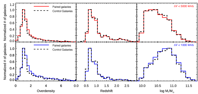
Figure 1: Normalized (at peak) distributions of environmental overdensity (left panel), spectroscopic redshift (middle panel), and stellar mass (right panel) of spectroscopic galaxy pairs (solid lines) (with projected separation $<150$ kpc, mass ratio $<4$, and spectroscopic redshift between 0.5 and 3 for the $\Delta V<5000$ km s^-1, top, and $\Delta V<1000$ km s^-1, bottom, samples, respectively) and their corresponding mass-, redshift-, and environment-matched control galaxies (dashed black lines).

We generate a control candidate sample of isolated galaxies that have no major or minor companion (within a mass ratio of 10) within a $\Delta z$ corresponding to a relative velocity of less than 5000 km s^-1, out to a projected separation of 150 kpc. We also update the control candidate sample by removing visually identified interacting or merging galaxies (Section 3.2) from this control candidate sample.

We construct the final control sample by using this updated control candidate sample. As we plan to control for the effects of redshift, stellar mass, and environment on the SFRs of galaxies, the distribution of these properties for the control sample should be similar to the distribution of these properties for the paired galaxy sample. Therefore, we find the control galaxies for a given paired galaxy by minimizing the difference between these properties of the paired galaxy and control candidate galaxies. Hence, for each paired galaxy, we select three control candidate galaxies with the smallest $(\Delta\log{M_{*}})^{2}+(\Delta z)^{2}+(1/40)(\Delta overdensity)^{2}$ from the updated control candidate sample. Here, 1/40 is a weighting factor for the environment overdensity. As the stellar mass, redshift, and overdensity spans quite different ranges of values and have a different distribution, to best match in all three dimensions and avoid overdensity-matching dominating, we used this weighting factor (1/40). For the final control sample, the controls match within a stellar mass of 0.15 dex, spectroscopic redshift within 0.15, and overdensity within a factor of one for more than 90% of the paired galaxies.

We show normalized distributions of the environmental overdensity, redshift, and stellar mass distribution of the final galaxy pair sample and corresponding control sample in Figure 1. The plots show that the environmental overdensity, redshift, and stellar mass distributions for the pair sample and its control sample are very similar to each other, i.e., the controls are well-matched to the pair sample, which is crucial for our analysis (see Shah et al., 2020). Our samples span a wide range of environment, redshift, and stellar mass. The distributions in Figure 1 show that the number of galaxy pairs in our sample decreases rapidly at high overdensities and high redshift.

4 Star formation Analysis

To estimate the star formation enhancement in merging and interacting galaxies, we first estimate the SFR of galaxies in the spectroscopic paired galaxy sample, visually identified interaction and merger galaxy samples, and the corresponding control galaxy samples as described in this section. We then compute the star formation enhancement and investigate how it varies with the galaxy pairs’ projected separation.

4.1 Measurement of SFR

We use the SED fitting tool Multi-wavelength Analysis of Galaxy Physical Properties (MAGPHYS; da Cunha et al., 2008) for fitting the model SEDs to the photometric data points (FUV-FIR band flux and flux-error values) to measure the SFR and stellar mass of galaxies. We choose MAGPHYS for the SED fitting process as it self-consistently fits observations from UV to FIR based on an energy balance argument. It considers a combination of hot and cold dust grains as well as PAHs to estimate attenuation. MAGPHYS uses the Bruzual & Charlot (2003) stellar population libraries. For estimating the SFR of the spectroscopic pairs and their corresponding control galaxies, we use their spectroscopic redshifts. For the visually identified interactions and merger galaxies and their corresponding control galaxies, we use their photometric redshifts.

The default version of MAGPHYS does not contain models with emission from an AGN component. However, it has been shown (e.g., Kirkpatrick et al., 2012) that a strong AGN can significantly impact the measured SFR of a galaxy, therefore, it is important to take such AGN activity into account. One way to identify galaxies that are strongly impacted by an AGN is to select galaxies that are poorly fit in the mid-infrared without the presence of an AGN component. Through substantial testing, it has been shown that the fitting residual at 8 $\mu$m can be indicative of strong AGN emission that dominates over star formation in the mid-infrared (Cooke et al., 2019). Therefore, for galaxies for which the $8\mu m$ residual percentile from the MAGPHYS fit ($100\times\frac{flux_{obs}-flux_{MAGPHYS}}{flux_{obs}}\%$) is more than $40\%$, we use a modified version of MAGPHYS called SED3FIT (Berta et al., 2013) that includes an AGN emission component to calculate their SFRs. We note that we elect not to fit the full sample using SED3FIT due to the computational time required and the fact that adding an additional component to the fit will often overestimate the importance of an AGN when there is not one present.

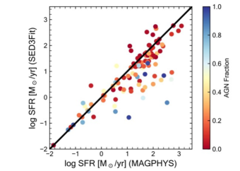
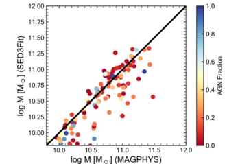
Figure 2: Comparison of the SFR (left) and stellar mass (right) measured using SED3FIT and MAGPHYS for galaxies in our sample with a large 8 $\mu$m residual suggesting the presence of an AGN component in the mid-IR. The color bar shows the value of the AGN fraction estimated using SED3FIT for a given galaxy.

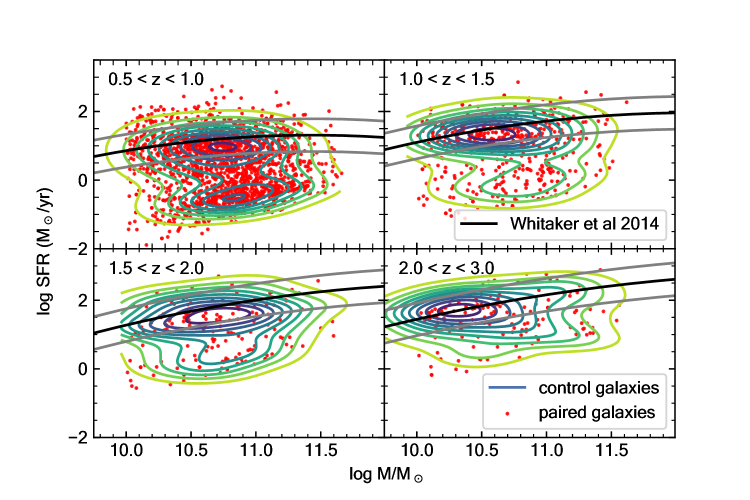
Figure 3: Distribution of paired galaxies (red scatter points) and controls (contours) on the SFR-M_∗ plane for (top to bottom) the $0.5<z<3.0$, $0.5<z<1.0$, $1.0<z<1.5$, $1.5<z<2.0$, and $2.0<z<3.0$ bins. The black solid line in each sub-plot corresponds to the star formation main sequence (Whitaker et al., 2014) in the given redshift range. The gray lines correspond to the SFR value above and below the SFMS by a factor of three in each redshift bin.

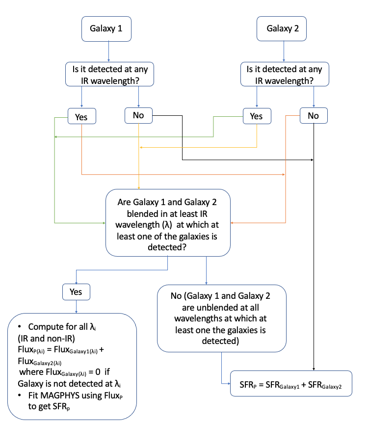
Figure 4: The decision tree for computing the combined SFR, SFR_P, of a galaxy pair, where galaxy1 and galaxy2 correspond to the primary and secondary galaxies in a given galaxy pair, respectively.

Figure 2 shows the comparison of the SFRs measured using SED3FIT and MAGPHYS. For most galaxies, the SFRs measured using the two SED fitting routines are similar to each other. However, for many galaxies the SFR measured with SED3FIT is lower than the value from MAGPHYS. This is mainly due to the fact that MAGPHYS can overestimate the total SFR when a strong AGN is present. Similarly, the right panel of Figure 2 shows a comparison between the stellar mass measured using SED3FIT and MAGPHYS for the same subset of galaxies with a large 8 $\mu$m residual. Again, for most galaxies, the stellar masses measured using SED3FIT are similar or lower than that from MAGPHYS. For these objects, we adopt the SED3FIT masses and SFRs in order to avoid overestimates due to the presence of a strong AGN. We note that these strong AGN are rare, and therefore, have minimal impact on our final results. For consistency, we remove any pairs from our sample that no longer satisfy the selection criteria as described in § 3 with these new stellar masses. This results in the removal of 17 pairs for the $\Delta V<1000$ km s^-1 sample and 22 pairs for the $\Delta V<5000$ km s^-1 sample. These removed pairs are reflected in the final pair sample presented in § 3 and the figures throughout the paper.

Using the results of our SED fits, we show the distribution of paired and control galaxies on the SFR-M_∗ plane in different redshift bins in Figure 3. We also show the corresponding star-forming main sequence (Whitaker et al., 2014) at each redshift. The two peaks in the contours in each plot correspond to the main sequence and the quiescent galaxy populations. Overall the control contours seem to trace the paired galaxy population well. The number of objects decreases rapidly with increasing redshift due to spectroscopic redshift incompleteness (especially at high redshifts). Note that the galaxy pair population spans a wide range of properties, including starbursts and quiescent galaxies, above and below the main sequence, respectively. The paired galaxies are required to have a minimum stellar mass of $10^{10}$ M_⊙, however the controls can have a slightly lower stellar mass than $10^{10}$ M_⊙ and so the contours extend slightly to the left of the paired galaxies in some of the sub-plots.

4.2 Blending of paired galaxies at IR wavelengths

The angular resolution of the images taken at 24 $\mu$m and longer wavelengths is poor relative to the optical/NIR filters and therefore, some galaxies in close pair systems are blended at MIR-FIR wavelengths. This means that for such pairs that are blended only at longer wavelength, the corresponding flux values will represent the pair and not the individual galaxies, which will affect their SFR measurement. Therefore, the flux values of the whole system, i.e., both galaxies combined, have to be used across all wavelengths when fitting an SED of the blended pair system in order to obtain an accurate measurement.

We compute the SFR of the whole galaxy pair system (both galaxies combined, SFR_P) for all galaxy pairs for a fair comparison with systems blended in the IR. Figure 4 illustrates the decision tree for measuring SFR_P for a given galaxy pair. We start with both galaxies (primary: galaxy1 and secondary: galaxy2) in the pair and determine if either of them are detected in any IR band. If neither of the two galaxies in a given galaxy pair are detected in any IR bands (black arrows), then the combined SFR_P is the summation of the SFR of the individual galaxies. If at least one of the galaxies in the pair is detected in at least one of the IR bands (say $\lambda$), then we check if the galaxies are blended at that wavelength $\lambda$. We repeat this process of checking blending for all wavelengths ($\lambda$1, $\lambda$2,…,$\lambda$n) in which at least one of the two galaxies are detected. If both galaxies are not blended at all wavelengths, we compute the SFR_P by adding the SFR of the two individual galaxies. If the two galaxies are blended in at least one of the wavelengths ($\lambda$ in $\lambda$1, $\lambda$2,…,$\lambda$n) then we combine the fluxes of the two galaxies at each wavelength to get the combined flux of the system in each band. We then fit the SED of this combined system using MAGPHYS to obtain SFR_P. If the $8\,\mu m$ percentile residual of the MAGPHYS fit for the combined system is more than 40 $\%$, then we refit the SED using SED3FIT to obtain the SFR_P. Only 115 galaxy pairs, i.e, $\sim 8.5\%$ of our total galaxy pair sample, are blended in the IR.

To facilitate a fair comparison between the pair system and their control counterparts, we compute the mean SFR of all controls of one of the two galaxies in a given pair ($\overline{SFR_{C1}}$) and repeat the process for the second galaxy ($\overline{SFR_{C2}}$). We then add these mean SFRs to obtain the final control SFR for a given galaxy pair ($SFR_{C}=\overline{SFR_{C1}}+\overline{SFR_{C2}}$). We propagate the errors in SFRs throughout this process to get the upper and lower error estimates for the SFR of combined control SFR ($SFR_{C}$) for a given galaxy pair. We repeat the process for all galaxy pairs.

5 SFR Enhancement

We define the SFR enhancement as the ratio of the weighted mean of the SFR of all galaxy pairs and the weighted mean SFR of all the corresponding combined controls, i.e.,

$$SFR\>Enhancement=\frac{\overline{SFR_{P}}}{\overline{SFR_{C}}}.$$ (1)

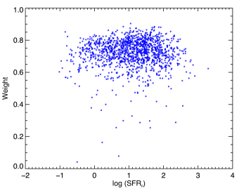
Figure 5: Distribution of weights (w_i) with respect to the SFR of galaxy pairs ($SFR_{P}$). The distribution shows that there is no significant trend between the weights and $SFR_{P}$.

For some galaxies, there are large errors on the SFR measured from our SED fits, which could be due to various reasons such as a poor fit, limitation of number of models in a given parameter space, large errors on the observed fluxes, etc. We consider this fact while estimating the average SFR of the pair sample ($SFR_{P}$) and the average SFR of the combined control sample (SFR_C). To decrease the dependence of the results on systems with large errors in the SFR measurement, we multiply the SFR_p and SFR_C values by a weighting function such that a lower weight value is assigned for a larger SFR percentile error and a higher weight value is assigned for a lower SFR percentile error. For a given galaxy pair, we use a weighting factor (w) based on the combined error (x) for SFR_P and $SFR_{C}$ using the formulae

$$x_{low}=\sqrt{\left(\frac{(\Delta SFR_{P})_{low}}{SFR_{P}}\right)^{2}+\left(\frac{(\Delta SFR_{C})_{low}}{SFR_{C}}\right)^{2}},$$ (2)

$$x_{up}=\sqrt{\left(\frac{(\Delta SFR_{P})_{up}}{SFR_{P}}\right)^{2}+\left(\frac{(\Delta SFR_{C})_{up}}{SFR_{C}}\right)^{2}},$$ (3)

$$x=\sqrt{\left(\frac{x_{low}^{2}+x_{up}^{2}}{2}\right)},$$ (4)

and

$$w=\frac{1}{1+x}.$$ (5)

Here, $(\Delta SFR_{P})_{low}$ and $(\Delta SFR_{P})_{up}$ are the lower and upper errors on the SFR of the given pair ($SFR_{P}$). Similary, $(\Delta SFR_{C})_{low}$ and $(\Delta SFR_{C})_{up}$ are the lower and upper errors on the SFR of the combined controls for a given galaxy pair ($SFR_{C}$). We also checked that our weights are not biased towards galaxy properties such as their M_∗ and SFR. Our enhancement values do not vary significantly if we use different weighting functions. For a given galaxy pair (for example, i), we compute the value of the combined error (x_i) using Eq. 2, 3, and 4. We then use the value of x_i to calculate the value of the weight (w_i) for the given galaxy pair using Eq. 5. The weighting function values (w_i) decrease with increasing average percentage error (x_i) on the SFR. We show the distribution of these weights (w_i) with respect to the SFR of galaxy pairs ($SFR_{P}$) in Figure 5. The figure shows that there is no significant trend between the SFR and the weights. Hence, by using the weights, our analysis is not biased towards higher or lower SFRs.

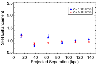
Figure 6: SFR enhancement as a function of projected separation of pairs. SFR enhancement is defined as the ratio of the weighted average of the SFR of the pair sample to that of the control sample (Equation 1). The filled blue circles and filled red diamonds correspond to the SFR enhancement for the $\Delta V<1000$ km s^-1 and $\Delta V<5000$ km s^-1 pair samples, respectively. The dotted line corresponds to a value of one, which represents no interaction-induced SFR enhancement. We see the highest level of SFR enhancement at a factor of 1.23${}^{+0.08}_{-0.09}$ ($\sim 2.6\sigma$) and 1.15${}^{+0.05}_{-0.04}$ ($\sim 3.0\sigma$) in the closest separation bin with projected pair separation $<$25 kpc for galaxy pair sample with $\Delta V<1000$ km s^-1 and $\Delta V<5000$ km s^-1, respectively. We note that there is a significant amount of scatter around the SFR enhancement value of one.

Finally, we compute the weighted average of the SFR for the galaxy pair sample and its corresponding control samples using

$$\overline{SFR_{P}}=\frac{\sum_{i}^{n_{p}}w_{i}(SFR_{P})_{i}}{\sum w_{i}}$$ (6)

and

$$\overline{SFR_{C}}=\frac{\sum_{i}^{n_{p}}w_{i}(SFR_{C})_{i}}{\sum w_{i}}.$$ (7)

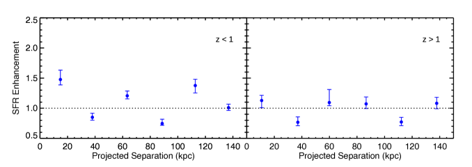
Figure 7: SFR enhancement as a function of projected separation for the galaxy pairs with $\Delta V<1000$ km s^-1 at $z<1$ (left) and $z>1$ (right). The dotted line corresponds to a value of one, which represents no interaction-induced SFR enhancement.

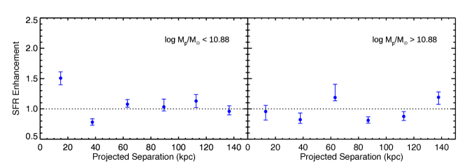
Figure 8: SFR enhancement as a function of projected separation for the galaxy pairs with $\Delta V<1000$ km s^-1 and with the stellar mass of the primary (more massive) galaxy $M_{p}$ less than 10.88 M_⊙ (left) and more than 10.88 M_⊙ (right) for the pair sample with $\Delta V<1000$ km s^-1. The dotted line corresponds to a value of one, which represents no interaction-induced SFR enhancement.

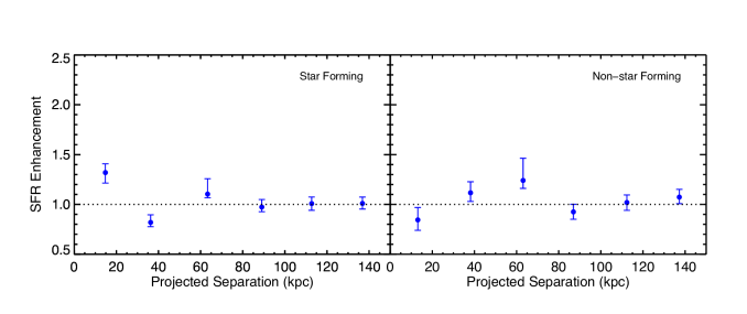
Figure 9: SFR enhancement as a function of projected separation for the pair sample with $\Delta V<1000$ km s^-1. The left and right hand side plots correspond to the results for star-forming blended pairs (and non-blended paired galaxies) and non-star forming blended pairs (and non-blended paired galaxies). The dotted line corresponds to a value of one, which represents no interaction-induced SFR enhancement.

We use the weighted average $\overline{SFR_{P}}$ and $\overline{SFR_{C}}$ values to estimate the SFR enhancement using Eq. 1. We divide the projected separation range ($0-150\thinspace$ kpc) into six different bins of width 25 kpc. We estimate the SFR enhancement in each bin. We show the SFR enhancement results for the spectroscopic galaxy pair samples with relative line of sight velocity $\Delta V<1000$ km s^-1 and $\Delta V<5000$ km s^-1 in Figure 6. We see the highest level of SFR enhancement of a factor of 1.23${}^{+0.08}_{-0.09}$ ($\sim 2.6\sigma$) and 1.15${}^{+0.05}_{-0.04}$ ($\sim 3.0\sigma$) in the closest separation bin of projected pair separation $<$25 kpc for the galaxy pair sample with $\Delta V<1000$ km s^-1 and $\Delta V<5000$ km s^-1, respectively. We note that there is significant scatter around the SFR enhancement value of one (a value indicating no enhancement). The results also do not show a clear trend of increasing SFR enhancement with decreasing projected separation. While the error bars on the SFR enhancements obtained using the weighted averages as described above are smaller than the ones calculated without weighting, the overall value of the SFR enhancement calculated with and without weights are very similar. We also note that we do not see a large difference between the $\Delta V<1000$ km s^-1 and $\Delta V<5000$ km s^-1 samples. Since there are more galaxies with $\Delta V<5000$ km s^-1, the error bars and resulting amount of scatter among the points are smaller. However, since pairs with $\Delta V<1000$ km s^-1 are more likely to be physically associated, we adopt this subsample for the remaining plots and discussion.

We then divide the $\Delta V<1000$ km s^-1 galaxy pair sample ($z_{median}\sim 1$) into two redshift bins ($z<1$ and $z>1$), with equal numbers of pairs in each bin, and calculate the SFR enhancement (Figure 7). We do not see a trend of increasing SFR enhancement with decreasing projected separations in either redshift bin. We see the highest enhancement of 1.48${}^{+0.16}_{-0.09}$ in the lowest projected separation bin ($<25$ kpc) at $z<1$. We see a large amount of scatter around the SFR enhancement value of one for both redshift bins. This scatter is most likely due to the sample size and does not represent a real trend in the SFR enhancement levels with separation.

Similarly, we also divide our $\Delta V<1000$ km s^-1 galaxy pair sample into two stellar mass bins separated at the median stellar mass ($10^{10.88}$ M_⊙) of the primary galaxy (more massive of the two galaxies) in a galaxy pair and represent the results in Figure 8. In the smallest projected separation bin, we see a SFR enhancement of 1.51${}^{+0.11}_{-0.10}$ ($\sim 4.6\sigma$) in the lower mass sample, which is $\sim 1.63\times$ higher (at $\sim 5.4\sigma$ level) than the SFR enhancement of 0.96${}^{+0.10}_{-0.14}$ in the same projected separation bin for the higher mass sample (log $M_{prim}/M_{\odot}>10.88$). Again, with this subdivided sample, we see a significant amount of scatter around the SFR enhancement value of one.

Furthermore, we divide the $\Delta V<1000$ km s^-1 galaxy pair sample into star-forming (SF) paired galaxies and non-star forming (non-SF/quiescent) paired galaxies identified based on whether SFR of the galaxy is higher or lower than the specific SFR of $sSFR=(1+z)^{2.5}\times 10^{-11}$ (Speagle et al., 2014), respectively. In the case of blended pairs, we apply this criterion to the sSFR of the whole blended system. We also select new sets of SF (non-SF) controls for this SF (non-SF) blended pairs and non-blended paired galaxies using the same method described previously. We show the SFR enhancement results in Figure 9. In the closest separation bin, we see a SFR enhancement of 1.32${}^{+0.09}_{-0.11}$ in the SF sample, which is $\sim 1.57\times$ larger than for the non-SF sample (0.84${}^{+0.12}_{-0.10}$). Here also, the results show a significant amount of scatter around the SFR enhancement value of one. We also compare the SFR enhancements in our primary galaxy sample to the secondary galaxy sample of the non-blended galaxy pairs. We do not see a significant difference in SFR enhancement of these two samples (not shown here).

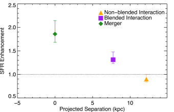
Figure 10: SFR enhancement for our visually identified mergers (filled green diamonds), blended interactions (filled purple squares), and non-blended interactions (filled orange triangles) as a function of their median projected separations. The merged/coalesced systems are plotted at a separation of zero, since they are no longer in a pair but are in a single coalesced galaxy. The dotted line corresponds to a value of one, which represents no interaction-induced SFR enhancement. Note that for this sample, we see a clear trend of increasing SFR enhancement with decreasing projected separation, with the largest level of enhancement seen in the coalesced systems.

We present the SFR enhancement for our visually identified interactions and merger samples in Figure 10. We see enhancements of 1.86${}^{+0.29}_{-0.18}$, 1.31${}^{+0.16}_{-0.08}$, and 0.90${}^{+0.10}_{-0.06}$ for our visually identified merger sample, blended-interaction sample, and non-blended interaction sample, respectively. For this sample, we see a clear trend of increasing SFR enhancement for decreasing median projected separation, with the largest enhancement seen for coalesced merger systems.

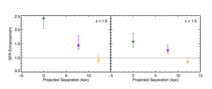
Figure 11: SFR enhancement for our visually identified mergers (filled green diamonds), blended interactions (filled purple squares), and non-blended interactions (filled orange triangles) at $z<1.6$ (left) and $z<1.6$ (right) compared to their star-forming control samples. The dotted line corresponds to a value of one, which represents no interaction-induced SFR enhancement. While we see evidence of increasing enhancement with decreasing projected separation in both redshift bins, we see a decreased level of enhancement for the $z>1.6$ bin.

Since we use photometric redshift for the visually identified sample, rather than spectroscopic redshifts as for the galaxy pair sample, the median redshift of these galaxies is higher than that of the pair sample. We divide our visually identified interaction and merger samples into two redshift bins separated at the median redshift $z_{median}\sim 1.6$ of the samples. We show these results in Figure 11. At low $z$ ($0.5<z<1.6$), we find that the SFR enhancement levels are a factor of 2.40${}^{+0.62}_{-0.37}$, 1.44${}^{+0.35}_{-0.12}$, and 0.93${}^{+0.20}_{-0.11}$ for our merger, blended, and non-blended interaction samples, respectively. Similarly, at high $z$ ($z>1.6$), we see enhancement values of 1.58${}^{+0.29}_{-0.20}$, 1.27${}^{+0.19}_{-0.10}$, and 0.88${}^{+0.11}_{-0.08}$ for our merger, blended, and non-blended interaction samples, respectively. In both redshift bins, we find that there is a clear trend of increasing SFR enhancement with decreasing projected separation with the largest enhancement see for the coalesced merger systems. We also find that the level of enhancement at $z<1.6$ is a factor of $\sim 1.5$ higher than the enhancement at $z>1.6$, suggesting that there is an evolution in the interaction-induced SFR enhancement between these two bins.

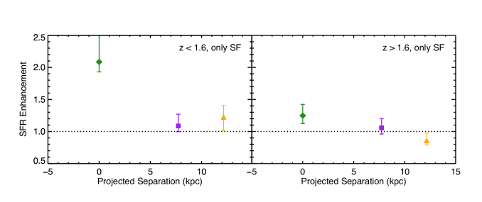
Figure 12: SFR enhancement for only star-forming visually identified mergers (filled green diamonds), blended interactions (filled purple squares), and non-blended interactions (filled orange triangles) at $z<1.6$ (left) and $z<1.6$ (right) compared to their star-forming control samples.

Finally, we select the subset of galaxies in the visually identified sample that are star-forming using the same criteria as for the pair sample ($sSFR>(1+z)^{2.5}\times 10^{-11}$; Speagle et al. 2014) and selected their corresponding star-forming control samples. As shown in Figure 12, we calculate a SFR enhancement of 2.08${}^{+0.42}_{-0.15}$, 1.09${}^{+0.18}_{-0.09}$, and 1.23${}^{+0.18}_{-0.21}$ at low $z$ for our merger, blended, and non-blended interaction samples, respectively. At high z, the corresponding SFR enhancement values are 1.23${}^{+0.18}_{-0.12}$, 1.06${}^{+0.15}_{-0.10}$, and 0.86${}^{+0.11}_{-0.07}$. We find that for the coalesced systems, the SFR enhancement if a factor of $\sim 1.7$ times higher at $z<1.6$ than at $z>1.6$.

6 Discussion

We investigate the level of SFR enhancement in major spectroscopic galaxy pairs relative to their stellar mass-, redshift-, and environment-matched control sample of isolated galaxies at $0.5<z<3.0$. We find that there is a slight SFR enhancement of a factor of 1.23${}^{+0.08}_{-0.09}$ ($\sim 2.6\sigma$) and 1.15${}^{+0.05}_{-0.04}$ ($\sim 3.0\sigma$) in the lowest projected separation bin ($<25$ kpc) for our $\Delta V<1000$ km s^-1 and $\Delta V<5000$ km s^-1 spectroscopic galaxy pair samples, respectively. We find a stronger level of enhancement of a factor of 1.86${}^{+0.29}_{-0.18}$ in the coalesced visually identified mergers. We compare these result with similar studies in the literature.

6.1 Comparison with Studies in the Local Universe

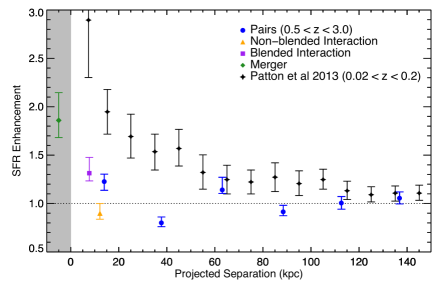
Figure 13: Comparison of the SFR enhancement as a function of the projected separation of interactions and mergers ($0.5<z<3.0$) to the pair sample in the local universe ($0.02<z<0.20$) from Patton et al. (2013). SFR enhancement is defined as the ratio of the average SFR of the pair sample to that of the control sample (Equation 1.) The dotted line corresponds to a value of one, which represents no interaction-induced SFR enhancement. The blue filled circles show the SFR enhancement for our complete galaxy pair sample ($log(M_{pair}/M_{\odot})>10.3$ and $0.5<z<3.0$). The filled green diamond, filled purple square, and filled orange triangle correspond to the SFR enhancements for our visually identified merger sample, blended interaction sample, and non-blended interaction sample, respectively. The gray region corresponds to the merger (or post merger) stage. The filled black stars correspond to the Patton et al. (2013) SFR enhancement results for a pair sample in the local ($0.02<z<0.20$) universe selected from SDSS observations. While we see significant enhancement for galaxy mergers in our high redshift sample, the overall level of enhancement is less than that seen in the local pair sample, indicative of a change in role of interactions and mergers in inducing star formation over cosmic time.

In contrast to our results at $0.5<z<3.0$, there are several studies in the local universe ($z\sim 0$) that find considerable SFR enhancement in galaxy interactions by comparing the star formation of interacting and isolated (control) galaxies (e.g., Alonso et al. (2004); Woods & Geller (2007); Ellison et al. (2008); Xu et al. (2010); Ellison et al. (2013b); Patton et al. (2013)). Almost all of these studies find the strongest enhancement for pairs with projected separation less than 30 kpc.

The closest study on SFR enhancement in the local universe to our high redshift study is Patton et al. (2013) (P13 from here on). Therefore, we compare our SFR enhancement results with P13 results to understand how the level of SFR enhancement differs at high redshift compared to the local universe. P13 measure the SFR enhancement for local pairs ($0.02<z<0.2$ and stellar mass ratio $<10$) identified using SDSS observations. We compare their SFR enhancement results with our results in Figure 13. The highest level of SFR enhancement that they find is a factor of $\sim 2.9$ for pairs with projected separation less than 10 kpc. Their estimated SFR enhancement value for pairs with projected separation between 10 kpc and 20 kpc is $\sim 1.95$, which is a factor of 1.6 times ($\sim 3.2\sigma$) higher than our SFR enhancement result of 1.23${}^{+0.08}_{-0.09}$ for pairs with projected separation between 0 kpc and 25 kpc (median $\sim 14$ kpc). P13 see a clear trend of increasing SFR enhancement with decreasing projected separation. We find that this trend is absent in our for pairs with projected separations of $>$25 kpc based on Figure 13, at separations $<$25 kpc, we see an overall trend of increasing SFR enhancement with decreasing projected separation. This is particulary notable for our visually identified merger and interaction sample. For the SFR enhancement our blended interactions sample, we see a value slightly less than one, which could be due to low number statistics. Unlike our results, P13 observe an enhancement in SFR for pairs with projected separations of up to 150 kpc. Many factors can impact the measurement of SFR enhancement (such as redshift evolution, sample selection, SFR measurement method, etc.) that would be cumulatively responsible for the differences between our results and P13 results.

Apart from the clear differences in the redshift range of our pair sample ($0.5<z<3.0$) and their pair sample ($0.02<z<0.2$), the P13 pair sample also consists of both major and minor pairs (mass ratio $<10$), unlike our sample of only major galaxy pairs. They also apply a stricter line of sight velocity difference constraint to identify galaxy pairs ($\Delta V<300$ km s^-1) compared to our relatively liberal constraint ($\Delta V<1000$ km s^-1). Furthermore, similar to many local studies, P13 select only star forming galaxies identified using emission lines, which means that their sample consists of only star-forming galaxies compared to our sample which also contains non-star forming galaxies. If we only consider the subset of our galaxies that are star-forming, our SFR enhancement result (Figure 9) of 1.32${}^{+0.09}_{-0.11}$ at 0-25 kpc is 1.5$\times$ (compared to 1.6$\times$ for the complete sample), lower than P13 SFR enhancement at 10-20 kpc. Hence, even for the star-forming sample, our pair sample ($0.5<z<3.0$) shows less SFR enhancement than a local ($0.02<z<2.0$) pair sample P13 at similar projected separations.

Similarly, Ellison et al. (2013a) find a SFR enhancement of $\sim 3.5$ in a post-merger sample compared to the controls generated using SDSS observations. Their SFR enhancement is $\sim 1.9\times$ higher than our visually identified merger sample ($0.5<z<3.0$). For our sample divided into two redshift bins, the local enhancement for coalesced mergers is $1.4\times$ and $2.2\times$ higher than our $0.5<z<1.6$ and $1.6<z<3.0$ samples, respectively. This suggest evolution in the merger-induced star formation enhancement between these three redshift bins.

6.2 Comparison with Simulations

A relative decrease in the SFR enhancement level and its duration in merging galaxies with a significantly higher gas fraction has been suggested by some studies conducted using idealized binary merger simulations (Bournaud et al., 2011; Hopkins et al., 2013; Scudder et al., 2015; Fensch et al., 2017). For example, Fensch et al. (2017) use idealized binary merger simulations to study the effect of a galaxy merger on the SFR of galaxies and show that the amount and the duration of the merger-induced star formation excess is about ten times lower for a high redshift galaxy (gas fraction $\sim$ 60%, $z\sim 2$) mergers compared to their low redshift counterparts (gas fraction $\sim 10\%$, $z\sim 0$). Fensch et al. (2017) suggest that the high turbulence in these systems makes further compression of gas and generation and propagation of inflows weaker at high-$z$ than in low-$z$ interactions, causing a considerable decrease in the ability of mergers to increase the SFR of galaxies at high-$z$.

Similarly, using a suite of nine binary merger simulations with the same orbital parameters but with varying gas fractions ($0.04\leq M_{*}/M_{gas}\leq 1.78$), Scudder et al. (2015) find an anti-correlation between the SFR enhancement at coalescence and the pre-merger gas fraction of galaxies. However, such studies based on binary merger simulations usually do not contain cosmic gas inflows and have a very limited sample size. Therefore, we also compare our results with SFR enhancement studies based on hydrodynamical cosmological simulations. Many of these studies also show the weakening of enhancement levels with increasing redshift. For example, Patton et al. (2020) present a study (similar to their observational study P13) of interacting galaxy pairs identified in the IllustrisTNG cosmological simulations. They select massive ($M_{*}>10^{10}M_{\odot}$) galaxy pairs at $0\leq z<1$ and their corresponding stellar mass-, redshift-, and environment-matched controls and see a gradual decrease in the sSFR enhancement levels with increasing redshift in the same projected separation bin.

Martin et al. (2017) also find a decrease in merger-induced SFR enhancement level with increasing redshift in the Horizon-AGN cosmological simulations. This reduction in SFR enhancement is also suggested by our higher SFR enhancement result (2.40${}^{+0.62}_{-0.37}$) for the visually identified merger sample at low $z$ ($0.5<z<1.6$) compared to a lower SFR enhancement (1.58${}^{+0.29}_{-0.20}$) at high $z$ ($1.6<z<3.0$) shown Figure 11. Comparisons of our results with the local results, as discussed earlier, also show this reduction in SFR enhancement with redshift.

Hani et al. (2020) also use IllustrisTNG (TNG300-1) to identify post-mergers at $0\leq z\leq 1$ and a well-matched control sample. They see a SFR enhancement of a factor of $\sim 2$ in their merger sample compared to the control sample, which is within error bars of our SFR enhancement result (2.40${}^{+0.62}_{-0.37}$) for the visually identified merger sample at $z<1.6$ (left panel of Figure 11). They match SF mergers with SF controls, which is analogous to our results for SF mergers (Figure 12), where our SFR enhancement (2.08${}^{+0.42}_{-0.15}$) for the merger sample at low $z$ ($0.5<z<1.6$) is almost same as their SFR enhancement ($\sim 2$).

While Hani et al. (2020) see no redshift evolution in their SF mergers compared to SF controls over $0\leq z<1$, we see a $1.75\times$ higher SFR enhancement at low-$z$ ($z<1.6$) compared to high-$z$ ($z>1.6$). Hence, the comparison suggests that there might be a mild evolution of SFR enhancement with redshift, which becomes detectable when enhancement is compared over a larger redshift range ($0.5<z<3.0$ in our study), and which could be missed when enhancement is compared over a smaller redshift range ($0\leq z\leq 1$ in Hani et al., 2020). For a larger redshift range, our SFR enhancement value (1.86${}^{+0.29}_{-0.18}$) for the visually identified merger sample at $0.5<z<3.0$ is within the error bars of the sSFR enhancement in a merger sample compared to a mass-matched control sample at $0<z<2.5$ in the Simba Simulation (Rodríguez Montero et al., 2019).

6.3 Comparison with Previous High Redshift Studies

There are also observational studies exploring the effects of interactions and mergers on the SFR of galaxies at high redshift. For example, Lackner et al. (2014) identify merging galaxies in the COSMOS field at $0.25<z<1.00$ with log $M_{*}/M_{\odot}>10.6$ by applying an automated method of median-filtering the high-resolution COSMOS HST images to distinguish two concentrated galaxy nuclei at small separations (2.2-8 kpc). This method is sensitive to very close pairs and advanced stage mergers with double nuclei and hence are all roughly at a similar merger stage. We note that because of the differences in the selection criteria, some objects in their sample could be included in our visually identified merger and blended interaction samples. They find a SFR enhancement of value of 2.1$\pm$0.6 in their merging sample compared to the non-merging sample. Their result is consistent with our result for the visually identified merger sample (2.40${}^{+0.62}_{-0.37}$) and blended-interaction sample (1.44${}^{+0.35}_{-0.12}$) at $0.5<z<1.6$ (left panel of Figure 11). This comparison also shows the importance of comparing the definition or identification criteria (e.g., merging galaxies in this case) when comparing the results of two studies. Our SFR enhancement result for the visually identified merger sample at $z>1.6$ is also consistent with the sSFR enhancement ($\sim 2.2$) in mergers compared to non-interacting galaxies at ($z\sim 2$) found in Kaviraj et al. (2013).

In contrast to these results, Wilson et al. (2019) do not see a significant SFR enhancement in merging galaxy pairs compared to a control sample of isolated galaxies at $1.5\lesssim z\lesssim 3.5$. The differences in our results could be due to differences in the pair selection and control matching criteria used. They identify pairs as two objects whose spectra were obtained on the same Keck/MOSFIRE slit. Their 30 galaxy pairs have projected separations less than 60 kpc, relative velocities less than 500 km s^-1, and stellar mass ratios ranging from 1.1 to 550 ($<3$ for 40 $\%$ of pairs). These criteria mean that their sample consists of major interactions (mass ratio $<4$), minor interactions (mass ratio between 4 and 10), and systems with even larger mass ratios; hence, a much larger difference between the stellar mass of the primary and secondary galaxies, which can significantly dilute the estimated interaction effects.

Similarly, Pearson et al. (2019) train and use convolutional neural networks to identify over 200,000 galaxies at $0.0<z<4.0$ in the SDSS, KiDS, and CANDELS surveys as merging or non-merging galaxies. They then compare the SFR of merging and non-merging galaxies and find a slight enhancement of $\sim 1.2$ in merging galaxies compared to their non-merging sample. Our SFR enhancement results for pairs in the closest projected separation bin as well the blended-interactions in strong agreement with their SFR enhancement results. However, we also note a large difference in the redshift range and other selection criteria, making a direct comparison difficult.

6.4 Variation in SFR Enhancement with Stellar Mass

Some studies also find a decrease in the SFR enhancement or sSFR enhancement with the stellar mass of galaxies. For example, Hani et al. (2020) find a change in sSFR enhancement with stellar mass. For $M_{*}<10^{11}M_{\odot}$ they see an sSFR enhancement of 1.5-2.5 (depending on the TNG simulation used), which reduces to $\sim 1$ at higher masses. The same trend is also seen for mergers in the Simba Simulation (Rodríguez Montero et al., 2019). A similar trend of decreasing level of SFR enhancement with increasing stellar mass is also seen in the merger sample of Silva et al. (2018). Our SFR enhancement results for galaxy pairs with $M_{*}<10^{10.88}M_{\odot}$ (1.51${}^{+0.11}_{-0.10}$) and $M_{*}>10^{10.88}M_{\odot}$ (0.96${}^{+0.10}_{-0.14}$) shown in Figure 8 suggest a similar trend as seen in the above-mentioned studies.

As discussed in Shah et al. (2020), selecting a well-matched control sample is crucial for this type of analysis. While we have only selected isolated galaxies that do not show obvious visual signs of interactions or mergers as control candidates, our control sample can unintentionally still contain merging galaxies that were not identified as mergers in the visually identified sample. This is mainly due to the difficulty in identifying mergers and interactions at high redshift due to weak or non-detectable merger signatures. This potential contamination of mergers or interactions in the control sample would dilute the estimated SFR enhancement in our sample. Hence, the estimated SFR enhancement values are most likely lower limits of the actual SFR enhancements.

7 Summary

The goal of this study is to understand the effect of galaxy interactions and mergers on the star formation of galaxies at high redshift and compare the SFR enhancement results with the local interaction results in order to understand evolutionary effects on the role of interactions in driving star formation activity. We used our sample of major spectroscopic galaxy pairs, visually identified interactions and mergers, and their corresponding control samples at $0.5<z<3.0$, as described in detail in Shah et al. (2020). The samples were generated using deep multi-wavelength photometric and spectroscopic observations from the CANDELS and COSMOS surveys. Our 1327 (2351) spectroscopic galaxy pairs satisfy five criteria: a spectroscopic redshift in the range $0<z<3$, a relative line of sight velocity less than 1000 (5000)  km s^-1, stellar mass of each of the galaxies in a pair more than 10${}^{10}M_{\odot}$, stellar mass ratio of the primary (more massive) to the secondary galaxy less than four, and projected separation less than 150 kpc. Our controls are closely matched to individual paired galaxies in their stellar mass, redshift, and environment density. We estimate the SFR enhancement in the galaxy pair sample by taking the ratio of the weighted mean of the SFR of the galaxy pair sample over that of the corresponding control sample. Our main findings are:

1. We see evidence for a slight enhancement of a factor 1.23${}^{+0.08}_{-0.09}$ ($\sim 2.6\sigma$) in the closest projected separation bin ($d<25$ kpc) for our full galaxy pair sample (Figure 6). However, we also see a significant amount of scatter around the SFR enhancement value of one at all separation bins. Therefore, in contrast to results for local pair studies, we do not see a clear trend of increasing SFR enhancement with decreasing projected separation in our spectroscopic galaxy pair sample.

2. We divide our pair sample by redshift and find that at the closes separation ($<25\thinspace kpc$), the low-$z$ ($0.5<z<1$ sample has a higher SFR enhancement than the high-$z$ ($1<z<3.0$) sample by a factor of $\sim 1.3$ (2.2$\sigma$) (Figure 7). Though this difference is marginally significant, it is consistent with interaction-induced star formation having a decreased role at higher redshift.

3. We see an enhancement level of a factor of 1.86${}^{+0.29}_{-0.18}$ ($\sim 3\sigma$) in our visually identified merger sample. There is a clear trend of increasing SFR enhancement with decreasing projected separation in our visually identified sample of interactions and mergers as shown in Figure 10. The sample shows this trend at both low-$z$ ($0.5<z<1.6$) and high-$z$ ($1.6<z<3.0$) (2.40${}^{+0.62}_{-0.37}$ vs. 1.58${}^{+0.29}_{-0.20}$; Figure 11), with the level of enhancement decreasing with increasing redshift. This result again suggests evolution in the level of merger-driven star formation with time.

4. We see an enhancement of 1.51${}^{+0.11}_{-0.10}$ ($\sim 4.6\sigma$) for our pairs with a lower mass primary galaxy ($M_{prim}<10.88\,M_{\odot}$) compared to the enhancement (0.96${}^{+0.10}_{-0.14}$) in pairs with a higher mass primary galaxy ($M_{prim}>10.88\,M_{\odot}$) in the same closest projected separation bin. This factor of 1.6 difference in the enhancement level hints at stronger effects of interactions in enhancing SF of lower mass galaxy pairs. This is consistent with the results of both observational (e.g., Silva et al., 2018) and simulation (e.g., Rodríguez Montero et al., 2019) studies.

5. We also see a slightly higher level of SFR enhancement (1.32${}^{+0.09}_{-0.11}$ vs. 0.84${}^{+0.12}_{-0.10}$) in the star-forming paired galaxy sample compared to the non-star forming paired galaxy sample in the closest projected separation bin. For blended pairs, we used the combined SFR of the system to check if it is star-forming or non-star forming.

Overall, our results show a slight SFR enhancement in close pairs and a significant enhancement in advanced stage mergers at $0.5<z<3.0$, and an absence of SFR enhancement at larger pair separations ($>25$ kpc). Comparison of our results with local studies (Figure 13) suggests that the effect of interactions and mergers on SFR weakens at high $z$, which is consistent with the predictions of some simulations. Our study on SFR enhancement in a large sample of spectroscopic galaxy pairs and mergers provides a deeper understanding of the role of galaxy mergers and interactions in galaxy evolution in the high redshift universe. Future spectroscopic surveys of close pairs at high redshift are required, especially at $z>2$, to increase the sample size and improve statistics to enable a more comprehensive analysis of the evolving role of galaxy interactions over cosmic time.

References

- Alonso et al. (2004) Alonso, M. S., Tissera, P. B., Coldwell, G., & Lambas, D. G. 2004, MNRAS, 352, 1081
- Arnouts et al. (2002) Arnouts, S., Moscardini, L., Vanzella, E., et al. 2002, MNRAS, 329, 355
- Arnouts et al. (2013) Arnouts, S., Le Floc’h, E., Chevallard, J., et al. 2013, A&A, 558, A67
- Ashby et al. (2013) Ashby, M. L. N., Willner, S. P., Fazio, G. G., et al. 2013, ApJ, 769, 80
- Ashby et al. (2015) —. 2015, ApJS, 218, 33
- Balestra et al. (2010) Balestra, I., Mainieri, V., Popesso, P., et al. 2010, A&A, 512, A12
- Barger et al. (2008) Barger, A. J., Cowie, L. L., & Wang, W.-H. 2008, ApJ, 689, 687
- Barmby et al. (2008) Barmby, P., Huang, J.-S., Ashby, M. L. N., et al. 2008, ApJS, 177, 431
- Barnes (2004) Barnes, J. E. 2004, MNRAS, 350, 798
- Barrera-Ballesteros et al. (2015) Barrera-Ballesteros, J. K., Sánchez, S. F., García-Lorenzo, B., et al. 2015, A&A, 579, A45
- Barro et al. (2019) Barro, G., Pérez-González, P. G., Cava, A., et al. 2019, ApJS, 243, 22
- Bergvall et al. (2003) Bergvall, N., Laurikainen, E., & Aalto, S. 2003, A&A, 405, 31
- Berta et al. (2013) Berta, S., Lutz, D., Santini, P., et al. 2013, A&A, 551, A100
- Bertin & Arnouts (1996) Bertin, E., & Arnouts, S. 1996, A&AS, 117, 393
- Blumenthal et al. (2020) Blumenthal, K. A., Moreno, J., Barnes, J. E., et al. 2020, MNRAS, 492, 2075
- Bournaud et al. (2011) Bournaud, F., Chapon, D., Teyssier, R., et al. 2011, ApJ, 730, 4
- Bradshaw et al. (2013) Bradshaw, E. J., Almaini, O., Hartley, W. G., et al. 2013, MNRAS, 433, 194
- Brinchmann et al. (2004) Brinchmann, J., Charlot, S., White, S. D. M., et al. 2004, MNRAS, 351, 1151
- Bruzual & Charlot (2003) Bruzual, G., & Charlot, S. 2003, MNRAS, 344, 1000
- Calzetti et al. (2000) Calzetti, D., Armus, L., Bohlin, R. C., et al. 2000, ApJ, 533, 682
- Capak et al. (2004) Capak, P., Cowie, L. L., Hu, E. M., et al. 2004, AJ, 127, 180
- Chabrier (2003) Chabrier, G. 2003, PASP, 115, 763
- Coil et al. (2004) Coil, A. L., Davis, M., Madgwick, D. S., et al. 2004, ApJ, 609, 525
- Coil et al. (2011) Coil, A. L., Blanton, M. R., Burles, S. M., et al. 2011, ApJ, 741, 8
- Comparat et al. (2015) Comparat, J., Richard, J., Kneib, J.-P., et al. 2015, A&A, 575, A40
- Cooke et al. (2019) Cooke, K. C., Kartaltepe, J. S., Tyler, K. D., et al. 2019, ApJ, 881, 150
- Cooper et al. (2011) Cooper, M. C., Aird, J. A., Coil, A. L., et al. 2011, ApJS, 193, 14
- Cooper et al. (2012a) Cooper, M. C., Yan, R., Dickinson, M., et al. 2012a, MNRAS, 425, 2116
- Cooper et al. (2012b) Cooper, M. C., Griffith, R. L., Newman, J. A., et al. 2012b, MNRAS, 419, 3018
- Cowie et al. (2004) Cowie, L. L., Barger, A. J., Hu, E. M., Capak, P., & Songaila, A. 2004, AJ, 127, 3137
- Croom et al. (2001) Croom, S. M., Warren, S. J., & Glazebrook, K. 2001, MNRAS, 328, 150
- da Cunha et al. (2008) da Cunha, E., Charlot, S., & Elbaz, D. 2008, MNRAS, 388, 1595
- Daddi et al. (2004) Daddi, E., Cimatti, A., Renzini, A., et al. 2004, ApJ, 600, L127
- Daddi et al. (2010) Daddi, E., Elbaz, D., Walter, F., et al. 2010, ApJ, 714, L118
- Dahlen et al. (2013) Dahlen, T., Mobasher, B., Faber, S. M., et al. 2013, ApJ, 775, 93
- Damjanov et al. (2018) Damjanov, I., Zahid, H. J., Geller, M. J., Fabricant, D. G., & Hwang, H. S. 2018, ApJS, 234, 21
- Darg et al. (2010) Darg, D. W., Kaviraj, S., Lintott, C. J., et al. 2010, MNRAS, 401, 1552
- Darvish et al. (2015) Darvish, B., Mobasher, B., Sobral, D., Scoville, N., & Aragon-Calvo, M. 2015, ApJ, 805, 121
- Davis et al. (2007) Davis, M., Guhathakurta, P., Konidaris, N. P., et al. 2007, ApJ, 660, L1
- Di Matteo et al. (2008) Di Matteo, P., Bournaud, F., Martig, M., et al. 2008, A&A, 492, 31
- Dickinson et al. (2003) Dickinson, M., Giavalisco, M., & GOODS Team. 2003, in The Mass of Galaxies at Low and High Redshift, ed. R. Bender & A. Renzini, 324
- Donzelli & Pastoriza (1997) Donzelli, C. J., & Pastoriza, M. G. 1997, ApJS, 111, 181
- Duncan et al. (2019) Duncan, K., Conselice, C. J., Mundy, C., et al. 2019, ApJ, 876, 110
- Elbaz et al. (2007) Elbaz, D., Daddi, E., Le Borgne, D., et al. 2007, A&A, 468, 33
- Ellison et al. (2013a) Ellison, S. L., Mendel, J. T., Patton, D. R., & Scudder, J. M. 2013a, MNRAS, 435, 3627
- Ellison et al. (2013b) Ellison, S. L., Mendel, J. T., Scudder, J. M., Patton, D. R., & Palmer, M. J. D. 2013b, MNRAS, 430, 3128
- Ellison et al. (2008) Ellison, S. L., Patton, D. R., Simard, L., & McConnachie, A. W. 2008, AJ, 135, 1877
- Fensch et al. (2017) Fensch, J., Renaud, F., Bournaud, F., et al. 2017, MNRAS, 465, 1934
- Ferreras et al. (2009) Ferreras, I., Pasquali, A., Malhotra, S., et al. 2009, ApJ, 706, 158
- Galametz et al. (2013) Galametz, A., Grazian, A., Fontana, A., et al. 2013, ApJS, 206, 10
- Giavalisco et al. (2004) Giavalisco, M., Ferguson, H. C., Koekemoer, A. M., et al. 2004, ApJ, 600, L93
- Grogin et al. (2011) Grogin, N. A., Kocevski, D. D., Faber, S. M., et al. 2011, ApJS, 197, 35
- Guo et al. (2013) Guo, Y., Ferguson, H. C., Giavalisco, M., et al. 2013, ApJS, 207, 24
- Hani et al. (2020) Hani, M. H., Gosain, H., Ellison, S. L., Patton, D. R., & Torrey, P. 2020, MNRAS, 493, 3716
- Hasinger et al. (2018) Hasinger, G., Capak, P., Salvato, M., et al. 2018, ApJ, 858, 77
- Hopkins et al. (2013) Hopkins, P. F., Cox, T. J., Hernquist, L., et al. 2013, MNRAS, 430, 1901
- Hopkins et al. (2008) Hopkins, P. F., Hernquist, L., Cox, T. J., & Kereš, D. 2008, ApJS, 175, 356
- Ilbert et al. (2006) Ilbert, O., Arnouts, S., McCracken, H. J., et al. 2006, A&A, 457, 841
- Ilbert et al. (2009) Ilbert, O., Capak, P., Salvato, M., et al. 2009, ApJ, 690, 1236
- Inami et al. (2017) Inami, H., Bacon, R., Brinchmann, J., et al. 2017, A&A, 608, A2
- Kartaltepe et al. (2010) Kartaltepe, J. S., Sanders, D. B., Le Floc’h, E., et al. 2010, ApJ, 721, 98
- Kartaltepe et al. (2015a) Kartaltepe, J. S., Mozena, M., Kocevski, D., et al. 2015a, ApJS, 221, 11
- Kartaltepe et al. (2015b) Kartaltepe, J. S., Sanders, D. B., Silverman, J. D., et al. 2015b, ApJ, 806, L35
- Kaviraj et al. (2013) Kaviraj, S., Cohen, S., Windhorst, R. A., et al. 2013, MNRAS, 429, L40
- Kirkpatrick et al. (2012) Kirkpatrick, A., Pope, A., Alexander, D. M., et al. 2012, ApJ, 759, 139
- Knapen & James (2009) Knapen, J. H., & James, P. A. 2009, ApJ, 698, 1437
- Koekemoer et al. (2011) Koekemoer, A. M., Faber, S. M., Ferguson, H. C., et al. 2011, ApJS, 197, 36
- Kriek et al. (2015) Kriek, M., Shapley, A. E., Reddy, N. A., et al. 2015, ApJS, 218, 15
- Krogager et al. (2014) Krogager, J.-K., Zirm, A. W., Toft, S., Man, A., & Brammer, G. 2014, ApJ, 797, 17
- Kurk et al. (2013) Kurk, J., Cimatti, A., Daddi, E., et al. 2013, A&A, 549, A63
- Lackner et al. (2014) Lackner, C. N., Silverman, J. D., Salvato, M., et al. 2014, AJ, 148, 137
- Laidler et al. (2007) Laidler, V. G., Papovich, C., Grogin, N. A., et al. 2007, PASP, 119, 1325
- Laigle et al. (2016) Laigle, C., McCracken, H. J., Ilbert, O., et al. 2016, ApJS, 224, 24
- Lambas et al. (2003) Lambas, D. G., Tissera, P. B., Alonso, M. S., & Coldwell, G. 2003, MNRAS, 346, 1189
- Larson & Tinsley (1978) Larson, R. B., & Tinsley, B. M. 1978, ApJ, 219, 46
- Lawrence et al. (2007) Lawrence, A., Warren, S. J., Almaini, O., et al. 2007, MNRAS, 379, 1599
- Le Fèvre et al. (2004) Le Fèvre, O., Vettolani, G., Paltani, S., et al. 2004, A&A, 428, 1043
- Le Fèvre et al. (2013) Le Fèvre, O., Cassata, P., Cucciati, O., et al. 2013, A&A, 559, A14
- Le Fèvre et al. (2015) Le Fèvre, O., Tasca, L. A. M., Cassata, P., et al. 2015, A&A, 576, A79
- Lee et al. (2012) Lee, K.-S., Ferguson, H. C., Wiklind, T., et al. 2012, ApJ, 752, 66
- Lemaux et al. (2017) Lemaux, B. C., Tomczak, A. R., Lubin, L. M., et al. 2017, MNRAS, 472, 419
- Lilly et al. (2007) Lilly, S. J., Le Fèvre, O., Renzini, A., et al. 2007, ApJS, 172, 70
- Lofthouse et al. (2017) Lofthouse, E. K., Kaviraj, S., Conselice, C. J., Mortlock, A., & Hartley, W. 2017, MNRAS, 465, 2895
- Lotz et al. (2011) Lotz, J. M., Jonsson, P., Cox, T. J., et al. 2011, ApJ, 742, 103
- Madau & Dickinson (2014) Madau, P., & Dickinson, M. 2014, ARA&A, 52, 415
- Martin et al. (2017) Martin, G., Kaviraj, S., Devriendt, J. E. G., et al. 2017, MNRAS, 472, L50
- Masters et al. (2019) Masters, D. C., Stern, D. K., Cohen, J. G., et al. 2019, ApJ, 877, 81
- McLure et al. (2018) McLure, R. J., Pentericci, L., Cimatti, A., et al. 2018, MNRAS, 479, 25
- Mignoli et al. (2005) Mignoli, M., Cimatti, A., Zamorani, G., et al. 2005, A&A, 437, 883
- Mihos & Hernquist (1996) Mihos, J. C., & Hernquist, L. 1996, ApJ, 464, 641
- Mobasher et al. (2015) Mobasher, B., Dahlen, T., Ferguson, H. C., et al. 2015, ApJ, 808, 101
- Momcheva et al. (2016) Momcheva, I. G., Brammer, G. B., van Dokkum, P. G., et al. 2016, ApJS, 225, 27
- Moreno et al. (2015) Moreno, J., Torrey, P., Ellison, S. L., et al. 2015, MNRAS, 448, 1107
- Moreno et al. (2019) —. 2019, MNRAS, 485, 1320
- Moreno et al. (2021) —. 2021, MNRAS, 503, 3113
- Morris et al. (2015) Morris, A. M., Kocevski, D. D., Trump, J. R., et al. 2015, AJ, 149, 178
- Nayyeri et al. (2017) Nayyeri, H., Hemmati, S., Mobasher, B., et al. 2017, ApJS, 228, 7
- Newman et al. (2013) Newman, J. A., Cooper, M. C., Davis, M., et al. 2013, ApJS, 208, 5
- Noeske et al. (2007) Noeske, K. G., Weiner, B. J., Faber, S. M., et al. 2007, ApJ, 660, L43
- Onodera et al. (2012) Onodera, M., Renzini, A., Carollo, M., et al. 2012, ApJ, 755, 26
- Osborne et al. (2020) Osborne, C., Salim, S., Damjanov, I., et al. 2020, ApJ, 902, 77
- Patton et al. (2013) Patton, D. R., Torrey, P., Ellison, S. L., Mendel, J. T., & Scudder, J. M. 2013, MNRAS, 433, L59
- Patton et al. (2020) Patton, D. R., Wilson, K. D., Metrow, C. J., et al. 2020, MNRAS, 494, 4969
- Pearson et al. (2019) Pearson, W. J., Wang, L., Alpaslan, M., et al. 2019, A&A, 631, A51
- Pentericci et al. (2018) Pentericci, L., Vanzella, E., Castellano, M., et al. 2018, A&A, 619, A147
- Perret et al. (2014) Perret, V., Renaud, F., Epinat, B., et al. 2014, A&A, 562, A1
- Popesso et al. (2009) Popesso, P., Dickinson, M., Nonino, M., et al. 2009, A&A, 494, 443
- Ravikumar et al. (2007) Ravikumar, C. D., Puech, M., Flores, H., et al. 2007, A&A, 465, 1099
- Reddy et al. (2006) Reddy, N. A., Steidel, C. C., Erb, D. K., Shapley, A. E., & Pettini, M. 2006, ApJ, 653, 1004
- Renaud et al. (2009) Renaud, F., Boily, C. M., Naab, T., & Theis, C. 2009, ApJ, 706, 67
- Renaud et al. (2015) Renaud, F., Bournaud, F., & Duc, P.-A. 2015, MNRAS, 446, 2038
- Robaina et al. (2009) Robaina, A. R., Bell, E. F., Skelton, R. E., et al. 2009, ApJ, 704, 324
- Roche et al. (2006) Roche, N. D., Dunlop, J., Caputi, K. I., et al. 2006, MNRAS, 370, 74
- Rochester Institute of Technology (2019) Rochester Institute of Technology. 2019, Research Computing Services, Rochester Institute of Technology, doi:10.34788/0S3G-QD15. https://www.rit.edu/researchcomputing/
- Rodighiero et al. (2011) Rodighiero, G., Daddi, E., Baronchelli, I., et al. 2011, ApJ, 739, L40
- Rodríguez Montero et al. (2019) Rodríguez Montero, F., Davé, R., Wild, V., Anglés-Alcázar, D., & Narayanan, D. 2019, MNRAS, 490, 2139
- Sanders et al. (1988a) Sanders, D. B., Soifer, B. T., Elias, J. H., et al. 1988a, ApJ, 325, 74
- Sanders et al. (1988b) Sanders, D. B., Soifer, B. T., Elias, J. H., Neugebauer, G., & Matthews, K. 1988b, ApJ, 328, L35
- Sanders et al. (2007) Sanders, D. B., Salvato, M., Aussel, H., et al. 2007, ApJS, 172, 86
- Santini et al. (2015) Santini, P., Ferguson, H. C., Fontana, A., et al. 2015, ApJ, 801, 97
- Scodeggio et al. (2018) Scodeggio, M., Guzzo, L., Garilli, B., et al. 2018, A&A, 609, A84
- Scoville et al. (2007) Scoville, N., Aussel, H., Brusa, M., et al. 2007, ApJS, 172, 1
- Scoville et al. (2014) Scoville, N., Aussel, H., Sheth, K., et al. 2014, ApJ, 783, 84
- Scudder et al. (2015) Scudder, J. M., Ellison, S. L., Momjian, E., et al. 2015, MNRAS, 449, 3719
- Scudder et al. (2012) Scudder, J. M., Ellison, S. L., Torrey, P., Patton, D. R., & Mendel, J. T. 2012, MNRAS, 426, 549
- Shah et al. (2020) Shah, E. A., Kartaltepe, J. S., Magagnoli, C. T., et al. 2020, ApJ, 904, 107
- Silva et al. (2018) Silva, A., Marchesini, D., Silverman, J. D., et al. 2018, ApJ, 868, 46
- Silverman et al. (2010) Silverman, J. D., Mainieri, V., Salvato, M., et al. 2010, ApJS, 191, 124
- Silverman et al. (2015) Silverman, J. D., Kashino, D., Sanders, D., et al. 2015, ApJS, 220, 12
- Speagle et al. (2014) Speagle, J. S., Steinhardt, C. L., Capak, P. L., & Silverman, J. D. 2014, ApJS, 214, 15
- Stefanon et al. (2017) Stefanon, M., Yan, H., Mobasher, B., et al. 2017, ApJS, 229, 32
- Stott et al. (2016) Stott, J. P., Swinbank, A. M., Johnson, H. L., et al. 2016, MNRAS, 457, 1888
- Straatman et al. (2018) Straatman, C. M. S., van der Wel, A., Bezanson, R., et al. 2018, ApJS, 239, 27
- Szokoly et al. (2004) Szokoly, G. P., Bergeron, J., Hasinger, G., et al. 2004, ApJS, 155, 271
- Tacconi et al. (2010) Tacconi, L. J., Genzel, R., Neri, R., et al. 2010, Nature, 463, 781
- Tasca et al. (2015) Tasca, L. A. M., Le Fèvre, O., Hathi, N. P., et al. 2015, A&A, 581, A54
- Tomczak et al. (2017) Tomczak, A. R., Lemaux, B. C., Lubin, L. M., et al. 2017, MNRAS, 472, 3512
- Trump et al. (2009) Trump, J. R., Impey, C. D., Elvis, M., et al. 2009, ApJ, 696, 1195
- Urrutia et al. (2008) Urrutia, T., Lacy, M., & Becker, R. H. 2008, ApJ, 674, 80
- Urrutia et al. (2019) Urrutia, T., Wisotzki, L., Kerutt, J., et al. 2019, A&A, 624, A141
- van der Wel et al. (2004) van der Wel, A., Franx, M., van Dokkum, P. G., & Rix, H. W. 2004, ApJ, 601, L5
- van der Wel et al. (2016) van der Wel, A., Noeske, K., Bezanson, R., et al. 2016, ApJS, 223, 29
- Vanzella et al. (2008) Vanzella, E., Cristiani, S., Dickinson, M., et al. 2008, A&A, 478, 83
- Vanzella et al. (2009) Vanzella, E., Giavalisco, M., Dickinson, M., et al. 2009, ApJ, 695, 1163
- Whitaker et al. (2014) Whitaker, K. E., Franx, M., Leja, J., et al. 2014, ApJ, 795, 104
- Wilson et al. (2019) Wilson, T. J., Shapley, A. E., Sanders, R. L., et al. 2019, ApJ, 874, 18
- Wirth et al. (2004) Wirth, G. D., Willmer, C. N. A., Amico, P., et al. 2004, AJ, 127, 3121
- Wirth et al. (2015) Wirth, G. D., Trump, J. R., Barro, G., et al. 2015, AJ, 150, 153
- Woods & Geller (2007) Woods, D. F., & Geller, M. J. 2007, AJ, 134, 527
- Xu et al. (2010) Xu, C. K., Domingue, D., Cheng, Y.-W., et al. 2010, ApJ, 713, 330
- Yoshikawa et al. (2010) Yoshikawa, T., Akiyama, M., Kajisawa, M., et al. 2010, ApJ, 718, 112