Supplementary Information:
Efficient extreme-ultraviolet high-order wave mixing from laser-dressed silica

I Selection rules and emission angle for high-order wave mixing

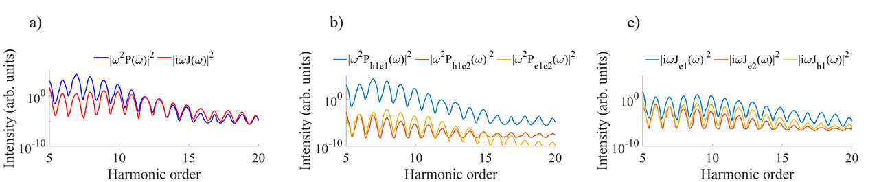
Figure 1: a) Total interband polarization and intraband current. b) Separate contributions of the interband polarization. c) Separate contributions of the intraband current.

Three selection rules must be considered to understand non-collinear wave mixing spectra driven by the fundamental and its second harmonic, and to assign each harmonic order to a unique combination of photons. Both wavelengths contribute to the emitted photon energies via an integer number of photons. From a simple energy conservation standpoint, the expected emission takes place at photon energies: $q\omega_{f}=n\omega_{f}+m2\omega_{f}=(n+2m)\omega_{f}$, where $q=n+2m$ is the harmonic order, $\omega_{f}$ is the angular frequency of the fundamental laser field, and $n$ and $m$ are the numbers of photons from the fundamental and its second harmonic, respectively. This yields a discrete spectrum, shown in Fig. 1b. Emission corresponding to even harmonics of the fundamental is present, despite the fact that fused silica is a centrosymmetric material. In fact, in a two-color field of commensurate frequencies, the parity conservation rule, which requires the total number of photons $n+m=$ to be odd, allows for generation of even harmonics of the fundamental through the addition (subtraction) of an odd amount of photons. The third conservation rule needed for a description of the full far-field profile shown in Fig. 1b, is conservation of the momentum. The harmonic spectrum spans less then an octave in energy, resulting into a unique mapping of each wave-mixing order (WMO) onto its emission angle $\beta$ for a crossing angle $\alpha$ between fundamental and the second harmonic,

$$\beta(n,m)=\frac{2m\sin\alpha}{n+2m\cos\alpha}.$$ (1)

A small-angle approximation is used in Eq. 1. Similar concepts have previously been applied in gas-phase HHG Bertrand et al. (2011); Heyl et al. (2014).

II Theory of high-order wave-mixing spectra

II.1 Semiconductor Bloch equations

We model the generation of high-harmonics from silica, by solving the semiconductor Bloch equations Lindberg and Koch (1988); Golde et al. (2008); Schubert et al. (2014) for a three-level system, consisting of one valance band and two conduction bands. Throughout this manuscript we use atomic units. The system of coupled differential equations are solved for the momentum $k$ dependent population $f^{\lambda}_{k}$ in band $\lambda$ and the polarization $p^{\lambda\lambda^{\prime}}_{k}$ between bands $\lambda$ and $\lambda^{\prime}$, and is written out for bands $\lambda\in\{h_{1},e_{1},e_{2}\}$ as:

$$i\frac{\partial}{\partial t}p^{h_{1}e_{1}}_{k}=(\epsilon^{e_{1}}_{k}+\epsilon^{h_{1}}_{k}-i\frac{1}{T_{2}})p^{h_{1}e_{1}}_{k}-(1-f^{e_{1}}_{k}-f^{h_{1}}_{k})d^{e_{1}h_{1}}_{k}F(t)+iF(t)\cdot\nabla_{k}p^{h_{1}e_{1}}_{k}+F(t)[d^{e_{2}h_{1}}_{k}p^{e_{2}e_{1}}_{k}-d^{e_{1}e_{2}}_{k}p^{h_{1}e_{2}}_{k}]$$ (2)

$$i\frac{\partial}{\partial t}p^{h_{1}e_{2}}_{k}=(\epsilon^{e_{2}}_{k}+\epsilon^{h_{1}}_{k}-i\frac{1}{T_{2}})p^{h_{1}e_{2}}_{k}-(1-f^{e_{2}}_{k}-f^{h_{1}}_{k})d^{e_{2}h_{1}}_{k}F(t)+iF(t)\cdot\nabla_{k}p^{h_{1}e_{2}}_{k}+F(t)[d^{e_{1}h_{1}}_{k}p^{e_{2}e_{1}}_{k}-d^{e_{1}e_{2}}_{k}p^{h_{1}e_{1}}_{k}]$$ (3)

$$i\frac{\partial}{\partial t}p^{e_{1}e_{2}}_{k}=(\epsilon^{e_{2}}_{k}-\epsilon^{e_{1}}_{k}-i\frac{1}{T_{2}})p^{e_{1}e_{2}}_{k}+(f^{e_{2}}_{k}-f^{e_{1}}_{k})d^{e_{2}e_{1}}_{k}F(t)+iF(t)\cdot\nabla_{k}p^{e_{1}e_{2}}_{k}+F(t)[d^{e_{1}h_{1}}_{k}p^{e_{2}h_{1}}_{k}-d^{h_{1}e_{2}}_{k}(p_{k}^{h_{1}e_{1}})^{*}]$$ (4)

$$\frac{\partial}{\partial t}f^{e_{1}}_{k}=-2~{}\text{Im}[d^{e_{1}e_{2}}_{k}F(t)(p^{e_{2}e_{1}}_{k})^{*}+d^{e_{1}h_{1}}_{k}F(t)(p^{h_{1}e_{1}}_{k})^{*}]+F(t)\cdot\nabla_{k}f^{e_{1}}_{k}.$$ (5)

$$\frac{\partial}{\partial t}f^{e_{2}}_{k}=-2~{}\text{Im}[d^{e_{2}e_{1}}_{k}F(t)(p^{e_{1}e_{2}}_{k})^{*}+d^{e_{2}h_{1}}_{k}F(t)(p^{h_{1}e_{2}}_{k})^{*}]+F(t)\cdot\nabla_{k}f^{e_{2}}_{k}.$$ (6)

$$\frac{\partial}{\partial t}f^{h_{1}}_{k}=-2~{}\text{Im}[d^{e_{1}h_{1}}_{k}F(t)(p^{h_{1}e_{1}}_{k})^{*}+d^{e_{2}h_{1}}_{k}F(t)(p^{h_{1}e_{2}}_{k})^{*}]+F(t)\cdot\nabla_{k}f^{h_{1}}_{k}.$$ (7)

in which, the single particle energies of the carriers in band $\lambda$ are given by $\epsilon_{k}^{\lambda}$. The creation of polarization and population due to the presence of an electric field $F(t)$ follows from the terms that involve the transition dipole moment $d^{\lambda\lambda^{\prime}}_{k}$. The intraband dynamics, caused by carrier acceleration by $F(t)$ within the bands, are described by the terms including $\nabla_{k}$. The dephasing time of the polarization is denoted by $T_{2}$. The transition dipole moment $d^{\lambda\lambda^{\prime}}_{k}$ between the bands $\lambda$ and $\lambda^{\prime}$ is approximated in first order $\textbf{k}\cdot\textbf{p}$ theory Haug and Koch (2009) as

$$d^{\lambda\lambda^{\prime}}_{k}=d_{0}^{\lambda\lambda^{\prime}}\frac{E_{g}^{\lambda\lambda^{\prime}}}{\epsilon_{k}^{\lambda}-\epsilon_{k}^{\lambda^{\prime}}},$$ (8)

where $d_{0}^{\lambda\lambda^{\prime}}$ resembles the transition dipole moment between bands $\lambda$ and $\lambda^{\prime}$ at the -point, and $E_{g}^{\lambda\lambda^{\prime}}$ the bandgap energy at the -point between bands $\lambda$ and $\lambda^{\prime}$. The semiconductor Bloch equations are cast as a set of coupled partial differential equations with periodic boundaries. To solve this numerical problem, the k-dimension of the equations are represented in a Fourier-series base and then solved by using spectral methods, as provided through the Dedalus project Burns et al. (2020).

The macroscopic polarization $P(t)$ and macroscopic current $J(t)$ are calculated Golde et al. (2008) by

$$P(t)=\sum_{\lambda,\lambda^{\prime},k}[d^{\lambda\lambda^{\prime}}_{k}p^{\lambda\lambda^{\prime}}_{k}+c.c.]$$ (9)

$$J(t)=\sum_{\lambda,k}v^{\lambda}(k)f^{\lambda}_{k}$$ (10)

with the group velocity $v^{\lambda}(k)$ given by

$$v^{\lambda}(k)=\nabla_{k}\epsilon^{\lambda}_{k}.$$ (11)

We calculate the spectral representation of the source field of interband polarization and intraband current as follows

$$F_{\mathrm{inter}}(\omega)=\mathcal{F}[\frac{\partial}{\partial t}j_{\mathrm{inter}}(t)]=\mathcal{F}[\frac{\partial^{2}}{\partial^{2}t}P(t)]=\omega^{2}\mathcal{F}[P(t)]=\omega^{2}P(\omega).$$ (12)

and the current as

$$F_{\mathrm{intra}}(\omega)=\mathcal{F}[\frac{\partial}{\partial t}j_{\mathrm{intra}}(t)]=i\omega\mathcal{F}[J(t)]=i\omega J(\omega).$$ (13)

The harmonic spectral density at the sample plane is then defined as

$$I_{\mathrm{HHG}}(\omega)=|\omega^{2}P(\omega)+i\omega J(\omega)|^{2}.$$ (14)

II.2 Far-field propagation

The SBE yield the spatial distribution of the complex electric field for the interband and intraband contributions $F_{\mathrm{inter}}(\omega)$ and $F_{\mathrm{intra}}(\omega)$, respectively, at the sample plane. Detection is performed in the far-field which, in the Fraunhofer diffraction regime, is related to the sample plane through a Fourier transform:

$$\mathcal{F}[F_{\mathrm{HHG}}(x_{SP},\omega)]\propto F_{\mathrm{HHG}}(x_{FF},\omega).$$ (15)

The field at the sample plane is described by a one-dimensional spatial variable $x_{SP}$. To obtain a far-field pattern, the harmonic signal $F_{\mathrm{HHG}}=F_{\mathrm{inter}}+F_{\mathrm{intra}}$ is computed for every value of $x_{SP}$. The near-field spectrum of the solid HHG is propagated to the far-field by Fraunhofer diffraction, which gives the wave mixing pattern shown in Fig. 2(b) in the main text. The total field is built up by an 800-nm pulse and a 400-nm pulse, which are crossed under an angle $\beta$, thus creating a time-dependent grating-like interference pattern. The FWHM size of the focus of the 800-nm pulse is measured to be 170 µm, the 400-nm focus is measured to be 70 µm. In the focal plane both pulses are assumed to have a flat spatial phase front. The only remaining phase factor is introduced by the angle $\beta$ between the two pulses, which depends on the position x, $\phi(x)\approx x\sin(\beta)$.

II.3 Separation into band-resolved interband-polarization and intraband-current contributions

The total harmonic signal in the wavemixing configuration of Fig. 2b (main text) is calculated by summing up all contributions along the sample plane, see Fig. S1a. To identify which bands contribute most to the signal, we calculate the separate values of the interband polarization (Fig. S1b) and the intraband current (Fig. S1c)). Overall, the polarization dominates the emission in the spectral region around the bandgap (H5-H11). The main contribution of the intraband current originates from the carriers inside the first conduction band. The main contribution of the polarization is generated between the valence and the lowest lying conduction band.

II.4 Electronic-structure calculations for material parameters of Silica

The energy levels and the transition dipole moments of fused silica at the -point between the valence band and two conduction bands are calculated within density functional theory, using pseudopotentials (generalised gradient approximation in the shape of the Perdew, Burke, and Ernzerhof (PBE) functional Perdew et al. (1996)) and a plane-wave basis set as implemented in Quantum Espresso Giannozzi et al. (2017). The plane-wave energy cutoff used was 40 Ry. The calculation is performed for an automatically generated uniform grid of 10 points in each k direction. Both these parameters were tested for convergence. The energy levels at $\mathrm{k=0}$ are calculated to be 0 eV, 9.6 eV and 12.6 for the valence and the two lowest lying conduction bands respectively. The dipole moments between these energy levels $\lambda,\lambda^{\prime}$ are calculated to be $d_{0}^{h_{1}e_{1}}=0.318$ a.u., $d_{0}^{e_{1}e_{2}}=0.014$ a.u. and $d_{0}^{e_{2}h_{1}}=0.037$ a.u., using the epsilon function from the post processing data package. The dispersion relation of the bands of silica are taken from Luu et al. (2015). We model the light-matter interaction along the $\Gamma$-M crystal direction of quartz, as this orientation generates the most harmonic emission Luu et al. (2015).

II.5 Semiclassical description of laser-driven carrier motion

The semiclassical description Wegener (2005); Luu et al. (2015) of the carrier dynamics inside an energy band $\lambda$ starts with describing the velocity of an electronic wavepacket by

$$\textbf{v}^{\lambda}(\textbf{k},t)=\frac{\partial\epsilon^{\lambda}(\textbf{k})}{\partial\textbf{k}}.$$ (16)

The crystal momentum is time-dependent, given by

$$\textbf{K}(t)=\textbf{k}+\textbf{A}(t),$$ (17)

with the vector potential,

$$\textbf{A}(t)=-\int_{\infty}^{t}\textbf{F}(t^{\prime})dt^{\prime}$$ (18)

based on the two-color laser field $\textbf{F}(t)=F_{800}\cos(\omega t)+F_{400}\cos(2\omega t+\phi)$, with the field amplitudes of the fundamental ($F_{800}$) and second harmonic ($F_{400}$) field, and the relative phase $\phi$ between the fields. By expressing the dispersion relation of band $\lambda$ as,

$$\epsilon^{\lambda}(\textbf{k})=\sum_{\textbf{r}}E^{\lambda}(\textbf{r})\cos(\textbf{k}\cdot\textbf{r})$$ (19)

in which the band coefficients $E^{\lambda}(\textbf{r})$ represent the amplitude of the spatial harmonics of the lattice structure, and by substituting the time-dependent crystal momentum we obtain a final expression for the velocity

$$\textbf{v}^{\lambda}(\textbf{k},t)=-\sum_{\textbf{r}}\textbf{r}E^{\lambda}(\textbf{r})\sin[(\textbf{k}+\textbf{A}(t))\cdot\textbf{r}].$$ (20)

We calculate the harmonic intensity as

$$I_{\mathrm{HHG}}(\omega)\propto\sum_{\textbf{k}}|\omega\mathcal{F}[\textbf{v}^{\lambda}(\textbf{k},t)]|^{2}.$$ (21)

To reproduce the intensity scalings, we calculate the spectrum for each combination of intensities of the fundamental and second harmonic in Fig. 3 of the main text. The semiconductor Bloch simulations reveal that the main contribution is coming from the polarization between the valence band and the first conduction band. In addition, the nonlinearity of the valence band is much lower than for the first conduction band, such that the main emission will originate from the first conduction band. Therefore we calculate the spectrum used in the intensity scalings only based on the dispersion relation of the first conduction band.

III Additional experimental data and analysis

III.1 Intensity scaling of the harmonic yield

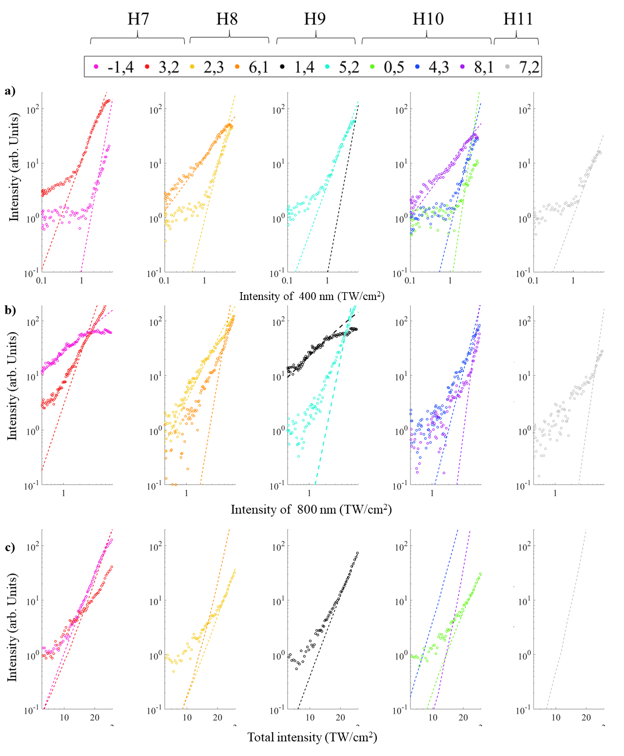
Figure 2: Comparison between experimental data (open circles) and simulations (dashed lines). a) The intensity of the 800-nm pulse is 11.0 TW/cm². b) The intensity of the 400-nm pulse is 5.4 TW/cm². c) The ratio of the intensities of the 800-nm pulse over that of the 400-nm pulse is 1:3.5.

The experimental intensity is calculated using the measured pulse length, refractive index of the material, focus size and pulse energy. The pulse length for the fundamental pulse was determined by a home-built frequency-resolved optical gating (FROG) setup and the focus sizes were measured outside the chamber, where focal overlap was maximum. Figure S2 shows all measured WMOs, a selection of those is shown in Fig. 3. The measured data is displayed as circles and the simulated data, based on the semiclassical description of laser-driven carrier motion (SI, section II.E), as dashed lines. Not all experimental intensity scalings show all WMOs, since the appearance of WMOs depends on the combination of fundamental and 400-nm intensity used. For the scaling of the 400-nm pulse intensity, we observe that for all WMOs there are intensity ranges which are accurately described by a perturbative power scaling. As mentioned in the main text, during the intensity scaling of the fundamental pulse (see Fig. S2b), the overlap between both two foci may have deteriorated for higher intensities due to a thermal drift. This leads to an overestimation of the fundamental intensity involved in the wavemixing, and therefore shows deviating power laws at higher intensities.

III.2 Enhancement factors

In all experimental scans the WMOs show the highest signal compared to the on-axis harmonic orders. In order to estimate how much brighter the WMOs are, we compare the yield of a WMO with the yield of an on-axis harmonic generated at the same photon energy and total intensity, see Fig. S3. To obtain the fairest comparison, we compare scans where HHG is exclusively driven by the fundamental 800 nm pulses and in which the total intensity is build up from both driving wavelengths. Both scans were taken under similar experimental conditions.

More specifically, we compare scans where the intensity of the 800-nm pulse is around 11.0 TW/cm² and the intensity of the 400-nm pulse is varied (blue lines in Fig. S3). At this 800 nm intensity, the efficiency of HHG driven by 800 nm alone is close to maximal and the main on-axis harmonics (orders (7,0), (9,0), and (11,0)) are always present, and their yield does not change significantly by addition of the second color. Scans in which the intensity of the 800-nm pulses is scaled and the intensity of 400 nm is kept constant (red lines in Fig. S3) start at lower intensity of the 800 nm pulses and the WMOs show a dramatic increase in yield. Comparing the yield of the WMOs as a function of total driving intensity (fundamental and SH intensity combined) with the yield of on-axis harmonic orders at the same photon energy and total driving intensity, provides the enhancement factors. The yield of order (7,0) is only a few arbitrary units at an intensity of 11.0 TW/cm². At the same total intensity, which now consist of both fundamental and SH intensity, the signal of WMO (3,2) has a yield of about 170 (arbitrary units), leading to an enhancement factor of 85. An enhancement factor of about 50 is found for H9, shown in Fig. S3b, in which the on-axis harmonic (9,0) has a single-digit yield, whereas the WMO (5,2) shows a yield of around 100. For H11 the enhancement is least pronounced, the signal of the WMO (7,2) is about 7 times larger then the on-axis harmonic (11,0). Overall we are confident to report an increase of the WMOs with at least one and up to two orders of magnitude compared to the on-axis harmonics for H7 and H9, and about half an order of magnitude for H11.

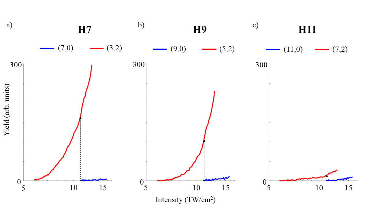
Figure 3: The yield of several harmonic orders (of the fundamental) at a) 10.9 eV, b) 14.0 eV, and c) 17.1 eV photon energy, as a function of total driving intensity. The blue curves represent on-axis harmonics, in which the 800-nm intensity is fixed around 11.0 TW/cm² and the 400-nm intensity is increased from 0 TW/cm² to about 5 TW/cm². The red curves represent WMOs at the same photon energies (10.9 eV, 14.0 eV, and 17.1 eV, respectively) in which the 400-nm intensity is fixed around 5.4 TW/cm² and the 800-nm intensity is increased from 0 to 7.5 TW/cm².

References

- Bertrand et al. (2011) J. Bertrand, H. J. Wörner, H.-C. Bandulet, É. Bisson, M. Spanner, J.-C. Kieffer, D. Villeneuve, and P. B. Corkum, Phys. Rev. Lett 106, 023001 (2011).
- Heyl et al. (2014) C. M. Heyl, P. Rudawski, F. Brizuela, S. N. Bengtsson, J. Mauritsson, and A. L’Huillier, Phys. Rev. Lett. 112, 1 (2014).
- Lindberg and Koch (1988) M. Lindberg and S. W. Koch, Phys. Rev. B 38, 3342 (1988).
- Golde et al. (2008) D. Golde, T. Meier, and S. W. Koch, Phys. Rev. B 77, 075330 (2008).
- Schubert et al. (2014) O. Schubert, M. Hohenleutner, F. Langer, B. Urbanek, C. Lange, U. Huttner, D. Golde, T. Meier, M. Kira, S. W. Koch, et al., Nat. Photonics 8, 119 (2014).
- Haug and Koch (2009) H. Haug and S. W. Koch, Quantum theory of the optical and electronic properties of semiconductors (World Scientific Publishing Company, 2009).
- Burns et al. (2020) K. J. Burns, G. M. Vasil, J. S. Oishi, D. Lecoanet, and B. P. Brown, Phys. Rev. Res. 2, 023068 (2020).
- Perdew et al. (1996) J. P. Perdew, K. Burke, and M. Ernzerhof, Physical review letters 77, 3865 (1996).
- Giannozzi et al. (2017) P. Giannozzi, O. Andreussi, T. Brumme, O. Bunau, M. B. Nardelli, M. Calandra, R. Car, C. Cavazzoni, D. Ceresoli, M. Cococcioni, et al., J. Condens. Matter Phys 29, 465901 (2017), URL http://stacks.iop.org/0953-8984/29/i=46/a=465901.
- Luu et al. (2015) T. T. Luu, M. Garg, S. Y. Kruchinin, A. Moulet, M. T. Hassan, and E. Goulielmakis, Nature 521, 498 (2015).
- Wegener (2005) M. Wegener, Extreme nonlinear optics: an introduction (Springer Science & Business Media, 2005).