Quantum effects in two-dimensional silicon carbide

Abstract

Two-dimensional (2D) silicon carbide is an emergent direct band-gap semiconductor, recently synthesized, with potential applications in electronic devices and optoelectronics. Here, we study nuclear quantum effects in this 2D material by means of path-integral molecular dynamics (PIMD) simulations in the temperature range from 25 to 1500 K. Interatomic interactions are modeled by a tight-binding Hamiltonian fitted to density-functional calculations. Quantum atomic delocalization combined with anharmonicity of the vibrational modes cause changes in structural and thermal properties of 2D SiC, which we quantify by comparison of PIMD results with those derived from classical molecular dynamics simulations, as well as with those given by a quantum harmonic approximation. Nuclear quantum effects are found to be appreciable in structural properties such as the layer area and interatomic distances. Moreover, we consider a real area for the SiC sheet, which takes into account bending and rippling at finite temperatures. Differences between this area and the in-plane area are discussed in the context of quantum atomic dynamics. The bending constant ($\kappa=1.0$ eV) and the 2D modulus of hydrostatic compression ($B_{xy}$ = 5.5 eV/Ų) are clearly lower than the corresponding values for graphene. This study paves the way for a deeper understanding of the elastic and mechanical properties of 2D SiC.

Keywords: Silicon carbide, quantum effects, molecular dynamics

I Introduction

Bulk silicon carbide has been known for many years as a material with remarkable physical properties, such as low density, high thermal conductivity, low thermal expansion, high strength, and high refractive index Melinon et al. (2007). This material is known in more than 250 different polytypes, many of them with hexagonal crystalline structure. In recent years, several new materials containing both silicon and carbon have been studied. Among them, one finds fullerenes, nanotubes, and two-dimensional (2D) structures Melinon et al. (2007); Hsueh et al. (2011); Shi et al. (2015); Bekaroglu et al. (2010). In particular, great progress has been lately made in the understanding and synthesis of 2D SiC Lin (2012); Chabi et al. (2016); Huelmo and Denis (2019); Chabi et al. (2021), which turns out to be a direct wide band-gap semiconductor with potential applications in electronic devices and optoelectronics Susi et al. (2017); Chabi and Kadel (2020); Drissi et al. (2020); Guo et al. (2018). Specifically, this material has valuable optical properties as large photoluminescence intensity and excitonic effects, due to its direct band-gap and electronic quantum confinement Chabi and Kadel (2020); Hsueh et al. (2011).

Several compositions Si_xC_1-x for 2D silicon carbide have been predicted to be also stable, and to behave as semiconductor, semimetal, or topological insulators, depending on the stoichiometry Shi et al. (2015); Chabi and Kadel (2020); Fan et al. (2017). The lowest formation energy has been found for the isoatomic stoichiometry Si_0.5C_0.5, which we call 2D SiC Shi et al. (2015).

Understanding structural and thermal properties of two-dimensional systems has been a goal in statistical physics for many years Safran (1994); Nelson et al. (2004); Tarazona et al. (2013), above all in the context of biological membranes and soft condensed matter Fournier and Barbetta (2008); Tarazona et al. (2013). This problem has expanded its interest to crystalline membranes, after the synthesis of graphene and related materials in recent years. Dealing with crystalline 2D materials allows us to reliably model systems at the atomic scale, opening an access to physical properties of this kind of systems Pop et al. (2012); Fong et al. (2013); Wang et al. (2016); Herrero and Ramírez (2018). In this context, electronic structure methods have been used since the 1980s to study equilibrium configurations, energetics, quantum-size effects, and related aspects of ordered 2D systems Mintmire et al. (1982); Feibelman and Hamann (1984); Boettger (1988); Boettger et al. (1990); Trickey et al. (1992).

Electronic structure calculations of 2D SiC have shown features of the minimum-energy configuration for this layered material, which turns out to be planar. At finite temperatures, one expects the presence of bending and ripping in the SiC layer, as has been studied earlier for graphene. Moreover, quantum effects such as zero-point motion will cause atomic delocalization and departure of strict planarity, even at $T=0$. Also, nuclear quantum effects can be important for vibrational and electronic properties of relatively light atomic species such as carbon, as has been shown earlier for graphene, mainly at low temperatures.

Path-integral simulations (molecular dynamics and Monte Carlo) are well suited to appraise effects associated to the quantum character of atomic nuclei. This kind of simulations allow us to efficiently quantize the nuclear degrees of freedom, including both thermal and quantum fluctuations at finite temperatures Gillan (1988); Ceperley (1995). This procedure allows one to carry out quantitative analyses of anharmonic effects in condensed matter Herrero and Ramírez (2016); Brito et al. (2019).

In this paper we employ the path-integral molecular dynamics (PIMD) procedure to study nuclear quantum effects in vibrational, structural, and thermal properties of 2D SiC in a temperature range from from 25 to 1500 K. Interatomic interactions are obtained from a tight-binding (TB) Hamiltonian, built up according to results of calculations based on density-functional theory (DFT). Path-integral simulation analogous to those carried out here were used earlier to analyze nuclear quantum effects in carbon-based materials such as diamond Ramírez et al. (2006); Brito et al. (2020) and graphite Herrero and Ramirez (2021a), as well as in silicon Noya et al. (1996). This kind of techniques have been applied in recent years to study 2D materials as graphene Brito et al. (2015); Hasik et al. (2018); Herrero and Ramírez (2016) and BN Brito et al. (2022). Here we will discuss similarities and differences of 2D SiC with other 2D materials, especially graphene.

The paper is organized as follows. In Sec. II we explain the computational procedures used here: PIMD technique and tight-binding method. In Sec. III we give results obtained in a harmonic approximation of the vibrational modes in 2D SiC. In Sec. IV we present results for the internal energy derived from PIMD simulations, as well as its constituent parts, kinetic and potential energy. Interatomic distances and atomic mean-squares displacements are discussed in Secs.  V and VI, respectively. A discussion on the layer area (in-plane and real) is given in Sec.  VII. The paper closes with a Summary of the main results.

II Method of calculation

II.1 Path-integral molecular dynamics

The Feynman path-integral formulation of statistical physics Feynman (1972) is a well established tool to study many-body quantum systems at finite temperatures. This method is nowadays employed to study properties of condensed matter by means of its implementation in numerical simulations using Monte Carlo or molecular dynamics techniques. In this paper we use the path-integral molecular dynamics (PIMD) method to study the influence of nuclear quantum effects on structural and vibrational properties of 2D silicon carbide at several temperatures. In this section we give some details on this computational procedure, pertinent for the presentation of our results for 2D-SiC. More details on this kind of atomistic simulations are given elsewhere Ceperley (1995); Gillan (1988); Tuckerman (2010); Herrero and Ramírez (2014).

Our simulations are carried out in the isothermal-isobaric ensemble with variables $N$ (number of particles), $\tau$ (in-plane stress), and $T$ (temperature). We consider a simulation cell with $N/2$ carbon and $N/2$ silicon atoms. We take $\tau=0$, so that the external stress on the SiC layer vanishes. $\tau$ (with units of force per unit length), is the conjugate variable to the in-plane area $A_{p}$, which in the following will be the area of the simulation cell on the $(x,y)$ plane.

The partition function $Z(N,\tau,T)$ for the isothermal-isobaric ensemble is given by

$$Z(N,\tau,T)=\int dA_{p}\,\exp(-\beta\tau A_{p})\,Z(N,A_{p},T)\,,$$ (1)

where $Z(N,A_{p},T)$ is the canonical partition function, $\beta=1/(k_{B}T)$, and $k_{B}$ is Boltzmann’s constant. Using the Trotter formula and a high-temperature approximation for the density matrix Gillan (1988); Kleinert (1990); Herrero and Ramírez (2014), $Z(N,A_{p},T)$ can be written for our SiC layer system as

$$Z(N,A_{p},T)\approx\left(\frac{M_{\rm C}^{1/2}M_{\rm Si}^{1/2}P}{2\pi\beta{\hbar}^{2}}\right)^{3PN/2}\\ \int d{\bf R}_{1}\dots d{\bf R}_{P}\;\exp\left[-\beta\;V_{\text{eff}}({\bf R}_{1},...,{\bf R}_{P})\right]\,.$$ (2)

Here, ${\bf R}_{p}\,(p=1,...,P)$ is a $3N$-dimensional vector, whose components are the Cartesian coordinates of the atomic nuclei $({\bf r}_{1,p},...,{\bf r}_{N,p})$. The index $p$ indicates the path coordinate, which is discretized into $P$ points (Trotter number) along a path, and the cyclic condition imposes ${\bf R}_{P+1}={\bf R}_{1}$. $M_{\rm C}$ and $M_{\rm Si}$ are the atomic masses of C and Si, respectively.

Thus, $Z(N,A_{p},T)$ is equivalent to the canonical partition function of a classical system with an effective potential:

$$V_{\text{eff}}({\bf R}_{1},...,{\bf R}_{P})=\frac{P}{2\beta^{2}{\hbar}^{2}}\sum_{j=1}^{N}\sum_{p=1}^{P}M_{j}({\bf r}_{j,p+1}-{\bf r}_{j,p})^{2}+\\ +\frac{1}{P}\sum_{p=1}^{P}V({\bf R}_{p})\;,$$ (3)

where $j$ runs over the $N$ atomic nuclei, $M_{j}=M_{\rm C}$ for $j\leq N/2$, and $M_{j}=M_{\rm Si}$ for $j>N/2$. $V_{\text{eff}}({\bf R}_{1},...,{\bf R}_{P})$ corresponds to the interaction potential of a classical system made up of $N$ cyclic chains (one per atomic nucleus), where successive elements (beads) are coupled by a harmonic interaction with force constant $\kappa_{j}={M_{j}P}/{\beta^{2}{\hbar}^{2}}$ (first term on the r.h.s. of Eq. (3)). The interchain coupling is restricted to beads with the same index $j$, and corresponds to interaction potential $V({\bf R}_{p})$ for $p=1,...,P$. Here, this potential is derived from a tight-binding (TB) Hamiltonian, as explained below in Sec. II.B. The expression for $Z(N,A_{p},T)$ in Eq. (2) is exact in the limit $P\rightarrow\infty$, and it is valid for distinguishable particles, which is justified for C and Si nuclei in the considered 2D crystalline membrane, since the overlap of nuclear wave functions is negligible.

To have a roughly constant accuracy for the results at different temperatures, we have taken a Trotter number which scales as the inverse temperature. At a given temperature, the value of $P$ needed to obtain convergence of the results depends on the scale of the vibrational frequencies in the material. We have taken $PT=6000$ K. For example, a PIMD simulation for $N$ = 112 atoms at $T$ = 50 K ($P$ = 120), requires dealing with $NP$ = 13,440 classical particles. The finite Trotter number $P$ causes the appearance of a cutoff for the vibrational energy. In fact, the largest energy sampled using $P$ amounts to $E_{c}\approx\hbar/\epsilon$, with $\epsilon=\beta\hbar/P$. This translates into a cutoff for the vibrational frequencies at $\omega_{c}=Pk_{B}T/\hbar\approx 4200$ cm^-1, much larger than the frequencies appearing in 2D SiC (see below).

We employed algorithms for performing PIMD simulations in the $N\tau T$ ensemble, as those given in the literature Martyna et al. (1999); Tuckerman (2010). In particular, we have used staging variables to define the bead coordinates, and the constant-$T$ ensemble has been obtained by coupling chains of Nosé-Hoover thermostats to each staging variable. In addition, a barostat chain was coupled to the in-plane area of the simulation cell to keep an in-plane stress $\tau=0$ Tuckerman (2010); Herrero and Ramírez (2014). The equations of motion were integrated through the reversible reference system propagator algorithm (RESPA), allowing us to use different time steps for the integration of fast and slow degrees of freedom Martyna et al. (1996). On one side, for the atomic dynamics associated to interatomic forces, we used a time step $\Delta t$ = 1 fs. On the other side, we considered a time step $\delta t=\Delta t/4$, for the evolution of fast dynamical variables, i.e., thermostats and harmonic bead interactions. The equations of motion employed in our simulations, specific for 2D materials, are given in detail elsewhere Ramírez and Herrero (2020). The dynamics in this computational method does not correspond to the real quantum dynamics of the actual particles, but it is accurate for sampling the true many-body configuration space, thus giving precise values for time-independent equilibrium variables of the considered quantum system.

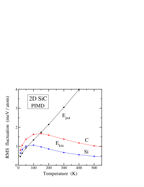
Figure 1: RMS fluctuations of the kinetic and potential energy for 2D SiC as a function of temperature, as derived from PIMD simulations. Circles: potential energy; squares: kinetic energy of carbon; diamonds: kinetic energy of silicon. Error bars are less than the symbol size. Curves are guides to the eye.

The kinetic energy, $E_{\rm kin}$, has been obtained by using the so-called virial estimator, which has a statistical uncertainty less than the potential energy of the system, mainly at high temperature Herman et al. (1982); Tuckerman (2010). This estimator helps to determine the mean kinetic energy with good accuracy. In Fig. 1 we present the root mean-square (RMS) fluctuations of the kinetic energy ($E_{\rm kin}$) obtained with this procedure in our PIMD simulations of 2D SiC, as well as those of the potential energy ($E_{\rm pot}$) of the system up to 500 K. On one side, one observes that RMS fluctuations of $E_{\rm pot}$ grow as $T$ is raised, and in fact at high $T$ we find an approximately linear increase, as expected for thermodynamic fluctuations of a classical system in the $N\tau T$ ensemble. On the other side, the RMS fluctuations of $E_{\rm kin}$ obtained for the virial estimator attain a maximum at about 100 K for Si and 150 K for C and decrease at higher $T$.

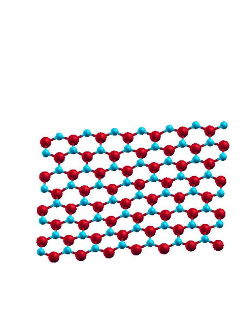
Figure 2: Snapshot taken from a simulation of 2D silicon carbide at $T=300$ K. Large red and small light blue spheres indicate silicon and carbon atoms, respectively.

For the simulations presented here, we have taken rectangular simulation cells with similar side length in the $x$ and $y$ directions of the $(x,y)$ reference plane ($L_{x}\approx L_{y}$), where periodic boundary conditions were considered. In the out-of-plane $z$-direction, free boundary conditions were assumed, so Si and C atoms can move without restriction, as in a free-standing layer. We considered simulation cells with $N$ = 112 atoms, at temperatures between 25 and 1500 K. To check the convergence of our results with system size, some calculations were carried out for $N$ up to 308 atoms. Given a temperature, a typical simulation run consisted of $10^{5}$ PIMD steps for system equilibration, followed by $4\times 10^{6}$ steps for the calculation of ensemble average properties. In Fig. 2 we present a view of a 2D SiC configuration obtained in our simulations at $T=300$ K. In this picture, large red and small light blue spheres represent C and Si atoms, respectively.

To quantify the magnitude of quantum effects in the equilibrium properties of 2D SiC, some classical molecular dynamics (MD) simulations have been also performed with the same TB Hamiltonian. In our context of path-integral simulations, the classical limit is obtained from Eq. (3) by putting $P=1$ (in this case, the first term on the r.h.s. disappears).

II.2 Tight-binding method

Our simulations were performed within the adiabatic (Born-Oppenheimer) approximation, which allows one to define a potential-energy surface for the nuclear dynamics. We obtain the Born-Oppenheimer surface from an effective tight-binding Hamiltonian, based on density functional calculations Porezag et al. (1995). Thus, our procedure takes into account the quantum nature of both, electrons and atomic nuclei, the former through the TB Hamiltonian and the latter by means of path integrals. In this way, phonon-phonon and electron-phonon interactions are directly included in our PIMD simulations.

Total energies and interatomic forces are calculated in our simulations using the DFT based non-orthogonal TB Hamiltonian of Porezag et al. Porezag et al. (1995). In particular, the TB parametrization for structures containing Si and C atoms was presented in Ref. Gutierrez et al. (1996). The main steps for this parametrization are: i) atomic orbitals are derived as the eigenfunctions of appropriately constructed pseudoatoms, where the charge density of the valence electrons is concentrated closer to the nucleus; ii) overlap matrices between the atomic orbitals are tabulated as a function of the internuclear distance; iii) matrix elements of the TB Hamiltonian are calculated using DFT in the local density approximation (LDA), and tabulated also as a function of the internuclear distance; iv) finally, a short-range repulsive part of the total potential is fitted to self-consistent-field LDA data of proper reference systems. The non-orthogonality of the atomic basis is an important key for the transferability of the parametrization to complex systems Porezag et al. (1995). This TB method is not self-consistent and, contrary to other empirical TB approaches, it does not include any temperature effect or any fit to experimental data in its parametrization.

The TB model used in this paper was employed earlier to analyze the (1x1) reconstruction of the (110) SiC surface Gutierrez et al. (1996), to study nuclear quantum effects in 3C SiC Ramírez et al. (2008), and to investigate isotope effects in this 3D material Herrero et al. (2009). A detailed review on the ability of TB methods to precisely describe several properties of solids and molecules was presented by Goringe et al. Goringe et al. (1997).

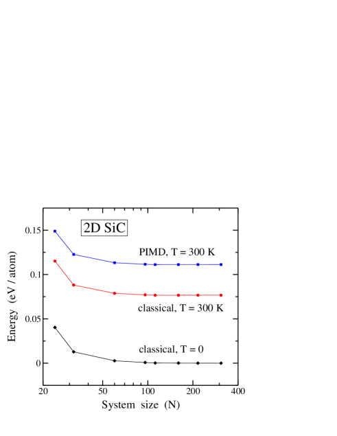
Figure 3: Potential energy of 2D SiC for various simulation cell sizes ($N$). Diamonds: classical, $T=0$; circles: classical, $T=300$ K; squares: quantum, $T=300$ K. The zero of energy is taken from the $T=0$ classical result for $N=308$. Error bars are less than the symbol size. Note the logarithmic scale in the horizontal axis.

For the reciprocal-space sampling of electronic degrees of freedom we considered only the $\Gamma$ point (${\bf k}=0$), since the main effect of using larger ${\bf k}$ sets is a shift in the total energy, with negligible effect on the calculation of energy differences. A similar effect appears for the energy as a function of the simulation-cell size. This is shown in Fig. 3, where we display the convergence of the potential energy of 2D SiC for several cell sizes $N$. The data points correspond to $E_{\rm pot}$ calculated with the TB model ($\Gamma$ point) for the minimum-energy configuration (classical, $T=0$). In this figure, we also present results for the energy obtained for several cell sizes from classical MD (circles) and PIMD simulations (squares) at $T$ = 300 K. In both cases, we observe a rigid energy shift with respect to the classical calculations at $T=0$.

III Harmonic approximation

For the sake of comparison with the results of our PIMD simulations of 2D SiC, we present here a harmonic approximation (HA) for the atomic vibrational modes. Such an approximation in condensed matter is usually rather precise at low temperatures. Anharmonicity appears as temperature increases, and the outcomes of the HA gradually deviate from those obtained for more realistic atomistic simulations. In the HA, vibrational frequencies are assumed to be constant (independent of the temperature, i.e., those derived for the minimum-energy configuration), and changes in the in-plane area $A_{p}$ with temperature are not taken into account. Thus, we are not considering a quasi-harmonic approximation Ashcroft and Mermin (1976); Debernardi and Cardona (1996), where frequencies can change with temperature, which can be useful for some calculations not addressed here.

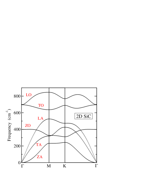
Figure 4: Phonon dispersion bands of 2D silicon carbide, $\omega_{j}({\bf k})$, as derived by diagonalization of the dynamical matrix for the TB Hamiltonian employed here. Labels indicate the six phonon bands.

The phonon dispersion of 2D SiC, derived from the TB Hamiltonian by diagonalization of the dynamical matrix is shown in Fig. 4 along high-symmetry directions of the Brillouin zone. We obtain six phonon bands, corresponding to two atoms (C and Si) in the crystallographic unit cell. Labels indicate the usual names of the phonon bands: four branches with in-plane atomic displacements (LA, TA, LO, TO, L = longitudinal, T = transversal, A = acoustic, O = optical), and two branches with motion along the $z$ direction (ZA and ZO) Yan et al. (2008); Koukaras et al. (2015); Bekaroglu et al. (2010); Guo et al. (2018). It is relevant for our later discussion the presence of the flexural ZA band, parabolic close to the $\Gamma$ point, and typical of 2D materials Ramírez and Herrero (2019).

The sound velocities in 2D SiC can be obtained from the derivative $\partial\omega/\partial k$ for the acoustic phonon bands close to $\Gamma$ point. From the LA and TA bands shown in Fig. 4, we find $v_{L}$ = 13.0 km/s and $v_{T}$ = 8.3 km/s. The elastic stiffness constants of this 2D material, $C_{11}$ and $C_{12}$, may be derived from the sound velocities and the surface mass density, $\rho$, as $C_{11}=\rho v_{L}^{2}$ = 9.17 eV/Ų and $C_{12}=C_{11}-2\rho v_{T}^{2}$ = 1.77 eV/Ų. From these constants, one can calculate the 2D modulus of hydrostatic compression: $B_{xy}=(C_{11}+C_{12})/2$ = 5.47 eV/Ų. This variable is analogous to the bulk modulus in 3D materials (Behroozi, 1996), and the value found for 2D SiC is clearly lower than that corresponding to graphene ($B_{xy}$ = 12.7 eV/Ų Ramírez and Herrero (2019)), as a consequence of weaker bonds in the former.

The flexural ZA band follows close to $\Gamma$ a quadratic dependence on $k$: $\omega_{\rm ZA}(k)=(\kappa/\rho)^{1/2}\,k^{2}$, where $\kappa$ is the bending constant. From the ZA band shown in Fig. 4, we find $\kappa$ = 1.0 eV, which turns out to be somewhat less than the bending constant of graphene ($\kappa$ = 1.5 eV) Ramírez and Herrero (2019).

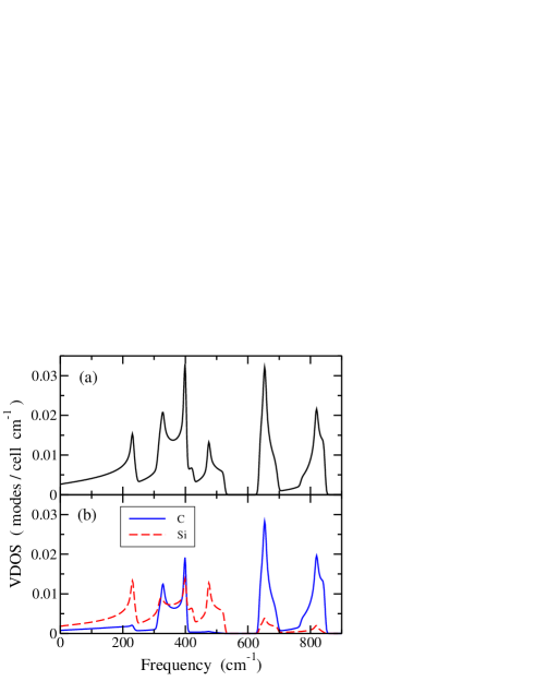
Figure 5: Vibrational density of states of 2D silicon carbide, as derived from the HA for the TB Hamiltonian employed for the PIMD simulations. (a) Total density of states, $g(\omega)$. (b) Solid and dashed curves indicate the VDOS corresponding to carbon, $g_{\rm C}(\omega)$, and silicon, $g_{\rm Si}(\omega)$, respectively.

For comparison with results of our PIMD simulations, it is interesting to obtain the vibrational density of states (VDOS) for the whole Brillouin zone. This has been done by numerical integration over the hexagonal zone, according to the procedure described in Ref. Ramírez and Böhm (1986). In Fig. 5(a) we present the resulting VDOS for 2D SiC, and in Fig. 5(b) we have plotted separately the contributions of carbon (solid curve) and silicon (dashed curve). We will call these contributions $g_{\rm C}(\omega)$ and $g_{\rm Si}(\omega)$, respectively, and their sum yields the total VDOS, $g(\omega)$. Note that the density of states converges to a positive value for $\omega\to 0$, due to the contribution of flexural ZA modes (see below).

In a quantum HA, the vibrational energy per atom in a SiC monolayer is given by

$$E_{\rm vib}=\frac{1}{2N}\sum_{r,\bf k}\hbar\,\omega_{r}({\bf k})\coth\left(\frac{1}{2}\beta\hbar\,\omega_{r}({\bf k})\right)\,,$$ (4)

where the index $r$ ($r$ = 1, …, 6) indicates the phonon bands. The sum in ${\bf k}$ runs over wavevectors ${\bf k}=(k_{x},k_{y})$ in the 2D hexagonal Brillouin zone, with ${\bf k}$ points spaced by $\Delta k_{x}=2\pi/L_{x}$ and $\Delta k_{y}=2\pi/L_{y}$ Herrero and Ramírez (2016); Ramírez and Herrero (2019). In the sequel, $k$ will stand for the wavenumber, i.e., $k=|{\bf k}|$.

Given a VDOS $g(\omega)$ for the lattice modes, the vibrational energy in a continuous approximation is given by

$$E_{\rm vib}=\frac{1}{2}\int_{0}^{\omega_{m}}\hbar\,\omega\coth\left(\frac{1}{2}\beta\hbar\,\omega\right)g(\omega)d\omega\,,$$ (5)

where $\omega_{m}$ is the maximum frequency in the solid. The normalization condition is

$$\int_{0}^{\omega_{m}}g(\omega)d\omega=6,$$ (6)

for the six degrees of freedom in a crystallographic unit cell (one C and one Si).

To analyze the temperature dependence of the energy at low $T$, one can consider the continuous model for frequencies and wavevectors, as in the Debye model for vibrations in solids Ashcroft and Mermin (1976); Kittel (1996). Calling $E_{0}$ the minimum energy of the 2D material, the vibrational energy, $E-E_{0}$, is controlled at low-temperatures by acoustic modes with small $k$, close to the $\Gamma$ point. In our case of 2D SiC, they are TA and LA modes with $\omega_{r}\propto k$, as well as ZA flexural modes with $\omega_{r}\propto k^{2}$.

In general, for a phonon branch $r$ with dispersion relation $\omega_{r}\propto k^{n}$ for small $k$, the contribution to the energy at low $T$ is

$$E_{r}-E_{r}^{0}=\int_{0}^{k_{m}}\frac{\hbar\,\omega_{r}(k)}{\exp[\beta\,\hbar\,\omega_{r}(k)]-1}\,g(k)\,dk\,,$$ (7)

where $k_{m}$ is the maximum wavenumber $k_{m}=(2\pi/A_{0})^{1/2}$ and $g(k)=A_{0}k/2\pi$ for 2D materials. The dispersion relation $\omega_{r}(k)$, yields a vibrational density of states $\bar{g_{r}(\omega)}=g(k)dk/d\omega\sim\omega^{\frac{2}{n}-1}$. Putting $x=\beta\hbar\,\omega/2$, one finds

$$E_{r}-E_{r}^{0}=K\left(\frac{k_{B}T}{\hbar}\right)^{1+\frac{2}{n}}\int_{0}^{x_{m}}x^{\frac{2}{n}}\,({\rm e}^{x}-1)^{-1}\,dx\,,$$ (8)

$K$ being a constant. At low temperatures ($k_{B}T\ll\hbar\,\omega_{m}$, i.e. $x_{m}\gg 1$), we have $E_{r}-E_{r}^{0}\sim T^{1+2/n}$, which means a quadratic dependence of $E_{r}-E_{r}^{0}$ on $T$ for the flexural ZA branch ($n=2$), while $E_{r}-E_{r}^{0}\sim T^{3}$ for LA and TA bands ($n=1$). Considering the constants in the integrals above, we obtain for the ZA phonon branch

$$E_{ZA}(T)=E_{ZA}^{0}+\frac{\pi A_{0}}{24\hbar}\left(\frac{\rho}{\kappa}\right)^{\frac{1}{2}}k_{B}^{2}\,T^{2}\,,$$ (9)

and for LA and TA modes:

$$E_{ac}(T)=E_{ac}^{0}+\frac{\zeta(3)A_{0}}{\pi\hbar^{2}v^{2}}\,k_{B}^{3}\,T^{3}\,,$$ (10)

where $v$ is the sound velocity in each phonon band, and $\zeta$ is Riemann’s zeta function. This gives for the coefficients of $T^{2}$ and $T^{3}$ in the low-temperature expansion of the energy, the values $1.3\times 10^{-7}$ eV/K² and $4.4\times 10^{-10}$ eV/K³, respectively.

IV Energy

Here we present and discuss results of the internal energy of 2D SiC, derived from our simulations in the isothermal-isobaric ensemble for vanishing external stress. At $T=0$, we find a flat SiC sheet for the minimum-energy configuration in a classical calculation with the atoms fixed at their equilibrium positions, yielding an energy $E_{0}=-41.0534$ eV/atom, which is taken as a reference for our calculations at finite temperatures. For a quantum description of the atomic nuclei, one has zero-point in-plane and out-of-plane atomic fluctuations, so that the SiC layer is not totally flat.

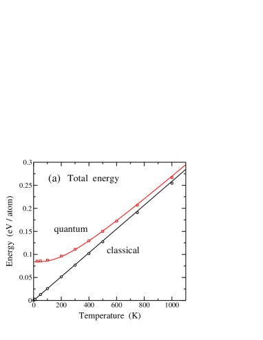
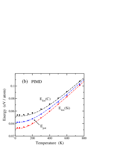
Figure 6: Temperature dependence of the energy per atom in 2D SiC, as derived from the HA (curves) and simulations (symbols). (a) Total energy: circles, classical MD; squares, PIMD. (b) Different contributions to the total energy: potential energy (diamonds); kinetic energy of carbon (circles) and silicon (squares). Error bars are less than the symbol size.

In Fig. 6(a) we display the internal energy of 2D SiC as a function of temperature, obtained from our PIMD simulations (open squares). For comparison, we also present the internal energy found in classical MD simulations (open circles). Solid curves indicate the energy obtained in a HA for both quantum and classical models. In the quantum case, $E-E_{0}$ has been calculated by using Eq. (5) with the VDOS shown in Fig. 5. The open circles are located near the classical harmonic model, i.e., $E^{\rm cl}-E_{0}=3k_{B}T$ per atom. In fact, at low $T$, they are indistinguishable from the harmonic classical energy. For $T\gtrsim 400$ K, the simulation results depart progressively (but slightly) from the harmonic expectancy, and at temperatures in the order of 1000 K this departure is of about a 2%. For the quantum results, however, the energy derived from PIMD simulations is slightly higher than that corresponding to the HA at low temperature, and for increasing $T$ it approaches the result of classical simulations. At $T=1000$ K, we observe a difference of 12 meV/atom between quantum and classical data. For a classical model, at low temperature the atomic motion does not explore the energy regions far from the absolute minimum, due to the smallness of the vibrational amplitudes. For a quantum model, however, the vibrational amplitudes in the limit $T\to 0$ remain finite, and detect anharmonicities in the interatomic potential.

The potential ($E_{\rm pot}$) and kinetic ($E_{\rm kin}$) parts of the internal energy $E$ are given separately in PIMD simulations Herman et al. (1982); Tuckerman (2010); Herrero and Ramírez (2014). For our calculations with external stress $\tau=0$, one has $E-E_{0}=E_{\rm kin}+E_{\rm pot}$. In Fig. 6(b), we show the kinetic and potential energy obtained from PIMD simulations as a function of temperature: $E_{\rm kin}$(Si) (squares); $E_{\rm kin}$(C) (circles), and $E_{\rm pot}$ (diamonds). Dashed curves correspond to the results of a HA, using Eq. (5). In a harmonic model for the vibrational modes, one has $E_{\rm kin}=E_{\rm pot}$ (virial theorem Landau and Lifshitz (1980); Feynman (1972)) for both classical and quantum approaches. From our results, it is plain that anharmonicity produces an increase in the kinetic energy of both C and Si at low temperature, while the potential energy follows closely the harmonic expectation.

For $T\to 0$, we find in the HA $E_{\rm kin}^{0}$(Si) = 31.9 meV and $E_{\rm kin}^{0}$(C) = 51.8 meV. The anharmonic shift amounts to 1.2 and 1.9 meV/atom for Si and C, which represents an increase of 3.8 and 3.7%, respectively, as compared to the harmonic calculation. The slight difference between these relative values is smaller than the uncertainty derived from the error bars of the kinetic energy obtained in our simulations. For the potential energy we obtain $E_{\rm pot}^{0}$ = 41.8 meV / atom. We note that $E_{\rm pot}$ cannot be split into C and Si contributions, as can be done for the kinetic energy. The structure of the TB Hamiltonian does not allow identification of separate contributions to the potential energy for each species. We observe that $E_{\rm pot}$ derived from PIMD simulations gradually deviates from the harmonic expectancy as temperature rises. On the other side, $E_{\rm kin}$ from the simulations approaches the harmonic result for both C and Si for increasing $T$, as the low-temperature shift is compensated for by a slower increase at finite temperatures.

To understand the energy results of PIMD simulations at low $T$, we note that analysis based on perturbation theory and quasiharmonic approximations point out that the low-$T$ energy shift relative to a harmonic model is basically caused by a change of the kinetic energy Herrero and Ramírez (2016); Brito et al. (2019). This happens, indeed, for perturbed harmonic oscillators at $T=0$ (considering perturbations of $x^{3}$ or $x^{4}$ type), where first-order energy changes are due to shifts in $E_{\rm kin}$, while $E_{\rm pot}$ stays unmodified respect to the harmonic energy Landau and Lifshitz (1965).

V Interatomic distances

In this section we discuss the interatomic distance $d_{\rm Si-C}$ between nearest neighbors in 2D SiC. Zero-point motion is expected to cause an increase in the equilibrium $d_{\rm Si-C}$. This is a combination of quantum dynamics on one side and anharmonicity of the lattice vibrations on the other. For purely harmonic quantum vibrations, no change in $d_{\rm Si-C}$ can appear.

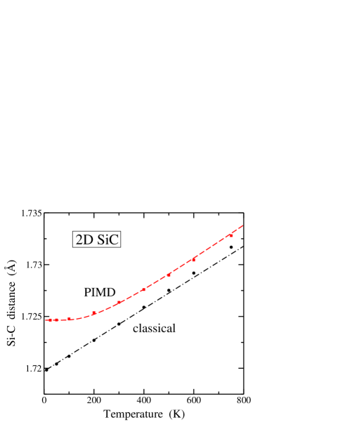
Figure 7: Temperature dependence of mean interatomic distance, $d_{\rm Si-C}$ in 2D silicon carbide. Solid circles and squares represent results of classical and PIMD simulations, respectively. Error bars are less than the symbol size. The dashed curve is a fit of the quantum results to Eq. (11). The dashed-dotted line is a linear fit of the classical MD results for $T<500$ K.

In Fig. 7 we display the mean Si–C distance as a function of temperature. Solid squares represent results of PIMD simulations, whereas circles are data points obtained from classical MD simulations. At low temperature ($T\to 0$), we obtain in the quantum simulations an interatomic distance of 1.725 Å, which increases for rising temperature. Comparing results for $N$ = 112 and 216 atoms, we find that size effects of the finite simulation cells on $d_{\rm Si-C}$ are negligible, as in fact they are smaller than the error bars of the simulation results (less than the symbol size in Fig. 7). For comparison with the results of 2D SiC, we note that PIMD simulations of 3C SiC employing the same TB Hamiltonian give a zero-temperature distance $d_{\rm Si-C}$ = 1.888 Å, somewhat larger than in the 2D sheet Ramírez et al. (2008); Herrero et al. (2009).

At low $T$, the results of classical simulations display a linear increase with rising temperature, as shown in Fig. 7. This is typical for interatomic distances in solids from classical calculations Kittel (1996). For $d_{\rm Si-C}$ in 2D SiC we find in the low-temperature classical limit a value of 1.720 Å. The dashed-dotted line in Fig. 7 is a linear fit to the classical results for $T<500$ K. We observe that the results of the MD simulations depart progressively from this line at higher temperatures.

Comparing the low-temperature results for PIMD and classical MD simulations, we find a zero-point expansion $\Lambda_{0}=5\times 10^{-3}$ Å due to quantum fluctuations, i.e., an increase in $d_{\rm Si-C}$ of a 0.3% with respect to the classical value. Note that such an increase in bond length associated to nuclear quantum effects turns out to be much larger than the precision attained for interatomic distances from diffraction experiments Yamanaka et al. (1994); Ramdas et al. (1993); Kazimorov et al. (1998). The zero-point bond dilation is similar in magnitude to the thermal expansion obtained in the classical simulations from $T=0$ to 350 K. The difference between quantum and classical results decreases as temperature is raised, since they converge to one another at high $T$, when the relevance of quantum fluctuations decreases. At $T=750$ K, this difference is still observable in Fig. 7, but it is about 5 times smaller than the zero-point bond expansion. For the interatomic distance in monolayer graphene, a TB Hamiltonian analogous to that employed here gives a zero-point bond expansion of a 0.5%, i.e., a relative increase larger than for the larger Si–C bond in 2D silicon carbide.

Both thermal bond expansion and zero-point dilation are related to anharmonicity in the interatomic potential, as in 3D crystalline materials. For 2D SiC, these effects are mainly associated to anharmonicity of the stretching vibrations of the Si–C bonds. Something more complex is needed to describe thermal changes of the in-plane area $A_{p}$, because of the coupling between out-of-plane and in-plane vibrational modes, as discussed below.

A simple quantitative approach to the temperature dependence of the Si–C bond length can be obtained in the spirit of a quasiharmonic approximation Herrero and Ramirez (2021b). In this approach one can write

$$d_{Q}(T)=d_{0}+\frac{\Lambda_{0}}{E_{Q}(\omega_{\rm eff},0)}E_{Q}(\omega_{\rm eff},T)\,,$$ (11)

where $\Lambda_{0}$ is the zero-point quantum expansion, $\omega_{\rm eff}$ is an effective frequency, and $E_{Q}$ is the harmonic vibrational energy for $\omega_{\rm eff}$. In the context of such quasiharmonic approximation, $\Lambda_{0}$ can be interpreted as a ratio $\gamma_{\rm eff}/B_{\rm eff}$ between a Grüneisen parameter and an effective compression modulus $B_{\rm eff}$ Herrero and Ramirez (2021b). The dashed curve in Fig. 7 shows the interatomic distance obtained using Eq. (11) with an effective frequency $\omega_{\rm eff}$ = 405 cm^-1, which follows closely the results of PIMD simulations in the displayed temperature range.

VI Atomic mean-square displacements

The PIMD simulations employed here are well-suited to study atomic delocalization in 3D space at finite temperatures. This contains both, a classical (thermal) delocalization, as well as a contribution due to the quantum character of atomic nuclei. The former is measured by the motion of the center-of-gravity (centroid) of the ring polymers associated to the quantum particles, and the latter is given by extension of the quantum paths (MSD of the beads with respect to their centroid).

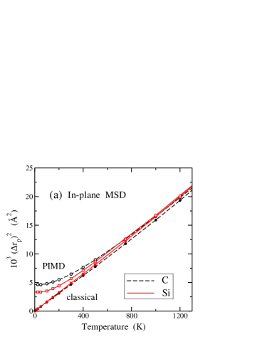
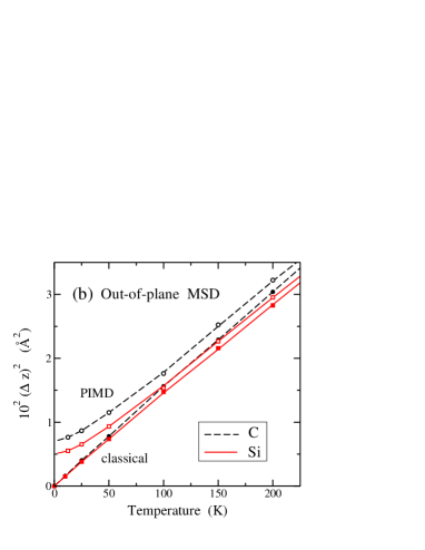
Figure 8: Atomic mean-square displacements in 2D silicon carbide. (a) In-plane MSD, $(\Delta r_{p})^{2}$, for carbon (circles) and silicon (squares) as a function of temperature. Solid and open symbols indicate results of classical MD and PIMD simulations, respectively. (b) Out-of-plane MSD, $(\Delta z)^{2}$. Symbols and curves have the same meaning as in (a). Error bars are in the order of the symbol size. Curves are guides to the eye.

We will present separately the in-plane and out-of-plane atomic MSDs. In Fig. 8(a) we display the MSD of C and Si atoms on the $(x,y)$ plane. Symbols are data points obtained from our simulations: open and solid symbols indicate results of PIMD and classical MD simulations, respectively. Circles and dashed curves correspond to carbon, whereas squares and solid curves represent data for silicon. We have checked that contributions along the $x$ and $y$ directions are indistinguishable within the error bars of our simulation results (in the order of the symbol size). The quantum results converge for $T\to 0$ to $(\Delta r_{p})_{0}^{2}=(\Delta x)_{0}^{2}+(\Delta y)_{0}^{2}$ = $4.7\times 10^{-3}$Ų and $3.4\times 10^{-3}$ Ų for C and Si, respectively. For the quantum data, we find $(\Delta r_{p})^{2}_{\rm C}$ $>(\Delta r_{p})^{2}_{\rm Si}$ in the whole temperature range displayed in Fig. 8(a), and the opposite happens for the classical results.

In a classical calculation the atomic MSDs do not depend on the atomic mass, but they indeed change with the interatomic potential felt by the atomic nuclei. In our case, the effective potential felt by Si atoms is somewhat softer than that felt by C atoms, which causes a larger classical MSD for Si (solid curve) than for C atoms (dashed curve). This effect does also appear in the quantum results, but in this case it is overwhelmed by the influence of the atomic mass, i.e., at low temperature the contribution of a mode with frequency $\omega$ contribute to the MSD of an atom with mass $M$ as $\sim\hbar/2M\omega$. At high $T$ classical and quantum results converge one to the other for each atomic species. This means that the quantum MSD in the $(x,y)$ plane for C and Si cross at a certain temperature higher than 600 K. In fact, this happens at $T\approx 800$ K (not shown in Fig. 8(a)).

The atomic motion in the out-of-plane $z$ direction is important for various properties of 2D materials, since it is the origin of bending in their sheets. In Fig. 8(b) we display results for the MSD of C and Si in the $z$-direction, obtained from PIMD and classical MD simulations. Symbols and curves have the same meaning as in Fig. 8(a). Note that values of $(\Delta z)^{2}$ for C and Si are clearly larger than the corresponding ones in the layer plane, due to the contribution of low-frequency flexural modes (ZA) close to the $\Gamma$ point.

For the quantum results in the low-$T$ limit, we find $(\Delta z)_{0}^{2}=7.2\times 10^{-3}$ Å² and $5.1\times 10^{-3}$ Å², for C and Si respectively. The ratio between these values is close to the inverse square root of the mass ratio, i.e., $(\Delta z)_{\rm C}^{2}/(\Delta z)_{\rm Si}^{2}$ $\approx(M_{\rm Si}/M_{\rm C})^{1/2}$. For the out-of-plane motion, the classical MSD for C is somewhat higher than that of Si, contrary to the findings for in-plane MSDs shown above. This is related to details of the effective potential felt by each atomic species, which shows different behavior in out-of-plane and in-plane directions.

From earlier simulations of graphene and other 2D materials Herrero and Ramírez (2016) it is known that, although atomic MSDs in the layer plane are rather insensitive to the system size, out-of-plane MSD have a size effect, in particular at high temperatures. This is due to the presence of long-wavelength vibrational modes with low frequency and large vibrational amplitudes in the ZA flexural band. This phonon branch may be described at finite temperatures by a dispersion relation of the form $\rho\,\omega({\bf k})^{2}=\sigma k^{2}+\kappa k^{4}$, where $\sigma$ is an effective stress Herrero and Ramírez (2016); Ramírez and Herrero (2019). For our present purposes, $\sigma$ is negligible and the ZA branch can be considered as parabolic: $\omega({\bf k})\approx\sqrt{\kappa/\rho}\,k^{2}$ with $\kappa$ = 1.0 eV. Vibrational modes with longer wavelength $\lambda$ appear for increasing system size $N$. This means that one has an effective cut-off $\lambda_{max}\approx L$, where $L=(NA_{p})^{1/2}$. Then, we have $k_{min}=2\pi/\lambda_{max}$, so that $k_{min}\sim N^{-1/2}$, which yields a frequency $\omega_{min}\sim N^{-1}$. From the contributions of the whole bands, $(\Delta z)^{2}$ for a given atomic species scales as $N^{\eta}$, with an exponent $\eta>0$. A precise estimation of $\eta$ for 2D SiC would require carrying out longer simulations (millions of simulation steps) with cell sizes much larger than those considered here. Our present procedure with a TB Hamiltonian does not allow us to perform such simulations for $N\gtrsim 400$ atoms in moderately long computing times. We also note that the relative statistical uncertainty (error bar) derived from PIMD simulations depends on the physical variable at hand, and it is in particular relatively large for the in-plane area $A_{p}$.

The consistency of the results of our quantum simulations in the coordinate and momentum space can be checked from the atomic MSDs and kinetic energy given above. In general, for a particle described by quantum mechanics, the RMS displacements of the coordinate $x$ and momentum $p_{x}$ have to comply with the Heisenberg’s uncertainty relation $\Delta x\,\Delta p_{x}\geq\hbar/2$ (see, e.g., Ref. Cohen-Tannoudji et al. (1977)), so that

$$(\Delta p_{x})^{2}\geq\frac{\hbar^{2}}{4(\Delta x)^{2}}\,.$$ (12)

and similar expressions apply for $y$ and $z$ coordinates. For the atomic nuclei considered here, we have $\langle p_{x}\rangle=0$, so that $(\Delta p_{x})^{2}=\langle p_{x}^{2}\rangle$, and the kinetic energy of a particle with mass $M$ can be written as

$$E_{\rm kin}=\frac{\langle{\bf p}^{2}\rangle}{2M}=\frac{1}{2M}\left[(\Delta p_{x})^{2}+(\Delta p_{y})^{2}+(\Delta p_{z})^{2}\right]\,.$$ (13)

Then, using Eqs. (12) and (13), we find

$$E_{\rm kin}\geq F\equiv\frac{\hbar^{2}}{8M}\left[(\Delta x)^{-2}+(\Delta y)^{-2}+(\Delta z)^{-2}\right]\,.$$ (14)

where $F$ is a function of the atomic MSDs. Thus, one has a lower bound for the kinetic energy of the particle, defined from its delocalization in real space.

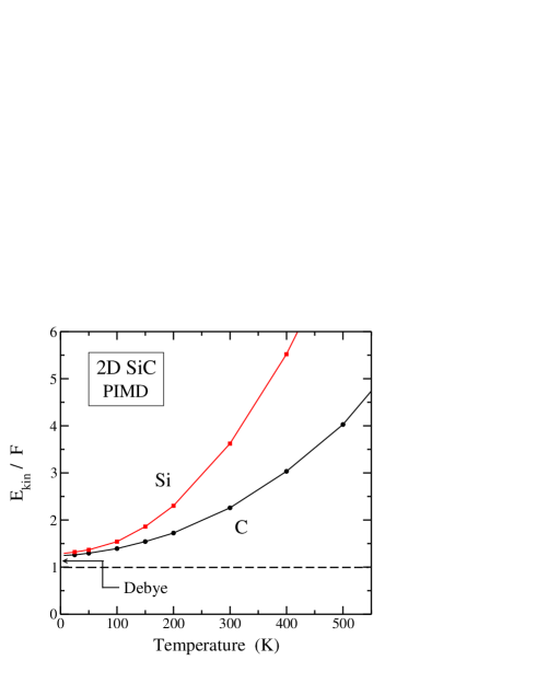
Figure 9: Temperature dependence of the ratio $E_{\rm kin}/F$ between the kinetic energy and the function $F$ defined in Eq. (14). Symbols represents results derived from PIMD simulations for carbon (circles) and silicon (squares). Solid curves are guides to the eye. An arrow indicates the value expected in a Debye approximation for the vibrational modes.

In Fig. 9 we present the ratio $E_{\rm kin}/F$ as a function of temperature for carbon (circles) and silicon (squares), as derived from our PIMD simulations of 2D SiC. The dashed line indicates the lower bound allowed by the uncertainty relations, i.e., $E_{\rm kin}/F=1$. For the sake of comparison, we note that for an isotropic 3D harmonic oscillator with frequency $\omega$, the MSD in each direction ($x$, $y$, and $z$) for the ground state is $\hbar/2M\omega$, and the kinetic energy $(E_{\rm kin})_{0}=3\hbar\,\omega/4$ Cohen-Tannoudji et al. (1977). This means that the ratio $E_{\rm kin}/F$ converges to unity in the limit $T\to 0$. For atomic motion in condensed matter, one has a frequency dispersion, which can be represented by an isotropic 3D Debye model Kittel (1996); Ashcroft and Mermin (1976), with a vibrational density of states $\mu(\omega)\propto\omega^{2}$ and a high-frequency cutoff $\omega_{D}$. In this case, considering harmonic vibrations, one finds for $T\to 0$ a ratio $E_{\rm kin}/F=1.125$, somewhat higher than for a single harmonic oscillator Herrero and Ramírez (2020). This value for the Debye model is indicated in Fig. 9 by an arrow, a little below the results of our simulation for carbon and silicon in anisotropic 2D SiC.

VII In-plane vs real area

In our simulations in the isothermal-isobaric ensemble, one fixes $N$, $T$, and the applied 2D stress in the $(x,y)$ plane (here, $\tau=0$), permitting changes in the area $A_{p}$ of the simulation cell. This area is a practical variable to perform atomistic simulations of 2D materials, and has been studied before in various works as a function of temperature and external stress Gao and Huang (2014); Brito et al. (2015); Zakharchenko et al. (2009); Los et al. (2016). It is not, however, a variable to which one can attribute properties of a real material surface, but a projected area on the reference $(x,y)$ plane. In our case, Si and C atoms can move out-of-plane in the $z$ direction, and measuring the real surface of the SiC layer will give values larger than the in-plane area of the 2D simulation cell.

Then, it is interesting to deal with an additional surface defined from the atomic positions along a simulation run. We consider a real surface $A$ in 3D space for 2D SiC, obtained from the actual geometry of the layer Herrero and Ramírez (2018). This area $A$ is calculated by a triangulation defined from the actual atomic positions along the simulations. The contribution of each structural hexagon is obtained as a sum of six triangular areas. Each triangle is built up from the coordinates of neighboring Si and C atoms and the center (mean position) of the hexagon Ramírez and Herrero (2017). One can use other definitions for a real area, as those based on interatomic distances, which yield results similar to that considered here Hahn et al. (2016); Herrero and Ramírez (2016).

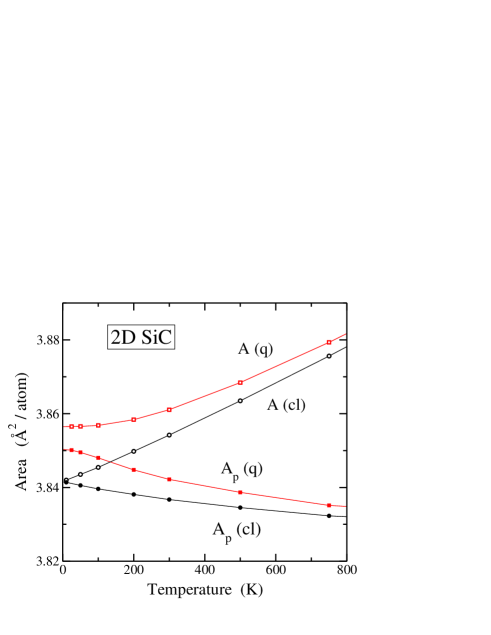
Figure 10: In-plane area, $A_{p}$ (solid symbols), and real area per atom, $A$ (open symbols), vs the temperature. Circles and squares correspond to classical MD and PIMD simulations, respectively. The labels “q” and “cl” refer to quantum and classical areas. Error bars are smaller than the symbol size. Curves are guides to the eye.

In Fig. 10 we present the temperature dependence of the areas $A$ and $A_{p}$. In both cases, we show results from PIMD (squares) and classical simulations (circles). Solid and open symbols correspond to the areas $A$ and $A_{p}$, respectively. In the classical limit, the surfaces $A_{p}$ and $A$ take the same value for $T\to 0$, since the real surface becomes planar with vanishing out-of-plane atomic displacements. This area corresponds to the minimum-energy configuration, $A_{0}=3.8415$ Å²/atom. In the quantum results, however, $A_{p}$ and $A$ do not converge to the same low-temperature limit. In fact, for $T\to 0$, $A$ is larger than $A_{p}$ by $6\times 10^{-3}$ Ų/atom. Such a difference in the low-$T$ limit appears because the SiC sheet is not totally planar, because of the zero-point motion in the $z$ direction.

Apart from differences in the low-temperature behavior, a clear feature distinguishing $A_{p}$ and $A$ is their behavior as a function of temperature. One observes first that the surface $A$ is larger than $A_{p}$, and the difference between both rises as temperature increases. This is consistent with the fact that $A_{p}$ is a projection of $A$ on the $(x,y)$ plane, and the real surface becomes progressively bent as temperature rises and atomic motion in the $z$ direction becomes more relevant. The in-plane area $A_{p}$ is found to decrease for increasing $T$ ($dA_{p}/dT<0$) in both classical and quantum simulations. $A_{p}$ reaches a minimum for $T\approx 1400$ K (not shown in Fig 10), and slowly increases at higher temperature, similarly to the results found for graphene Herrero and Ramírez (2016). For the real area $A$, however, we find $dA/dT>0$ in the whole temperature range considered here, for both classical and PIMD simulations. Note that the temperature derivative of $A$ and $A_{p}$ converges to zero in the low-$T$ limit, as required by the third law of thermodynamics.

To explain the temperature dependence of the in-plane area $A_{p}$, we observe that it is governed by two main factors. First, the real area rises for increasing $T$, which is associated with an increase of its projection on the $(x,y)$ plane, i.e. the area $A_{p}$. Second, bending or rippling of the SiC layer gives rise to a lowering of the in-plane area. The second factor dominates in the temperature region shown in Fig. 10, causing a decrease in $A_{p}$ for temperatures lower than 1400 K. At high temperatures, the first factor (expansion of $A$) dominates and one has $dA_{p}/dT>0$. This behavior of $A_{p}$ for 2D SiC is similar to that described for graphene Gao and Huang (2014); Michel et al. (2015); Herrero and Ramírez (2016), but for the latter the difference between classical and quantum results is about two times larger than for silicon carbide.

The difference between in-plane and real area has been denoted hidden area for graphene Nicholl et al. (2017) and excess area for fluid membranes Helfrich and Servuss (1984); Fournier and Barbetta (2008). We define, for each temperature $T$, the dimensionless excess area of a crystalline membrane as $\Omega=(A-A_{p})/A_{p}$. In an analytical formulation of membranes in the continuum limit, the relation between $A$ and $A_{p}$ can be written as Imparato (2006); Waheed and Edholm (2009); Ramírez and Herrero (2017)

$$A=\int_{A_{p}}dx\,dy\,\sqrt{1+(\nabla h(x,y))^{2}}\;,$$ (15)

where $h(x,y)$ is the height of the surface, or the distance to the mean $(x,y)$ plane of the sheet. The difference $A-A_{p}$ may be calculated by expanding $h(x,y)$ as a Fourier series with wavevectors ${\bf k}$ in the 2D Brillouin zone Safran (1994); Chacón et al. (2015); Ramírez and Herrero (2017). One obtains

$$A=A_{p}\left[1+\frac{1}{2N}\sum_{\bf k}k^{2}\langle|H({\bf k})|^{2}\rangle\right]\;,$$ (16)

where $H({\bf k})$ are the Fourier components of $h(x,y)$. Thus, the excess area can be written as

$$\Omega=\frac{1}{2N}\sum_{r,{\bf k}}k^{2}\langle|\xi_{r}({\bf k})|^{2}\rangle\;,$$ (17)

where the sum in $r$ is extended to vibrational modes with $z$ polarization, i.e., ZA and ZO, and $\xi_{r}({\bf k})$ are the vibrational amplitudes in branch $r$. The contribution of ZO modes is negligible vs. that of low-frequency ZA modes for ${\bf k}$ close to the $\Gamma$ point (small $k$).

In a harmonic approximation, the contribution of C atoms to $\langle|\xi_{\rm ZA}({\bf k})|^{2}\rangle$ is given by

$$\langle|\xi_{\rm ZA}^{\rm C}({\bf k})|^{2}\rangle=\frac{\hbar}{2M_{\rm C}\,\omega_{\rm ZA}({\bf k})}\coth\left[\frac{1}{2}\beta\hbar\,\omega_{\rm ZA}({\bf k})\right]\;,$$ (18)

and similarly for the Si contribution. Putting $\omega_{\rm ZA}=\sqrt{\kappa/\rho}\,k^{2}$, and using the continuous approximation for wavenumbers as in Sec. III for the vibrational energy, we have for the low-$T$ limit of the excess area:

$$\Omega_{0}=\frac{\hbar}{4}\left(\frac{\rho}{\kappa}\right)^{\frac{1}{2}}\int_{0}^{\omega_{m}}\left[\frac{g_{\rm ZA}^{\rm C}(\omega)}{M_{\rm C}}+\frac{g_{\rm ZA}^{\rm Si}(\omega)}{M_{\rm Si}}\right]d\omega\,.$$ (19)

Introducing into this expression the VDOS corresponding to the ZA branch for C and Si, we find a value $\Omega_{0}=1.6\times 10^{-3}$, which coincides with that obtained for the areas $A$ and $A_{p}$ from PIMD at low temperature (see Fig. 10). At high temperature, the excess area can be approximated by the classical limit in Eq. (17), where the contribution of atoms with mass $M$ to $\langle|\xi_{\rm ZA}({\bf k})|^{2}\rangle$ is given by $k_{B}T/M[\omega_{\rm ZA}({\bf k})]^{2}$. This yields a linear increase in $\Omega$ as a function of temperature for high $T$. In this classical limit, $\Omega$ vanishes for $T\to 0$.

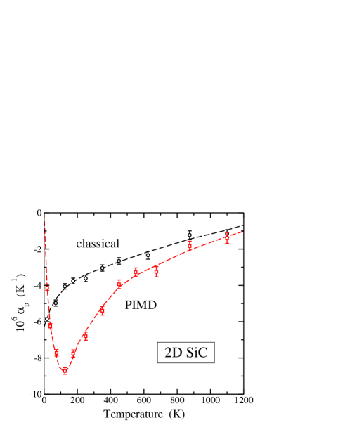
Figure 11: In-plane thermal expansion coefficient $\alpha_{p}$ vs temperature, as derived from classical (circles) and PIMD simulations (squares) of 2D silicon carbide. Symbols are data points obtained from numerical derivatives of the in-plane area $A_{p}$. Curves are guides to the eye.

In connection with the area $A_{p}$, one can define an in-plane thermal expansion coefficient (TEC) as

$$\alpha_{p}=\frac{1}{A_{p}}\left(\frac{\partial A_{p}}{\partial T}\right)_{\tau}\,.$$ (20)

This TEC has been studied earlier for 2D materials, and in particular for graphene Herrero and Ramírez (2018); Jiang et al. (2009); Yoon et al. (2011); Bao et al. (2009). In Fig. 11 we present $\alpha_{p}$ calculated from our simulation results for 2D SiC up to $T$ = 1200 K. Open squares are data points found from a numerical derivative of the area $A_{p}$ obtained in PIMD simulations. For comparison we also show results for $\alpha_{p}$ derived from classical MD simulations (open circles). The quantum results display a minimum of $-8.7\times 10^{-6}$ K^-1 at a temperature $T_{m}\approx 130$ K. At higher $T$, $\alpha_{p}$ decreases in absolute value and eventually reaches zero for $T\sim$ 1400 K. At low $T$, $\alpha_{p}$ approaches zero, as required by the third law of thermodynamics. The value of the minimum $\alpha_{p}$ for SiC is close to the result reported earlier for graphene: $-9.2\times 10^{-6}$ K^-1, whereas $T_{m}$ for the former is somewhat lower than for the latter ($\approx 200$ K).

We note that the results for $\alpha_{p}$ derived from classical simulations approach to the quantum data at high $T$, but clearly depart from the PIMD results at low temperature. In fact, the classical TEC converges to $-6\times 10^{-6}$ K^-1 for $T\to 0$, and does not vanish in this limit, which is a well-known limitation of classical models at low temperature.

One can also define a TEC $\alpha=(\partial A/\partial T)/A$ for the real area $A$ of 2D SiC. The real area behaves as a function of $T$ in a similar fashion to the crystal volume of most 3D solids Ashcroft and Mermin (1976), i.e., it increases at all finite temperatures. Then, the TEC $\alpha$ is positive for all temperatures, as shown earlier for graphene Herrero and Ramírez (2018).

VIII Summary

In this paper, we have presented and discussed results of PIMD simulations of 2D silicon carbide in the isothermal-isobaric ensemble ($N\tau T$) in a temperature range from 25 to 1500 K. The dynamics of this layered material displays typical characteristic of membranes, and an atomic-scale analysis has given us insight into the relation between its vibrational modes with structural and thermal properties at finite temperatures. The main focus of our research has been an assessment of nuclear quantum effects, which can be made by a comparison of the quantum results with those obtained from classical MD simulations.

The use of a TB Hamiltonian to describe the interatomic interactions along with PIMD simulations to take into account the nuclear quantum delocalization has allowed us to study 2D silicon carbide, with relatively light constituent atoms. Our findings show that explicitly taking into account the quantum character of atomic nuclei gives appreciable corrections to the classical results, especially at low temperatures, where classical simulations fail to yield the correct behavior of physical observables, required by the third law of thermodynamics. For $T$ near room temperature, nuclear quantum effects are still nonnegligible.

The interatomic distance $d_{\rm Si-C}$ and the in-plane area expand with respect to the classical expectation, which is a joint signature of zero-point motion and anharmonicity of the interatomic potential. For $T\to 0$, the mean Si–C bond and $A_{p}$ grow by about a 0.3%. The thermal expansion of the in-plane area derived from PIMD simulations turns out to be negative for $T\lesssim$ 1400 K, and positive for higher $T$. The thermal contraction of $A_{p}$, i.e. $\alpha_{p}<0$, is caused by an increasing amplitude of out-of-plane vibrations (mainly ZA modes) as temperature is raised. The real area $A$, however, has a positive thermal expansion, $\partial A/\partial T>0$, in the whole temperature range considered here, and the difference $A-A_{p}$ grows for rising $T$.

We have quantified the anharmonicity of the vibrational modes by comparing results derived from a pure harmonic approximation (VDOS in Fig. 5) with those given by PIMD simulations. An additional assessment of anharmonicity is obtained from the difference between the total kinetic and potential energy of the system found in the simulations, since they should coincide for harmonic vibrations. At low $T$, we obtain for the kinetic energy of both C and Si an anharmonic shift of 4% with respect to the HA , whereas the potential energy of the layer is not affected by anharmonicity (as in first-order perturbation theory).

We have found for the bending constant $\kappa$ of 2D SiC a value of 1.0 eV, smaller than that corresponding to graphene ($\kappa$ = 1.5 eV), indicating a larger flexibility of the former to bend and ripple at finite temperatures. For the 2D modulus of hydrostatic compression we have found $B_{xy}$ = 5.5 eV/Ų for SiC vs 12.7 eV/Ų for graphene, indicating a larger rigidity of the latter in the layer plane. It will be interesting to research how these constants evolve from one material to the other, by studying 2D Si_xC_1-x in a wide composition range, as well as to consider their changes due to nuclear quantum motion.

Finally, we note that PIMD simulations in the isothermal-isobaric ensemble for tensile and compressive stress ($\tau\neq 0$) can give additional information on structural and mechanical properties of 2D SiC layers far from the minimum-energy configuration. This kind of simulations may provide insight into the stability of this material in a stress-temperature phase diagram.

Data availability

The data that support the findings of this study are available from the corresponding author upon reasonable request.

Author contribution statement

Carlos P. Herrero: Data curation, Investigation, Validation, Original draft

Rafael Ramírez: Methodology, Software, Investigation, Validation

Declaration of Competing Interest

The authors declare that they have no known competing financial interests or personal relationships that could have appeared to influence the work reported in this paper.