Abstract

We demonstrate that the Ising model on a general triangular graph with 3 distinct couplings $K_{1},K_{2},K_{3}$ corresponds to an affine transformed conformal field theory (CFT). Full conformal invariance of the $c=1/2$ minimal CFT is restored by introducing a metric on the lattice through the map $\sinh(2K_{i})=\ell^{*}_{i}/\ell_{i}$ which relates critical couplings to the ratio of the dual hexagonal and triangular edge lengths. Applied to a 2d toroidal lattice, this provides an exact lattice formulation in the continuum limit to the Ising CFT as a function of the modular parameter. This example can be viewed as a quantum generalization of the finite element method (FEM) applied to the strong coupling CFT at a Wilson-Fisher IR fixed point and suggests a new approach to conformal field theory on curved manifolds based on a synthesis of simplicial geometry and projective geometry on the tangent planes.

1 Introduction

Ever since Onsager’s famous solution in 1944 [1], the 2d Ising lattice model has continued to stimulate a deeper understanding of critical phenomena and conformal field theory (CFT). On both a uniform square and triangular lattice, the 2d Ising model is equivalent to the $c=1/2$ minimal CFT on $\mathbb{R}^{2}$ at the second order phase point. The discrete translations and the 4-fold and 6-fold discrete rotations (for the square and triangular lattice, respectively) are sufficient to guarantee the restoration of Poincaré invariance (1 rotation and 2 translations). Combined with scale invariance at a second order fixed point, this apparently implies full conformal symmetry in the continuum limit [2].

Here we consider the more general triangular Ising lattice model partition function,

$$Z=\sum_{s_{n}=\pm 1}e^{\;\textstyle K_{1}s_{n}s_{n+\hat{1}}+K_{2}s_{n}s_{n+\hat{2}}+K_{3}s_{n}s_{n+\hat{3}}}\;,$$ (1)

with 3 independent couplings ($K_{1},K_{2},K_{3}$) on the links connecting black sites illustrated in Fig. 1.

Figure 1: On the left, the triangular graph (black dots) and its hexagonal dual graph (open circles). On the right, the 3 independent couplings assigned to each triangle.

Now, the map from the lattice to the continuum at a second order phase transition is less obvious. Indeed, even at the second order phase transition, assigning equal lengths to the edges in the graph does not in general restore rotational symmetry. Although the action (1) has discrete translations on three axes, rotational symmetry restricted to $\pi$ and reflections is insufficient to restore full rotational symmetry in the continuum limit except in the special cases of the square ($K_{1}=K_{2},K_{3}=0$) and equilateral triangular ($K_{1}=K_{2}=K_{3}$) lattice. Assuming a uniform lattice on the edges of the triangular graph, in general the geometry that emerges at the critical surface is instead an affine transformation of $\mathbb{R}^{2}$. Affine transformations preserve parallel lines but not angles, and map circles into ellipses. Consistent with these properties, the correlation length contours of an affine-transformed CFT form ellipses. However, in the spirit of the finite element method (FEM), an alternative is to introduce a metric on the graph by assigning unequal lengths $\ell_{1},\ell_{2},\ell_{3}$ in correspondence with the couplings $K_{1},K_{2},K_{3}$. We prove that the identity

$$\sinh(2K_{1})=\ell^{*}_{1}/\ell_{1}\quad,\quad\sinh(2K_{2})=\ell^{*}_{2}/\ell_{2}\quad,\quad\sinh(2K_{3})=\ell^{*}_{3}/\ell_{3}$$ (2)

on the critical surface restores rotational symmetry in the continuum. The dual lengths $\ell^{*}_{i}$ are defined as the lengths of the corresponding links on the hexagonal dual lattice, with dual sites defined to be at the circumcenter of each triangle in the original lattice. While it is dangerous to claim originality for the classic Ising model, we are unaware of this result in the literature. This result is of course consistent with the special cases of the Ising CFT on a uniform square lattice ($\beta_{c}=K_{1}=K_{2},K_{3}=0$) and equilateral triangular lattice ($\beta_{3}=K_{i}$) and the well known critical temperatures: $\beta_{c}=\ln(1+\sqrt{2})$ with $\ell^{*}_{i}/\ell_{i}=1$ and $\beta_{3}=\ln(3)/4$ with $\ell^{*}_{i}/\ell_{i}=1/\sqrt{3}$, respectively.

Interestingly, this strong coupling solution (2) resembles the classic FEM solution based on the discrete exterior calculus (DEC) for a free scalar on a simplicial lattice. Applied to this triangular graph, with action

$$S_{\text{free}}=\frac{1}{2}\sum_{n}[K_{1}(\phi_{n}-\phi_{n+\hat{1}})^{2}+K_{2}(\phi_{n}-\phi_{n+\hat{2}})^{2}+K_{3}(\phi_{n}-\phi_{n+\hat{3}})^{2}]$$ (3)

the DEC prescription to converge to the continuum Laplacian on $\mathbb{R}^{2}$ must satisfy the condition

$$2K_{1}=\ell^{*}_{1}/\ell_{1}\quad,\quad 2K_{2}=\ell^{*}_{2}/\ell_{2}\quad,\quad 2K_{3}=\ell^{*}_{3}/\ell_{3}\;.$$ (4)

Thus, the free scalar 2d CFT is remarkably similar to the strong coupling Ising solution. We note that the FEM represents a very general solution to free conformal field theory (CFT) in any dimension for scalar, fermion, and gauge fields on a properly designed simplicial complex for any smooth Riemann manifold. This is a consequence of the equivalence of pure gaussian field theory to linear partial differential equation or equation of motion. Our so-called quantum finite element (QFE) project  [3, 4, 5] is an attempt to extend the simplicial lattice methods to quantum field theory on general Riemann manifolds – a much more difficult problem even for UV-renormalizable theories due to UV divergence.

In both Eq. 2 and Eq. 4, it is instructive to regard geometry as an emergent property at a second order fixed point. In lattice field theory on regular (hypercubic) graphs, this feature is often subsumed in the analysis of relevant operators at weak coupling at a UV fixed point. Nonetheless, the geometry of a manifold for the quantum field theory is dictated by the dynamics of the fixed point. Not only is this the central concern of the lattice Quantum Finite Element (QFE) project [3, 4, 5] to define quantum field theory on curved Riemann manifolds, but the Regge Calculus [6, 7] approach to gravity also hopes to have space-time geometry emerge at distances far from the Planck scale.

The focus of this paper is to derive the identity in Eq. 2 and to understand if it has implications in a wider context. To this end it appears natural and possibly useful in exploring generalizations to other systems to note how this problem relates to in the language of projective geometry. We begin with a review in Sec. 2 of the fundamental elements at the intersection of projective geometry and FEM discrete exterior algebra calculus. Since the subsequent algebra is self-contained the reader may prefer to skip this section at first.

In Sec. 3 we summarize the star-triangle identity that maps the critical surface of the hexagonal graph to the triangular graph, followed by Sec. 4 where we determine the geometry by matching to a loop expansion of the theory of a free Wilson-Majorana fermion. Interestingly, the formalism depends crucially on the simpler properties of the trivalent form of the hexagonal graph. Finally, in Sec. 5.1 we show that this general projective Ising model allows a direct computation of the general finite torus as a function of the modular parameter, which was anticipated by Nash and O’Conner in Ref. [8]. In Sec. 5.2 we give numerical verification of our projective Ising model on $\mathbb{R}^{2}$ as the limit of a finite toroidal lattice and in Sec. 5.3 we illustrate the advantage of the radial quantization configuration in the cylindrical geometry. We hope that numerical methods may be able to extend this approach to other theories that are not amenable to analytical methods. The conclusion in Sec. 6 suggests how this might be extended to CFT on spheres or cylinders for radial quantization in the QFE program.

2 Motivation and Geometric Background

We first encountered the affine projection in the QFE project when constructing a simplicial triangulation [4] of the sphere $S^{2}$. As illustrated in Fig. 2, a natural approach to a smooth simplicial triangulation was to first refine the twenty flat faces of an icosahedron with equilateral triangles and then project each vertex radially outward onto a sphere of radius $R$, as illustrated in Fig. 2. One advantage was that this preserved exactly the icosahedral subgroup of $O(3)$.

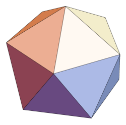
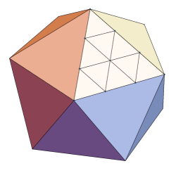
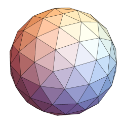
Figure 2: The $L$-th level of refinement of the icosahedron subdivides triangles into $L^{2}$ smaller triangles for a total of $N_{\triangle}=20L^{2}$ faces, $E=30L^{2}$ edges and $N=2+10L^{2}$ sites. Illustrated on the left the icosahedron, followed by the $L=3$ refinement with $2+10L^{2}=92$ vertices and finally on the right subsequently projected onto the unit sphere.

From the perspective point at the center of the sphere, as illustrated in Fig. 3, in this construction each equilateral triangle undergoes an affine transformation to the tangent plane. In the continuum limit of infinitesimal triangles with edge length $\ell_{i}\sim a\rightarrow 0$ (or equivalently taking the perspective point to infinity) each tangent plane converges to a uniform affine triangulation to $\mathcal{O}(a^{2})$ introduced above in Eq. 2. We are hopeful that the map to lattice couplings ($K_{i}$) will enable the determination of a local quantum FEM action with a uniform UV cut-off of $\mathcal{O}(a^{2})$ at each point on the curved manifold.

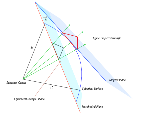
Figure 3: Projection of an equilateral triangular lattice to the tangent plane of a curved surface. Taking the perspective point to infinity (or equivalently taking the lattice spacing to zero), this projects the affine transformed triangular lattice of each tangent plane to the flat space of our current investigation.

The field of projective geometry is a vast and ancient discipline. While none of what we present in this section is original or even essential to our algebraic construction, we think it helps guide the presentation and to connect the topological structure of the action on the left side of Eq. 2 to the metric information of the simplicial complex on the right side.

2.1 Complex Projective Line

For 2d conformal field theory, the stereographic projection to the Riemann sphere [9] adds a point at complex infinity, which is a conventional model of the Complex Projective line $\mathbb{CP}(1)$. In $\mathbb{CP}(1)$ a point is defined by homogeneous coordinates $(z^{1},z^{2})\sim\lambda(z^{1},z^{2})$ in the equivalence class relative to complex scaling $\lambda$ and a line $L_{1},L_{2}$, by a linear homogeneous form, $L_{1}z^{1}+L_{2}z^{2}=0$. Thus, the automorphism of $\mathbb{CP}(1)$ is given by a 2-by-2 complex matrix with unit determinant that take lines into lines. Choosing a frame, $(z^{1},z^{2})=(z^{1}/z^{2},1)=(z,1)$, this transformation is

$$\begin{bmatrix}a&b\\ c&d\end{bmatrix}\begin{bmatrix}z\\ 1\end{bmatrix}=\begin{bmatrix}az+b\\ cz+d\end{bmatrix}\rightarrow\begin{bmatrix}(az+b)/(cz+d)\\ 1\end{bmatrix}\;.$$ (5)

The linear algebra in homogeneous coordinates is equivalent to the Möbius transform: $\;z^{\prime}=(az+b)/(cz+d)$ or the projection $GL(2,C)\rightarrow PGL(2,C)$. A key feature of the Möbius transformation on $\mathbb{R}^{2}$ is that it preserve angles and takes circles into circles with the line being a special circle of infinite radius. We note that now the point at infinity is not special, so the Riemann sphere is an elegant manifold for studying 2d conformal theories.

2.2 Real Projective Geometry and the Affine Plane

On the other hand, ${\mathbb{RP}}(2)$ is a non-orientable manifold represented by $S^{2}$ with antipodal points identified. In ${\mathbb{RP}}(d)$, a point is represented by $d+1$ real numbers up to a real scale: $X^{I}=(X^{0},X^{1},\cdots,X^{d})\equiv\lambda X^{I}$. A line is defined by the scale-invariant homogeneous relation $L_{I}X^{I}=0$, or

$$L_{1}x^{1}+L_{2}x^{2}+L_{3}x^{3}=0$$ (6)

in ${\mathbb{RP}}(2)$. Projected to a standard plane at $z=x^{3}=1$, this is a line $ax+by+c=0$ in the $x$-$y$ plane. The automorphism is a transformation with 8 real parameters,

$$\begin{bmatrix}a_{11}&a_{12}&b_{1}\\ a_{21}&a_{22}&b_{2}\\ c_{1}&c_{2}&d\end{bmatrix}\begin{bmatrix}x^{1}\\ x^{2}\\ 1\end{bmatrix}=\begin{bmatrix}a_{1j}x^{j}+b_{1}\\ a_{2j}x^{j}+b_{2}\\ {c_{j}x^{j}+d}\end{bmatrix}\rightarrow\begin{bmatrix}(a_{1j}x^{j}+b_{1})/(c_{j}x^{j}+d)\\ (a_{2j}x^{j}+b_{2})/(c_{j}x^{j}+d)\\ 1\end{bmatrix}\;.$$ (7)

More interesting is to contrast the affine 6-parameter group subgroup in ${\mathbb{RP}}(2)$ which leaves the line at infinity fixed:

$$\vec{x}^{\prime}=A\vec{x}+\vec{d}\implies\begin{bmatrix}x^{\prime}\\ y^{\prime}\\ 1\end{bmatrix}=\begin{bmatrix}a_{xx}&a_{xy}&d_{x}\\ a_{yx}&a_{yy}&d_{y}\\ 0&0&1\end{bmatrix}\begin{bmatrix}x\\ y\\ 1\end{bmatrix}$$ (8)

with the 6-parameter conformal Möbius group. Both groups extend the 4 parameters, the Poincaré group (2 translations, 1 rotation) and scaling but the 2 additional affine parameters break conformal symmetry. They do not preserve angles or map circles into circles. Instead the additional affine transformations take circles into ellipses, with the additional parameters determining the eccentricity and shear direction of the major axis. All of these observations are generalized in comparing conformal vs. affine transformation in higher dimensions.

Finally, we can contrast this with the affine subgroup of the Möbius group by fixing the complex point at infinity:

$$\begin{bmatrix}a&b\\ 0&1\end{bmatrix}\begin{bmatrix}z\\ 1\end{bmatrix}=\begin{bmatrix}az+b\\ 1\end{bmatrix}\;.$$ (9)

In real coordinates ($a=a_{r}+ia_{i}=\lambda e^{i\theta},b=b_{r},+ib_{i},z=x^{1}+ix^{2}$)

$$z^{\prime}=az+b\implies\begin{bmatrix}x^{\prime}\\ y^{\prime}\\ 1\end{bmatrix}=\begin{bmatrix}a_{r}&-a_{i}&b_{r}\\ a_{i}&a_{r}&b_{i}\\ 0&0&1\\ \end{bmatrix}\begin{bmatrix}x^{1}\\ x^{2}\\ 1\end{bmatrix}\;.$$ (10)

In 2d, this is just the 4-parameter subgroup with Euclidean Poincaré invariance plus scaling common to both groups.

While beyond our current needs, a more general approach to conformal invariance is to introduce two extra dimensions in ${\mathbb{RP}}(d+1)$, restricted to a null surface $-X^{2}_{0}+X^{2}_{d+1}+X^{2}_{s}+\cdots X^{2}_{d}=0$, invariant under the Lorentz group $O(d+1,1)$ and subsequently projected onto a light-like vector $X_{0}+X_{3}=1$ into $\mathbb{R}^{d}$. For example starting with ${\mathbb{RP}}(3)$ this induces the Möbius transformation on $z=x_{1}+ix_{2}$ identical to $\mathbb{CP}(1)$ above. Alternatively, adding two extra dimension and fixing $X^{2}_{d}=R^{2}$, the hyperbolic geometry is the manifold for Euclidean AdS^d+1 as in [10] with the $\text{CFT}^{d}$ residing at the boundary.

2.3 Simplicial Geometry and the Free CFT

The affine transformation also plays a central role in simplicial geometry and the finite element method (FEM). The FEM has a vast literature with many implementations. Here is a glimpse of the simplest and most geometrically intuitive methods based on a simplicial complex. A simplicial complex is composed of primitive $d$-simplices $\sigma_{d}(0,1,\cdots d)$ (corresponding to points, line segments, triangles, tetrahedrons, etc. for $d=0,1,2,3,\cdots$) with $d+1$ vertices and boundaries composed of $(d-1)$-simplices, glued together with the correct orientation required to define topology on the manifold. Adding edge lengths fixes a piecewise flat metric interpolation of any Riemann manifold.

All of the primitive simplices are equivalent under affine transformations. The $d(d+1)$ affine parameters match the $d+1$ position vector $x^{j}$ in $d$-dimensions. Primitive simplices are rigid objects. Exactly half of the $d(d+1)$ parameters define the simplex shape determined completely by their $d(d+1)/2$ edge lengths. The other half are the Poincaré rotations and translations to locate and orient the simplex. This decomposition is easily understood in terms of the SVD form, $x=Ax+b\equiv U\Sigma V+b$, where $U,V$ are rotations and the $d$ diagonal singular values (or shearing parameters) transform circles into ellipsoids.

The flat interpolation of the interior of each simplex is parameterized by $d$ affine invariant barycentric coordinates $\xi_{j}$

$$X(\xi_{i})=\xi_{0}x^{0}+\xi_{1}x^{1}+\cdots+\xi_{d}x^{d}\quad,\quad\xi_{0}+\xi_{1}+\cdots+\xi_{d}=1\;.$$ (11)

The discrete algebraic properties of a simplicial complex and its Voronoi dual are remarkable, allowing the simplicial analogue of exterior derivative, Hodge star, Stokes’ theorem etc. There is a sequence of simplicial objects $\sigma_{0},\sigma_{1},\cdots,\sigma_{d}$ (points, lines, triangles, etc.) and their Voronoi duals $\sigma^{*}_{d},\cdots\sigma^{*}_{1},\sigma^{*}_{0}$, respectively, which are constructed recursively from circumcenters. The circumcenters are found by the intersection of perpendicular lines which gives the simplicial analogue of the $\epsilon^{i_{1},i_{2},\cdots,i_{d}}$ symbol central to both projective geometry and exterior calculus. For more details the reader is referred to Ref. [4] and the classical papers for random lattices in flat space by Christ, Friedberg and T.D. Lee [11, 12, 13].

Applied to the continuum free scalar action,

$$S=\textstyle{\frac{1}{2}}\int_{\cal M}d^{d}x\sqrt{g}\left[\;g^{\mu\nu}\partial_{\mu}\phi(x)\partial_{\nu}\phi(x)\\ +\left(m^{2}+\frac{(d-2)\text{Ric}}{4(d-1)}\;\phi^{2}(x)\right)\right]\;,$$

the simplest FEM approximation adds a piecewise linear approximation (11) to the manifold and a piecewise linear basis for the scalar fields in the interior of each simplex (e.g. triangle), $\phi(x)=\sum_{i}\xi_{i}\phi_{i}$. Performing the integral in this basis gives

$$S^{\text{(kin.)}}_{\triangle}=\frac{\ell^{2}_{23}+\ell^{2}_{31}-\ell^{2}_{12}}{8A_{\triangle}}(\phi_{1}-\phi_{2})^{2}+(23)+(31)=\frac{1}{2}\frac{A_{12}}{\ell^{2}_{12}}(\phi_{1}-\phi_{2})^{2}+(23)+(31)$$ (12)

for the kinetic term for the triangle $\triangle(1,2,3)$ with edge lengths $\ell_{12},\ell_{23},\ell_{31}$ and area $A_{\triangle}$. The intuitively appealing form on the right side of Eq. 12 expresses the contribution to an edge from a single triangle as the area, $A_{12}=(\ell_{12}/2)\sqrt{R^{2}+(\ell^{2}_{12}/2)}$ divided by the edge length squared, as illustrated on the left of Fig. 4. The organization of this geometry in any dimension on any manifold is the first job of the discrete exterior calculus (DEC). In 2d, summing over any closed surface, the scalar action is

$$S_{\text{FEM}}=\frac{1}{2}\sum_{\langle ij\rangle}\frac{\ell^{*}_{ij}}{2\ell_{ij}}\;(\phi_{i}-\phi_{j})^{2}$$ (13)

where $\ell^{*}_{ij}$ is the distance between circumcenters of the adjacent triangles sharing the edge $\langle ij\rangle$. In the language of DEC, the equation of motion is the discrete simplicial Beltrami-Laplace operator

$$*d*d\phi_{i}=*\frac{1}{|\sigma^{*}_{0}(i)|}\int_{\sigma^{*}_{0}}d[*(\phi_{i}-\phi_{j})/\ell_{ij}]=\frac{1}{\sqrt{g_{i}}}\sum_{j\in\langle i,j\rangle}\ell^{*}_{ij}\frac{\phi_{i}-\phi_{j}}{\ell_{ij}}\;.$$ (14)

with a positive semi-definite spectrum and one null vector given by $\phi_{i}=\mbox{const}$. The discrete exterior derivative of a scalar is $d\phi_{i}=(\phi_{j}-\phi_{i})/\ell_{ij}$ on the $\langle i,j\rangle$ link and the integral is a simplicial Stokes’ theorem evaluated as the flux out of the dual Voronoi polyhedron as illustrated in Fig. 4 for 2d.

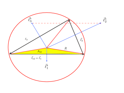
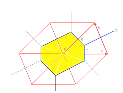
Figure 4: On the left is a general triangle defined by three vectors satisfying $\vec{\ell}_{1}+\vec{\ell}_{2}+\vec{\ell}_{3}=0$ and circumscribed by the circle in red. In yellow is the triangular area $A_{12}$ assigned to the free scalar FEM action. On the right is the discrete simplicial Beltrami-Laplace operator evaluated by flux for the Voronoi hexagonal boundary in black for our affine lattice.

In Fig. 4 we have chosen to illustrate the special case of our uniform triangles which imposes the identity, $\vec{\ell}_{i}=\epsilon^{ijk}(\vec{\ell}^{*}_{j}-\vec{\ell}^{*}_{k})/2$, and the three FEM couplings in Eq. 2:

$$2K_{1}=\ell^{*}_{1}/\ell_{1}\quad,\quad 2K_{2}=\ell^{*}_{2}/\ell_{2}\quad,\quad 2K_{3}=\ell^{*}_{3}/\ell_{3}\;.$$ (15)

These projective methods have a huge application domain, which includes a natural connection to simplicial geometry [14] and the discrete exterior calculus under the rubric of conformal geometric algebra [15].

3 Star-Triangle Identity

The star-triangle identity is a pure graph-theoretical result, mapping between Ising spins on triangular and hexagonal graphs [16, 17]. There is no reference to distances or any metric. To set conventions, consider the Ising model defined on a general graph $G(N,E)$ with $N$ sites and $E$ undirected edges (or links) $\langle n,m\rangle\in G$ and partition function,

$$Z^{G}_{N}[K]=\sum_{s_{n}=\pm 1}\exp\bigg{[}\sum_{\langle n,m\rangle}K_{nm}s_{n}s_{m}\bigg{]}\equiv\operatorname{Tr}_{s}\bigg{[}e^{\textstyle K_{nm}s_{n}s_{m}}\bigg{]}$$ (16)

where couplings with $K_{nm}=0$ imply the absence of links in graph.

Specializing to a triangular graph and its dual hexagonal graph illustrated in Fig. 1, each with three distinct couplings $K_{1},K_{2},K_{3}$ and $L_{1},L_{2},L_{3}$, respectively, gives

$$Z^{\triangle}_{N}(K)=\operatorname{Tr}_{s}\bigg{[}e^{\textstyle K_{1}s_{n}s_{n+\hat{1}}+K_{2}s_{n}s_{n+\hat{2}}+K_{3}s_{n}s_{n+\hat{3}}}\bigg{]}$$ (17)

and

$$Z^{\hexagon}_{N}(L)=\operatorname{Tr}_{s}\bigg{[}e^{\textstyle\sum_{n/2}L_{1}s_{n}s_{n+\hat{1}}+L_{2}s_{n}s_{n+\hat{2}}+L_{3}s_{n}s_{n+\hat{3}}}\bigg{]}\;.$$ (18)

The index $n+\hat{i}$ for $i=1,2,3$ enumerates the distinct non-zero links $\langle n,n+\hat{i}\rangle$. For high temperature power series expansion we introduce the parameters $v_{i}=\tanh(K_{i})$ and $t_{i}=\tanh(L_{i})$. The star-triangle identity gives an exact map between the two partition functions.

Starting with the hexagonal graph, we note that it is bipartite (see Fig. 5),

Figure 5: On the left the bipartite structure of the hexagonal graph with its coupling parameters $L_{1},L_{2},L_{3}$ and on right the star-triangle map to the triangular graph with coupling constants $K_{1},K_{2},K_{3}$.

coupling black and white sites. Consequently we may decimate the hexagonal graph by summing over each white spin and projecting it onto the triangular model. For example, suppose a specific spin $s_{0}$ on a white vertex is connected to the neighboring black spin $s_{1},s_{2},s_{3}$ by edges with couplings $L_{1},L_{2},L_{3}$ as illustrated in Fig. 5 on the right. The result is the local star-triangle identity

$$\sum_{s_{0}=\pm 1}e^{\textstyle L_{1}s_{0}s_{1}+L_{2}s_{0}s_{2}+L_{3}s_{0}s_{3}}={\cal D}e^{\textstyle K_{1}s_{2}s_{3}+K_{2}s_{3}s_{1}+K_{3}s_{1}s_{2}}$$ (19)

with ${\cal D}^{2}=2h\sinh 2L_{1}\sinh 2L_{2}\sinh 2L_{3}$. Obviously both the RHS and LHS side of Eq. 19 can be expanded into four terms: $c_{0}+c_{1}s_{2}s_{3}+c_{2}s_{3}s_{1}+c_{3}s_{1}s_{2}$. Choosing four independent configurations $(s_{1},s_{2},s_{3})=(1,1,1),(-1,1,1),(1,-1,1),(1,1,-1)$ determines a 4 parameter map: $(L_{1},L_{2},L_{3},{\cal D})$ $\leftrightarrow$ $(K_{1}K_{2},K_{3},h)$. The algebra is intricate and is probably best understood as special case of the soluble models and the Yang-Baxter relation [16], nonetheless the result is given by

$$h(K_{1},K_{2},K_{3})=\frac{(1-v_{1}^{2})(1-v_{2}^{2})(1-v_{3}^{2})}{4\sqrt{(1+v_{1}v_{2}v_{3})(v_{1}+v_{2}v_{3})(v_{2}+v_{3}v_{1})(v_{3}+v_{1}v_{2})}}$$ (20)

with $v_{i}=\tanh(K_{i})$ and

$$h\sinh(2K_{1})\sinh(2L_{1})=h\sinh(2K_{2})\sinh(2L_{2})=h\sinh(2K_{3})\sinh(2L_{3})=1\;.$$ (21)

The consequence is an exact equivalence of the hexagonal and triangular partition functions for all values of the couplings,

$$Z^{\hexagon}_{2N}(L_{i})={\cal D}^{N}Z^{\triangle}_{N}(K_{i})=(2h\sinh(2L_{1})\sinh(2L_{2})\sinh(2L_{3}))^{N/2}Z^{\triangle}_{N}(K_{i})\;.$$ (22)

Note that this is a graph-theoretic result giving a one-to-one mapping: $L_{i}\leftrightarrow K_{i}$. Although there is no need for a reference to distances, if the vertices can be placed at regular intervals in $\mathbb{R}^{2}$, in the spirit of Wilsonian blocking both partition functions will share a second order critical point. If such a point exists, the theories will have identical correlation functions in the infrared.

The next step is to find the critical surface, assuming there is a single transition, which is well known in the limit of the triangular ($K_{1}=K_{2}=K_{3}$) and square ($K_{1}=K_{2},K_{3}=0$) lattice Ising models. The procedure is a generalization of the Kramers-Wannier duality [18], comparing the weak coupling (high temperature) expansion on the triangular Ising graph with the strong coupling (low temperature) expansion on the hexagonal graph. At high temperature, expanding in $v_{i}=\tanh(K_{i})$ on the triangular graph, we have

$$Z^{\triangle}_{N}(K)=(\cosh K_{1}\cosh K_{2}\cosh K_{3})^{N}\operatorname{Tr}_{s}\bigg{[}\prod_{\langle n,i\rangle}\left(1+v_{i}s_{n}s_{n+\hat{i}}\right)\bigg{]}\;.$$ (23)

The notation $\langle n,i\rangle$ is used to specify the undirected link $\langle n,m\rangle=\langle n,m=n+\hat{i}\rangle$. Summing over the spins, we must pair spins on each site, giving all paths ${\cal P}$ with a product of links weighted by $v_{i}$.

Now compare with the hexagonal graph, expanding at low temperature in powers of $q_{i}=e^{-2L_{i}}$ ,

$$Z^{\hexagon}_{2N}(L_{i})=e^{N(L_{1}+L_{2}+L_{3})}\operatorname{Tr}_{s}\bigg{[}\prod_{n,i}\left(q_{i}+(1-q_{i})\delta_{s_{n},s_{n+\hat{i}}}\right)\bigg{]}\;,$$ (24)

where we have used the identity: $e^{L_{i}s_{n}s_{n+\hat{i}}}=e^{L_{i}}[q_{i}+(1-q_{i})\delta_{s_{n},s_{n+\hat{i}}}]$. The sum over spins enumerates the number of broken (anti-parallel) bonds entering and exiting each hexagon on the dual triangular lattice. Since the $N$-site triangular graph is dual to the $2N$-site hexagonal graph, the loop expansions are identical at $e^{-2L_{i}}\equiv\tanh(K_{i})$ proving,

$$Z^{\hexagon}_{2N}(L_{i})=(2\sinh 2L_{1}\sinh 2L_{2}\sinh 2L_{3})^{N/2}Z^{\triangle}_{N}(K_{i})\;.$$ (25)

Convergence is subtle but we assume a proper limit to the critical surface. Combining the star-triangle identity (22) and the duality condition (25) proves that if there is a single common phase boundary for both the hexagonal and triangular partition functions, the critical surface satisfies $h(K_{1},K_{2},K_{3})=1$ and the duality map $\sinh 2K_{i}\sinh 2L_{i}=1$. Introducing the pair of high/low expansion coefficients

$$v_{i}=\tanh(K_{i})\;,\;p_{i}=e^{-2K_{i}}\quad\mbox{and }\quad t_{i}=\tanh(L_{i})\;,\;q_{i}=e^{-2L_{i}}$$ (26)

for the triangular and hexagonal models respectively this is equivalent to the duality condition $p_{i}=t_{i}$ or $q_{i}=v_{i}$.

Setting $h=1$ in Eq. 20 results in a 12th order polynomial [16], in $v_{i}=\tanh(K_{i})$ but we find that this is can be reduced to an elegant form  

$$p_{1}p_{2}+p_{2}p_{3}+p_{3}p_{1}=1\quad\mbox{with}\quad p_{i}=\exp(-2K_{i})$$ (27)

for the physically relevant roots. Equivalently, for the hexagonal lattice the surface is

$$t_{1}t_{2}+t_{2}t_{3}+t_{3}t_{1}=1\quad\mbox{with}\quad t_{i}=\tanh(L_{i})\;.$$ (28)

This has several interesting properties. These probability weights ($0<p_{i}\leq 1$) enter the Swendsen-Wang cluster algorithm to cut bonds between aligned spins [19]. Likewise $q_{i}=\exp(-2L_{i})$ are dual Swendsen-Wang probabilities on the hexagonal lattice. They obey a symmetric Möbius map $p_{i}=(1-q_{i})/(1+q_{i})$ and $q_{i}=(1-p_{i})/(1+p_{i})$.

The question we raise in Sec. 4 is whether the dynamics induces a metric for correlation functions. More specifically,

• For the critical theory, is there a lattice metric (e.g. a set of edge lengths) that restores rotational symmetry on $\mathbb{R}^{2}$ on the critical surface?

• Is this map on the finite torus consistent with modular invariance for the continuum $c=1/2$ minimal CFT?

Both of these we answer in the affirmative and support by numerical evidence.

4 Wilson-Majorana Fermionic Solution

In order to find the induced metric at the critical point (27), we use a special property of the 2d Ising model. The partition function can be represented on the graph as a free Wilson-Majorana fermion [20], which is a free CFT at the critical point and fixes the emergent geometry by FEM methods [3]. Our approach follows Wolff’s elegant paper [21] on the fermionic representation of the uniform hexagonal lattice generalized to the 3 parameter coupling space: $L_{1},L_{2},L_{3}$. Wolff notes that the loop expansion on the hexagonal lattice is simpler than that of the square or triangular lattice because there are no self-intersections due to the trivalent form shown in Fig. 6.

Figure 6: Hexagonal lattice used in our derivation showing the bipartite and trivalent structure.

Indeed this argument can be extended to any trivalent dual of a triangular simplicial graph, but for simplicity we restrict the analysis to our three parameter hexagonal graph.

The high temperature expansion in $t_{i}=\tanh L_{i}$ is

$$Z^{\hexagon}_{N}(L_{i})=\operatorname{Tr}_{s}\bigg{[}e^{\textstyle\sum_{\langle n,i\rangle}L_{i}\,s_{n}s_{n+\hat{i}}}\bigg{]}=(\cosh L_{1}\cosh L_{2}\cosh L_{2})^{N/2}\;\operatorname{Tr}_{s}\bigg{[}\prod_{\langle n,i\rangle}(1+t_{i}s_{n}s_{n+\hat{i}})\bigg{]}\;.$$ (29)

Again the notation $\langle n,i\rangle$ implies a product over each undirected link, or equivalently the restriction of $n$ to blue sites only. Summing over the spins leads to a loop expansion of all non-self intersecting closed paths ${\cal P}$ of length $\Lambda=n_{1}+n_{2}+n_{3}$ with power $t_{1}^{n_{1}}t_{2}^{n_{2}}t_{3}^{n_{3}}$.

We now introduce a hexagonal lattice action for Wilson-Majorana Fermions,

$$S[\psi]=\dfrac{1}{2}\sum_{n}\bar{\psi}_{n}\psi_{n}-\sum_{n,i}\kappa_{i}\bar{\psi}_{n}P(\hat{e}_{i})\psi_{n+\hat{i}}$$ (30)

and demonstrate that its partition function

$$Z^{\psi}_{N}=\prod_{n}\iint d\psi^{1}_{n}d\psi^{2}_{n}\;e^{\textstyle-S[\bar{\psi},\psi]}=\prod_{n}\int d^{2}\psi_{n}e^{\textstyle-\frac{1}{2}\sum_{n}\bar{\psi}_{n}\psi_{n}}\prod_{n,i}\left[1+\kappa_{i}\bar{\psi}_{n}P(\hat{e}_{i})\psi_{n+\hat{i}}\right]$$ (31)

expanded in $\kappa_{i}$ matches the Ising loop expansion (29) term by term. For the sums and products of nearest-neighbor spinors above, it is understood that each directed link is included only once. The Wilson link matrices are

$$P(\hat{e}_{i})=\frac{1}{2}(1+\hat{e}_{i}\cdot\vec{\sigma})\quad,\quad\vec{\sigma}=(\sigma_{1},\sigma_{2})\;.$$ (32)

The introduction of unit vectors $\hat{e}_{i}$ is intentional. In general, Fermionic spinors on a simplicial complex (e.g a triangulated lattice) require tangent vectors $\hat{e}_{i}$ for the lattice vierbein $E_{i}=\hat{e}_{i}\cdot\vec{\sigma}$. Because we anticipate a critical theory in flat space, the tangent vectors on all planes can be given in global coordinates in a gauge with zero spin connection.

In order for the Grassmann integral in Eq. 31 to match the non-self intersecting loop expansion, there must be only two fermionic variables per site. This is accomplished by replacing 4 Grassmann Dirac variables $\bar{\psi},\psi$ by 2 Wilson-Majorana fermions [21] that obey the charge conjugation constraint, $\bar{\psi}=\psi^{T}{\cal C}$:

$${\cal C}=-i\sigma_{2}=\begin{bmatrix}0&1\\ -1&0\end{bmatrix}\quad,\quad\bar{\psi}^{1}=-\psi^{2}\quad\mbox{and}\quad\bar{\psi}^{2}=\psi^{1}$$ (33)

or $\bar{\psi}^{j}=\psi^{i}\epsilon_{ij}$ with the epsilon operator, ${\cal C}_{ij}=\epsilon_{ij}$. The mass term is

$$e^{\textstyle-\frac{1}{2}\sum_{n}\bar{\psi}_{n}\psi_{n}}=\prod_{n}\left[1-\frac{1}{2}\psi^{i}_{n}\epsilon_{ij}\psi^{j}_{n}\right]=\prod_{n}\left[1-\frac{1}{2}(\psi^{1}_{n}\psi^{2}_{n}-\psi^{2}_{n}\psi^{1}_{n})\right]$$ (34)

and the Grassmann measure at each site is defined as $d^{2}\psi_{n}=d\psi^{1}_{n}d\psi^{2}_{n}$.

To generate the loop expansion, we compute the product of Wilson matrices. In flat 2d space with no-self intersections, the winding number is $\pm 1$ resulting in a spinor phase $\exp[i\theta/2]=-1$ with $\theta=\pm 2\pi$. The minus sign is cancelled by the anti-commutation of the Grassmann measure over the closed path . To make this concrete we will carry this out explicitly. In global coordinates, defining $\hat{e}_{i}=(\cos\theta_{i},\sin\theta_{i})$, the Wilson factor is a (dyadic) projection matrix:

$$P(\hat{e}_{i})=\frac{1}{2}(1+\hat{e}_{i}\sigma)=\frac{1}{2}\begin{bmatrix}1&e^{-i\theta_{i}}\\ e^{i\theta_{i}}&1\end{bmatrix}=\frac{1}{2}\begin{bmatrix}1\\ e^{i\theta_{i}}\end{bmatrix}\begin{bmatrix}1&e^{-i\theta_{i}}\end{bmatrix}\;.$$ (35)

This gives a spinor rotation phase at each corner,

$$R_{z}(\theta_{21})=\frac{1}{2}\begin{bmatrix}1&e^{-i\theta_{1}}\end{bmatrix}\begin{bmatrix}1\\ e^{i\theta_{2}}\end{bmatrix}=\cos(\theta_{12}/2)e^{i(\theta_{2}-\theta_{1})/2}$$ (36)

by $(\theta_{2}-\theta_{1})/2$ at each vertex giving rise to a minus sign (or by $e^{i\pi}=-1$) for any closed loop. Incidentally in 1983 the Ising Wilson-Majorana links representation was generalized by Brower, Giles and Maturana [22] to Wilson Fermions in 4d lattice QCD. On the 4d hypercubic lattice, the Wilson link projectors, $P_{\mu}=(1+\gamma_{\mu})/2$, mapped to spinor rotations $R_{\mu\nu}=\exp[i\pi\sigma_{\mu\nu}/4]$ by $\pi/4$ at each corner in the $\mu$-$\nu$ plane, giving the appropriate minus sign to Fermion loops.

Finally, matching the amplitudes of the loop expansion requires corners with weights

$$\sqrt{t_{i}t_{j}}=\sqrt{\kappa_{i}\kappa_{j}}\cos(\theta_{ij}/2)\quad,\quad\theta_{ij}=\theta_{j}-\theta_{i}$$ (37)

or

$$t_{1}=\frac{\kappa_{1}\cos(\theta_{12}/2)\cos(\theta_{13}/2)}{\cos(\theta_{23}/2)}=\tanh(L_{1})\;.$$ (38)

It might be interesting to pursue generalizations of this fermionic loop expansion for general 2d surfaces. In 2d any triangulated simplicial complex has a trivalent dual graph leading to a dual non-self-intersecting loop expansion, but curvature requires the inclusion of a spin connection following the general method in Ref. [3] with manifest gauge invariance with rotation of the tangent vector at each site. Similar methods have been used in the random triangulation solution to 2d string theory [23].

4.1 Matching Geometry to Critical CFT on $\mathbb{R}^{2}$

To introduce the full metric information for each hexagonal edge with coupling constant $L_{i}$, we assign a 2d vector $\vec{a}_{i}=a_{i}\hat{e}_{i}$ leaving solid black sites as shown on the left in Fig. 7. We then use the star triangle map on the right side of Fig. 7 to assign edges to the triangular model,

$$\vec{\ell}_{1}=\vec{a}_{2}-\vec{a}_{3}\quad\mbox{ and cyclic}$$ (39)

or equivalently $\vec{\ell}_{k}=\epsilon_{ijk}(\vec{a}_{i}-\vec{a}_{j})/2$ on the triangular lattice. Note that this implies correctly the triangle condition $\vec{\ell}_{1}+\vec{\ell}_{2}+\vec{\ell}_{2}=0$.

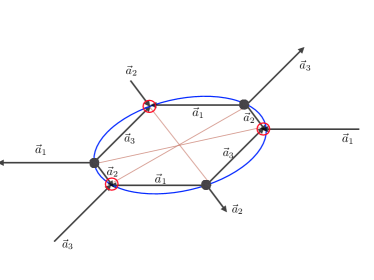
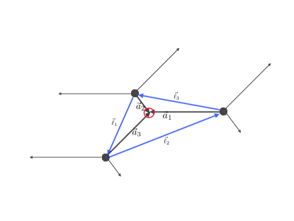
Figure 7: On the left, the edge lengths of parallel links on the hexagonal lattice define a simplicial matrix which on the right is applied to the triangular lattice using the star-triangle relation: $\vec{\ell}_{k}=\epsilon^{ijk}(\vec{a}_{i}-\vec{a}_{j})/2$.

This is not a one-to-one map. The geometry for our hexagonal lattice with opposite parallel edges requires 6 parameters for the three vectors $\vec{a}_{i}$, while the triangular lattice requires only 4 parameters. Our hexagons are special in that they lie on the boundary of an ellipse which is therefore an example of Pascal’s theorem [24], and requires that the intersections of three pairs of lines for the opposite sides lie on single line. However in our case with parallel opposite sides the intersections are all on a line at infinity in projective space.

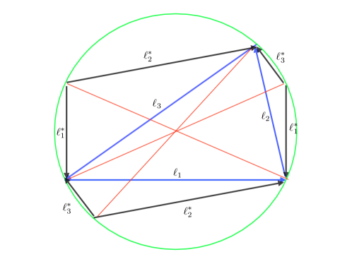
Figure 8: Coincident triangle (blue) and hexagon (black) circumscribed by a circle of radius $R$ in green. The dual Voronoi vectors $\vec{\ell}^{*}_{i}$ are orthogonal to the triangles vectors $\vec{\ell}_{i}$ with magnitude satisfying $4R^{2}=\ell^{*2}_{i}+\ell^{2}_{i}$.

The two extra degrees of freedom correspond to eccentricity and the direction of the major axis which exist in the affine transformation of circles to ellipses. The affine transformation of the ellipse to a circle is precisely the metric required to restore full conformal symmetry on the critical surface and the ambiguity of the inverse map is fixed by requiring the hexagons to be cyclic polygons, i.e. corresponding to the Voronoi dual of the triangular lattice. This is illustrated in Fig. 8 showing how the new hexagons and the triangles can both be circumscribed by identical circles.

We now turn to the algebraic proof of this statement, aware of the fact that there are surely more elegant methods which directly use projective geometry beyond our current presentation.

Our problem is to find metric values for $\vec{a}_{i}$ that restore rotational symmetry on the critical surface. Remarkably, this constrains the hexagonal vectors to be at the circumcenter dual to the triangular complex, $\vec{a}_{i}=\vec{\ell}^{*}_{i}$ where $*$ is the Hodge star of the discrete exterior calculus (DEC) for the finite element method (FEM) applied to the free Laplacian in Eq. 14.

In anticipation of taking the continuum limit, we introduce position vectors $x^{\mu}$ with neighboring sites at $y^{\mu}=x^{\mu}+a^{\mu}_{i}$. Changing notation to $\kappa_{i}\rightarrow\kappa_{xy}$ and $\hat{e}_{i}\rightarrow\hat{e}_{xy}$ on each link $\langle x,y\rangle$, the fermion action is written

$$S=\dfrac{1}{2}\left[\sum_{x}\bar{\psi}_{x}\psi_{x}-\sum_{\langle x,y\rangle}\kappa_{xy}\bar{\psi}_{x}\psi_{y}-\sum_{\langle x,y\rangle}\kappa_{xy}\bar{\psi}_{x}\hat{e}_{xy}\cdot\vec{\sigma}\psi_{y}\right]\;.$$ (40)

The second term,

$$\sum_{\langle x,y\rangle}\kappa_{xy}\bar{\psi}_{x}\psi_{y}=\sum_{\langle x,y\rangle}\kappa_{xy}\bar{\psi}_{x}\psi_{x}-\frac{1}{2}\sum_{\langle x,y\rangle}(\bar{\psi}_{x}-\bar{\psi}_{y})(\psi_{x}-\psi_{y})\simeq\frac{1}{2}\sum_{i}\kappa_{i}\sum_{x}\bar{\psi}_{x}\psi_{x}$$ (41)

is a mass correction plus a second derivative term which vanishes as the square of the lattice spacing in the continuum. Similarly we may expand the third term in (40) using

$$\psi_{y}=\psi_{x}+a_{xy}\hat{e}_{xy}\cdot\vec{\nabla}\psi_{i}+\mathcal{O}(a^{2}_{i})\;.$$ (42)

Defining $m_{0}=1-\sum_{i}\kappa_{i}/2$ and noting that $\bar{\psi}_{x}\vec{\sigma}\psi_{x}=0$ we have

$$S=\dfrac{1}{2}\left[\sum_{\langle xy\rangle}\bar{\psi}_{x}(\hat{e}_{xy}\cdot\vec{\sigma})(\kappa_{xy}a_{xy}\hat{e}_{xy}\cdot\vec{\nabla})\psi_{x}+m_{0}\sum_{x}\bar{\psi}_{x}\psi_{x}\right]+\mathcal{O}(a_{i}^{2})\;.$$ (43)

Near a second order phase we fix the physical mass $m$ by scaling $m_{0}=\sqrt{g_{x}}m$, where on our regular lattice $\sqrt{g_{x}}=2A_{\triangle}$, the area of the triangle dual to each lattice site on the hexagonal lattice.

Finally, to restore spherical symmetry we must adjust the metric to satisfy

$$\sum_{i}aE_{i}\partial_{i}=\sum_{i}(\kappa_{i}\hat{e}_{i}\cdot\vec{\sigma})(\vec{a}_{i}\cdot\vec{\nabla})\sim\vec{\sigma}\cdot\vec{\nabla}\;.$$ (44)

The solution has a remarkably elegant geometric form by scaling the vectors $a\partial_{i}=\vec{a}_{i}\cdot\nabla=\ell^{*}_{i}\hat{e}_{i}\cdot\nabla$ aligned along the circumcenter dual edges to the triangular lattice with edges lengths, $\ell_{1},\ell_{2},\ell_{3}$ as shown in Fig. 8. Now $\ell^{*}_{i}$ is the Hodge star of the edge simplex with length $\ell_{i}$ and vierbein $\vec{E}_{i}=\kappa_{i}\hat{e}\cdot\vec{\sigma}=\ell_{i}\hat{e}_{i}\cdot\vec{\sigma}$ scaled to the triangular edges. As illustrated in Fig. 8, corresponding hexagonal and triangular vectors are orthogonal. Therefore the vierbein $\vec{E}_{i}=-i\sigma_{2}\vec{\ell}_{i}\cdot\vec{\sigma}$ is rotated by 90 degrees relative to $\vec{\ell}_{i}$, in agreement with charge conjugation of the Wilson-Majorana spinor frame. The result is that the Hodge duality fixes the vectors to the circumcenter of the dual triangular simplex.

$$\ell^{*\mu}_{1}=\epsilon^{\mu\nu}\ell^{\nu}_{1}(\ell^{2}_{2}+\ell^{2}_{3}-\ell^{2}_{1})/(4A_{\triangle})\quad,\quad\mbox{1, 2, 3 cyclic}$$ (45)

This is a 2d example of the general property of Hodge duality in the FEM discrete exterior calculus for any simplicial complex and its circumcenter dual. We define a global lattice scale $a$ by the dual area of sites in the triangular lattice: $a^{2}=\sqrt{g_{x}}=2A_{\triangle}$.

A geometric calculation, easily visualized in the right side of Fig. 4 gives

$$\sum_{i}\ell^{\mu}_{i}\ell^{*\nu}_{i}=2A_{\triangle}\epsilon^{\mu\nu}$$ (46)

where $2A_{\triangle}=\vec{\ell}^{*}_{1}\wedge\vec{\ell}^{*}_{2}+\vec{\ell}^{*}_{2}\wedge\vec{\ell}^{*}_{3}+\vec{\ell}^{*}_{3}\wedge\vec{\ell}^{*}_{1}$. Note the dual area $A_{\hexagon}=2A_{\triangle}=\ell^{*}_{1}\ell_{1}+\ell^{*}_{2}\ell_{2}+\ell^{*}_{3}\ell_{3}$.

Introducing the canonical fermion mass $m=m_{0}/\sqrt{2A_{\triangle}}$ and rescaling $\bar{\psi}_{x}\psi_{x}\rightarrow\sqrt{2A_{\triangle}}\bar{\psi}_{x}\psi_{x}$, the sum becomes an integral with continuum action

$$S\simeq\frac{1}{2}\int d^{2}x\bar{\psi}_{x}(\vec{\sigma}\cdot\vec{\nabla}+m)\psi_{x}$$ (47)

and the critical surface at $m=0$ is given by the constraint

$$\kappa_{i}=\frac{2\ell_{i}}{\ell_{1}+\ell_{2}+\ell_{3}}=\frac{\ell_{i}}{s}\qquad,\quad\kappa_{1}+\kappa_{2}+\kappa_{3}=2$$ (48)

defining the semi-perimeter $s=(\ell_{1}+\ell_{2}+\ell_{3})/2$. The kinetic term fixes the geometry with

$$\sinh(2K_{i})=1/\sinh(2L_{i})=\frac{\ell^{*}_{i}}{\ell_{i}}\;.$$ (49)

This general solution simplifies for the regular triangular lattice with $\ell^{*}_{i}/\ell_{i}=1/\sqrt{3}$ giving the critical point $K_{i}=\ln(3)/4$. More interesting is the limit to rectangular lattice with lattices spacing, $a_{x}=\ell_{1}=\ell^{*}_{2}t$, $a_{t}=\ell_{2}=\ell^{*}_{1}$, respectively. This is the $\ell^{*}_{3}\rightarrow 0$ limit with action

$$S=\frac{1}{2}\sum_{x,t}\left[K_{t}s_{t,x}s_{t+1,x}+K_{x}s_{t,x}s_{t,x+1}\right]\;.$$ (50)

From Eq. 27, the critical surface is $\sinh(K_{t}+K_{x})=\cosh(K_{t}-K_{x})$.

From Fig. 8, we can visualize the limit $\ell^{*}_{3}\rightarrow 0$ which forces the diagonal on the triangle to vanish ($K_{3}=0$) and pairs of hexagonal spins to be free ($L_{3}\rightarrow\infty$) so the dual is triangular rectangle is a hexagonal rectangle, exchanging: $a_{t}\leftrightarrow a_{x}$. As mentioned in Sec. 5.3, these asymmetric lattices are very useful for radial quantization and finite temperature simulation.

4.2 Algebraic Derivation

The algebraic manipulations to prove Eq. 49 use standard properties of triangles with sides $\ell_{1},\ell_{2},\ell_{3}$. Heron’s formula and the circumradius

$$A_{\triangle}=\sqrt{s(s-\ell_{1})(s-\ell_{2})(s-\ell_{3})}\quad,\quad R=\frac{\ell_{1}\ell_{2}\ell_{3}}{4A_{\triangle}}$$ (51)

respectively with $s=(\ell_{1}+\ell_{2}+\ell_{3})/2$ as well as the half angle formula for $\theta_{23}$ opposite the side from $\ell_{1}$ triangle

$$\cot(\theta_{23}/2)=\sqrt{\frac{s(s-\ell_{1})}{(s-\ell_{2})(s-\ell_{3})}}\;,$$ (52)

plus permutations. Putting this together we have

$$t_{1}=\frac{\ell_{1}}{s}\frac{\cos(\theta_{12}/2)\cos(\theta_{13}/2)}{\cos(\theta_{23}/2)}=\frac{\ell_{1}}{s}\sqrt{\frac{s(s-\ell_{3})s(s-\ell_{2})}{s(s-\ell_{1})^{3}}}=\frac{4A_{\triangle}}{\ell^{2}_{2}+\ell^{2}_{3}-\ell^{2}_{1}+2\ell_{2}\ell_{3}}=\frac{\ell_{1}}{\ell^{*}_{1}+2R}\;.$$ (53)

As a consistency check, using our identity in Eq. 49 we have

$$t_{1}=\tanh(L_{1})=\frac{\sinh(2L_{1})}{1+\cosh(2L_{1})}=\frac{\ell_{1}/\ell^{*}_{1}}{1+\sqrt{1+(\ell_{1}/\ell^{*}_{1})^{2}}}=\frac{\ell_{1}}{\ell^{*}_{1}+2R}\;.$$ (54)

Finally, one can show that the zero mass conformal invariant free fermion, $\sum_{i}\kappa_{i}=\sum_{i}\ell_{i}/s=2$, is equivalent to the star-triangle critical surface

$$t_{1}t_{2}+t_{2}t_{3}+t_{3}t_{1}=\frac{\ell_{1}\ell_{2}}{(\ell^{*}_{1}+2R)(\ell^{*}_{2}+2R)}+\frac{\ell_{2}\ell_{3}}{(\ell^{*}_{2}+2R)(\ell^{*}_{3}+2R)}+\frac{\ell_{3}\ell_{1}}{(\ell^{*}_{3}+2R)(\ell^{*}_{1}+2R)}=1$$ (55)

in Eq. 27 with $t_{i}=p_{i}$. This is an interesting identity relating a triangular lattice and its Voronoi dual. Since, as illustrated in Fig. 8, the triangular lengths $\ell_{i}$ and their circumcenter dual lengths $\ell^{*}_{i}$ are fixed entirely by parallel lines and right angles, it must be a consequence of projective geometry theorems in ${\mathbb{RP}}(2)$ which would be interesting to identify and generalize to higher dimensions.

5 Monte Carlo Simulations

In this section we use our formalism to perform Monte Carlo simulations of three interesting examples of the critical Ising model: the finite modular torus $\mathbb{T}^{2}$, the infinite Euclidean plane $\mathbb{R}^{2}$ (via finite-size scaling), and the cylinder $\mathbb{R}\times S^{1}$ of radial quantization [25]. Of course, any simulation must start with a finite lattice, so the traditional test of a CFT on $\mathbb{R}^{2}$ uses an $L\times L$ periodic lattice (i.e. a torus) in the limit where the longest correlation length $\xi$ satisfies $a\ll a\xi\ll aL$ in units of the lattice spacing $a$. Technically, this should be an extrapolation for the double limit – first the infinite volume limit $L\rightarrow\infty$ followed by the approach to the critical surface $\xi\rightarrow\infty$ for a CFT or massive theory. However, our affine lattice is also ideal for comparison with the exact finite volume effects of the modular invariance of the torus going to the pseudo-critical surface as we take $L\rightarrow\infty$. Lastly, we consider briefly the advantage of the approach to the infinite cylinder $\mathbb{R}\times S^{1}$ of radial quantization, or in the limit $L_{t}\gg L_{x}$ for finite temperature. All of these have interesting consequences beyond this first test and will be pursued further with an eye to higher dimensions.

For all of our simulations, we perform 2000 thermalization sweeps followed by 50,000 measurement sweeps, with 20 sweeps between measurements. Each sweep consists of 5 Metropolis updates and 3 Wolff cluster updates [26, 27]. With these parameters we find that autocorrelations in our measurements are negligible.

5.1 The Critical Ising Model on the Modular Torus: $\mathbb{T}^{2}$

The first test of our formalism is to embrace the periodic and finite nature of the lattice and compare our data to the Ising model defined on a 2d torus. Traditionally the Ising model is studied only on square and rectangular lattices, but our formalism allows us to simulate the critical Ising model on a torus with arbitrary modular parameter $\tau$.

The modular parameter is a concept familiar to string theorists that is used to parameterize all possible boundary conditions of a torus. Put simply, if the torus is thought of as a tube, the modular parameter is a complex number which parameterizes how the tube is stretched and twisted before its two ends are glued together. The shaded region $\{\tau:|\tau|\geq 1,|\operatorname{Re}\tau|\leq 1/2,\operatorname{Im}\tau>0\}$ shown in Fig. 9 indicates the fundamental domain of the modular parameter $\tau$. Each value of $\tau$ in this region defines a triangle from which we can construct a unique 2d lattice with periodic boundary conditions and the topology of a torus. We have indicated the locations of the equilateral case $(\tau_{111})$, the square case $(\tau_{\Box})$, and a representative example of a skew triangle $(\tau_{456})$. The heavy dashed lined is the triangle defined by $\tau_{456}$. The notation $\tau_{ijk}$ indicates that the triangle side lengths are proportional to $\{i,j,k\}$.

Figure 9: The fundamental domain of the modular parameter $\tau$.

Without loss of generality, we can sort the triangular lattice lengths so that $\ell_{1}\leq\ell_{2}\leq\ell_{3}$. Then the modular parameter in the fundamental domain is

$$|\tau|=\dfrac{\ell_{2}}{\ell_{1}},\qquad\arg(\tau)=\cos^{-1}(-\hat{e}_{1}^{*}\cdot\hat{e}_{2}^{*})\;.$$ (56)

The lattice is implemented as a refined parallelogram with triangular cells with the appropriate side lengths as shown in Fig. 10.

Figure 10: The triangular lattice defined by $\tau_{456}$ with $L=4$. The dashed lines indicate the dual hexagonal lattice with sites at the circumcenter of each triangle.

The continuum two-point function for the critical Ising model on a torus with modular parameter $\tau$ is known to be [28]

$$\langle\sigma(0)\sigma(z)\rangle=\left|\dfrac{\vartheta_{1}^{\prime}(0|\tau)}{\vartheta_{1}(z|\tau)}\right|^{1/4}\dfrac{\sum_{\nu=1}^{4}|\vartheta_{\nu}(z/2|\tau)|}{\sum_{\nu=2}^{4}|\vartheta_{\nu}(0|\tau)|}$$ (57)

where $\vartheta_{\nu}(z|\tau)$ are the Jacobi theta functions and $z=x+iy$ is the separation vector in complex coordinates. We will use this formula to test our result for the critical Ising couplings on a lattice with an arbitrary modular parameter.

In Fig. 11 we show a contour plot of the continuum 2d Ising spin-spin two-point function on a torus with modular parameter given by Eq. 56 for a triangle with side lengths $\ell_{i}\propto\{4,5,6\}$ and coupling coefficients $\sinh 2K_{i}=\ell_{i}^{*}/\ell_{i}$, which gives $K_{i}\simeq\{0.48648,0.31824,0.062829\}$. On a triangular lattice, it is convenient to measure the two-point function along the six axes shown. It is sufficient to measure only the bold part of each axis due to the periodicity of the torus.

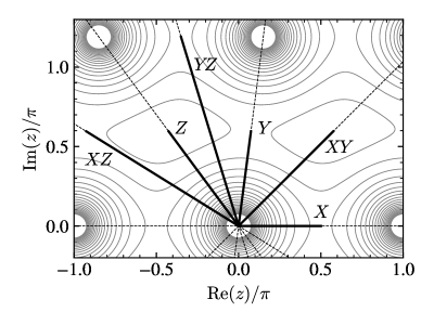
Figure 11: The continuum two-point function in the $z$-plane with modular parameter $\tau_{456}$, highlighting six axes along which we can easily measure the two-point function on our lattice.

We perform a simultaneous fit to Eq. 57 using lattice data for all six of these axes. The only fit parameter is an overall normalization factor. We can see in Fig. 12 that the lattice data is in excellent agreement with the continuum result.

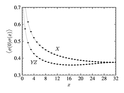
Figure 12: Two-point correlation function measured along the $X$ and $YZ$ axes shown in Fig. 11 for a triangular lattice with $\ell_{i}\propto\{4,5,6\}$ and $L=64$. The horizontal axis is the distance measured in lattice steps. The gray lines are the exact correlation function from Eq. 57 and the black points are lattice data.

5.2 The Critical Ising Model on $\mathbb{R}^{2}$: Finite-Size Scaling

In this section, we use the same lattice construction as in Sec. 5.1, but now we extract information about the continuum theory in an infinite plane via finite-size scaling. A similar analysis was done for an equilateral triangular lattice in [29]. Our formalism allows us to construct the lattice from triangles with any side lengths. Here, we again use triangles with $\ell_{i}\propto\{4,5,6\}$ because it is sufficiently different from an equilateral, isosceles, or right triangle and will show a clear difference between measurements along different triangle axes.

Again using critical couplings $\sinh 2K_{i}=\ell^{*}_{i}/\ell_{i}$, we measure the spin-spin correlation function along the six axes shown in Fig. 11. After scaling the step length for each axis appropriately, the correlation functions collapse onto a single curve at small separation, as shown in Fig. 13. At large separation, wraparound effects cause the correlation function behavior to depend slightly on which axis is being measured.

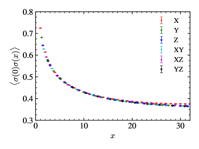
Figure 13: Spin-spin correlation function measured along each of the axes shown in Fig. 11 with distances scaled appropriately based on the lattice lengths $\ell_{i}$. Shown here for $\ell_{i}\propto\{4,5,6\}$.

We perform a finite-size scaling analysis [30, 31, 32] to extract the scaling exponent of the first $\mathbb{Z}_{2}$-odd primary operator, $\Delta_{\sigma}$. We measure the magnetic susceptibility $\chi=\langle m^{2}\rangle-\langle|m|\rangle^{2}$ where $m=\sum_{i}\sigma_{i}$ is the magnetization. On a finite lattice with characteristic size $L$, the magnetic susceptibility should scale as $\chi(L)\propto L^{2-2\Delta_{\sigma}}$. Fitting measurements on $L\times L$ triangular lattices for $L=8$ up to $L=256$, we find $\Delta_{\sigma}=0.12468(57)$, in excellent agreement with the exact continuum value $\Delta_{\sigma}=1/8$. Our fit is shown in Fig. 14.

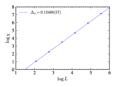
Figure 14: Finite-size dependence of magnetic susceptibility on a lattice with $\ell_{i}\propto\{4,5,6\}$.

5.3 Determination of Scaling via Radial Quantization

Here we present the lattice radial quantization method for measuring the correlation functions of conformal theories. In radial quantization, we perform a Weyl transformation

$$ds^{2}_{\text{flat}}=r^{2}[(d\log r)^{2}+d\Omega_{d-1}^{2}]\to ds^{2}_{\text{cyl.}}=dt^{2}+d\Omega_{d-1}^{2}$$ (58)

which takes the flat Euclidean manifold to a cylinder with spherical cross-section, $\mathbb{R}^{d}\to\mathbb{R}\times S^{d-1}$. The scale is fixed relative the radius of the sphere, which we have set to 1 by convention. In practice, this is very difficult in $d>2$ because there are no trivial lattice representations of $S^{d-1}$. In 2 dimensions however, we can simply reinterpret a typical periodic lattice as the manifold $\mathbb{R}\times S^{1}$ of radial quantization. The angular direction is inherently periodic, and therefore does not introduce unwanted wraparound effects. The periodic boundary conditions in the lattice radial direction still result in finite-size effects, but because of the Weyl transformation, equally-spaced lattice steps in the radial coordinate $t=\log r$ are actually exponentially spaced in the radial separation distance $r$. This means that conformal correlation functions, which have power-law scaling behavior, decay exponentially in lattice steps. Therefore wraparound effects are exponentially suppressed as the radial lattice size becomes large. This allows us to extract scaling dimensions for the operators of conformal theories using methods traditionally used to extract energies from operators in gapped theories.

The formalism presented in the previous sections allows us to simulate the radially quantized critical 2d Ising model with unequal lattice spacing in the radial and angular directions. For the results in this section we use a rectangular lattice

$$S=\frac{1}{2}\sum_{x,t}\left[K_{t}s_{t,x}s_{t+1,x}+K_{x}s_{t,x}s_{t,x+1}\right]$$ (59)

described in Eq. 50.

In the continuum, the exact two point function for the lowest $\mathbb{Z}_{2}$-odd primary operator $\sigma(t,\theta)$ on the infinite cylinder is

$$G(t,\theta)=\langle\sigma(t_{2},\theta_{2})\sigma(t_{1},\theta_{1})\rangle\propto\frac{1}{(\cosh t-\cos\theta)^{\Delta_{\sigma}}}$$ (60)

with $t=t_{1}-t_{2}$ and $\theta=\theta_{1}-\theta_{2}$ and $\Delta_{\sigma}=1/8$. On the lattice, we measure the Fourier coefficients of the two-point function, which we define as

$$C_{m}(t)=\sum_{x}\sigma(0)\sigma(t,x)\cos(2\pi mx/L_{x})$$ (61)

where $m$ is an integer and $(x,t)$ are the angular and radial separation in lattice units. We define a dimensionless “speed of light”, $c=2\pi a_{t}/L_{x}a_{x}$. Ignoring finite size effects, for large $t$ we expect a result with the form

$$C_{m}(t)\propto e^{-c\Delta_{\sigma}^{(m)}t}$$ (62)

where $\Delta_{\sigma}^{(0)}=\Delta_{\sigma}$ is the scaling exponent of the conformal primary operator and we expect the scaling exponents of the conformal descendant operators to be integer spaced in the continuum limit, i.e. $\Delta_{\sigma}^{(m)}\to\Delta_{\sigma}+m$ as $L\to\infty$. The $m=0$ coefficient is periodic in $t$ so we improve our fit by fitting to

$$C_{0}(t)\propto e^{-c\Delta_{\sigma}t}+e^{-c\Delta_{\sigma}(L_{t}-t)}\;.$$ (63)

We use an asymmetrical lattice with $L_{t}/L_{x}=8$ and $a_{t}/a_{x}=3/2$. Because we are using a rectangular lattice we can relate the lattice spacings to triangle side lengths via $a_{x}=\ell_{x}=\ell^{*}_{t}$ and $a_{t}=\ell_{t}=\ell^{*}_{x}$. The Ising coupling constants in the radial and angular directions are then given by $\sinh 2K_{t}=2/3$ and $\sinh 2K_{x}=3/2$, respectively. We note that the coupling constants for the diagonal links are zero and can therefore be neglected. On this lattice, finite-size effects from wraparound in the radial direction lead to corrections of order $\mathcal{O}(\exp(-c\Delta_{\sigma}L_{t})\simeq 10^{-5})$.

Some example fits are shown in Fig. 15. We use a Bayesian model-averaging procedure [33] to average over choices of the minimum $t$ value to include in each fit. We obtain our estimate for $\Delta_{\sigma}$ from the $m=0$ fit only. As shown in Fig. 16 on the left, we find that the descendant scaling exponents $\Delta_{\sigma}^{(m)}$ approach integer spacing as the lattice spacing goes to zero.

Finally, we measure $\Delta_{\sigma}(L_{x})$ on lattices with increasing $L_{x}$ to extrapolate to the continuum limit. We parameterize the finite-volume effects by fitting the finite lattice exponents to the form

$$\Delta_{\sigma}(L_{x})=\Delta_{\sigma}(\infty)+b/L_{x}^{\gamma}$$ (64)

which gives an infinite-volume scaling exponent of $\Delta_{\sigma}(\infty)=0.1249781(62)$ as shown in Fig. 16 on the right. For the other two fit parameters, we obtain $b=0.1245(22)$ and $\gamma=2.114(11)$.

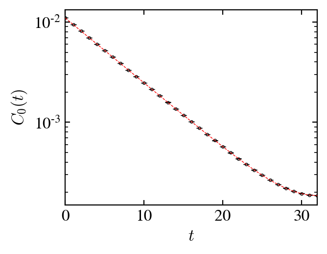
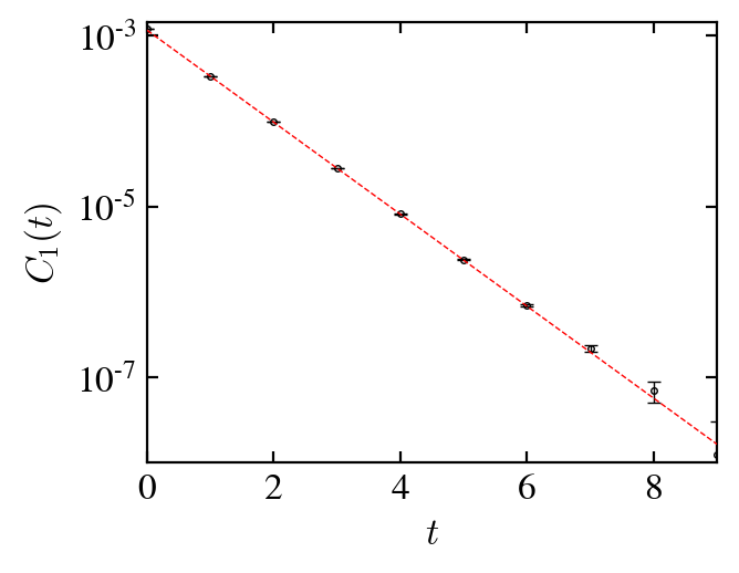
Figure 15: Examples of fits to Eq. 62 and 63 to extract the scaling behavior of the spin-spin two-point function in radial quantization. These plots are from an $8\times 64$ rectangular lattice with $a_{t}/a_{x}=3/2$.

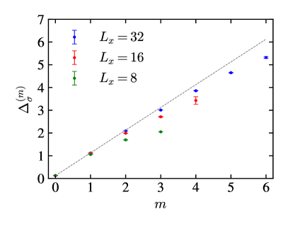
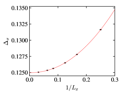
Figure 16: On the left the approximate integer spacing of descendant scaling exponents from rectangular lattices with $L_{t}=8L_{x}$ and $a_{t}/a_{x}=3/2$. The dashed line shows the continuum expectation of exact integer spacing from the primary, i.e. $\Delta_{\sigma}^{(m)}\to\Delta_{\sigma}+m$. On the right the continuum limit extrapolation of the scaling operator $\Delta_{\sigma}$. The red line is a fit to Eq. 64.

The asymmetric rectangular lattice has advantages which we will exploit in future efforts for $\mathbb{R}\times S^{d}$. Using finer lattice spacing in the radial direction $a_{t}\ll a_{x}$ may improve the extractions of conformal data for 2-point and 4-point functions. It is also interesting to study the finite temperature regime with fixed $\beta=a_{t}L_{t}\ll 1$. The expressions for the couplings $K_{x},K_{t}$ correspond to the Karsch coefficients [34] on an asymmetric lattice used in the extensive study of finite temperature studies for Lattice QCD. With the analytical form derived here, derivatives with respect to temperature $kT=1/\beta$ can be performed, leading to an efficient lattice application of the Ising thermodynamics formulated in Ref. [35]. Finally, to simulate the limit $a_{t}/a_{x}\to 0$, there are efficient continuous time worm-type Wolff cluster algorithms [36, 37]. As pointed out by Deng and Blöte[38] this is equivalent simulating the partition function $\operatorname{Tr}[\exp(-tH_{\text{QM}})]$ for the quantum spin Ising Hamiltonian,

$$H_{\text{QM}}=-\sum_{x,t}(\sigma^{1}_{x}+g^{2}\sigma^{3}_{x}\sigma^{3}_{x+1})$$ (65)

which has critical coupling is $g_{c}=1$. We expect to pursue this in the future with high-precision calculations.

6 Conclusion

We have shown that the 2d Ising model on a general uniform triangular grid maps to the $c=1/2$ minimal model on $\mathbb{R}^{2}$ if the lattice triangulation is given the appropriate affine transformation of the equilateral lattice. This we view as a simple and fortunately analytically soluble example of geometry emerging from a strong coupling quantum field theory at a second order critical surface. This affine lattice allowed us to simulate the toroidal geometry and take the continuum limit consistent with exact modular invariance.

We have used this example to suggest that there is a natural bridge between the projective geometry formalism for the CFT and the affine properties of finite elements on the simplicial complex and its Voronoi circumcenter dual. We note that the finite element method (FEM) provides a general solution for free conformal theories, defining the map from simplicial complex to continuum CFT on any smooth Riemann manifold in any dimension. While there is much more to consider in this geometric framework, it does suggest possible extensions to other strongly coupled CFTs.

First, in 2d flat space there are many exactly soluble theories which might provide additional examples for this map from lattice action parameters to continuum CFTs. Even beyond soluble models, numerical methods in higher dimensions could be performed to see if similar maps exist in a finite local parameter space, with the hope that the language of projective geometry will suggest an ansatz to test.

Second, based on our observation that affine transformations provide a general approach to mapping regular lattices in flat space locally to the tangent plane on the curved manifold to $\mathcal{O}(a^{2})$ in the lattice spacing $a$, it appears with preliminary numerical investigations that demanding a smooth $\mathcal{O}(a^{2})$ change in the affine connection between local tangent planes may enable the local determination of a lattice action in a finite parameter space to reach the continuum quantum field theory for the target geometry on the curved manifold. This would be a start at the quantum generalization of the QFE program to strong coupling CFTs. Initial efforts to apply this affine lattice framework to the tangent plane for radial quantization on $\mathbb{R}\times S^{1}$ and $\mathbb{R}\times S^{2}$ appear promising.

We acknowledge the challenges in both of these directions but with deeper insight into the connection between conformal geometry and the simplicial lattice calculus we believe some further progress appears likely.

References

- [1] Lars Onsager. Crystal statistics. I. A two-dimensional model with an order-disorder transition. Phys. Rev., 65:117–149, Feb 1944.
- [2] Jhih-Huang Li and Rémy Mahfouf. Conformal invariance in the quantum Ising model, 2021.
- [3] Richard C. Brower, Evan S. Weinberg, George T. Fleming, Andrew D. Gasbarro, Timothy G. Raben, and Chung-I Tan. Lattice Dirac Fermions on a Simplicial Riemannian Manifold. Phys. Rev., D95(11):114510, 2017.
- [4] Richard C. Brower, Michael Cheng, Evan S. Weinberg, George T. Fleming, Andrew D. Gasbarro, Timothy G. Raben, and Chung-I Tan. Lattice field theory on Riemann manifolds: Numerical tests for the 2-d Ising CFT on . Phys. Rev., D98(1):014502, 2018.
- [5] Richard C. Brower, George T. Fleming, Andrew D. Gasbarro, Dean Howarth, Timothy G. Raben, Chung-I Tan, and Evan S. Weinberg. Radial lattice quantization of 3d phi 4th field theory. Physical Review D, 104(9), Nov 2021.
- [6] Tullio Eugenio Regge. General relativity without coordinates. Il Nuovo Cimento (1955-1965), 19:558–571, 1961.
- [7] Muhammad Asaduzzaman and Simon Catterall. Euclidean Dynamical Triangulations Revisited. 7 2022.
- [8] Charles Nash and Denjoe O’Connor. Modular invariance, lattice field theories, and finite size corrections. Annals of Physics, 273(1):72–98, 1999.
- [9] D. V. Yur’ev. Complex projective geometry and quantum projective field theory. Theoretical and Mathematical Physics, 101(3):1387–1403, 1994.
- [10] Richard C. Brower, Cameron V. Cogburn, and Evan Owen. Hyperbolic lattice for scalar field theory in AdS3. Phys. Rev. D, 105(11):114503, 2022.
- [11] NH Christ, R Friedberg, and TD Lee. Random lattice field theory: General formulation. Nuclear Physics B, 202(1):89–125, 1982.
- [12] NH Christ, R Friedberg, and TD Lee. Gauge theory on a random lattice. Nuclear Physics B, 210(3):310–336, 1982.
- [13] NH Christ, R Friedberg, and TD Lee. Weights of links and plaquettes in a random lattice. Nuclear Physics B, 210(3):337–346, 1982.
- [14] G. E. Sobczyk. Simplicial calculus with Geometric Algebra, page 279–292. Springer Netherlands, Dordrecht, 1992.
- [15] Douglas Lundholm and Lars Svensson. Clifford algebra, geometric algebra, and applications, 2009.
- [16] Giuseppe Mussardo. Statistical field theory: an introduction to exactly solved models in statistical physics. Oxford Univ. Press, New York, NY, 2010.
- [17] R.M.F. Houtappel. Order-disorder in hexagonal lattices. Physica, 16(5):425–455, 1950.
- [18] H. A. Kramers and G. H. Wannier. Statistics of the two-dimensional ferromagnet. Part I. Phys. Rev., 60:252–262, Aug 1941.
- [19] Robert H. Swendsen and Jian-Sheng Wang. Nonuniversal critical dynamics in Monte Carlo simulations. Phys. Rev. Lett., 58:86–88, Jan 1987.
- [20] Mark Kac and John C Ward. A combinatorial solution of the two-dimensional Ising model. Physical Review, 88(6):1332, 1952.
- [21] Ulli Wolff. Ising model as Wilson-Majorana Fermions. Nucl. Phys. B, 955:115061, 2020.
- [22] R. Brower, R. Giles, and G. Maturana. Link fermions in euclidean lattice gauge theory. Phys. Rev. D, 29:704–715, Feb 1984.
- [23] P. Ginsparg. Matrix models of 2d gravity. 1991.
- [24] Blaise Pascal. Essay pour les conique. (facsimile) Niedersächsiche Landesbibliothek, Gottfried Wilhelm Leibniz Bibliothek, 1640.
- [25] S. M. Catterall. Critical Z(N) symmetric spin models in strip geometries: a Monte Carlo study. Phys. Lett. B, 231:141–146, 1989.
- [26] Nicholas Metropolis, Arianna W. Rosenbluth, Marshall N. Rosenbluth, Augusta H. Teller, and Edward Teller. Equation of state calculations by fast computing machines. Journal of Chemical Physics, 21(6):1087–1092, 1953.
- [27] Ulli Wolff. Collective Monte Carlo updating for spin systems. Phys. Rev. Lett., 62:361–364, Jan 1989.
- [28] P. Di Francesco, H. Saleur, and J.B. Zuber. Critical Ising correlation functions in the plane and on the torus. Nuclear Physics B, 290:527–581, 1987.
- [29] Luo Zhi-Huan, Loan Mushtaq, Liu Yan, and Lin Jian-Rong. Critical behaviour of the ferromagnetic Ising model on a triangular lattice. Chinese physics B, 18(7):2696–2702, 2009.
- [30] Michael E. Fisher and Michael N. Barber. Scaling theory for finite-size effects in the critical region. Physical review letters, 28(23):1516–1519, 1972.
- [31] D. P. Landau. Finite-size behavior of the simple-cubic Ising lattice. Phys. Rev. B, 14:255–262, Jul 1976.
- [32] K. Binder. Finite size scaling analysis of Ising model block distribution functions. Z. Phys. B, 43:119–140, 1981.
- [33] William I. Jay and Ethan T. Neil. Bayesian model averaging for analysis of lattice field theory results. Physical Review D, 103(11), Jun 2021.
- [34] Frithjof Karsch. SU(N) gauge theory couplings on asymmetric lattices. Nuclear Physics B, 205(2):285–300, 1982.
- [35] Luca Delacrétaz, Andrew Liam Fitzpatrick, Emanuel Katz, and Matthew Walters. Thermalization and hydrodynamics of two-dimensional quantum field theories. SciPost Physics, 12(4), apr 2022.
- [36] Henk W. J. Blöte and Youjin Deng. Cluster Monte Carlo simulation of the transverse Ising model. Phys. Rev. E, 66:066110, Dec 2002.
- [37] Youjin Deng and Henk W. J. Blöte. Anisotropic limit of the bond-percolation model and conformal invariance in curved geometries. Phys. Rev. E, 69:066129, Jun 2004.
- [38] Youjin Deng and Henk WJ Blöte. Conformal invariance and the Ising model on a spheroid. Physical Review E, 67(3):036107, 2003.