Bayesian Neural Networks for Geothermal Resource Assessment:
Prediction with Uncertainty

Abstract

We consider the application of machine learning to the evaluation of geothermal resource potential. A supervised learning problem is defined where maps of 10 geological and geophysical features within the state of Nevada, USA are used to define geothermal potential across a broad region. We have available a relatively small set of positive training sites (known resources or active power plants) and negative training sites (known drill sites with unsuitable geothermal conditions) and use these to constrain and optimize artificial neural networks for this classification task. The main objective is to predict the geothermal resource potential at unknown sites within a large geographic area where the defining features are known. These predictions could be used to target promising areas for further detailed investigations. We describe the evolution of our work from defining a specific neural network architecture to training and optimization trials. Upon analysis we expose the inevitable problems of model variability and resulting prediction uncertainty. Finally, to address these problems we apply the concept of Bayesian neural networks, a heuristic approach to regularization in network training, and make use of the practical interpretation of the formal uncertainty measures they provide.

Copyright © 2023 Stephen R. Brown

1 Introduction

Many problems in Earth sciences concerning the environment, energy, and natural hazards involve taking a set of observations on a map and making predictions about some unknown or unseen characteristic: such as predicting a numerical quantity, recognizing a particular structure or category, or building a new classification or taxonomy. Applications of practical importance are energy and mineral prospecting and resource assessment, location of buried objects of specific types such as land mines and tunnels, prediction of pathways for migration of groundwater contaminants, or searching for anomalies within a complex background as in security monitoring, to name a few.

To tackle these problems, one is tempted to bring to bear the recent developments and successes in artificial intelligence (AI) and its popular implementations known as machine learning, especially artificial neural networks. However, the nature of the data in many Earth science applications makes direct application of many successful AI methods difficult.

First, our problems generally have a paucity of examples with known labels (training sites) for problems for which we would hope to apply supervised learning methods. Many problems in computer vision such as facial recognition, autonomous driving, image recognition, etc., have many tens to perhaps hundreds of thousands of labeled examples from which to train, develop, and test deep network algorithms and architectures. While some geoscience problems such as hyper-spectral satellite imaging have as much training data (e.g. Zhu,, 2017), many have fewer than a hundred labeled examples. Another consideration is the nature of the data itself. Input features carrying important information for the regression or classification will necessarily be a mixture of numerical values (real numbers such as temperature, distance from a geologic fault, or gravity anomaly), categorical variables (mineral assemblages or rock type descriptions), and ordinal variables (i.e., ranked as this is bigger than that, but with no scaling). Geologic data will commonly be indexed to maps and thus are related spatially to other features. These data, however, may not have the same resolution nor the same degree of certainty. Finally, there are physical principles, variably understood ahead of time, which point to reasonable relationships between features and labels. Incorporating such “expert” knowledge into the hypotheses is important, especially to counter the problem of a small number of examples and to ensure proper weighting of the uncertainty of various data sources.

Generally, supervised machine learning uses two sources of knowledge: (1) labeled data pairs (features, labels) and (2) hand-engineered features, network architecture, and other components. For the cases of relatively few labeled feature-outcome pairs, we often use more hand engineering and/or specialized algorithms. For the cases having a large number of training examples, we can generally apply simpler algorithms and less hand engineering. For small numbers of training data, hand engineering is commonly the most efficient way to improve learning performance.

One would like to strike a balance between the ideal of feeding large numbers of features into a network and letting the algorithm determine the relationships and, on the other extreme, engineering the complete hypothesis and algorithm by hand. The former, while unbiased and allowing the data to speak for themselves, can be prone to overfitting and for this application is perhaps at best inefficient or at worst intractable. The latter runs the risk of extreme bias leading to under-fitting such that important links among features will never be recognized. Also, the algorithms developed in the hand-engineered approach may not be extensible to new data types nor to new areas of application. For these reasons, in this paper we use supervised machine learning techniques and allow the training data examples to determine the model details as much as possible.

Here, we consider the problem of prospecting and evaluation of geothermal energy resources. We take as a case study the evaluation of potential blind geothermal systems in the U.S. state of Nevada studied previously in the Nevada Geothermal Play Fairway Project (Faulds et al.,, 2013, 2015, 2017, 2018, 2019) (see Figure 1). We proceed by revisiting the results from this previous study and re-analyzing the accompanying data set using machine learning methods. In so doing, we gain experience in bringing machine learning principles to bear on this important class of Earth science problems. In the end we show that by using a Bayesian approach we can naturally include model uncertainty and provide a way not only to predict resource potential but to also give measures of confidence or reliability.

2 Problem Setting

The Great Basin region (Figure 1) is a world-class geothermal province with more than 1,200 MWe of installed capacity from 28 power plants. Studies indicate far greater potential for both conventional hydrothermal and enhanced geothermal systems (EGS) in the region (Williams et al.,, 2009).

Because most geothermal systems in the Great Basin are controlled by Quaternary normal faults, they generally reside near the margins of actively subsiding basins. Thus, upwelling fluids along faults commonly flow into permeable subsurface sediments in the basin and do not reach the surface directly along the fault. Outflow from these upwellings may emanate many kilometers away from the deeper source or remain blind with no surface manifestations (Richards and Blackwell,, 2002). Blind systems are thought to comprise the majority of geothermal resources in the region (Coolbaugh et al.,, 2007). Thus, techniques are needed to both identify the structural settings enhancing permeability and to determine which areas may host subsurface hydrothermal fluid flow.

Geothermal play fairway analysis (PFA) is a concept adapted from the petroleum industry (Doust,, 2010) that aims to improve the efficiency and success rate of geothermal exploration and drilling by integration of geologic, geophysical, and geochemical parameters indicative of geothermal activity. A prior demonstration project (Faulds et al.,, 2017) focused on defining geothermal play fairways, generating detailed geothermal potential maps for approximately 1/3 of Nevada, and facilitating discovery of blind geothermal fields. The Nevada Geothermal Play Fairway Project incorporated around 10 geologic, geophysical, and geochemical parameters indicative of geothermal activity. It led to discovery of two new geothermal systems (Craig,, 2018; Faulds et al.,, 2018, 2019; Craig et al.,, 2021). The PFA leveraged logistic regression, weights of evidence, and other statistical measures as a type of machine learning technique. A set of features, each gauged by a perceived weight of influence, were combined to estimate geothermal potential. However, key limitations and challenges affected the PFA, including estimating weights of influence for parameters, limitations of some data sets, and a limited number of training sites. We have been building upon the original Nevada Geothermal Play Fairway Project of Faulds et al., (2017, 2018) to include principles and techniques of machine learning (Faulds et al.,, 2020; Brown et al.,, 2020; Smith,, 2021). In this paper, we focus on the application of stochastic variational Bayes neural networks to the problem of geothermal resource assessment.

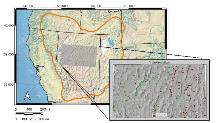
Figure 1: The Nevada Play Fairway Study Area (gray) is shown within the Great Basin Region (orange). The inset detail shows the locations of positive and negative training sites within the study area.

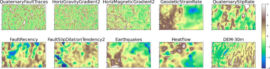
Figure 2: Geological and geophysical numerical feature maps used in this study. These maps were derived and updated from the original PFA study (Faulds et al.,, 2018, 2020).

3 Classification with Fully Connected Neural Networks

3.1 Define a Supervised Learning Problem

Our problem is constrained by data sets developed for the original Nevada Geothermal Play Fairway Project. Some of these data were further improved and made available for our use by DeAngelo et al., (2021). Each of the geological and geophysical features shown in Figure 2 are presented as geo-referenced maps and are known everywhere on a $250\times 250$ meter pixel grid throughout the study area. At certain geographic locations there are benchmarks, where it is known whether or not a geothermal potential exists, i.e., an existing power plant or definitive positive or negative drilling results. Training data include 83 positive sites from known geothermal systems ($\geq 39^{\circ}$C) and 62 negative sites from wells that that showed negative geothermal development potential, most of which were selected from relatively deep and cool wells associated with oil and gas exploration. The criteria used to select these training sites is described by Smith, (2021). Together these positive and negative sites as shown in Figure 1 comprise the “labels” used in training of the algorithms.

A supervised learning algorithm is trained by repeatedly presenting it with these labeled examples and updating the model parameters until the predictions of the model match the training data satisfactorily. Ultimately the trained model would then be used to predict the probability that non-benchmark sites throughout the study region are positive geothermal prospects.

In what follows we provide the mathematical foundation for the supervised learning classification problem using artificial neural networks (ANN). This motivates further descriptions of the construction and training of the models, helps develop insight into the effects of hyperparameter choices, and most importantly lends clear meaning to the predictions.

3.2 Mathematical Formulation for ANN

3.2.1 Classification Problem

We assume the existence of a population of potential geothermal sites, each associated with a pair $(\mathbf{x},y)$, where the vector $\mathbf{x}$ contains numerical measurements (features) acquired at the site, and where the Boolean variable $y\in\{0,1\}$ indicates which of two classes the site belongs to. We take $y=1$ to mean the site is a positive geothermal prospect and $y=0$ to mean it is a negative prospect. The geothermal classification problem is to devise a function that maps the feature vector $\mathbf{x}$ to the class $y$.

A statistical approach to this problem treats $y$ as a random variable characterized by a probability mass function (PMF), dependent on $\mathbf{x}$. We denote this PMF as $f(y\kern 0.74997pt|\kern 0.74997pt\mathbf{x})$, showing the $\mathbf{x}$-dependence as conditioning even though our approach will not consider the randomness of $\mathbf{x}$. The PMF of $y$ takes values only for $y=0$ and $y=1$, with $f(0\kern 0.74997pt|\kern 0.74997pt\mathbf{x})$ being the probability that $y=0$ for a site with feature vector $\mathbf{x}$, and with $f(1\kern 0.74997pt|\kern 0.74997pt\mathbf{x})=1-f(0\kern 0.74997pt|\kern 0.74997pt\mathbf{x})$.

Adopting the point of view of Bishop, (2006) and others, we can break the classification problem into two subproblems. The first, which is the topic of this paper, is to infer, or learn, $f(y\kern 0.74997pt|\kern 0.74997pt\mathbf{x})$ from training data. Given the inferred $f(y\kern 0.74997pt|\kern 0.74997pt\mathbf{x})$, the second subproblem is to decide whether $y=0$ or $y=1$ for a new site of interest having feature vector $\mathbf{x}$. A simple decision rule would be to classify the site as $y=1$ if $f(1\kern 0.74997pt|\kern 0.74997pt\mathbf{x})>f(0\kern 0.74997pt|\kern 0.74997pt\mathbf{x})$ and as $y=0$ otherwise. More complex rules ensue from consideration of issues such as misclassification costs, opportunity loss, and availability of prior information about $y$. These issues fall within the domain of decision theory and are not addressed in this paper.

3.2.2 Statistical Model

We attribute the stochastic nature of $y$ to the notion of random selection, whereby a site we wish to classify is considered a random draw from a population of similar sites, a proportion $p$ of which is labeled $y=1$ and the remainder labeled $y=0$. For a given value of $p$, the PMF of $y$ for the selected site is the Bernoulli distribution, given by

$$f(y\kern 0.74997pt|\kern 0.74997ptp) =p^{y}\kern 0.74997pt(1-p)^{1-y}$$ (1)

or, enumerating,

$$f(y\kern 0.74997pt|\kern 0.74997ptp) =\begin{cases}p&\text{for }y=1\\ 1-p&\text{for }y=0.\end{cases}$$ (2)

The use of conditioning notation to indicate dependence on $p$ is not gratuitous in this case, as we will later treat $p$ as a random variable. Implicit in the Bernoulli model is that the dependence of $y$ on $\mathbf{x}$ arises solely from the dependence of $p$ on $\mathbf{x}$, expressed as

$$f(y\kern 0.74997pt|\kern 0.74997ptp,\mathbf{x}) =f(y\kern 0.74997pt|\kern 0.74997ptp).$$ (3)

Of importance to applications in decision theory we remark that, given (2), it is appropriate to refer to the parameter $p$ as a probability, rather than a proportion of the population. Further, in the interpretation that the case $y=1$ is considered a “successful” draw, it is appropriate to consider $p$ to be the probability of success.

The PMF $f(y\kern 0.74997pt|\kern 0.74997pt\mathbf{x})$ is determined by the Bernoulli model in conjunction with a model for the dependence of $p$ on $\mathbf{x}$. The latter model must be inferred from training data and, since a training data set is inherently limited, prior constraints on the relationship between $p$ and $\mathbf{x}$. Here, we constrain this relationship by taking $p$ to be a specified function of $\mathbf{x}$ and a vector of parameters, ${\bm{\gamma}}$, assumed to be independent of $\mathbf{x}$:

$$p =P(\mathbf{x},{\bm{\gamma}}).$$ (4)

We construct the function $P$ as follows. First, to enforce $0\leq p\leq 1$, we let $p$ be the logistic function of an unconstrained variable $z$:

$$p =\frac{1}{1+\exp\big{(}-z)}.$$ (5)

We see that $z=-\infty$, $0$, $\infty$ map to $p=0$, 1/2, 1, respectively. Second, we let $z$ be a specified function of $\mathbf{x}$ and ${\bm{\gamma}}$, which we express as

$$z =Z(\mathbf{x},{\bm{\gamma}}).$$ (6)

The method of logistic regression (e.g. Goodfellow et al.,, 2016, Chapter 1), for example, takes ${\bm{\gamma}}=(b,\mathbf{w})$ and $Z$ as the linear function

$$Z(\mathbf{x},{\bm{\gamma}}) =b+\mathbf{w}^{\mathit{T}}\mathbf{x}$$ (7)

with $b$ a bias parameter and $\mathbf{w}$ a vector of feature weights. In general, combining Equations (5) and (6) defines the function $P$ in (4).

Our approach generalizes logistic regression by taking $Z$ to be a nonlinear function of $\mathbf{x}$, implemented as a multilayer neural network with an input node for each observed feature (component of $\mathbf{x}$) and a single output node corresponding to $z$. The components of ${\bm{\gamma}}$ are the biases assigned to the nodes in each layer and the weights assigned to connections between the nodes of adjacent layers. Since the logistic function in (5) conforms to the activation functions typically used in neural networks, it is convenient to, and we hereinafter do, take the function $P$ itself to be the neural network, with (5) applied at the output node to yield $p$.

Combining Equations (1) and (4), we obtain an expression for the PMF of $y$, now dependent on ${\bm{\gamma}}$ as well as $\mathbf{x}$:

$$f(y\kern 0.74997pt|\kern 0.74997pt\mathbf{x},{\bm{\gamma}}) =P(\mathbf{x},{\bm{\gamma}})^{y}\kern 0.74997pt\big{(}1-P(\mathbf{x},{\bm{\gamma}})\big{)}^{1-y}.$$ (8)

The inference of $f(y\kern 0.74997pt|\kern 0.74997pt\mathbf{x})$ reduces to the inference of the parameter vector ${\bm{\gamma}}$.

3.2.3 Training the Neural Network

For a fixed value of ${\bm{\gamma}}$, the function $P$ represents a conventional, deterministic neural network that predicts, for arbitrary $\mathbf{x}$, a specific value of $p$ (via Equation (4)) as well as the PMF of $y$ (via (8)). A suitable value of ${\bm{\gamma}}$ to use for these predictions results from applying machine learning to a set of training data obtained from sites with known class. Given $N$ such sites, we denote the training data set $(\mathbf{x}_{i},y_{i})$, $i=1$, …, $N$, or, for brevity, the pair of tuples $(X,Y)$ defined as

$$X =(\mathbf{x}_{1},\mathbf{x}_{2},\ldots,\mathbf{x}_{N})$$ (9)

$$Y =(y_{1},y_{2},\ldots,y_{N}).$$ (10)

A standard approach in machine learning is to set ${\bm{\gamma}}$ to the value that maximizes the likelihood of the training data set, defined as $f(Y\kern 0.74997pt|\kern 0.74997ptX,{\bm{\gamma}})$ and, considered as a function of ${\bm{\gamma}}$, known as the likelihood function. With $Y$ being known, this is a supervised learning approach and, given our explicit model parameterization, reduces to statistical regression.

We assume the $y_{i}$ are statistically independent, implying in conjunction with Equation (8)

$$f(Y\kern 0.74997pt|\kern 0.74997ptX,{\bm{\gamma}}) =\prod_{i=1}^{N}P(\mathbf{x}_{i},{\bm{\gamma}})^{y_{i}}\kern 0.74997pt\big{(}1-P(\mathbf{x}_{i},{\bm{\gamma}})\big{)}^{1-y_{i}}.$$ (11)

In numerical applications it is convenient to deal with the negative logarithm of likelihood, which we show as a function, ${\cal L}$, of ${\bm{\gamma}}$ and the training data. Equation (11) yields this as

$${\cal L}({\bm{\gamma}};X,Y) \equiv-\log f(Y\kern 0.74997pt|\kern 0.74997ptX,{\bm{\gamma}})$$

$$=-\sum_{i=1}^{N}y_{i}\kern 0.74997pt\log P(\mathbf{x}_{i},{\bm{\gamma}})-\sum_{i=1}^{N}(1-y_{i})\kern 0.74997pt\log\big{(}1-P(\mathbf{x}_{i},{\bm{\gamma}})\big{)}$$

$$=-\sum_{i=1\atop y_{i}=1}^{N}\log P(\mathbf{x}_{i},{\bm{\gamma}})-\sum_{i=1\atop y_{i}=0}^{N}\log\big{(}1-P(\mathbf{x}_{i},{\bm{\gamma}})\big{)}$$ (12)

where the summations in the latter expression separate the positive training sites ($y_{i}$=1) from the negative ones. The maximum-likelihood value of ${\bm{\gamma}}$ can then be stated as

$${\bm{\gamma}}_{\mathsf{ML}} =\arg\min_{\bm{\gamma}}{\cal L}({\bm{\gamma}};X,Y).$$ (13)

Our implementation of deterministic neural networks calculates ${\bm{\gamma}}_{\mathsf{ML}}$ by applying a gradient descent procedure to minimize ${\cal L}$, using the well-known back-propagation technique (e.g. Goodfellow et al.,, 2016, Chapter 6) to perform gradient computations.

3.2.4 Regularization of Network Training

Equation (13) defines ${\bm{\gamma}}_{\mathsf{ML}}$ as the value of ${\bm{\gamma}}$ that best predicts, or fits, the training data set. This means that, overall, $P(\mathbf{x}_{i},{\bm{\gamma}}_{\mathsf{ML}})$ is as close as possible to one for positive training sites and to zero for negative training sites. Being optimal in this sense, however, does not guarantee that ${\bm{\gamma}}_{\mathsf{ML}}$ will successfully predict the class of new sites. The predictive value of ${\bm{\gamma}}_{\mathsf{ML}}$ will ultimately depend on two factors: how well the parameter vector ${\bm{\gamma}}$ characterizes the relationship between $p$ and $\mathbf{x}$, for relevant values of $\mathbf{x}$; and how well the training data set constrains ${\bm{\gamma}}$. When ${\bm{\gamma}}$ is not well constrained ${\bm{\gamma}}_{\mathsf{ML}}$ will be vulnerable to “overfitting” the training data and will yield poor predictions for new values of the feature vector $\mathbf{x}$.

The classical remedy for overfitting in machine learning, and inverse problems in general, is regularization. In our context, this means relaxing the maximum-likelihood criterion in Equation (13) with auxiliary conditions on ${\bm{\gamma}}$. A standard technique is to augment ${\cal L}$ with a penalty term and seek the value of ${\bm{\gamma}}$ that minimizes the augmented function.

3.3 Neural Network Architecture

The original Nevada Geothermal Play Fairway Project as applied to the Great Basin devised a computation graph grounded in statistical analyses for estimation of geothermal resource potential in the region (refer to Figure 3 of Faulds et al.,, 2018). Specific geological and geophysical features were chosen as they were thought to indicate essential aspects of permeability and heat sources. These features were combined algebraically in a method conditioned by the knowledge of known resource benchmark sites to calculate the “fairway,” a number scaled to indicate a region-wide degree of the geothermal potential (Figure 1 of Faulds et al.,, 2018).

We recognized that this computation graph is a feed-forward network, in effect a highly engineered neural network where the nodes are connected in a very specific way. In this paper we build upon this previous work and formulate the problem using standard artificial neural network techniques. We want to build upon the experience gained in the previous project of Faulds et al., (2018), therefore we use the same feature data sets with enhancements (DeAngelo et al.,, 2021) allowing us to use their fairway map as a point of comparison with our results.

We first must decide on the specific fully connected network architecture to use. In particular we must decide upon the number of neurons per layer and the number of layers and choose values of any additional hyperparameters the algorithm requires. A scoping study was done to find an optimum set of model parameters. A “best” network was sought using genetic algorithm methods (specifically the Python implementation “DEAP” of Fortin et al., (2012)) to efficiently search through various network structures and combinations of hyperparameters. The suitability of each candidate was gauged through performance metrics that emphasize the trade-off between data over-fitting and model complexity (the Akaike Information Criterion and the Bayesian Information Criterion described in Fabozzi et al., (2014)). The genetic algorithm built a population of networks, evaluated each one, modified them, and kept the most suitable individuals. In the end we found that there are certainly unsuitable networks to use. Those networks too simple, such as one with only one hidden layer only or a network mimicking the engineered computation graph used in the original Nevada Geothermal Play Fairway Project (Figure 3 of Faulds et al.,, 2018) or those networks with very narrow yet deep configurations (such as 8 layers of 4 neurons each, for example) do not train consistently nor generalize well to new examples not seen during training. At the other extreme, those networks both wide and deep (such as 8 layers of 16 neurons each, for example) are also unsuitable since these have large numbers of parameters, overfit or memorize the training data, and must be heavily regularized in order to generalize. There are, however, many networks in between which seem to be equally suitable as they train consistently well, can fit our the data to reasonable accuracy and can be easily kept from overfitting with some form of regularization. The network we settled upon for our studies is shown in Figure 3 with two hidden layers of 16 neurons each. The number of neurons was chosen to be just more than the anticipated maximum number of features to be available for study, thinking that it would allow all conceivable interconnections among the features in determining the outcome. The single output neuron indicates the probability of a positive site.

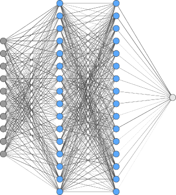
Figure 3: Fully connected neural network used for this study. The vertical set of dark gray circles on the left represents the 10 input features, the light gray circle on the right represents the output neuron (prediction) and the vertically-aligned blue circles in the center represent the 16 neurons in each of the two hidden layers. Each shaded gray line indicates that each interconnection (combination of weights and biases) is unique.

3.4 Implementation

We provide a brief description of the implementation of a basic fully connected neural network. As we follow standard methods in the field of machine learning, we will only highlight those algorithm components helpful for a comparison of this network to the probabilistic networks employed later.

We read from left to right in the graphical representation of the network in Figure 3. The network consists of a set of neurons organized into layers. The set of input features are combined linearly at each neuron and then passed through a nonlinear activation function. The output of each activation function becomes a new internal feature for the next layer of neurons. This computation is applied, layer upon layer, until the final neurons are reached. The outputs of the final layer represent the prediction. Such a forward pass through the network is described in pseudo code as Algorithm 1. The forward-pass algorithm is at the heart of both training of the network and its subsequent use for prediction.

Algorithm 1 Forward pass through a neural network computing $p=P(\mathbf{x},{\bm{\gamma}})$, with ${\bm{\gamma}}=(\mathbf{W},\mathbf{b})$ from Equation (4). Inputs are given as a column vector $\mathbf{x}$ containing all of the input features. For each neuron we also define a column vector of weights $\mathbf{w}$, each component of which corresponds to a specific input to that neuron. Expanding from the simple logistic regression case to layers of many neurons, we now represent each layer by the weight matrix $\mathbf{W}$ containing the horizontally stacked weight vectors $\mathbf{w}$ for all neurons in that layer. Once transposed, each row of $\mathbf{W}^{T}$ represents a neuron and the elements of each column represent the weights multiplying the output of each neuron in the previous layer. A column vector $\mathbf{b}$ contains the biases for all neurons. Each step represents a set of linear combinations of the outputs from the previous layer ($\bm{z}$) represented as a matrix algebra operation followed by the application of a nonlinear activation function $g(\bm{z})$, possibly unique to each layer. The network returns the predictions as the activations from the final layer. 1:procedure ForwardPass($\mathbf{x},\mathbf{W},\mathbf{b}$) 2:     $\mathbf{a}^{[0]}\leftarrow\mathbf{x}$ $\triangleright$ begin with the input features 3:     for $l$ in layers do $\triangleright$ loop over all layers 4:         $\bm{z}^{[l]}\leftarrow\mathbf{W}^{[l]\textrm{T}}\mathbf{a}^{[l-1]}+\mathbf{b}^{[l]}$ $\triangleright$ linear combinations of previous layer’s outputs 5:         $\mathbf{a}^{[l]}\leftarrow g^{[l]}(\bm{z}^{[l]})$ $\triangleright$ apply activation function       6:     $p\leftarrow\mathbf{a}^{[\textrm{final}]}$ $\triangleright$ final layer’s activation is the probability 7:     return $p$ $\triangleright$ return the prediction

The main steps in training a neural network are summarized in pseudo code in Algorithm 2. Briefly, to train the network first any model hyperparameters such as regularization parameters are chosen. Then the trainable model parameters (the weights and biases) are initialized to random values. A set of training examples is repeatedly presented to the algorithm. The training features are used in Algorithm 1 to produce an interim prediction. This prediction is then compared to the known outcome for the example and the misfit between them, known as the loss or the cost, is used in an optimizer for and incremental update of the model parameters. This training loop proceeds until a satisfactory solution is found and the final model parameters are saved. The training process is monitored through learning curves consisting of both the evolution of the loss and the evolution of the predictive accuracy. These training metrics are reported each epoch. An epoch counts one forward pass of every training example through the network. Some training examples are held out and used to test the ability of the network to generalize to unseen examples.

Algorithm 2 Training a neural network. A set of example features $\bm{X}$ and corresponding labels $\bm{Y}$ are used to iteratively improve the model weights $\mathbf{w}$ and biases $\mathbf{b}$ from their initial random values by comparing model predictions of the labels $\hat{y}$ to the true labels $y$ through a cost function. See text for further explanation. 1:choice of model hyperparameters 2:randomly initialized weights and biases 3:procedure Train($\bm{X},\bm{Y}$) $\triangleright$ input all training example features and labels 4:     repeat 5:         $\mathcal{L}\leftarrow 0$ $\triangleright$ set cost to 0 6:         for all $\mathbf{x},y$ in $\bm{X}$, $\bm{Y}$ do $\triangleright$ consider each training example 7:              $\hat{y}\leftarrow\textrm{ForwardPass}(\mathbf{x},\mathbf{W},\mathbf{b})$ $\triangleright$ predict with a forward pass through the network 8:              $\mathcal{L}\leftarrow\mathcal{L}+\textrm{Cost}(y,\hat{y})$ $\triangleright$ sum the cost of misfit to all data           9:         $\mathbf{W},\mathbf{b}\leftarrow\textrm{Update}(\textrm{Optimizer},\mathcal{L})$ $\triangleright$ update model based on total cost 10:     until model is optimized 11:     return $\mathbf{w},\mathbf{b}$ $\triangleright$ return optimized weights and biases

Algorithms 1 and 2 were coded in the Python programming language and the neural networks were implemented using the PyTorch imperative deep learning library (Paszke et al.,, 2019) on a Linux computer with an integral graphics processing unit (GPU).

In the examples provided below, in lieu of the penalty approach for regularization mentioned in Section 3.2.4 , we regularized the learning problem with procedures provided with the PyTorch software. In particular, we invoked the built-in “dropout” or “weight decay ” mechanisms (e.g. Goodfellow et al.,, 2016; Paszke et al.,, 2019), applied within the gradient descent iteration, both of which essentially detect and remove (set to zero) poorly constrained components of ${\bm{\gamma}}$.

To apply this model to the geothermal resource potential problem, the 10 feature maps from the Nevada Geothermal Play Fairway Project (Figure 2) were initially reformatted into a flattened table where each column represents the feature values, and these are organized row-wise keyed to the geographic location on the map. The features were then prescaled so that they each have a mean value of 0.0 and a standard deviation of 1.0.

The features of the benchmark sites (Figure 1 inset) were extracted from this table for training and testing. There are 62 positive sites and 84 negative sites in this database. The training data set was balanced by randomly selecting 62 of the negative sites from the original 84 examples. We found that with this small number of training data the optimization was found to be erratic in each training cycle and from one trial to the next. Therefore, the data set was augmented for numerical stability by adding the 4 nearest neighbors on the map to each true benchmark. These 620 examples in total provided stability and repeatability to the training process. The augmented benchmarks were randomly split into 67% training examples and 33% testing examples. The models were then trained in batches using back propagation and the Adam optimizer (e.g. Goodfellow et al.,, 2016, Chapter 8).

The learning curves, including the loss versus epoch and the training and testing accuracy vs epoch, were used to gauge the process and used to help choose the regularization hyperparameters to prevent overfitting as seen by a large discrepancy between training and testing accuracy. Both dropout and weight decay were explored as regularizing methods.

Finally, once a model is successfully trained and tested and deemed suitable, the probability of finding new positive sites in the study area is predicted by feeding the features forward through the model at each remaining geographic location (pixels). From these predictions a geothermal resource map can be produced analogous to the original Nevada Geothermal Play Fairway Project map (Figure 1 of Faulds et al.,, 2018).

3.5 Results

When we perform this training and prediction exercise and produce typical outcomes for the resource maps, we notice two related issues requiring further consideration. First, there is the general issue of confidence in the predictions driven by the need to choose additional model heuristics related to regularization. The goal of this work is to produce practical resource maps guiding geothermal exploration and drilling. Confidence in the map is a key input to this decision making process. A second and related issue is that even once all model parameters are fixed, there is still a noticeable degree of variability in the outcomes, especially in the details of the maps produced by prediction from multiple optimizations of the model. This variability must be understood and reconciled for the results to be most useful. Below, we illustrate these issues with examples and then propose a means to incorporate them into our understanding.

3.5.1 Discussion of confidence in predictions

A hidden aspect in all neural network models is the ability and need to regularize the behavior in training in order to reduce over-fitting to the training examples and ensure generalization to unseen examples studied during the testing stage. In our network we have some choices in this regard, first is to restrict any one weight or bias from becoming too large and dominating the solution. This in PyTorch is known as “weight decay.” Another method we can use, either separately or combined with weight decay is to use “dropout.” This works by randomly ignoring weights within the network with a set probability so that the final solution is not too dependent on any given link in the computation graph. Both of these methods impede the ability of the network to overfit or indeed to “memorize” the training examples.

Finding optimal parameters or heuristics for regularization allows training and testing accuracies to track each other and ensures the model generalizes well. As an example, Figure 4 illustrates 4 cases of different weight decay settings and the large variability in the final geothermal resource probability maps. If regularization is not strong (Figure 4a), the model gives the unsatisfactory result that half of the study area has nearly a 100% chance of being a viable geothermal energy prospect. If more regularization is applied (for example Figure 4d) then much more nuance is seen and the map becomes more believable and resembles the original fairway predictions in Figure 1 of Faulds et al., (2018). Clearly, if we are uncertain as to how best to choose the regularization parameters, then that translates to a concomitant uncertainty in the result. We need means to quantify this effect.

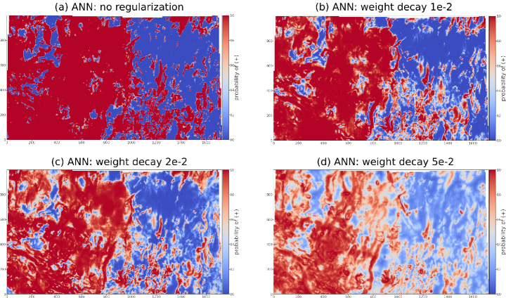
Figure 4: ANN model: illustration of reducing overfitting and overconfidence with regularization. Plotted are maps of the probability $p=P(\mathbf{x},{\bm{\gamma}})$ predicted by the neural network. (a) Shows the optimized model without regularization. (b-c) show the effect of stronger regularization as controlled by increasing the weight decay parameter. For reference, these maps and those that follow overlay the gray area of Figure 1, where north/south is aligned approximately up/down on the page and the axis units represent the indexes of the $250\textrm{m}\times 250\textrm{m}$ square pixels. See text for further discussion.

3.5.2 Discussion of variability in predictions

Suppose that we have a way to choose the “best” regularization method such that all model parameters are fixed. We find now that we have a remaining variability in the predictions of the network when it is trained multiple times. Training of artificial neural networks begins with a starting set of weights and biases, usually set at random, and the optimizer modifies these throughout the training stage toward a set of optimum values.

For complex problems it is often the case that there is a highly nonlinear relationship among the features and the outcome, the features may not comprise a complete description of the physical process, and the features may be further contaminated by measurement noise. In this case there may not be an easily discoverable global minimum in the cost function for the problem, but many local minima may exist. Thus any training episode, given its random initial configuration may not end up in the same place. This is not easy to see by simply watching the learning curves and by evaluating the various performance metrics. It does become apparent for this problem when predictions are made to produce geothermal resource maps in unknown regions of the study area. Figure 5 illustrates this problem well.

In this example, the regularizing parameters of Figure 4d were set and 10 optimizations were performed, each producing a resource map. Variability among trials arises from random seeding of the weights and biases within the network. Figure 5a and 5b show two such maps with example regions highlighted with circles. One can see noticeable differences in the map details within these regions, yet it is not obvious everywhere that they are different. Figure 5c shows the average of 10 such maps, and Figure 5d shows the standard deviation among these maps. It seems that some geographic areas are simply more prone to variability than others, leading us to the conclusion that the uncertainty varies significantly spatially. This needs to be reconciled for confident application of the results.

In what follows we describe a modification of the neural network model that incorporates both of these forms of uncertainty and provides useful quantitative measures of confidence and variability.

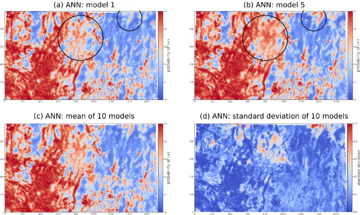
Figure 5: ANN model variability exposed by multiple runs, each having a different random number seed. Plotted are maps of the probability $p=P(\mathbf{x},{\bm{\gamma}})$ predicted by the neural network. ANN models #1 (a) and #5 (b) represent the extreme variability seen among 10 training trials. A comparison of the two extremes to the mean (c) and the standard deviation (d) of all 10 trials shows that there is significant variability due to random effects from one training trial to another. Note extreme examples within the circular regions.

4 Variational Inference with Bayesian Neural Networks

4.1 Paradigm

As we have seen, the direct application of artificial neural networks to the problem of geothermal resource assessment warrants further analysis of model uncertainty. First, we wish to quantify the variability in the state of the “best” model resulting from seemingly identical successive training efforts. Second, once a model is chosen we wish to define useful confidence bounds for predictions arising during prediction. Together these issues expose aspects of aleatoric and/or epistemic uncertainty. Hüllermeier and Waegeman, (2021) provide a lucid description of these concepts in the context of machine learning models. We summarize some of their key points here.

Machine learning involves the extraction of reasonable models from data by example. The goal is to generalize from the cases presented to the algorithm during training to new and yet unseen examples from the data generating (physical) process. The resulting models can never be proven to be correct, but remain hypothetical and uncertain.

Aleatoric, or statistical, uncertainty refers to the variability in the outcome due to random effects. In this application the following sources of randomness are related to feature input data: inherent randomness in geophysical and geoglogic features, measurement error, and interpolation or smoothing between geographic measurement points. There are also model related sources of variability, including: random initialization of weights, dropout regularization, incomplete convergence due to early termination of training, and convergence to a one of perhaps many local minima in a complex cost function. These sources of uncertainty are considered “irreducible” in that they cannot in practice be reduced to an arbitrary desired level.

Epistemic uncertainty represents the lack of knowledge about the best model to use by the decision maker and not to any underlying random process. This type of uncertainty can be reduced in principle through incorporating additional information. Such information could include the addition of further training examples, augmentation of the feature set through engineering the features themselves or adding new data types, or adding to or modifying the set of model hypotheses considered in the search for the best model (such as modifying the neural network architecture). These sources of uncertainty are under our control and so epistemic uncertainty refers to the “reducible” part of the total.

Since we use artificial neural networks, epistemic uncertainty is assumed to be uncertainty about the model parameters ${\bm{\gamma}}$, that is, the values of both the weights and biases ${\bm{\gamma}}=(\mathbf{W},\mathbf{b})$. Bayesian neural networks (Denker and LeCun,, 1991) represent a paradigm that captures this type of uncertainty. We note, however, that the Bayseian neural network approach does not explicitly recognize the dichotomy among nor attempt to isolate different sources of uncertainty.

Using the Bayesian approach, instead of having a fixed set of single-valued model parameters to be optimized, each weight and bias in the network is represented by its own probability distribution. Learning the parameters of these distributions comes about in essence by the application of Bayes’s rule (e.g. Bishop,, 2006). Thus the posterior of the weight distributions is computed as an update from our prior assumptions or knowledge by considering the evidence from the training data.

The motivation for the use of Bayesian neural networks is that they allow us to both naturally incorporate model variability and to provide confidence bounds for our predictions. This approach includes the epistemic uncertainty described above and also incorporates the model related sources of variability listed in the aleatoric category. We leave analysis of the data-related uncertainty in the machine learning models for another time.

In the following sections, we develop this concept from theory to practice. Beginning with a discussion of the classification problem, we summarize the formalism for the use of Bayesian neural networks (BNN) and in so doing we underscore the meaning of the outputs of these models. Finally, we provide notes on their implementation and optimization and finish with the application to geothermal resource assessment.

4.2 Mathematical Formulation for BNN

4.2.1 Bayesian Neural Network

Reiterating from Section 3.2, the function $P$ in Equation (4) represents a deterministic neural network that predicts the proportion of positive sites among a population of sites characterized by a feature vector $\mathbf{x}$. The second argument of $P$, the vector ${\bm{\gamma}}$, represents the network parameters (weights and biases). A Bayesian neural network, in contrast, predicts a probability density function (PDF) of $p$ based on a specified PDF of ${\bm{\gamma}}$, again for given $\mathbf{x}$. Denoting the PDF of ${\bm{\gamma}}$ as $f({\bm{\gamma}})$, a Bayesian network evaluates

$$f(p\kern 0.74997pt|\kern 0.74997pt\mathbf{x}) =\int|\mathrm{d}{\bm{\gamma}}|\ f(p\kern 0.74997pt|\kern 0.74997pt\mathbf{x},{\bm{\gamma}})\kern 0.74997ptf({\bm{\gamma}})$$ (14)

where $|\mathrm{d}{\bm{\gamma}}|=\mathrm{d}\gamma_{1}\kern 0.74997pt\mathrm{d}\gamma_{2}\kern 0.74997pt\cdots$ denotes the differential volume in ${\bm{\gamma}}$-space and where the integration is over the entire space. This equation follows from the definitions of marginal and conditional probability distributions and the requirement that the PDF of ${\bm{\gamma}}$ not depend on $\mathbf{x}$, i.e., $f({\bm{\gamma}}\kern 0.74997pt|\kern 0.74997pt\mathbf{x})=f({\bm{\gamma}})$. The deterministic function $P$ underlies this calculation in that (4) implies

$$f(p\kern 0.74997pt|\kern 0.74997pt\mathbf{x},{\bm{\gamma}}) =\delta(p-P(\mathbf{x},{\bm{\gamma}}))$$ (15)

$\delta$ being the Dirac delta function.

We note that, even for simple choices of $f({\bm{\gamma}})$, (14) cannot in general be reduced to an analytic expression given that $P$ is a nonlinear function of ${\bm{\gamma}}$. Therefore, our implementation of Bayesian networks represents $f(p\kern 0.74997pt|\kern 0.74997pt\mathbf{x})$ indirectly as a set of random samples drawn from this PDF: $p_{k}$, $k=1$, 2, …. These are generated as $p_{k}=P(\mathbf{x},{\bm{\gamma}}_{k})$ where each ${\bm{\gamma}}_{k}$ is a random samples from $f({\bm{\gamma}})$. The samples $p_{k}$ can be used to construct a histogram that serves as an approximation to $f(p\kern 0.74997pt|\kern 0.74997pt\mathbf{x})$, and to estimate moments or quantiles of $f(p\kern 0.74997pt|\kern 0.74997pt\mathbf{x})$.

Given $f(p\kern 0.74997pt|\kern 0.74997pt\mathbf{x})$, one can derive the PMF of the discrete random variable $y$ as follows. First we express the PMF as (similar to (14))

$$f(y\kern 0.74997pt|\kern 0.74997pt\mathbf{x}) =\int_{0}^{1}\mathrm{d}p\ f(y\kern 0.74997pt|\kern 0.74997ptp,\mathbf{x})\kern 0.74997ptf(p\kern 0.74997pt|\kern 0.74997pt\mathbf{x}).$$ (16)

Substituting the Bernoulli model of Equations (1) and (3) we have

$$f(y\kern 0.74997pt|\kern 0.74997pt\mathbf{x}) =\int_{0}^{1}\mathrm{d}p\ p^{y}\kern 0.74997pt(1-p)^{1-y}\kern 0.74997ptf(p\kern 0.74997pt|\kern 0.74997pt\mathbf{x}).$$ (17)

Evaluating this integral separately for $y=0$ and 1, then recombining, we obtain

$$f(y\kern 0.74997pt|\kern 0.74997pt\mathbf{x}) ={\bar{P}}(\mathbf{x})^{y}\kern 0.74997pt\big{(}1-{\bar{P}}(\mathbf{x})\big{)}^{1-y}$$ (18)

where

$${\bar{P}}(\mathbf{x}) =\int_{0}^{1}\mathrm{d}p\ p\kern 0.74997ptf(p\kern 0.74997pt|\kern 0.74997pt\mathbf{x}).$$ (19)

We see that $y$ still follows a Bernoulli distribution, with the probability of success given by the mean of $f(p\kern 0.74997pt|\kern 0.74997pt\mathbf{x})$.

4.2.2 Training the Bayesian Network

With a Bayesian neural network the training data are used to learn the PDF $f({\bm{\gamma}})$, as opposed to learning a single, best-fitting value of ${\bm{\gamma}}$. True to its name, a Bayesian network enlists Bayesian inference for this task. That is, $f({\bm{\gamma}})$ is taken to be the posterior PDF of ${\bm{\gamma}}$, which we denote $f_{\mathsf{pos}}({\bm{\gamma}})$, as informed by the training data. Applying Bayes’s rule we have

$$f_{\mathsf{pos}}({\bm{\gamma}}) \equiv f({\bm{\gamma}}\kern 0.74997pt|\kern 0.74997ptX,Y)=\frac{f(Y\kern 0.74997pt|\kern 0.74997ptX,{\bm{\gamma}})\kern 0.74997ptf_{\mathsf{pri}}({\bm{\gamma}})}{f(Y\kern 0.74997pt|\kern 0.74997ptX)}$$ (20)

where $f_{\mathsf{pri}}({\bm{\gamma}})$ is an assigned prior PDF of ${\bm{\gamma}}$, $f(Y\kern 0.74997pt|\kern 0.74997ptX,{\bm{\gamma}})$ is the likelihood function given by Equation (11), and

$$f(Y\kern 0.74997pt|\kern 0.74997ptX) =\int|\mathrm{d}{\bm{\gamma}}|\ f(Y\kern 0.74997pt|\kern 0.74997ptX,{\bm{\gamma}})\kern 0.74997ptf_{\mathsf{pri}}({\bm{\gamma}})$$ (21)

which is the PDF of $Y$ marginalized with respect to ${\bm{\gamma}}$.

As we noted in Section 4.2.1, the direct computation of $f(p\kern 0.74997pt|\kern 0.74997pt\mathbf{x})$ is in general not feasible and certainly not when the PDF of ${\bm{\gamma}}$ is taken to be the Bayesian posterior, $f_{\mathsf{pos}}$ in (20). The alternative of generating random samples from $f(p\kern 0.74997pt|\kern 0.74997pt\mathbf{x})$ also faces computational challenges in requiring the sampling of $f_{\mathsf{pos}}({\bm{\gamma}})$. To accommodate this requirement, we adopted the variational Bayes method to obtain an approximation to $f_{\mathsf{pos}}$ amenable to efficient sampling.

4.2.3 Variational Bayes

In the variational Bayes method $f_{\mathsf{pos}}({\bm{\gamma}})$ is approximated with a convenient representation involving a vector of parameters, ${\bm{\theta}}$: $f_{\mathsf{pos}}({\bm{\gamma}})\approx g({\bm{\gamma}};{\bm{\theta}})$. In this study we took $g$ to be a multivariate Gaussian p.d.f. with the components of ${\bm{\theta}}$ comprising the means and variances of the components of ${\bm{\gamma}}$ (the neural network biases and weights). The covariances between network parameters were assumed to be zero, reducing the sampling of $g({\bm{\gamma}};{\bm{\theta}})$ to the easy task of sampling univariate Gaussian distributions.

Variational Bayes seeks the value of ${\bm{\theta}}$ that minimizes the discrepancy between $g$ and $f_{\mathsf{pos}}$, as quantified by the Kullback-Leibler (KL) divergence of $g$ from $f_{\mathsf{pos}}$. Goodfellow et al., (2016, Chapter 3) provide further context for use of the KL divergence in terms of Information Theory. In our notation it is defined as:

$$D_{\mathsf{KL}}[g||f_{\mathsf{pos}}] =\int|\mathrm{d}{\bm{\gamma}}|\ g({\bm{\gamma}};{\bm{\theta}})\kern 0.74997pt\log\left(\frac{g({\bm{\gamma}};{\bm{\theta}})}{f_{\mathsf{pos}}({\bm{\gamma}})}\right)$$ (22)

where the integration is performed over the support of $g$, i.e. the regions of ${\bm{\gamma}}$-space in which $g>0$. We recognize this as an expected value with respect to ${\bm{\gamma}}$, using $g$ as its PDF. For any function of ${\bm{\gamma}}$, $\phi({\bm{\gamma}})$, let us define

$$\mathop{\mathbb{missing}}{E}\nolimits_{g}\big{[}\phi({\bm{\gamma}})\big{]} =\int|\mathrm{d}{\bm{\gamma}}|\ g({\bm{\gamma}};{\bm{\theta}})\kern 0.74997pt\phi({\bm{\gamma}}).$$ (23)

We can then write (22) as

$$D_{\mathsf{KL}}[g||f_{\mathsf{pos}}] =\mathop{\mathbb{missing}}{E}\nolimits_{g}\left[\log\left(\frac{g({\bm{\gamma}};{\bm{\theta}})}{f_{\mathsf{pos}}({\bm{\gamma}})}\right)\right].$$ (24)

Plugging in Equation (20) (Bayes’s rule) and expanding the logarithm, we get

$$D_{\mathsf{KL}}[g||f_{\mathsf{pos}}] =\mathop{\mathbb{missing}}{E}\nolimits_{g}\left[\log\left(\frac{g({\bm{\gamma}};{\bm{\theta}})\kern 0.74997ptf(Y\kern 0.74997pt|\kern 0.74997ptX)}{f(Y\kern 0.74997pt|\kern 0.74997ptX,{\bm{\gamma}})\kern 0.74997ptf_{\mathsf{pri}}({\bm{\gamma}})}\right)\right]$$

$$=-\mathop{\mathbb{missing}}{E}\nolimits_{g}\Big{[}\log f(Y\kern 0.74997pt|\kern 0.74997ptX,{\bm{\gamma}})\Big{]}+\mathop{\mathbb{missing}}{E}\nolimits_{g}\left[\log\left(\frac{g({\bm{\gamma}};{\bm{\theta}})}{f_{\mathsf{pri}}({\bm{\gamma}})}\right)\right]+\log f(Y\kern 0.74997pt|\kern 0.74997ptX).$$ (25)

We recognize the first term on the right-hand side of (25) as the expected value of the negative log-likelihood function, ${\cal L}$ in Equation (12), and the second term as the KL divergence of $g$ from the prior distribution $f_{\mathsf{pri}}$. Since the third term does not depend on ${\bm{\theta}}$, we can thus express the variational Bayes solution for ${\bm{\theta}}$ as

$${\bm{\theta}}_{\mathsf{VB}} =\arg\min_{\bm{\theta}}{\cal K}({\bm{\theta}};X,Y)$$ (26)

where the objective, or cost, function ${\cal K}$ is given by

$${\cal K}({\bm{\theta}};X,Y) =\mathop{\mathbb{missing}}{E}\nolimits_{g}{\cal L}({\bm{\gamma}};X,Y)+D_{\mathsf{KL}}[g||f_{\mathsf{pri}}].$$ (27)

We observe that the first term of ${\cal K}$ is the expected value of the cost function minimized in deterministic network training (to obtain ${\bm{\gamma}}_{\mathsf{ML}}$), while the second term serves as a penalty function that regularizes ${\bm{\theta}}_{\mathsf{VB}}$.

We use a gradient descent method to minimize the cost function ${\cal K}$. The algorithm is similar to that used to calculate ${\bm{\gamma}}_{\mathsf{ML}}$ for a deterministic neural network but with some notable differences. In particular, since ${\cal K}$ includes a penalty term, we do not invoke regularization procedures (like dropout) within the gradient descent loop. Further, evaluation of the cost function and its gradient now entails finding an expected value with respect to ${\bm{\gamma}}$, by virtue of the first term of (27). This is accomplished by averaging ${\cal L}$ and its gradient over values of ${\bm{\gamma}}$ randomly sampled from $g({\bm{\gamma}};{\bm{\theta}})$, with ${\bm{\theta}}$ fixed to its current value at each step of the descent. Further details of our computational approach are given below in Section 4.3.

4.2.4 Regularization Parameter

Within the Bayesian inference paradigm, the cost function ${\cal K}$ in (27) optimally pools the information provided by the training data and by prior knowledge. However, this optimality assumes that the statistical models for the two sources of information are equally credible and well calibrated, which is not the case in the application presented here. In particular, the prior distribution assigned to neural network parameters, $f_{\mathsf{pri}}({\bm{\gamma}})$, is at best conjectural. The formal remedy for such deficiencies is to introduce unknown hyperparameters into the statistical models for the training data and prior information. The selection of these parameters is addressed within the Bayesian inference paradigm with the goal of balancing the two sources of information to avoid overfitting or underfitting the training data.

In this project we applied a simple version of this remedy by introducing a single hyperparameter, $\alpha>0$, and replacing the cost function in Equation (27) with

$${\cal K}({\bm{\theta}};X,Y) =\mathop{\mathbb{missing}}{E}\nolimits_{g}{\cal L}({\bm{\gamma}};X,Y)+\alpha\kern 0.74997ptD_{\mathsf{KL}}[g||f_{\mathsf{pri}}].$$ (28)

By scaling the penalty term, $\alpha$ plays the role of a regularization parameter as used in inversion methods like Tikhonov regularization. We note that in some problems a regularization parameter can be identified with a parameter of the underlying statistical model, such as the variance of a measurement error or a prior variance of the unknown parameters. In our variational Bayes application, with the Bernoulli model assumed for training data, $\alpha$ does not have such a simple interpretation. In Section 4.4 we suggest that $\alpha$ controls the model complexity and following this notion we propose a practical numerical procedure for selecting it.

4.2.5 Interpretation of $f(p\kern 0.74997pt|\kern 0.74997pt\mathbf{x})$

Our classification framework bases the assessment of a prospective geothermal site with feature vector $\mathbf{x}$ on the PDF $f(p\kern 0.74997pt|\kern 0.74997pt\mathbf{x})$, as calculated by the Bayesian neural network trained with data from known positive and negative sites. The parameter $p$ is the proportion of positive sites among all sites sharing feature vector $\mathbf{x}$. Its PDF quantifies our uncertainty about its true value and can be used, for example, to construct confidence intervals (or credibility intervals) on $p$, or to test hypotheses about $p$.

The goal of the classification problem, however, is to predict the class of a site, $y$, based on its PMF, $f(y\kern 0.74997pt|\kern 0.74997pt\mathbf{x})$. Owing to the simplicity of the Bernoulli model, our analysis concluded that $f(y\kern 0.74997pt|\kern 0.74997pt\mathbf{x})$ depended only on the mean of $f(p\kern 0.74997pt|\kern 0.74997pt\mathbf{x})$ and not its shape. Effectively, uncertainty in the value of $p$ does not affect uncertainty in $y$. Yet, intuitively, the shape of $f(p\kern 0.74997pt|\kern 0.74997pt\mathbf{x})$ should play a role in deciding how to classify a site. In particular, it would be reasonable to consider the dispersion of $f(p\kern 0.74997pt|\kern 0.74997pt\mathbf{x})$ about the mean — the width of the distribution — in deciding whether or not a site is positive. For a given mean, a smaller dispersion should make one feel more confident in the class assigned to a site.

While this seeming deficiency in our analysis might be remedied with a more sophisticated statistical model, it partly stems from the fundamental meaning of probability. A probability predicts the average outcome of a repeated random experiment over the long run. In our problem, an experiment can be viewed as a two-step process: first select $p$ at random from $f(p\kern 0.74997pt|\kern 0.74997pt\mathbf{x})$, and then draw a site at random from the population of sites that have a proportion $p$ of positive sites. Our analysis showed that, over the long run, the proportion of outcomes with $y=1$ (positive sites) will be ${\bar{p}}$, the mean of $f(p\kern 0.74997pt|\kern 0.74997pt\mathbf{x})$. Outcomes where the first step yields $p<{\bar{p}}$ will negate those yielding $p>{\bar{p}}$, regardless of the shape of $f(p\kern 0.74997pt|\kern 0.74997pt\mathbf{x})$.

However, a decision maker concerned about false positives (classifying negative sites as positive) might want to perform a “worst case,” rather than average case, analysis and consider the following two-step experiment: randomly select $K$ (say, ten) values of $p$ from $f(p\kern 0.74997pt|\kern 0.74997pt\mathbf{x})$ and then draw a site at random from the population having the smallest $p$ among the $K$ samples. Pursuing this idea, let $F(p\kern 0.74997pt|\kern 0.74997pt\mathbf{x})$ be the cumulative distribution function (CDF) associated with $f(p\kern 0.74997pt|\kern 0.74997pt\mathbf{x})$:

$$F(p\kern 0.74997pt|\kern 0.74997pt\mathbf{x}) =\int_{0}^{p}\mathrm{d}p^{\prime}\ f(p^{\prime}\kern 0.74997pt|\kern 0.74997pt\mathbf{x}).$$ (29)

Using integration by parts, one can verify that

$${\bar{p}} \equiv\int_{0}^{1}\mathrm{d}p\ p\kern 0.74997ptf(p\kern 0.74997pt|\kern 0.74997pt\mathbf{x})=\int_{0}^{1}\mathrm{d}p\ \big{(}1-F(p\kern 0.74997pt|\kern 0.74997pt\mathbf{x})\big{)}.$$ (30)

Now denote the PDF and CDF of the worst-of-$K$ version of $p$ as $f_{\mathsf{worst}}$ and $F_{\mathsf{worst}}$, respectively. A basic result of order statistics (e.g. David,, 1981) is

$$1-F_{\mathsf{worst}}(p\kern 0.74997pt|\kern 0.74997pt\mathbf{x}) =\big{(}1-F(p\kern 0.74997pt|\kern 0.74997pt\mathbf{x})\big{)}^{K}.$$ (31)

It follows that the mean of $f_{\mathsf{worst}}(p\kern 0.74997pt|\kern 0.74997pt\mathbf{x})$, which becomes the inferred probability of a positive site in this worst-of-$K$ analysis, is

$${\bar{p}}_{\mathsf{worst}} =\int_{0}^{1}\mathrm{d}p\ \big{(}1-F(p\kern 0.74997pt|\kern 0.74997pt\mathbf{x})\big{)}^{K}.$$ (32)

It happens that ${\bar{p}}_{\mathsf{worst}}$ is less than ${\bar{p}}$ and does depend on the shape of $f(p\kern 0.74997pt|\kern 0.74997pt\mathbf{x})$, with ${\bar{p}}_{\mathsf{worst}}$ deceasing as the dispersion of $f(p\kern 0.74997pt|\kern 0.74997pt\mathbf{x})$ increases.

To acknowledge the role uncertainty in $p$ plays in site classification, without committing to a particular decision strategy, the results of the next section display a quantile of $f(p\kern 0.74997pt|\kern 0.74997pt\mathbf{x})$ rather then its mean. Namely, we show the value of $p$ satisfying

$$F(p\kern 0.74997pt|\kern 0.74997pt\mathbf{x}) =\beta$$ (33)

for some choice of $\beta$. A neutral choice would be $\beta=0.5$ but we have chosen $\beta=.05$ to reflect a greater aversion to false positive classifications than false negative classifications.

4.3 Implementation

The implementation of a Bayesian neural network involves several key changes to that of the deterministic fully connected network described earlier in Algorithms 1 and 2. Before, the network model was determined by a single set of deterministic parameters (weights and biases). In the Bayesian case the network is determined by distributions of weights and biases, in effect representing an infinite family of models. For practical purposes each parameter distribution is assumed to be Gaussian, parameterized by its mean and standard deviation. Thus, the number of parameters defining a Bayesian neural network is twice that of a deterministic neural network with the same architecture.

When the model is used for prediction, a specific set of weights and biases must first be sampled from the distributions for each node in the network. The key elements of sampling from the posterior distributions of the weights and biases are described in Algorithm 3. Then, once this posterior sampling is performed, a fixed set of weights and biases is in hand and can then be used to generate a prediction using the same algorithm as in the standard network (Algorithm 1).

Algorithm 3 Sampling from the posterior distributions of weights and biases for a Bayesian neural network. The network is defined probabilistically with normal distributions of weights and biases. Each of these distributions is parameterized by its mean $\mu$ and standard deviation $\sigma$. To facilitate training, the standard deviation is forced to be positive by using an intermediate real-valued parameter $\rho$ and then applying the PyTorch softplus function (e.g. Paszke et al.,, 2019). Forward passes through the network first require sampling from these posterior distributions. 1:procedure SamplePosteriors($\bm{\rho},\bm{\mu}$) 2:     for all weight elements i do $\triangleright$ weight matrices 3:         $\sigma^{[w]}_{i}\leftarrow\log(1+\exp(\rho^{[w]}_{i}))$ $\triangleright$ create a positive standard deviation with softplus 4:         $w_{i}\leftarrow\mathcal{N}(0,1)\cdot\sigma^{[w]}_{i}+\mu^{[w]}_{i}$ $\triangleright$ sample from a standard normal distribution and scale       5:     for all bias elements j do $\triangleright$ bias vectors 6:         $\sigma^{[b]}_{j}\leftarrow\log(1+\exp(\rho^{[b]}_{j}))$ $\triangleright$ create a positive standard deviation with softplus 7:         $b_{j}\leftarrow\mathcal{N}(0,1)\cdot\sigma^{[b]}_{j}+\mu^{[b]}_{j}$ $\triangleright$ sample from a standard normal distribution and scale       8:     return $\mathbf{W}$, $\mathbf{b}$ $\triangleright$ return weights and biases

The training of a Bayesian neural network contains some further modifications from the deterministic case as described in Algorithm 4. First, the cost function being optimized (minimized) is now ${\cal K}$ in Equation (28). For each training iteration the algorithm employs a sampling of the posteriors before predictions are made. This is an important nuance, since the likelihood term is now an expected value (i.e. $\mathop{\mathbb{missing}}{E}\nolimits_{g}$) with respect to the posterior of ${\bm{\gamma}}$. Since each posterior sampling and forward pass is merely a sample from the model set then we must gather some statistics of the properties of the model in order to meaningfully update the mean and standard deviation of each weight and bias distribution. Therefore, several realizations of the model are probed and accumulated – first using posterior sampling, then a forward pass, and then computation of the cost – before updating the statistics (means and standard deviations) of the weight and bias distributions. Finally, we note that in training a Bayesian network the cost function is now composed of two terms, one a penalty for model complexity and the other a penalty for misfit to the training data (Equation (28)). The balance between these two terms is determined by an important heuristic parameter, $\alpha$. A suitable choice of this heuristic is described in the next section.

Algorithm 4 Training a Bayesian neural network (see text for explanation). 1:choice of prior distributions for weights and biases 2:choice of cost function heuristic parameter, $\alpha$ 3:choice of model hyperparameters 4:randomly initialized posterior parameters for weights and biases, $\rho$ and $\mu$ 5:choice of number of samples for gathering posterior statistics, $N_{samples}$ 6:procedure Train($\bm{X},\bm{Y}$) $\triangleright$ input all training example features and labels 7:     repeat 8:         $\mathcal{L}\leftarrow 0$ $\triangleright$ set cost to 0 9:         for all $\mathbf{x},y$ in $\bm{X}$, $\bm{Y}$ do $\triangleright$ consider each training example 10:              for $j$ in $N_{samples}$ do $\triangleright$ gather statistics of posteriors 11:                  $\mathbf{W}_{j},\mathbf{b}_{j}\leftarrow\textrm{SamplePosteriors}(\bm{\rho},\bm{\mu})$ $\triangleright$ sample the posterior distributions 12:                  $\hat{y}_{j}\leftarrow\textrm{ForwardPass}(\mathbf{x},\mathbf{W}_{j},\mathbf{b}_{j})$ $\triangleright$ predict with a forward pass through the network 13:                  $\mathcal{L}_{j}\leftarrow\textrm{Cost}(y,\hat{y}_{j},\textrm{priors},\bm{\rho},\bm{\mu},\alpha)$ $\triangleright$ cost balancing data misfit and model complexity                14:              $\mathcal{L}_{N}\leftarrow\sum\mathcal{L}_{j}/N_{samples}$ $\triangleright$ Average cost for $N_{samples}$ 15:              $\mathcal{L}\leftarrow\mathcal{L}+\mathcal{L}_{N}$ $\triangleright$ sum the cost of misfit to all data           16:         $\bm{\rho},\bm{\mu}\leftarrow\textrm{Update}(\textrm{Optimizer},\mathcal{L})$ $\triangleright$ update model based on total cost 17:     until model is optimized 18:     return $\bm{\rho},\bm{\mu}$ $\triangleright$ return optimized model parameters

4.4 Modeling

We now have in hand a formulation of a Bayesian neural network clarifying the interpretation of the outcomes and an algorithm for its implementation on a computer. We next explore the properties of this approach and compare them to the deterministic neural network discussed earlier.

4.4.1 Controlling the Model Complexity

In this discussion we refer to the cost function of Equation (28) which controls the balance between model complexity and data fit by varying a regularization parameter $\alpha$. We illustrate the effect of $\alpha$ by example in Figure 6.

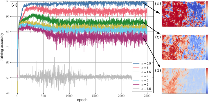
Figure 6: Illustration of the control of model complexity by varying the regularization parameter $\alpha$. (a) shows a sequence of learning curves tracking the evolution of the training accuracy with training epoch. As $\alpha$ increases the final training accuracy at epoch 2500 decreases systematically and moves from overfitting (where accuracy approaches 100% at $\alpha=0.5$) to not being able to classify any longer (where accuracy is about 50% at $\alpha=5.5$). The effect of varying $\alpha$ in this range is shown in (b-d) where more reasonable maps result at intermediate values of regularization.

The same feature data set and geothermal site labels used in the previous examples were used to optimize a set of Bayesian models by varying the regularization parameter $\alpha$. To illustrate this process, we monitor the training accuracy learning curves along with examples of the resulting predicted geothermal potential maps (see in Figure 6). Focusing on the learning curves, we see that for small values of $\alpha$, where the data fit term in the loss dominates, the model attains high accuracy. This is also true for testing accuracy, but this is not shown here. As the regularization parameter is increased, the training accuracy goes down until at some point the algorithm fails to classify the examples and the training accuracy abruptly drops to about 50%.

We also show the maps of the study area produced by several examples of the trained models. For the small $\alpha$ and high training accuracy cases the geothermal resource maps are effectively binary in character … the model largely predicts either a positive geothermal resource or a negative one with little in between. There is no nuance in the predictions and an unrealistically large proportion of the study area are predicted to be positive sites. These models are therefore not useful.

When $\alpha$ increases, however, the maps have nuance in the predictions, there is a much lower overall areal proportion of high resource potential, and the maps more closely resemble the results from the original PFA study. This all serves to illustrate the importance of properly choosing the regularizing parameter in order to obtain a useful and defensible result.

4.4.2 An Optimal Degree of Regularization

We conclude that the key to finding an optimal degree of regularization is to consider the information content a particular model is capable of holding. After a brief review of some literature on this subject we will pose a first order and workable choice of the regularization parameter based on this concept.

Background.

We have seen the need to regularize the solution by varying the parameter $\alpha$ in Equation (28) that balances the fit to the data and the complexity of the model. It is tempting to treat this regularization process, not as a simple heuristic choice, but instead tie it to a quantifiable measure defining a best solution.

Some inspiration can be derived from the literature describing inversion via the maximum entropy principle. The works by Gull, Skilling, and others (Gull and Daniell,, 1978; Gull,, 1989; Skilling,, 1989, 1990; Skilling and Gull,, 1991) provide good descriptions of this concept and its application. In these papers a solution is sought that contains no more structure than the experimental data “allow.” For example, in an image processing problem, Gull, (1989) considers a heuristic similar to ours and identifies it with the model complexity and further links it to the (hopefully) countable number of “good” or accurate singular vectors contained in the data.

The concept of degrees of freedom is discussed lucidly by Walker, (1940), where it is described as the number of free parameters available to adjust a geometric figure in an N-dimensional space. Of significance to our problem is the consideration of a hyperplane, defined as any equation of the first degree connecting the N variables. For example, a line in two-dimensional space is a hyperplane, as is a plane in three-dimensional space, etc. A hyperplane has N-1 degrees of freedom of movement on it and, in its simplest form, N parameters to define it. The simplest decision boundary one could seek in an N-dimensional classification problem would be a hyperplane.

Abu-Mostafa et al., (2012) summarize the definition and significance of the Vapnik–Chervonenkis (or VC) dimension, $d_{VC}$, as measure of model complexity. This gives both an upper bound to the “out-of-sample” error and the “effective” number of degrees of freedom of the model under consideration. This concept is said to provide a means for choosing the best regularizing parameter, and using the VC dimension in this way has the same goal as cross-validation, the process of choosing a regularization parameter by ensuring optimal generalization by using a hold-out data set (e.g. Goodfellow et al.,, 2016). This concept holds for any model, be it a neural network, support vector machine (e.g. Goodfellow et al.,, 2016, Chapter 5), or other. An interesting end member case is that of the perceptron, where the VC dimension is equal to one more than the number of features, i.e. $d_{VC}=N+1$, a value close to the number of parameters needed to specify a hyperplane.

Yet other attempts to balance the data fit and model complexity make use of the Akaike Information Criterion (AIC) and the Bayesian Information Criterion (BIC) and their variants (e.g. Fabozzi et al.,, 2014). Such concepts of defining model complexity and information content just mentioned and more have been discussed widely in the literature in the search for the perfect heuristic for choice of regularization. In consideration of artificial neural networks some notable further examples are espoused by Hinton and van Camp, (1993), Fisher, (2003), Kline and Bourgeois, (2010), Gao and Jojic, (2016), and Maddox et al., (2020).

In principle, then, we are presented with the problem of finding a model that is as simple as possible, that fits our training data, and generalizes well to test data during cross validation and thereby honoring the information available in the data set in the presence of noise, measurement error, etc. Ideally, we also have some useful metrics to aid us in this search. In practical problems the key question is whether or not we can measure or estimate all of the quantities required by the theories.

Guided by these concepts, and in light of our unaccounted-for possible measurement errors and noise, in the following few sections we describe our approach to find a conservative degree of regularization.

Counting Degrees of Freedom.

An artificial neural network contains a fixed number of free parameters (weights and biases) controlling the nonlinear combinations of input features. Among the large number of parameters a model contains, once the model is trained only a relatively small number contribute significantly to the final predictions. One can imagine determining the number of dominant model parameters by counting those larger than some threshold. This technique has been used frequently to “prune” a network to make it more compact in terms of memory use by setting weights smaller than a threshold to zero and perhaps reconfiguring the architecture (e.g. Han et al.,, 2015). Choosing such a threshold could be considered somewhat arbitrary.

For our purposes using Bayesian neural networks, the problem is more straight forward. In the Bayesian case, the weights and biases are not fixed values but are instead drawn form probability distributions. These distributions are approximated by Gaussians and are each parameterized by their means and standard deviations. The useful realization is that if a particular distribution is too broad and has a mean too close to zero, then random samples from the distribution could take on both positive and negative values. If this happens too frequently during prediction, then that particular weight cannot possibly contribute effectively to the outcome as sometimes it would add a contribution and another time it would subtract. We therefore propose the following method for counting the effective degrees of freedom of a Bayesian neural network.

We begin with a trained model, which has been optimized with a particular choice of the regularization parameter $\alpha$. For this trained model we inspect all of the weight distributions and sort them by the absolute value of their ratios of the mean to the standard deviation, $|\mu/\sigma|$. We count a weight as useful and contributing to the number of degrees of freedom if $|\mu/\sigma|\geq 1$. On the other hand if $|\mu/\sigma|<1$ the weight is assumed to not be effective in the computations since too many random samples drawn from it are of alternating sign. In general. such noncontributing weights will also necessarily have a small value upon sampling, else they would simply add noise to the predictions.

We now show how this criterion can be applied to find a conservative value of the regularization parameter.

Search for an Optimal Regularizer.

It is illustrative to track the characteristics of our network as we optimize it over a range of regularization parameters. In Figure 7 we show typical results for the data loss, the training and testing accuracies, the AIC and BIC metrics, and the estimated number of degrees of freedom. We typically see the juxtaposition of two extremes, a dominance of the KL divergence term for low $\alpha$ characterized by a rapid change with $\alpha$ transitioning through a relatively distinct “knee” to dominance by the fit to data term characterized by a slow change. The “knee” in the curves is distinct and indicates some balance between the extremes yet is variable from one metric to the next and to our minds has no obvious intrinsic significance. We note, however, that the number of degrees of freedom curve provides us with a way to choose a value of $\alpha$ both conservative and understandable. Recall that the simplest decision boundary in our 10-feature problem would be a hyperplane with 9 free parameters and that the VC dimension for a linear perceptron in this case would be $d_{VC}=11$. We choose as a compromise 10 “effective” degrees of freedom by our measure to give a conservative solution to the problem, erring on the side of underfitting the data. Figure 8 shows how such a determination can be made. In our case we use the convention of normalizing the KL divergence as the average per number of weights in the network and normalizing the data fit as the data loss per training example. With this convention the optimal value of regularization is found to be $\alpha_{10}=3.65$. We note that for a range of $\alpha$ around this number, none of the model behavior characteristics varies greatly, and in fact the resulting predictive resource maps for this range are all visually similar.

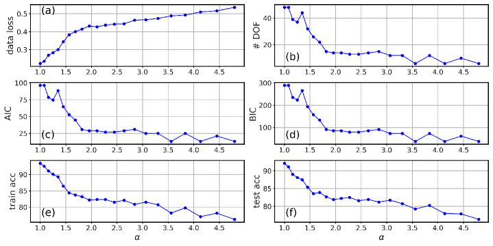
Figure 7: Metrics tracking effect of varying the regularization parameter $\alpha$. We show (a) the data loss, (b) our estimate of the number of degrees of freedom (DOF), (c) the Akaike Information Criterion (AIC), (d) the Bayes Information Criterion (BIC), (e) the training accuracy, and (f) the testing accuracy.

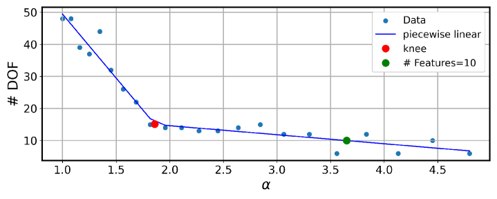
Figure 8: The data shown in Figure 7b, fit by a piece-wise (bilinear) function. The approximate position of the “knee” in the curve is shown with the red symbol and the position on the curve ($\alpha=3.65$) where the number of degrees of freedom equals the number of features (#DOF $=10$) is shown by the green symbol.

4.4.3 Variability in Predictions

Given we now have a favored degree of regularization, we can explore how well treating the problem as Bayesian has addressed one of the issues seen during the application of deterministic neural networks to this problem. Recall that the deterministic networks were found to hold a noticeable degree of variability from one trial to the next, which could not be easily understood or rectified. By including uncertainty into the problem with the Bayesian approach we had hoped to address this in a satisfactory way. Figure 9 shows the results. In the Bayesian neural network case, variability among trials arises from random seeding of the weights and biases distribution parameters $\mu$ and $\rho$ as well as the need to randomly draw multiple samples from the posteriors during prediction. In comparing this directly to the variability from the deterministic network trials (Figure 5), we see that now there is very small variability both in absolute value and spatially in the Bayesian neural network compared to the deterministic case. We consider, then, that the variability seen before has now been entrained into the way a Bayesian neural network can quantify the spread or distribution in outcomes of the model. This intrinsic variability now provides a measure of confidence in our predictions as we will discuss in a following section.

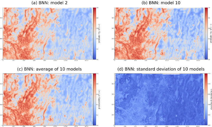
Figure 9: BNN model variability exposed by multiple runs. Each image represents an average of 128 samples from the posterior distribution of probabilities predicted by the neural network (which is an estimate of ${\bar{P}}(\mathbf{x})$, the mean of $f(p\kern 0.74997pt|\kern 0.74997pt\mathbf{x})$). BNN models #2 (a) and #10 (b) represent the extreme variability seen among 10 training trials. A comparison of the two extremes to the mean (c) and the standard deviation (d) of all 10 trials shows that there is very small variability both in absolute value and spatially in the Bayesian neural network compared to the deterministic case shown in Figure 5.

4.4.4 Synopsis

In summary, we have implemented a variational Bayesian approach for predicting geothermal energy resource potential in a stochastic way. The interpretation of the predictions at each site is shown to be a probability and conditioned on the evidence provided by the data. The predictions have been made intentionally in a conservative fashion. By optimizing the value of the regularization parameter we seek a model that is only as complex (and confident in its predictions) as the training data allow.

4.5 Results of the Favored Model

By using the Bayesian formulation for our problem, we have a final optimized model, which is probabilistic in nature. This provides a distinct advantage over a fixed-parameter neural network: that of providing a range of predictions for each case we wish to test whose spread represents a degree of reliability or confidence. Here we illustrate this outcome explicitly and suggest how it might be used to aid decision makers in the process of geothermal energy resource assessment or prospecting.

4.5.1 Distribution of Probabilities

Our trained and optimized model was used to make predictions of the probability of finding a viable geothermal resource (positive site) within each pixel (geographic area of 250m by 250m square) for the study area shown in Figure 1. Two maps help to illustrate the probabilistic nature of the result. Figure 10a shows the map for the mean of the distribution at each pixel and Figure 10b shows the standard deviation. These maps together give a sense of the geographic distribution of high and low geothermal resource probabilities as well as a measure of the corresponding spread or “uncertainty” in those values.

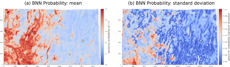
Figure 10: Geothermal resource potential model produced from a single training run at $\alpha_{10}=3.65$, the optimal value determined by consideration of model complexity described in Section 4.4.2. Predictions used to make the maps represent the average of 8192 samples from the posterior distribution of probabilities predicted by the neural network (which is an estimate of ${\bar{P}}(\mathbf{x})$, the mean of $f(p\kern 0.74997pt|\kern 0.74997pt\mathbf{x})$). (a) represents the mean posterior probability and (b) represents the standard deviation of posterior probability. The white triangle and circle symbols mark the locations of the example positive and negative training sites, respectively, shown in Figure 11.

These maps still do not tell the whole story. If one probes the resource probability distribution at specific pixels, one by one, then the true nature of this model are exposed. Figure 11 shows two typical distributions of the resource probability for specific example pixels taken from the training set: one positive site and one negative site. One can see the distributions can be highly skewed and may be multi-modal. Therefore, the simple mean and standard deviation maps are insufficient to describe the model properties in detail. It is clear that one should consider both the mean (which represents the average result if many drilling trials could be made) and the spread or range of this distribution to determine the variability that we expect to encounter. This has important practical applications, especially in cases where funding may allow only one chance to drill an exploratory hole.

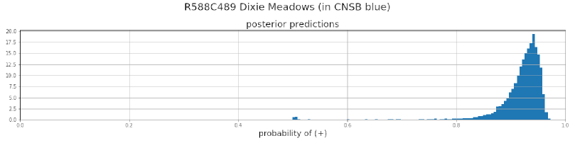
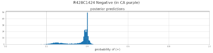
Figure 11: Examples of detailed posterior distributions $f(p\kern 0.74997pt|\kern 0.74997pt\mathbf{x})$ for two training sites. Top: The positive training site marked as a triangle in Figure 10. Bottom: The negative training site marked as a circle in Figure 10.

4.5.2 A Tool for Decision Makers

Given that probing the Earth for geothermal energy is expensive, often exceeding $2M for drilling a geothermal production or injection well (e.g. Lowry et al.,, 2017), we need to maximize our chances of success. A practical way of looking at the model in this regard is as follows. Looking at the individual distributions at specific pixels such as in Figure 11, we realize that our model actually represents a large family of models. If we construct the cumulative distribution function at each site, a specific quantile (or percentile) represents the number of the models that agree on a specific outcome. For example, the resource probability, say $p$, at the 0.5 quantile (50th percentile) represents where half of the models have a resource probability $>p$ and half have resource probability $<p$. More useful, for example, would be the 0.05 quantile or the 5th percentile. There, 95% of all models have resource probability $>p$ and only 5% smaller. A map constructed in this way (Figure 12) is much more conservative than the map of mean resource probabilities. High resource probability locations shown on this 0.05 quantile map carry much higher confidence and may be a practical tool for decision makers in the course of prospecting for new resources.

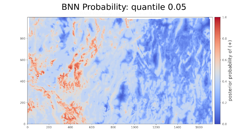
Figure 12: Posterior probability map for the $0.05$ quantile of $f(p\kern 0.74997pt|\kern 0.74997pt\mathbf{x})$ indicating where on the map 95% of the models have at least the probability shown by the color.

5 Summary

We have considered the application of machine learning to the evaluation of geothermal resource potential. A supervised learning problem was posed in terms of a set of maps based on 10 geological and geophysical features. These features were extracted from an extensive study in Nevada and were then used to classify geographic regions representing either a potential resource (+) or not (-). A training set of positive (known resources or active power plants) and negative training sites (known drill sites with unsuitable geothermal conditions) was used to constrain and optimize various artificial neural network models for this classification task. Among the models used, we found that by using a Bayesian approach we could naturally include model uncertainty and provide a way not only to predict resource potential but to also give measures of confidence or reliability.

Acknowledgements.

This work was supported in part by the U.S. Department of Energy’s Office of Energy Efficiency and Renewable Energy (EERE) under the Geothermal Technologies Program and Machine Learning Initiative award number DE-EE0008762.

References

- Abu-Mostafa et al., (2012) Abu-Mostafa, Y. S., M. Magdon-Ismail, and H.-T. Lin, 2012, Learning from data: AMLBook New York, NY, USA.
- Bishop, (2006) Bishop, C. M., 2006, Pattern recognition and machine learning (information science and statistics): Springer.
- Brown et al., (2020) Brown, S., M. Coolbaugh, J. DeAngelo, J. Faulds, M. Fehler, C. Gu, J. Queen, S. Treitel, C. Smith, and E. Mlawsky, 2020, Machine learning for natural resource assessment: an application to the blind geothermal systems of Nevada: Geothermal Resources Council Transactions, 44, 920–932.
- Coolbaugh et al., (2007) Coolbaugh, M., G. Raines, and R. Zehner, 2007, Assessment of exploration bias in data-driven predictive models and the estimation of undiscovered resources: Natural Resources Research, 16, 199–207.
- Craig et al., (2021) Craig, J., J. Faulds, N. Hinz, T. Earney, W. Schermerhorn, D. Siler, J. Glen, J. Peacock, M. Coolbaugh, and S. Deoreo, 2021, Discovery and analysis of a blind geothermal system in southeastern Gabbs Valley, western Nevada, USA: Geothermics, 97, 102177.
- Craig, (2018) Craig, J. W., 2018, Discovery and analysis of a blind geothermal system in southeastern Gabbs Valley, western Nevada: MS thesis, University of Nevada, Reno.
- David, (1981) David, H., 1981, Order statistics: Wiley. Wiley Series in Probability and Statistics.
- DeAngelo et al., (2021) DeAngelo, J., J. M. Glen, D. L. Siler, M. F. Coolbaugh, T. E. Earney, B. J. Dean, L. A. Zielinski, and B. T. Ritzinger, 2021, USGS contributions to the Nevada Geothermal Machine Learning Project (DE-FOA-0001956): Geophysics, heat flow, slip and dilation tendency: U.S. Geological Survey data release, https://doi.org/10.5066/P9V5SQRD.
- Denker and LeCun, (1991) Denker, J., and Y. LeCun, 1991, Transforming neural-net output levels to probability distributions: Presented at the Advances in Neural Information Processing Systems, Morgan-Kaufmann.
- Doust, (2010) Doust, H., 2010, The exploration play: What do we mean by it?: American Association of Petroleum Geologists Bulletin, 94, 1657–1672.
- Fabozzi et al., (2014) Fabozzi, F. J., S. M. Focardi, S. T. Rachev, and B. G. Arshanapalli, 2014, Appendix E: Model selection criterion: AIC and BIC, in The Basics of Financial Econometrics: Tools, Concepts, and Asset Management Applications: John Wiley & Sons, Ltd, 399–403.
- Faulds et al., (2020) Faulds, J., S. Brown, M. Coolbaugh, J. Deangelo, J. Queen, S. Treitel, M. Fehler, E. Mlawsky, J. Glen, C. Lindsey, E. Burns, C. Smith, C. Gu, and B. Ayling, 2020, Preliminary report on applications of machine learning techniques to the Nevada geothermal play fairway analysis: Proceedings 45th Workshop on Geothermal Reservoir Engineering, SGP-TR-216.
- Faulds et al., (2018) Faulds, J., J. Craig, M. Coolbaugh, N. Hinz, J. Glen, and S. Deoreo, 2018, Searching for blind geothermal systems utilizing play fairway analysis, western Nevada: Geothermal Resources Council Bulletin, 47, 34–42.
- Faulds et al., (2019) Faulds, J., N. Hinz, M. Coolbaugh, A. Ramelli, J. Glen, B. Ayling, P. Wannamaker, S. Deoreo, D. Siler, and J. Craig, 2019, Vectoring into potential blind geothermal systems in the Granite Springs Valley area, western Nevada: Application of the play fairway analysis at multiple scales: Proceedings 44th Workshop on Geothermal Reservoir Engineering, SGP-TR-214.
- Faulds et al., (2017) Faulds, J., N. Hinz, M. Coolbaugh, A. Sadowski, L. Shevenell, E. McConville, J. Craig, C. Sladek, and D. Siler, 2017, Progress report on the Nevada play fairway project: Integrated geological, geochemical, and geophysical analyses of possible new geothermal systems in the Great Basin region: Proceedings 42nd Workshop on Geothermal Reservoir Engineering, SGP-TR-212.
- Faulds et al., (2015) Faulds, J., N. Hinz, M. Coolbaugh, L. Shevenell, D. Siler, C. dePolo, W. Hammond, C. Kreemer, G. Oppliger, P. Wannamaker, J. Queen, and C. Visser, 2015, Integrated geologic and geophysical approach for establishing geothermal play fairways and discovering blind geothermal systems in the Great Basin region, western USA: Final submitted report to the U.S. Department of Energy (DE-EE0006731).
- Faulds et al., (2013) Faulds, J., N. Hinz, G. Dering, and D. Drew, 2013, The hybrid model - the most accommodating structural setting for geothermal power generation in the Great Basin, western USA: Geothermal Resources Council Transactions, 37, 3–10.
- Fisher, (2003) Fisher, M., 2003, Estimation of entropy reduction and degrees of freedom for signal for large variational analysis systems: ECMWF. Technical Memorandum, No. 397.
- Fortin et al., (2012) Fortin, F.-A., F.-M. De Rainville, M.-A. Gardner, M. Parizeau, and C. Gagné, 2012, DEAP: Evolutionary algorithms made easy: Journal of Machine Learning Research, 13, 2171–2175.
- Gao and Jojic, (2016) Gao, T., and V. Jojic, 2016, Degrees of freedom in deep neural networks: arXiv preprint arXiv:1603.09260.
- Goodfellow et al., (2016) Goodfellow, I., Y. Bengio, and A. Courville, 2016, Deep learning: MIT Press.
- Gull, (1989) Gull, S. F., 1989, Developments in maximum entropy data analysis, in Maximum entropy and Bayesian methods: Springer, 53–71.
- Gull and Daniell, (1978) Gull, S. F., and G. J. Daniell, 1978, Image reconstruction from incomplete and noisy data: Nature, 272, 686–690.
- Han et al., (2015) Han, S., J. Pool, J. Tran, and W. J. Dally, 2015, Learning both weights and connections for efficient neural networks: Proceedings of the 28th International Conference on Neural Information Processing Systems - Volume 1, MIT Press, 1135–1143.
- Hinton and van Camp, (1993) Hinton, G., and D. van Camp, 1993, Keeping neural networks simple by minimising the description length of weights. 1993: Proceedings of COLT-93, 5–13.
- Hüllermeier and Waegeman, (2021) Hüllermeier, E., and W. Waegeman, 2021, Aleatoric and epistemic uncertainty in machine learning: an introduction to concepts and methods: Machine Learning, 110, 457–506.
- Kline and Bourgeois, (2010) Kline, D., and S. Bourgeois, 2010, On degrees of freedom in artificial neural networks: Proceedings of Decision Sciences Institute Annual Meeting, 3901–3906.
- Lowry et al., (2017) Lowry, T. S., J. T. Finger, C. R. Carrigan, A. Foris, M. B. Kennedy, T. F. Corbet, C. A. Doughty, S. Pye, and E. L. Sonnenthal, 2017, Geovision analysis: Reservoir maintenance and development task force report: Sandia National Laboratories Technical Report, SAND2017-9977.
- Maddox et al., (2020) Maddox, W. J., G. Benton, and A. G. Wilson, 2020, Rethinking parameter counting in deep models: Effective dimensionality revisited: arXiv preprint arXiv:2003.02139.
- Paszke et al., (2019) Paszke, A., S. Gross, F. Massa, A. Lerer, J. Bradbury, G. Chanan, T. Killeen, Z. Lin, N. Gimelshein, L. Antiga, A. Desmaison, A. Kopf, E. Yang, Z. DeVito, M. Raison, A. Tejani, S. Chilamkurthy, B. Steiner, L. Fang, J. Bai, and S. Chintala, 2019, Pytorch: An imperative style, high-performance deep learning library, in Advances in Neural Information Processing Systems 32: Curran Associates, Inc., 8024–8035.
- Richards and Blackwell, (2002) Richards, M., and D. Blackwell, 2002, A difficult search: Why basin and range systems are hard to find: Geothermal Resources Council Bulletin, 31, 143–146.
- Skilling, (1989) Skilling, J., 1989, Classic maximum entropy, in Maximum entropy and Bayesian methods: Springer, 45–52.
- Skilling, (1990) ——–, 1990, Quantified maximum entropy, in Maximum Entropy and Bayesian Methods: Springer, 341–350.
- Skilling and Gull, (1991) Skilling, J., and S. F. Gull, 1991, Bayesian maximum-entropy image reconstruction, 1991: Spatial Statistics and Imaging, 20, 341–367.
- Smith, (2021) Smith, C. M., 2021, Machine learning techniques applied to the Nevada geothermal play fairway analysis: MS thesis, University of Nevada, Reno.
- Walker, (1940) Walker, H. M., 1940, Degrees of freedom.: Journal of Educational Psychology, 31, 253.
- Williams et al., (2009) Williams, C., M. Reed, J. Deangelo, and S. Galanis, 2009, Quantifying the undiscovered geothermal resources of the United States: Geothermal Resources Council Transactions, 33, 995–1002.
- Zhu, (2017) Zhu, X., 2017, Deep learning in remote sensing: A comprehensive review and list of resources: IEEE Geoscience and Remote Sensing Magazine, 5, 8–36.