Tension between $e^{+}e^{-}\to\eta\pi^{-}\pi^{+}$ and $\tau^{-}\to\eta\pi^{-}\pi^{0}\nu_{\tau}$ data and non-standard interactions

Abstract

We show the discrepancy between the isospin-rotated $e^{+}e^{-}\to\eta\pi^{-}\pi^{+}$ cross-section –measured by various collaborations– and the Belle $\tau^{-}\to\eta\pi^{-}\pi^{0}\nu_{\tau}$ spectrum, which cannot be explained by heavy new physics non-standard interactions. We give for the first time the framework needed to study these beyond the standard model contributions in three-meson tau decays.

1 Introduction

In the very accurate isospin symmetry limit, the $e^{+}e^{-}\to$ hadrons cross-section is related to the spectral function of semileptonic tau decays (see e.g., ref. [1]). Beyond tests of this property, based on the conservation of the vector current (CVC), it gave rise to tau-based evaluations of the leading-order hadronic vacuum polarization ($HVP,LO$) contributions to the muon g-2 [2, 3, 4, 5, 6, 7, 8, 9], $a_{\mu}=(g_{\mu}-2)/2$. However, uncertainties associated to isospin-breaking effects relating both observables are currently too large to make this determination competitive with the one using hadronic $e^{+}e^{-}$ cross-section data [10, 11, 12, 13, 14, 15, 16, 17]. Notwithstanding, checking the consistency between $\sigma(e^{+}e^{-}\to$ hadrons$)$ and exclusive hadron tau decay data is still motivated by the tension exhibited by lattice QCD evaluations [18, 19, 20] of $a_{\mu}^{HVP,LO}$ and the $e^{+}e^{-}$-based data-driven extraction [10]. Depending on which number is compared to the experimental average of the recent FNAL measurement [21] and the final result from the BNL experiment [22], new physics significance varies sizeably, between barely one and slightly more than four standard deviations.

In this work, we study the discrepancy -which goes beyond isospin breaking effects- between both sets of data ($e^{+}e^{-}$ and $\tau$) for the exclusive $\eta\pi\pi$ channels, and show that it cannot be explained by heavy new physics.

The isovector component ($I=1$) of the $e^{+}e^{-}\to\eta\pi^{+}\pi^{-}$ cross section data can be converted to the decay distribution in $\tau^{-}\to\eta\pi^{-}\pi^{0}\nu_{\tau}$ decays using the approximate conservation of the vector current (CVC), which becomes exact in the isospin symmetry limit [1, 23, 24, 25, 26]:

$$\frac{d\Gamma(\tau^{-}\to\eta\pi^{-}\pi^{0}\nu_{\tau})}{dQ^{2}} = f(Q^{2})\sigma(e^{+}e^{-}\to\eta\pi^{+}\pi^{-})|_{I=1}(Q^{2})\,,$$ (1)

$$f(Q^{2}) = \frac{G_{F}^{2}\Big{|}\widetilde{V_{ud}}\Big{|}^{2}S_{EW}}{(2\pi)^{5}M_{\tau}}\frac{\pi}{4\alpha^{2}}\left(\frac{M_{\tau}^{2}}{Q^{2}}-1\right)^{2}\left(1+2\frac{Q^{2}}{M_{\tau}^{2}}\right)Q^{6}\,,$$

with $Q^{2}=m_{\eta\pi\pi}^{2}$ the invariant mass squared of the $\eta\pi\pi$ system and $S_{EW}=1.0201(3)$ [94] the short-distance electroweak radiative correction. We note that $\widetilde{V_{ud}}$ differs from $V_{ud}$ by possible non-standard effects (see section 2).

Using eq. (1), Belle [27] data on $\tau^{-}\to\eta\pi^{-}\pi^{0}\nu_{\tau}$ decays are seen to be incompatible with $e^{+}e^{-}\to\eta\pi^{-}\pi^{+}$ measurements published by DM2 [28], ND [29], CMD2 [30], BaBar [31], SND [32, 33, 34] and CMD3 [35]. We use the best fits obtained in Refs. [36, 37] to the $e^{+}e^{-}\to(\eta/\pi^{0})\pi^{+}\pi^{-}$ data for the Standard Model prediction. Since possible heavy new physics effects are negligible compared to the photon exchange driving these processes, a possible discrepancy between the isospin-rotated $e^{+}e^{-}\to\eta\pi^{+}\pi^{-}$ cross-section and the $\tau^{-}\to\eta\pi^{-}\pi^{0}\nu_{\tau}$ decay rate [1, 23, 24, 25] (besides small isospin breaking effects) could in principle be due to non-standard interactions (NSI) modifying the latter. Thanks to the limits set on possible NSI in semileptonic tau decays [38, 39, 40, 41, 42, 43, 44, 45, 46] we will show that this seeming CVC violation is incompatible with other hadron tau decays data. Belle-II will improve the measurement of this tau decay channel [47], as understanding semileptonic tau decays with eta mesons is required to search for second-class currents and heavy new physics through the discovery of the $\tau^{-}\to\pi^{-}\eta^{(\prime)}\nu_{\tau}$ decays [38, 48, 49].
The rest of the paper is structured as follows: in section 2 we briefly recall the formalism encoding non-standard interactions in semileptonic tau decays. In section 3 we derive the $\tau^{-}\to\eta\pi^{-}\pi^{0}\nu_{\tau}$ decays amplitude, in the Standard Model and including the NSI (involving new hadron contributions, which we account for). In section 4 we study the possible effects of NSI on the observables of interest, and show that the discrepancy between $e^{+}e^{-}$ and $\tau$ data cannot be explained by heavy new physics, according to the NSI bounds. We conclude in section 5. The appendix summarizes the setting in which structure-dependent contributions were evaluated.

2 Effective field theory analysis of NSI in semileptonic tau decays

We consider the most general effective field theory description of $\tau^{-}\to\bar{u}d\nu_{\tau}$ decays , assuming massless purely left-handed neutrinos [38, 39, 40, 41, 42, 43, 44, 45, 46] (see e. g.  refs. [50, 51, 52, 53, 54, 55, 56, 57, 58, 59, 60] for other semileptonic processes involving light quarks within this framework), which only rests on the $SU(3)_{C}\times U(1)$ local gauge symmetry below the electroweak scale. For later convenience we introduce $\epsilon_{V}:=\epsilon_{L}+\epsilon_{R}$ and $\epsilon_{A}:=-\epsilon_{L}+\epsilon_{R}$, so that the relevant Lagragian at dimension six is

$$\mathcal{L} = -\frac{G_{F}\widetilde{V_{ud}}}{\sqrt{2}}\Big{\{}\bar{\tau}\gamma^{\mu}(1-\gamma_{5})\nu_{\tau}\cdot\Big{[}\bar{u}\gamma_{\mu}(1-\gamma_{5})d+\bar{u}\gamma_{\mu}(\epsilon_{V}^{\tau}+\epsilon_{A}^{\tau}\gamma_{5})d\Big{]}$$

$$+ \bar{\tau}(1-\gamma_{5})\nu_{\tau}\cdot\bar{u}(\epsilon_{S}^{\tau}-\epsilon_{P}^{\tau}\gamma_{5})d+2\epsilon_{T}^{\tau}\bar{\tau}\sigma^{\mu\nu}(1-\gamma_{5})\nu_{\tau}\cdot\bar{u}\sigma_{\mu\nu}d\Big{\}}+\mathrm{h.c.},$$

where $G_{F}V_{ud}=G_{F}\widetilde{V_{ud}}(1+\epsilon_{V}^{e})$ [60]. We neglect higher-dimensional operators, suppressed by powers of $M_{\tau}/\Lambda$, since current limits on the $\epsilon_{i}$ coefficients [38, 39, 40, 41, 42, 43, 44, 45, 46] correspond to $\Lambda\sim\mathcal{O}(\mathrm{TeV})$ (under the weak-coupling hypothesis). As we only compute CP-conserving observables , the $\epsilon_{i}$ coefficients are taken real. They are translated straightforwardly [50, 57] into the SMEFT [65, 66] couplings. For vanishing $\epsilon_{i}$, the SM is recovered. We will work in the $\overline{MS}$ scheme, at a scale $\mu=2$ GeV.

3 $\tau^{-}\to\eta\pi^{-}\pi^{0}\nu_{\tau}$ amplitude

We will assign momenta as  $\tau^{-}(P)\to\nu_{\tau}(p_{1})\eta(p_{2})\pi^{-}(p_{3})\pi^{0}(p_{4})$ and use Kumar kinematics [67] , so that the outermost integration variable, $(P-p_{1})^{2}=(p_{2}+p_{3}+p_{4})^{2}$, gives us $Q^{2}=m_{\eta\pi\pi}^{2}$, whose distribution was measured by Belle [27].

3.1 Hadronization: Standard Model and beyond

In the Standard Model, the $\tau^{-}\to\eta\pi^{-}\pi^{0}\nu_{\tau}$ decay amplitude is

$${\cal M}\,=\,-\,\frac{G_{F}}{\sqrt{2}}\,V_{ud}\,\sqrt{S_{EW}}\,\bar{u}_{\nu_{\tau}}\gamma^{\mu}\,(1-\gamma_{5})u_{\tau}\,\mathcal{H}_{\mu}\;,$$ (3)

where $\mathcal{H}_{\mu}$ encodes the hadronization into the three final-state mesons ($h_{1}=\eta,h_{2}=\pi^{-},h_{3}=\pi^{0}$ in our case and with our conventions). Lorentz invariance determines the most general decomposition of $\mathcal{H}^{\mu}$ to be

$$\mathcal{H}^{\mu} = \left\langle h_{1}(p_{2})h_{2}(p_{3})h_{3}(p_{4})|(V-A)^{\mu}|0\right\rangle=F_{1}^{A}(Q^{2},\,s_{2},\,t_{3}^{\prime})\,V_{1}^{\mu}\,$$

$$+\;F_{2}^{A}(Q^{2},\,s_{2},\,t_{3}^{\prime})\,V_{2}^{\mu}\;+\;i\,F_{3}^{V}(Q^{2},\,s_{2},\,t_{3}^{\prime})\,V_{3}^{\mu}\;+\;F_{4}^{A}(Q^{2},\,s_{2},\,t_{3}^{\prime})\,Q^{\mu}\,,$$

where the chosen set of independent Lorentz structures is

$$V_{1}^{\mu}\,=\,\left(g^{\mu\nu}-\frac{Q^{\mu}Q^{\nu}}{Q^{2}}\right)\,(p_{2}-p_{4})_{\nu}\,\,\,,\quad V_{2}^{\mu}\,=\,\left(g^{\mu\nu}-\frac{Q^{\mu}Q^{\nu}}{Q^{2}}\right)\,(p_{3}-p_{4})_{\nu}\,,$$

$$V_{3}^{\mu}\,=\,\varepsilon_{\mu\alpha\beta\gamma}\,p_{2}^{\alpha}\,p_{3}^{\beta}\,p_{4}^{\gamma},\hskip 73.19421ptQ^{\mu}\,=\,(p_{2}\,+\,p_{3}\,+\,p_{4})^{\mu}\,,$$

$$s_{2}\,=\,(Q\,-\,p_{2})^{2}\ ,\hskip 94.72192ptt_{3}^{\prime}\,=\,(p_{2}+p_{4})^{2}$$

and the relevant form factors ($F_{i},i=1,...,4$) are driven by either vector or axial-vector currents (as indicated by their superscript, $V/A$) and carry quantum numbers of pseudoscalar ($F_{4}$), vector ($F_{3}$) or axial-vector ($F_{1,2}$) degrees of freedom. Very approximate $G$-parity conservation by the strong interactions   produces vanishing axial-vector form factors in this channel, in such a way that -to an excellent accuracy- the dynamics of the considered decays are driven solely by the vector form factor, $F_{3}$, which will be taken from the best fits of Refs. [36, 37].

As explained, $F_{1,2,4}^{A}$ vanish in the limit of $G$-parity conservation. We will however compute the isospin-breaking contributions to these form factors given by scalar resonance exchanges. Our motivation to include these subleading effects only for the scalar mesons contributions is two-folded: on the one hand isospin-violating $f_{0}-a_{0}$ mixing is enhanced with respect to other isospin breaking effects by the approximate degeneracy of these states and their comparable value to the kaon-antikaon thresholds [69]. On the other hand, Belle-II shall measure the di-meson mass spectra in $\tau^{-}\to\eta\pi^{-}\pi^{0}\nu_{\tau}$ decays and a theoretically-motivated parametrization of scalar meson exchanges in these processes will benefit their analysis. In this way, we will construct the hadronic input needed for NSI contributions to the considered decays.

There are three possible contributions with intermediate scalar resonances (all of them in the axial-vector current), one per channel. Schematically, they are:
- $A^{\mu}\to a_{0}^{-}\eta$, with $a_{0}^{-}\to\pi^{-}\pi^{0}$ via $\eta^{(\prime)}-\pi^{0}$ mixing, in the $s_{1}$ channel ($T^{\alpha}_{s_{1}}$ below).
- $A^{\mu}\to a_{0}^{0}\pi^{-}$, with $a_{0}^{0}\to\pi^{0}\eta^{(\prime)}$ via $f_{0}-a_{0}$ mixing, in the $s_{2}$ channel ($T^{\alpha}_{s_{2}}$ below).
- $A^{\mu}\to a_{0}^{-}\pi^{0}$, with $a_{0}^{-}\to\pi^{-}\eta^{(\prime)}$ via $\eta^{(\prime)}-\pi^{0}$ mixing, in the $s_{3}$ channel ($T^{\alpha}_{s_{3}}$ below).

The corresponding scalar resonance exchange contributions, computed within Resonance Chiral Theory [72] (R$\chi$T, see appendix), are

$$T_{s_{1}}^{\alpha} = p_{2}^{\alpha}\,\frac{4\sqrt{2}C_{q^{(\prime)}}}{F^{3}}\frac{C_{q}\epsilon_{\pi\eta}+C_{q^{\prime}}\epsilon_{\pi\eta^{\prime}}}{M_{a_{0}}^{2}-s_{1}-iM_{a_{0}}\Gamma_{a_{0}}(s_{1})}c_{d}\left[c_{d}\left(\frac{s_{1}}{2}-m_{\pi}^{2}\right)+c_{m}m_{\pi}^{2}\right]\,,$$ (6)

$$T_{s_{2}}^{\alpha} = p_{3}^{\alpha}\,\frac{4\sqrt{2}C_{q^{(\prime)}}}{\sqrt{3}F^{3}}\frac{\epsilon_{a_{0}f_{0}}(s_{2})}{M_{a_{0}}^{2}-s_{2}-iM_{a_{0}}\Gamma_{a_{0}}(s_{2})}c_{d}\left[c_{d}\left(\frac{s_{2}-m_{\pi}^{2}-m_{\eta}^{2}}{2}\right)+c_{m}m_{\pi}^{2}\right]\,,$$

$$T_{s_{3}}^{\alpha} = p_{4}^{\alpha}\,\frac{4\sqrt{2}C_{q^{(\prime)}}}{F^{3}}\frac{C_{q}\epsilon_{\pi\eta}+C_{q^{\prime}}\epsilon_{\pi\eta^{\prime}}}{M_{a_{0}}^{2}-s_{3}-iM_{a_{0}}\Gamma_{a_{0}}(s_{3})}c_{d}\left[c_{d}\left(\frac{s_{3}-m_{\pi}^{2}-m_{\eta}^{2}}{2}\right)+c_{m}m_{\pi}^{2}\right]\,,$$

where [76] $\epsilon_{a_{0}f_{0}}(s_{2})=\epsilon_{a_{0}f_{0}}(\sigma_{K^{0}}(s_{2})-\sigma_{K^{+}}(s_{2}))/2$, with $\epsilon_{a_{0}f_{0}}\sim\mathcal{O}(1)$ . Short-distance QCD constraints set $4c_{d}c_{m}=F^{2}$ [73, 74] (with $F\sim 92$ MeV) and $c_{m}\sim 3c_{d}$ is preferred phenomenologically (see [75] and references therein). $C_{q^{(\prime)}}$ are given in terms of the $\eta-\eta^{\prime}$ mixing parameters [79]

$$C_{q}\equiv\frac{1}{\sqrt{3}\mathrm{cos}(\theta_{8}-\theta_{0})}\left(\frac{\mathrm{cos}\theta_{0}}{f_{8}}-\frac{\sqrt{2}\mathrm{sin}\theta_{8}}{f_{0}}\right)\,,\,C_{q^{\prime}}\equiv\frac{1}{\sqrt{3}\mathrm{cos}(\theta_{8}-\theta_{0})}\left(\frac{\sqrt{2}\mathrm{cos}\theta_{8}}{f_{0}}+\frac{\mathrm{sin}\theta_{0}}{f_{8}}\right)\,,$$ (7)

and $\varepsilon_{\pi\eta}=(9.8\pm 0.3)\cdot 10^{-3}$ and $\varepsilon_{\pi\eta^{\prime}}=(2.5\pm 1.5)\cdot 10^{-4}$ [49]. We will take the numerical values for $C_{q^{(\prime)}}$ from Ref. [80] (see also ref. [81]): $C_{q}=0.69\pm 0.03$ and $C_{q^{\prime}}=0.60\pm 0.03$, obtained in the chiral limit.

The $\Gamma_{a_{0}}(s_{i})$ energy-dependent width is given by [49]

$$\Gamma_{a_{0}}(s_{i})=\Gamma_{a_{0}}(M_{a_{0}}^{2})\left(\frac{s_{i}}{M_{a_{0}}^{2}}\right)^{3/2}\frac{h(s_{i})}{h(M_{a_{0}}^{2})}\ ,$$ (8)

with ($\sigma_{PQ}(s_{i})=\lambda^{1/2}(s_{i},m_{P}^{2},m_{Q}^{2})/s\times\Theta(s_{i}-(m_{P}+m_{Q})^{2})$ is a kinematical factor and $\lambda(a,b,c)=(a-b-c)^{2}-4bc$)

$$\begin{array}[]{l}h(s_{i})=\displaystyle{\sigma_{K^{-}K^{0}}(s_{i})+2\cos^{2}\phi_{\eta\eta^{\prime}}\left(1+\frac{\Delta_{\pi^{-}\eta}}{s_{i}}\right)^{2}\sigma_{\pi^{-}\eta}(s_{i})}\\[17.22217pt] \qquad\quad\displaystyle{+2\sin^{2}\phi_{\eta\eta^{\prime}}\left(1+\frac{\Delta_{\pi^{-}\eta^{\prime}}}{s_{i}}\right)^{2}\sigma_{\pi^{-}\eta^{\prime}}(s_{i})}\ ,\end{array}$$ (9)

$\Delta_{PQ}=m_{P}^{2}-m_{Q}^{2}$ and $\phi_{\eta\eta^{\prime}}=(41.4\pm 0.5)^{\circ}$ [82]. Mass and on-shell width of the $a_{0}$ resonance will be taken from the PDG [77]. Scalar contributions in eq. (6) can be written in terms of the $F_{1,2,4}^{A}$ form factors using

$$p_{2}^{\mu} = \frac{Q^{\mu}}{2Q^{2}}(Q^{2}-s_{1}+m_{\eta}^{2})+\frac{2V_{1}^{\mu}}{3}-\frac{V_{2}^{\mu}}{3}\,,$$ (10)

$$p_{3}^{\mu} = \frac{Q^{\mu}}{2Q^{2}}(Q^{2}-s_{2}+m_{\pi}^{2})-\frac{V_{1}^{\mu}}{3}+\frac{2V_{2}^{\mu}}{3}\,,$$

$$p_{4}^{\mu} = \frac{Q^{\mu}}{2Q^{2}}(s_{1}+s_{2}-m_{\eta}^{2}-m_{\pi}^{2})-\frac{V_{1}^{\mu}}{3}-\frac{V_{2}^{\mu}}{3}\,.$$

For consistency –as scalar resonance contributions are included– axial-vector current contributions induced from $\tau^{-}\to\pi^{-}\pi^{0}\pi^{0}$ decays coming from $\pi^{0}-\eta$ mixing need to be accounted for as well. This is done following references [83, 84, 85] (including also the $KK\pi$ cuts [86] into the energy-dependent $\Gamma_{a_{1}}$). The overall factor $\epsilon_{\pi\eta}^{2}$ suppresses strongly this contribution, which does not introduce any additional free parameter.

Beyond the Standard Model, the vector and axial-vector matrix elements (corresponding to the $\bar{d}\gamma^{\mu}u$ and $\bar{d}\gamma^{\mu}\gamma_{5}u$ quark currents) can be written in terms of the $\left\{F_{i}\right\}_{i=1,...,4}$ form factors (we omit their dependence on $Q^{2},s_{1},s_{2}$ below)

$$H^{\mu}_{V}=iF_{3}^{V,\text{NSI}}V_{3}^{\mu}\,,\quad-H^{\mu}_{A}=F_{1}^{A,\text{NSI}}V_{1}^{\mu}+F_{2}^{A,\text{NSI}}V_{2}^{\mu}+F_{4}^{A,\text{NSI}}Q^{\mu}\,,$$ (11)

which are defined by the currents

$$H_{(V/A)}^{\mu}=\epsilon_{(V/A)}\langle\eta\pi^{-}\pi^{0}|\bar{d}\gamma^{\mu}(1,\gamma_{5})u|0\rangle.$$ (12)

We can relate the previous terms with the hadronization in eq. (3) with the relation

$$\mathcal{H}^{\mu}=H_{\text{NSI}}^{\mu}+H_{L}^{\mu},$$ (13)

where $H_{L}$ contains all SM interactions and $H_{V/A}^{\mu}\in H_{\text{NSI}}$. The (pseudo)scalar matrix elements can be related to the former using Dirac equation. This shows the vanishing of the hadron matrix element of the scalar current, while the pseudoscalar one (for the $\bar{d}\gamma_{5}u$ quark current) can be related to $H^{\mu}_{A}$, which is defined as

$$H_{P}=\epsilon_{P}\langle\eta\pi^{-}\pi^{0}|\bar{d}\gamma_{5}u|0\rangle,$$ (14)

yielding

$$H_{P}=\frac{F_{4}^{A}Q^{2}}{m_{u}+m_{d}}\,.$$ (15)

We will finally address the hadronization of the tensor current ($\langle\eta\pi^{-}\pi^{0}|\bar{d}\sigma^{\mu\nu}u|0\rangle$) for which we will employ Chiral Perturbation Theory [87] with tensor sources [88]. The leading contribution in the chiral counting is given in terms of a single coupling constant, $\Lambda_{2}$, which can be determined from the lattice [89] to be $\Lambda_{2}=(11.1\pm 0.4)$ MeV [42]. In terms of it, the hadron matrix element for the tensor current is

$$H^{\mu\nu}_{T}=i\frac{\Lambda_{2}C_{q}}{\sqrt{2}F^{3}}\epsilon^{\mu\nu\alpha\beta}(p_{3\alpha}p_{2\beta}-p_{2\alpha}p_{3\beta})\,.$$ (16)

3.2 Decay amplitude

The $\tau^{-}\to\eta\pi^{-}\pi^{0}\nu_{\tau}$ decay amplitude can be written 

$$\mathcal{M} = \mathcal{M}_{SM}+\mathcal{M}_{V}+\mathcal{M}_{A}+\mathcal{M}_{P}+\mathcal{M}_{T}$$

$$= -\frac{G_{F}\widetilde{V_{ud}}\sqrt{S_{EW}}}{\sqrt{2}}\Big{[}L_{\mu}(H^{\mu}+\epsilon_{V}H^{\mu}_{V}+\epsilon_{A}H^{\mu}_{A})-\epsilon_{P}LH_{P}+2\epsilon_{T}L_{\mu\nu}H^{\mu\nu}\Big{]}\,,$$

where the following lepton currents were introduced

$$L=\bar{u}(p_{1})(1+\gamma_{5})u(P)\,,\quad L_{\mu}=\bar{u}(p_{1})\gamma_{\mu}(1-\gamma_{5})u(P)\,,\quad L_{\mu\nu}=\bar{u}(p_{1})\sigma_{\mu\nu}(1+\gamma_{5})u(P)\,.$$ (18)

Using Dirac equation, $L_{\mu}Q^{\mu}=M_{\tau}L$ is obtained. This, together with eq. (15), allows the convenient rewriting $\epsilon_{A}L_{\mu}H^{\mu}_{A}-\epsilon_{P}LH_{P}=\epsilon_{A}L_{\mu}H^{\prime\mu}_{A}$, where

$$H^{\prime\mu}_{A}=H^{\mu}_{A}-\frac{\epsilon_{P}}{\epsilon_{A}}\frac{F_{4}^{A}Q^{2}Q^{\mu}}{M_{\tau}(m_{u}+m_{d})}\,,$$ (19)

which in turn allows to recast eq. (3.2) as

$$\mathcal{M} = \mathcal{M}_{SM}+\mathcal{M}_{V}+\mathcal{M}_{A^{\prime}}+\mathcal{M}_{T}$$

$$= -\frac{G_{F}\widetilde{V_{ud}}\sqrt{S_{EW}}}{\sqrt{2}}\Big{[}L_{\mu}(H^{\mu}+\epsilon_{V}H^{\mu}_{V}+\epsilon_{A}H^{\prime\mu}_{A})+2\epsilon_{T}L_{\mu\nu}H^{\mu\nu}\Big{]}\,,$$

that we have used to compute the observables presented in the following section. We provide an ancillary file with the analytic results for the different contributions to $|\mathcal{M}|^{2}$, for which we used FeynCalc [90, 91, 92].

4 CVC prediction of the $\tau^{-}\to\eta\pi^{-}\pi^{0}\nu_{\tau}$ decay rate and NSI

For our isospin-rotated prediction of the $\tau^{-}\to\eta\pi^{-}\pi^{0}\nu_{\tau}$ decays in absence of new physics we will use the CVC relation (see eq. (1)), with $e^{+}e^{-}\to\eta\pi^{+}\pi^{-}$ given by the best fit solutions of refs. [36, 37] . Specifically, Fit 4 in ref. [36] and Fit II in ref. [37], respectively. The amplitudes were calculated using R$\chi$T [72] and confronted with the latest high statistics experimental measurements of $e^{+}e^{-}\to\eta\pi^{+}\pi^{-}$ cross sections up to 2.3 GeV, including those of Babar [31], SND [32, 34], and CMD3 [35]. By isospin rotation, the prediction of the invariant mass spectrum of $\tau^{-}\to\eta\pi^{-}\pi^{0}\nu_{\tau}$ decays is given in Fig.1.

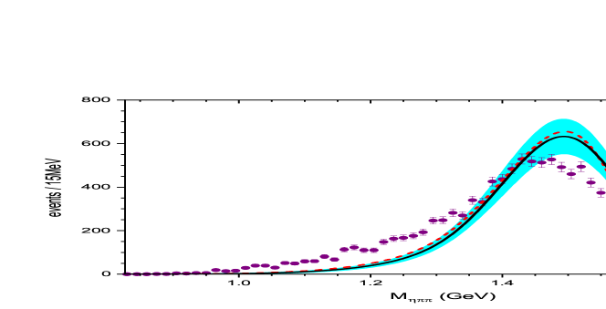
Figure 1: The prediction of $\tau^{-}\to\eta\pi^{-}\pi^{0}\nu_{\tau}$ from $e^{+}e^{-}\to\eta\pi^{+}\pi^{-}$ amplitudes. The black solid line is calculated from Fit II of Ref. [37] and the red dashed line is from Fit 4 of Ref. [36]. The cyan band describes the uncertainty obtained by a combined statistics of the error band of Fit II in Ref. [37] and the difference between the red and black lines. Belle data are represented by purple dots.

It can be seen that the prediction from $e^{+}e^{-}\to\eta\pi^{+}\pi^{-}$ is quite different from that of the Belle data [27], especially in the region of 0.9-1.4 GeV. The $\tau\to\eta\pi^{-}\pi^{0}\nu_{\tau}$ branching ratio is $(1.71\pm 0.13)\times 10^{-3}$, using the Fit II in Ref. [37], and $(1.55\pm 0.18)\times 10^{-3}$ from Fit 4 of Ref. [36]. The PDG quotes $(1.39\pm 0.07)\times 10^{-3}$ instead, from which our previous numbers are $2.2$ and $0.8$ $\sigma$ away, respectively. Meanwhile, $e^{+}e^{-}\to\eta\pi^{+}\pi^{-}$ data are considered much more accurate and trustworthy. Hence, it would be rather important for Belle-II to improve the measurement of this decay channel in the future.

The effects of NSI are constrained thanks to the most recent determination (in agreement with previous ones) of these couplings [46], yielding

$$\begin{pmatrix}\epsilon^{\tau}_{L}-\epsilon^{e}_{L}+\epsilon^{\tau}_{R}-\epsilon^{e}_{R}\\ \epsilon^{\tau}_{R}\\ \epsilon^{\tau}_{P}\\ \epsilon^{\tau}_{T}\\ \end{pmatrix}=\begin{pmatrix}2.4\pm 2.6\\ 0.7\pm 1.4\\ 0.4\pm 1.0\\ -3.3\pm 6.0\\ \end{pmatrix}\cdot 10^{-2}\,,$$ (21)

with the correlation matrix

$$C_{\epsilon}=\begin{pmatrix}1&0.87&-0.18&-0.98\\ &1&-0.59&-0.86\\ &&1&0.18\\ &&&1\\ \end{pmatrix}\,.$$ (22)

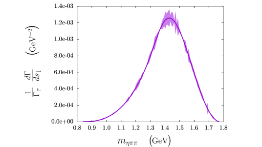
Figure 2: Invariant mass spectrum of the $\tau^{-}\to\eta\pi^{-}\pi^{0}\nu_{\tau}$ transition. The purple stripe is the error band obtained from the Gaussian variation of parameters at each bin, the solid purple line represents the mean of the distribution.

In our numerical analysis we used 2500 points generated randomly following a Gaussian distribution using the parameters and errors in eq. (21) and the correlation matrix of eq. (22). The vector form factor in ref. [25] was used in the following.

We also computed the invariant mass $m_{\eta\pi\pi}$ spectrum for which we again used a Gaussian variation of the parameters, generating 2500 points at each bin of the spectrum, shown in figure 2.

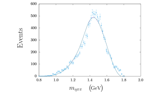
Figure 3: Comparison between the spectra obtained using the complete amplitude (purple line) with the NSI turned off (green line) and the Belle data (pale blue dots). The difference between both lines can be slightly appreciated only near the peak.

When comparing the result of the total differential decay width to that obtained only from the SM contribution to the amplitude and the Belle spectrum, shown in Figure 3, we confirm that the possible NSI contribution is undetectable with current data. In Fig. 4 we show a close up of the region where both curves of Fig. 3 differ a bit more.

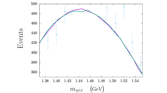
Figure 4: Close up of Figure 3 in the small region where they differ.

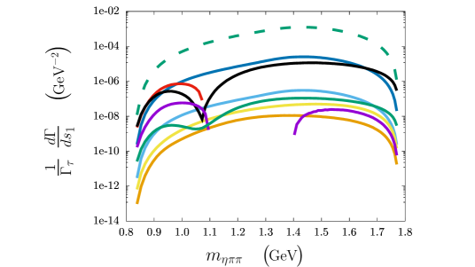
Figure 5: Different contributions to the differential decay width, shown in a logarithmic scale. Because of this, some of them cannot be shown in this figure, since interference terms are negative in certain regions of the invariant mass range. The color code follows: pure SM - dark green, SM-V - dark blue, SM-A - red, SM-T - black, A-V - lilac, V-T - green, A-T purple, $|$V$|^{2}$ - pale blue, $|$A$|^{2}$ - yellow, $|$T$|^{2}$ orange.

We also obtained the contributions to the decay width from the different terms in the squared amplitude, this is, pure $V$, $A$, $P$, $T$, SM terms or only one of the interference terms among them, in turn. This is shown in Figure 5 in a logarithmic scale. In Fig. 6 we show all such contributions, except for the pure SM one, in a normal scale. For most of the phase space the interference of the SM with the vector non-SM interaction dominates. At low invariant masses there is a small window where the SM-tensor and SM-axial interferences overcome it slightly. It is also seen that the SM-tensor interference dominates near the endpoint. It must be noted, however, that the tensor effects at high invariant masses may be smaller than depicted, as we are using for this form factor only the leading order contribution in the chiral expansion. Going beyond this approximation should -in particular- reduce the effects shown for the SM-tensor interference at high $m_{\eta\pi\pi}$. These results can be used to study possible new physics effects in the $\tau^{-}\to\eta\pi^{-}\pi^{0}\nu_{\tau}$ decays with future improved data.

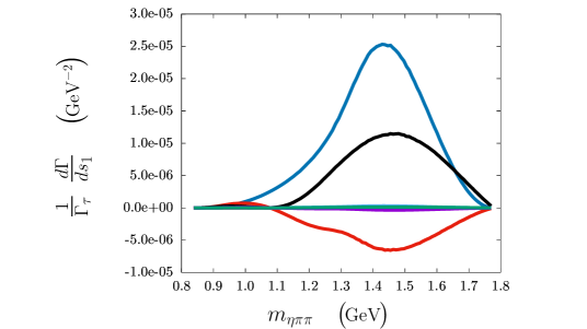
Figure 6: Same contributions from Figure 5, without the SM contribution. The color code is the same as in the previous figure.

5 Conclusions

We have studied whether the discrepancy between isospin-rotated $\sigma(e^{+}e^{-}\to\eta\pi^{+}\pi^{-})$ and $d\Gamma(\tau^{-}\to\eta\pi^{+}\pi^{0}\nu_{\tau})/dm_{\eta\pi\pi}$ data can be explained by heavy new physics beyond the SM. Within an effective field theory approach for the NSI (assuming left-handed neutrinos), and using the bounds obtained previously on the corresponding new physics couplings, we have shown that it is impossible to explain this tension between $e^{+}e^{-}$ and $\tau$ data by heavy new physics. Future measurement of the $\tau$ decay channel at Belle-II will shed light on the origin of this controversy. As a by-product of our analysis, we have developed the formalism needed to study NSI in three-meson tau decays (see ancillary file), which can be useful for other decay channels where hadronization is more complicated.

Appendix: Brief overview of Resonance Chiral Theory

In this appendix we recapitulate briefly the framework in which the model-dependent contributions have been evaluated [36, 37, 25], Resonance Chiral Theory (R$\chi$T) [72]. See, for instance ref. [95] for further details.

Resonances are added as explicit degrees of freedom to the $\chi$PT Lagrangian, which is enlarged by terms including them , where the $\chi$PT chiral tensors also appear. The symmetries determining the Lagrangian operators are the chiral one for the lightest pseudoscalar mesons (which are pseudoGoldstone bosons) and unitary symmetry for the resonances, $SU(3)_{L}\otimes SU(3)_{R}\to SU(3)_{V}$ and $U(3)_{V}$, respectively, for the three lightest quark flavors. The expansion parameter of R$\chi$T is the inverse of the number of colors [96], where the leading order corresponds to tree level diagrams with an infinite tower of mesons per quantum number [96, 97] (the most important subleading correction comes from finite resonance widths).

Symmetries do not restrict the coupling values, so these should in principle be determined phenomenologically. However, assuming that the theory with resonances can interpolate between the chiral and parton regimes, Green functions in R$\chi$T need to comply with the known (from the corresponding operator product expansion) QCD short-distance behaviour. This determines or relates some of the couplings, increasing the predictivity of R$\chi$T. At the same time, this requirement tightly constrains contributions from operators with high-order chiral tensors. Complementary, the number of resonance fields is limited by the process at hand (via the number of initial and final state mesons, to which exchanged resonances couple). Altogether, this restricts, in practice, the number of operators of the R$\chi$T Lagrangians in the large-$N_{C}$ limit. The minimal interactions with (pseudo)scalar and (axial)vector resonances are given by [72]

$$\mathcal{L}_{V} = \frac{F_{V}}{2\sqrt{2}}\left\langle V_{\mu\nu}f_{+}^{\mu\nu}\right\rangle+i\frac{G_{V}}{\sqrt{2}}\left\langle V_{\mu\nu}u^{\mu}u^{\nu}\right\rangle\,,\;\mathcal{L}_{A}\,=\,\frac{F_{A}}{2\sqrt{2}}\left\langle A_{\mu\nu}f_{-}^{\mu\nu}\right\rangle\,,$$

$$\mathcal{L}_{S} = c_{d}\left\langle Su^{\mu}u_{\mu}\right\rangle+c_{m}\left\langle S\chi_{+}\right\rangle\,,\;\mathcal{L}_{P}\,=\,id_{m}\left\langle P\chi_{-}\right\rangle\,,$$ (23)

see ref. [72] for further details.

Recent applications of R$\chi$T include refs. [80, 98, 99, 8, 37, 100, 44, 101, 45, 102], mostly focused on tau decays and hadronic contributions to the muon g-2.

References

- [1] S. I. Eidelman and V. N. Ivanchenko, Phys. Lett. B 257 (1991), 437-440.
- [2] R. Alemany, M. Davier and A. Höcker, Eur. Phys. J. C 2 (1998), 123-135.
- [3] V. Cirigliano, G. Ecker and H. Neufeld, Phys. Lett. B 513 (2001), 361-370.
- [4] V. Cirigliano, G. Ecker and H. Neufeld, JHEP 08 (2002), 002.
- [5] M. Davier, A. Hoecker, G. López Castro, B. Malaescu, X. H. Mo, G. Toledo Sánchez, P. Wang, C. Z. Yuan and Z. Zhang, Eur. Phys. J. C 66 (2010), 127-136.
- [6] M. Davier, A. Hoecker, B. Malaescu and Z. Zhang, Eur. Phys. J. C 71 (2011), 1515 [erratum: Eur. Phys. J. C 72 (2012), 1874].
- [7] M. Davier, A. Höcker, B. Malaescu, C. Z. Yuan and Z. Zhang, Eur. Phys. J. C 74 (2014) no.3, 2803.
- [8] J. A. Miranda and P. Roig, Phys. Rev. D 102 (2020), 114017.
- [9] M. Benayoun, L. DelBuono and F. Jegerlehner, Eur. Phys. J. C 82 (2022) no.2, 184.
- [10] T. Aoyama, N. Asmussen, M. Benayoun, J. Bijnens, T. Blum, M. Bruno, I. Caprini, C. M. Carloni Calame, M. Cè and G. Colangelo, et al. Phys. Rept. 887 (2020), 1-166.
- [11] M. Davier, A. Hoecker, B. Malaescu and Z. Zhang, Eur. Phys. J. C 77 (2017) no.12, 827.
- [12] A. Keshavarzi, D. Nomura and T. Teubner, Phys. Rev. D 97 (2018) no.11, 114025.
- [13] G. Colangelo, M. Hoferichter and P. Stoffer, JHEP 02 (2019), 006.
- [14] M. Hoferichter, B. L. Hoid and B. Kubis, JHEP 08 (2019), 137.
- [15] M. Davier, A. Hoecker, B. Malaescu and Z. Zhang, Eur. Phys. J. C 80 (2020) no.3, 241 [erratum: Eur. Phys. J. C 80 (2020) no.5, 410].
- [16] A. Keshavarzi, D. Nomura and T. Teubner, Phys. Rev. D 101 (2020) no.1, 014029.
- [17] G. Colangelo, M. Davier, A. X. El-Khadra, M. Hoferichter, C. Lehner, L. Lellouch, T. Mibe, B. L. Roberts, T. Teubner and H. Wittig, et al., [arXiv:2203.15810 [hep-ph]].
- [18] S. Borsanyi, Z. Fodor, J. N. Guenther, C. Hoelbling, S. D. Katz, L. Lellouch, T. Lippert, K. Miura, L. Parato and K. K. Szabo, et al. Nature 593 (2021) no.7857, 51-55.
- [19] M. Cè, A. Gérardin, G. von Hippel, R. J. Hudspith, S. Kuberski, H. B. Meyer, K. Miura, D. Mohler, K. Ottnad and P. Srijit, et al. [arXiv:2206.06582 [hep-lat]].
- [20] C. Alexandrou, S. Bacchio, P. Dimopoulos, J. Finkenrath, R. Frezzotti, G. Gagliardi, M. Garofalo, K. Hadjiyiannakou, B. Kostrzewa and K. Jansen, et al. [arXiv:2206.15084 [hep-lat]].
- [21] B. Abi et al. [Muon g-2], Phys. Rev. Lett. 126 (2021) no.14, 141801.
- [22] G. W. Bennett et al. [Muon g-2], Phys. Rev. D 73 (2006), 072003.
- [23] Y. S. Tsai, Phys. Rev. D 4 (1971) 2821 Erratum: [Phys. Rev. D 13 (1976) 771].
- [24] V. Cherepanov and S. Eidelman, Nucl. Phys. Proc. Suppl. 218 (2011) 231.
- [25] D. Gómez Dumm and P. Roig, Phys. Rev. D 86 (2012) 076009.
- [26] P. Roig, [arXiv:1301.7626 [hep-ph]]. Ph. D. Thesis, Univ. Valéncia (2010).
- [27] K. Inami et al. [Belle], Phys. Lett. B 672 (2009), 209-218.
- [28] A. Antonelli et al. [DM2], Phys. Lett. B 212 (1988), 133-138.
- [29] S. I. Dolinsky, V. P. Druzhinin, M. S. Dubrovin, V. B. Golubev, V. N. Ivanchenko, E. V. Pakhtusova, A. N. Peryshkin, S. I. Serednyakov, Y. M. Shatunov and V. A. Sidorov, et al. Phys. Rept. 202 (1991), 99-170.
- [30] R. R. Akhmetshin et al. [CMD-2], Phys. Lett. B 489 (2000), 125-130.
- [31] B. Aubert et al. [BaBar], Phys. Rev. D 76 (2007), 092005 [erratum: Phys. Rev. D 77 (2008), 119902].
- [32] V. M. Aulchenko et al. [SND], Phys. Rev. D 91 (2015) no.5, 052013.
- [33] M. N. Achasov, V. M. Aulchenko, A. Y. Barnyakov, K. I. Beloborodov, A. V. Berdyugin, D. E. Berkaev, A. G. Bogdanchikov, A. A. Botov, T. V. Dimova and V. P. Druzhinin, et al. Int. J. Mod. Phys. Conf. Ser. 35 (2014), 1460388.
- [34] M. N. Achasov, A. Y. Barnyakov, K. I. Beloborodov, A. V. Berdyugin, D. E. Berkaev, A. G. Bogdanchikov, A. A. Botov, T. V. Dimova, V. P. Druzhinin and V. B. Golubev, et al. Phys. Rev. D 97 (2018) no.1, 012008.
- [35] S. S. Gribanov, A. S. Popov, R. R. Akhmetshin, A. N. Amirkhanov, A. V. Anisenkov, V. M. Aulchenko, V. S. Banzarov, N. S. Bashtovoy, D. E. Berkaev and A. E. Bondar, et al. JHEP 01 (2020), 112.
- [36] L. Y. Dai, J. Portolés and O. Shekhovtsova, Phys. Rev. D 88 (2013), 056001.
- [37] W. Qin, L. Y. Dai and J. Portolés, JHEP 03 (2021) 092.
- [38] E. A. Garcés, M. Hernández Villanueva, G. López Castro and P. Roig, JHEP 12 (2017), 027.
- [39] J. A. Miranda and P. Roig, JHEP 11 (2018), 038.
- [40] V. Cirigliano, A. Falkowski, M. González-Alonso and A. Rodríguez-Sánchez, Phys. Rev. Lett. 122 (2019) no.22, 221801.
- [41] J. Rendón, P. Roig and G. Toledo Sánchez, Phys. Rev. D 99 (2019) no.9, 093005.
- [42] S. Gonzàlez-Solís, A. Miranda, J. Rendón and P. Roig, Phys. Rev. D 101 (2020) no.3, 034010.
- [43] S. Gonzàlez-Solís, A. Miranda, J. Rendón and P. Roig, Phys. Lett. B 804 (2020), 135371.
- [44] M. A. Arroyo-Ureña, G. Hernández-Tomé, G. López-Castro, P. Roig and I. Rosell, Phys. Rev. D 104 (2021) no.9, L091502.
- [45] M. A. Arroyo-Ureña, G. Hernández-Tomé, G. López-Castro, P. Roig and I. Rosell, JHEP 02 (2022), 173.
- [46] V. Cirigliano, D. Díaz-Calderón, A. Falkowski, M. González-Alonso and A. Rodríguez-Sánchez, JHEP 04 (2022), 152.
- [47] E. Kou et al. [Belle-II], PTEP 2019 (2019) no.12, 123C01 [erratum: PTEP 2020 (2020) no.2, 029201].
- [48] S. Descotes-Genon and B. Moussallam, Eur. Phys. J. C 74 (2014), 2946.
- [49] R. Escribano, S. Gonzàlez-Solís and P. Roig, Phys. Rev. D 94 (2016) no.3, 034008.
- [50] V. Cirigliano, J. Jenkins and M. González-Alonso, Nucl. Phys. B 830 (2010), 95-115.
- [51] T. Bhattacharya, V. Cirigliano, S. D. Cohen, A. Filipuzzi, M. González-Alonso, M. L. Graesser, R. Gupta and H. W. Lin, Phys. Rev. D 85 (2012), 054512.
- [52] V. Cirigliano, M. González-Alonso and M. L. Graesser, JHEP 02 (2013), 046.
- [53] V. Cirigliano, S. Gardner and B. Holstein, Prog. Part. Nucl. Phys. 71 (2013), 93-118.
- [54] H. M. Chang, M. González-Alonso and J. Martín Camalich, Phys. Rev. Lett. 114 (2015) no.16, 161802.
- [55] A. Courtoy, S. Baeßler, M. González-Alonso and S. Liuti, Phys. Rev. Lett. 115 (2015), 162001.
- [56] M. González-Alonso and J. Martín Camalich, JHEP 12 (2016), 052.
- [57] M. González-Alonso, J. Martín Camalich and K. Mimouni, Phys. Lett. B 772 (2017), 777-785.
- [58] S. Alioli, V. Cirigliano, W. Dekens, J. de Vries and E. Mereghetti, JHEP 05 (2017), 086.
- [59] M. González-Alonso, O. Naviliat-Cuncic and N. Severijns, Prog. Part. Nucl. Phys. 104 (2019), 165-223.
- [60] S. Descotes-Genon, A. Falkowski, M. Fedele, M. González-Alonso and J. Virto, JHEP 05 (2019), 172.
- [61] V. Cirigliano, A. Crivellin and M. Hoferichter, Phys. Rev. Lett. 120 (2018) no.14, 141803.
- [62] F. Z. Chen, X. Q. Li, Y. D. Yang and X. Zhang, Phys. Rev. D 100 (2019) no.11, 113006.
- [63] F. Z. Chen, X. Q. Li and Y. D. Yang, JHEP 05 (2020), 151.
- [64] F. Z. Chen, X. Q. Li, S. C. Peng, Y. D. Yang and H. H. Zhang, JHEP 01 (2022), 108.
- [65] W. Buchmuller and D. Wyler, Nucl. Phys. B 268 (1986), 621-653.
- [66] B. Grzadkowski, M. Iskrzynski, M. Misiak and J. Rosiek, JHEP 10 (2010), 085.
- [67] R. Kumar, Phys. Rev. 185 (1969), 1865-1875.
- [68] S. Arteaga, “Effective field theory analysis of the decays”, Master Thesis, October 2019, Cinvestav.
- [69] N. N. Achasov, S. A. Devyanin and G. N. Shestakov, Phys. Lett. 88B (1979) 367.
- [70] S. Jadach, Z. Was, R. Decker and J. H. Kühn, Comput. Phys. Commun. 76 (1993), 361-380.
- [71] S. Actis et al. [Working Group on Radiative Corrections and Monte Carlo Generators for Low Energies], Eur. Phys. J. C 66 (2010) 585.
- [72] G. Ecker, J. Gasser, A. Pich and E. de Rafael, Nucl. Phys. B 321 (1989) 311. G. Ecker, J. Gasser, H. Leutwyler, A. Pich and E. de Rafael, Phys. Lett. B 223 (1989) 425.
- [73] M. Jamin, J. A. Oller and A. Pich, Nucl. Phys. B 587 (2000), 331-362.
- [74] M. Jamin, J. A. Oller and A. Pich, Nucl. Phys. B 622 (2002), 279-308.
- [75] R. Escribano, P. Masjuan and J. J. Sanz-Cillero, JHEP 1105 (2011) 094.
- [76] C. Hanhart, B. Kubis and J. R. Peláez, Phys. Rev. D 76 (2007) 074028.
- [77] P. A. Zyla et al. [Particle Data Group], PTEP 2020 (2020) no.8, 083C01.
- [78] V. Cirigliano, G. Ecker, H. Neufeld and A. Pich, JHEP 0306 (2003) 012.
- [79] J. Schechter, A. Subbaraman and H. Weigel, Phys. Rev. D 48 (1993) 339. T. Feldmann and P. Kroll, Eur. Phys. J. C 5 (1998) 327; Phys. Scripta T 99 (2002) 13. T. Feldmann, P. Kroll and B. Stech, Phys. Rev. D 58 (1998) 114006; Phys. Lett. B 449 (1999) 339. T. Feldmann, Int. J. Mod. Phys. A 15 (2000) 159. R. Escribano and J. M. Frere, Phys. Lett. B 459 (1999) 288; JHEP 0506 (2005) 029.
- [80] A. Guevara, P. Roig and J. J. Sanz-Cillero, JHEP 06 (2018), 160.
- [81] P. Roig, A. Guevara and G. López Castro, Phys. Rev. D 89 (2014) no.7, 073016.
- [82] F. Ambrosino et al., JHEP 0907, 105 (2009).
- [83] D. G. Dumm, P. Roig, A. Pich and J. Portolés, Phys. Lett. B 685 (2010) 158.
- [84] O. Shekhovtsova, T. Przedzinski, P. Roig and Z. Was, Phys. Rev. D 86 (2012) 113008
- [85] I. M. Nugent, T. Przedzinski, P. Roig, O. Shekhovtsova and Z. Was, Phys. Rev. D 88 (2013) 093012.
- [86] D. G. Dumm, P. Roig, A. Pich and J. Portolés, Phys. Rev. D 81 (2010) 034031.
- [87] S. Weinberg, Physica A 96 (1979) no.1-2, 327-340. J. Gasser and H. Leutwyler, Annals Phys. 158 (1984), 142; Nucl. Phys. B 250 (1985), 465-516.
- [88] O. Catà and V. Mateu, JHEP 09 (2007), 078.
- [89] I. Baum, V. Lubicz, G. Martinelli, L. Orifici and S. Simula, Phys. Rev. D 84 (2011), 074503.
- [90] V. Shtabovenko, R. Mertig and F. Orellana, Comput. Phys. Commun. 256 (2020), 107478
- [91] V. Shtabovenko, R. Mertig and F. Orellana, Comput. Phys. Commun. 207 (2016), 432-444
- [92] R. Mertig, M. Bohm and A. Denner, Comput. Phys. Commun. 64 (1991), 345-359
- [93] M. K. Volkov, A. B. Arbuzov and D. G. Kostunin, Phys. Rev. C 89 (2014) no.1, 015202.
- [94] A. Sirlin, Nucl. Phys. B 71 (1974) 29; Rev. Mod. Phys. 50 (1978) 573 Erratum: [Rev. Mod. Phys. 50 (1978) 905]; Nucl. Phys. B 196 (1982) 83. W. J. Marciano and A. Sirlin, Phys. Rev. Lett. 56 (1986) 22; Phys. Rev. Lett. 61, 1815 (1988); Phys. Rev. Lett. 71 (1993) 3629. J. Erler, Rev. Mex. Fis. 50 (2004) 200.
- [95] V. Cirigliano, G. Ecker, M. Eidemüller, R. Kaiser, A. Pich and J. Portolés, Nucl. Phys. B 753 (2006), 139-177.
- [96] G. ’t Hooft, Nucl. Phys. B 72 (1974), 461.
- [97] G. ’t Hooft, Nucl. Phys. B 75 (1974), 461-470.
- [98] L. Y. Dai, J. Fuentes-Martín and J. Portolés, Phys. Rev. D 99 (2019) no.11, 114015.
- [99] P. Roig and P. Sánchez-Puertas, Phys. Rev. D 101 (2020) no.7, 074019.
- [100] J. L. Gutiérrez Santiago, G. López Castro and P. Roig, Phys. Rev. D 103 (2021) no.1, 014027.
- [101] A. Guevara, G. L. Castro and P. Roig, Phys. Rev. D 105 (2022) no.7, 076007.
- [102] C. Chen, C. G. Duan and Z. H. Guo, JHEP 08 (2022), 144.