Next-to-next-to-leading order matching of beauty-charmed meson $B_{c}$ and $B^{*}_{c}$ decay constants

Abstract

We present the next-to-next-to-leading order (NNLO) QCD corrections to the decay constants for both the pseudoscalar and vector beauty-charmed mesons $B_{c}$ and $B^{*}_{c}$ in nonrelativistic QCD effective theory. Explicit NNLO calculation verified that the $B_{c}$ decay constant from pseudoscalar current is identical with the $B_{c}$ decay constant from axial-vector current. The NNLO result for the vector decay constant of $B^{*}_{c}$ meson is novel. Combined with the latest extraction of nonrelativistic QCD long-distance matrix elements of $B_{c}$ meson, we give the branching ratios of leptonic decays of $B_{c}$ and $B^{*}_{c}$ mesons. In addition, the novel anomalous dimension for the flavor-changing heavy quark vector current in nonrelativistic QCD effective theory are helpful to investigate the threshold behaviours of two different heavy quarks.

I Introduction

The beauty-charmed meson $B_{c}(1S)$ was first discovered in proton anti-proton colliders by CDF collaboration in 1998 CDF:1998ihx . The second new member in beauty-charmed meson family, i.e. $B_{c}(2S)$, was discovered in proton proton colliders by ATLAS collaboration in 2014 ATLAS:2014lga . Five years later, the $B_{c}(2S)$ state was confirmed by both CMS and LHCb collaborations, in addition, the new vector member $B^{*}_{c}(2S)$ was first reported by these two collaborations CMS:2019uhm ; LHCb:2019bem . Up to now, no other member in beauty-charmed meson family is observed in particle physics experiment though more beauty-charmed mesons have been predicted in many theoretical models.

Unlike the heavy quarkonium, the experimental measurements of beauty-charmed meson family are not easy since they are composed of two different heavy flavor quarks and the ground state $B_{c}(1S)$ only weak decays into other lighter particles. Though there are 48 decay channels listed in latest review of particle physics which have been reported in experiments, no one has an experimental measurement of absolute branching ratios  Workman:2022ynf .

To promote the determination of the absolute branching ratios, it is required to carefully investigate the fundamental properties of decay behaviours. In other words, we need first to have a good knowledge of the decay constants for the beauty-charmed meson family. In principle, the decay constants for the beauty-charmed mesons are nonperturbative yet universal physical quantities. In this point Lattice QCD shall be a good method to determine the decay constants from the first principal of QCD. However, the Lattice QCD studies on the beauty-charmed mesons are lesser because the beauty-charmed mesons include two different heavy quarks and the doubly heavy quark systems are not easy to be simulated in current lattices.

The nonrelativistic QCD (NRQCD) effective theory provides a systematical and accurate framework to study the doubly heavy quark systems Bodwin:1994jh . In this effective theory, the heavy quark mass provides a nature factorization scale. The short-distance physics above the heavy quark mass can be perturbatively calculated and factorized into the Wilson coefficients while the long-distance physics below the heavy quark mass go into the long-distance matrix elements (LDMEs). Within NRQCD effective theory, the decay constants for beauty-charmed mesons can be further factorized as the short-distance matching coefficients and the corresponding NRQCD LDMEs.

Using NRQCD effective theory, the next-to-leading order (NLO) corrections including both the strong coupling constant correction at order $\alpha_{s}$ and relative velocity correction at order $v^{2}$ to the axial-vector decay constant of the $B_{c}$ meson was first calculated by Braaten and Fleming in 1995 Braaten:1995ej , after a systematical study of the $B_{c}$ meson at the leading order (LO) by Chang and Chen Chang:1992pt . Using the resummation technique, the NLO corrections including all order relative velocity corrections to the axial-vector decay constant of $B_{c}$ meson and the vector decay constant of $B^{*}_{c}$ was estimated by Lee, Sang, and Kim in 2010 Lee:2010ts . The next-to-next-to-leading order (NNLO) corrections at order $\alpha^{2}_{s}$ to the axial-vector decay constant of $B_{c}$ meson was first investigated by Onishchenko and Veretin in 2003 Onishchenko:2003ui . However, the full analytical expression of the axial-vector decay constant of $B_{c}$ meson at NNLO accuracy was accomplished by Chen and Qiao in 2015 Chen:2015csa . Very recently, the numerical calculation of the axial-vector decay constant of $B_{c}$ meson at NNNLO accuracy was by Feng, Jia, Mo, Pan, Sang, and Zhang Feng:2022ruy . Other higher-order calculation on doubly heavy quark system and phenomenological studies on $B_{c}$ system can be found, for example, in the literatures Marquard:2006qi ; Egner:2021lxd ; Beneke:1997jm ; Marquard:2009bj ; Marquard:2014pea ; Kniehl:2002yv ; Egner:2022jot ; Sang:2022kub ; Feng:2022vvk ; Chen:2022vzo ; Chen:2017soz ; Tao:2022yur ; Tang:2022nqm ; Zhu:2017lwi ; Zhu:2017lqu ; Zhao:2022auq ; Bordone:2022drp ; Sun:2022hyk ; Xiao:2013lia ; Wang:2012kw ; Piclum:2007an .

In this paper, we will calculate the pseudoscalar decay constant of $B_{c}$ meson and the vector decay constant of $B^{*}_{c}$ meson at NNLO accuracy within NRQCD effective theory. By an explicit calculation, we can investigate the relation among various decay constants defined by different flavor-changing heavy quark currents. The pseudoscalar decay constant of $B_{c}$ meson is identical to the axial-vector decay constant of $B_{c}$ meson. The NNLO results of the vector decay constant of $B^{*}_{c}$ meson are novel. Combined with the latest extraction of the NRQCD LDMEs, we give the branching ratios of leptonic decays of $B_{c}$ and $B^{*}_{c}$ mesons. These results of matching coefficients are also useful to analyze the threshold behaviours when two different heavy quark are close to each other.

In addition, we obtain a novel anomalous dimension for the flavor-changing heavy quark vector current at NNLO accuracy of NRQCD effective theory. This anomalous dimension is related to the renormalization behaviours of the vector current with two different heavy quarks in NRQCD.

The paper is arranged as follows. In Sec. II, we give the definition of the decay constants from pseudoscalar, axial-vector, and vector currents for beauty-charmed mesons $B_{c}$ and $B^{*}_{c}$ in both the full QCD theory and the NRQCD effective theory. We then present the matching formulae for the decay constants in the NRQCD effective theory. In Sec. III, we present the calculation methods and calculation procedures for the short-distance matching coefficients. In Sec. IV, we give the final NNLO results of the short-distance matching coefficients and the decay constants of $B_{c}$ and $B^{*}_{c}$. We also perform a phenomenological analysis of the leptonic decays of $B_{c}$ and $B^{*}_{c}$. We conclude in the end of the paper.

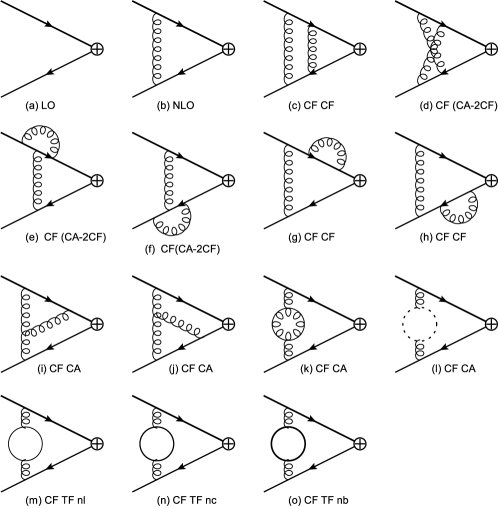
Figure 1: The Feynman diagrams labelled with corresponding color factor for $B_{c}$ and $B^{*}_{c}$ decay constants up to two-loop order. The cross “$\bigoplus$” implies the insertion of certain heavy flavor-changing current. The thinnest, thick, thickest solid circles represent $n_{l}$ massless quark-loop, $n_{c}$ quark-loop with mass $m_{c}$, $n_{b}$ quark-loop with mass $m_{b}$, respectively. In this paper, $n_{b}=n_{c}=1$.

II Matching formulae

Though the $B_{c}$ meson leptonic decay is dominated by the virtual $W$ boson with a $V-A$ weak interaction in particle physics standard model, one can freely define the $B_{c}$ meson decay constants by different flavor-changing currents. Thus one can define the pseudoscalar and vector $B_{c}$ meson decay constants by the full QCD matrix elements

$$\left\langle 0\left|\bar{b}\gamma^{\mu}\gamma_{5}c\right|B_{c}(P)\right\rangle =if^{a}_{B_{c}}P^{\mu},$$ (1)

$$\left\langle 0\left|\bar{b}\gamma_{5}c\right|B_{c}(P)\right\rangle =if^{p}_{B_{c}}m_{B_{c}},$$ (2)

$$\left\langle 0\left|\bar{b}\gamma^{\mu}c\right|B^{*}_{c}(P,\varepsilon)\right\rangle =f^{v}_{B^{*}_{c}}m_{B^{*}_{c}}\varepsilon^{\mu},$$ (3)

where $\left|B_{c}(P)\right\rangle$ and $\left|B^{*}_{c}(P,\varepsilon)\right\rangle$ are respectively the states of pseudoscalar and vector $B_{c}$ mesons with four-momentum $P$ and $\varepsilon^{\mu}$ is the polarization vector for vector $B_{c}$ meson. In full QCD, the standard covariant normalization of the hadron state is $\left\langle B_{c}\left(P^{\prime}\right)\mid B_{c}(P)\right\rangle=(2\pi)^{3}2P^{0}\delta^{3}\left(P^{\prime}-P\right)$. The imaginary unit in the right hand of equations is added to make sure the $f_{B_{c}}$ being real and positive. Note that other decay constants for $B_{c}$ family with scalar and tensor currents are not considered in this paper. Using the heavy quark equation of motion, one can easily get the identity $f^{a}_{B_{c}}=f^{p}_{B_{c}}$. Thus we only need to calculate two decay constants $f^{p}_{B_{c}}$ and $f^{v}_{B^{*}_{c}}$ in the following.

The above decay constants of $B_{c}$ mesons are principally nonperturbative observables in full QCD and rely on a nonperturbative calculation, however, the two heavy quark system is not well-simulated at current Lattice QCD and these physical quantities are rarely investigated in the first principal theory of QCD.

In NRQCD effective theory, the decay constants of $B_{c}$ mesons can be further factorized into a perturbatively calculable short-distance coefficients with the corresponding nonperturbative LDMEs. Thus one can write the following matching formula at leading-order in relative velocity expansion

$$f^{p}_{B_{c}} =\sqrt{\frac{2}{m_{B_{c}}}}\mathcal{C}_{p}(m_{b},m_{c},\mu_{f})\left\langle 0\left|\chi^{\dagger}_{b}\psi_{c}\right|B_{c}(\mathbf{P})\right\rangle(\mu_{f})+{\cal O}(v^{2}),$$ (4)

$$f^{v}_{B^{*}_{c}} =\sqrt{\frac{2}{m_{B^{*}_{c}}}}\mathcal{C}_{v}(m_{b},m_{c},\mu_{f})\left\langle 0\left|\chi^{\dagger}_{b}\mathbf{\sigma}\psi_{c}\right|B^{*}_{c}(\mathbf{P})\right\rangle(\mu_{f})+{\cal O}(v^{2}),$$ (5)

where $\mu_{f}$ is the NRQCD factorization scale which appears in the short-distance coefficients at two-loop calculation and will be cancelled between the short-distance coefficients and NRQCD LDMEs. In QCD perturbative calculation, the decay constants will depend on the renormalization scale in fixed-order accuracy and will become renormalization scale independence after summing all-order contributions.

III Calculation of the matching coefficients

In this section, we present our calculation procedures for the decay constants of pseudoscalar and vector $B_{c}$ mesons within NRQCD approach. According to the above matching formulae, the matching coefficients $\mathcal{C}_{p}$ and $\mathcal{C}_{v}$ can be obtained by the calculation of both full QCD matrix elements and the NRQCD matrix elements. At leading-order, the matching coefficients $\mathcal{C}_{p}$ and $\mathcal{C}_{v}$ are set as $\mathcal{C}_{p}=\mathcal{C}_{v}=1$, which can also be done after the nonrelativistic expansion of heavy quark current. The Feynman diagrams for $B_{c}$ and $B^{*}_{c}$ decay constants up to two-loop order are plotted in Fig. 1.

Our higher order calculation of the matching coefficients consists of the following steps. First, we use FeynCalc Shtabovenko:2020gxv to obtain Feynman diagrams and corresponding Feynman amplitudes. By $Apart Feng:2012iq , we decompose every Feyman amplitude to several Feynman integral families. Second, we use Kira Klappert:2020nbg /FIRE Smirnov:2019qkx / FiniteFlow Peraro:2019svx based on Integration by Parts(IBP) Chetyrkin:1981qh to reduce every Feynman integral family to master integral family. Third, based on symmetry among different integral families and using Kira+FIRE+Mathematica code, we can realize integral reduction among different integral families, and further on, the reduction from all of master integral families to the minimal master integral families. Last, we use AMFlow Liu:2022chg , which is a proof-of-concept implementation of the auxiliary mass flow method Liu:2017jxz , equipped with Kira/FiniteFlow to calclate the minimal master integral families one by one.

In order to obtain the high-order coefficient $\mathcal{C}_{J}$ with $J=p,~{}v$, one has to perform the conventional renormalization procedure, which are similar to what are shown in Refs. Chen:2015csa ; Kniehl:2006qw ; Bonciani:2008wf ; Davydychev:1997vh , i.e., $Z_{J}Z_{2,b}^{\frac{1}{2}}Z_{2,c}^{\frac{1}{2}}\Gamma_{J}=\mathcal{C}_{J}\tilde{Z}^{-1}_{J}\tilde{Z}_{2,b}^{\frac{1}{2}}\tilde{Z}_{2,c}^{\frac{1}{2}}\tilde{\Gamma}_{J}$ where the left part in the equation represents the renormalization of full QCD current while the right part represents the renormalization of NRQCD current. $Z_{J}$ and $\tilde{Z}^{-1}_{J}$ are the renormalization constants for full QCD and NRQCD flavor-changing currents, respectively. Here, $Z_{a}=Z_{v}=1$, $Z_{p}=\frac{m_{b}Z_{m,b}+m_{c}Z_{m,c}}{m_{b}+m_{c}}$. And $\tilde{Z}_{2,b}=\tilde{Z}_{2,c}=\tilde{\Gamma}_{J}=1$. Equivalently, We can also use diagrammatic renormalization method deOliveira:2022eeq , which contain two loop diagrams and three kinds of counter-term diagrams, i.e., tree diagram inserted with one $\alpha_{s}^{2}$-order counter-term vertex, tree diagram inserted with two $\alpha_{s}$-order counter-term vertexes (vanishing), and one loop diagram inserted with one $\alpha_{s}$-order counter-term vertex.

We want to mention that all contributions have been evaluated for general gauge parameter $\xi$ and the final results for the matching coefficients are all independent of $\xi$, which constitutes an important check on our calculation. In the calculation of two loop diagrams, we allow for one $b$ quark, one $c$ quark and $n_{l}$ massless quarks in the quark loop. Up to two-loop order, the most complicated renormalization constants are the on-shell mass and wave function renormalization constants allowing for two different non-zero quark masses Bekavac:2007tk ; Fael:2020bgs , which are presented in the appendix.

After renormalization, the results of the short-distance matching coefficients $\mathcal{C}_{J}$ can be expressed as

$$\mathcal{C}_{J}(\mu_{f},\mu,m_{b},x)=$$

$$1+\frac{\alpha_{s}^{(n_{f})}}{\pi}\mathcal{C}_{J}^{(1)}(x)+\left(\frac{\alpha_{s}^{(n_{f})}}{\pi}\right)^{2}\left(\mathcal{C}_{J}^{(1)}(x)\frac{\beta_{0}^{(n_{f})}}{4}\text{ln}\frac{\mu^{2}}{m_{b}^{2}}+\frac{\gamma_{J}^{(2)}(x)}{2}\ln\frac{\mu_{f}^{2}}{m_{b}^{2}}\right.$$

$$\left.+C^{2}_{F}\mathcal{C}^{FF}_{J}(x)+C_{F}C_{A}\mathcal{C}^{FA}_{J}(x)+C_{F}T_{F}n_{l}\mathcal{C}^{FL}_{J}(x)+C_{F}T_{F}\mathcal{C}^{FH}_{J}(x)\right)$$

$$+\mathcal{O}(\alpha^{3}_{s}).$$ (6)

where we have defined a dimensionless parameter $x$ representing the ratio of two heavy quark masses

$$x={m_{c}\over m_{b}}.$$ (7)

Besides we have suppress the renormalization scale $\mu$ dependence in strong coupling constant $\alpha_{s}$. The first two coefficients in $\beta$ functions for $\alpha_{s}$ are

$$\beta_{0}^{(n_{f})}=(11/3)C_{A}-(4/3)T_{F}n_{f},$$ (8)

$$\beta_{1}^{(n_{f})}=(34/3)C_{A}^{2}-(20/3)C_{A}T_{F}n_{f}-4C_{F}T_{F}n_{f}.$$ (9)

If keeping the heavy quark mass in gluon self energies Feynman diagrams, the heavy quark mass will go into the running of the strong coupling constant. We apply the following decoupling relation Chetyrkin:2005ia ; Bernreuther:1981sg ; Barnreuther:2013qvf ; Grozin:2007fh ; Ozcelik:2021zqt to translate $\alpha_{s}^{(n_{f})}$ involving massive flavours to $\alpha_{s}^{(n_{l})}$ only involving $n_{l}$ massless flavours,

$$\frac{\alpha_{s}^{(n_{f})}}{\alpha_{s}^{(n_{l})}}=1+\frac{\alpha_{s}^{(n_{l})}}{\pi}T_{F}\left(\frac{n_{b}}{3}\text{ln}\frac{\mu^{2}}{m_{b}^{2}}+\frac{n_{c}}{3}\text{ln}\frac{\mu^{2}}{m_{c}^{2}}+\mathcal{O}(\epsilon)\right)+\mathcal{O}(\alpha^{2}_{s}),$$ (10)

where $n_{f}=n_{l}+n_{b}+n_{c}$. In our numerical calculation, $n_{b}=n_{c}=1$, $n_{l}=3$ and the two loop result for strong coupling constant Chetyrkin:1997sg ; Chetyrkin:2000yt ; Deur:2016tte ; Herren:2017osy is used, i.e.,

$$\alpha_{s}^{(n_{l})}\left(\mu\right)=\frac{4\pi}{\beta_{0}^{(n_{l})}\text{ln}\frac{\mu^{2}}{{\Lambda_{QCD}^{(n_{l})}}^{2}}}\left(1-\frac{\beta_{1}^{(n_{l})}\text{ln}\,\text{ln}\frac{\mu^{2}}{{\Lambda_{QCD}^{(n_{l})}}^{2}}}{{\beta_{0}^{(n_{l})}}^{2}\text{ln}\frac{\mu^{2}}{{\Lambda_{QCD}^{(n_{l})}}^{2}}}\right),$$ (11)

where the typical QCD scale $\Lambda_{QCD}^{(n_{l}=3)}=336\mathrm{MeV}$ can be iteratively determined by $\alpha_{s}^{(n_{l}=5)}(m_{Z})=0.1179$ with $m_{Z}=91.1876\mathrm{GeV}$.

Explicit analytical calculation of the NLO Feynman diagrams give the NLO short-distance matching coefficients

$$\mathcal{C}_{p}^{(1)}(x)=\frac{3}{4}C_{F}\left(\frac{x-1}{x+1}\text{ln}x-2\right),$$ (12)

$$\mathcal{C}_{v}^{(1)}(x)=\frac{3}{4}C_{F}\left(\frac{x-1}{x+1}\text{ln}x-\frac{8}{3}\right).$$ (13)

Note that the analytical expressions of $\mathcal{C}_{p}^{(1)}(x)$ and $\mathcal{C}_{v}^{(1)}(x)$ are consistent with previous literatures Braaten:1995ej ; Lee:2010ts .

At NNLO, the direct results of the matching coefficients are still IR-divergent after performing the UV renormalization. This is due to the UV divergence in the NRQCD LDMEs at NNLO. The anomalous dimensions $\gamma_{J}$ is related to $\tilde{Z}_{J}$ by

$$\gamma_{J}=\frac{\text{d}\ln\tilde{Z}_{J}}{\text{d}\ln\mu}|_{\epsilon=0}=\left(\frac{\alpha_{s}^{\left(n_{f}\right)}}{\pi}\right)^{2}\gamma_{J}^{(2)}(x)+\mathcal{O}(\alpha^{3}_{s}),$$ (14)

whose solution gives the renormalization constants $\tilde{Z}_{J}$ for different NRQCD currents

$$\tilde{Z}_{J}=1-\left(\frac{\alpha_{s}^{\left(n_{f}\right)}}{\pi}\right)^{2}\left(\frac{\mu^{2}}{\mu_{f}^{2}}\right)^{2\epsilon}\frac{\gamma_{J}^{(2)}(x)}{4\epsilon}+\mathcal{O}(\alpha^{3}_{s}),$$ (15)

where

$$\gamma_{p}^{(2)}(x)=-\pi^{2}\left(\frac{C_{F}C_{A}}{2}+\frac{(1+6x+x^{2})C_{F}^{2}}{2(1+x)^{2}}\right),$$ (16)

$$\gamma_{v}^{(2)}(x)=-\pi^{2}\left(\frac{C_{F}C_{A}}{2}+\frac{(3+2x+3x^{2})C_{F}^{2}}{6(1+x)^{2}}\right).$$ (17)

Note that the anomalous dimension $\gamma_{v}^{(2)}(x)$ is a novel result for two different heavy quarks meson. In the case of $x=1$, the result is consistent with the previous calculation, for example in Ref. Kniehl:2006qw . By the renormalization of the the UV divergence in the NRQCD LDMEs at NNLO, the extra IR-divergences in short-distance coefficients can be exactly cancelled. Thus we finally get the finite results for the matching coefficients.

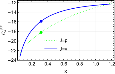
Figure 2: The profile of sub-coefficient $\mathcal{C}^{FF}_{J}(x)$ dependence on heavy quark mass ratio $x=\frac{m_{c}}{m_{b}}$ with $x\in[0.05,1.2]$. $J=p$ represents the sub-coefficient for the pseudoscalar current while $J=v$ represents the sub-coefficient for the vector current. According to color/flavor structure, this sub-coefficient has a pre-factor $C_{F}^{2}$ for both the pseudoscalar current and the vector current. The green and blue dots correspond to the results at physical heavy quark mass ratio with $x_{0}=\frac{1.5}{4.75}$.

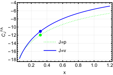
Figure 3: The same as Fig. 2, but for the profile of sub-coefficient $\mathcal{C}^{FA}_{J}(x)$ which has a pre-factor $C_{F}C_{A}$.

IV Numerical results and discussions

In the following, we will give the numerical results for the matching coefficients $\mathcal{C}_{J}(\mu_{f},\mu,m_{b},x)$ with $J=p,~{}v$ at NNLO accuracy. The sub-coefficients $\mathcal{C}^{FF}_{J}$, $\mathcal{C}^{FA}_{J}$, $\mathcal{C}^{FL}_{J}$, and $\mathcal{C}^{FH}_{J}$ classified by different color/flavor structures in Eq. (III) are functions which only depend on the heavy quark mass ratio with $x=\frac{m_{c}}{m_{b}}$. At physical heavy quark mass ratio, i.e., $x=x_{0}=\frac{1.5}{4.75}$ Qiao:2012hp ; Qiao:2012vt ; Qiao:2011zc , we obtained the following highly accurate numerical results with about 30-digit precision for all four kinds of sub-coefficients.

$$\mathcal{C}^{FF}_{p}(x_{0})=-18.1856109097151570253549607713,$$ (18)

$$\mathcal{C}^{FA}_{p}(x_{0})=-11.9709902751165587736864132992,$$ (19)

$$\mathcal{C}^{FL}_{p}(x_{0})=0.461971258745060837844427133019,$$ (20)

$$\mathcal{C}^{FH}_{p}(x_{0})=1.64553283592627680478382129760.$$ (21)

$$\mathcal{C}^{FF}_{v}(x_{0})=-15.8653228579431784031838005865,$$ (22)

$$\mathcal{C}^{FA}_{v}(x_{0})=-11.0678680506800630685188604612,$$ (23)

$$\mathcal{C}^{FL}_{v}(x_{0})=1.08196339731790945235792891668,$$ (24)

$$\mathcal{C}^{FH}_{v}(x_{0})=1.87201601140852309779426933441.$$ (25)

In order to investigate the heavy quark mass dependence of the matching coefficients, we vary the heavy quark mass ratio $x$ from $x_{min}=0.05$ to $x_{max}=1.2$. And we plotted the the heavy quark mass ratio $x$ dependence for the sub-coefficients $\mathcal{C}^{FF}_{J}$, $\mathcal{C}^{FA}_{J}$, $\mathcal{C}^{FL}_{J}$, and $\mathcal{C}^{FH}_{J}$ in Fig. 2, Fig. 3, Fig. 4, and Fig. 5, respectively. In these diagrams, $J=p$ represents the sub-coefficient for the pseudoscalar current while $J=v$ represents the sub-coefficient for the vector current. From the curves in Figs. (2-5), one can see the sub-coefficients are close to each other for both pseudoscalar and vector currents, except $\mathcal{C}^{FL}_{J}$. The sub-coefficients $\mathcal{C}^{FF}_{J}$ and $\mathcal{C}^{FA}_{J}$ increase gradually with the increase of the heavy quark mass ratio, while $\mathcal{C}^{FL}_{J}$ and $\mathcal{C}^{FH}_{J}$ first increase and then reduce with the increase of the heavy quark mass ratio.

Fixing the renormalization scale $\mu=m_{b}=4.75\mathrm{GeV}$, $m_{c}=1.5\mathrm{GeV}$, and setting the factorization scale $\mu_{f}=1.2\mathrm{GeV}$, Eq. (III) then reduces to

$$\mathcal{C}_{p}(\mu_{f}=1.2\mathrm{GeV},x=x_{0})=$$

$$1-1.40061\frac{\alpha_{s}^{(n_{l}=3)}(m_{b})}{\pi}-30.69707\left(\frac{\alpha_{s}^{(n_{l}=3)}(m_{b})}{\pi}\right)^{2}+\mathcal{O}(\alpha^{3}_{s}),$$ (26)

$$\mathcal{C}_{v}(\mu_{f}=1.2\mathrm{GeV},x=x_{0})=$$

$$1-2.06727\frac{\alpha_{s}^{(n_{l}=3)}(m_{b})}{\pi}-33.56657\left(\frac{\alpha_{s}^{(n_{l}=3)}(m_{b})}{\pi}\right)^{2}+\mathcal{O}(\alpha^{3}_{s}).$$ (27)

After obtaining the value of $\alpha_{s}^{(n_{l}=3)}$ by Eq. (11), we present our numerical results of the matching coefficients for the pseudoscalar current and the vector current in Fig. 6 and Fig. 7. From the figures, one can see the high-order corrections bring large scale-dependence in matching coefficients. This can be understood because the leading-order of matching coefficients is renormalized to 1. The scale-dependence in NLO corrections only rely on strong coupling constant at $\alpha_{s}(\mu)$. The scale-dependence in NNLO corrections not only rely on The strong coupling constant at $\alpha^{2}_{s}(\mu)$ but also the residue terms at order of $\alpha^{2}_{s}(\mu)\ln\mu^{2}$ which are not small for low scales. We summarize the results of the matching coefficients $\mathcal{C}_{J}$ for pseudoscalar and vector current decay constants at LO, NLO and NNLO accuracy in Tab. 1, where the uncertainties from all the parameters are included. From Tab. 1, the two largest uncertainties are from the factorization scale $\mu_{f}$ and the renormalization factor $\mu$ at NNLO, while the uncertainties from the bottom and charm quark are relatively small.

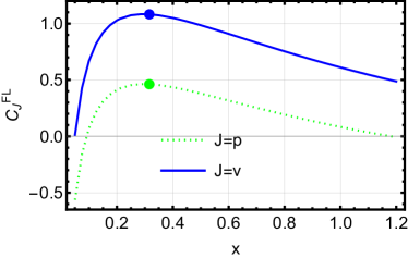
Figure 4: The same as Fig. 2, but for the profile of sub-coefficient $\mathcal{C}^{FL}_{J}(x)$ which has a pre-factor $C_{F}T_{F}n_{l}$.

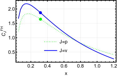
Figure 5: The same as Fig. 2, but for the profile of sub-coefficient $\mathcal{C}^{FH}_{J}(x)$ which has a pre-factor $C_{F}T_{F}$.

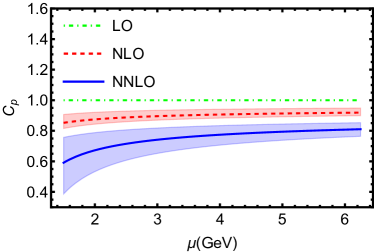
Figure 6: The renormalization scale dependence of the matching coefficient $\mathcal{C}_{p}$ for pseudoscalar current decay constant at LO, NLO and NNLO accuracy. The central values of the matching coefficient $\mathcal{C}_{p}$ are calculated inputting the physical values with $\mu_{f}=1.2\mathrm{GeV}$, $m_{b}=4.75\mathrm{GeV}$ and $m_{c}=1.5\mathrm{GeV}$. The error bands come from varying $\mu_{f}$ from 1.5 to 1 $\mathrm{GeV}$, $m_{b}$ from 5.25 to 4.25 $\mathrm{GeV}$, $m_{c}$ from 2 to 1 $\mathrm{GeV}$.

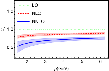
Figure 7: The same as Fig. 6, but for the matching coefficient $\mathcal{C}_{v}$ for vector current decay constant.

Table 1: The matching coefficients for both pseudoscalar and vector currents up to NNLO. The central values of the matching coefficient $\mathcal{C}_{J}$ are calculated inputting the physical values with $\mu_{f}=1.2\mathrm{GeV}$, $\mu=4.75\mathrm{GeV}$, $m_{b}=4.75\mathrm{GeV}$ and $m_{c}=1.5\mathrm{GeV}$. The errors are estimated by varying $\mu_{f}$ from 1.5 to 1 $\mathrm{GeV}$, $\mu$ from 6.25 to 3 $\mathrm{GeV}$, $m_{b}$ from 5.25 to 4.25 $\mathrm{GeV}$, and $m_{c}$ from 2 to 1 $\mathrm{GeV}$, respectively.

	LO	NLO	NNLO
$\mathcal{C}_{p}$	$1$	$0.9117^{-0+0.0072+0.0061-0.0156}_{+0-0.0160-0.0064+0.0263}$	$0.7897^{-0.0310+0.0206+0.0119+0.0149}_{+0.0253-0.0482-0.0133-0.0141}$
$\mathcal{C}_{v}$	$1$	$0.8697^{-0+0.0107+0.0061-0.0156}_{+0-0.0236-0.0064+0.0263}$	$0.7363^{-0.0234+0.0230+0.0106+0.0117}_{+0.0191-0.0526-0.0117-0.0121}$

Note that the explicit analytical expression for $\mathcal{C}_{a(\mu=0)}$ is given in Ref. Chen:2015csa at NNLO accuracy and the numerical results for $\mathcal{C}_{a(\mu=0)}$ is given in Ref. Feng:2022ruy at NNNLO accuracy. Our results are consistent with the previous results in Refs. Onishchenko:2003ui ; Chen:2015csa ; Feng:2022ruy . Even though the QCD theory makes the two decay constants from pseudoscalar current and axial current(timelike-component) identical, i.e. $\mathcal{C}_{p}=\mathcal{C}_{a(\mu=0)}$. Here we have explicit examined this point by the independent calculation of the pseudoscalar decay constants. On the other hand, the results for vector $B_{c}$ meson decay constant and its matching coefficient are novel. In the case of $m_{b}=m_{c}=m_{Q}$, our result for the vector current agrees with the previous results in literatures Kniehl:2006qw ; Egner:2022jot .

For the pseudoscalar meson $B_{c}$ and vector meson $B_{c}^{*}$, the leptonic decay widths can be written as

$$\Gamma(B^{+}_{c}\to l^{+}+{\nu}_{l})=\frac{{|V_{bc}|}^{2}}{8\pi}G_{F}^{2}m_{B_{c}}m_{l}^{2}\left(1-\frac{m_{l}^{2}}{m_{B_{c}}^{2}}\right)^{2}{f^{p}_{B_{c}}}^{2},$$ (28)

$$\Gamma(B_{c}^{*+}\to l^{+}+{\nu}_{l})=\frac{{|V_{bc}|}^{2}}{12\pi}G_{F}^{2}m_{B_{c}^{*}}^{3}\left(1-\frac{m_{l}^{2}}{m_{B_{c}^{*}}^{2}}\right)^{2}\left(1+\frac{m_{l}^{2}}{2m_{B_{c}^{*}}^{2}}\right){f^{v}_{B_{c}^{*}}}^{2}.$$ (29)

To evaluate the two decay constants $f^{p}_{B_{c}}$ and $f^{v}_{B^{*}_{c}}$, we substitute the LDMEs in Eq. (4) with

$$\left\langle 0\left|\chi^{\dagger}_{b}\mathbf{\sigma}\psi_{c}\right|B^{*}_{c}(\mathbf{P})\right\rangle\approx\left\langle 0\left|\chi^{\dagger}_{b}\psi_{c}\right|B_{c}(\mathbf{P})\right\rangle\approx\sqrt{2N_{c}}\;\psi_{B_{c}}(0),$$ (30)

where $\psi_{B_{c}}(0)$ is the Schrödinger wave function at the origin for $B_{c}$ system and is predicted in potential models Feng:2022ruy ; Eichten:1995ch ; Kiselev:2000jc ; Ikhdair:2003ry ; Shen:2021dat as

$$|\psi_{B_{c}}(0)|^{2}\simeq[0.10,0.13]\mathrm{GeV}^{3}.$$ (31)

The values of input parameters are extracted from the latest PDG group Workman:2022ynf as following:

$$V_{bc}=0.0408,~{}G_{F}=1.16638\times 10^{-5}\mathrm{GeV}^{-2},$$

$$m_{e}=0.000510999\mathrm{GeV},~{}m_{\mu}=0.10566\mathrm{GeV},$$

$$m_{\tau}=1.777\mathrm{GeV},~{}m_{B_{c}}=6.274\mathrm{GeV},~{}\tau_{B_{c}}=0.51\times 10^{-12}\mathrm{s}.$$

For $B^{*}_{c}$, there are many theoretical predictions for its mass and decay widths Godfrey:2004ya ; Wang:2022cxy ; Sun:2022hyk . We use the following values in Refs. Godfrey:2004ya ; Zhou:2017svh

$$m_{B_{c}^{*}}=6.314\mathrm{GeV},~{}~{}\Gamma_{\mathrm{tot}}(B_{c}^{*})=0.08\times 10^{-6}\mathrm{GeV}.$$

With the values of above input parameters, we present our predictions to $B_{c}$ and $B_{c}^{*}$ decay constants in Tab. 2.

Table 2: The predicted decay constants $f^{p}_{B_{c}}$ and $f^{v}_{B^{*}_{c}}$ up to NNLO. The central values are calculated inputting the physical values with $\psi_{B_{c}}(0)=\sqrt{0.12}\mathrm{GeV}^{\frac{3}{2}}$, $\mu_{f}=1.2\mathrm{GeV}$, $\mu=4.75\mathrm{GeV}$, $m_{b}=4.75\mathrm{GeV}$ and $m_{c}=1.5\mathrm{GeV}$. The errors are estimated by varying $\psi_{B_{c}}(0)$ from $\sqrt{0.13}$ to $\sqrt{0.10}$ $\mathrm{GeV}^{\frac{3}{2}}$, $\mu_{f}$ from 1.5 to 1 $\mathrm{GeV}$, $\mu$ from 6.25 to 3 $\mathrm{GeV}$, $m_{b}$ from 5.25 to 4.25 $\mathrm{GeV}$, and $m_{c}$ from 2 to 1 $\mathrm{GeV}$, respectively.

	$\frac{f^{p}_{B_{c}}}{10^{-1}\mathrm{GeV}}$	$\frac{f^{v}_{B^{*}_{c}}}{10^{-1}\mathrm{GeV}}$
LO	$4.79^{+0.20+0+0+0+0}_{-0.42-0-0-0-0}$	$4.78^{+0.20+0+0+0+0}_{-0.42-0-0-0-0}$
NLO	$4.37^{+0.18+0+0.03+0.03-0.07}_{-0.38-0-0.08-0.03+0.13}$	$4.15^{+0.17+0+0.05+0.03-0.07}_{-0.36-0-0.11-0.03+0.13}$
NNLO	$3.78^{+0.15-0.15+0.10+0.06+0.07}_{-0.33+0.12-0.23-0.06-0.07}$	$3.52^{+0.14-0.11+0.11+0.05+0.06}_{-0.31+0.09-0.25-0.06-0.06}$

Then we present our predictions to $B_{c}$ and $B_{c}^{*}$ leptonic decay widths in Tab. 3, Tab. 4, and Tab. 5, as well as the corresponding branching ratios in Tab. 6.

Table 3: The predicted leptonic decay width $\Gamma(B_{c}^{+}\to e^{+}+{\nu}_{e})$ and $\Gamma(B_{c}^{+*}\to e^{+}+{\nu}_{e})$ up to NNLO. The central values are calculated inputting the physical values with $|\psi_{B_{c}}(0)|^{2}=0.12\mathrm{GeV}^{3}$, $\mu_{f}=1.2\mathrm{GeV}$, $\mu=4.75\mathrm{GeV}$, $m_{b}=4.75\mathrm{GeV}$ and $m_{c}=1.5\mathrm{GeV}$. The errors are estimated by varying $|\psi_{B_{c}}(0)|^{2}$ from 0.13 to 0.10 $\mathrm{GeV}^{3}$, $\mu_{f}$ from 1.5 to 1 $\mathrm{GeV}$, $\mu$ from 6.25 to 3 $\mathrm{GeV}$, $m_{b}$ from 5.25 to 4.25 $\mathrm{GeV}$, and $m_{c}$ from 2 to 1 $\mathrm{GeV}$, respectively.

	$\frac{\Gamma(B^{+}_{c}\to e^{+}+{\nu}_{e})}{10^{-21}\mathrm{GeV}}$	$\frac{\Gamma(B_{c}^{*+}\to e^{+}+{\nu}_{e})}{10^{-13}\mathrm{GeV}}$
LO	$3.39^{+0.28+0+0+0+0}_{-0.56-0-0-0-0}$	$3.45^{+0.29+0+0+0+0}_{-0.57-0-0-0-0}$
NLO	$2.82^{+0.23+0+0.04+0.04-0.10}_{-0.47-0-0.10-0.04+0.16}$	$2.61^{+0.22+0+0.06+0.04-0.09}_{-0.43-0-0.14-0.04+0.16}$
NNLO	$2.11^{+0.18-0.16+0.11+0.06+0.08}_{-0.35+0.14-0.25-0.07-0.07}$	$1.87^{+0.16-0.12+0.12+0.05+0.06}_{-0.31+0.10-0.26-0.06-0.06}$

Table 4: The same as Tab. 3, but for $\Gamma(B_{c}^{+}\to\mu^{+}+{\nu}_{\mu})$ and $\Gamma(B_{c}^{*+}\to\mu^{+}+{\nu}_{\mu})$.

	$\frac{\Gamma(B_{c}\to\mu^{+}+{\nu}_{\mu})}{10^{-16}\mathrm{GeV}}$	$\frac{\Gamma(B_{c}^{*}\to\mu^{+}+{\nu}_{\mu})}{10^{-13}\mathrm{GeV}}$
LO	$1.45^{+0.12+0+0+0+0}_{-0.24-0-0-0-0}$	$3.45^{+0.29+0+0+0+0}_{-0.57-0-0-0-0}$
NLO	$1.20^{+0.10+0+0.02+0.02-0.04}_{-0.20-0-0.04-0.02+0.07}$	$2.61^{+0.22+0+0.06+0.04-0.09}_{-0.43-0-0.14-0.04+0.16}$
NNLO	$0.90^{+0.08-0.07+0.05+0.03+0.03}_{-0.15+0.06-0.11-0.03-0.03}$	$1.87^{+0.16-0.12+0.12+0.05+0.06}_{-0.31+0.10-0.26-0.06-0.06}$

Table 5: The same as Tab. 3, but for $\Gamma(B_{c}^{+}\to\tau^{+}+{\nu}_{\tau})$ and $\Gamma(B_{c}^{*+}\to\tau^{+}+{\nu}_{\tau})$.

	$\frac{\Gamma(B_{c}^{+}\to\tau^{+}+{\nu}_{\tau})}{10^{-14}\mathrm{GeV}}$	$\frac{\Gamma(B_{c}^{*+}\to\tau^{+}+{\nu}_{\tau})}{10^{-13}\mathrm{GeV}}$
LO	$3.47^{+0.29+0+0+0+0}_{-0.58-0-0-0-0}$	$3.04^{+0.25+0+0+0+0}_{-0.51-0-0-0-0}$
NLO	$2.88^{+0.24+0+0.05+0.04-0.10}_{-0.48-0-0.10-0.04+0.17}$	$2.30^{+0.19+0+0.06+0.03-0.08}_{-0.38-0-0.12-0.03+0.14}$
NNLO	$2.16^{+0.18-0.17+0.11+0.07+0.08}_{-0.36+0.14-0.26-0.07-0.08}$	$1.65^{+0.14-0.10+0.10+0.05+0.05}_{-0.27+0.09-0.23-0.05-0.05}$

Table 6: The predictions of leptonic branching ratios of $B_{c}$ and $B_{c}^{*}$ at NNLO. The central values are calculated inputting the physical values with $|\psi_{B_{c}}(0)|^{2}=0.12\mathrm{GeV}^{3}$, $\mu_{f}=1.2\mathrm{GeV}$, $\mu=4.75\mathrm{GeV}$, $m_{b}=4.75\mathrm{GeV}$ and $m_{c}=1.5\mathrm{GeV}$. The total errors come from varying $|\psi_{B_{c}}(0)|^{2}$ from 0.13 to 0.10 $\mathrm{GeV}^{3}$, $\mu_{f}$ from 1.5 to 1 $\mathrm{GeV}$, $\mu$ from 6.25 to 3 $\mathrm{GeV}$, $m_{b}$ from 5.25 to 4.25 $\mathrm{GeV}$, and $m_{c}$ from 2 to 1 $\mathrm{GeV}$.

	$e^{+}{\nu}_{e}$	$\mu^{+}{\nu}_{\mu}$	$\tau^{+}{\nu}_{\tau}$
$B_{c}$	$\left(1.64^{+0.44}_{-0.71}\right)\times 10^{-9}$	$\left(7.00^{+1.89}_{-3.01}\right)\times 10^{-5}$	$\left(1.68^{+0.45}_{-0.72}\right)\times 10^{-2}$
$B_{c}^{*}$	$\left(2.34^{+0.61}_{-1.01}\right)\times 10^{-6}$	$\left(2.34^{+0.61}_{-1.01}\right)\times 10^{-6}$	$\left(2.06^{+0.54}_{-0.89}\right)\times 10^{-6}$

From Tabs. 3, 4, and 5, the leptonic decay widths for $B^{*}_{c}$ are around $10^{-13}\mathrm{GeV}$, while the electronic, muonic and tauonic decay widths for $B_{c}$ are around $10^{-21}\mathrm{GeV}$, $10^{-16}\mathrm{GeV}$, $10^{-14}\mathrm{GeV}$, respectively. From Tab. 6, one can see the leptonic branching ratios for $B^{*}_{c}$ are around $10^{-6}$. The branching ratio for the tauonic decay of $B_{c}$ is around $10^{-2}$ while the branching ratio for the muonic decay of $B_{c}$ is around $10^{-4}-10^{-5}$ .

Consider the hadronic production of $B_{c}$ and $B^{*}_{c}$ has a large uncertainty and their cross-sections at LHC are from tens to hundreds nanobarn Chang:2003cq ; Chang:2003cr ; Chang:2005hq , there are tens to hundreds $B_{c}^{*+}\to l^{+}+{\nu}_{l}$ events, while hundreds to thousands $B_{c}^{+}\to\mu^{+}+{\nu}_{\mu}$ events at LHC for $1fb^{-1}$ proton proton collision data at 14TeV. Of course, the branching ratio of $B_{c}^{+}\to\tau^{+}+{\nu}_{\tau}$ is around 3 order of the branching ratio of $B_{c}^{+}\to\mu^{+}+{\nu}_{\mu}$, thus this channel shall be also a good detect channel of $B_{c}$ meson if the reconstruction of tauon lepton is well-controlled. In total, we expect these leptonic decay channels for both $B_{c}$ and $B^{*}_{c}$ can be accessible at LHC precision experiments.

V Conclusion

In this paper, we have performed a NNLO calculation of the decay constants of beauty-charmed meson $B_{c}$ and $B^{*}_{c}$. The NNLO result for vector current decay constant is novel. The updated leptonic decay branching ratios combined with the latest extraction of NRQCD LDMEs of $B_{c}$ meson shall be tested in future experiments. Through the careful studies of the decay constants of $B_{c}$ meson, one can expect that more and more decay channels of beauty-charmed mesons are accessible and their absolute branching ratios can be measured. The novel results of the anomalous dimension for the vector current in NRQCD shall provide more information on the renormalization properties of the NRQCD LDMEs. The NNLO matching coefficients are also helpful to investigate the behaviours when the doubly heavy quarks are in their threshold region.

Appendix

Allowing $n_{b}$ quarks with mass $m_{b}$, $n_{c}$ quarks with mass $m_{c}$ and $n_{l}$ massless quarks appearing in the quark loop, bottom quark on-shell wave function renormalization constant up to NNLO reads

$$Z_{2,b} =1+\frac{\alpha_{s}}{\pi}C_{F}\bigg{\{}-\frac{3}{4\epsilon}-\frac{3}{4}\ln\frac{\mu^{2}}{m_{b}^{2}}-1-\frac{\epsilon}{16}\left(6\ln^{2}\frac{\mu^{2}}{m_{b}^{2}}+16\ln\frac{\mu^{2}}{m_{b}^{2}}+\pi^{2}+32\right)$$

$$-\epsilon^{2}\bigg{[}\frac{1}{8}\ln^{3}\frac{\mu^{2}}{m_{b}^{2}}+\frac{1}{2}\ln^{2}\frac{\mu^{2}}{m_{b}^{2}}+\left(2+\frac{\pi^{2}}{16}\right)\ln\frac{\mu^{2}}{m_{b}^{2}}-\frac{\zeta_{3}}{4}+\frac{\pi^{2}}{12}+4\bigg{]}\bigg{\}}$$

$$+\frac{\alpha_{s}^{2}}{\pi^{2}}C_{F}\bigg{\{}C_{F}\bigg{[}\frac{9}{32\epsilon^{2}}+\frac{1}{192\epsilon}\left(108\ln\frac{\mu^{2}}{m_{b}^{2}}+153\right)+\frac{9}{16}\ln^{2}\frac{\mu^{2}}{m_{b}^{2}}+\frac{51}{32}\ln\frac{\mu^{2}}{m_{b}^{2}}+\pi^{2}\ln 2-\frac{3\zeta_{3}}{2}-\frac{49\pi^{2}}{64}+\frac{433}{128}\bigg{]}$$

$$+C_{A}\bigg{[}\frac{11}{32\epsilon^{2}}-\frac{127}{192\epsilon}-\frac{11}{32}\ln^{2}\frac{\mu^{2}}{m_{b}^{2}}-\frac{215}{96}\ln\frac{\mu^{2}}{m_{b}^{2}}-\frac{1}{2}\pi^{2}\ln 2+\frac{3\zeta_{3}}{4}+\frac{5\pi^{2}}{16}-\frac{1705}{384}\bigg{]}$$

$$+T_{F}n_{b}\bigg{[}\frac{1}{16\epsilon}\left(4\ln\frac{\mu^{2}}{m_{b}^{2}}+1\right)+\frac{3}{8}\ln^{2}\frac{\mu^{2}}{m_{b}^{2}}+\frac{11}{24}\ln\frac{\mu^{2}}{m_{b}^{2}}-\frac{5\pi^{2}}{16}+\frac{947}{288}\bigg{]}$$

$$+T_{F}n_{c}\bigg{[}\frac{1}{16\epsilon}\left(4\ln\frac{\mu^{2}}{m_{b}^{2}}-8\ln x+1\right)+\frac{\pi^{2}x^{4}}{4}-\frac{5\pi^{2}x^{3}}{8}+\frac{7x^{2}}{4}-\frac{3\pi^{2}x}{8}+\frac{3}{8}\ln^{2}\frac{\mu^{2}}{m_{b}^{2}}+\frac{11}{24}\ln\frac{\mu^{2}}{m_{b}^{2}}$$

$$+\ln(x)\ln\left(x+1\right)\left(-\frac{3x^{4}}{2}-\frac{5x^{3}}{4}-\frac{3x}{4}-\frac{1}{2}\right)+\text{Li}_{2}\left(x\right)\left(-\frac{3x^{4}}{2}+\frac{5x^{3}}{4}+\frac{3x}{4}-\frac{1}{2}\right)$$

$$+\ln^{2}\left(x\right)\left(\frac{3x^{4}}{2}+1\right)-\text{Li}_{2}\left(-x\right)\left(\frac{3x^{4}}{2}+\frac{5x^{3}}{4}+\frac{3x}{4}+\frac{1}{2}\right)$$

$$+\ln\left(x\right)\left(x^{2}-\ln\frac{\mu^{2}}{m_{b}^{2}}-\ln\left(1-x\right)\left(\frac{3x^{4}}{2}-\frac{5x^{3}}{4}-\frac{3x}{4}+\frac{1}{2}\right)+\frac{2}{3}\right)+\frac{5\pi^{2}}{48}+\frac{443}{288}\bigg{]}$$

$$+T_{F}n_{l}\bigg{[}\frac{-1}{8\epsilon^{2}}+\frac{11}{48\epsilon}+\frac{1}{8}\ln^{2}\frac{\mu^{2}}{m_{b}^{2}}+\frac{19}{24}\ln\frac{\mu^{2}}{m_{b}^{2}}+\frac{\pi^{2}}{12}+\frac{113}{96}\bigg{]}\bigg{\}}.$$ (32)

And allowing $n_{b}$ quarks with mass $m_{b}$, $n_{c}$ quarks with mass $m_{c}$ and $n_{l}$ massless quarks appearing in the quark loop, charm quark on-shell wave function renormalization constant up to NNLO can be obtained as

$$Z_{2,c}={Z_{2,b}}|_{\,m_{b}\rightarrow m_{c};\,x\rightarrow\frac{1}{x};\,n_{b}\leftrightarrow n_{c}}.$$ (33)

Allowing $n_{b}$ quarks with mass $m_{b}$, $n_{c}$ quarks with mass $m_{c}$ and $n_{l}$ massless quarks appearing in the quark loop, bottom quark on-shell mass renormalization constant up to NNLO reads

$$Z_{m,b} =1+\frac{\alpha_{s}}{\pi}C_{F}\bigg{\{}-\frac{3}{4\epsilon}-\frac{3}{4}\ln\frac{\mu^{2}}{m_{b}^{2}}-1-\frac{\epsilon}{16}\left(6\ln^{2}\frac{\mu^{2}}{m_{b}^{2}}+16\ln\frac{\mu^{2}}{m_{b}^{2}}+\pi^{2}+32\right)$$

$$-\epsilon^{2}\bigg{[}\frac{1}{8}\ln^{3}\frac{\mu^{2}}{m_{b}^{2}}+\frac{1}{2}\ln^{2}\frac{\mu^{2}}{m_{b}^{2}}+\left(2+\frac{\pi^{2}}{16}\right)\ln\frac{\mu^{2}}{m_{b}^{2}}-\frac{\zeta_{3}}{4}+\frac{\pi^{2}}{12}+4\bigg{]}\bigg{\}}$$

$$+\frac{\alpha_{s}^{2}}{\pi^{2}}C_{F}\bigg{\{}C_{F}\bigg{[}\frac{9}{32\epsilon^{2}}+\frac{1}{192\epsilon}\left(108\ln\frac{\mu^{2}}{m_{b}^{2}}+135\right)+\frac{9}{16}\ln^{2}\frac{\mu^{2}}{m_{b}^{2}}+\frac{45}{32}\ln\frac{\mu^{2}}{m_{b}^{2}}+\frac{1}{2}\pi^{2}\ln 2-\frac{3\zeta_{3}}{4}-\frac{17\pi^{2}}{64}+\frac{199}{128}\bigg{]}$$

$$+C_{A}\bigg{[}\frac{11}{32\epsilon^{2}}-\frac{97}{192\epsilon}-\frac{11}{32}\ln^{2}\frac{\mu^{2}}{m_{b}^{2}}-\frac{185}{96}\ln\frac{\mu^{2}}{m_{b}^{2}}-\frac{1}{4}\pi^{2}\ln 2+\frac{3\zeta_{3}}{8}+\frac{\pi^{2}}{12}-\frac{1111}{384}\bigg{]}$$

$$+T_{F}n_{b}\bigg{[}\frac{-1}{8\epsilon^{2}}+\frac{5}{48\epsilon}+\frac{1}{8}\ln^{2}\frac{\mu^{2}}{m_{b}^{2}}+\frac{13}{24}\ln\frac{\mu^{2}}{m_{b}^{2}}-\frac{\pi^{2}}{6}+\frac{143}{96}\bigg{]}$$

$$+T_{F}n_{c}\bigg{[}\frac{-1}{8\epsilon^{2}}+\frac{5}{48\epsilon}+\frac{x^{4}}{2}\ln^{2}x+\frac{\pi^{2}x^{4}}{12}-\frac{\pi^{2}x^{3}}{4}+\frac{3x^{2}}{4}-\frac{\pi^{2}x}{4}+\frac{1}{8}\ln^{2}\frac{\mu^{2}}{m_{b}^{2}}+\frac{13}{24}\ln\frac{\mu^{2}}{m_{b}^{2}}$$

$$+\ln\left(x\right)\ln\left(x+1\right)\left(-\frac{x^{4}}{2}-\frac{x^{3}}{2}-\frac{x}{2}-\frac{1}{2}\right)+\text{Li}_{2}\left(x\right)\left(-\frac{x^{4}}{2}+\frac{x^{3}}{2}+\frac{x}{2}-\frac{1}{2}\right)$$

$$-\text{Li}_{2}\left(-x\right)\left(\frac{x^{4}}{2}+\frac{x^{3}}{2}+\frac{x}{2}+\frac{1}{2}\right)+\ln\left(x\right)\left(\frac{x^{2}}{2}-\ln\left(1-x\right)\left(\frac{x^{4}}{2}-\frac{x^{3}}{2}-\frac{x}{2}+\frac{1}{2}\right)\right)+\frac{\pi^{2}}{12}+\frac{71}{96}\bigg{]}$$

$$+T_{F}n_{l}\bigg{[}\frac{-1}{8\epsilon^{2}}+\frac{5}{48\epsilon}+\frac{1}{8}\ln^{2}\frac{\mu^{2}}{m_{b}^{2}}+\frac{13}{24}\ln\frac{\mu^{2}}{m_{b}^{2}}+\frac{\pi^{2}}{12}+\frac{71}{96}\bigg{]}\bigg{\}}.$$ (34)

And allowing $n_{b}$ quarks with mass $m_{b}$, $n_{c}$ quarks with mass $m_{c}$ and $n_{l}$ massless quarks appearing in the quark loop, charm quark on-shell mass renormalization constant up to NNLO can be obtained as

$$Z_{m,c}={Z_{m,b}}|_{\,m_{b}\rightarrow m_{c};\,x\rightarrow\frac{1}{x};\,n_{b}\leftrightarrow n_{c}}$$ (35)

References

- (1) F. Abe et al. (CDF Collaboration), Phys. Rev. Lett. 81, 2432-2437 (1998).
- (2) G. Aad et al. (ATLAS Collaboration), Phys. Rev. Lett. 113, 212004 (2014).
- (3) A. M. Sirunyan et al. (CMS Collaboration), Phys. Rev. Lett. 122, 132001 (2019).
- (4) R. Aaij et al. (LHCb Collaboration ), Phys. Rev. Lett. 122, 232001 (2019).
- (5) R. L. Workman et al. ( Particle Data Group), PTEP 2022, 083C01 (2022).
- (6) D. Becirevic et al. [ETM], PoS LATTICE2018, 273 (2019).
- (7) B. Colquhoun et al. [HPQCD], Phys. Rev. D 91, no.11, 114509 (2015).
- (8) J. Harrison et al. (HPQCD Collaboration ), Phys. Rev. D 102, 094518 (2020).
- (9) G. T. Bodwin, E. Braaten and G. P. Lepage, Phys. Rev. D 51, 1125-1171 (1995), [erratum: Phys. Rev. D 55, 5853 (1997)].
- (10) E. Braaten and S. Fleming, Phys. Rev. D 52, 181-185 (1995).
- (11) C. H. Chang and Y. Q. Chen, Phys. Rev. D 49, 3399-3411 (1994).
- (12) J. Lee, W. Sang and S. Kim, JHEP 01, 113 (2011).
- (13) A. I. Onishchenko and O. L. Veretin, Eur. Phys. J. C 50, 801-808 (2007).
- (14) L. B. Chen and C. F. Qiao, Phys. Lett. B 748, 443-450 (2015).
- (15) F. Feng, Y. Jia, Z. Mo, J. Pan, W. L. Sang and J. Y. Zhang, arXiv:2208.04302 [hep-ph].
- (16) P. Marquard, J. H. Piclum, D. Seidel and M. Steinhauser, Nucl. Phys. B 758, 144-160 (2006).
- (17) M. Egner, M. Fael, J. Piclum, K. Schoenwald and M. Steinhauser, Phys. Rev. D 104, 054033 (2021).
- (18) M. Beneke, A. Signer and V. A. Smirnov, Phys. Rev. Lett. 80, 2535-2538 (1998).
- (19) P. Marquard, J. H. Piclum, D. Seidel and M. Steinhauser, Phys. Lett. B 678, 269-275 (2009).
- (20) P. Marquard, J. H. Piclum, D. Seidel and M. Steinhauser, Phys. Rev. D 89, 034027 (2014).
- (21) B. A. Kniehl, A. A. Penin, M. Steinhauser and V. A. Smirnov, Phys. Rev. Lett. 90, 212001 (2003), [erratum: Phys. Rev. Lett. 91, 139903 (2003)].
- (22) M. Egner, M. Fael, F. Lange, K. Schönwald and M. Steinhauser, Phys. Rev. D 105, 114007 (2022).
- (23) W. L. Sang, F. Feng, Y. Jia, Z. Mo and J. Y. Zhang, arXiv: 2202.11615 [hep-ph].
- (24) F. Feng, Y. Jia, Z. Mo, J. Pan, W. L. Sang and J. Y. Zhang, arXiv:2207.14259 [hep-ph].
- (25) X. Chen, X. Guan, C. Q. He, X. Liu and Y. Q. Ma, arXiv:2209.14259 [hep-ph].
- (26) L. B. Chen, J. Jiang and C. F. Qiao, JHEP 04, 080 (2018).
- (27) W. Tao, Z. J. Xiao and R. Zhu, Phys. Rev. D 105, 114026 (2022).
- (28) R. Y. Tang, Z. R. Huang, C. D. Lü and R. Zhu, J. Phys. G 49, 115003 (2022).
- (29) R. Zhu, Nucl. Phys. B 931, 359-382 (2018).
- (30) R. Zhu, Y. Ma, X. L. Han and Z. J. Xiao, Phys. Rev. D 95, 094012 (2017).
- (31) J. Zhao and P. Zhuang, arXiv:2209.13475 [hep-ph].
- (32) M. Bordone, A. Khodjamirian and T. Mannel, arXiv: 2209. 08851 [hep-ph].
- (33) C. Sun, R. H. Ni and M. Chen, arXiv:2209.06724 [hep-ph].
- (34) Z. J. Xiao and X. Liu, Chin. Sci. Bull. 59, 3748-3759 (2014).
- (35) Z. G. Wang, Eur. Phys. J. A 49, 131 (2013).
- (36) J. H. Piclum, doi:10.3204/DESY-THESIS-2007-014.
- (37) V. Shtabovenko, R. Mertig and F. Orellana, Comput. Phys. Commun. 256, 107478 (2020).
- (38) F. Feng, Comput. Phys. Commun. 183, 2158-2164 (2012).
- (39) J. Klappert, F. Lange, P. Maierhöfer and J. Usovitsch, Comput. Phys. Commun. 266, 108024 (2021).
- (40) A. V. Smirnov and F. S. Chuharev, Comput. Phys. Commun. 247, 106877 (2020).
- (41) T. Peraro, JHEP 07, 031 (2019).
- (42) K. G. Chetyrkin and F. V. Tkachov, Nucl. Phys. B 192, 159-204 (1981).
- (43) X. Liu and Y. Q. Ma, arXiv:2201.11669 [hep-ph].
- (44) X. Liu, Y. Q. Ma and C. Y. Wang, Phys. Lett. B 779, 353-357 (2018).
- (45) B. A. Kniehl, A. Onishchenko, J. H. Piclum and M. Steinhauser, Phys. Lett. B 638, 209-213 (2006).
- (46) R. Bonciani and A. Ferroglia, JHEP 11, 065 (2008).
- (47) A. I. Davydychev, P. Osland and O. V. Tarasov, Phys. Rev. D 58, 036007 (1998).
- (48) T. de Oliveira, D. Harnett, A. Palameta and T. G. Steele, arXiv:2208.12363 [hep-ph].
- (49) S. Bekavac, A. Grozin, D. Seidel and M. Steinhauser, JHEP 10, 006 (2007).
- (50) M. Fael, K. Schönwald and M. Steinhauser, JHEP 10, 087 (2020).
- (51) K. G. Chetyrkin, J. H. Kuhn and C. Sturm, Nucl. Phys. B 744, 121-135 (2006).
- (52) W. Bernreuther and W. Wetzel, Nucl. Phys. B 197, 228-236 (1982), [erratum: Nucl. Phys. B 513, 758-758 (1998)].
- (53) P. Bärnreuther, M. Czakon and P. Fiedler, JHEP 02, 078 (2014).
- (54) A. G. Grozin, P. Marquard, J. H. Piclum and M. Steinhauser, Nucl. Phys. B 789, 277-293 (2008).
- (55) M. A. Özcelik, tel-03362708.
- (56) K. G. Chetyrkin, B. A. Kniehl and M. Steinhauser, Phys. Rev. Lett. 79, 2184-2187 (1997).
- (57) K. G. Chetyrkin, J. H. Kuhn and M. Steinhauser, Comput. Phys. Commun. 133, 43-65 (2000).
- (58) A. Deur, S. J. Brodsky and G. F. de Teramond, Nucl. Phys. 90, 1 (2016).
- (59) F. Herren and M. Steinhauser, Comput. Phys. Commun. 224, 333-345 (2018).
- (60) C. F. Qiao, P. Sun, D. Yang and R. L. Zhu, Phys. Rev. D 89, 034008 (2014).
- (61) C. F. Qiao and R. L. Zhu, Phys. Rev. D 87, 014009 (2013).
- (62) C. F. Qiao, L. P. Sun and R. L. Zhu, JHEP 08, 131 (2011).
- (63) E. J. Eichten and C. Quigg, Phys. Rev. D 52, 1726-1728 (1995).
- (64) V. V. Kiselev, A. E. Kovalsky and A. I. Onishchenko, Phys. Rev. D 64, 054009 (2001) doi:10.1103/PhysRevD.64.054009 [arXiv:hep-ph/0005020 [hep-ph]].
- (65) S. M. Ikhdair and R. Sever, Int. J. Mod. Phys. A 19, 1771-1792 (2004).
- (66) D. Shen, H. Ren, F. Wu and R. Zhu, Int. J. Mod. Phys. A 36, 2150135 (2021).
- (67) S. Godfrey, Phys. Rev. D 70, 054017 (2004).
- (68) G. L. Wang, T. Wang, Q. Li and C. H. Chang, JHEP 05, 006 (2022).
- (69) B. B. Zhou, J. J. Sun and Y. J. Zhang, Commun. Theor. Phys. 67, 655 (2017).
- (70) C. H. Chang, C. Driouichi, P. Eerola and X. G. Wu, Comput. Phys. Commun. 159, 192-224 (2004).
- (71) C. H. Chang and X. G. Wu, Eur. Phys. J. C 38, 267-276 (2004).
- (72) C. H. Chang, J. X. Wang and X. G. Wu, Comput. Phys. Commun. 174, 241-251 (2006).