Kaluza-Klein theory for type $II\ b$ supergravity on the warped deformed conifold

Abstract

We discuss Kaluza-Klein theory for type $II\ b$ supergravity on the warped deformed conifold using a large radial distance limit of Klebanov-Strassler solution where the radial coordinate separates from angle coordinates for a background asymptotic to $AdS_{5}\times T^{1,1}$ spacetime. The decomposition of field fluctuations on harmonics of the base manifold $T^{1,1}$ and plane waves of $M_{4}=\partial(AdS_{5})$ is examined for the metric tensor components along $M_{4}=\partial(AdS_{5})$, the axio-dilaton and the 4-form potential components along $T^{1,1}$. Semi-classical methods are used to compute the mass spectra, wave functions and interactions for a set of modes in low dimensional representations of the isometry group. Deformations of the background solution due to compactification effects are also considered. The information on warped modes properties is utilized to explore the thermal evolution of a cosmic component of metastable modes after exit from brane inflation.

I Introduction

The discussion of string theory flux compactifications dougkach05 ; granarev05 in the context of gauge-string duality malda99 has opened novel perspectives to particle physics models invoking warped extra space dimensions rs9905 ; rs9906 . The attractive synthesis of proposals to anchor the models in string theory becker96 ; acharya99 ; verlinde99 ; dasgupta99 ; becker00 ; greene00 ; becker01 , realized through the Giddings, Kachru and Polchinski (GKP) gkp01 construction of type $II\ b$ superstring theory compactifications, has led to progress on both formal dealvisflux03 ; gidd05 ; firouz06 ; dougba07 ; dougtorr08 ; shiu08 ; frey08 ; douglas09 ; freyroberts13 and phenomenological kofman05 ; chen06 ; berndsen07 ; kofman08 ; freydacline09 ; chemtob16 grounds.

Pursuing along these lines, we examine in this work the Kaluza-Klein theory for 10-d supergravity theory reduced on a warped deformed conifold throat candelas90 glued to a conic Calabi-Yau orientifold $X_{6}$. To ease computations, we consider replacing the spacetime metric in Klebanov-Strassler solution klebstrass00 by an approximate factorizable ansatz. Instead of modifying the deformed conifold ${\cal C}_{6}$ radial section to copies of a sub-manifold of $S^{3}\times S^{2}$ geometry, as proposed in firouz06 , we consider a large radial distance limit where the conifold radial coordinate $\tau$ separates from the angular coordinates $\Theta_{\alpha},\ [a=1,\cdots,5]$ of the sub-manifold $T^{1,1}$ leading to a geometry asymptotic to $AdS_{5}\times T^{1,1}$ spacetime. The dimensional reduction can then be performed along standard lines kiroman84 ; ceresole99 ; ceresoII99 , easing the comparison with the dual Klebanov-Witten gauge theory klewit98 .

The decomposition of supergravity multiplet fields on harmonic functions of $T^{1,1}$ yields a field theory in Minkowski spacetime $M_{4}=\partial(AdS_{5})$ with towers of modes whose masses and radial wave functions satisfy a Sturm-Liouville boundary eigenvalue problem. We derive the wave equations for warped modes descending from the metric tensor field along $M_{4}$, the 4-form potential field along $T^{1,1}$ and the axio-dilaton field and compute their properties (mass spectra, wave functions and local couplings). We present results in the throat domination regime ignoring the throat-bulk interface and selecting normalizable modes along the conifold radial direction. The semi-classical WKB (Wentzel-Kramers-Brillouin) method is applied to obtain the wave functions and mass parameters for a set of singlet and charged modes under the conifold isometry group with the view to identify candidates for the lightest charged Kaluza-Klein particle (LCKP). We also obtain predictions for the cubic and higher order self couplings of bulk modes and for their couplings to $D3$-branes embedded near the conifold apex.

The information on warped modes motivates us to examine their cosmological impact on the universe reheating in the $(D-\bar{D})$-brane inflation scenario kklt03 ; kklmmt03 ; baumann06 ; baumann08 . We examine the possibility that the interacting gas of Kaluza-Klein particles produced in the inflationary throat could reach thermal equilibrium before decaying or could tunnel out to a neighboring throat hosting Standard Model branes barnaby04 ; frey05 ; chialva05 ; kofman05 ; chen06 ; kofman08 ; chialva12 . We also explore in these two cases the possibility that a fraction of metastable modes might survive as a cold thermal relic that could decay at later times berndsen07 ; freydacline09 ; chen09 .

The contents of this work are organized into four sections. In Section II, we review the constuction of GKP flux vacua of type $II\ b$ supergravity on the spacetime $M_{4}\times X_{6}$ with an attached deformed conifold throat described by Klebanov-Strassler solution. In Section III, we examine the Kaluza-Klein reduction of bosonic field components of the supergravity multiplet at large radial distances inside ${\cal C}_{6}$ where the background warped asymptotes $AdS_{5}\times T^{1,1}$ spacetime. The harmonic decomposition of fields is applied in Subsections III.1 and III.2 to derive the wave equations for fluctuations of the (unwarped) metric tensor $\tilde{g}_{\mu\nu}$ along $M_{4}$, the real scalar from the 4-form potential $C_{abcd}(X)$ along $T^{1,1}$ and the axio-dilaton $\tau(X)$. Numerical results are presented in Subsection III.3 for the mass spectra and wave functions of a selected set of warped modes in low dimensional representations of the conifold isometry group.

The central issue in this work concerning warped modes interactions is discussed in Section IV. Subsection IV.1 deals with the mutual couplings of graviton modes, Subsection IV.2 with compactification effects on warped modes couplings using the perturbative AdS/CFT duality approach of gandhi11 and Subsection IV.3 with trilinear couplings between graviton and scalar modes. In Section V we consider a cosmic population of warped modes produced after brane inflation and examine both its thermal evolution and ability to leave a cold thermal relic. Subsection V.1 discusses general assumptions, Subsection V.2 a single throat scenario and Subsection V.3 a double throat scenario. In Section VI we present main conclusions. An introductory review of the deformed conifold is presented in Appendix A. Subsection A.1 discusses the algebraic properties, Subsection A.2 the harmonic analysis pufu10 , Subsection A.3 the approximate separable version of Klebanov-Strassler metric involving a cone over a base manifold of geometry $S^{2}\times S^{3}$ firouz06 and Subsection A.4 the approximate analytic formalism bridging between the deformed and undeformed conifold cases.

II Type $II\ b$ supergravity theory on the conifold

II.1 Warped background spacetime for 10-d supergravity

Our discussions will mostly concentrate on the classical bosonic action of 10-d type $II\ b$ supergravity theory in Einstein frame,

$$S_{IIb}={m_{D}^{8}\over 2}\int d^{10}X\bigg{[}\sqrt{-g}\bigg{(}R-{|\partial_{M}\tau|^{2}\over 2\tau_{2}^{2}}-{1\over 2\tau_{2}}G_{3}\cdot\bar{G}_{3}-{1\over 4}\tilde{F}_{5}\cdot\tilde{F}_{5}\bigg{)}-{i\over 4\tau_{2}}C_{4}\wedge G_{3}\wedge\bar{G}_{3}\bigg{]}$$ (II.1)

$$={2\pi\over\hat{l}_{s}^{8}}\int d^{10}X\bigg{[}\sqrt{-g}\bigg{(}R-{1\over 2}((\partial_{M}\phi)^{2}+e^{2\phi}(\partial_{M}C_{0})^{2})-{1\over 2}(e^{-\phi}|H_{3}|^{2}+e^{\phi}|\tilde{F}_{3}|^{2})-{1\over 4}|\tilde{F}_{5}|^{2}\bigg{)}-{1\over 4}C_{4}\wedge\tilde{F}_{3}\wedge H_{3}\bigg{]},$$ (II.2)

$$[F_{1}=dC_{0},\ F_{3}=dC_{2},\ F_{5}=dC_{5},\ \tilde{F}_{3}=F_{3}-C_{0}\wedge H_{3},$$ (II.3)

$$\tilde{F}_{5}=\star_{10}\tilde{F}_{5}=F_{5}-{1\over 2}C_{2}\wedge H_{3}+{1\over 2}B_{2}\wedge F_{3},\ \tau\equiv\tau_{1}+i\tau_{2}=C_{0}+ie^{-\phi},\ G_{3}=F_{3}-\tau H_{3}=\tilde{F}_{3}-ie^{-\phi}H_{3}]$$ (II.4)

where the action is derived from the string frame action via the metric tensor rescaling, $g^{s}_{MN}\to e^{\phi/2}g_{MN}$. The gravitational mass scale ${2/m_{D}^{8}}=2\kappa^{2}_{10}={(2\pi)^{7}}\alpha^{{}^{\prime}4}={\hat{l}_{s}^{8}/(2\pi)},\ [\hat{l}_{s}=2\pi l_{s}]$ is set by the string inverse tension $\alpha^{\prime}=1/m_{s}^{2}$, independently of the string coupling constant $g_{s}=<e^{\phi}>$. Our notational conventions and system of units, $\hbar=c=1$, are same as in our earlier work chemtob16 which specialized, however, to the alternative Einstein frame derived from the string frame by the replacement $ds^{2}_{10}\to(e^{\phi}/g_{s})^{1/2}ds^{2}_{10}$, changing the gravitational mass scale $\kappa^{2}_{10}\to\kappa^{2}=g_{s}^{2}\kappa^{2}_{10}.$

The classical vacua for background spacetimes $M_{4}\times X_{6}$ preserving ${\cal N}=1$ supersymmetry involve conic Calabi-Yau orientifolds $X_{6}$ with 3-fluxes $\int_{A}F_{3}=\hat{l}_{s}^{2}M,\ \int_{B}H_{3}=-\hat{l}_{s}^{2}K$ across dual 3-cycles $A,\ B$ sourcing a warped spacetime region near the conifold singularity of $X_{6}$. The background may also include spacetime filling $O3/O7$-planes and probe $D3/D7$-branes that carry effective $D3$-brane charges $N_{O3},\ N_{D3}$ satisfying the $C_{4}$-tadpole cancellation condition, $MK+N_{D3}-{1\over 4}N_{O3}=0$. We consider the family of GKP classical solutions gkp01 involving an imaginary self dual 3-form field strength, $G_{-}\equiv(\star_{6}-i)G_{3}=0$, a constant axio-dilaton, $\tau(y)={i/g_{s}}$, metric tensor and 5-form field strength of form,

$$ds^{2}_{10}=ds^{2}_{4}+ds^{2}_{6}=e^{2A(y)}d\tilde{s}^{2}_{4}+e^{-2A(y)}d\tilde{s}^{2}_{6},\ F_{5}=(1+\star_{10})d\alpha(y)\wedge vol(M_{4}),$$ (II.5)

$$[h^{-1}(y)=e^{4A(y)}=\alpha(y),\ d\tilde{s}^{2}_{4}=\tilde{g}_{\mu\nu}dx^{\mu}dx^{\nu},\ d\tilde{s}^{2}_{6}=\tilde{g}_{mn}dy^{m}dy^{n}]$$ (II.6)

along with localized sources whose stress energy-momentum tensor $T_{MN}^{loc}$ and effective $D3$-brane charge density $\rho_{3}^{loc}$ satisfy the BPS-like inequality

$$\hat{T}^{loc}(y)-\tau_{3}\rho_{3}^{loc}(y)\geq 0,\ [\hat{T}^{loc}(y)={(T^{m}_{m}-T_{\mu}^{\mu})^{loc}\over 4},\ \tau_{p}={2\pi\over\hat{l}_{s}^{p+1}}].$$ (II.7)

(In the dual gauge theory description, the 3-fluxes $M,\ K$ and the induced 5-flux $N=MK$ dissolve into regular and fractional $N\ D3+M\ D5$-brane stacks.) One can relate the 4-d (Planck) gravitational mass scale, $\kappa^{-1}_{4}=M_{\star}=M_{P}/\sqrt{8\pi}\simeq 2.43\ 10^{18}$ GeV, to the supergravity mass scale, $\kappa^{2}_{10}=(2\pi)^{7}\alpha^{{}^{\prime}4}/2$, by matching the 10-d curvature action reduced on $X_{6}$ to the standard (Einstein-Hilbert) 4-d curvature action,

$${1\over 2\kappa^{2}_{10}}\int d^{10}X\sqrt{-g_{10}}R^{(10)}\simeq{1\over 2\kappa_{4}^{2}}\int d^{4}x\sqrt{-\tilde{g}_{4}}g^{\mu\nu}R^{(4)}_{\mu\nu}\ \Longrightarrow\ \kappa^{2}_{10}=\kappa_{4}^{2}V_{W}\equiv{V_{W}\over M_{\star}^{2}},\ [V_{W}=\int d^{6}y\sqrt{\tilde{g}}e^{-4A(y)}].$$ (II.8)

The resulting relation between gravitational scales, involving the 6-d internal manifold warped volume $V_{W}=(2\pi L_{W})^{6}$, with $L_{W}$ interpreted as the effective compactification radius, can be used to trade the string scale for the reduced Planck scale, $m_{s}=({\pi M_{\star}^{2}/L_{W}^{6}})^{1/8}$. Recall that warped compactifications exhibit a redundancy gkp01 ; gidd05 under rescalings of the warp profile and internal manifold $X_{6}$ unwarped metric, $e^{2A}\to\lambda e^{2A},\ \tilde{g}_{mn}\to\lambda\tilde{g}_{mn},\ [\lambda\in R_{+}]$ leaving the 10-d metric unchanged, $ds^{2}_{10}\to ds^{2}_{10}=\lambda e^{2A(y)}\tilde{g}_{\mu\nu}(x)dx^{\mu}dx^{\nu}+e^{-2A(y)}\tilde{g}_{mn}(y)dy^{m}dy^{n},$ up to the Weyl rescaling of the non-compact spacetime $M_{4}$ metric, $g_{\mu\nu}\to\lambda g_{\mu\nu}$. For a given internal manifold $X_{6}$ of warped metric $g_{mn}$, the classical background can then be described by a one-parameter family of solutions with warp profiles and unwarped internal space metric rescaled by the parameter $\lambda$. This establishes an equivalence between descriptions (frames) differing in the 4-d gravitational mass scale definition gidd05 ; shiu08 . The frame arbitrariness is neatly delineated by defining equivalence classes of 10-d frames, with respect to reference (fiducial) warp profile $A_{0}(y)$, 6-d manifold of metric $\tilde{g}^{0}_{mn}$ and volume $V^{0}=\int d^{6}y\sqrt{\tilde{g}^{0}_{6}}$ (carrying suffix label $0$), with parameter dependent metric and 4-d gravitational scale,

$$ds^{2}_{10}=\lambda e^{2A_{0}(y)}\tilde{g}_{\mu\nu}(x)dx^{\mu}dx^{\nu}+e^{-2A_{0}(y)}\tilde{g}^{0}_{mn}(y)dy^{m}dy^{n},\ {1\over\kappa_{4}^{2}(\lambda)}={\lambda V_{W}^{0}\over\kappa_{10}^{2}},\ [V^{0}_{W}=\int d^{6}y\sqrt{\tilde{g}^{0}_{6}}e^{-4A_{0}}].$$ (II.9)

For the 10-d Einstein frame choice, $\lambda=V^{0}/V^{0}_{W}$, one finds ${1/\kappa_{4}^{2}}={V^{0}/\kappa_{10}^{2}}$ and for the 4-d Einstein frame choice $\lambda=1$, the result ${1/\kappa_{4}^{2}}={V^{0}_{W}/\kappa_{10}^{2}}$ reproduces the above matching relation, $V^{0}_{W}=V_{W}$. (Going from the 4-d to 10-d Einstein frames replaces the 4-d metric and gravitational scale as, $g_{\mu\nu}\to(V^{0}/V_{W}^{0})g_{\mu\nu},\ {1/\kappa_{4}^{2}}\to(V^{0}/V_{W}^{0})/\kappa_{4}^{2}.$) A similar situation holds if one incorporates the universal volume modulus $c(x)$ through the $x$-dependent warp function $A(x,y)$ and define the family of 10-d metrics with respect the fiducial warp profile and 6-d metric $A_{0}(y)$ and $\tilde{g}^{0}_{mn}$ as gidd05

$$ds^{2}_{10}=\lambda e^{2A(x,y)}\tilde{g}_{\mu\nu}dx^{\mu}dx^{\nu}+e^{-2A(x,y)}\tilde{g}^{0}_{mn}dy^{m}dy^{n},\ [e^{-4A(x,y)}=c(x)+e^{-4A_{0}(y)}].$$ (II.10)

The equivalence under the metric and gravitational scale rescaling is then described by

$$e^{2A(x,y)}\to\lambda e^{2A(x,y)},\ \tilde{g}^{0}_{mn}\to\lambda\tilde{g}^{0}_{mn},\ {1\over\kappa_{4}^{2}(\lambda)}={\lambda V_{W}^{c}\over\kappa_{10}^{2}},\ [V_{W}^{c}=\int d^{6}y\sqrt{\tilde{g}^{0}_{mn}}e^{-4A(x,y)}=c(x)V^{0}+V_{W}^{0}]$$ (II.11)

with the 10-d Einstein frame defined by $\lambda=V^{0}/V_{W}^{c}$ and ${1/\kappa_{4}^{2}}=V^{0}/\kappa_{10}^{2}$ and the 4-d Einstein frame by $\lambda=1$ and ${1/\kappa_{4}^{2}}=V^{c}_{W}/\kappa_{10}^{2}$. (Going from the 10-d to 4-d Einstein frames multiplies $g_{\mu\nu}$ and ${1/\kappa_{4}^{2}}$ by $(V^{c}_{W}/V^{0}).$) We note incidentally that the non-trivial result frey08 for the Kähler potential of the chiral superfield $\rho(x)=ic(x)+a_{0}(x)$, comprising the universal volume modulus and axion field from the 4-form potential,

$$\kappa_{4}^{2}K(\rho,\ \bar{\rho})=-3\ln(2c(x)+2V_{W}^{0}/V^{0})=-3\ln(-i(\rho-\bar{\rho})+2V_{W}^{0}/V^{0}),$$ (II.12)

is reproduced here by the intuitive construct, $\kappa_{4}^{2}K=-3\ln(2V_{W}^{c}/V^{0}).$ In the large volume (dilute flux) limit, $c>>V_{W}^{0}/V^{0}$, the additive type volume modulus $c(x)$ is related as $c(x)=e^{4u(x)}$ to the multiplicative type modulus $u(x)$, which is introduced via the metric and 4-form fields rescaling, $g^{0}_{mn}\to e^{2u(x)}g^{0}_{mn},\ g_{\mu\nu}\to e^{-6u(x)}g_{\mu\nu},\ \alpha(y)\to e^{-12u(x)}\alpha(y)$. The (Einstein frame) Kähler potential is then expressed as $\kappa^{2}_{4}K(u)=-2\ln{\cal V},\ [e^{6u}={\cal V}=V_{W}^{0}/\hat{l}_{s}^{6}]$ in terms of the internal manifold volume in string units ${\cal V}$, related to the string frame volume by ${\cal V}=g_{s}^{3/2}{\cal V}_{s}$.

II.2 Application to Klebanov-Strassler background

The computations are greatly facilitated if the warped throat region is modeled by a deformed conifold ${\cal C}_{6}$ glued to the Calabi-Yau manifold. As reviewed in Appendix A, the deformed conifold is a non-compact Kähler manifold candelas90 of isometry group $SO(4)$, admitting a single complex structure modulus $\epsilon$ and a metric derived from an isotropic Kähler potential ${\cal F}(\tau)$, function of the radial coordinate $\tau\geq 0$. The fixed-$\tau$ sections of ${\cal C}_{6}$ are copies of the compact manifold $V_{4,2}\simeq T^{1,1}$. The Klebanov-Strassler solution klebstrass00 for type $II\ b$ supergravity on the warped spacetime $M_{4}\times{\cal C}_{6}$ is described by the non-singular metric tensor and classical profiles for 3- and 5-form field strengths,

$$\bullet\ ds^{2}_{10}=h^{-{1\over 2}}(\tau)d\tilde{s}^{2}_{4}+h^{{1\over 2}}(\tau)d\tilde{s}^{2}({\cal C}_{6}),\ \ [h(\tau)=2^{2/3}(g_{s}M\alpha^{\prime})^{2}\epsilon^{-8/3}I(\tau),$$ (II.13)

$$d\tilde{s}^{2}_{6}({\cal C}_{6})={\epsilon^{4/3}K(\tau)\over 2}\bigg{(}{1\over 3K^{3}(\tau)}(d\tau^{2}+(g^{(5)})^{2})+\cosh^{2}({\tau\over 2})((g^{(3)})^{2}+(g^{(4)})^{2})+\sinh^{2}({\tau\over 2})((g^{(1)})^{2}+(g^{(2)})^{2})\bigg{)},$$ (II.14)

$$K(\tau)={(\sinh(2\tau)-2\tau)^{1/3}\over 2^{1\over 3}\sinh\tau},\ I(\tau)=\int_{\tau}^{\infty}dx{x\coth x-1\over\sinh^{2}x}(\sinh(2x)-2x)^{1\over 3}].$$ (II.15)

$$\bullet\ F_{3}={M\alpha^{\prime}\over 2}\bigg{(}(1-F(\tau))g^{(5)}\wedge g^{(3)}\wedge g^{(4)}+F(\tau)g^{(5)}\wedge g^{(1)}\wedge g^{(2)}+F^{\prime}(\tau)d\tau\wedge(g^{(1)}\wedge g^{(3)}+g^{(2)}\wedge g^{(4)})\bigg{)},$$ (II.16)

$$\ H_{3}={g_{s}M\alpha^{\prime}\over 2}\bigg{(}d\tau\wedge(f^{\prime}g^{(1)}\wedge g^{(2)}+k^{\prime}g^{(3)}\wedge g^{(4)})+{1\over 2}(k-f)g^{(5)}\wedge(g^{(1)}\wedge g^{(3)}+g^{(2)}\wedge g^{(4)})\bigg{)}.$$ (II.17)

$$\bullet\ F_{5}={\cal F}_{5}+\star_{10}{\cal F}_{5},\ {\cal F}_{5}=B_{2}\wedge F_{3}={g_{s}M^{2}\alpha^{{}^{\prime}2}\over 4}l(\tau)g^{(1)}\wedge\cdots\wedge g^{(5)},\ \star_{10}{\cal F}_{5}={4g_{s}^{2}M^{2}\epsilon^{-8/3}l(\tau)\over K^{2}h^{2}(\tau)\sinh^{2}\tau}\epsilon(M_{4})\wedge d\tau,$$ (II.18)

$$[F(\tau)={\sinh\tau-\tau\over 2\sinh\tau},\ {f(\tau)\choose k(\tau)}={\tau\coth\tau-1\over 2\sinh\tau}(\cosh\tau\mp 1),\ {f^{\prime}(\tau)\choose k^{\prime}(\tau)}={(1-F(\tau))\tanh^{2}(\tau/2)\choose F(\tau)/\tanh^{2}(\tau/2)},$$ (II.19)

$$l(\tau)=f(\tau)(1-F(\tau))+k(\tau)F(\tau)={\tau\coth\tau-1\over(2\sinh\tau)^{2}}(\sinh 2\tau-2\tau)].$$ (II.20)

(The string frame metric is $g_{s}^{1/2}ds^{2}_{10}$.) The conifold deformation parameter $\epsilon$ is defined in Eq. (A.1) and the basis of left-invariant 1-forms $g^{(a)},\ [a=1,\cdots 5]$ of fixed-$\tau$ sections isomorphic to $T^{1,1}\sim S_{1}^{3}\times S_{2}^{3}/U(1)$ minasian99 is parameterized by the 5 angle coordinates $\Theta^{a},\ [a=1,\cdots,5]$ of $T^{1,1}$ built from a pair of Euler angles $[\theta_{i}\in(0,\pi),\ \phi_{i}\in(0,\pi),\ \psi\in(0,4\pi),\ i=1,2]$ as in Eq. (A.20). The auxiliary functions $K(\tau),\ I(\tau)$ limits at $\tau\to\infty,\ \epsilon\to 0$, with fixed conic radial coordinate $r^{3}\sim\epsilon^{2}e^{\tau}$, yield expressions for the warp profile and classical unwarped metric,

$$K(\tau)\simeq 2^{1/3}e^{-\tau/3},\ I(\tau)\simeq 2^{-1/3}3(\tau-{1\over 4})e^{-4\tau/3},\ h^{1/2}(\tau)\simeq 2^{1/6}3^{1/2}\epsilon^{-4/3}g_{s}M\alpha^{\prime}(\tau-{1\over 4})^{1/2}e^{-2\tau/3},$$ (II.21)

$$d\tilde{s}^{2}_{6}\simeq{\epsilon^{4/3}\over 6K^{2}(\tau)}d\tau^{2}+2^{-5/3}\ 3\ \epsilon^{4/3}e^{2\tau/3}d\tilde{s}^{2}(T^{1,1})\simeq dr^{2}+r^{2}d\tilde{s}^{2}(T^{1,1}),\ \ \ [r={3^{1/2}\over 2^{5/6}}\epsilon^{2/3}e^{\tau/3},\$$ (II.22)

$$d\tilde{s}^{2}(T^{1,1})=({1\over 9}g^{(5)2}+{1\over 6}\sum_{a=1}^{4}g^{(a)2})={1\over 6}(d\theta_{1}^{2}+\sin^{2}\theta_{1}d\phi_{1}^{2}+d\theta_{2}^{2}+\sin^{2}\theta_{2}d\phi_{2}^{2}+{2\over 3}(d\psi+\cos\theta_{1}d\phi_{1}+\cos\theta_{2}d\phi_{2})^{2}),$$ (II.23)

which coincide with Klebanov-Tseytlin solution klebse00 for the warped undeformed (singular) conifold. A similar conclusion holds for the 3- and 5-form field strength limits. The warp profile exhibits the familiar power law behaviour scaled by the constant curvature radius parameter ${\cal R}$ common to the $AdS_{5}$ and $T^{1,1}$ submanifolds,

$$h(\tau)\simeq({{\cal R}\over r})^{4}(1+c_{2}({1\over 4}+\ln({r\over r_{uv}}))={L_{eff}^{4}\over r^{4}}\ln{r\over r_{ir}},$$ (II.24)

$$[c_{2}={3g_{s}M\over 2\pi K},\ {\cal R}=({27\pi\over 4}g_{s}N)^{1/4}l_{s},\ L_{eff}^{4}=c_{2}{\cal R}^{4}={81\over 8}(g_{s}M\alpha^{\prime})^{2}]$$ (II.25)

where the logarithm factor arises from the prefactor in $I(\tau)\propto(\tau-1/4)\sim 3\ln(r/r_{ir}),\ [r_{ir}=e^{1/12}2^{5/6}3^{1/2}\epsilon^{2/3}]$ and the ultraviolet and infrared radius parameters $r_{uv},\ r_{ir}$ were introduced with hindsight from holography. Recall that the AdS/CFT gauge theory dual to the supergravity model living on the $N\ D3+MD5$-branes at the conifold apex in the gravity decoupling limit $N>>1,\ K=N/M>>1$ is the Klebanov-Witten gauge theory klewit98 of local symmetry group ${\cal G}=SU(N+M)\times SU(N),\ [N=MK]$ and global symmetry group $G=SU(2)\times SU(2)\times U(1)_{b}\times U(1)_{r}$, with two pairs of bifundamental chiral superfields $A_{i},\ B_{i}$ coupled through the quartic order superpotential $Tr(A_{1}B_{1}A_{2}B_{2}-A_{1}B_{2}A_{2}B_{1}).$ The renormalization group flow down the throat occurs through a cascade of self-similar Seiberg dualities typically ending in the confining gauge theory $SU(2M)\times SU(M)$ with a spontaneously broken chiral symmetry $U(1)_{r}\to Z_{2}$. The radius parameters are related to the gauge theory ultraviolet cutoff, confinement and gluino condensate mass scales $\Lambda_{uv},\ \Lambda_{ir},\ <\lambda\lambda>=MS$ by the formulas $r_{uv}\simeq\Lambda_{uv}\alpha^{\prime},\ r_{ir}\simeq\alpha^{\prime}\Lambda_{ir}\simeq\alpha^{\prime}S^{1/3}\simeq\epsilon^{2/3}$. The string-gauge theory duality is tested through the following order of magnitude relations expressing the gauge theory confinement, Kaluza-Klein glueball and baryon, $F1$-string and domain wall mass or tension scales in terms of the supergravity parameters,

$$\Lambda_{conf}\sim\epsilon^{1/3}/(g_{s}M\alpha^{{}^{\prime}3})^{1/4},\ m_{K}\sim{\epsilon^{2/3}/(g_{s}M\alpha^{\prime})},\ m_{b}\sim M\epsilon^{2/3}/\alpha^{\prime},\ T_{s}\sim{\epsilon^{4/3}/(g_{s}M\alpha^{{}^{\prime}2})},\ T_{dw}\sim{\epsilon^{2}/(g_{s}\alpha^{{}^{\prime}3})}.$$ (II.26)

The limiting formula for the metric at $\tau\to 0$,

$$ds^{2}_{10}\simeq{\epsilon^{4/3}\over{\cal C}}d\tilde{s}^{2}_{4}+{{\cal C}\over 2^{2/3}\ 3^{1/3}}({1\over 2}d\tau^{2}+{\tau^{2}\over 4}d\Omega^{2}(S^{2})+d\Omega^{2}(S^{3})),$$ (II.27)

$$[{\cal C}=2^{1/3}a_{0}^{1\over 2}g_{s}M\alpha^{\prime},\ a_{0}=I(\tau=0)\simeq 0.71805,\ K(\tau)\simeq(2/3)^{1/3},\ h^{1\over 2}(\tau)\simeq 2^{1/3}\epsilon^{-4/3}a_{0}^{1\over 2}g_{s}M\alpha^{\prime}e^{-2\tau/3},$$ (II.28)

$$d\Omega^{2}(S^{2})=((g^{(1)})^{2}+(g^{(2)})^{2}),\ d\Omega^{2}(S^{3})=({1\over 2}(g^{(5)})^{2}+(g^{(3)})^{2}+(g^{(4)})^{2})]$$ (II.29)

shows that the conifold geometry near the apex reduces to a real cone over a base $S^{3}$ of constant (unwarped) square radius, $\tilde{r}^{2}(S^{3})={1\over 2}({2\over 3})^{1/3}\epsilon^{4/3}$, times a collapsing $S^{2}$ fibre (of square radius, $\tilde{r}^{2}(S^{2})=\tilde{r}^{2}(S^{3})\tau^{2}/4$) herzog01 . (The radii referred to the warped metric are $r^{2}(S^{3})={\cal C}/12^{1/3}=a_{0}^{1/2}g_{s}M\alpha^{\prime}/6^{1/3}.$) The term $d\Omega^{2}(S^{3})$ above gives the round metric of the $S^{3}$ manifold for the $SU(2)$ group element $T=g_{1}\sigma_{1}g_{2}^{\dagger}\sigma_{1}$, in the notations of Eq. (A.13) minasian99 . Changing the radial variable from $\tau\to r=2^{-5/6}3^{1/2}\epsilon^{2/3}e^{\tau/3}$ gives the power law for the warp profile,

$$e^{-2A}=2^{-4/3}3a_{0}^{1/2}({{\cal R}^{\prime}\over r})^{2},\ [{\cal R}^{\prime}\equiv({32\over 81})^{1/4}{\cal R}_{-}=(g_{s}M\alpha^{\prime})^{1/2}={\cal R}({27\pi K\over 4g_{s}M})^{-1/4}={\cal R}(-{81\over 8}\ln{\epsilon^{2/3}\over l_{s}})^{-1/4}]$$ (II.30)

where ${\cal R}^{\prime}\simeq{\cal R}_{-}$ characterizes the curvature radius in the strongly curved region near $r_{ir}$ dougtorr08 .

The necessary patching of the throat to the compactification manifold unavoidably introduces additional parameters firouz06 ; dougba07 . An upper cutoff on the radial distances is clearly required to mark the point where the throat merges into the bulk region inside which the solution for the warp profile makes no sense. If one identifies the cutoff location $\tau_{uv}$, consistently with holography, as the point where the warp profile reaches unity, the assigned value is related to the string and throat parameters as,

$$h^{-1}(\tau_{uv})\simeq 1\ \Longrightarrow\ e^{2\tau_{uv}/3}(\tau_{uv}-{1\over 4})^{-1/2}\approx 2^{1/6}3^{1/2}\epsilon^{-4/3}g_{s}M\alpha^{\prime}\ \Longrightarrow\ \tau_{uv}\simeq 3\ln({(g_{s}M)^{1/2}l_{s}\over\epsilon^{2/3}})=3\ln({{\cal R}^{\prime}\over\epsilon^{2/3}}).$$ (II.31)

Combining the corresponding cutoff value for the conic radial variable, $r_{uv}=3^{1/2}2^{-5/6}\alpha^{\prime}|S|^{1/3}e^{\tau_{uv}/3}\simeq(3/2)^{3/4}(g_{s}M)^{1/2}l_{s}\simeq(g_{s}M/(2\pi K))^{1/4}{\cal R}$, with the relation, $r_{uv}=\alpha^{\prime}\Lambda_{uv}$, links the supergravity and gauge theory ultraviolet cutoffs via the (shape) complex structure modulus $S$ as, $\tau_{uv}=\ln(2^{5/2}3^{-3/2}\Lambda_{uv}^{3}/|S|)$.

Another important auxiliary parameter is the mass hierarchy in the warped throat, defined in the notations of Eq. (II.25) by the ratio $w_{s}=m_{eff}/m_{s}=r_{ir}/r_{uv}=\min(e^{-A})=e^{-1/4-1/c_{2}}$. Since the solution for the 6-d warped metric is independent of $\epsilon$, it is natural to identify the throat shape parameter to the bulk manifold shape modulus, $\epsilon^{2/3}\simeq\alpha^{\prime}S^{1/3}$. This is consistent with the fact that the dependence on $\epsilon$ cancels out in the internal part of the warped metric solution ($ds^{2}_{6}$). Using then the effective field theory description for the modulus $S$ in the special-Kähler geometry limit allows relating the warp factor to the string and flux parameters gkp01 , $\ln w_{s}\simeq\ln(\epsilon^{2/3}/l_{s})=-2\pi K/(3g_{s}M)$. Although the deformed conifold has no Kähler modulus in proper, the internal manifold should typically admit a universal volume modulus which is introduced through the already mentioned (large volume) metric ansatz, $ds^{2}_{10}=e^{-6u}h^{-1/2}(\tau)d\tilde{s}^{2}_{4}+e^{2u}h^{1/2}(\tau)d\tilde{s}^{2}_{6}$. Identifying the warp factor $w_{s}$ to the ratio of the warp profile along $M_{4}$ at the throat horizon and boundary $h^{-1/4}(\tau_{ir})/h^{-1/4}(\tau_{uv})$, regardless of the metric along $X_{6}$, would give a result independent of the volume modulus $u(x)$. Since the region near the horizon is strongly warped, it is more satisfactory to modify the 10-d metric near $\tau=0$ so that the internal manifold part becomes independent of $u(x)$, while keeping the metric at the boundary unchanged. Replacing the war profile near the apex as, $h^{\pm 1/2}(\tau)\to h^{\pm 1/2}(\tau)e^{\mp 2u(x)}$, yields a 10-d metric $ds^{2}_{10}\simeq e^{-4u}h^{-1/2}(\tau)d\tilde{s}^{2}_{4}+h^{1/2}(\tau)d\tilde{s}^{2}_{6}$ with the 6-d warped metric $ds^{2}_{6}$ independent of $u$. (The Riemann curvature tensor components near the apex douglasroba08 become likewise independent of both $u$ and $\epsilon$, as illustrated by the scalar curvature, $R^{(10)}\propto 1/(g_{s}M\alpha^{\prime})$.) Retaining the initial form of the metric solution elsewhere and defining the warp factor by the ratio $w_{s}=e^{-2u}h^{-1/4}(\tau_{ir})/(e^{-3u}h^{-1/4}(\tau_{uv}))\simeq e^{u}h^{-1/4}(0)$ with the warp profile value at the boundary set at $h^{-1/4}(\tau_{uv})=1$, as in Eq. (II.31), yields the formula for the warp factor, previously proposed in browndW09 , depending on both string and compactification parameters

$$w_{s}={e^{u}\epsilon^{2/3}m_{s}\over 2^{1/6}I^{1/4}(0)(g_{s}M)^{1/2}}\simeq{L_{W}\epsilon^{2/3}\over l_{s}^{2}(g_{s}M)^{1/2}},\ [e^{4u}=\rho_{2}=\Im(\rho)=2\bar{\rho}\simeq{\cal V}^{2/3}]$$ (II.32)

where we assumed the identification ${\cal V}=V_{W}/\hat{l}_{s}^{6}=(L_{W}/l_{s})^{6}$. The volume dependence in the above relationship between $\epsilon$ and $w_{s}$, $\epsilon=2^{1/4}a_{0}^{3/8}(g_{s}M\alpha^{\prime})^{3/4}w_{s}^{3/2}{\cal V}^{-1/4}$ should modify the familiar parametric relations for the string and Kaluza-Klein masses, ${m_{s}/M_{\star}}\sim{\cal V}^{-1/2},\ {m_{K}/M_{\star}}\sim{\cal V}^{-2/3}$. If one trades $\epsilon$ for the warp profile minimum value, $e^{A_{0}}\sim\epsilon^{2/3}/(l_{s}(g_{s}M)^{1/2})$, then $w_{s}\sim e^{A_{0}}{\cal V}^{1/6}$ and the effective string and Kaluza-Klein mass scales $w_{s}m_{s}$ and $m_{K}\simeq\epsilon^{2/3}/(g_{s}M\alpha^{\prime})$ can be expressed in units of Planck mass by the parametric relations, ${w_{s}m_{s}}/M_{\star}\sim{\cal V}^{-1/3}e^{A_{0}},\ {m_{K}/M_{\star}}\sim{\cal V}^{-1/2}e^{A_{0}}/(g_{s}M)^{1/2}={\cal V}^{-1/2}e^{A_{0}}{l_{s}/{\cal R}^{\prime}}.$

It is useful to examine how the ultraviolet cutoff impacts the throat properties. Consider first the contribution to the warped throat volume,

$$V_{T}=\int d^{6}y\sqrt{\tilde{g}_{6}}h(\tau)={9V_{X_{5}}\over 2^{7/3}}\epsilon^{4/3}(g_{s}M\alpha^{\prime})^{2}J(\tau_{uv})\approx 1.2\ 10^{2}w_{s}^{2}{(g_{s}M\alpha^{\prime})^{3}({\bar{\rho}})^{-1/2}}e^{0.718\tau_{uv}},$$ (II.33)

$$[J(\tau_{uv})=\int_{0}^{\tau_{uv}}d\tau\sinh^{2}\tau I(\tau),\ V_{X_{5}}=\int_{T^{1,1}}d^{5}\Theta\sqrt{\tilde{\gamma}_{5}}={1\over 108}\int\prod_{a=1}^{5}g^{(a)}={16\pi^{3}\over 27}]$$ (II.34)

where the above approximate formula for $V_{T}$ was deduced from a rough fit of the integral $J(\tau_{uv})$ for $\tau_{uv}\in(10,40)$. We see that the exponential growth of $V_{T}$ with $\tau_{uv}$ is mitigated by the warp and overall volume suppression factors, $w^{2}/{\cal V}^{1/3}$. For comparison, we recall that the volume modulus is set at ${\cal V}^{1/6}=V_{W}^{1/6}/(2\pi l_{s})\simeq 5$ in the brane inflation scenario kklt03 and ranges from ${\cal V}\sim 5$ to ${\cal V}\sim(10^{5}-10^{7})$ in the studies choi05 and bala05 ; blumeLVS07 ; blumeLVS09 of supergravity mediation of soft supersymmetry breaking. For a rough orientation on the relative contributions from the bulk and throat regions, we tentatively consider splitting up the internal manifold volume into bulk and throat parts $V_{W}=V_{B}+V_{T}$ over the respective intervals $\tau\in[\tau_{uv},\tau_{max}]$ and $\tau\in[0,\tau_{uv}]$. The bulk contribution to the volume is estimated by the integral with a constant warp profile $h(r)\to h(r_{uv})$,

$$V_{B}\simeq h(r_{uv})\int^{r_{max}}_{r_{uv}}drr^{5}\int d^{5}\Theta\sqrt{\tilde{\gamma}_{5}}={V_{X_{5}}\over 6}({{\cal R}\over r_{uv}})^{4}(r_{max}^{6}-r_{uv}^{6}).$$ (II.35)

Comparison of the throat volume in Eq. (II.34) with the bulk volume, using $r_{max}\simeq L_{W}=(V_{bulk}/2\pi)^{1/6}$, shows that one can satisfy the inequality $V_{B}>V_{T}$ provided $w_{s}<10^{-3}{\cal V}^{2/3}K^{1/2}/(g_{s}M)^{2}$. It is also instructive to consider the throat proper radial length,

$$l_{W}=\int_{0}^{\tau_{uv}}d\tau\sqrt{g_{\tau\tau}}=2^{-1/3}3^{-1/2}(g_{s}M\alpha^{\prime})^{1/2}\int_{0}^{\tau_{uv}}d\tau{I^{1/4}(\tau)/K(\tau)}\approx 0.37\sqrt{g_{s}M\alpha^{\prime}}\tau_{uv}^{5/4},$$ (II.36)

where the result in the last step was obtained using a rough fit of the integral for $\tau_{uv}<10$. The intuitive expectation that stronger warping (smaller $w_{s}$) is consonant with longer throats (larger $l_{W}$) is indeed verified if one recalls the relation for the cutoff parameter from Eq. (II.31), $\tau_{uv}\simeq 3\ln({\cal R}^{\prime}\epsilon^{-2/3})\propto-\ln(w_{s})$. One could also consider the proper length referred to the unwarped metric, $\tilde{l}_{W}\simeq 3^{1/2}2^{-5/6}\epsilon^{2/3}(e^{\tau_{uv}/3}-1)\sim w_{s}e^{\tau_{uv}/3}l_{s}$. We conclude this discussion with the following table displaying the three radial regions from the conifold apex $r_{ir}$ to the bulk manifold in which warping evolves from strong to intermediate to weak regimes.

Warping	Strong $(e^{-4A}>>c)$	Intermediate $(e^{-4A}\sim c)$	Weak $(e^{-4A}<<c)$
Radial intervals	$r_{ir}\to{\cal R}^{\prime}\sim(g_{s}M)^{1/2}l_{s}$	${\cal R}\sim(g_{s}N)^{1/4}l_{s}\sim{\cal R}^{\prime}(K/g_{s}M)^{1/4}l_{s}$	$l_{W}\sim(g_{s}M)^{1/2}\tau_{uv}^{5/4}l_{s}$

III Type $II\ b$ supergravity action reduction on the conifold

The non-separability of the deformed conifold radial and angular coordinates has so far hampered the progress in applying Kaluza-Klein theory to supergravity in Klebanov-Strassler background. The harmonic analysis remains an arduous task in spite of the existence of analytic krishtein08 and group theory pufu10 methods motivated by the mathematical literature levine69 ; gelbart74 . For illustration, we remark that the harmonic decomposition of 10-d fields pufu10 ,

$$\phi_{q}(x,y)=\sum_{m}\phi_{q}^{(m)}(x)\Psi_{q}^{m}(\tau,\Theta),\ [m=(jlr),\ \Psi_{q}^{m}(\tau,\Theta)=\sum_{r}f_{q,r}(\tau)Y^{jlr(M)}_{q}(\Theta)]$$ (III.1)

introduces field modes $\phi_{q}^{(m)}(x)$ in $M_{4}$ with square normalizable wave functions $\Psi^{jlr}_{q}(\tau,\Theta)$ given by linear combinations of harmonic functions $Y^{jlr,M}_{q}(\Theta)$ of the undeformed conifold base manifold $T^{1,1}\sim SU(2)_{L}\times SU(2)_{R}/U(1)_{H}$ with coefficient functions $f_{r,q}(\tau)$ obeying coupled linear differential equations of second order pufu10 . The suffix $q$ labels the fields tensor type, $j,\ l$ and $M=(m_{j},\ m_{l})$ label the conserved angular momenta and magnetic quantum numbers of the isometry group $G=SU(2)_{L}\times SU(2)_{R}\times Z^{r}_{2}$ irreducible representations, and the charge $r\in(-\tilde{j},-\tilde{j}+1,\cdots,\tilde{j}),\ [\tilde{j}=\min(j,l)]$ for $U(1)_{r}\supset Z_{2}^{r}$ labels the $2\tilde{j}+1$ representations $(j,l)$ part of the harmonic basis. For scalar fields, the charges $r$ and $q$ are related to the magnetic quantum numbers $(m_{j},\ m_{l})$ as $r=(m_{j}-m_{l})/2,\ q=(m_{j}+m_{l})/2$. More details on this construction are provided in Appendix A.2.

We shall make use in this work of an approximate version of Klebanov-Strassler metric in which the 5-d compact base metric is replaced by a large $\tau$ limit setting $\cosh^{2}{\tau\over 2}\simeq\sinh^{2}{\tau\over 2}\simeq e^{\tau}/4\simeq 1/(2K^{3}(\tau))$. In the internal space part of the 10-d metric, $ds^{2}_{10}=h^{-1/2}(\tau)d\tilde{s}^{2}_{4}+h^{+1/2}(\tau)d\tilde{s}^{2}_{6},$ the radial and angular variables then separate as,

$$d\tilde{s}^{2}_{6}\simeq{\epsilon^{4/3}\over 6K^{2}(\tau)}d\tau^{2}+{3\epsilon^{4/3}\over 2K^{2}(\tau)}ds^{2}({T^{1,1}})=dr^{2}+r^{2}ds^{2}({T^{1,1}}),\ r=\sqrt{3\over 2}{\epsilon^{2/3}\over K(\tau)}\simeq 3^{1/2}2^{-5/6}\epsilon^{2/3}e^{\tau/3}]$$ (III.2)

and the geometry is asymptotic to the spacetime $AdS_{5}\times T^{1,1}$. The Kaluza-Klein ansatz for scalar fields,

$$\delta\phi(X)=\sum_{\nu}\phi^{(\nu)}(x,\tau)Y^{\nu}(\Theta),\ [x^{\mu}\in M_{4},\ \tau\in R_{+},\ \nu=(j,l,r)]$$ (III.3)

introduces field modes $\phi^{(\nu)}(x,\tau)$ in $AdS_{5}$ in unitary irreducible representations of the superconformal group $SU(2,2|1)$ and the conifold isometry group $G=SO(4)\sim SU(2)\times SU(2)\subset SO(5)$ of wave functions $Y^{\nu}(\Theta)$ along angle directions of the radial sections $T^{1,1}\subset{\cal C}_{6}$. Further decomposition on plane waves of four-momentum $k_{m}$ in $M_{4}=\partial(AdS_{5})$,

$$\phi^{(\nu)}(x,\tau)=\sum_{m}\phi^{(m)}(x)R_{m}(\tau),\ [\phi^{(m)}(x)=\phi^{(m)}_{k_{m}}e^{ik_{m}\cdot x}]$$ (III.4)

introduces 4-d mode fields whose labels $m=[\nu=(j,l,r),\ n]$ include the integer radial quantum number $n$. The radial wave functions $R_{m}(\tau)$ belonging to the vector space of normalizable solutions of a Sturm-Liouville type equation can be organized into orthonormal bases labelled by 5-d and 4-d masses set as, $\tilde{\nabla}^{2}_{T^{1,1}}\to-M_{5}^{2},\ \tilde{\nabla}_{4}^{2}(M_{4})\to-k^{2}=E_{m}^{2}$. The discussion for other components of the supergravity multiplet is similar to that developed in kiroman84 , modulo modifications discussed in ceresole99 ; ceresoII99 and partly summarized in chemtob16 . In the next subsections we derive the wave equations for the metric tensor components along $M_{4}$ and the scalar modes in $M_{4}$ descending from the axio-dilaton field and the 4-form potential $C_{4}$ along $T^{1,1}$. For completeness, we also briefly consider in Appendix A.3 the modified geometry near the apex region of firouz06 corresponding to a real cone over an $S^{2}\times S^{3}$ base.

III.1 Graviton modes from metric tensor field reduction

The metric tensor field fluctuations $\delta g_{MN}$ in the 10-d gravitational (curvature) action are governed by the linearized wave equation,

$$\delta(G_{MN}-\kappa^{2}_{10}T_{MN})=0,\ [G_{MN}=R_{MN}-{1\over 2}g_{MN}R,\ T_{MN}=-{2\over\sqrt{-g}}{\partial L_{m}\over\partial g_{MN}}]$$ (III.5)

linking variations of the Einstein tensor $G_{MN}$ to those of the stress energy-momentum tensor $T_{MN}$, representing contributions from other fields and $Op$-plane or $Dp$-brane sources described by the matter Lagrangian $L_{m}$. We shall restrict consideration to the metric tensor components along $M_{4}$, $\delta g_{\mu\nu}(X)=e^{2A(y)}h_{\mu\nu}(X)$, and specialize to the transverse-traceless gauge. The field equation for Ricci tensor variation takes then the form,

$$\kappa_{10}^{2}\delta(T_{\mu\nu}-{1\over 8}g_{\mu\nu}g^{MN}T_{MN})=\delta R_{\mu\nu}\equiv-{1\over 2}(e^{2A}\nabla^{2}_{4}+\nabla_{6}^{2}(e^{2A}h_{\mu\nu})+e^{-2A}(\nabla_{m}e^{2A})(\nabla^{m}e^{2A})h_{\mu\nu}),$$ (III.6)

where we have set $\delta\tilde{R}^{(4)}_{\mu\nu}=-{1\over 2}e^{2A}\nabla^{2}_{4}h_{\mu\nu}$. We choose to treat all other fields and sources as non-dynamical degrees of freedom and also impose the important condition firouz06 $\partial L_{m}/\partial g^{\mu\nu}=0$ which relates the stress energy-momentum and metric tensors as, $T_{\mu\nu}\equiv g_{\mu\nu}L_{m}-2(\partial L_{m}/\partial g_{\mu\nu})\to g_{\mu\nu}L_{m}$, and implies in turn the proportionality relation between Ricci and metric tensors, $R_{\mu\nu}=-{\kappa_{10}^{2}\over 4}(L_{m}-g^{mn}{\partial L_{m}\over\partial g^{mn}})g_{\mu\nu}$. Combining Eq. (III.6) with the equation for the Ricci tensor variation deduced from this constraint,

$$\delta R_{\mu\nu}=({1\over 4}R^{(4)}-{1\over 2}(\nabla_{6}^{2}(e^{2A})+e^{-2A}(\nabla_{m}e^{2A})(\nabla^{m}e^{2A})))h_{\mu\nu},$$ (III.7)

simplifies the linearized wave equation for the metric tensor $h_{\mu\nu}$ to a form where the wave operator reduces to the scalar Laplacian firouz06 ,

$$0=\nabla_{10}^{2}h_{\mu\nu}(X)=(e^{-2A(\tau)}\tilde{\nabla}_{4}^{2}+e^{2A(\tau)}\tilde{\nabla}_{6}^{2})h_{\mu\nu}(X).$$ (III.8)

The generalized equation for spin $2$ string like excitations of squared mass parameter $\mu^{2}$ is given by $0=(\nabla_{10}^{2}-\mu^{2})h_{\mu\nu}(X).$ Substituting the decomposition on 4-d graviton mode fields, $h_{\mu\nu}(X)=\sum_{m}h^{(m)}_{\mu\nu}(x)\Psi_{m}(\tau,\Theta)$, gives the wave equations for the Hilbert vector space of wave functions in ${\cal C}_{6}$, equipped with an Hermitian scalar product,

$$(e^{-2A(\tau)}\tilde{\nabla}_{4}^{2}+e^{2A(\tau)}\tilde{\nabla}_{6}^{2}-\mu^{2})\Psi_{m}(\tau,\Theta)=0,\ [\int d^{6}y\sqrt{\tilde{g}_{6}}h(y)\Psi^{\dagger}_{m}(\tau,\Theta)\Psi_{m^{\prime}}(\tau,\Theta)=\delta_{mm^{\prime}}]$$ (III.9)

where we have chosen a normalization condition consistent with the matching relation ${M_{\star}^{2}/(m_{D}^{8}V_{W})}=1$ in Eq. (II.8). For a 6-d unwarped metric (distinguished from the warped metric by the tilde symbol) of general form,

$$d\tilde{s}^{2}({\cal C}_{6})=\tilde{g}_{\tau\tau}(\tau)d\tau^{2}+d\tilde{s}^{2}_{5},\ [d\tilde{s}^{2}_{5}=\tilde{g}_{ab}(\tau,\Theta)d\Theta^{a}d\Theta^{b},\ \tilde{g}_{ab}(\tau,\Theta)=K_{ab}(\tau)\tilde{\gamma}_{ab}(\Theta),\ \tilde{g}^{ab}(\tau,\Theta)=K^{ab}(\tau)\tilde{\gamma}^{ab}(\Theta)]$$ (III.10)

involving the symmetric matrices $K_{ab}(\tau),\ \tilde{\gamma}_{ab}(\Theta)$, of inverses $K^{ab}(\tau),\ \tilde{\gamma}^{ab}(\Theta)$, the 6-d Laplacian in Eq. (III.8) splits into radial and (mixed) radial-angular parts satisfying the identities,

$$\nabla_{6}^{2}={1\over\sqrt{g_{10}}}\partial_{m}g^{mn}\sqrt{g_{10}}\partial_{n}={1\over G(\tau)g_{\tau\tau}}\partial_{\tau}G(\tau)\partial_{\tau}+\nabla_{5}^{2},\ [g_{\tau\tau}=h^{1/2}\tilde{g}_{\tau\tau},$$ (III.11)

$$\nabla^{2}_{5}=h^{-1/2}\tilde{\nabla}_{5}^{2}={1\over\sqrt{g_{10}}}\partial_{a}g^{ab}\sqrt{g_{10}}\partial_{b},\ \tilde{\nabla}_{5}^{2}=K^{ab}(\tau)O^{ab}(\Theta),\ O^{ab}={1\over\sqrt{\tilde{\gamma}_{5}}}\partial_{a}\tilde{\gamma}^{ab}\sqrt{\tilde{\gamma}_{5}}\partial_{b},$$ (III.12)

$$\sqrt{\tilde{g}_{6}}=\sqrt{\tilde{g}_{\tau\tau}(\tau)\tilde{\gamma}_{5}(\Theta)}={\epsilon^{4}\over 96}\sinh^{2}(\tau)\sqrt{\hat{\gamma}_{5}}={9\over 8}\epsilon^{4}\sinh^{2}(\tau)\sqrt{\tilde{\gamma}_{5}},$$ (III.13)

$$G(\tau)\equiv\sqrt{g_{10}}g^{\tau\tau}={27\over 4}e^{8/3}K^{2}(\tau)\sinh^{2}(\tau)\sqrt{\tilde{\gamma}_{5}},\ \sqrt{\tilde{g}_{6}}{h(\tau)\over G(\tau)}={\epsilon^{-4/3}\over 2^{1/3}3}(g_{s}M\alpha^{\prime})^{2}{I(\tau)\over K^{2}(\tau)}\sqrt{\hat{\gamma}_{5}}]$$ (III.14)

where $\partial_{a}={\partial/\partial\Theta^{a}}$ and the base manifold volume 5-form is given by $vol(T^{1,1})=(\prod_{a}g^{(a)})/108,\ [V(T^{1,1})=\int\sqrt{\hat{\gamma}_{5}}/108=\int\sqrt{\tilde{\gamma}_{5}}]$. The wave equations are then given by

$$0=(\nabla_{10}^{2}-\mu^{2})\Psi_{m}(\tau,\Theta)=(h^{1/2}\tilde{\nabla}_{4}^{2}+h^{-1/2}(\tilde{g}^{\tau\tau}{1\over G}\partial_{\tau}G\partial_{\tau}+\tilde{\nabla}_{5}^{2})-\mu^{2})\Psi_{m}(\tau,\Theta)$$ (III.15)

$$=g^{\tau\tau}[g_{\tau\tau}(h^{1/2}\tilde{\nabla}_{4}^{2}-\mu^{2}+h^{-1/2}K^{ab}O^{ab})+{1\over G}\partial_{\tau}G\partial_{\tau}]\Psi_{m}(\tau,\Theta).$$ (III.16)

Specializing now to the approximation in Eq. (III.3) involving the diagonal metric, $K_{ab}(\tau)\propto\delta_{ab}K(\tau)$, one can consider the product ansatz for the radial and angular wave functions, $\Psi_{m}(\tau,\Theta)=R_{m}(\tau)\Phi_{m}(\Theta),\ [\Phi_{m}(\Theta)=Y^{\nu}(\Theta)]$ where we used the approximate relations,

$$K^{ab}O^{ab}\simeq{2\over 3\epsilon^{4/3}}K^{2}(\tau)\tilde{\nabla}_{T^{1,1}}^{2},\ V_{5}=-\tilde{g}_{\tau\tau}\tilde{\nabla}_{5}^{2}=-\tilde{g}_{\tau\tau}K^{ab}O^{ab}\simeq-{1\over 9}\tilde{\nabla}_{T^{1,1}}^{2}.$$ (III.17)

with $Y^{\nu}(\Theta)$ denoting eigenfunctions of the base manifold scalar Laplacian, $(\tilde{\nabla}^{2}_{T^{1,1}}+H_{0}^{\nu})Y^{\nu}(\Theta)=0,\ H_{0}^{\nu}\equiv H_{0}(j,l,r)=6(j(j+1)+l(l+1)-{r^{2}/8}),$ For modes of fixed 5-d and 4-d squared masses $M_{5}^{2}$ and $E_{m}^{2}$, the scalar Laplacians are set as $\tilde{\nabla}_{T^{1,1}}^{2}\to-M_{5}^{2},\ \tilde{\nabla}_{4}^{2}\to E_{m}^{2}$ and the resulting diagonal radial wave equation is given by

$$0=[g_{\tau\tau}(E_{m}^{2}h^{1/2}-\mu^{2}-{1\over 9}h^{-1/2}M_{5}^{2})+{1\over G(\tau)}\partial_{\tau}G(\tau)\partial_{\tau}]R_{m}(\tau).$$ (III.18)

The wave function redefinition $R_{m}={B_{m}(\tau)/G^{1/2}(\tau)}$, removing the first order derivative term, transforms the wave equation to the Schrödinger type equation,

$$(\partial_{\tau}^{2}-V_{eff}(E_{m}^{2},\tau))B_{m}(\tau)=0,\ [R_{m}={B_{m}(\tau)\over G^{1/2}(\tau)},$$ (III.19)

$$V_{eff}(E_{m}^{2},\tau)=-\tilde{g}_{\tau\tau}(E_{m}^{2}h(\tau)-\mu^{2}h^{1/2}(\tau))+V_{5}+G_{1},\ G_{1}(\tau)={(G^{1/2}(\tau))^{\prime\prime}\over G^{1/2}(\tau)}]$$ (III.20)

where $f^{\prime}=df(\tau)/d\tau$. The dimensionless effective potential can be expressed in terms of the dimensionless string and glueball mass parameters $\hat{\mu}$ and $\hat{E}_{m}$ as

$$V_{eff}(\hat{E}_{m}^{2},\tau)=-{2^{-1/3}\hat{E}_{m}^{2}I(\tau)\over 3K^{2}(\tau)}+\hat{\mu}^{2}{I^{1/2}(\tau)\over K(\tau)}+{H^{\nu}_{0}\over 9}+G_{1},\ [\hat{E}_{m}=E_{m}\epsilon^{-2/3}(g_{s}M\alpha^{\prime}),\ \hat{\mu}^{2}={2^{1/3}\over 6}(g_{s}M\alpha^{\prime})\mu^{2}].$$ (III.21)

The wave function and normalization integral are given by the explicit expressions,

$$\Psi_{m}={B_{m}(\tau)\Phi_{m}(\Theta)\over AJ_{(m)}\sqrt{\tilde{G}(\tau)}}={\cal N}_{m}{B_{m}(\tau)\Phi_{m}(\Theta)\over\sqrt{\tilde{G}(\tau)}},\ [G(\tau)={\epsilon^{8/3}\tilde{G}(\tau)\over 16},\ A={g_{s}M\alpha^{\prime}\over 2^{1/6}3^{1/2}\epsilon^{2/3}},\ {\cal N}_{m}={4\epsilon^{-4/3}\over AJ_{(m)}}={2^{13/6}\sqrt{3}\epsilon^{-2/3}\over g_{s}M\alpha^{\prime}J_{(m)}},$$ (III.22)

$${1\over A^{2}}\int d^{6}y\sqrt{\tilde{g}_{6}}{h(\tau)\over G(\tau)}B^{\star}_{m}B_{m^{\prime}}\Phi^{\star}_{m}\Phi_{m^{\prime}}=\int d\tau{I(\tau)\over K^{2}(\tau)}B_{m}^{\dagger}(\tau)B_{m^{\prime}}(\tau)\int d^{5}\Theta\sqrt{\tilde{\gamma}_{5}}\Phi^{\dagger}_{m}(\Theta)\Phi_{m^{\prime}}(\Theta)=J_{(m)}^{2}\delta_{mm^{\prime}}]$$ (III.23)

where we have extracted out the dependence on the dimensional parameters $\alpha^{\prime}$ and $\epsilon$ and included it in the constant factors $A$ and ${\cal N}_{m}$. The limiting behaviour for the measure factor $\sqrt{\tilde{g}_{6}}$ in the normalization integral in Eq. (III.9), evaluated using Eq. (III.14), and that for the rescaling factor,

$$\lim_{\tau\to 0}G^{1/2}(\tau)=2^{-5/3}\epsilon^{4/3}\tau,\ \lim_{\tau\to\infty}G^{1/2}(\tau)=2^{-8/3}\epsilon^{4/3}e^{2\tau/3},$$ (III.24)

show that one can select normalizable wave functions by requiring $B_{m}(\tau)$ to be finite near the origin and at infinity. The singlet massless graviton mode, $M_{5}^{2}=0,\ \mu^{2}=0,\ E_{0}=0$, is assigned the radial wave function $B_{0}(\tau)\propto G^{1/2}(\tau)$, yielding in accordance with Eq. (III.9) the constant normalized wave function, $\Psi_{0}(\tau)\equiv{B_{0}(\tau)/G^{1/2}(\tau)}={1/\sqrt{V_{W}}}$, which is then orthogonal to the wave functions of all massive graviton modes.

The modes radial wave equation, $(\partial_{\tau}^{2}-V_{eff}(\tau))B_{m}(\tau)=0$, looks formally as a time-independent (zero energy) Schrödinger equation over the radial variable half-axis $\tau\in[0,\infty]$. The potential depends in a non-trivial way on the modes mass $\hat{E}_{m}$ which are derived along with the wave functions as solutions of a Sturm-Liouville boundary eigenvalue problem. The radial dependence of $V_{eff}(\tau)$ typically features an attractive (negative sign) well of depth set by $\hat{E}_{m}$, followed beyond the turning point at $V_{eff}(\tau_{0}(\hat{E}_{m}))=0$ by a plateau of height set by the mass independent term $G_{1}(\tau)$. Only non-tachyon (massless or massive) modes are allowed consistently with the correspondence to the graviton and the confining dual gauge theory glueballs.

The normalizable solutions are given by linear combinations of regular and irregular solutions of the second order linear differential equations. In the absence of analytic solutions, the eigenvalue problem is commonly solved by means of the shooting technique. One considers suitable wave function ansatz at small and large $\tau$ (near the horizon and boundary), evolve these via the wave equation in steps of increasing and decreasing $\tau$ and determines the mass parameter by matching the solutions at some intermediate radial distance. The integration is performed numerically berg06 , by means of series expansions demello98 ; zyskin98 or by adapting the WKB approach csaking99 ; minahan99 ; russo99 . For a warped conifold throat glued to a compact manifold, the background can be crudely described by truncating the radial semi-axis to a finite interval $0\leq\tau\leq\tau_{uv}$ ending at the throat-bulk interface. For a hard wall type boundary at $\tau_{uv}$, the modes masses and wave functions are then determined by solving the wave equations subject to (Neumann or Dirichlet) conditions at the origin and boundary. We specialize hereafter to the so-called throat domination case (large $\tau_{uv}$) where the bulk is far smaller than the throat. This selects the unique normalizable solutions regular at $\tau\to 0$ and $\tau\to\tau_{uv}$. In the alternative throat domination case, for which an interesting realization is proposed in firouz06 , one must supply the information on how the metric extrapolates inside the bulk.

In the (semi-classical) WKB approach that we use hereafter, the radial wave functions are evaluated at leading order by means of the familiar textbook formulas (see Chapter $VII$ of LLqm or Chapter 7 of merzbacher ),

$$B_{m}(\tau)={C_{m}\over\sqrt{p(\tau)}}\sin({\pi\over 4}+\int_{\tau}^{\tau_{0}}d\tau^{\prime}\ p(\tau^{\prime})),\ [\tau\leq\tau_{0},\ p(\tau)=(-V_{eff}(\tau))^{1/2}]$$ (III.25)

$$B_{m}(\tau)={C^{\prime}_{m}\over\sqrt{p(\tau)}}e^{-\int_{\tau_{0}}^{\tau}d\tau^{\prime}p(\tau^{\prime})},\ [\tau\geq\tau_{0},\ p(\tau)=(V_{eff}(\tau))^{1/2}]$$ (III.26)

where the effective potential zeros, $V_{eff}(\tau_{0})=0$, separate the classically allowed and forbidden regions on the left and right hand sides of the (mass dependent) classical turning points $\tau_{0}(E_{m})$ and continuity at the turning point is approximately fulfilled by setting $C^{\prime}_{m}\simeq C_{m}$. (The normalization condition $\int d\tau|B_{m}|^{2}=1$ approximately relates the constant coefficient to the classical period $T$ inside the potential well region, $C_{m}\simeq(2/\int_{0}^{\tau_{0}}d\tau/p(\tau))^{1/2}=(2/T)^{1/2}$ while continuity at the turning point $\tau_{0}$ is usually ensured by using adjustable linear combinations of Airy functions berry72 ; bender99 .) It is safe to ignore the external region at $\tau>\tau_{0}$ where wave functions decrease exponentially. For charged modes of finite angular momenta, the centrifugal force typically contributes a repulsive potential producing an inner turning point $\tau^{\prime}_{0}>0$ near the origin. Each member of the towers of 5-d modes develops a sequence of 4-d radial excitations whose masses are determined by means of the quantization rule for the resulting phase integral over the well region between the pair of turning points krasnitz00 ; caceres00 ,

$$\int_{\tau^{\prime}_{0}}^{\tau_{0}}d\tau(-V_{eff}(\tau))^{1/2}=(n-{1\over 2}+{\delta_{W}\over 4})\pi,\ [V_{eff}(\tau_{0})=0,\ V_{eff}(\tau^{\prime}_{0})=0,\ n=1,2,\cdots]$$ (III.27)

where the integer radial quantum number $(n-1)=0,1,\cdots$ counts the number of zeros in radial wave functions and the barrier parameter $\delta_{W}$ is set to $1$ if the potential near the origin is finite and to $0$ if it is sloping, as happens in the presence of a repulsive centrifugal energy barrier term benna07 ; pufu10 . The phase integral $(n-{1\over 4})\pi$ in the former case amounts to imposing a hard wall that forces the wave function to vanish at the origin,

$$\lim_{\tau\to 0}B_{m}(\tau)={C_{m}\over(-V_{eff}(\tau))^{1/4}}\sin({\pi\over 4}+\int_{\tau}^{\tau_{0}}d\tau^{\prime}(-V_{eff}(\tau^{\prime}))^{1/2})={C_{m}\over(-V_{eff}(0))^{1/4}}\sin(n\pi)=0.$$ (III.28)

In the large radial distance approximation that we use, the centrifugal barrier in the potential (for both singlet and charged modes) is smoothed out, so one must set $\delta_{W}=1$ in the quantization rule. The mass eigenvalues can be conveniently evaluated by means of the procedure initially devised in krasnitz00 . For each 5-d mode of fixed angular and radial quantum numbers $m=(\nu,\ n)$, one searches for the constant parameters $\hat{E}_{m}$ and $\tau_{0}$ solving the pair of equations in Eq. (III.27) with the phase integral set to $(n-{1/4})\pi$.

III.2 Scalar modes from 4-form and axio-dilaton fields

We continue our discussion of the reduced supergravity action with a study of the scalar modes descending from the 4-form and metric tensor trace field components $\delta C_{abcd}(X)$ and $\delta g^{a}_{a}$ along $T^{1,1}$ of type $II\ b$ supergravity. With the approximate formula for the metric in Eq. (III.2), one can use the Kaluza-Klein ansatz with factorized radial and angular wave functions,

$$\delta C_{abcd}(X)=\sum_{m}b^{(m)}_{k_{m}}e^{ik_{m}\cdot x}b_{m}(\tau)\epsilon_{abcde}{\cal D}^{e}Y^{\nu}(\Theta),\ \delta h^{a}_{a}(X)=\sum_{m}\pi^{(m)}_{k_{m}}e^{ik_{m}\cdot x}\pi_{m}(\tau)Y^{\nu}(\Theta),\ [m=(\nu,k_{m})]$$ (III.29)

where the coupled mode fields $(b^{(m)}(x),\ \pi^{(m)}(x))$ in $M_{4}=\partial(AdS_{5})$ are assigned the wave functions $(b_{m}(\tau),\pi_{m}(\tau))$. Instead of the usual procedure kiroman84 combining the first order variations of Einstein equation $R_{MN}=-{1\over 6}F_{MPQRS}F_{N}^{\ \ PQRS}$ with the self-duality constraint equation $F_{5}=\star_{10}F_{5}$, we shall adopt an approximate derivation using the second order variation of the 4-form potential kinetic action,

$$\delta^{2}(\sqrt{\gamma_{5}}|F_{5}|^{2})=\sqrt{\gamma_{5}}[2\delta(F_{5})\delta\cdot F_{5}+\gamma_{5}^{-1}\delta\gamma_{5}\delta(F_{5})\cdot F^{cl}_{5}]\ \sim[H^{\nu}_{0}(b^{(\nu)}\cdot b^{(\nu)})+{4\over 5}(b^{(\nu)}\cdot\pi^{(\nu)})](Y^{\nu}{\cal D}^{2}Y^{\nu}),$$ (III.30)

where $F^{cl}_{5}=4{\cal R}^{4}vol(T^{1,1})$. Consider first the terms depending on the 4-form only,

$$\delta S^{(2)}=+{g_{s}^{2}M_{\star}^{2}\over 8V_{W}}\int d^{10}X\sqrt{|\tilde{g}_{10}|}b^{(m)\dagger}(x)Y^{\nu\star}(\Theta)\bar{b}_{m}(\tau)$$ (III.31)

$$\times[e^{4A}Q(\tau)\tilde{\nabla}_{4}^{2}+{1\over\sqrt{\tilde{g}_{10}}}\partial_{\tau}e^{8A}Q(\tau)\sqrt{\tilde{g}_{10}}\tilde{g}^{\tau\tau}\partial_{\tau}+e^{8A}P(\tau)\tilde{\nabla}_{5}^{2}]b_{m}(\tau){\cal D}^{2}Y^{\nu}(\Theta)b^{(m)}(x),$$ (III.32)

$$[Q(\tau)=(\tilde{K}^{aa}\cdots\tilde{K}^{dd})={2^{4}3^{-4}\epsilon^{-16/3}\over K^{4}(\tau)\sinh^{4}\tau},\ P(\tau)=(\tilde{K}^{aa}\cdots\tilde{K}^{ee})={2^{5}\ 3^{-5}\epsilon^{-20/3}\over K^{5}(\tau)\sinh^{5}\tau}]$$ (III.33)

where the auxiliary function $Q(\tau)$, in contrast to $P(\tau)$, is unambiguously defined only in the large $\tau$ limit of the metric in Eq. (III.2). Since the covariant derivative square ${\cal D}^{2}$ identifies to the Laplacian of $T^{1,1}$, one can simply replace for modes of fixed 5-d mass eigenvalues $M_{5}^{2}$ the wave functions $\Psi_{m}(\tau,\Theta)=b_{m}(\tau)({\cal D}^{2})^{1/2}Y^{\nu}(\Theta)\to\Psi_{m}(\tau,\Theta)=b_{m}(\tau)Y^{\nu}(\Theta)$, since this amounts to a constant rescaling. The resulting wave equation

$$(e^{4A}Q(\tau)\tilde{\nabla}_{4}^{2}+e^{8A}\tilde{g}^{\tau\tau}Q(\tau){1\over{\cal G}(\tau)}\partial_{\tau}{\cal G}(\tau)\partial_{\tau}+e^{8A}P(\tau)\tilde{\nabla}_{5}^{2})\Psi_{m}(\tau,\Theta)=0,$$ (III.34)

$$[{\cal G}(\tau)=\sqrt{\tilde{g}_{6}}\tilde{g}^{\tau\tau}e^{8A}Q(\tau)=\sqrt{\tilde{\gamma}_{5}\over\tilde{g}_{\tau\tau}}e^{8A}Q(\tau)={2^{2/3}\epsilon^{8/3}\over 3^{-1}(g_{s}M\alpha^{\prime})^{4}}{\sqrt{\tilde{\gamma}_{5}}\over\sinh^{2}\tau K^{2}(\tau)I^{2}(\tau)},\ \tilde{g}_{\tau\tau}={\epsilon^{4/3}\over 6K^{2}(\tau)}]$$ (III.35)

admits the normalization condition for wave functions,

$$\delta_{mm^{\prime}}=\int d^{6}y\sqrt{\tilde{g}_{6}}e^{4A}Q(\tau)\Psi_{m}^{\dagger}(\tau,\Theta)\Psi_{m^{\prime}}(\tau,\Theta)={2^{1/3}\epsilon^{4/3}\over 9(g_{s}M\alpha^{\prime})^{2}}\int d\tau{b_{m}^{\dagger}b_{m^{\prime}}(\tau)\over K^{4}(\tau)I(\tau)\sinh^{2}\tau}\int d^{5}\Theta\sqrt{\tilde{\gamma}_{5}}\Phi^{\dagger}_{m}\Phi_{m^{\prime}}(\Theta).$$ (III.36)

The wave function rescaling, $b_{m}(\tau)\to\tilde{b}_{m}(\tau)/{\cal G}^{1/2}(\tau)$, transforms the wave equation to the Schrödinger type equation,

$$(\partial_{\tau}^{2}-V_{eff})\tilde{b}_{m}(\tau)=0,\ [V_{eff}(\tau)=-\tilde{g}_{\tau\tau}h(\tau)E_{m}^{2}+V_{5}+{\cal G}_{1}=-{2^{-1/3}\hat{E}_{m}^{2}I(\tau)\over 3K^{2}(\tau)}+V_{5}+{\cal G}_{1},$$ (III.37)

$$\Psi_{m}(\tau,\Theta)={\tilde{b}_{m}(\tau)\over{\cal G}^{1/2}(\tau)}\Phi_{m}(\Theta),\ \ V_{5}=-\tilde{g}_{\tau\tau}{P(\tau)\over Q(\tau)}\tilde{\nabla}_{5}^{2}={2M_{5}^{2}\over 9K^{3}e^{\tau}}\simeq{M_{5}^{2}\over 9},\ {\cal G}_{1}={({\cal G}^{1/2}(\tau))^{\prime\prime}\over{\cal G}^{1/2}(\tau)}]$$ (III.38)

where we observe that the term ${\cal G}_{1}(\tau)$ contributes a repulsive wall $O(1/\tau^{2})$ in the potential near the origin. Using the large $\tau$ limits of the auxiliary functions, $P(\tau)\to r^{-10},\ Q(\tau)\to r^{-8},\ \sqrt{\tilde{g}_{6}}\to r^{5}\sqrt{\tilde{g}_{5}},\ V_{5}\simeq{P\over Q}\tilde{\nabla}_{T^{1,1}}^{2}={1\over 9}M_{5}^{\nu 2},$ one can verify that the known wave equation in the undeformed conifold case chemtob16 is reproduced. The limiting behavior of the rescaling factor ${\cal G}^{1/2}(\tau)$ at the origin and boundary,

$$\lim_{\tau\to 0}{\cal G}^{1/2}(\tau)={2\ 3^{1/3}\epsilon^{4/3}\over a_{0}(g_{s}M\alpha^{\prime})^{2}\tau},\ \lim_{\tau\to\infty}{\cal G}^{1/2}(\tau)={2^{7/3}\epsilon^{4/3}e^{2\tau/3}\over 3(g_{s}M\alpha^{\prime})^{2}(\tau-1/4)},$$ (III.39)

shows that the normalizable modes must be assigned radial wave functions $b_{m}(\tau)$ that are finite at small and large $\tau$.

The mixing with modes descending from the metric trace fields in Eq.(III.30) can be taken approximately into account by restricting to the angle dependent contribution contained in the $2\times 2$ mass matrix $M_{5\mp}^{\nu 2}$ in the vector space $(\pi^{(\nu)},\ b^{(\nu)})$. Noting that the diagonalization of the 5-d mass matrix admits the pair of eigenvectors and eigenvalues chemtob16 ,

$$S^{(\nu)}_{\mp}(x,\tau)=10((2\mp\sqrt{H_{0}^{\nu}+4})\pi^{(\nu)}(x,\tau)+b^{(\nu)}(x,\tau)),\ M^{\nu 2}_{5\mp}=H_{0}^{\nu}+16\mp 8\sqrt{H_{0}^{\nu}+4},$$ (III.40)

one finds that the radial wave functions $\tilde{b}_{\mp,m}(\tau)$ for the eigenmodes of 5-d and 4-d squared masses $M_{5\mp}^{\nu 2}$ and $E_{m,\mp}^{2}=\hat{E}_{m,\mp}^{2}\epsilon^{4/3}/(g_{s}M\alpha^{\prime})^{2}$ obey the Schrödinger type diagonal wave equations

$$(\partial_{\tau}^{2}-V_{eff,\mp})\tilde{b}_{\mp,m}(\tau)=0,\ [V_{eff,\mp}=\tilde{g}_{\tau\tau}(-E_{m,\mp}^{2}h+{P\over Q}\tilde{\nabla}_{5}^{2})+{\cal G}_{1}=-{I(\tau)\over 2^{1/3}\ 3K^{2}}\hat{E}_{m,\mp}^{2}+{1\over 9}M_{5\mp}^{\nu 2}+{\cal G}_{1}].$$ (III.41)

We discuss next the axio-dilaton field fluctuations in the simplified case ignoring the couplings to the metric and 2-form fields components frey06 ; chemtob16 . The reduced action,

$$\delta S^{(2)}={1\over 2\kappa^{2}_{10}}\int d^{4}x\sqrt{-\tilde{g}_{4}}\int d^{6}y\sqrt{\tilde{g}_{6}}\delta{\bar{\tau}}[{1\over 4\tau_{2}^{2}}(e^{-4A}\tilde{\nabla}_{4}^{2}+\tilde{\nabla}_{6}^{2})-{e^{4A}G_{3}\tilde{\cdot}\bar{G}_{3}\over 12\tau_{2}}]\delta\tau,$$ (III.42)

is evaluated using the 6-d Laplacian in the large radial distance limit. Substituting the Kaluza-Klein decomposition on harmonic modes $t^{(m)}(x)$, labelled by $m=(\nu,k_{m})$, yields the radial wave equations for the wave functions $t_{m}(\tau)$,

$$0=[\tilde{g}_{\tau\tau}(hE_{m}^{2}+\tilde{\nabla}_{5}^{2}-h^{1/2}M_{f}^{2}(\tau))+{1\over G(\tau)}\partial_{\tau}G\partial_{\tau}]t_{m}(\tau),\ [\delta\tau(X)=\sum_{m}t^{(m)}_{k_{m}}e^{ik_{m}\cdot x}t_{m}(\tau)Y^{\nu}(\Theta),$$ (III.43)

$$G(\tau)=\sqrt{g_{10}}g^{\tau\tau},\ M_{f}^{2}(\tau)={h^{-3/2}\over 12\tau_{2}}G\tilde{\cdot}\bar{G}={e^{6A}\over 12}(g_{s}F_{3}\tilde{\cdot}F_{3}+{1\over g_{s}}H_{3}\tilde{\cdot}H_{3})]$$ (III.44)

where $M_{f}^{2}(\tau)$ denotes the effective mass term contributed by 3-fluxes. (The 10-d mass term $\mu$ can be included by replacing $E_{m}^{2}e^{-4A}\to E_{m}^{2}e^{-4A}-\mu^{2}e^{-2A}$) The wave function rescaling $t_{m}(\tau)=\tilde{t}_{m}(\tau)/G^{1/2}(\tau)$ yields the Schrödinger equation $(\partial_{\tau}^{2}-V_{eff}(\tau))\tilde{t}_{m}(\tau)=0,$ with the effective potential

$$V_{eff}(\tau)=-\tilde{g}_{\tau\tau}(E_{m}^{2}h-h^{1/2}M_{f}^{2})+V_{5}+G_{1}(\tau),\ [G_{1}(\tau)={(G^{1/2})^{\prime\prime}\over G^{1/2}},\ V_{5}=-{\tilde{g}_{\tau\tau}}\tilde{\nabla}_{5}^{2}\simeq{M_{5}^{2}\over 9}={H_{0}^{\nu}\over 9}].$$ (III.45)

The results are same as those for graviton modes except for the additional mass term contributed by the classical 3-forms in Eq.(II.20),

$$M_{f}^{2}(\tau)={e^{6A}g_{s}\over 12}(F_{mnp}F^{\tilde{m}\tilde{n}\tilde{p}}+{1\over g_{s}^{2}}H_{mnp}H^{\tilde{m}\tilde{n}\tilde{p}})={e^{6A}g_{s}\over 2}({M\alpha^{\prime}\over\epsilon^{2}})^{2}\varphi(\tau),$$ (III.46)

$$[\varphi(\tau)={(1-F)^{2}+k^{{}^{\prime}2}\over\cosh^{4}\tau/2}+{F^{2}+f^{{}^{\prime}2}\over\sinh^{4}\tau/2}+{2(F^{{}^{\prime}2}+(k-f)^{2}/4)\over\cosh^{2}\tau/2\sinh^{2}\tau/2}],$$ (III.47)

which adds the extra term to the effective potential,

$$\delta V_{eff}=m_{f}^{2}(\tau)=\tilde{g}_{\tau\tau}(\tau)h^{1/2}(\tau)M_{f}^{2}(\tau)=\xi\tilde{m}_{f}^{2}(\tau),\ [\xi={1\over 2^{8/3}3g_{s}},\ \tilde{m}_{f}^{2}(\tau)={\varphi(\tau)\over K^{2}(\tau)I(\tau)}].$$ (III.48)

The mass profile $\tilde{m}_{f}^{2}(\tau)=m_{f}^{2}(\tau)/\xi$ from 3-fluxes is displayed in Fig. 1. We see that this is small and nearly constant inside the throat for $\tau<2$, where warped modes wave functions are mostly concentrated, but that it grows exponentially at larger $\tau.$

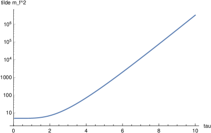
Figure 1: Plot versus $\tau$ of the mass parameter for axio-dilaton modes from 3-fluxes, $m_{f}^{2}(\tau),\ [\xi\simeq{5.25\ 10^{-2}/g_{s}}]$ in Eqs .(III.45) and (III.47) evaluated for $g_{s}=1.$

III.3 Predictions for warped modes masses and wave functions

The free parameters at our disposal consist of the string coupling constant and mass scale $g_{s}$ and $m_{s}$, the internal manifold warped volume $V_{W}=(2\pi L_{W})^{6}$, the 3-fluxes $M,\ K,\ [N=MK]$ and the warp factor for the mass hierarchy relative to the Planck mass scale, $w=m_{eff}/M_{\star}$. We choose $M_{\star}$ as the reference energy scale and express predictions in terms of the dimensionless geometric and flux parameters given by the ratio of bulk to throat radii $\eta=L_{W}/{\cal R}$ and Planck mass times and $AdS$ curvature, $z=M_{\star}{\cal R}=M_{\star}/k$. The string coupling constant is set at the value, $g_{s}=g_{D3}^{2}/(4\pi)\simeq 0.1$, appropriate to a $D3$-brane setup realizing a grand unified theory. The ratio parameters $\eta,\ z$ are naturally of $O(1)$, although we expect values well above unity upon matching predictions to data. For instance, the Chen-Tye study chen06 assigns values $\eta=10\ -\ 100$. The phenomenological analyses for the standard Randall-Sundrum models, using flat branes embedded in $AdS_{5}$ or $AdS_{5}\times S^{\delta}$ spacetimes, select values $z\in(10-\ 100)$ davoudheriz02 ; grzadgunion06 , with larger values $z=O(10^{4})$ required in the non-standard type gauge unification invoking the Weyl anomaly dienes99 . Large uncertainties also affect the Calabi-Yau volume parameter. For a fixed string compactification, it seems natural to identify the total warped volume $V_{W}$ (in Einstein frame) to the volume in the low energy effective action, setting ${\cal V}=V_{W}/\hat{l}_{s}^{6}=(L_{W}/l_{s})^{6}$. The analyses of $D3$-brane inflation kklmmt03 (after inserting the proper $(2\pi)$ factors) and those of electroweak supersymmetry breaking effects choi05 both favour the value $V_{W}^{1/6}/(2\pi l_{s})=L_{W}/l_{s}\simeq 5$. Larger values covering the wide range ${\cal V}\simeq(10^{5}-10^{30})$ are quoted in applications of the large volume scenario bala05 ; burgessSB06 ; spdealwis12 . The parameters satisfy the useful relations in Einstein frame,

$${w_{s}\over w}={M_{\star}\over m_{s}}={(L_{W}m_{s})^{3}\over\pi^{1/2}}=\sqrt{{\cal V}\over\pi}={(\eta z)^{3/4}\over\pi^{1/8}},\ \rho_{2}\equiv 2\bar{\rho}=e^{4u}={\cal V}^{2/3}=({V_{W}\over\hat{l}_{s}^{6}})^{2/3}=({L_{W}\over l_{s}})^{4}$$ (III.49)

$${\eta^{3}\over z}={\sqrt{\pi}\over\lambda_{N}^{4}g_{s}},\ \eta={m_{s}L_{W}\over\lambda_{N}g_{s}^{1/4}},\ z={M_{\star}\over m_{s}}\lambda_{N}g_{s}^{1/4}=m_{s}{\cal R}\sqrt{{\cal V}\over\pi},[{\cal R}=\lambda_{N}g_{s}^{1/4}l_{s},\ \lambda_{N}=({27\pi\over 4}N)^{1/4}].$$ (III.50)

The WKB approach that we use should hopefully be trustable in identifying the lightest charged Kaluza-Klein particles that sets the mass gap between Kaluza-Klein and moduli modes. The masses of radially excited modes (of fixed charges) grow linearly with the radial quantum number, $\hat{E}_{m_{n}}\sim n$, as is inferred from the limiting formula $n\simeq\int_{0}^{\tau_{0}}d\tau(-V_{eff})^{1/2}\sim E_{m}^{(n)}\int_{0}^{\infty}d\tau(I(\tau)/K^{2}(\tau))^{1/2}$, assuming that $\tau_{0}(\hat{E}_{m})$ recedes to infinity for large $\hat{E}_{m}$. The use of a truncated radial interval $0\leq\tau<\tau_{uv}$ with $\tau_{uv}\simeq 10$ has little effect on the accuracy of predictions since the region where the effective potential is sizeable does not extend far beyond the classical turning points, typically located at $\tau_{0}\leq 5-7$. Since the massive modes wave functions are concentrated near the throat apex, the estimates of masses and couplings are insensitive to the ultraviolet radial cutoff and justify using the throat domination case.

We evaluate the two unknowns $\hat{E}_{m}$ and $\tau_{0}$ by solving simultaneously the Bohr-Sommerfeld quantization condition, $\int_{0}^{\tau_{0}}d\tau(-V_{eff}(\tau))^{1/2}=(n-{1\over 4})\pi$, and the turning point equation, $V_{eff}(\hat{E}_{m}^{2},\tau_{0})=0$ in Eq. (III.27). In the presence of a repulsive wall producing an inner turning point $\tau^{\prime}_{0}>0$, one can extend the search procedure to the three unknowns $E_{m}^{2},\ \tau_{0},\ \tau^{\prime}_{0}$, by including the additional condition fixing the location of the inner turning point, $V_{eff}(\hat{E}_{m}^{2},\tau^{\prime}_{0})=0$, and matching the phase integral to $(n-{1/2})\pi$.

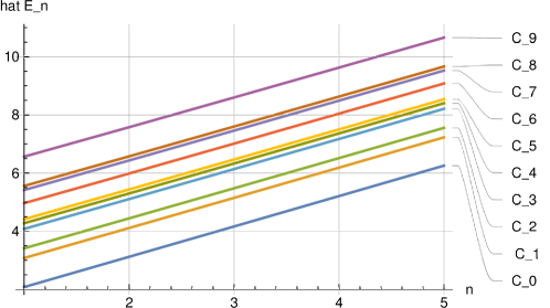
Figure 2: The reduced masses $\hat{E}_{m}$ of the ground and first four radial excitations of the 10 singlet and charged modes $C_{i}$ of the graviton field (Fig. 1) ordered according to increasing masses are plotted versus the radial excitation number $m+1=n=1,\cdots,4.$

The numerical applications were all performed with the help of ’Mathematica’ programming tools. For each of the graviton, 4-form scalar and axio-dilaton fields, we have selected 10 modes $C_{0},\cdots,\ C_{9}$ in low-lying representations of the isometry group. The mass spectra for the modes $C_{i}$, identified by their conserved charges $(j,\ l,\ r)$, are listed in Table 1 where we present results for the 4-d masses of ground states and first few radial excitations. The predicted masses are seen to increase with the angular momenta $j,\ l$, just like the 5-d masses $M_{5}^{2}$ but much less rapidly. The favoured candidate for the LCKP is the mode $S_{-}(jlr)=S_{-}(100)$ which saturates the unitary bound on $M_{5}^{2}$. The mass splittings are independent of the field types or the modes charges and grow linearly with the radial quantum number $\hat{E}_{m_{n}}\propto an$, as appears clearly on the plot of gravitons masses in Fig. 2 where $a\sim 1$. The scalar and axio-dilaton fields $S_{m},\ \tau_{m}$ feature a faster slope $a\simeq 1.5$.

It is useful to compare our predictions for gravitons to those using the full-fledged solutions in the deformed conifold throat pufu10 . Note that each $(j,l,r)$ mode in our case splits up into $2\tilde{j}+1$ sub-modes $(j,l)$ in the exact case labelled by $r\in(-\tilde{j},\cdots,\tilde{j}),\ [\tilde{j}=\min(j,l)]$. The comparison of our results for the sample of ground states masses, $\hat{E}_{m}\ [C_{0,1,2,3,4}]=[2.1,\ 3.1,\ 3.4,\ 5.0,\ 6.6]$ with the numerical results (averaged over $r$ values) from pufu10 , $(2(3/2)^{1/6}/(1.139)^{2})\times\hat{m}\ [C_{0,1,2,3,4}]\approx[1.7,\ 2.6,\ 3.0,\ 4.6,\ 5.9]$ show agreement to within $(20-10)\%$. To assess the impact of the deformed conifold geometry, we compare the reduced masses $\hat{x}_{m}$, defined by the formula $E_{m}=\hat{x}_{m}w/{\cal R}=\hat{x}_{m}M_{\star}w/z$, to the corresponding quantities $x_{m}$ in the undeformed conifold case, $E_{m}=x_{m}w/{\cal R}$ chemtob16 . Using Eq. (III.50), one finds the expression for the effective dimensionless masses,

$${\hat{x}_{m}}={2^{1/6}a_{0}^{1/4}z\hat{E}_{m}\over g_{s}^{1/4}(g_{s}M)^{1/2}{\cal V}^{1/6}}\sim({K\over g_{s}M})^{1/4}{\cal V}^{1/3}\hat{E}_{m}\sim|\ln w_{s}|^{1/4}{\cal V}^{1/3}\hat{E}_{m},$$ (III.51)

indicating an enhancement effect from stronger warping or larger compactification volume, relative to the (parameter independent) hard wall model $x_{m}$. We note for orientation that our prediction for the graviton ground state mass, $\hat{x}_{0}$, agrees with the value chemtob16 $x_{0}=3.83$ for ${\cal V}^{1/6}=5,\ g_{s}M=1$ and $z=O(10)$.

The effective potentials and wave functions for graviton modes are displayed in Fig.3 for illustrative cases. The attractive well regions in the potentials stem from the compensating contributions of the negative warping term $-\tilde{g}_{\tau\tau}h(\tau)E_{m}^{2}$ and the positive curvature term ${\cal G}_{1}(\tau)$, which dominate at small and large $\tau$, respectively. With increasing angular momentum, the turning points move to lower values $\tau_{0}\in(2-4)$. Although the calculations extend over the complete interval $\tau\in[0,\tau_{uv}],$ the masses and wave functions are chiefly sensitive to the inside well regions $0<\tau<\tau_{0}$. Deeper and narrower potential wells (with smaller turning points $\tau_{0}$) and more peaked wave functions occur for modes of larger masses $\hat{E}_{m}$. The flat potentials at $\tau>\tau_{0}$ causes the normalizable wave functions to decay exponentially at large distances. Note that the small discontinuities in the curves of wave functions is an artefact of our approximate matching prescription at turning points.

The comparison in Fig. 4 of the effective potentials in different modes reveals two novel features. Firstly, the inner well region for axio-dilaton modes is similar to that of graviton modes but the outer region receives additional contributions from 3-fluxes. The turning point location $\tau_{0}$ is significantly larger for lighter modes and it grows slowly with the radial excitation. For the $C_{1}$ graviton modes of radial charges $m=[0,1,2]$, $\tau_{0}=[3.13,4.59,5.57]$ and for the axio-dilaton modes $\tau_{0}=[2.62,3.42,3.84]$. Larger values occur for scalar modes. Secondly, the scalar modes $S_{-}$ feel a sloping potential near the origin stemming from the divergent term ${\cal G}_{1}\sim 1/\tau^{2}$. (This forces the choice $\delta_{W}=0$ in Eq. (III.27).) The repulsive wall overwhelms the attractive contribution from the warping term and the repulsive (or attractive) contributions from the 5-d mass term for $M_{5}^{2}>0$ (or $M_{5}^{2}<0$). The resulting inner turning point lies typically at $\tau^{\prime}_{0}\simeq(0.5\ -\ 1.)$ for $M_{5}^{2}>0$ and at $\tau^{\prime}_{0}\simeq(1.\ -\ 1.5)$ for $M_{5}^{2}<0$, while the outer turning point is pushed to larger values. The wide mass gap between the modes $S_{-}(C_{1})$ and $S_{-}(C_{4})$ is explained by the difference between 5-d masses ($M_{5}^{2}(C_{1})=-15/4,\ M_{5}^{2}(C_{4})=73/4$).

	GRAVITON $(h)$	SCALAR $(S_{-})$	DILATON $(\tau)$
Mode $(jlr)$	$\hat{E}_{n=0,1,2,3,4}$	$\hat{E}_{n=0,1,2}$	$\hat{E}_{n=0,1,2}$
$C_{0}(000)$	$2.08\ \ 3.11\ \ 4.16\ \ 5.20\ \ 6.25$	${1.90\ \ 3.06\ \ 4.17}$	${2.67\ \ 4.24\ \ 5.80}$
$C_{1}({1\over 2}{1\over 2}1)$	$3.07\ \ 4.10\ \ 5.14\ \ 6.18\ \ 7.22$	${0.66\ \ 1.56\ \ 3.04}$	${3.41\ \ 4.79\ \ 6.24}$
$C_{2}(100)$	$3.41\ \ 4.44\ \ 5.47\ \ 6.51\ \ 7.55$	${1.58\ \ 1.41\ \ 2.96}$	${3.69\ \ 5.02\ \ 6.43}$
$C_{3}(200)$	$4.96\ \ 5.98\ \ 7.01\ \ 8.04\ \ 9.07$	${2.20\ \ 3.34\ \ 4.44}$	${5.11\ \ 6.27\ \ 7.51}$
$C_{4}(300)$	${6.56\ \ 7.57\ \ 8.59\ \ 9.62\ \ 10.6}$	${4.17\ \ 5.22\ \ 6.26}$	${6.66\ \ 7.73\ \ 8.87}$
$C_{5}(212)$	${5.41\ \ 6.43\ \ 7.45\ \ 8.48\ \ 9.52}$	${2.79\ \ 3.89\ \ \ 4.96}$	${5.54\ \ 6.67\ \ 7.88}$
$C_{6}(112)$	${4.07\ \ 5.10\ \ 6.13\ \ 7.17\ \ 8.20}$	${0.79\ \ 2.06\ \ 3.35}$	${4.28\ \ 5.52\ \ 6.86}$
$C_{7}(110)$	${4.27\ \ 5.29\ \ 6.32\ \ 7.36\ \ 8.39}$	${1.00\ \ 2.35\ \ 3.55}$	${4.46\ \ 5.68\ \ 6.99}$
$C_{8}({3\over 2}{1\over 2}1)$	${4.41\ \ 5.43\ \ 6.46\ \ 7.49\ \ 8.53}$	${1.34\ \ 2.62\ \ 3.73}$	${4.59\ \ 5.80\ \ 7.09}$
$C_{9}(210)$	${5.55\ \ 6.57\ \ 7.59\ \ 8.62\ \ 9.66}$	${2.96\ \ 4.06\ \ \ 5.13}$	${5.68\ \ 6.80\ \ 8.00}$

Table 1: Reduced masses $\hat{E}_{n}$ for warped modes of the graviton $h$ real scalar $S_{-}$ and axio-dilaton $\tau$ fields  appearing in column entries, for a selection of ten singlet and charged states modes $C_{i},\ [i=0,\cdots,9]$ appearing in line entries. The sequences of masses for each mode refer to the ground state and first radial excitations labelled by $n$. The 5-d squared masses of the listed modes $C_{i}(jlr),\ [i=0,\cdots,9]$ are given for gravitons and axio-dilatons by $M_{5}^{2}(h,\tau)=H_{0}=(0,\ 8.25,\ 12,\ 36,\ 72,\ 45,\ 21,\ 24,\ 26.25,\ 48)$ and for $S_{-}$ eigenmodes by $M_{5}^{2}(S_{-})=H_{0}+16-8\sqrt{H_{0}+4}=(0,\ -3.75,\ -4,\ 1.40,\ 18.25,\ 5,\ -3,\ -2.33,\ -1.75,\ 6.31)$.

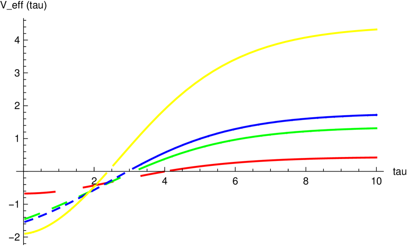
(a) Potential profiles $V_{eff}(\tau)$.

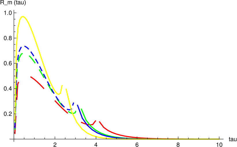
(b) Wave functions profiles $R_{m}(\tau)=B_{m}/\sqrt{G}$.

Figure 3: The radial effective potentials and (normalized) WKB wave functions for ground states of massive gravitons are plotted versus $\tau$. The red-green-blue-yellow coloured curves with dashes of decreasing sizes refer to the singlet and charged states $h(000),\ C_{1}({1\over 2}{1\over 2}1),\ C_{2}(100),\ C_{3}(200)$ of masses $\hat{E}_{m}=(2.07,\ 3.07,\ 3.41,\ 4.96)$.

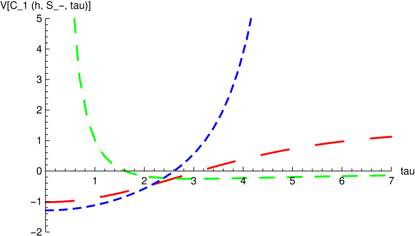
(a) $C_{1}({1\over 2}{1\over 2}1)$ mode.

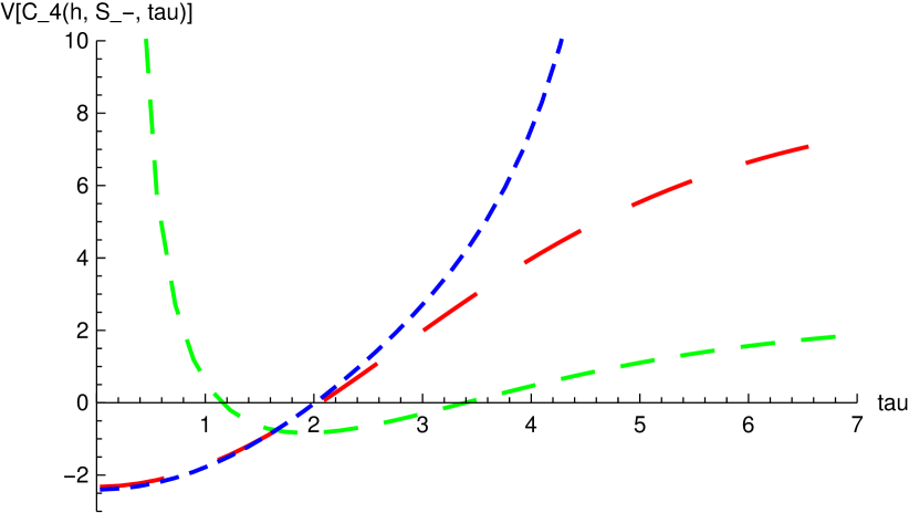
(b) $C_{4}(300)$ mode.

Figure 4: Plots versus $\tau$ of the effective potentials $V_{eff}(\tau)$ for charged modes of the graviton, scalar $S_{-}$ and axio-dilaton fields given by the red-green-blue coloured curves with dashes of decreasing sizes.

IV Interactions of warped modes

The information on warped modes interactions is nicely encoded within the supergravity action in Eq. (II.4). The coupling constants at tree level are given by the overlap integrals over ${\cal C}_{6}$ of wave functions products. We start the discussion with the cubic and higher order local couplings of graviton modes, discuss next how deformations of the classical warp profile $e^{-4A}$ caused by the conifold embedding in a compact manifold gandhi11 affect the cubic couplings and finally consider the graviton modes couplings to pairs of bulk 4-form scalar, axio-dilaton or geometric moduli modes and of $D3$-branes modes.

IV.1 Couplings of massive gravitons

The graviton modes couplings can be inferred from the perturbed 10-d curvature action,

$$S^{(2)}_{grav}={m_{D}^{8}\over 2}\int d^{4}x\sqrt{-(\tilde{g}_{4}+h)}\int d^{6}y\sqrt{\tilde{g}_{6}}e^{-4A(\tau)}\tilde{R}^{(4)}(\tilde{g}_{\mu\nu}+h_{\mu\nu}),$$ (IV.1)

by substituting the decomposition for the metric tensor fluctuations on the ground (real) and radially excited (complex) singlet and charged states of wave functions $\Psi_{m}(\tau,\Theta)$

$$h_{\mu\nu}(X)=\delta\tilde{g}_{\mu\nu}=\sum_{m}(h^{(m)}_{\mu\nu}(x)\Psi_{m}(\tau,\Theta)+\bar{h}^{(m)}_{\mu\nu}(x)\Psi^{\dagger}_{m}(\tau,\Theta)).$$ (IV.2)

The expansion in powers of the 4-d mode fields $h_{\mu\nu}^{(m)}(x)$ produces, in addition to the classical term $(M_{\star}^{2}/2)\int d^{4}x\sqrt{-\tilde{g}_{4}}\tilde{R}^{(4)}$ and the field equation term of linear order, the modes kinetic energy and mass terms along with their cubic and higher order mutual couplings which are expressed in the transverse-traceless gauge by the schematic formula, ignoring the spacetime structure of couplings,

$$\delta S_{grav}=\int d^{4}x\sqrt{-\tilde{g}_{4}}\int_{x}(\sum_{m}\lambda_{2}\bar{h}^{(m)\mu\nu}(\tilde{\nabla}_{4}^{2}-E_{m}^{2})h^{(m)}_{\mu\nu}+\sum_{(m_{i})}\lambda^{\prime}_{3}h^{(m_{1})}\partial h^{(m_{2})}\partial h^{(m_{3})}+\lambda^{\prime}_{4}h^{(m_{1})}h^{(m_{2})}\partial h^{(m_{3})}\partial h^{(m_{4})}+\cdots),$$ (IV.3)

$$[\lambda_{2}={1\over 4\kappa_{10}^{2}}={m_{D}^{8}\over 4}={M^{2}_{\star}\over 4V_{W}},\ \lambda^{\prime}_{n}={m_{D}^{8}{\cal R}^{3}J_{n}\over 8}={M^{2}_{\star}{\cal R}^{3}\over 8V_{W}}J_{n}={1\over 2}\lambda_{2}J_{n},\ J_{n}=\int d^{6}y\sqrt{\tilde{g}_{6}}e^{-4A(\tau)}\prod_{i=1}^{n}\Psi_{m_{i}}(\tau,\Theta)].$$ (IV.4)

The normalization condition in Eq. (III.23) sets the constant $\lambda_{2}$ and ensures that kinetic terms are diagonal while the numerical factor $1/2$ is due to the convention of summing over pairs of complex conjugate modes chemtob16 . The $n$-point coupling constants $\lambda^{\prime}_{n}$ are given by overlap integrals over the conifold volume of products of the participating modes wave functions. The transformation to canonically normalized fields, $h^{(m)}_{\mu\nu}\to h^{(m)}_{\mu\nu}/\sqrt{\lambda_{2}},$ replaces the $\lambda^{\prime}_{n}$ by the rescaled coupling constants,

$$\lambda_{n}=\lambda^{\prime}_{n}/\lambda_{2}^{n\over 2}={1\over 2}\lambda_{2}^{1-n/2}J_{n},\ [1/\sqrt{\lambda_{2}}=2\sqrt{V_{W}}/M_{\star}=2(2\pi)^{3}L_{W}^{3}/M_{\star}=2(2\pi)^{3}\eta^{3}{\cal R}^{3}/M_{\star}]$$ (IV.5)

which are assigned the energy dimensions $[\lambda_{n}]=E^{2-n}$. We consider the expression for the normalized modes wave functions, $\Psi_{m}={B_{m}(\tau)\Phi_{m}/(A\tilde{G}^{1/2}J)},\ [G(\tau)=\epsilon^{8/3}\ 2^{-4}\ \tilde{G}(\tau)]$ explicitly exhibiting the normalization integral $J$. It is then useful to factor out the dependence on parameters in the overlap integrals $J_{n}$ and $J$, hence expressing the coupling constants for canonically normalized fields in terms of new overlap integrals $\hat{J}_{n}$ and $J_{(m_{i})}$ as,

$$\lambda_{n}={1\over 2}\lambda_{2}^{1-n/2}J_{n}=(A^{2}\epsilon^{8/3}2^{-4})^{1-n/2}{\hat{J}_{n}\over\prod_{i=1}^{n}J_{(m_{i})}}=({2^{13/6}3^{1/2}\over\epsilon^{2/3}g_{s}M\alpha^{\prime}\sqrt{\lambda_{2}}})^{n-2}{\hat{J}_{n}\over 2\prod_{i=1}^{n}J_{(m_{i})}},$$ (IV.6)

$$[\hat{J}_{n}=\int d\tau d^{5}\Theta\sqrt{\tilde{\gamma}_{5}}{I(\tau)\tilde{G}(\tau)\over K^{2}(\tau)}\prod_{i=1}^{n}{B_{m_{i}}\Phi_{m_{i}}\over\sqrt{\tilde{G}(\tau)}},\ J_{(m)}=(\int d\tau{I(\tau)\over K^{2}(\tau)}|B_{m}|^{2}\int d^{5}\Theta\sqrt{\tilde{\gamma}_{5}}|\Phi_{m}|^{2})^{1/2}].$$ (IV.7)

We recall that the angular wave functions $\Phi_{m}$ are expressed in terms of trigonometric type polynomials related to Hypergeometric functions chemtob16 . Only the $\theta_{1},\ \theta_{2}$ polar angles integration are non-trivial, while those over azimuth angles $\phi_{1},\ \phi_{2},\ \psi$ implement the selection rules on magnetic quantum numbers imposed by the throat isometry, $\sum_{(i)}m_{j}^{(i)}=0,\ \sum_{(i)}m_{l}^{(i)}=0,\ \sum_{(i)}r^{(i)}=0$ modulo $Z$. This suggests factoring out the contribution from the three azimuth angles in $d^{5}\Theta$ and retaining only the angular integrals, $\int d^{5}\Theta\to\int_{0}^{\pi}d\theta_{1}\sin\theta_{1}\int_{0}^{\pi}d\theta_{2}\sin\theta_{2}$, in both the overlap and normalization integrals which are then denoted with primes, $\hat{J}_{n}^{\prime}$ and $J^{\prime}_{(m_{i})}$. The resulting formula for the $n$-point coupling constants reads

$$\lambda_{n}=({2^{13/6}3^{1/2}\over\epsilon^{2/3}g_{s}M\alpha^{\prime}\sqrt{\lambda_{2}}}\sqrt{4\over V_{X_{5}}})^{n-2}{\hat{J}^{\prime}_{n}\over 2\prod_{i}^{n}J^{\prime}_{(m_{i})}},\ [{\hat{J}_{n}\over\prod_{i}J_{(m_{i})}}=({V_{X_{5}}\over 4})^{1-n/2}{\hat{J}_{n}^{\prime}\over\prod_{i}J^{\prime}_{(m_{i})}},\ V_{X_{5}}={16\pi^{3}\over 27}].$$ (IV.8)

It is finally convenient to trade the $\lambda_{n}$ for reduced dimensionless coupling constants $\hat{\lambda}_{n}=O(1)$, extracting out the dependence on parameters by using the definition

$$\lambda_{n}=({\xi\eta^{3}\over M_{\star}w})^{n-2}\hat{\lambda}_{n},\ [\xi={2^{13/6}3^{1/2}\sqrt{4\over V_{X_{5}}}\over\epsilon^{2/3}g_{s}M\alpha^{\prime}\sqrt{\lambda_{2}}}{M_{\star}w\over\eta^{3}}={2^{19/6}3^{1/2}(2\pi)^{3}({{\cal R}\over\sqrt{\alpha^{\prime}}})^{3}\sqrt{4\over V_{X_{5}}}},\ \hat{\lambda}_{n}={w^{n-2}\hat{J}^{\prime}_{n}\over 2\prod_{i}^{n}J^{\prime}_{(m_{i})}}].$$ (IV.9)

The approximate relation for the ratio of 3-fluxes, $g_{s}M/K\simeq{2\pi\over 3}c_{2}=-2\pi/(3\ln(w_{s}\hat{\cal C}^{1/2}/{\cal V}^{1/6})),$ yields the useful formula for the auxiliary parameter $\xi$,

$$\xi=5.1\ 10^{3}\bar{\rho}^{1/4}({{\cal R}\over\sqrt{\alpha^{\prime}}})^{3}({K\over Mg_{s}})^{3/4}={5.1\ 10^{3}{\cal V}^{1/6}\over 2^{1/4}}(\lambda_{N}g_{s}^{1/4})^{3}(-{3\over 2\pi}\ln(w_{s}\hat{\cal C}^{1/2}/{\cal V}^{1/6}))^{3/4},\ [\hat{\cal C}=2^{1/3}a_{0}^{1/2}g_{s}M]$$ (IV.10)

which is seen to depend weakly on the flux and compactification volume parameters and to have a logarithmic dependence on the warp factor. For ${\cal V}^{1/6}=5,\ g_{s}M=1,\ w_{s}=10^{-4}$ and $\lambda_{N}g_{s}^{1/4}=1$, one finds the numerical value, $\xi\simeq 7.3\ 10^{4}$, which is significantly larger than the natural estimate $\xi=O(1)$ assigned in chen06 and lies well above the value $\xi=6\sqrt{12}\pi^{3/2}\simeq 1.15\ 10^{2}$ found in the undeformed conifold case chemtob16 . The resulting enhanced couplings for warped modes is a manifestation of the softer infrared geometry of the deformed conifold, as we discuss at the end of Subsection IV.4.

The couplings of massless and massive gravitons (denoted below by $g$ and $h$) differ significantly in size due to the orthogonality conditions on the wave functions and the fact that massless gravitons have constant wave functions. An examination of the overlap integrals shows that the massless gravitons couplings $g^{m-2}\partial g\partial g$ are independent of $w$, the massive and mixed massless-massive gravitons couplings behave as $h^{m-2}\partial h\partial h\sim 1/w^{m-2}$ and $h^{m-2}\partial g\partial g\sim 1/w^{m-4}$, while the single massive graviton couplings $hg^{m-3}\partial g\partial g$ vanish. We display in the table below order of magnitude (dimensional analysis) estimates for the amplitudes $\lambda_{M,N}$ and reaction cross sections $\sigma_{M,N}$ of the processes $g^{M},\ h^{N},\ h^{N}g^{M},\ [M,N\geq 2]$. In the pair annihilation cross sections, $\sigma(h^{2}\to h^{2})\sim({\xi/(M_{\star}w)})^{4}E_{h}^{2},\ \sigma(h^{2}\to hg)\sim({\xi/(M_{\star}w)})^{2}({E_{g}/M_{\star}})^{2}\hat{\lambda}_{3}^{2},$ the energy scale factors are set at the reaction energy $E_{h}^{2}\sim\max(E^{2},m_{K}^{2})$ for massive initial state modes and at $E_{h}^{2}\sim m_{K}^{2}$ for massless modes.

Configurations	$g^{M}$	$h^{N}$	$hg^{M}$	$h^{2}g$	$h^{3}g$	$h^{2}g^{2}$
Coupling Constant $\lambda_{M,N}$	${2^{M-3}\over M_{\star}^{M-2}}$	$({\xi\over M_{\star}w})^{N-2}$	$0$	${1\over M_{\star}}$	${\xi\over M^{2}_{\star}w}$	${2\over M^{2}_{\star}}$
Cross Section $\sigma_{M,N}$	${E_{g}^{2}\over M_{\star}^{2(M-2)}}$	$({\xi\hat{\lambda}\over M_{\star}w})^{2(N-2)}E_{h}^{2}$	$0$	${1\over M^{2}_{\star}}$	$({\xi\hat{\lambda}_{3}^{2}E_{g}\over M^{2}_{\star}w})^{2}$	${4E_{g}^{2}\over M_{\star}^{4}}$

The approximate matching of WKB wave functions at turning points confronts us with a technical difficulty in the numerical evaluation of overlap radial integrals $\hat{J}^{\prime}_{n}$. Since the turning points lie at mode dependent locations, a piece wise decomposition of the radial interval $\tau$ is required for modes of different masses. In practice, we limit the integration intervals for $J^{\prime}_{(m_{i})}$ to the inner region $\tau\leq\tau_{0}(E_{m_{i}})$ and account for the mode dependent locations of turning points in $\hat{J}^{\prime}_{n}$ by limiting the interval of integration to $\tau\in[0,\min(\tau_{0}(E_{m_{i}}))$. The reduced coupling constants for the 3- up to 6-point self interactions in allowed configurations $\hat{\lambda}_{3}(C_{0})^{q}C_{i}\bar{C}_{i},\ [C_{0}=h,\ i=1,\cdots,9,\ q=1,\cdots,4]$ are listed in Table 2. We see that predictions are not very sensitive to the participating modes charges and that the typical values for cubic couplings $\hat{\lambda}_{3}=O(10^{-1})$ decrease by a factor $2\ -\ 3$ at each unit incremental step in the number of coupled modes, $\delta q=1$.

Table 2: Reduced coupling constants $\hat{\lambda}_{2+q}$ for 3-, 4-, 5- and 6-order local couplings of massive gravitons in configurations $(h)^{q}C_{i}\bar{C}_{i},\ [i=1,\cdots,9]$ for $q=1,2,3,4$ singlet modes $h$ coupled to pairs of conjugate charged modes $[h=C_{0},C_{1},\cdots,C_{9}]$ listed in Fig. 1.

Couplings	$(h)^{q}hh$	$(h)^{q}C_{1}\bar{C}_{1}$	$(h)^{q}C_{2}\bar{C}_{2}$	$(h)^{q}C_{3}\bar{C}_{3}$	$(h)^{q}C_{4}\bar{C}_{4}$	$(h)^{q}C_{5}\bar{C}_{5}$	$(h)^{q}C_{6}\bar{C}_{6}$	$(h)^{q}C_{7}\bar{C}_{7}$	$(h)^{q}C_{8}\bar{C}_{8}$	$(h)^{q}C_{9}\bar{C}_{9}$
$q=1$	$0.128$	$0.158$	$0.165$	$0.191$	$0.209$	$0.197$	$0.17$	$0.182$	$0.184$	$0.198$
$q=2$	$0.0464$	$0.0717$	$0.0782$	$0.108$	$0.136$	$0.116$	$0.0917$	$0.0972$	$0.0988$	$0.118$
$q=3$	$0.00950$	$0.0150$	$0.0165$	$0.0236$	$0.0306$	$0.025$	$0.0197$	$0.0210$	$0.0214$	$0.0261$
$q=4$	$0.00405$	$0.00653$	$0.00723$	$0.0106$	$0.0140$	$0.0116$	$0.00871$	$0.00932$	$0.00951$	$0.0117$

IV.2 Throat deformation by compactification effects

The modification of the classical vacuum solution ($\Phi_{-}=0,\ G_{-}=0$) resulting from embedding the conifold in a compact Calabi-Yau manifold can affect the modes couplings. These effects are amenable to a perturbation theory description provided one restricts to radial distances in the throat region $0<\tau<\tau_{uv}$ intermediate between the horizon and boundary where deformations are small. Within the AdS/CFT duality approach of gandhi11 , the $x$-independent fluctuations of the various supergravity fields, $\varphi(y)=[\delta\Phi_{\pm}(y)=\delta(e^{4A}\pm\alpha(y)),\ \delta G_{\pm}(y),\delta g_{ab}(y),\ \delta\tau(y)]$, are split up into homogeneous and inhomogeneous parts. The homogeneous parts correspond to zero modes of the Laplace-Beltrami wave operators that one can then decompose on harmonic functions $Y^{\nu}(\Theta)$ of the conifold base $T^{1,1}$ times radial scaling functions $f_{\nu}(\tau)$ obeying same radial wave equations as the massless warped modes. Only the non-normalizable (NN) solutions for $f_{\nu}(\tau)$, which dominate in the ultraviolet, need be retained. The calculations in the large $\tau$ region, far from the conifold apex, can be conveniently carried out in terms of the conic radial variable, $r=3^{1/2}2^{-5/6}\epsilon^{2/3}e^{\tau/3}$. The decompositions of homogeneous parts on radial scaling functions,

$$\varphi(y)=\sum_{\nu}c^{NN}_{\nu}(\tau_{\star},\varphi)f_{\nu}(\tau,\varphi)Y^{\nu}(\Theta)\simeq\sum_{\nu}c^{NN}_{\nu}(r_{\star},\varphi)(r/r_{\star})^{\Delta_{\nu}(\varphi)-4}Y^{\nu}(\Theta),$$ (IV.11)

introduces the dimensions $\Delta_{\nu}(\varphi)$ for operators $O_{\nu}$ of the dual conformal gauge theory and the (floating) coefficients $c_{\nu}(r_{\star},\varphi)$, both depending on the field $\varphi$ type. The operators $O_{\nu}$ are selected among the class of (gauge invariant) composite operators of quantum number $\nu$ and the coefficients are expressed in terms of their unknown values at the ultraviolet scale $c_{\nu}(r_{uv},\varphi))$, using the radial scaling laws, $c_{\nu}(r_{\star},\varphi)/c_{\nu}(r_{uv},\varphi)=(r_{\star}/r_{uv})^{\Delta_{\nu}(\varphi)-4}$. The coupled field equations obeyed by the inhomogeneous source and mixing type fields fluctuations are solved iteratively by expanding the $\varphi(y)$ in powers of the small ratio $\tau_{\star}/\tau_{uv}$ (matching radius $\tau_{\star}$ over ultraviolet cutoff radius) and the warp factor $w$. Matching the solutions to small field deformations at the ultraviolet boundary $r_{uv}$ yields linear equations for the constant coefficients in these expansions that can be solved algebraically in terms of the $O(1)$ coefficients $c_{\nu}(r_{uv})$ describing the homogeneous parts. In practice, the coupled system of differential equations for inhomogeneous parts is of small dimensionality because the leading operators of lowest dimensions are few in numbers.

Since the coupling constants $\lambda_{n}$ of gravitons local interactions are evaluated from overlap integrals of the participating modes wave functions weighted by the warp profile, as in Eq. (IV.4), the leading corrections should arise from deformations of the warp profile, $\delta e^{-4A}=2\delta(\Phi_{-}+\Phi_{+})^{-1}$. Based on the available classification ceresole99 ; ceresoII99 of operators of the dual superconformal gauge theory in terms of the dimensions and supersymmetry character of deformations, the dominant contributions are those induced by fluctuations of the field $\delta\Phi_{-}$ which corresponds to the scalar modes $S_{-}$. The perturbed warp profile is then expressed at large radial distances by a sum over radial scaling terms,

$$\delta(e^{-4A(\tau,\Theta)})\simeq e^{-4A_{0}(\tau)}\sum_{\nu}c^{-}_{\nu}(r_{uv})w^{Q^{-}_{\nu}}({r\over{\cal R}})^{\Delta^{-}_{\nu}-4}Y^{\nu}(\Theta),\ [\Delta^{-}_{\nu}=-2+(4+H_{0}^{\nu})^{1/2}]$$ (IV.12)

where the ultraviolet coefficients $c^{-}_{\nu}(r_{uv})$ of $O(1)$ are corrected by warp factor powers $w^{Q^{-}_{\nu}}$ with index parameters $Q^{-}_{\nu}\geq 0$ set by the supersymmetry breaking character of the initial background produced by the gauge theory operators of dimensions $\Delta^{-}_{\nu}$. The $F$- or $D$-type operators in the highest superspace components ($\theta^{2},\ \theta^{2}\bar{\theta}^{2}$) of chiral or vector supermultiplets are unaffected ($Q^{-}_{\nu}=0$) while those in lower superspace components are assigned the power index $Q^{-}_{\nu}=2$ or 4. Details on the notations are provided in chemtob16 . The deformation effects on $e^{-4A(y)}$ can be taken into account by inserting inside the overlap integrals, denoted $J_{n}$ in Eq. (IV.4), the spurion modes wave functions $f_{\nu}(\tau)Y^{\nu}(\Theta),\ [f_{\nu}(\tau)\simeq r^{\Delta_{\nu}^{-}-4}]$. These effects modify the selection rules imposed by the throat isometry in an easily identified way by allowing otherwise forbidden couplings. The reduced dimensionless coupling constants for the deformed couplings $\hat{\lambda}_{n}$ can be defined in a similar fashion as Eq. (IV.8),

$$\lambda_{n}=c_{\nu}w^{-4+\Delta^{-}_{\nu}+Q^{-}_{\nu}}\lambda^{\prime}_{n},\ \ \lambda^{\prime}_{n}\simeq(5.1\ 10^{3}{\eta^{3}(N/M^{2})^{3/4}\bar{\rho}^{1/4}\over wM_{\star}g_{s}^{3/4}})^{n-2}\hat{\lambda}_{n}.$$ (IV.13)

The leading contributions to $\delta\Phi_{-}$ arise from supersymmetry breaking operators in lowest components of vector supermultiplets, $Q^{-}_{\nu}=4$, whose dimensions $\Delta^{-}_{\nu}$ increase with the modes charges. The coupling constants of the cubic interactions $(hhC_{i}),\ [i=1,\cdots,9]$ which vanish in the undeformed background case, take the finite values displayed in Table 3.

Table 3: Coupling constants of the cubic local couplings $hhC_{i},\ [i=0,1,\cdots,9]$ induced through the warp profile perturbation $\delta(e^{-4A(r,\Theta)})$ due to compactification effects. The deformed coupling constants $\hat{\lambda}_{3}$ are given by overlap integrals involving products of wave functions for the participating modes and for the spurion harmonic modes $\delta\Phi_{-}^{\nu_{i}}(\bar{C}_{i})$ needed to neutralize the total charge. The warp factor dependent factors $w^{-4+\Delta^{-}_{\nu}+Q^{-}_{\nu}}$ are determined by the supersymmetry breaking parameter, which is set at $Q^{-}_{\nu_{i}}=4$ in all cases, and the dual gauge theory operator dimension $\Delta^{-}_{\nu_{i}}(S_{-})$ which is mode dependent. The unknown constant coefficients ${1\over 2}\hat{c}^{-}_{\nu}=O(1)$ were factored out. The power index of $w$ is determined by the dimensions, by $\Delta^{-}_{\nu_{i}}(S_{-})=-2+(H_{0}+4)^{1/2}=(0,\ 1.5,\ 2,\ 4.32,\ 6.71,\ 5,\ 3,\ 3.29,\ 3.5,\ 5.21)$.

Couplings	$C_{0}C_{0}C_{0}$	$C_{0}C_{0}C_{1}$	$C_{0}C_{0}C_{2}$	$C_{0}C_{0}C_{3}$	$C_{0}C_{0}C_{4}$	$C_{0}C_{0}C_{5}$	$C_{0}C_{0}C_{6}$	$C_{0}C_{0}C_{7}$	$C_{0}C_{0}C_{8}$	$C_{0}C_{0}C_{9}$
$\hat{\lambda}_{3}/(-{1\over 2}\hat{c}^{-}_{\nu})$	$0.00761$	$0.0180w^{3/2}$	$0.0235w^{2}$	$0.0747w^{4.3}$	$0.208w^{6.71}$	$0.101w^{5}$	$0.0394w^{3}$	$0.0458w^{3.29}$	$0.0505w^{3.5}$	$0.111w^{5.21}$

IV.3 Gravitons couplings to bulk scalar modes

The interactions between different types of warped modes can be computed at tree level by applying the familiar perturbation theory rules to the action in Eq. (II.4). The metric tensor field couplings are encoded within the universal type operator, $h^{(m)\mu\nu}T_{\mu\nu}$, proportional to the energy-momentum stress tensor. For a single graviton mode $h^{(m)}_{\mu\nu}$ coupled to pairs of scalar modes $b^{(m)}(x)$ from the 4-form field in Eqs. (III.29) and (III.38), the effective Lagrangian for canonically normalized fields is given by,

$$L_{EFF}=\lambda_{m_{1}m_{2}n}^{b}h^{(n)\mu\nu}\partial_{\mu}b^{(m_{1})\dagger}\partial_{\nu}b^{(m_{2})},$$ (IV.14)

$$[\lambda_{m_{1}m_{2}n}^{b}={1\over 2\sqrt{\lambda_{2}}}{\int d\tau d^{5}\Theta{\sqrt{\tilde{g}_{6}}e^{4A}Q(\tau)\over{\cal G}(\tau)G^{1/2}(\tau)}\tilde{b}_{m_{1}}\tilde{b}_{m_{2}}B_{n}(\tau)\ \Phi_{m_{1}}^{\dagger}\Phi_{m_{2}}\Phi_{n}\over(\prod_{i=1,2}\int d\tau\int d^{5}\Theta{\sqrt{\tilde{g}_{6}}e^{4A}Q(\tau)\over{\cal G}(\tau)}|\tilde{b}_{m_{i}}\Phi_{m_{i}}|^{2})^{1/2}(\int d\tau d^{5}\Theta{\sqrt{\tilde{g}_{6}}e^{-4A}\over G(\tau)}|B_{n}\Phi_{n}|^{2})^{1/2}}].$$ (IV.15)

Although the wave functions of scalar modes $S^{-}_{m}$ differ widely from those of gravitons, we anticipate that this is compensated by the different measure factor in overlap integrals. The expectation that the strengths are comparable to those of gravitons self couplings, $\lambda_{3}^{b,t}\simeq\lambda_{3}$, can be verified by analyzing the overlap integrals at small $\tau$ and is also borne out from the hard wall model case chemtob16 .

The couplings of graviton modes to pairs of axio-dilaton mode fields $t^{(m)}(x)$, of wave equations given by Eq. (III.44), have same overlap integrals as those for the graviton modes self couplings in Eq. (IV.7). The effective Lagrangian for trilinear couplings of canonically normalized modes is given by

$$L_{EFF}=\lambda_{m_{1}m_{2}n}^{t}h^{(n)\mu\nu}\partial_{\mu}t^{(m_{1})\dagger}\partial_{\nu}t^{(m_{2})},$$ (IV.16)

$$[\lambda_{m_{1}m_{2}n}^{t}={1\over 2\sqrt{\lambda}_{2}}{\int d\tau{I(\tau)\over K^{2}(\tau)}\tilde{t}_{m_{1}}\tilde{t}_{m_{2}}B_{n}(\tau)\int d^{5}\Theta\sqrt{\tilde{\gamma}_{5}}\Phi_{m_{1}}^{\dagger}\Phi_{m_{2}}\Phi_{n}\over\prod_{i=1,2}(\int d\tau d^{5}\Theta{\sqrt{\tilde{g}_{6}}e^{-4A}\over G(\tau)}|\tilde{t}_{m_{i}}\Phi_{m_{i}}|^{2})^{1/2}(\int d\tau d^{5}\Theta{\sqrt{\tilde{g}_{6}}e^{-4A}\over G(\tau)}|B_{n}\Phi_{n}|^{2})^{1/2}}]$$ (IV.17)

where $\lambda^{t}$ are expected to be comparable to those of graviton modes self couplings. The interactions of the geometric (complex structure and Kähler) moduli can be inferred in a similar way starting from the reduced kinetic action, as discussed in chemtob16 . Nevertheless, the information on the moduli wave functions is still uncertain in spite of the insights provided in the initial studies dougba07 ; dougtorr08 ; freyroberts13 . For instance, the Kähler metric for the complex structure modulus $S$ is found to acquire a divergent contribution $G_{S\bar{S}}\sim 1/S$ near the point $S=0$ of the moduli space where the deformed conifold 3-cycle collapses dougba07 ; dougtorr08 . The predictions for radial profiles of the universal volume modulus mixing with the metric tensor, $c(x)-g_{MN}(x)$, derived in the deformed conifold within the gauge compensator approach frey08 , $\delta_{c}g_{\mu\nu}\sim r^{2}/N^{1/2},\ \delta_{c}g_{rr}\sim N^{1/2}/r^{2}$, differ from the naive classical estimates inferred from expanding the warp profile ansatz at large radial distances, $\delta_{c}g^{(0)}_{\mu\nu}\sim r^{6}/N^{3/2},\ \delta_{c}g^{(0)}_{rr}\sim r^{2}/N^{1/2}$.

IV.4 Couplings of gravitons to $D3$-branes

We consider next the interactions between bulk and brane fields mirrors the string theory couplings between closed and open strings. The scalar and Majorana-Weyl spinor massless fields, $X^{M}(\xi)$ and $\Theta(\xi)$, describing the $Dp$-brane world volume embedding in super-spacetime $M_{10}$, couple to the pull-back transforms of the bulk supergravity multiplet fields. The action principle for superbranes is formulated using the invariance under diffeomorphisms of the world volume $M_{p+1}$ intrinsic coordinates $\xi^{\alpha},\ [0,1,\cdots,p]$ and local Lorentz-Poincaré, supersymmetry and fermionic $\kappa$-symmetry groups. We shall consider $D3$-branes located at points of $X_{6}$ using the general formalism developed in marino99 ; gauntlett03 ; martucci05 ; lustmartsim08 and applied in marche08 ; marche10 ; chemtob16 . The couplings of massive graviton field modes $h^{(m)}_{\mu\nu}(x)$ to bosonic and fermionic massless field modes $\varphi^{m}=X^{m}/(2\pi\alpha^{\prime}),\ \psi^{m}$ of $D3$-branes are set by the graviton wave function value at the brane location, $y=y_{\star}=(r_{\star},\ \Theta_{\star})$. The dimension $5$ effective Lagrangian contributed by the Born-Infeld action chemtob16 for fields of canonical kinetic energy is given by

$$\delta S(D3)=-{\lambda_{3}^{B}\over\sqrt{2}}\int d^{4}x\sqrt{|\tilde{g}_{4}|}\ h_{\mu\nu}^{(m)}(x)\tilde{g}_{np}(\partial^{\mu}\varphi^{n}\partial^{\nu}\varphi^{p}+i\bar{\psi}^{n}\partial_{\mu}\gamma_{\nu}\psi^{p}),\ \lambda_{3}^{B}=\sqrt{2}{2^{13/6}3^{1/2}\over g_{s}M\alpha^{\prime}\epsilon^{2/3}\sqrt{\lambda_{2}}}\Psi_{m}(y_{\star}),$$ (IV.18)

$$[{1\over\sqrt{\lambda_{2}}}={2\sqrt{V_{W}}\over M_{\star}}={2(2\pi L_{W})^{3}\over M_{\star}},\ \Psi_{m}(y_{\star})={B_{m}(\tau_{\star})\Phi_{m}(\Theta_{\star})\over\tilde{G}^{1/2}J_{(m)}}].$$ (IV.19)

One can use the familiar definition of the effective action for a graviton field $h_{\mu\nu}$ coupled to a scalar matter field $\phi$ to evaluate the two-body decay rates of gravitons, using the identification, $1/M_{\star}\to\lambda_{3}^{B}$,

$$\delta S(D3)={1\over M_{\star}\sqrt{2}}\int d^{4}xh^{\mu\nu}T_{\mu\nu}(\phi)\ \Longrightarrow\ \Delta\Gamma(h\to\phi+\phi)\simeq{m_{h}^{3}\over 960\pi M_{\star}^{2}}(1-{4m_{\phi}^{2}\over m_{h}^{2}})^{1/2}.$$ (IV.20)

It is convenient to define a reduced dimensionless coupling constant $\hat{\lambda}_{3}^{B}=O(1)$, similar to the prescription used previously for bulk modes in Eq. (IV.9),

$$\lambda_{3}^{B}={\xi^{B}\eta^{3}\over M_{\star}w}\hat{\lambda}_{3}^{B},\ \ [\hat{\lambda}_{3}^{B}={wB_{m}(\tau_{\star})\Phi_{m}(\Theta_{\star})\over\tilde{G}^{1/2}(\tau_{\star})J^{\prime}_{(m)}},\ \xi^{B}=\sqrt{2}{2^{13/6}3^{1/2}2(2\pi)^{3}{\cal R}^{3}\over\epsilon^{2/3}g_{s}M\alpha^{\prime}}\sqrt{4\over V_{X_{5}}}=\sqrt{2}\xi]$$ (IV.21)

with $\xi^{B}=\sqrt{2}\xi\approx 10^{5}.$ For $D3$-branes near the conifold apex $\tau_{\star}=0$, the numerical values for $\hat{\lambda}^{B}_{3}$ are listed in Table 4 for four cases associated to different locations in the base manifold. The variations between Cases $I,II,III$ reflect on the dependence of charged graviton wave functions $C_{i}$ on the base manifold angles. Note that the harmonic wave functions for modes $C_{1,5,6,8}$ of charge $r_{i}\neq 0$ vanish at the pôles $\theta_{1,2}=0$ and those of singlet modes are angle independent. In the smeared distribution Case $IV$, the couplings have the anticipated smooth dependence on modes charges.

The effective 4-d gravitational mass scale for $D3$-branes localized at $\tau_{\star}$, usually defined by the ratio $\Lambda_{KK}=M_{\star}/\Phi_{m}(\tau_{\star})$, can also be evaluated from the formula, $\Lambda_{KK}\simeq 1/\lambda_{3}^{B}=M_{\star}w/(\xi^{B}\hat{\lambda}_{3}^{B}\eta^{3})$. For $\xi^{B}=10^{5},\ \hat{\lambda}_{3}^{B}=10^{-2},\ w=10^{-14},$ one finds the rather small value $\Lambda_{KK}\sim 10^{-2}/\eta^{3}$ TeV. The further strong suppression from $\eta>>1$ might be compensated if the brane were located at a finite distance from the tip. The predicted mass scale lies well below that found in studies using Randall-Sundrum model, $\Lambda_{KK}\approx 51$ TeV, the undeformed conifold background chemtob16 , $\Lambda_{KK}\approx 19$ TeV, and the softened warp profile model shiuetal07 ; guirkshiuzur07 , $\Lambda_{KK}\approx 2$ TeV, for the same value of $w$.

Table 4: Reduced coupling constants for bulk graviton modes $h,\ C_{i},\ [i=1,\cdots,9]$ coupled to pairs of $D3$-brane modes in four distinct choices for the brane location in the base manifold, all using vanishing azimuthal angles $\phi_{1}=\phi_{2}=\psi=0$. Case $I$ refers to polar angles $\theta_{1}=0,\ \theta_{2}=0$, Case $II$ to $\theta_{1}=2\pi/5,\ \theta_{2}=0,$ Case $III$ to $\theta_{1}=\theta_{2}=\pi/5,$ and Case $IV$ to smeared distributions averaged over $\theta_{1}$ and $\theta_{2}$.

	$h$	$C_{1}$	$C_{2}$	$C_{3}$	$C_{4}$	$C_{5}$	$C_{6}$	$C_{7}$	$C_{8}$	$C_{9}$
$\hat{\lambda}_{3}^{B}(I)$	0.022	$0.39\ 10^{-4}$	0.077	$0.15$	$0.25$	0.	$0.$	$0.18$	$8.\ 10^{-4}$	0.30
$\hat{\lambda}_{3}^{B}(II)$	0.022	$0.32\ 10^{-4}$	0.023	0.056	0.10	0.	$0.$	$0.055$	$0.$	0.11
$\hat{\lambda}_{3}^{B}(III)$	0.022	0.053	0.062	0.075	0.027	0.08	0.075	0.	0.083	0.
$\hat{\lambda}_{3}^{B}(IV)$	0.022	0.035	0.038	0.060	0.084	0.059	0.041	0.044	0.052	0.060

V Rôle of warped modes in early universe cosmology

The discussion of $D3$-branes moving in Klebanov-Strassler type background deformed by the presence of $\bar{D}3$-branes near the deformed conifold apex has provided useful insights on the slow roll inflation scenario kklt03 ; baumann06 ; baumann08 . The energy released through $D3-\bar{D}3$-branes annihilation is assumed to produce at inflation exit massive closed strings fastly decaying to massless closed strings lambert03 that produce massless particles and massive Kaluza-Klein modes kofman05 ; chialva05 ; chen06 ; kofman08 . Based on the information collected so far, we wish to examine whether the gas of warped modes present in the throat could provide an attractive mechanism for the post-inflation universe reheating in this context. The resulting system of multiple species of metastable particle coupled by gravitational interactions at effective scales lying well below the Planck mass scale should hopefully have a predictable thermal evolution.

V.1 Preliminary considerations

We assume that the exit from inflation leads to a Friedman-Robertson-Walker (FRW) universe filled by a gas of relativistic Kaluza-Klein warped modes localized in the inflationary throat, called hereafter $A$-throat. The radiation dominated regime is characterized by the scaling laws for the temperature, Hubble rate and energy density as a function of cosmic time, $T\propto a^{-1}\propto t^{-2},\ H\equiv\dot{a}(t)/a=1/(2t),\ \rho=3M_{\star}^{2}/(4t^{2})$. We shall use the simplified formulas for the particles masses $m_{K}=x_{m}w/{\cal R}$ and couplings $\lambda_{n}h^{n-2}\partial h\partial h,\ [\lambda_{n}\propto 1/(M_{\star}w)^{n-2}]$ depending on the $A$-throat warp factor and curvature radius parameters, $w$ and ${\cal R}$. The statistical number of degrees of freedom, counting the number of degenerate harmonic modes in $T^{1,1}$, is described by the temperature dependent Chen-Tye ansatz chen06 , $g^{b}_{\star}(T)=\theta(T-m_{K})(T/(w/{\cal R}))^{\gamma},\ [\gamma=5]$. In case the $A$-throat also hosts Standard Model $D3$-branes, this is combined with (or replaced by) the (constant) number of massless brane modes, $g^{SM}_{\star}(T)\sim O(100)$.

The initial temperature and cosmic time $T_{I},\ t_{I}$ can be determined by matching the energy density $\rho_{K}(t)=(\pi^{2}g_{\star}/30)T^{4}(t)$ of the relativistic gas to that deduced from the Hubble expansion rate at inflation exit, $\rho_{I}(t)=3M_{\star}^{2}H^{2}(t),\ [H(t)=1/(2t)]$. Assuming that the energy released through either $D\bar{D}$-brane annihilation at time $t_{I}$, or massive closed strings decays at time $t_{I}+\Delta t_{S}$, is efficiently transferred to warped modes, one obtains the balance equation,

$$\rho_{I}(t)\equiv{3M_{\star}^{2}\over 4t^{2}}=\rho_{K}(t)\equiv{\pi^{2}g_{\star}\over 30}T^{4}(t),\ [t=t_{I}+\Delta t_{S}].$$ (V.1)

The temperature at time $t_{I}$ can be explicitly determined in two limits which we examine in turn for a constant $g_{\star}(T)$. If the energy from by $D3-\bar{D}3$ annihilation is transferred instantaneously, $\Delta t_{S}=1/\Delta\Gamma_{S}<<t_{I}$, then equating $\rho_{K}(t_{I})$ to $\rho_{I}(t_{I})\simeq 2N_{A}\tau_{3}w^{4}={4\pi N_{A}w^{4}/\hat{l}_{s}^{4}}$, where $N_{A}$ is the 5-form flux supported by the $A$-throat, can be used to determine the initial temperature and time,

$$T_{I}=({90\over 4\pi^{2}g_{\star}})^{1/4}\sqrt{M_{\star}\over t_{I}}\simeq({2N_{A}\tau_{3}w^{4}\over 3M_{\star}^{2}})^{1/4}\ \Longrightarrow\ {T_{I}\over M_{\star}}\simeq 0.51\ w({N_{A}\over g_{\star}(\eta z)^{3}})^{1/4}\simeq 1.57\ 10^{-7}N_{A}^{1/4}{w\over 10^{-4}}({10^{4}\over\eta z})^{3/4}.$$ (V.2)

If the decay lifetime is larger that the Hubble time, $t_{I}<<\Delta t_{S}$, then using the estimate for the total decay rate of massive closed strings chialva05 , $\Delta\Gamma_{s}(S\to K+K)=c^{\prime}_{KK}g_{s}wm_{s},$ one can evaluate the reheat temperature,

$$T_{RH}\simeq({90\over 4\pi^{2}g_{\star}})^{1/4}\sqrt{M_{\star}\Delta\Gamma_{S}}\ \Longrightarrow\ {T_{RH}\over M_{\star}}=({90\pi^{1/4}\over 4\pi^{2}})^{1/4}{(c^{\prime}_{KK}g_{s}w^{1/2}\over g_{\star}^{1/4}(\eta z)^{3/8}}\simeq 0.31\ 10^{-6}({w\over 10^{-4}}{c^{\prime}_{KK}\over 10^{-4}})^{1/2}({10^{4}\over\eta z})^{3/8}.$$ (V.3)

The numerical results in Eqs. (V.2) and (V.3) were obtained for $g_{s}=0.1,\ g_{\star}=100$ setting $c^{\prime}_{KK}=10^{-4}$ chialva05 which is numerically close to the estimate $c^{\prime}_{KK}\simeq g^{3}_{s}$ kofman05 . The two predictions for the initial temperature are sensitive to the warp factor, have acceptable magnitudes and satisfy the relationship, $\sqrt{T_{I}}/T_{RH}\approx 1.3\ 10^{3}N_{A}^{1/8}$. Had one used instead the statistical factor ansatz, $g_{\star}(T)=(T/\alpha)^{\gamma},\ [\alpha=w/{\cal R}]$, the resulting reheat temperature, expressed in terms of that for $g_{\star}=100$ as, $({T_{RH}\over M_{\star}})\simeq(\sqrt{10}({w\over z})^{\gamma\over 4(\gamma+4)})({T_{RH}\over M_{\star}})^{1\over\gamma+4}$, reaches the excessively large value, $({T_{RH}\over M_{\star}})\approx 10^{-5/2}$ for $z=10^{3},\ \gamma=5$.

We wish to study in this Section the thermal evolution of warped modes in the twofold goal of determining their ability to thermalize and leave a cold thermal relic component. The answer clearly depends on whether the Standard Model branes setup is located in the $A$-throat or, if a fraction of modes can stream out of the $A$-throat, in the Calabi-Yau bulk or in another distant throat. We consider two main cases along same lines as chen06 . The single throat case in Subsection V.2 deals with an $A$-throat accommodating both inflation and the Standard Model and the double throat case in Subsection V.3 assumes the existence of an additional $S$-throat hosting the Standard Model branes near its apex.

A few preliminary remarks are in order before moving on to the main discussion. In the context of 10-d supergravity, the cosmic bath consists of infinite towers of massive particle species differing by the spin $\leq 2$, the charge under the throat isometry group and the radial excitation. The tree level action includes cubic and higher order couplings that can induce decay channels for most modes. The fate of massive modes depends on how their decay rates $\Gamma_{1\to 2}$ compare to the Hubble expansion rate $H(t)$. For instance, the decay rates for massive gravitons with ${\cal F}$ open channels of conjugate pairs of modes $\phi$, inferred from Eq. (IV.20),

$${\Delta\Gamma(h\to\phi+\bar{\phi})\over(1-4m_{\phi}^{2}/m_{h}^{2})^{1/2}}\approx{\lambda_{3}^{2}m_{h}^{3}{\cal F}\over 960\pi}\simeq{x_{m}^{3}\xi^{2}M_{\star}\over 960\pi}{\hat{\lambda}_{3}^{2}\eta^{6}w{\cal F}\over z^{3}},$$ (V.4)

yield the estimates $\Delta\Gamma\sim O(10^{27})\ GeV$, for $x_{m}=3.83,\ \eta=100,\ z=10,\ {\cal F}=100,\ w=w_{A}=10^{-4}$. The resulting lifetime $\Delta t_{1\to 2}=O(10^{-52})\ s$ is comparable to the estimate $O(10^{-49})\ s$ of kofman05 but considerably shorter than the lifetime of massive closed strings $O(10^{-33})\ s$ or the inflation exit time, $t_{I}=\sqrt{3}\pi^{5/4}(\eta z)^{3/2}/(w^{2}M_{\star}^{-1})\simeq O(10^{-30})\ s$. The gravitons decays to pairs of brane modes are of same size up to large uncertainties due to the dependence on the brane location.

Similar conclusions hold for 2-body decays between neighbour radially excited graviton modes, $\Gamma_{1\to 2}(h_{m_{n}}\to h_{m_{n-1}}+\bar{h}_{m_{n-1}})$, given the comparable ratios of coupling constants chemtob16 , $\lambda_{3}(h_{1}hh)/\lambda_{3}(hhh)\simeq 0.2/0.5$ and the smaller ratios $\lambda_{3}(h_{2}hh)/\lambda_{3}(hhh)\simeq 0.04/0.5$ for non-sequential decays. We also note that the axio-dilatons have similar couplings as gravitons while the scalars $S^{-}$ have suppressed couplings. The contributions from deformation effects to disallowed couplings are suppressed by powers of the warp factor. If massless modes were present in the mass spectrum in addition to the graviton, one expects their couplings to be $O(1/M_{\star})$ suppressed, hence causing an early decoupling from the thermal bath with a tiny primordial abundance. Their delayed production through pair annihilations of massive gravitons, $h+h\to g+g,\ h+g\to g+g,$ is expected chen06 to contribute a small radiation component today of order $(g_{\star}/g_{s})^{1/4}(m_{s}w/M_{\star})$. We conclude from the above discussion that the excited warped modes should fastly decay to a population of weakly interacting ground state modes formed mostly from graviton and scalar singlet modes. This should justify focusing on a simplified treatment of the thermal evolution restricted to a single species of graviton modes.

V.2 Single throat case

We begin with the case of a single deformed conifold throat hosting both $D3-\bar{D}3$-brane inflation kklmmt03 and the Standard Model, using the warp factor value $w=w_{A}=10^{-4}$ that reproduces the expected value of the Hubble rate at inflation exit, $H_{I}\sim 10^{-4}M_{\star}$. For Standard Model $D3$-branes located near the conifold apex, the ultraviolet cutoff mass scale lies near the grand unified theory (GUT) value, $M_{GUT}\simeq wM_{\star}$. Recall that the throat thermalization is realized as long as the elastic and inelastic scattering rates exceed the Hubble expansion rate $H(T)$. We examine this possibility by considering pair annihilation among bulk modes and decay of bulk modes to pairs of brane modes controlled by $2\to 2$ and $1\to 2$ processes, respectively, described by the dimensional analysis estimates of the rates,

$$\Delta\Gamma_{2\to 2}={g_{K}{\cal F}\zeta(3)\over\pi^{2}}\lambda_{3}^{4}T^{5}=1.73\ 10^{20}\hat{\lambda}_{3}^{4}{T^{5}\eta^{12}\over M_{\star}^{4}w^{4}},\ \Delta\Gamma^{B}_{1\to 2}={{\cal F}^{\prime}\lambda_{3}^{2}m_{K}^{3}\over 960\pi}=1.19\ 10^{9}\hat{\lambda}_{3}^{2}{M_{\star}w\eta^{6}\over z^{3}},$$ (V.5)

where ${\cal F},\ {\cal F}^{\prime}$ count the numbers of open channels and the numerical values were obtained from the input data, $x_{m}=3.83,\ {\cal F}=10,\ {\cal F}^{\prime}=10,\ \zeta(3)=1.202,\ \xi=7.3\ 10^{4},\ \xi^{B}=\sqrt{2}\xi\approx 10^{5}$. The Hubble rate $H(T)=(\rho(T)/(3M_{\star}^{2}))^{1/2}=(\pi^{2}g_{\star}/90)^{1/2}T^{2}/M_{\star}\simeq 0.33g_{\star}^{1/2}T^{2}/M_{\star}$ is evaluated with $g_{\star}(T)\simeq 100$. The resulting conditions for bulk or brane thermalization as a function of the temperature scaled by the modes mass $T_{K}=T/m_{K}$ are then given by

$$1<R(T)={\Delta\Gamma_{2\to 2}\over H(T)}=C_{R}{\eta^{12}T_{K}^{3}\over wz^{3}},\ [C_{R}={(\xi\hat{\lambda}_{3})^{4}x_{m}^{3}g_{K}\zeta(3){\cal F}\over\pi^{2}(0.33g_{\star}^{1/2})}\simeq 2.91\ 10^{21}\hat{\lambda}_{3}^{4}]$$ (V.6)

$$1<\Delta^{B}(T)={\Delta\Gamma^{B}_{1\to 2}\over H(T)}=C_{B}{\eta^{6}\over wzT_{K}^{2}},\ [C_{B}={(\xi_{B}\hat{\lambda}_{3}^{B})^{2}x_{m}{\cal F}^{\prime}\over 960\pi(0.33g_{\star}^{1/2})}\simeq 3.8\ 10^{7}\hat{\lambda}_{3}^{B2}].$$ (V.7)

It makes sense to examine the variations of these ratios in the interval $T_{K}\in[0.1,\ 10]$. Writing the parameter dependence as, $R(T)\propto(\eta^{3}/z)^{3}\eta^{3},\ \ \Delta^{B}(T)\propto(\eta^{3}/z)\eta^{3},$ we realize that both ratios are proportional to powers of the parametrically small ratio, $\eta^{3}/z=\sqrt{\pi}/(\lambda_{N}^{4}g_{s})\sim 1/(g_{s}N)$, times the same factor $\eta^{3}$. The plots of $R(T),\ \Delta^{B}(T)$ in Fig. 5 at a discrete set of values of $\eta^{3}/z$ with $\eta=1$ should give lower bounds for these quantities. We see that both ratios lie comfortably above unity, with the ratio $R(T)/\Delta^{B}(T)>>1$ meaning that the throat thermalization well precedes brane thermalization.

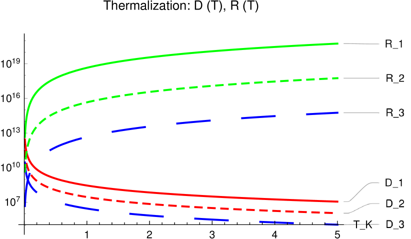
(a) Plots of the bulk and brane thermalization ratios $R(T),\ \Delta^{B}(T)$ versus temperature $T_{K}=T/m_{K}$ using $\hat{\lambda}_{3}=0.128,\ \hat{\lambda}^{B}_{3}=0.0225$ at fixed $\eta=1$ for three values $(1,10,100)$ of $g_{s}N\simeq 0.0836\times(z/\eta^{3})=(1,10,100)$ associated to $R_{1,2,3}(T)$ and $\Delta^{B}_{1,2,3}(T)$.

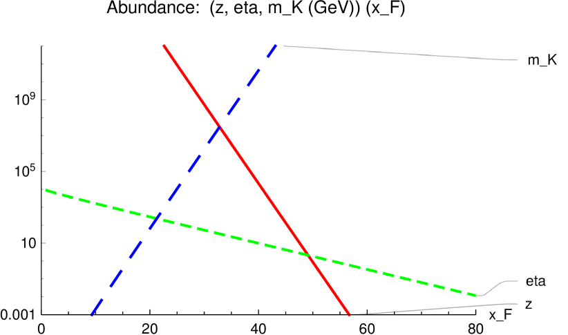
(b) Plots versus the freeze out variable $x_{F}=m_{K}/T_{K}$ of the solutions for $\eta,\ z$ and $m_{K}(GeV)$ reproducing the observed relic abundance $\Omega_{A}\simeq 0.11$.

Figure 5: Thermal equilibrium and cold thermal relic abundance constraints on the $A$-throat parameters $z,\ \eta$ at the warp factor value $w=w_{A}=10^{-4}$. The left panel $(a)$ displays the ratios to Hubble rate of the pair annihilation of bulk modes $R(T)$ and of the decay rates of bulk modes to pairs of brane modes $\Delta^{B}(T)$. The right (panel $(b)$) displays the admissible range of values for the parameters $z,\ \eta$ and the relic particle mass $m_{K}$ in GeV units.

We now wish to check whether some fraction of metastable ground state modes could survive as a cold thermal relic. For this purpose, we examine the conclusions implied by the freeze out mechanism based on the boundary-layer approach bender12 . The non-relativistic modes decoupling at $T/m_{K}>1$ is described by the familiar kinetic equation

$${dY(x)\over dx}=-\lambda x^{-n-2}(Y^{2}(x)-Y^{2}_{eq}(x)),\ [x={m_{K}\over T},\ Y(x)={n_{K}(t)\over T^{3}},\ Y_{eq}(x)=a\int_{0}^{\infty}ds{s^{2}\over e^{(s^{2}+x^{2})^{1/2}}\pm 1},$$ (V.8)

$$a\simeq 0.145g_{K}/g_{\star},\ g_{K}=5,\ \lambda=({90\over g_{\star}\pi^{2}})^{1/2}M_{\star}m_{K}<\sigma_{2\to 2}v>=({90\over g_{\star}\pi^{2}})^{1/2}{\xi^{4}\hat{\lambda}_{3}^{4}\over x_{m}^{3}}{\eta^{12}\over z^{3}w}]$$ (V.9)

where the annihilation rate has been set to $<\sigma_{2\to 2}v>=\sigma_{0}x^{-n},$ with $n\geq 0$ denoting the orbital momentum for the leading partial wave amplitude. For $s$-wave annihilation, $<\sigma_{2\to 2}v>=\lambda_{3}^{4}m_{K}^{2}=\xi^{2}(\eta^{3}/(M_{\star}w))^{4}\hat{\lambda}_{3}^{4}m_{K}^{2}$. The boundary-layer solution bender12 is derived by solving the equation analytically in two distinguished limits: one near the thermal equilibrium regime, $Y\simeq Y^{eq}$, in terms of the asymptotic series in the rate parameter $1/\lambda$, and the other in the post freeze out regime at large $x$ and small $Y^{eq}$. (In the alternative method presented in the textbook weinbergs08 , which we adopted in our previous work chemtob16 , $\lambda$ is denoted $B_{W}$.) The interval of $x$ near the freeze out point $x_{F}=m_{K}/T_{F}$, where the asymptotic series in $1/\lambda$ breaks down, is defined by the implicit equation for $x_{F}$,

$$x_{F}\simeq\ln(2a\lambda)-(n+{1\over 2})\ln x_{F},\ [a=0.145g_{K}/g_{\star}]$$ (V.10)

which relates $\lambda$ to $x_{F}$. The boundary-layer line interval around $x_{F}$ delimits the region where the solution for $Y(x)$ features a fast variation between the two regimes. The unknown parameters are determined by matching the analytic solution in this $x$-interval to the solutions (in the appropriate limits) in the outer intervals. The inner solution in the post freeze out limit, $T\to 0$, is then given by $Y(\infty)\simeq{(n+1)x_{F}^{2}\over\lambda(n+1+x_{F})}$, where $n=0$ for the $s$-wave annihilation case at hand. The present day abundance can then be evaluated from the formula

$$\Omega_{A}={T_{\gamma,0}^{3}\over 3M_{\star}^{2}H_{0}^{2}}{4\over 11}2m_{K}Y(\infty)={8T^{3}_{\gamma,0}\over 33H_{0}^{2}M_{\star}}({g_{\star}\pi^{2}\over 90})^{1/2}{w^{2}z^{2}\over\eta^{12}x_{m}^{2}\xi^{4}\hat{\lambda}_{3}^{4}}{x_{F}^{2}\over x_{F}+1},$$ (V.11)

where $H_{0}=1.44\ 10^{-42}GeV,\ T_{\gamma 0}=2.34\ 10^{-13}\ GeV,\ \Omega_{A}\simeq 0.11$. We consider at this point the interesting possibility that the parameters $z,\ \eta$ could be evaluated by solving the pair of cold relic constraint and abundance equations in Eqs. (V.10) and (V.11), which we rewrite in the more convenient forms

$${\eta^{4}\over z}=({e^{x_{F}}x_{F}^{1/2}w\over 2A^{\prime}})^{1/3},\ \Omega_{A}={Aw^{2}\over M_{\star}}({z\over\eta^{6}})^{2}{x_{F}^{2}\over x_{F}+1},$$ (V.12)

$$[A={8T_{\gamma,0}^{3}\over 33H_{0}^{2}}({g_{\star}\pi^{2}\over 90})^{1/2}{1\over x_{m}^{2}\hat{\lambda}_{3}^{4}\xi^{4}}\simeq 0.49\ 10^{7}{M_{\star}\over\hat{\lambda}_{3}^{4}},\ A^{\prime}=a({90\over g_{\star}\pi^{2}})^{1/2}{\xi^{4}\hat{\lambda}_{3}^{4}x_{m}^{3}}\simeq 0.38\ 10^{20}\hat{\lambda}_{3}^{4}].$$ (V.13)

The resulting solutions for the parameters $\eta$ and $z$ are given as a function of $x_{F}$ by

$$\eta=({A\over M_{\star}\Omega_{A}})^{1/4}({2A^{\prime}\over e^{x_{F}}x_{F}^{1/2}})^{1/6}w^{1/3}\simeq{1.17\ 10^{4.92}w^{1/3}\over(\hat{\lambda}_{3}\Omega_{A}^{1/2}(e^{x_{F}}\sqrt{x_{F}})^{1/3})^{1/2}},$$ (V.14)

$$z=\eta^{4}({2A^{\prime}\over e^{x_{F}}x_{F}^{1/2}w})^{1/3}={A\over M_{\star}\Omega_{A}}{2A^{\prime}\over e^{x_{F}}x_{F}^{1/2}}w\simeq{3.7\ 10^{26}w\over\Omega_{A}e^{x_{F}}\sqrt{x_{F}}},$$ (V.15)

where we have set for simplicity, $x_{F}^{2}/(x_{F}+1)\to x_{F}$ in $\Omega_{A}$. The proportionality relation $z\propto w$ satisfied by the solution implies that the predicted mass for the relic particle, $m_{K}=x_{m}wM_{\star}/z$, is warp factor independent. (The proportionality $\eta\propto w^{1/3}$ is compatible with the relation, $\eta^{3}/z\sim 1/(Ng_{s})$.) It is useful to compare the present result for $\Omega_{A}$ with that derived within the Chen-Tye approach chen06 , where the pair annihilation rate is set by the $2\to 1$ (instead of the $2\to 2$) process. With the reaction rate, $\Delta\Gamma_{2\to 1}=n_{K}(T)\sigma_{2\to 1}\sim\lambda_{3}^{2}T^{3}$, one finds that the resulting abundance at the radiation domination to matter domination (RDMD) time, $\Omega_{A}^{I}=2w^{2}M_{\star}/(g_{\star}^{1/4}(\xi\hat{\lambda}_{3})^{2}\rho_{RDMD})\simeq 2.5\ 10^{23}w^{2}/\eta^{6}$, is orders of magnitude larger (with our input parameters) than the present prediction in Eq. (V.13).

The solutions for $\eta,\ z$ obtained in our approximate solution to Boltzmann equation for the warped modes abundance are plotted in Fig. 5 as a function of the freeze out temperature for values in the interval $x_{F}=T_{F}/m_{K}\in(1,80)$. The selected values cover wide ranges owing to the exponential dependence on $x_{F}$. Settling on natural values for the $z,\ \eta$ parameters of $O(10)$, favours $x_{F}=T_{F}/m_{K}\sim 50$ with relic masses $m_{K}\sim 10^{12}$ GeV. Going down to $x_{F}=40$, selects larger parameters $\eta\sim 10,\ z\sim 10^{5}$ and a reduced mass $m_{K}\sim 10^{9}$ GeV, while allowing masses as small as $m_{K}\sim 100$ GeV, for $x_{F}=20$ and $\eta\sim 10^{2}$ requires the unrealistically large parameter value $z\sim 10^{15}$.

V.3 Double throat case

Since compactifications with multiple throats are not excluded, we here consider the case involving an additional $S$-throat of warp factor $w=w_{S}\sim 10^{-14}$ hosting TeV scale Standard Model $D3$-branes. The parameters $w,\ \eta,\ z$ defined in Subsection III.3 are now attached suffix labels $A,\ S$. Thermalization in the $S$-throat is accomplished by the fraction of warped modes tunneling from the $A$-throat. We shall consider the tunneling rate described by the $D3$-brane model in the resonant bulk case chen06 , $\Delta\Gamma_{tun}(A\to bulk)\approx\Delta\Gamma_{tun}(A\to S)\simeq w_{A}^{9}/{\cal R}_{A}$. (The non-resonant bulk case gives a much smaller rate, $\Delta\Gamma_{tun}(A\to S)\simeq w_{A}^{17}/{\cal R}_{A}$.) Recall that $A\to S$ tunneling takes place provided its rate exceeds the decay rate, $H^{-1}(t_{tun})\sim t_{tun}<\Delta t_{1\to 2}$, and that inverse tunneling from long to short throats is suppressed. Until tunneling terminates at time $t_{tun}\sim w_{A}^{-9}{\cal R}_{A}$, the cosmic bath is stuck in a matter dominated (MD) regime with the cosmic evolution satisfying the scaling laws, $T\propto a^{-2}\propto t^{-4/3},\ H=2/(3t),\ \rho=M_{\star}^{2}/t^{2}$.

The level matching condition, necessary for the tunneling from $A\to S$ throat to take place, requires that the modes level spacing be small compared to the tunneling width, $\delta m_{K}\simeq w_{S}/{\cal R}_{S}<\Gamma_{tun}\simeq w_{A}^{9}/{\cal R}_{A}$. This gives the upper bound $w_{S}\leq w_{A}^{9}{\cal R}_{S}/{\cal R}_{A}\simeq w_{A}^{9}(N_{S}/N_{A})^{1/4}$, favouring tunneling to longer throats chen06 . For $w_{S}<<w_{A}$, the low-lying $A$-throat modes change after tunneling to highly excited $S$-throat modes. Another constraint stems from the condition that the back-reaction from inflation in the $A$-throat does not produce closed strings in the $S$-throat. This is expressed by the bound on Hubble rate frey05 ; chen06 , $H^{4}(t)<N_{S}\tau_{3}w_{S}^{4}\sim N_{S}^{2}w_{S}^{4}/{\cal R}_{S}^{4}$, which imposes a minimal value for the warp factor, $w_{S}>H(t){\cal R}_{S}/N_{S}^{1/2}={H(t)\over M_{\star}}\eta_{S}^{3/2}z_{S}^{1/2}$ (where we used $N_{S}^{1/2}\simeq{\cal R}_{S}^{2}m_{s}^{2}\simeq z_{S}^{1/2}/\eta_{S}^{3/2}$). Setting the Hubble rate value at inflation exit $H(t_{I})\simeq 10^{-4}M_{\star}$ or at tunneling time $H(t_{tun})\simeq\Gamma_{tun}$, gives the lower bounds, $w_{S}>10^{-4}\eta_{S}^{3/2}z_{S}^{1/2}$ or $w_{S}>w_{A}^{9}\eta_{S}^{3/2}z_{S}^{1/2}/z_{A}$.

One can use the time-temperature and energy-temperature relations, ${1\over 2t}\equiv H=0.33g_{\star}^{1/2}(T){T^{2}\over M_{\star}},\ \rho(T)\equiv 3M_{\star}^{2}H^{2}={\pi^{2}\over 30}g_{\star}(T)T^{4},\ [g_{\star}(T)=({T\over\alpha})^{\gamma},\ \alpha={w\over{\cal R}}]$ to obtain the temperature at tunneling time in a generic throat $X$, $T_{X}(t_{tun})=(({M_{\star}\Gamma_{tun}/0.66})^{2}\alpha_{X}^{\gamma})^{1/(4+\gamma)}$. Adapting this result to the $A$- and $S$-throats with $\gamma=5$ gives the temperatures

$${T_{S}(t_{tun})\over GeV}=2.67\ 10^{18}w_{A}^{2}({w_{S}^{5}\over z_{A}^{2}z_{S}^{5}})^{1/9},\ {T_{A}(t_{tun})\over GeV}=2.67\ 10^{18}{w_{A}^{23/9}\over z_{A}^{7/9}}.$$ (V.16)

The wide gap between the respective warp factors entails that $T_{S}<<T_{A}$. The thermal equilibrium condition at tunneling time can be described for simplicity by forming the ratio of the $2\to 1$ annihilation rate to Hubble rate, $R_{X}(t_{tun})={\Delta\Gamma_{2\to 1}/H(t_{tun})}$, where $\Delta\Gamma_{2\to 1}=n(t)\sigma_{2\to 1}\simeq\alpha^{-\gamma}T_{tun}^{3+\gamma}\lambda_{3}^{2}\simeq\alpha_{X}^{-\gamma/(\gamma+4)}({M_{\star}\Gamma_{tun}/0.66})^{2(\gamma+3)/(\gamma+4)}$. Adapting the general formula

$$R_{X}(t_{tun})={(\xi\hat{\lambda}_{3})^{2}\ \eta_{X}^{6}\over(0.66)^{2(\gamma+3)/(\gamma+4)}}{z_{X}^{\gamma/(\gamma+4)}\over w_{X}^{(3\gamma+8)/(\gamma+4)}(M_{\star}t_{tun})^{(\gamma+2)/(\gamma+4)}},$$ (V.17)

to the $A$- and $S$-throats, gives $R_{S}(t_{tun})=1.82\ 10^{8}\eta_{S}^{6}{z_{S}^{5/9}w_{A}^{7}/(z_{A}^{7/9}w_{S}^{23/9})},\ R_{A}(t_{tun})=1.82\ 10^{8}\eta_{A}^{6}{w_{A}^{40/9}/z_{A}^{2/9}},$ where we used the inputs values $\gamma=5,\ \xi=7.3\ 10^{4},\hat{\lambda}_{3}=0.128,\ x_{m}=3.83$. We see that both ratios lie comfortably above unity and that thermalization sets in more rapidly in the $S$-throat.

In order to avoid disrupting the primordial abundance of light nuclei the universe temperature at tunneling time must lie above the nucleosynthesis threshold. Imposing the condition $T_{S,A}(t_{tun})>O(1)\ MeV$ in Eqs. (V.16) yields the lower bounds on warp factors, $w_{S}>10^{-117/5}z_{A}^{2/5}z_{S}$ and $w_{A}>10^{-189/23}z_{A}^{7/23}.$ A useful constraint also arises chen06 by substituting the above condition $\Gamma_{tun}=H_{tun}\leq w_{S}N_{S}^{1/2}/{\cal R}_{S}\simeq w_{S}{\cal R}_{S}m_{s}^{2}$ into Eq. (V.16). The resulting upper bound on the $S$-throat temperature, $T_{S}(t_{tun})=((w_{S}/{\cal R}_{S})^{\gamma}(M_{\star}\Gamma_{tun})^{2})^{1/(\gamma+4)}<(w_{S}^{\gamma+2}z_{S}^{(2-\gamma/4)}\eta_{S}^{3\gamma/4})^{1/(\gamma+4)}m_{s}$, lies below the warped mass mass $w_{A}/{\cal R}_{A}$ (upon replacing $m_{s}\to N_{A}^{1/4}/{\cal R}_{A}$) but could dangerously exceed the warped string mass scale $w_{S}m_{s}$ unless one invokes some fine tuning of the parameters.

We consider next the cold thermal relic abundance using the above $2\to 1$ pair annihilation rate as in Chen-Tye approach chen06 . In this description, the relationship $t\simeq 1/(2H(t))=M_{\star}/(0.66\ g_{\star}^{1/2}T^{2})$ sets the decoupling time when modes become non-relativistic ($T_{NR}\simeq m_{K}$) at $t_{NR}\simeq M_{\star}/(0.66\alpha_{A}^{2}x_{m}^{(4+\gamma)/2})$. The modes abundance at decoupling in the $A$-throat, $\rho_{K}/m_{K}^{4}=n_{K}(t_{NR})/m_{K}^{3}$, is set by substituting the modes number density, $n_{K}(t)\equiv H(t)/D\Gamma_{ann}=1/(2t\lambda_{3}^{2})$, and inserting the softening factor $(t_{tun}/t_{NR})^{-1/2}$ to account for the extended matter domination period in the $A$-throat until tunneling is completed. The resulting general formula for the cold relic abundance, $\Omega_{X}^{II}={1\over(0.33\ 3^{1.5})^{1/2}x_{m}^{\gamma/4}}{M_{\star}\over\rho_{RDMD}^{1/4}}({t_{NR}\over t_{tun}})^{1/2}{w^{2}_{X}\over(\xi\hat{\lambda}_{3})^{2}\eta_{X}^{6}}$, yields the abundance in the $A$- and $S$-throats

$$\Omega_{S}^{II}=2.38\ 10^{17}{w_{S}w_{A}^{9/2}z_{S}\over\eta_{S}^{6}z_{A}^{1/2}},\ \ \Omega_{A}^{II}=2.38\ 10^{17}{w_{A}^{11/2}z_{A}^{1/2}\over\eta_{A}^{6}}.$$ (V.18)

It is clear that the $A$-throat contribution to the abundance is largely dominant. Note that the present prediction using our input parameters is considerably suppressed relative to Chen-Tye estimate chen06 $\Omega_{A}^{II}\simeq 10^{24}w_{A}^{11/2}z_{A}^{1/2}\eta_{A}^{-6}$, which is helpful in relaxing the bounds on parameters.

VI Summary and main conclusions

We discussed in this work Kaluza-Klein theory for type $II\ b$ supergravity on Klebanov-Strassler background based on a large radial distance approximation that preserves the non-singular geometry near the conifold apex. The WKB method was used to obtain predictions for masses, wave functions and interactions of warped graviton, axio-dilaton and scalar (4-form) modes. The most robust results are for graviton modes. The mass splittings for radial, orbital and string excitations cluster around $1\ -\ 1.5$ in units $g_{s}M\epsilon^{2/3}/m_{s}^{2}$. In comparison to graviton modes, the dilaton modes are slightly heavier, due to the 3-fluxes contributions, while the non-singlet scalar modes are significantly lighter, due to attractive contributions from mixing the 4-form and internal metric supergravity fields. The possibility that the scalar mode $S_{-}(100)$ be a natural candidate for the LCKP berndsen07 is mitigated by the substantial mixings between scalar modes of diverse origins in the classical background anticipated from studies of mass spectra for multidimensional field spaces berg06 ; benna07 . The background deformations from compactification effects have a strong impact on the interactions of warped modes, modifying the selection rules imposed by the throat isometry and imposing large hierarchies on decay rates of lightest modes freydacline09 . The sensitivity of warped modes couplings to the infrared geometry is made manifest by strongly suppressed value for the effective gravitational mass scale $\Lambda_{KK}\simeq M_{\star}/\Phi_{n}(r_{0})$ relative to the estimates in models using softened warp profiles.

The thermal evolution of a cosmic component of warped Kaluza-Klein modes produced in the throat hosting $D3-\bar{D}3$-brane inflation provides useful constraints on the compactification and warped throat dimensionless parameters $\eta=L_{W}/{\cal R},\ z=M_{\star}{\cal R}$ and $w$. We pursued an analysis along same lines as chen06 using updated values for the pair annihilation and two-body decay reactions of warped modes. Both the initial temperature from branes annihilation or the reheat temperature from decays of massive closed strings lie well below the warped string theory mass scale. The throat and brane thermalizations take easily place at temperatures of same orders as the lightest warped modes. The empirical value for the cold thermal relic abundance can be reproduced in a wide interval of the warped modes mass including the TeV range, but a robust conclusion would require a quantitative analysis of Boltzmann equation.

Appendix A Review of warped deformed conifold

We provide in this appendix an introductory review on the deformed conifold. After a summary of algebraic and differential geometry properties we discuss the harmonic analysis witin the group theory approach of pufu10 . We consider next the modified Klebanov-Strassler solution for the metric tensor replacing the conifold base $T^{1,1}$ by the direct product manifold of geometry $S^{2}\times S^{3}$ firouz06 and finally describe a simple construct that makes contact with the analytic type formalism in the singular conifold limit.

A.1 Algebraic properties

The deformed conifold ${\cal C}_{6}$ candelas90 is part of the family of Stenzel spaces ${\cal C}_{2d-2}$ cveticpope00 , defined as non-compact manifolds of complex dimension $(d-1)$ satisfying the quadratic embedding equation in $C^{d}$,

$$\sum_{a=1}^{d}w_{a}^{2}=\epsilon^{2},\ [\epsilon\in R,\ w_{a}\in C]$$ (A.1)

where $\epsilon\in C$ is the complex structure deformation modulus. The invariance under $SO(d)$ orthogonal matrix rotations of the complex variables $w_{a},\ [a=1,\cdots,d]$ entails the existence of the isometry group $G=SO(d)\times Z_{2}^{R}$. At $\epsilon=0$, the $Z_{2}^{R}$ parity $w_{a}\to-w_{a}$ is promoted to the conserved charge $U(1)_{R}:\ w_{a}\to e^{i\alpha}w_{a}$, where the suffix label for $U(1)_{R}$ is a reminder that this corresponds to the R-symmetry of the 4-d ${\cal N}=1$ supersymmetric dual gauge theory. The radial sections $\Sigma_{\tau}$ at constant $\tau$ lie at the intersections of the conifold $\sum_{a}w_{a}^{2}=\epsilon^{2}$ with the locus $\sum_{a}|w_{a}|^{2}=|\epsilon|^{2}\cosh\tau$. The fact that the undeformed Stenzel spaces (at $\epsilon=0$) are real cones over a compact base manifold suggests the convenient parameterization of the $w_{a}$ at finite $\epsilon$ combining the real radial variable $\tau\in[0,\infty]$ with the $d$ pairs of complex conjugate variables $y_{a},\ \bar{y}_{a}$ parameterizing the $\Sigma_{\tau}$ satifying the two conditions

$$\sum_{a}y_{a}^{2}=0,\ \sum_{a}|y_{a}|^{2}=1,\ \ [w_{a}={\epsilon\over\sqrt{2}}(e^{\tau/2}y_{a}+e^{-\tau/2}\bar{y}_{a})\ \Longrightarrow\ y_{a}={e^{\tau/2}w_{a}/\epsilon-e^{-\tau/2}(w_{a}/\epsilon)^{\star}\over\sqrt{2}\sinh\tau}].$$ (A.2)

The radial sections are compact manifolds homeomorphic to Stiefel coset spaces $V_{d,2}=SO(d)/SO(d-2)$ whose elements are organized into equivalence classes $g\sim gh,\ [g\in SO(d),\ h\in SO(d-2)]$ corresponding to orbits of the isometry group $SO(d)$ acting on the element $y^{(0)}_{a}=(0,0,\cdots,i\sinh(\tau/2),\cosh(\tau/2))$ fixed under the stabilizer group $SO(d-2)$. Near $\tau=0,\ y^{(0)}_{a}=(0,0,\cdots,0,1)$ and $\Sigma_{\tau}\sim SO(d)/SO(d-1)\sim S^{d-1}$. Since the $\Sigma_{\tau}\sim V_{d,2}$ have the same integration measure $\mu_{SO(d)}/\mu_{SO(d-2)}$ up to an overall $\tau$-dependent normalization, the representation vector space for the group $SO(d)$ action on $\Sigma_{\tau}$ consists of square normalizable functions with the integration measure given by the group $G$ invariant measure times a function of $\tau$.

The spaces ${\cal C}_{2d-2}$ are Kähler manifolds equipped with a Hermitean metric generated by the isotropic Kähler potential ${\cal F}(\tau)$,

$$d\tilde{s}^{2}({{\cal C}_{2d-2}})=g_{a\bar{b}}dw^{a}d\bar{w}^{\bar{b}},\ [g_{a\bar{b}}={\partial^{2}{\cal F}\over\partial w_{a}\partial\bar{w}_{\bar{b}}}=2F_{1}\delta_{ab}+4F_{2}\bar{w}_{a}w_{b}={{\cal F}^{\prime}\over\epsilon^{2}\sinh\tau}\delta_{ab}+{{\cal F}^{\prime\prime}-{\cal F}^{\prime}\coth\tau\over\epsilon^{4}\sinh^{2}\tau}\bar{w}_{a}w_{b}].$$ (A.3)

The Ricci tensor flatness condition (on Calabi-Yau manifolds), $R_{a\bar{b}}=0$, imposes a differential equation on ${\cal F}^{\prime}(\tau)=\partial_{\tau}{\cal F}(\tau)$ which can be solved in terms of Hypergeometric functions pufu10 ; cveticpope00

$$({{\cal F}^{\prime}(\tau)\over\epsilon^{2}\sinh\tau})^{d-2}{\cal F}^{\prime\prime}={d-2\over d-1}\ \Longrightarrow\ {\cal F}^{\prime}(\tau)=\epsilon^{4\over d-1}R^{1\over d-1}(\tau),$$ (A.4)

$$[R(\tau)={d-2\over\epsilon^{2}}\int_{0}^{\tau}dv(\sinh(v))^{d-2}={(d-2)\over\epsilon^{2}(d-1)}(2\sinh(\tau/2))^{d-1}{{}_{2}}F_{1}({d-1\over 2},{3-d\over 2};{d+1\over 2};-\sinh^{2}(\tau/2))].$$ (A.5)

We specialize hereafter to the conifold case ($d=4$) where the complex variables $w_{a},\ [a=1,\cdots,4]$ and their linear combinations $z_{a}$, can be conveniently packaged within the $2\times 2$ matrix $W$ which allows defining the conifold and its fixed-$\tau$ sections $\Sigma_{\tau}$ by the pair of algebraic equations

$$Det\ (W)=-\sum_{a}w_{a}^{2}=z_{1}z_{2}-z_{3}z_{4}=-\epsilon^{2},\ {1\over 2}Tr(W^{\dagger}W)=\sum_{a}|w_{a}|^{2}=\sum_{a}|z_{a}|^{2}=\hat{r}^{3}=({2\over 3})^{3/2}r^{3}=|\epsilon|^{2}\cosh\tau,$$ (A.6)

$$[W=\pmatrix{w^{3}+iw^{4}&w^{1}-iw^{2}\cr w^{1}+iw^{2}&-w^{3}+iw^{4}}\equiv\pmatrix{z_{3}&z_{1}\cr z_{2}&z_{4}},\ {w_{1}\choose-iw_{2}}={1\over 2}(z_{1}\pm z_{2}),\ {w_{3}\choose iw_{4}}={1\over 2}(z_{3}\mp z_{4})].$$ (A.7)

(Our normalization conventions for $w_{a}$ and $W$ coincide with krishtein08 ; benini09 and would agree with gimon02 if one substitutes $w_{a}\to\sqrt{2}w_{a},\ W\to\sqrt{2}W$.) The metric tensor can be evaluated by means of the formula

$$d\tilde{s}^{2}({{\cal C}_{6}})={1\over 2}{\partial{\cal F}\over\partial\hat{r}^{3}}Tr(dW^{\dagger}dW)+{1\over 4}{\partial^{2}{\cal F}\over\partial(\hat{r}^{3})^{2}}]|Tr(W^{\dagger}dW)|^{2}=(2F_{1}\delta_{ab}+4F_{2}\bar{w}_{a}w_{b})dw^{a}\bar{d}w^{b},$$ (A.8)

$$[F_{1}\equiv{1\over 2}{\partial{\cal F}\over\partial\hat{\rho}^{2}}={\epsilon^{-2/3}K(\tau)\over 2},\ F_{2}\equiv{1\over 4}{\partial^{2}{\cal F}\over\partial(\hat{\rho}^{2})^{2}}={\epsilon^{-8/3}K^{\prime}(\tau)\over 4\sinh\tau}\equiv{\epsilon^{-8/3}K(\tau)\over 4\sinh^{2}\tau}({2\over 3K^{3}(\tau)}-\cosh\tau)]$$ (A.9)

where $\epsilon^{2}\sinh\tau d\tau=w_{a}d\bar{w}_{a}+\bar{w}_{a}dw_{a}$ and

$${\cal F}^{\prime}(\tau)\equiv{\partial{\cal F}\over\partial\tau}=\epsilon^{4/3}(\sinh(\tau)\cosh(\tau)-\tau)^{1/3}=\epsilon^{4/3}\sinh(\tau)K(\tau),\ {\cal F}^{\prime\prime}\equiv{\partial^{2}{\cal F}\over\partial\tau^{2}}={2\over 3}({\epsilon^{2}\sinh\tau\over{\cal F}^{\prime}})^{2}.$$ (A.10)

At large $\tau$, the above metric is asymptotic to the undeformed conifold metric,

$$ds^{2}({\cal C}_{6})\simeq dr^{2}+r^{2}ds^{2}(V_{4,2}),\ [r^{2}\equiv{3\over 2}\hat{r}^{2}={3\over 2^{5/3}}\epsilon^{4/3}e^{2\tau/3}]$$ (A.11)

where the sections at fixed values of the conic radial variable $r$ have the coset space structure $\Sigma_{\tau}=SU(2)_{1}\times SU(2)_{2}/U(1)_{H}\sim T^{1,1}$. The invariance of the embedding equations in Eq.(A.7) under $SO(4)$ rotations of the $w_{a}$, modulo the $Z_{2}^{R}$-parity $w_{a}\to-w_{a}$, follows from the determinant and trace invariance under left and right multiplication by unitary matrices, $W\to g_{1}Wg_{2}^{\dagger},\ [g_{i}\in SU(2)_{i},\ i=1,2]$, modulo $W\to-W$. The Klebanov-Strassler standard solution for the metric klebstrass00 in Eq. (II.20) follows from the parameterization of $W$ minasian99

$$W=g_{1}W_{\epsilon}\sigma_{3}\sigma_{1}g_{2}^{\dagger}={\epsilon}g_{1}e^{\tau\sigma_{3}/2}\sigma_{1}g_{2}^{\dagger}={\epsilon}g_{1}\pmatrix{0&e^{\tau/2}\cr e^{-\tau/2}&0}g_{2}^{\dagger},\ [W_{\epsilon}=\epsilon\pmatrix{e^{\tau/2}&0\cr 0&-e^{-\tau/2}},$$ (A.12)

$$g_{i}=e^{+i{\phi_{i}\over 2}\sigma_{3}}e^{-i{\theta_{i}\over 2}\sigma_{2}}e^{+i{\varphi_{i}\over 2}\sigma_{3}}=\pmatrix{c_{i}e^{i(\varphi_{i}+\phi_{i})/2}&-s_{i}e^{i(-\varphi_{i}+\phi_{i})/2}\cr s_{i}e^{-i(-\varphi_{i}+\phi_{i})/2}&c_{i}e^{-i(\varphi_{i}+\phi_{i})/2}},\ c_{i}=\cos{\theta_{i}\over 2},\ s_{i}=\sin{\theta_{i}\over 2}]$$ (A.13)

where the pair of Euler angles $(\theta_{i},\ \phi_{i},\ \varphi_{i})$ of $SU(2)_{i}\sim S^{3}_{i}$ are subject to the equivalence $\varphi_{1}=\varphi_{2}=\psi/2$.

The complex coordinates $y_{a}$ in Eq. (A.2) can be expressed as quadratic products of the two $2$-spinors $a=(a_{i})\in({1\over 2},0),\ b=(b_{i})\in(0,{1\over 2}),\ [i=1,2]$ of the isometry group $SU(2)_{1}\times SU(2)_{2}$ candelas90

$${y_{1}\choose-iy_{2}}={a_{1}b_{1}\mp a_{2}b_{2}\over\sqrt{2}},\ {y_{3}\choose iy_{4}}=-{a_{1}b_{2}\pm a_{2}b_{1}\over\sqrt{2}},\ [a_{(1,2)}={\cos{\theta_{1}\over 2}\choose\sin{\theta_{1}\over 2}}e^{{i\over 2}(\pm\phi_{1}+{\psi\over 2})},\ b_{(1,2)}={\cos{\theta_{2}\over 2}\choose\sin{\theta_{2}\over 2}}e^{{i\over 2}(\pm\phi_{2}+{\psi\over 2})}].$$ (A.14)

The $a_{i},\ b_{i}$ correspond in the Klebanov-Witten dual gauge theory klewit98 to the pair of chiral supermultiplet fields $A_{i},\ B_{i},\ [i=1,2]$ carrying the quantum numbers $A_{i}\sim(N_{1},\bar{N}_{2};2,1)_{{1\over 2},1},\ B_{i}\sim(\bar{N}_{1},N_{2};1,2)_{{1\over 2},-1}$ with respect to the gauge and global symmetry groups ${\cal G}=SU(N_{1})\times SU(N_{2})$ and $G=SU(2)_{1}\times SU(2)_{2}\times U(1)_{r}\times U(1)_{b}$. The complex variables $z_{a}$ in Eq. (A.7) correspond then to the gauge theory composite fields $M_{ij}=B_{i}A_{j}$ with $(z_{1},\ z_{2},\ z_{3},\ z_{4})\sim(B_{2}A_{1},\ B_{1}A_{2},\ B_{1}A_{1},\ B_{2}A_{2})$

The deformed conifold embedding in $C^{4}$ is conveniently defined by the parameterization of the four complex coordinates herzog01 ; mcguirk12 ,

$$w_{1}=\epsilon[\cosh{S}\cos\theta_{+}\cos\phi_{+}+i\sinh{S}\cos\theta_{-}\sin\phi_{+}],\ w_{2}=\epsilon[-\cosh{S}\cos\theta_{+}\sin\phi_{+}+i\sinh{S}\cos\theta_{-}\cos\phi_{+}],\$$ (A.15)

$$w_{3}=\epsilon[-\cosh{S}\sin\theta_{+}\cos\phi_{-}+i\sinh{S}\sin\theta_{-}\sin\phi_{-}],\ w_{4}=\epsilon[-\cosh{S}\sin\theta_{+}\sin\phi_{-}-i\sinh{S}\sin\theta_{-}\cos\phi_{-}],$$ (A.16)

$$[S={\tau+i\psi\over 2},\ \theta_{\pm}={1\over 2}(\theta_{1}\pm\theta_{2}),\ \phi_{\pm}={1\over 2}(\phi_{1}\pm\phi_{2})]$$ (A.17)

derived by substituting Eq.(A.14) into Eq.(A.2). Evaluating Eq. (A.9) in this parameterization yields the Klebanov-Strassler metric in Eq. (II.15), which we rewrite below for convenience,

$$d\tilde{s}^{2}({\cal C}_{6})={\epsilon^{4/3}K(\tau)\over 2}({1\over 3K^{3}(\tau)}(d\tau^{2}+(g^{(5)})^{2})+\cosh^{2}({\tau\over 2})((g^{(3)})^{2}+(g^{(4)})^{2})+\sinh^{2}({\tau\over 2})((g^{(1)})^{2}+(g^{(2)})^{2}),$$ (A.18)

$$[g^{(1,3)}={1\over\sqrt{2}}(e^{(1)}\mp e^{(3)}),\ g^{(2,4)}={1\over\sqrt{2}}(e^{(2)}\mp e^{(4)}),\ g^{(5)}=e^{(5)},$$ (A.19)

$${e^{(1)}\choose e^{(2)}}={-\sin\theta_{1}d\phi_{1}\choose d\theta_{1}},\ {e^{(3)}\choose e^{(4)}}=\pmatrix{\cos\psi&-\sin\psi\cr\sin\psi&\cos\psi}{\sin\theta_{2}d\phi_{2}\choose d\theta_{2}},\ e^{(5)}=d\psi+\sum_{i=1}^{2}\cos\theta_{i}d\phi_{i}]$$ (A.20)

where $e^{(a)}$ and $g^{(a)}$ are two bases of left invariant 1-forms of the compact base whose volume form integral yields the base manifold volume

$$V(T^{1,1})={1\over\sqrt{9\cdot 6^{4}}}\int g^{(1)}\wedge\cdots\wedge g^{(5)}={1\over 108}\int_{0}^{\pi}\sin\theta_{1}\int_{0}^{\pi}\sin\theta_{2}\int_{0}^{2\pi}d\phi_{1}\int_{0}^{2\pi}d\phi_{2}\int_{0}^{4\pi}d\psi={16\pi^{3}\over 27}].$$ (A.21)

An alternative formula for the metric kuperstein04 ; kupsonn08 is sometimes used in terms of the bases of left invariant 1-forms $h_{a},\ \tilde{h}_{a},\ [a=1,2,3]$ associated to the Lie algebra generators $g_{1}^{\dagger}dg_{1}={i\over 2}h_{a}\sigma_{a},\ g_{2}^{\dagger}dg_{2}={i\over 2}\tilde{h}_{a}\sigma_{a}$ of the $SU(2)_{a}$ groups, $g_{a}=e^{+i{\phi_{i}\over 2}\sigma_{3}}e^{-i{\theta_{i}\over 2}\sigma_{2}}e^{+i{\psi\over 4}\sigma_{3}},\ [a=i=1,2]$. The 1-forms $h_{a},\ \tilde{h}_{a}$ satisfy the $SU(2)$ Maurer-Cartan relations, $dh_{a}={i\over 2}\epsilon_{abc}h_{b}\wedge h_{c},\ d\tilde{h}_{a}={i\over 2}\epsilon_{abc}\tilde{h}_{b}\wedge\tilde{h}_{c}$ and are related to the basis $g^{(a)}$ in Eq. (A.20) by the 2-d rotations,

$${h_{1}\choose h_{2}}={1\over\sqrt{2}}{\cal R}_{\psi/2}{g^{(1)}+g^{(3)}\choose g^{(2)}+g^{(4)}},\ {\tilde{h}_{1}\choose\tilde{h}_{2}}={1\over\sqrt{2}}{\cal R}^{\prime}_{\psi/2}{g^{(3)}-g^{(1)}\choose g^{(4)}-g^{(2)}},\ h_{3}+\tilde{h}_{3}=g^{(5)},$$ (A.22)

$$[{\cal R}_{\psi/2}=\pmatrix{\cos{\psi\over 2}&\sin{\psi\over 2}\cr\sin{\psi\over 2}&-\cos{\psi\over 2}},\ {\cal R}^{\prime}_{\psi/2}=\pmatrix{-\cos{\psi\over 2}&-\sin{\psi\over 2}\cr\sin{\psi\over 2}&-\cos{\psi\over 2}},$$ (A.23)

and to the basis $(e_{1,2},\ \epsilon_{1,2,3})$ of papado00 as, $h_{1,2}=e_{1,2},\ \tilde{h}_{1,2}=\epsilon_{1,2},\ (h_{3}+\tilde{h}_{3})=\epsilon_{3}.$ Note that $h_{1}^{2}=(g^{(1)}+g^{(3)})^{2},\ h_{2}^{2}=(g^{(2)}+g^{(4)})^{2},\ \tilde{h}_{1}^{2}=(g^{(1)}-g^{(3)})^{2},\ \tilde{h}_{2}^{2}=(g^{(2)}-g^{(4)})^{2}$. Substitution in Eq. (A.20) leads to the alternative equivalent expression for the Klebanov-Strassler metric solution kuperstein04 ,

$$d\tilde{s}^{2}({{\cal C}_{6}})=\epsilon^{4/3}[B^{2}(\tau)(d\tau^{2}+(h_{3}+\tilde{h}_{3})^{2})+A^{2}(\tau)(h_{1}^{2}+h_{2}^{2}+\tilde{h}_{1}^{2}+\tilde{h}_{2}^{2}+{2\over\cosh\tau}(h_{2}\tilde{h}_{2}-h_{1}\tilde{h}_{1}))],$$ (A.24)

$$[A^{2}(\tau)=2^{-7/3}\coth\tau(\sinh 2\tau-2\tau)^{1/3}={1\over 4}\cosh\tau K(\tau)={{\cal F}^{\prime}(\tau)\over 4e^{4/3}A^{2}(\tau)\tanh\tau},$$ (A.25)

$$B^{2}(\tau)=2^{-1/3}3^{-1}\sinh^{2}\tau(\sinh 2\tau-2\tau)^{-2/3}={1\over 6K^{2}(\tau)}].$$ (A.26)

Another useful parameterization of the deformed conifold metric gimon02 is obtained by representing the matrix $W$ by the product of $2\times 2$ unitary matrices $S\in{SU(2)\over U(1)}\sim S^{2},\ T\in SU(2)\sim S^{3}$, associated to the collapsing 2-sphere and the blown-up 3-sphere near the apex, of angle coordinates $\theta,\phi$ and $(\theta_{2},\phi_{2},\psi)\sim\omega_{a}$,

$${1\over\sqrt{2}}W=iXP\equiv{\epsilon}TSe^{\tau\sigma_{3}\over 2}S^{\dagger}\sigma_{3},\ [X=-iT\sigma_{3},\ P={\epsilon}U\pmatrix{e^{\tau/2}&0\cr 0&e^{-\tau/2}}U^{\dagger},\ U=\sigma_{3}S\sigma_{3},$$ (A.27)

$$S=e^{i\phi\sigma_{3}/2}e^{-i\theta\sigma_{1}/2},\ S^{\dagger}dS={i\over 2}s^{a}\sigma_{a}={i\over 2}(-d\theta\sigma_{1}+\sin\theta d\phi\sigma_{2}+\cos\theta d\phi\sigma_{3}),\ T^{\dagger}dT={i\over 2}\omega^{a}\sigma_{a},\ [a=1,2,3]].$$ (A.28)

The resulting expression of the metric solution is given by

$$d\tilde{s}^{2}({\cal C}_{6})={\epsilon^{4/3}\over 6K^{2}(\tau)}(d\tau^{2}+H_{3}^{2})+{\epsilon^{4/3}K(\tau)\over 4}[\cosh^{2}({\tau\over 2})(H_{1}^{2}+H_{2}^{2})+\sinh^{2}({\tau\over 2})((2d\theta+H_{2})^{2}+(2\sin\theta d\phi-H_{1})^{2})],$$ (A.29)

$$[\pmatrix{H_{1}\cr H_{2}\cr H_{3}}=\pmatrix{0&\cos\theta&-\sin\theta\cr 0&1&0\cr 0&\sin\theta&\cos\theta}\pmatrix{\sin\phi&\cos\phi&0\cr\cos\phi&-\sin\phi&0\cr 0&0&1}\pmatrix{\omega_{1}\cr\omega_{2}\cr\omega_{3}},\ \pmatrix{\omega_{1}\cr\omega_{2}\cr\omega_{3}}=-\pmatrix{\cos\psi d\theta_{2}+\sin\psi\sin\theta_{2}d\phi_{2}\cr-\sin\psi d\theta_{2}+\cos\psi\sin\theta_{2}d\phi_{2}\cr d\psi+\cos\theta_{2}d\phi_{2}}]$$ (A.30)

where we have displayed in the second line the rotations transforming $\omega_{a}\to H_{a}$, with ${\cal R}_{\theta}^{(i,j)},\ {\cal R}_{\phi}^{{}^{\prime}(i,j)}$ being $SO(3)$ representation matrices for $S$ associated to rotations in the planes $(i,j)$ of the space $R^{3}$ embedding $S^{2}(\theta,\phi)$. The bases of 1-forms $s_{a}$ and $\omega_{a}$ are related by $\omega^{a}S^{\dagger}\sigma_{a}S=(H_{1}\sigma_{1}-H_{2}\sigma_{2}+H_{3}\sigma_{3})\ \Longrightarrow\ H_{a}=({\cal R}_{\theta}^{(2,3)}\cdot{\cal R}_{\phi}^{(1,2)^{\prime}})_{ab}\omega_{b}.$ Identifying the expressions of $Tr(dW^{\dagger}dW),\ |Tr(W^{\dagger}dW)|^{2}$ in the parameterizations of $W$ in Eqs. (A.13) and (A.28) allows expressing the bases of 1-forms $g^{(a)}$ as linear combinations of the 1-forms $s_{1},\ s_{2}$ and $H_{a}$ ($S$-conjugates to the $\omega_{a}$),

$$(g^{(1)}+ig^{(2)})={e^{i\psi}\over\sqrt{2}}((H_{1}-2\sin\theta d\phi)+i(H_{2}+2d\theta)),\ (g^{(3)}+ig^{(4)})={e^{i\psi}\over\sqrt{2}}(H_{1}+iH_{2}),\ g^{(5)}=H_{3}.$$ (A.31)

The $\tau\to 0$ limit of the metric in Eq. (A.30),

$$d\tilde{s}^{2}({\cal C}_{6})\simeq{\epsilon^{4/3}\over 2^{5/3}3^{1/3}}(d\tau^{2}+\sum_{a=1}^{3}\omega_{a}^{2}+\tau^{2}((d\theta+{1\over 2}H_{2})^{2}+(\sin\theta d\phi-{1\over 2}H_{1})^{2}))$$ (A.32)

$$\Longrightarrow\ \tilde{r}(S^{3})=\tilde{r}(S^{2})/\tau=\epsilon^{2/3}2^{-5/6}3^{-1/6},\ [r^{2}(S^{3})=h^{1/2}(0)\tilde{r}^{2}(S^{3})=2^{-4/3}3^{-1/3}a_{0}^{1/2}g_{s}M\alpha^{\prime}]$$ (A.33)

shows that the geometry near the apex involves the collapsing $S^{2}(\theta,\phi)$ fibred over the blown-up $S^{3}(\omega^{a})$, where the formulas for the unwarped and warped radii $\tilde{r}(S^{k}),\ r(S^{k})$ were inferred by means of the familiar method minasian99 .

We observe in conclusion that the deformed conifold stands out as the prototype for conic Calabi-Yau threefolds realizing AdS/CFT string-gauge theory duality by quiver gauge theories with a renormalization group flow of Seiberg cascading type. Meanwhile, several families of 6-d conic Calabi-Yau throats with horizons given by Sasaki-Einstein bases and similar duality properties were discovered. One example is the infinite family of 5-d manifolds $Y^{p,q}$ of topology $S^{2}\times S^{3}$ providing horizons of conic Calabi-Yau manifolds labelled by relative prime integers $p,\ q$, which arise as partial toric resolutions of $C^{3}/(Z_{p}\times Z_{p})$ orbifolds. The string theory compactifications on the asymptotic $AdS_{5}\times Y^{p,q}$ spacetimes martelli04 are dual to superconformal quiver gauge theories benvsparks04 . The supergravity solution at large radial distances from the apex region is discussed in herzov04 . An iterative construction of the quiver gauge theories on $ND3$-brane probes is presented in benvenuti04 and the embedding of supersymmetry preserving flavour $Dp$-branes for $p=3,5,7$ is discussed in canoura05 .

A.2 Harmonic analysis

Harmonic analysis is the branch of mathematics dealing with the decomposition of smooth fields on manifolds using orthonormal bases of square integrable functions given by eigenfunctions of the manifolds Laplace-Beltrami operators. We here summarize the decomposition of scalar fields on harmonic functions of Stenzel spaces ${\cal C}_{2d-2}$ developed in pufu10 in terms of the constrained systems of coordinates $y_{a}$ for the radial sections $V_{d,2}=SO(d)/SO(d-2)$.

The wave functions in fixed representations of $SO(d)$ are given by linear combinations with $\tau$-dependent coefficients of homogeneous polynomials of the constrained systems of coordinates $y_{a},\ \bar{y}_{a}$ for the radial sections $V_{d,2}=SO(d)/SO(d-2)$ of fixed degrees $n_{1},\ n_{2},\ [n=n_{1}+n_{2}]$,

$$F_{n_{1},n_{2}}(y_{a},\bar{y}_{a})=\sum_{a_{k},b_{l}}M_{a_{1}\cdots a_{n_{1}}}^{b_{1}\cdots b_{n_{2}}}y_{a_{1}}\cdots y_{a_{n_{1}}}\bar{y}_{b_{1}}\cdots\bar{y}_{b_{n_{2}}},$$ (A.34)

where the constant coefficients $M_{[a_{k}]}^{[b_{l}]}$ are fully symmetric under separate permutations of the upper or lower indices, $a_{k}$ or $b_{l}\in(1,\cdots,d)$, and traceless under contractions of pairs of these indices. The tensors $M$ transform as direct products of the $SO(d)$ representations associated to the (single array) Young diagrams, $(n_{1},0^{d-1})$ and $(n_{2},0^{d-1})$. For tensors which are also traceless under contractions between upper and lower indices, the allowed direct products of $SO(d)$ representations are those associated to (double array) Young diagrams $(p,q,0^{d-2}),\ [p+q=n]$ pufu10 .

The metric tensor of ${\cal C}_{2d-2}$ can be constructed by eliminating, say, $w_{1},\ \bar{w}_{1}$ in Eq.(A.3) via the conditions $\sum_{a}w_{a}^{2}=\epsilon^{2},\ \sum_{a}|w_{a}|^{2}=|\epsilon|^{2}\cosh\tau$,

$$g_{\alpha\bar{\beta}}={{\cal F}^{\prime}\over 2w_{1}\bar{w}_{1}\sigma}{(w_{\alpha}\bar{w}_{\bar{\beta}}+w_{1}\bar{w}_{1}\delta_{\alpha\bar{\beta}})}+{{\cal F}^{\prime\prime}-{\cal F}^{\prime}\coth\tau\over 2w_{1}\bar{w}_{1}\sigma^{2}}{(w_{\alpha}\bar{w}_{1}-\bar{w}_{\alpha}w_{1})(\bar{w}_{\beta}w_{1}-w_{\beta}\bar{w}_{1})},\ [\sigma=\epsilon^{2}\sinh\tau]$$ (A.35)

where we have split up the coordinates indices as $a=(1,\alpha),\ [\alpha=2,\cdots,d]$. Grouping the complex conjugate indices into a single index $A=(\alpha,\bar{\alpha})$, yields the compact matrix notation of the metric

$$d\tilde{s}^{2}({\cal C}_{2d-2})=G_{AB}dw^{A}dw^{B},\ [G_{AB}=\pmatrix{0&G_{\alpha\bar{\beta}}\cr G_{\alpha\bar{\beta}}&0},\ Det(G_{AB})=-|Det(G_{\alpha\bar{\beta}})|^{2}=(-1)^{1+d}({{\cal F}^{\prime}\over 2\sigma})^{2(d-2)}({{\cal F}^{\prime\prime}\over 2w_{1}\bar{w}_{1}})^{2}]$$ (A.36)

$$G^{\alpha\bar{\beta}}={2\sigma\over{\cal F}^{\prime}}\delta_{\alpha\bar{\beta}}-{2\over{\cal F}^{\prime\prime}}[-\bar{w}_{\alpha}w_{\beta}+{{\cal F}^{\prime\prime}-{\cal F}^{\prime}\coth\tau\over\sigma{\cal F}^{\prime}}\sum_{c=1}^{d}{(w_{\alpha}\bar{w}_{c}-\bar{w}_{\alpha}w_{c})(\bar{w}_{\beta}w_{c}-w_{\beta}\bar{w}_{c})}]$$ (A.37)

with the familiar notation for the inverse metric, $G^{\alpha\bar{\beta}}=(G^{-1})_{\alpha\bar{\beta}}.$ The scalar Laplacian $\sqrt{G^{-1}}\partial_{A}G^{AB}\sqrt{G}\partial_{B}$ is then given by

$$\tilde{\nabla}^{2}({{\cal C}_{2d-2}})={4\over{\cal F}^{\prime\prime}}\bigg{[}{1\over 2}P_{ab}\bar{P}_{ab}+{{\cal F}^{\prime\prime}-{\cal F}^{\prime}\coth\tau\over\sinh\tau{\cal F}^{\prime}}(\epsilon^{2}\sinh^{2}\tau\delta_{ab}-\cosh^{2}\tau(w_{a}\bar{w}_{b}+\bar{w}_{a}w_{b})+(w_{a}w_{b}+\bar{w}_{a}\bar{w}_{b})){\partial^{2}\over\partial w_{a}\partial\bar{w}_{b}}\bigg{]}$$ (A.38)

where $P_{ab}=(w_{a}{\partial\over\partial\bar{w}_{b}}-w_{b}{\partial\over\partial\bar{w}_{a}}),\ [\bar{P}_{ab}=(P_{ab})^{\star}].$ It is convenient to express the differential operators in terms of the radial derivative $\partial_{\tau}$ and the isometry group $SO(d)$ Killing vectors, $\xi^{(A)}=T^{(A)}_{ab}(y_{a}\partial_{b}+\bar{y}_{a}\partial_{\bar{b}}),\ [a=1,\cdots,d,\ A=1,\cdots,d(d-1)/2]$ for a suitable basis of the Lie algebra generators $T^{(A)}\in so(d)$. Using the reverse chain rules to relate ${\partial/\partial w_{b}}$ to ${\partial/\partial y_{b}}$ and $\partial_{\tau}$ yields the compact formula for the Laplacian in terms of one radial operator ${\cal T}$ and three angular operators ${\cal C},\ {\cal R},\ {\cal L}$ pufu10 ,

$$\tilde{\nabla}^{2}({{\cal C}_{2d-2}})={\cal T}+g_{\cal C}{\cal C}+g_{\cal R}{\cal R}+g_{\cal L}{\cal L},\ \ [g_{\cal C}=-{2\coth\tau\over{\cal F}^{\prime}(\tau)},\ g_{\cal R}=-{1\over{\cal F}^{\prime\prime}(\tau)}-g_{\cal C},\ g_{\cal L}={4\over{\cal F}^{\prime}(\tau)\sinh\tau},$$ (A.39)

$${\cal T}=\nabla^{2}_{\tau}={4\over{\cal F}^{\prime\prime}{\cal F}^{{}^{\prime}d-2}}\partial_{\tau}{\cal F}^{{}^{\prime}d-2}\partial_{\tau},\ {\cal C}=-2\sum_{A=1}^{d(d-1)/2}\xi^{(A)}\xi^{(A)}=y_{a}y_{b}\partial^{2}_{ab}+(\bar{y}_{a}y_{b}-\delta_{ab}\bar{y}_{c}y_{c})\partial^{2}_{a\bar{b}}+(d-1)y_{a}\partial_{a}+H.\ c.,$$ (A.40)

$${\cal R}=(y_{a}\partial_{a}-\bar{y}_{a}\partial_{\bar{a}})^{2},\ {\cal L}={1\over 2}(\bar{y}_{a}y_{b}+\bar{y}_{b}y_{a}-\delta_{ab}\bar{y}_{c}y_{c})\partial^{2}_{a\bar{b}}+{d-2\over 2}\bar{y}_{a}\partial_{a}+H.\ c.]$$ (A.41)

where $\partial_{b}={\partial/\partial y_{b}},\\ dh_{\bar{b}}={\partial/\partial\bar{y}_{b}},\ \partial^{2}_{a\bar{b}}={\partial^{2}/\partial y_{a}\partial\bar{y}_{b}}$ while ${\cal C}$ coincides with the quadratic Casimir operator of the $SO(d)$ group.

In the conifold case $d=4$, the scalar Laplacian splits up into radial and angular parts, $\tilde{\nabla}^{2}({{\cal C}_{6}})=\tilde{\nabla}^{2}_{\tau}+\tilde{\nabla}^{2}_{5},\ [\tilde{\nabla}^{2}_{\tau}=\tilde{g}^{\tau\tau}{G^{-1}(\tau)}\partial_{\tau}G(\tau)\partial_{\tau},\ \tilde{\nabla}^{2}_{5}=-\tilde{g}^{\tau\tau}V_{5},\ G=\sqrt{\tilde{g}}\tilde{g}^{\tau\tau}]$. The $SO(4)=SU(2)_{L}\times SU(2)_{R}$ group generators $(T_{L,i},\ T_{R,i})\sim(-i\xi^{(A)})$ separate into the two commuting sets of operators, $(J_{L,i},\ J_{R,i})$. In the action on symmetric-traceless polynomials, the operator ${\cal C}=2(J_{L}^{2}+J_{R}^{2})$ identifies to the $SO(4)$ Casimir operator while ${\cal R},\ {\cal L}$ can be expressed in terms of quadratic products of the number operator $N$ and the generators $\tilde{J}_{i}$ of an auxiliary $\tilde{S}U(2)$ group,

$${\cal R}=4\tilde{J}_{3}^{2},\ {\cal L}=-2i\tilde{J}_{2}\tilde{J}_{3}+N\tilde{J}_{1},\ [\tilde{J}_{+}=y^{a}\partial_{\bar{a}},\ \tilde{J}_{-}=\bar{y}^{a}\partial_{a},\ N=(y^{a}\partial_{a}+\bar{y}^{a}\partial_{\bar{a}}),\ \tilde{J}_{3}={1\over 2}(y^{a}\partial_{a}-\bar{y}^{a}\partial_{\bar{a}})]$$ (A.42)

where $\tilde{J}_{\pm}=\tilde{J}_{1}\pm i\tilde{J}_{2},\ [[\tilde{J}_{i},\tilde{J}_{i}]=i\epsilon_{ijk}\tilde{J}_{k}]$ are step operators exchanging $y_{a}\leftrightarrow\bar{y}_{a}$ and $\tilde{J}^{2}=J_{L}^{2}+J_{R}^{2}-N(N+2)/4$. The operators $[N,\ J_{L}^{2},\ J_{R}^{2},\ J_{L,3},\ J_{R,3},\ \tilde{J}_{3}]$ constitute a maximal commuting set of operators admitting the simultaneous eigenvalues $[n=n_{1}+n_{2},\ j(j+1),\ l(l+1),\ m_{L},\ m_{R},\ \tilde{m}=r/2]$ with $\tilde{j}(\tilde{j}+1)=j(j+1)+l(l+1)-n(n+2)/4$. The scalar Laplacian $\tilde{\nabla}^{2}({{\cal C}_{6}})$ decomposes on the operators $({\cal T},\ {\cal C},\ {\cal R},\ {\cal L})$ as in Eq. (A.41) with the coefficients given by

$${\cal T}=\nabla_{\tau}^{2}={6\over\epsilon^{4/3}\sinh^{2}\tau}{\partial_{\tau}}(\cosh\tau\sinh\tau-\tau)^{2/3}{\partial_{\tau}}={96\over\epsilon^{4/3}\sinh^{2}\tau}\partial_{\tau}A^{4}\tanh^{2}\tau\partial_{\tau},$$ (A.43)

$$g_{\cal C}=-{\coth^{2}\tau\over 2\epsilon^{4/3}A^{2}(\tau)},\ \ g_{\cal R}=-g_{\cal C}-{1\over 4\epsilon^{4/3}B^{2}(\tau)},\ g_{\cal L}={\coth\tau\over\epsilon^{4/3}\sinh^{2}\tau A^{2}(\tau)}$$ (A.44)

where $A,\ B$ were defined in Eqs. (A.26). One can use the identity

$$g_{\cal C}{\cal C}+g_{\cal R}{\cal R}=g_{\cal C}({\cal C}-{\cal R})+(g_{\cal C}+g_{\cal R}){\cal R}=+{\coth^{2}\tau\over\epsilon^{4/3}A^{2}}(\nabla_{1}^{2}+\nabla_{2}^{2}-\nabla_{\psi}^{2})-\epsilon^{4/3}B^{2}\nabla_{\psi}^{2},$$ (A.45)

where the first term identifies to the coset space Laplacian, $\nabla_{G/H}^{2}=\nabla_{G}^{2}-\nabla_{H}^{2}$, to obtain the explicit form of the scalar Laplacian krishtein08 in the Euler angular coordinates of $T^{1,1}$ in Eq. (A.20),

$$\tilde{\nabla}^{2}({{\cal C}_{6}})=\nabla^{2}_{\tau}+{1\over\epsilon^{4/3}B^{2}}\partial^{2}_{\psi}+{\coth^{2}\tau\over\epsilon^{4/3}A^{2}}(\nabla^{2}_{1}+\nabla^{2}_{2})+{\cosh\tau\over\epsilon^{4/3}A^{2}\sinh^{2}\tau}\nabla^{2}_{m},$$ (A.46)

$$[{\cal T}=\nabla^{2}_{\tau},\ {\cal C}=-2(\nabla^{2}_{1}+\nabla^{2}_{2})-4\nabla^{2}_{\cal R},\ {\cal R}=-4\nabla^{2}_{\cal R}=-\partial^{2}/\partial\psi^{2},\ {\cal L}=\nabla^{2}_{m},$$ (A.47)

$$\nabla^{2}_{i}=(\sin\theta_{i})^{-1}\partial_{\theta_{i}}\sin\theta_{i}\partial_{\theta_{i}}+((\sin\theta_{i})^{-1}\partial_{\phi_{i}}-\cot\theta_{i}\partial_{\psi})^{2}]$$ (A.48)

where $\nabla^{2}_{1,2}$ are the Laplacians of $SU(2)_{j,l}$ in the metric $ds^{2}(S^{3}_{i})=d\theta_{i}^{2}+\sin^{2}\theta_{i}d\phi_{i}^{2}+(d\varphi_{i}+\cos\theta_{i}d\phi_{i})^{2}$.

In the representation space of the symmetry group $SU(2)_{j}\times SU(2)_{l}$, the symmetric products $(y_{a})^{n_{1}}\sim([{1\over 2},{1\over 2}])^{n_{1}}$ and $(\bar{y}_{a})^{n_{2}}\sim([{1\over 2},{1\over 2}])^{n_{1}}$ carry the representations, $[{n_{1}\over 2},{n_{1}\over 2}]\times[{n_{2}\over 2},{n_{2}\over 2}]$ while the homogeneous polynomials $F_{n_{1},n_{2}}$ in Eq. (A.34), of fixed total degree $n=n_{1}+n_{2}$, span reducible representations which decompose into sums over $k$ increasing by 2 unit steps, $F_{n_{1},n_{2}}(y,\bar{y})\sim\sum_{k=0}^{\min(n_{1},n_{2})}([{n\over 2},{n\over 2}-k]\oplus[{n\over 2}-k,{n\over 2}])$. The irreducible representations $[j_{L},\ j_{R}]$, appear with successive (-2) incremental shifts from $n_{1}+n_{2}+1$ down to $|n_{1}-n_{2}|+1$ (or from $[j,j]$ down to $[j,l]+[l,j]$) with multiplicities $n+1-2k$ (or $2\tilde{j}+1,\ [\tilde{j}=\min(j_{L},j_{R})]$), where the multiple copies of each irreducible representation are labelled by the eigenvalue of $\tilde{J}_{3}=\tilde{m}\in(-\tilde{j},\cdots,\tilde{j})$. The polynomials associated to the states $|n;(j_{L},m_{L}),(j_{R},m_{R});(\tilde{j},\tilde{m})>$ form a basis of the direct product subspaces of angular momenta $(j,l)$ and $\tilde{j}$ and magnetic components $(m_{j},m_{l}),\ \tilde{m}$. For given $n,\ \tilde{j}$, there occur $(2\tilde{j}+1)$ representations of $(j,l)$ type labelled by $\tilde{m}$, in which the operator ${\cal C}$ is represented by $2(j(j+1)+l(l+1))$ times the unit matrix, ${\cal R}$ by a diagonal matrix of entries $r^{2}=(2\tilde{m})^{2}$ and ${\cal L}$ by an off-diagonal matrix whose non-vanishing entries are given by $<...;\tilde{m}\pm 1|{\cal L}|...;\tilde{m}>=(({n\over 2}\mp\tilde{m})(\tilde{j}\pm\tilde{m}+d))^{1/2}$. The Laplace operator eigenfunctions are then given by the linear combinations

$${\cal F}^{jl(\alpha)}(\tau,\Theta)=\sum^{\tilde{j}}_{\tilde{m}=-\tilde{j}}f^{(\alpha)}_{\tilde{j}}(\tau)F_{n_{1},n_{2}}^{jl}(y,\bar{y}),\ [\alpha=1,\ \cdots,2\tilde{j}+1,\ \tilde{j}=min(j,l)]$$ (A.49)

where the radial wave functions $f^{(\alpha)}_{\tilde{j}}(\tau)$ satisfy a $(2\tilde{j}+1)$-dimensional system of second-order differential equations in $\tau$. Owing to the invariance under the $Z_{2}$ parity, changing $y_{a}\to\bar{y}_{a}$ (or $\tau\to-\tau$), the wave functions of fixed $(j,\ l)$ decompose into two decoupled sets of same $r$-parity polynomials. For illustration, we quote below the equations pufu10 in the two lowest representations $(j_{L},j_{R})=(j,l)$

$$\bullet\ (j,0),\ \tilde{j}=0:\ [{\cal T}+2j(j+1)g_{\cal C}+E_{m}^{2}h(\tau)]f^{(0)}=0,$$ (A.50)

$$\bullet\ (j={1\over 2},l={1\over 2}),\ \tilde{j}={1\over 2}:\ [{\cal T}+3g_{\cal C}+g_{\cal R}\pm g_{\cal L}+E_{m\pm}^{2}h(\tau)]f_{1}^{(\pm)}(\tau)=0,\ [f_{1}^{(\pm)}=(f_{1}\pm f_{-1})].$$ (A.51)

The polynomial basis $F^{j,l}(y,\bar{y})$ is equivalent to the basis of the coset space $T^{1,1}\sim SU(2)_{L}\times SU(2)_{R}/U(1)_{q}$ harmonic functions,

$$(\nabla^{2}_{T^{1,1}}+H_{0}^{\nu})Y^{\nu}_{(m_{L},m_{R})}(\Theta)=0,\ [H_{0}^{\nu}=6(j(j+1)+l(l+1)-{r^{2}\over 8}),\ \nu=(jlr)].$$ (A.52)

In the Young tableau for the direct product representations, $D^{j_{L}}\times D^{j_{R}}$, the $(j_{L},j_{R})$ tableaux differing by the positions of $\pm 1/2$ states in the boxes appear in $2\tilde{j}+1,\ [\tilde{j}=\min(j_{L},j_{R})]$ copies associated to the basis of harmonics $Y^{j_{L},j_{R}}$ of $SU(2)_{L}\times SU(2)_{R}$ ceresole99 ; ceresoII99 . These are labelled by the $r=2\tilde{m}$ charge, eigenvalue of the Cartan generator $-i(T_{L,3}-T_{R,3})$. The relations between the polynomials and harmonic functions bases can be determined by acting with the ladder operators pufu10 , $\tilde{J}_{\pm}$ and $J_{L,\pm}-J_{R,\pm}$.

The 10-d wave operator for graviton fields $\Psi$, decomposed on harmonics of ${\cal C}_{6}$, is given by the scalar Laplacian

$$0=(\nabla^{2}_{10}-\mu^{2})\Phi=h^{-1//2}(\tau)(h(\tau)\tilde{\nabla}_{4}^{2}+\tilde{\nabla}_{6}^{2}-h^{1/2}(\tau)\mu^{2})\Psi(X),$$ (A.53)

$$[\Psi(X)=\sum_{jl,\alpha}\phi^{jl,(\alpha)}(x){\cal Y}^{jl(\alpha)}(\tau,\Theta),\ {\cal Y}^{jl(\alpha)}(\tau,\Theta)=\sum^{\tilde{j}}_{r=-\tilde{j}}f^{(\alpha)}_{r}(\tau)Y^{jlr}(\Theta),\ \alpha=1,\ \cdots,2\tilde{j}+1,\ \tilde{j}=min(j,l)].$$ (A.54)

The second-order differential wave equations for the wave functions ${\cal Y}^{jl(\alpha)}(\tau,\Theta)$,

$$0=(h^{1/2}(\tau)\tilde{\nabla}_{4}^{2}+h^{-1/2}\tilde{\nabla}_{6}^{2}-\mu^{2}){\cal Y}^{jl(\alpha)}(\tau,\Theta)=g^{\tau\tau}(G^{-1}\partial_{\tau}G\partial_{\tau}+\tilde{g}_{\tau\tau}(h\tilde{\nabla}_{4}^{2}-h^{1/2}\mu^{2}+\tilde{\nabla}_{5}^{2})){\cal Y}^{jl(\alpha)}(\tau,\Theta),$$ (A.55)

$$[\tilde{\nabla}_{5}^{2}=g_{\cal C}(\tau){\cal C}+g_{\cal R}(\tau){\cal R}+g_{\cal L}(\tau){\cal L},\ \ \ {1\over G}\partial_{\tau}G\partial_{\tau}={1\over S^{2/3}}\partial_{\tau}S^{2/3}\partial_{\tau}={\epsilon^{4/3}\sinh^{2}\tau\over 6S^{2/3}}{\cal T}=\tilde{g}_{\tau\tau}{\cal T},$$ (A.56)

$$S(\tau)\equiv(\sinh\tau\ -\tau),\ \tilde{g}_{\tau\tau}={\epsilon^{4/3}\over 6K^{2}(\tau)},\ \sqrt{\tilde{\gamma}_{5}}G(\tau)=\sqrt{g_{10}}g^{\tau\tau}=\sqrt{\tilde{g}_{10}}\tilde{g}^{\tau\tau}={\epsilon^{8/3}\over 16}K^{2}(\tau)\sinh^{2}\tau\sqrt{\tilde{\gamma}_{5}}].$$ (A.57)

can be transformed to a system of coupled second-order radial differential equations by substituting the angular Laplacian $\tilde{\nabla}_{5}^{2}$ by a $\tau$-dependent matrix in the vector space of the radial wave functions $f^{(\alpha)}_{r}(\tau).$ In the large distance limit, where ${\cal C}\to 2(j(j+1)+l(l+1)),\ {\cal R}\to r^{2},\ {\cal R}\to 0,$ the latter simplifies to the diagonal matrix,

$$-V_{5}=\tilde{g}_{\tau\tau}\tilde{\nabla}_{5}^{2}={e^{4/3}\over 6K^{2}(\tau)}[(g_{\cal C}{\cal C}+g_{\cal R}{\cal R})+g_{\cal L}{\cal L}]\simeq-{M_{5}^{2}\over 9}=-{H_{0}\over 9}.$$ (A.58)

A.3 Approximate separable conifold geometry

The technical complexity of harmonic analysis on the deformed conifold case can be circumvented by using an approximate separable ansatz for the metric. The change proposed by Firouzjahi and Tye (FT) firouz06 involves a slight modification of Klebanov-Strassler metric replacing the component along $g^{(5)}$ as, $1/(3K^{3}(\tau))\to{1\over 2}\cosh^{2}({\tau\over 2})$. (The replacement $K(\tau)\approx K|_{FT}=({2\over 3})^{1/3}/\cosh^{2/3}(\tau/2)$ is accurate near the origin but not at large $\tau$, where $\lim_{\tau\to\infty}(K(\tau)/K|_{FT})\to(3/4)^{1/3}.$) The geometry in this approximation is that of a cone over a compact base $S^{3}\times S^{2}$,

$$d\tilde{s}^{2}_{KS}\to d\tilde{s}^{2}_{FT}={\epsilon^{4/3}K(\tau)\over 2}[{d\tau^{2}\over 3K^{3}(\tau)}+\cosh^{2}({\tau\over 2})d\Omega^{2}(S^{3})+\sinh^{2}({\tau\over 2})d\Omega^{2}(S^{2})],$$ (A.59)

$$[d\Omega^{2}(S^{3})={1\over 2}g^{(5)2}+g^{(3)2}+g^{(4)2},\ d\Omega^{2}(S^{2})=g^{(1)2}+g^{(2)2},\ Vol(S^{3})=8\pi^{2},\ Vol(S^{2})=4\pi]$$ (A.60)

with an $S^{3}$ of finite radius and an $S^{2}$ that collapses near the apex, as seen on the limiting formula at $\tau\to 0$,

$$d\tilde{s}^{2}_{6}\simeq{\epsilon^{4/3}\over 2^{2/3}3^{1/3}}({d\tau^{2}\over 2}+d\Omega^{2}(S^{3})+{\tau^{2}\over 4}d\Omega^{2}_{S^{2}}),\ [\tilde{r}^{2}(S^{3})={\epsilon^{4/3}\over 2^{2/3}3^{1/3}},\ \tilde{r}^{2}(S^{2})={\epsilon^{4/3}\tau^{2}\over 2^{8/3}3^{1/3}}].$$ (A.61)

The integration measure and the auxiliary function $G(\tau)$, analogous to those in Eq.(III.14), are now given by

$$\sqrt{\tilde{g}_{6}}={\epsilon^{4}\over 2^{3}\ 3^{1/2}}K^{3/2}(\tau)\cosh^{3}{\tau\over 2}\sinh^{2}{\tau\over 2}\sqrt{\tilde{\gamma}_{5}},\ G(\tau)={\sqrt{\tilde{g}_{10}}\over\tilde{g}_{\tau\tau}}={\epsilon^{8/3}3^{1/2}\over 2^{4}}K^{7/2}(\tau)\sinh^{2}\tau\cosh{\tau\over 2}\sqrt{\tilde{\gamma}_{5}}.$$ (A.62)

Since the metric is factorizable, the Kaluza-Klein reduction of the metric tensor components along $M_{4}$ introduces graviton modes described by products of radial wave functions times harmonic functions of $S^{3}$ and $S^{2}$. For the round $S^{3}$ metric in hyperspherical coordinates,

$$ds^{2}(S^{3})=d\chi^{2}+\sin^{2}\chi\ (d\theta^{2}+\sin^{2}\theta d\phi^{2}),\ [\theta\in[0,\pi],\ \phi\in[0,2\pi],\ \chi\in[0,\pi]]$$ (A.63)

the basis of harmonic scalar Laplacian eigenfunctions, $(\nabla^{2}_{S^{3}}+j^{2}-1)Q^{j}_{L,m}=0$, is given by Fock polynomials $\Pi_{L}^{j}(\chi)$ gerlachgupta73 times spherical harmonic (Legendre) polynomials $Y^{L}_{m}(\theta,\phi)$,

$$Q^{j}_{L,m}(\chi,\theta,\phi)=\Pi^{j}_{L}(\chi)Y^{L}_{m}(\theta,\phi),\ [\Pi^{j}_{L}(\chi)=(\sin\chi)^{L}{d^{L+1}\cos(j\chi)\over d(\cos\chi)^{L+1}},\ Y^{L}_{m}(\theta,\phi)=P_{L}(\cos\theta)e^{im\phi},$$ (A.64)

$$j=1,2,\cdots,\ L=0,\cdots,j-1,\ m=(-L,\cdots,L),\ (\nabla^{2}_{S^{2}}+L(L+1))Y^{L}_{m}(\theta,\phi)=0]$$ (A.65)

labelled by the principal integer angular momentum $j\geq 1$ and the secondary integer angular momentum $L\in[0,\ (j-1)]$, setting the total $j$ quantum number degeneracy at $\sum_{L=0}^{j-1}(2L+1)=(1+3+5+\cdots+(j-1))=j^{2}$. The scalar Laplace operator eigenfunctions for the $S^{2}$ round metric are the familiar spherical harmonics, $(\nabla^{2}_{S^{2}}+l(l+1))Y^{l}_{m}(\theta,\ \phi)=0$, expressed in terms of Legendre polynomials.

The graviton modes wave functions in representations $(j,l)$ factorize into products of radial functions by angular functions labelled by the radial excitation index $m$ and the harmonic basis degeneracy index $r$, $\Psi_{m,r}(\tau,\Theta)=R_{(j,l),m,r}(\tau)\Phi_{(j,l),r}(\Theta)$. The rescaled radial wave functions, $B_{m}(\tau)=R_{m}(\tau)\sqrt{G(\tau)}$, are governed by a Schrödinger type wave equation $(\partial_{\tau}^{2}-V_{eff})B_{m}(\tau)\Phi_{(j,l),r}\Theta)=0$ with effective potential depending on the mode mass $E_{m}$ and charge quantum numbers $(j,l)$,

$$V_{eff}(\tau,\Theta)=-g_{\tau\tau}(E_{m}^{2}h^{1/2}(\tau)-\mu^{2}+h^{-1/2}{K^{ab}(\tau)O^{ab}(\Theta)\Phi_{m}\over\Phi_{m}})+G_{1}(\tau)$$ (A.66)

$$=-{\epsilon^{4/3}h^{1/2}\over 6K^{2}(\tau)}(E_{m}^{2}h^{1/2}-\mu^{2})-{1\over 3K^{3}(\tau)}({\tilde{\nabla}^{2}_{S^{3}}\over\cosh^{2}({\tau\over 2})}+{\tilde{\nabla}^{2}_{S^{2}}\over\sinh^{2}({\tau\over 2})})+G_{1}(\tau)$$ (A.67)

$$=-{\hat{E}_{m}^{2}\over 2^{1/3}3}{I(\tau)\over K^{2}(\tau)}+\hat{\mu}^{2}{I^{1/2}(\tau)\over K^{2}(\tau)}+{1\over 3K^{3}(\tau)}({j^{2}-1\over\cosh^{2}({\tau\over 2})}+{l(l+1)\over\sinh^{2}({\tau\over 2})})+G_{1}(\tau),$$ (A.68)

$$[\hat{E}_{m}^{2}=\epsilon^{-4/3}(g_{s}M\alpha^{\prime})^{2}E_{m}^{2},\ \hat{\mu}^{2}={2^{1/3}\over 6}g_{s}M\alpha^{\prime}\mu^{2},\ G_{1}={(G^{1\over 2})^{\prime\prime}\over G^{1\over 2}},\ \mu^{2}={4\over\alpha^{\prime}}(N_{\star}-1),\ [N_{\star}-1=0,1,\cdots]].$$ (A.69)

The repulsive centrifugal barrier term, $\delta V_{eff}={l(l+1)/(3K^{3}(\tau)\sinh^{2}(\tau/2))}$ (finite for $l\neq 0$), arising from the contribution of the $S^{2}$-sphere which collapses near the origin, produces an inner classical turning point at $V_{eff}(\tau_{0}^{\prime})=0$.

We have evaluated the mass spectra for a set of charged and radially excited graviton modes by means of the WKB prescription described in Eq. (III.27). The phase integral with $\delta_{W}=\delta_{l,0}$ sets at $(n-{1\over 4})\pi$ for $l=0$ and $(n-{1\over 2})\pi$ for $l>0$. The effective potential $\tau$-profiles for $l=0$ modes are similar to those found in Section III.1, but those for $l>0$ modes have centrifugal barriers rising at turning points located at $\tau_{0}^{\prime}=1.2-1.5$, as is apparent on Fig. 6. The weak dependence on $j$ of the potentials in the well regions becomes stronger at larger $j$ in the tail regions. We display in Table 5 results for the masses of a set of charged, radially and string excited graviton modes. The mass gaps $\delta\hat{E}_{m}$ for the first radial and string oscillator excitations lie both at $1$, while that for the first $l$-excitation lies at $2$. Our results for $\hat{E}_{m}(l,j)=[2.03,3.62,5.09,3.97]$ at $(l,j)=[(0,1),(0,2),(0,3),(1,1)]$ are fairly close to those quoted in  firouz06 , $[2.02,3.61,5.49,4.0]$. To speed up the numerical solution convergence, one could for expediency impose a hard wall boundary at $\tau_{0}^{\prime}\simeq=0.5$, but the iterative resolution procedure fails to converge for $l>2$.

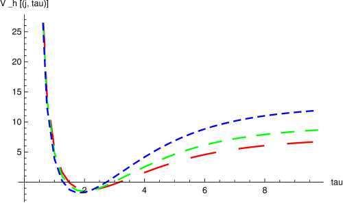
Figure 6: Plots versus $\tau$ of the effective radial potentials $V_{eff}(\tau)$ of graviton modes in the approximate metric firouz06 of the deformed conifold. The red-green-blue coloured curves drawn with dashes of decreasing sizes refer to the states of angular momenta $l=2,\ j=1,2,3$.

Table 5: Masses $\hat{E}^{(N_{\star},l,j)}_{m}$ of the ground state and first two radial excitations ($m=1,2,3$) for graviton modes in singlet and charged representations of angular momenta ($l=0,1,2,\ j=1,2,3$ in the approximate $S^{2}\times S^{3}$ geometry of the deformed conifold firouz06 and in ground state and first string oscillator excitation ($N_{\star}-1=0,\ 1)$.

$\ \hat{E}^{(N_{\star}-1,l,j)}_{m}\$	$j=1$	$j=2$	$j=3$
$m$	$1\ \ \ \ 2\ \ \ \ \ 3$	$1\ \ \ \ 2\ \ \ \ \ 3$	$1\ \ \ \ 2\ \ \ \ \ 3$
$\hat{E}^{(0,0,j)}_{m}$	${2.03\ \ \ 3.07\ \ \ 4.11}$	${3.62\ \ \ 4.72\ \ \ 5.78}$	${5.09\ \ \ 6.23\ \ \ 7.31}$
$\hat{E}^{(0,1,j)}_{m}$	${3.97\ \ \ 5.05\ \ \ 6.23}$	${4.52\ \ \ 6.25\ \ \ 7.48}$	${6.38\ \ \ 7.66\ \ \ 8.95}$
$\hat{E}^{(0,2,j)}_{m}$	${6.09\ \ \ 7.17\ \ \ 8.23}$	${6.89\ \ \ 7.96\ \ \ 9.07}$	${7.96\ \ \ 9.05\ \ \ 10.2}$
$\hat{E}^{(1,0,j)}_{m}$	${3.23\ \ \ 4.40\ \ \ 5.52}$	${4.28\ \ \ 5.44\ \ \ 6.55}$	${5.54\ \ \ 6.71\ \ \ 7.83}$
$\hat{E}^{(1,1,j)}_{m}$	${4.78\ \ \ 5.90\ \ \ 6.98}$	${5.66\ \ \ 6.77,7.85}$	${6.80\ \ \ 7.90\ \ \ 9.00}$
$\hat{E}^{(1,2,j)}_{m}$	${6.65\ \ \ 7.76\ \ \ 8.84}$	${7.35\ \ \ 8.45\ \ \ 9.53}$	${8.33\ \ \ 9.44\ \ \ 10.5}$

A.4 Undeformed conifold limit

We consider the approximate construct proposed in firouz06 using a large $\tau$ limit of the metric in the $S^{2}\times S^{3}$ geometry which leads to analytic solutions for the modes wave funnctioms analogous to those of the hard wall model chemtob16 . The modified effective potential is defined through the change of radial variable $\tau\to\rho$ by the ansatz

$$V_{eff}(\tau)=-{4\rho^{2}\over 9\nu^{2}}+V_{5}(\tau)+G_{1}(\tau),\ \ [\rho={\nu\lambda_{1}\over 2}e^{-{2\tau\over 3\nu}}={3^{1/2}\epsilon^{2/3}\lambda_{1}\over 2^{5/6}r},$$ (A.70)

$$G_{1}(\tau)\to G_{1}=4/9,\ \lambda_{1}=a\hat{E}_{m},\ V_{5}(\tau)\to Q^{2}=\hat{c}\hat{\mu}^{2}+\hat{d}(j^{2}-1)+\hat{f}l(l+1)+\hat{g}]$$ (A.71)

depending on the free adjustable parameters $a,\ \nu$ and $\hat{c},\ \hat{d},\ \hat{f},\ \hat{g}$ associated to the radial potential and the angular potential $V_{5}$. (Compare to the large $\tau$ limit for $T^{1,1}$ base manifold, $V_{5}(\tau)=-\tilde{g}_{\tau\tau}\tilde{\nabla}_{5}^{2}\simeq-\tilde{\nabla}{T^{1,1}}^{2}/9\to H_{0}^{\nu}/9$.) The modes wave functions are given by radial functions $R_{m}(\rho)=B_{m}(\rho)/G^{1/2}(\tau)$ times harmonic functions of $S^{3}$ and $S^{2}$, where the radial wave equation, $0=(\partial^{2}_{\tau}-V_{eff})B_{m}(\tau)$, can be solved in terms of Bessel functions,

$$0=(\rho\partial_{\rho}\rho\partial_{\rho}-{9\nu^{2}\over 4}\tilde{V}_{eff})B_{m}=(\rho^{2}B^{\prime\prime}_{m}+\rho B^{\prime}_{m}+(\rho^{2}-\tilde{\nu}^{2})B_{m}(\rho)),$$ (A.72)

$$\Longrightarrow\ B_{m}(\rho)={\rho^{2}\over N^{\prime}_{m}}(J_{\tilde{\nu}}(\rho)+b_{m}Y_{\tilde{\nu}}(\rho)),\ [\tilde{\nu}^{2}=\nu^{2}(1+{9Q^{2}\over 4})].$$ (A.73)

In the WKB quantization rule, analogous to Eq.(III.27), the phase integral for $V_{eff}=-{4\rho^{2}\over 9\nu^{2}}+Q^{2}+{4\over 9}$ over the interval between the origin and the potential turning point, $(\tau_{0}^{\prime}=0,\ \tau_{0})$, corresponding to the variable $z={\rho\over\tilde{\nu}}$ interval $(z_{0}=1,\ z^{\prime}_{0}={\nu\lambda_{1}/(2\tilde{\nu})})$, is given by

$$\pi(n-{1\over 2}+{\delta_{l,0}\over 4})=\int_{\tau^{\prime}_{0}}^{\tau_{0}}d\tau(-V_{eff}(\tau))^{1/2}=\tilde{\nu}\int_{z_{0}}^{z^{\prime}_{0}}dz{({z^{2}}-1)^{1/2}\over z}=\tilde{\nu}[(z^{{}^{\prime}2}_{0}-1)^{1/2}-\tan^{-1}((z^{{}^{\prime}2}_{0}-1)^{1/2})].$$ (A.74)

The fit to numerical values of masses for singlet modes in the warped deformed conifold case gave firouz06 , $\nu\approx 2.44,\ a\approx 2.48.$ The other constant parameters in $Q$ can then be determined by fitting the masses of string and charged modes in Table 5. Since our $Q$ is related to ${\cal Q}$ of firouz06 by $2(1+{9\over 4}Q^{2})^{1/2}/a={\cal Q}$, which for modes of large charges becomes, $Q\simeq a{\cal Q}/3$, our (hatted) parameters for $Q$ can be evaluated from the (unhatted) ones of firouz06 using $[\hat{c},\ \hat{d},\ \hat{f},\ \hat{g}]=(a/3)[c,\ d,\ f,\ g]\approx 0.83\times[3.4,\ 1.4,\ 3.4,\ 0.65].$

References

- (1) M.R. Douglas and S. Kachru, Rev. Mod. Phys. 79, 733 (2007) [arXiv:hep-th/0610102]
- (2) M. Grana, Phys. Rep. 423, 91 (2006) [arXiv:hep-th/0509003]
- (3) O. Aharony, S.S. Gubser, J. Maldacena, H. Ooguri, and Y. Oz, Phys. Rep. 323, 183 (2000) [arXiv:hep-th/9905111]
- (4) L. Randall and R. Sundrum, Phys. Rev. Lett. 83, 3370 (1999) [arXiv:hep-ph/9905221]
- (5) L. Randall and R. Sundrum, Phys. Rev. Lett. 83, 4690 (1999) [arXiv:hep-th/9906064]
- (6) K. Becker and M. Becker, [arXiv:hep-th/9605053]
- (7) B.S. Acharya, J.M. Figueroa-O’farrill, C.M. Hull, and B. Spence, [arXiv:hep-th/9808014]
- (8) H. Verlinde, [arXiv:hep-th/9906182]; E. Verlinde and H. Verlinde , [arXiv:hep-th/9912018]; C.S. Chan, P.L. Paul, and H. Verlinde, [arXiv:hep-th/0003236]; H. Verlinde, [arXiv:hep-th/0004103]
- (9) K. DasGupta, G. Rajesh, and S. Sethi, [arXiv:hep-th/9908088]
- (10) K. Becker and M. Becker, [arXiv:hep-th/0010282]
- (11) B. Greene, K. Schalm, and G. Shiu, [arXiv:hep-th/0004103]
- (12) K. Becker and M. Becker, [arXiv:hep-th/0107044]
- (13) S.B. Giddings, S. Kachru, and J. Polchinski, Phys. Rev. D66, 106006 (2002) [arXiv:hep-th/0105097]
- (14) S.P. de Alvis, [arXiv:hep-th/0307084]
- (15) S.B. Giddings and A. Maharana, [arXiv:hep-th/0507158]
- (16) H. Firouzjahi and S.-H.H. Tye, JHEP C01, 136 (2006) [arXiv:hep-th/0512076]
- (17) M. R. Douglas, J. Shelton, and G. Torroba, [arXiv:0704.4001]
- (18) M.R. Douglas and G. Torroba, [arXiv:0805.3700]
- (19) G. Shiu, G. Torroba, B. Underwood, and M.R. Douglas, JHEP C0806, 024 (2008) [arXiv:0803.3068]
- (20) A. Frey, G. Torroba, B. Underwood, and M.R. Douglas, [arXiv:0810.5768]
- (21) M.R. Douglas, [arXiv:0911.3378]
- (22) A.R. Frey and J. Roberts, [arXiv:1308.0323]
- (23) L. Kofman and P. Yi, [arXiv:hep-th/0507257]
- (24) X. Chen and S.H.H. Tye, J. Cosm. Astr. Phys. (JCAP) 06, 011 (2006) [arXiv:hep-th/0602136]
- (25) A. Berndsen, J.M. Cline, and H. Stoica, Phys. Rev. D77, 123522 (2008) [arXiv:0710.1299]
- (26) J.F. Dufaux, L. Kofman, and M. Peloso, [arXiv:0802.2958]
- (27) A.R. Frey, R.J. Danos, and J.M. Cline, [arXiv:0908.1387]
- (28) M. Chemtob, [arXiv:1909.07668]
- (29) P. Candelas and X.C. de la Ossa, Nucl. Phys. B342, 246 (1990)
- (30) I. Klebanov and M.J. Strassler, JHEP C08, 052 (2000), [arXiv:hep-th/0007191]
- (31) H. Kim, L. Romans, and P. van Nieuwenhuizen, Phys. Rev. D32, 389 (1985)
- (32) A. Ceresole, G. Dall’Agata, R. D’Auria, and S. Ferrara, Phys. Rev. D542, 273 (1999) [arXiv:hep-th/9905226]
- (33) A. Ceresole, G. Dall’Agata, R. D’Auria, JHEP C11, 009 (1999) [arXiv:hep-th/9907216]
- (34) I.R. Klebanov and E. Witten, Nucl. Phys. B536, 199 (1998) [arXiv:hep-th/9807080]
- (35) S. Kachru, R. Kallosh, A.D. Linde, and S.P. Trivedi, [arXiv:hep-th/0301240]
- (36) S. Kachru, R. Kallosh, A.D. Linde, J. Maldacena, L. McAllister, and S.P. Trivedi, [arXiv:hep-th/0308055]
- (37) D. Baumann, A. Dymarsky, I.R. Klebanov, J. Maldacena, L. McAllister, and A. Murugan, [arXiv:hep-th/0607050]
- (38) D. Baumann, A. Dymarsky, S. Kachru, I.R. Klebanov and L. McAllister, [arXiv:0706.0360]
- (39) N. Barnaby, C.P. Burgess, and J.M. Cline, [arXiv:hep-th/0412040]
- (40) A.R. Frey, A. Mazumdar, and R. Myers, [arXiv:hep-th/0508139]
- (41) D. Chialva, G. Shiu, and B. Underwood, JHEP C01, 014 (2006) [arXiv:hep-th/0508229]
- (42) D. Chialva, P.S. Bhupal Dev, and A. Mazumdar, [arXiv:1211.0250]
- (43) X. Chen, [arXiv:hep-th/0902.0008]
- (44) S. Gandhi, L. McAllister, and S. Sjors, [arXiv:1106.0002]
- (45) S.S. Pufu, I.R. Klebanov, T. Klose, and J. Lin, [arXiv:1009.2763]
- (46) R. Minasian and D. Tsimpis, [arXiv:hep-th/9911042]
- (47) I.R. Klebanov and A.A. Tseytlin, Nucl. Phys. B578, 2000 (123) [arXiv:hep-th/0002159]
- (48) C.P. Herzog, I.R. Klebanov, and P. Ouyang, [arXiv:hep-th/0108101]
- (49) M.B. Douglas, J. Shelton, and G. Torroba, [arXiv:hep-th/0704.4001]
- (50) C.M. Brown and O. DeWolfe, [arXiv:hep-th/0901.4401]
- (51) K. Choi, A. Falkowski, H.P. Nilles, and M. Olechowski, [arXiv:hep-th/0503216]
- (52) V. Balasubramanian, P. Berglund, J.P. Conlon, and F. Quevedo, [arXiv:hep-th/0502058]
- (53) R. Blumenhagen, S. Moster, and E. Plauschin, [arXiv:0711.3389]
- (54) R. Blumenhagen, J.P. Conlon, S. Krippendorf, S. Moster, and F. Quevedo, [arXiv:0906.3297]
- (55) C. Krishnan and S. Kuperstein, [arXiv:0802.3674]
- (56) D.A. Levine, Trans. Amer. Math. Soc. 144 (1969) 493
- (57) S.S. Gelbart, Trans. Amer. Math. Soc. 192 (1974) 29
- (58) M. Berg, M. Haack, and W. Mück, [arXiv:hep-th/0507285]; [arXiv:hep-th/0612224]
- (59) R. de Mello Koch, A. Jevicki, M. Mihailescu, and J.P. Nunes, Phys. Rev. D58, 105009 (1998) [arXiv:hep-th/9806125]
- (60) M. Zyskin, [arXiv:hep-th/9806128]
- (61) C. Csaki, H. Oguri, Y. Oz, and J. Terning, [arXiv:hep-th/9806021]
- (62) J.A. Minahan, [arXiv:hep-th/9811156]
- (63) J. G. Russo and K. Sfetsos, [arXiv:hep-th/9901056]
- (64) L.D. Landau and E.M. Lifshytz, Quantum Mechanics (1958, Pergamon Press)
- (65) E. Merzbacher, Quantum Mechanics, (1970, John Wiley and Sons)
- (66) M.V. Berry and K.E. Mount, Rep. Prog. Phys. 35, 315 (1972)
- (67) C. M. Bender and S. A. Orszag, ‘Advanced Mathematical Methods for Scientists and Engineers: Asymptotic Methods and Perturbation Theory’ (McGraw Hill, New York, 1978), (Springer-Verlag, 1999)
- (68) M. Krasnitz, [arXiv:hep-th/0011179]; [arXiv:hep-th/0209163]
- (69) E. Caceres and R. Hernandez, [arXiv:hep-th/0011204]
- (70) M.K. Benna, A. Dymarsky, I.R. Klebanov, and A. Solovyov, [arXiv:0712.4404]
- (71) A. Frey and A. Maharana, [arXiv:hep-th/0603232]
- (72) H. Davoudiasl, J.L. Hewett, and T.G. Rizzo, [arXiv:hep-ph/0211377]
- (73) B. Grzadkowski and J.F. Gunion, [arXiv:hep-ph/0610105]
- (74) K.R. Dienes, E. Dudas, and T. Ghergetta, [arXiv:hep-th/9908530]
- (75) C.P. Burgess, P.G. Camara, S.P. de Alwis, S.B. Giddings, A. Maharana, F. Quevedo, and K. Suruliz, [arXiv:hep-th/0610255]
- (76) S.P. de Alvis, [arXiv:hep-th/1202.1546]
- (77) M. Marino, R. Minasian, G. Moore, and A. Strominger, [arXiv:hep-th/9911206]
- (78) J.P. Gauntlett, [arXiv:hep-th/0305074]
- (79) L. Martucci and J. Smyth, [arXiv:hep-th/0507099]; L. Martucci, [arXiv:hep-th/0602129]
- (80) D. Lüst, F. Marchesano, L. Martucci and D. Tsimpis, JHEP C11, 021 (2008) [arXiv:0807.4540]
- (81) F. Marchesano, P. McGuirk, and G. Shiu, [arXiv:0812.2247];
- (82) F. Marchesano, P. McGuirk, and G. Shiu, [arXiv:1012.2759]
- (83) G. Shiu, B. Underwood, D.G.E. Walker, and K. Zurek, [arXiv:0705.4097]
- (84) P. McGuirk, G. Shiu, and K.M. Zurek, JHEP C03, 012 (2008) [arXiv:0712.2264]
- (85) N. Lambert, H. Liu and J. Maldacena, [arXiv:hep-th/0303139]
- (86) C.M. Bender and S. Sarkar, [arXiv:1203.1822]
- (87) S. Weinberg, ‘Cosmology’ (Oxford Press, 2008)
- (88) M. Cvetic, G.W. Gibbons, H. Lu, and C.N. Pope, Comm. Math. Phys. 232, 457 (2003) [arXiv:hep-th/0012011]
- (89) F. Benini, A. Dymarsky, S. Franco, S. Kachru, D. Simic, and H. Verlinde, JHEP C12, 031 (2009) [arXiv:0903.0619]
- (90) E.G. Gimon, L.A. Pando Zayas, J. Sonnenschein, and M.J. Strassler, [arXiv:hep-th/0212061]
- (91) P. McGuirk, G. Shiu, and F. Ye, [arXiv:1206.0754]
- (92) S. Kuperstein, [arXiv:hep-th/0411097]
- (93) S. Kuperstein and J. Sonnenschein, [arXiv:hep-th/0807.2897]
- (94) G. Papadopoulos and A.A. Tseytlin, [arXiv:hep-th/0012034]
- (95) D. Martelli and J. Sparks, Comm. Math. Phys. 262, 51 (2006) [arXiv:hep-th/0411238]
- (96) S. Benvenuti, S. Franco, A. Hanany, D. Martelli, and J. Sparks, JHEP C06, 064 (2005) [arXiv:hep-th/0411264]
- (97) C.P. Herzog, Q.J. Ejaz, and I.R. Klebanov, JHEP C02, 009 (2005) [arXiv:hep-th/0412193]
- (98) S. Benvenuti, S. Franco, A. Hanany, D. Martelli, and J. Sparks, [arXiv:hep-th/0411264]
- (99) F. Canoura, J.D. Edelstein, L.A. Pando Zayas, A.V. Ramallo, and D. Vaman, [arXiv:hep-th/0512087]
- (100) U.H. Gerlach and U.K. Sengupta, Phys. Rev. D18, 1773 (1978)