Local dominance unveils clusters in networks

Abstract

Clusters or communities can provide a coarse-grained description of complex systems at multiple scales, but their detection remains challenging in practice. Community detection methods often define communities as dense subgraphs, or subgraphs with few connections in-between, via concepts such as the cut, conductance, or modularity. Here we consider another perspective built on the notion of local dominance, where low-degree nodes are assigned to the basin of influence of high-degree nodes, and design an efficient algorithm based on local information. Local dominance gives rises to community centers, and uncovers local hierarchies in the network. Community centers have a larger degree than their neighbors and are sufficiently distant from other centers. The strength of our framework is demonstrated on synthesized and empirical networks with ground-truth community labels. The notion of local dominance and the associated asymmetric relations between nodes are not restricted to community detection, and can be utilised in clustering problems, as we illustrate on networks derived from vector data.

INTRODUCTION

Many real-world datasets can be viewed as a collection of objects embedded into a global metric space, thereby providing a vector representation [1]. Alternatively, networks have become another fundamental way to model complex systems with a focus on direct pairwise interactions between constituents [2, 3, 4]. In the case of social systems, for instance, these complementary representations may correspond to a set of socio-demographic variables for each individual, e.g., in a Blau space [5], or to a social network of interactions between individuals, e.g., via a mobile communication network [6] or spatio-temporal co-occurrence interactions [7]. In each representation, real-world systems tend to exhibit groups: regions of high density in the spatial representation, known as clusters, or high density subgraphs in the network, known as communities. Such cluster or community structure provides a coarse-grained representation of the underlying complex system[8, 9, 10, 11], often associated to different functions and impacting its collective behaviours [12, 13, 14], and their unsupervised detection is thus essential in different areas of data science [1, 10].

In the vector representation, the introduction of a dissimilarity function and ideally of a distance in a metric space, provides a natural way to identify the centre of a cluster, e.g., the medoid in a general metric space [15, 16], and a hierarchy would form within a cluster between central and other more peripheral nodes, implying an asymmetric relationships between them. On the other hand, in the case of asymmetric pairwise interactions, which can be associated to an implicit hierarchy [17] and have long been recognized [18, 19, 20, 21, 22] in various network systems, community detection methods for networks place much less emphasis on the concept of community center and hierarchy within communities. We can always use network centrality measures on the subgraphs identified as communities to identify core and peripheral nodes a posteriori, but these roles are not central to community detection [23, 24], in stark contrast to clustering methods based on embedding the data in a metric space.

In this paper, we propose a community detection algorithm in networks, Local Search (LS), that explicitly uses the notion of local dominance and identifies community centres based on local information. In our method, every node is given at most one parent node deemed to be higher up in a partial ranking. Nodes that have a dominant position in their immediate neighborhood [18] or even beyond are identified as local leaders [18]. This defines a rooted tree that spans the network and gives rise to community centers that are local leaders [18] with both a larger degree than the nodes in their basin of attraction and a relatively long distance to other local leaders higher up in the ranking. Our approach possesses several interesting properties. Firstly, it provides a new perspective on community detection and delivers community centres and a hierarchy within the community and even a hierarchy among communities as an explicit part of our algorithm, and so mimics advantageous features of the methods based on embedding data in a metric space. Secondly, the identification of communities through local dominance is highly efficient, as it uses purely local topological information and breadth-first search, and runs in linear time. The method does not require the heuristic optimization of an objective function that relies on a global null model[9, 25, 26, 27, 28, 29] or computationally costly spreading dynamics[30, 31, 32]. Also, our method does not rely on a similarity measure for which there is an wide choice, with an associated uncertainty and variability in results, such as is found in hierarchical clustering based methods [8, 33, 34, 14]. Finally, LS is not as susceptible to noise as most methods[35, 10], and is less therefore susceptible to finding spurious communities in random graph model realisations[36].

We demonstrate the strength of LS on several classical but challenging synthetic benchmarks and on standard empirical networks with known ground-truth community labels. Our numerical evaluation also includes network representations derived from vector data. As the LS method naturally provides community centres and local hierarchies, it creates an explicit analogy with the notion of cluster centres and distances within clusters that are found in vector clustering methods. Moreover, we also show that applying LS on discretised version of data cloud points outperforms classical unsupervised vector data clustering methods on benchmarks [16].

MATERIALS AND METHODS

The Local Search (LS) algorithm

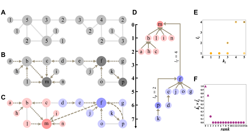
Figure 1: Schematic illustration of the Local Search (LS) algorithm. (A) An example network where digits on nodes and size of nodes indicate the degree. (B) The identification of local leaders based on local dominance by creating a forest of DAGs as indicated by short dashed directed edges. For each node $u$, it points to any adjacent neighbor $v$ with $k_{v}\geq k_{u}$ and $k_{v}=\max\{k_{z}|z\in\mathbf{V}(u)\}$, where $\mathbf{V}(u)$ is the set of neighboring nodes. In this example, nodes are traversed by their lexicographical order, when node b is traversed, it points to m as $k_{m}=\max\{k_{z}|z\in\mathbf{V}(b)\}\geq k_{b}$; later, when m is traversed, it has no out-going link, and so m is identified as a local leader: it does not point to any of its followers and its remaining neighbors all have smaller degrees. When there are more than one neighbor with the same largest degree, more than one directed edge is temporarily added, e.g., node c points to both b and m as $k_{b}=k_{m}=\max\{k_{z}|z\in\mathbf{V}(c)\}\geq k_{c}$; nodes d and l also have more than one outgoing link. The local leaders, which are potential community centers, are $f$, $m$, and $p$ (indicated by dark grey color). (C) Each node randomly retains just one out-going edge shown as a short dashed directed edge (e.g., c can point to b or m with an equal probability, similarly for l and d). Then, for each local leader $u$, a local-BFS is performed to find its nearest local leader with $k_{v}\geq k_{u}$, and the shortest path length on network $d_{uv},\forall v$ is designated by $l_{u}$. Here, $p\rightarrow f$ with $l_{p}=2$, and $f\rightarrow m$ with $l_{f}=4$. In (C), short-dash arrows and long-dash arrows correspond to pure followers (whose $l_{u}=1$) and local leaders (whose $l_{u}\geq 2$), respectively. Each node has at most one out-going link $(u\rightarrow v)$, which can go beyond direct connections. The local leader(s) with the maximal degree has no out-going link (here node m). (D) The corresponding tree structure formed by local dominance. The scale on the left is a visual aid for calculating $l_{i}$ between connected nodes in the DAG. (E) The scatter plot of $k_{i}$ and $l_{i}$ for all nodes. Community centers are of both a larger degree $k_{i}$ and a longer $l_{i}$. (F) The decision graph for quantitatively determining community centers (indicated by triangles) based on the product of rescaled degree $\tilde{k}_{i}$ and rescaled distance $\tilde{l}_{i}$ (see more details in Supplementary Text A.2). Community centers can be detected by a visual inspection for obvious gaps or sophisticated automatic detection methods. Here, two centers, nodes m and f, are identified. The color of nodes in (C) and (D) represents the community partition, and community centers are highlighted by a darker hue of the same color.

Cluster analysis and community detection share many conceptual similarities, but often have a contrasting focus. Cluster analysis puts emphasis on the centre of a cluster [15, 16], while community boundaries often play a more predominant role in community detection [37]. Community centres can be inferred from some community detection algorithm outputs, for example, the nodes associated to the largest absolute weights of the leading eigenvector of the modularity matrix, or exhibiting a higher density of connections inside the communities, are deemed to be community centers, core members or provincial hubs [23, 38]. But centres are only a by-product of the algorithm, rather than at their core of methodologies.

The approach that we propose here is explicitly focusing on community centres to identify clusters, which is motivated by the existence of underlying asymmetries between nodes [19, 20, 21], the concept of local leaders [18] in networks and borrows ideas from density and distance based clustering algorithms on vector data [16]. We hypothesise that a community center is a local leader that is comparatively of a larger degree than its neighbors, thus “dominating” them, and is of a relatively long shortest-path distance to other local leaders.

Our algorithm consists of four steps that we now detail. We start with an undirected network with $N$ nodes and $E$ edges, for example see Fig. 1A. For better clarity, nodes are also labeled and traversed in lexicographical order (see Fig. 1B).

1. First, we calculate the degree $k_{u}$ of each node $u$ (see digits in Fig. 1A), which is an operation of linear time complexity O$(E)$.

2. Second, we traverse each node $u$ and point $u$ to any adjacent node $v$ with $k_{v}\geq k_{u}$ and $k_{v}=\max\{k_{z}|z\in\mathbf{V}(u)\}$ (i.e., $v$ has the largest degree in the neighborhood of $u$). For example, in Fig. 1B node g will point to f instead of p as $k_{f}>k_{p}>k_{g}$; and c points to both b and m as $k_{b}=k_{m}=\max\{k_{z}|z\in\mathbf{V}(c)\}>k_{c}$. Note that a node cannot point to its follower, and since nodes are traversed in lexicographical order, when node b is traversed, it will point to m as $k_{m}=\max\{k_{z}|z\in\mathbf{V}(b)\}\geq k_{b}$. When m is traversed, it will not point to any of its followers (e.g., b). This process naturally avoids the creation of loops and ensure we only obtain directed acyclic graphs (DAGs), see Fig. S1 and proof in Supplementary Text A.1.1 for more details. If such a $v$ does not exist, $u$ will not have any outgoing edge and will be identified as a local leader (see dark grey nodes f, p, and m in Fig. 1B). We denote the set of local leaders as $\mathbf{C}$.

   After traversing all nodes, for nodes with multiple out-going links, we randomly retain one (see only short dash arrows in Fig. 1C for a possible mapping). Mathematically, we have obtained a forest of trees, where the root of each tree is a local leader, and is also a potential community center. For most nodes, except local leaders, this process identifies a local hierarchy (indicated by dash arrows), with an asymmetric leader-follower relation (see short-dash arrows in Fig. 1B). This step is completed in O$(E)$.

3. Third, to identify the upper level for local leaders along the hierarchy, we use a local breadth-first search (BFS) starting from each local leader $u$ and stop the search when encountering the first local leader $v$ with $k_{v}\geq k_{u}$ and assign the shortest path length on the original network $d_{uv}$ to $l_{u}$, which is the length of the out-going link of node u. Note that $l_{u}\geq 2$ for all local leaders, and all pure followers have $l_{u}=1$. For example, node p is a local leader, in the second iteration of the BFS, it encounters another local leader f with $k_{f}>k_{p}$. We stop the local-BFS and point p to f, and $l_{p}=d_{pf}=2$. Similarly, $f\rightarrow m$ and $d_{mf}=4$. The out-going link of local leaders goes beyond the direct connections in the original network (see long-dash arrows in Fig. 1C).

   When there are several local leaders that have a no smaller degree than the local leader $u$ in the $l_{u}^{th}$ iteration, the largest one is chosen; if multiple nodes have the same largest degree, one is picked at random uniformly. For local leader(s) with the maximal degree in the whole network, denoted as $\mathbf{M}$, a subset of $\mathbf{C}$, there is no need to perform the BFS, and we directly assign $l_{x\in\mathbf{M}}=\max_{u\in\mathbf{C}\setminus\mathbf{M}}({l_{u}})$.

   Community centers can be easily identified as local leaders with both a large $k_{u}$ and a long $l_{u}$ (see Fig. 1E), and naturally emerges from the rooted tree revealed by local dominance (see all dash arrows in Fig. 1C and the explicit tree structure in Fig. 1D). We use the product of rescaled degree $\tilde{k}_{i}$ and rescaled distance $\tilde{l}_{i}$ to quantitatively measure the “centerness” of each node (see more details and discussions in Supplementary Text A.2). Community centers can be determined via visual inspection for obvious gaps or by automated detection methods (see Fig. 1F). For example, the community centers identified by the LS method in Fig. 1 are nodes f and m. In the Zachary Karate Club network, the identified community centers correspond to the president and the instructor, which is consistent with reality [39] (see Fig. S6).

   Theoretically, this third step takes O$\left((|\mathbf{C}|-|\mathbf{M}|)\langle k\rangle^{\langle l\rangle_{\mathbf{C\setminus M}}}\right)$=O$\left((|\mathbf{C}|-|\mathbf{M}|)E\right)$, where $\langle k\rangle$ is the average degree of the network, $\langle l\rangle_{\mathbf{C\setminus M}}=\sum_{u\in\mathbf{C\setminus M}}l_{u}/(|\mathbf{C}|-|\mathbf{M}|)$, and the size of the set of potential centers $|\mathbf{C}|$ is usually much smaller than $N$ (see Table S1). In practice, $\langle k\rangle^{\langle l\rangle_{\mathbf{C\setminus M}}}$ is bounded to be smaller than $E$ as it mimics a local-BFS process. As indicated by numerical results, even $(|\mathbf{C}|-|\mathbf{M}|)\langle k\rangle^{\langle l\rangle_{\mathbf{C\setminus M}}}$ is usually smaller than $E$ (see Table S1). In addition, the local-BFS process can be simultaneously implemented for all local leaders in parallel to further speed up the algorithm in practice.

4. Finally, for all identified community centers, we remove their out-going links, if any. Community labels are then assigned along the reverse direction of directionality $u\leftarrow v$ from community centers. This step takes again a linear time O($N$).

Taken together, the time complexity of our LS algorithm is linear: O$\left(E+(|\mathbf{C}|-|\mathbf{M}|)\langle k\rangle^{\langle l\rangle_{\mathbf{C\setminus M}}}+N\right)=\Theta(E)$, which is among the fastest community detection algorithms. Our framework provides a new perspective on community detection methods. It only relies on the notion of local dominance, which is identified solely from local information from the topology. It does not need to iteratively optimize an objective function [9, 26, 27, 28, 29] based on a global randomized null model [23, 9, 27] or resorting to iterative spreading dynamics [30, 31] as other state-of-the-art algorithms. It is important to emphasise that the communities that are uncovered by LS are not necessarily associated to a high density of links, as in modularity optimisation, or specific patterns of connectivity inside versus across groups, as in methods based on stochastic block models [40, 41, 42], but are instead obtained as a group of nodes that are dominated by the same leader.

RESULTS

In this section, we first test our method on a series of synthetic networks to benchmark its performance and its multiscale community detection capacity, before analysing real-world networks. Finally, we show how it outperforms current state-of-the-art unsupervised both clustering and community detection methods when applied to discretised vector data clouds. The implementation of our algorithm was done in Python and we use the NetworkX package implementation of the Louvain algorithm, our main point of comparison in this section, to obtain fair comparison of running time.

Synthetic networks

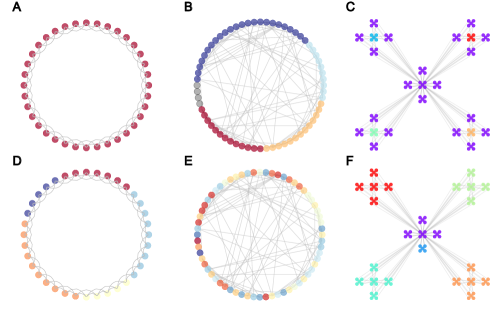
Figure 2: Community partitions by the LS and Louvain algorithms on synthesized networks with different strength of heterogeneity. The heterogeneity increases from left to right. The color of nodes denotes the community membership. In a strict homogeneous regular network ($N=36,\langle k\rangle=4$), all nodes are identical, (A) only one community is detected by the LS algorithm (see Fig. S1 for more details); (D) by contrast, the Louvain algorithm detects five communities by optimizing modularity. In an Erdős-Rényi random network ($N=64,\langle k\rangle=4$), there may exist some communities due to randomness [36], (B) the LS algorithm detects fewer communities compared to (E) the Louvain algorithm (see Fig. S2). In a Ravasz-Barabási network [43] which displays stronger heterogeneity, (C) the LS algorithm groups all first-level nodes and all sixteen second-level peripheral clusters into one community, and four small communities emerge (see Fig. S4 for more details); (F) the Louvain algorithm partitions each second-level branching as a separate community and misclassifies a first-level peripheral cluster into its own community, a result of traversal order and modularity optimization process in the Louvain algorithm.

Here, we use well-known benchmark networks to illustrate how the LS method functions and in which situations it performs well. We contrast the results obtained by the LS method to those obtained by the well-known Louvain method [9] that optimises modularity roughly in linear time in practice. We first look at a circular regular network, where all nodes are equivalent and thus no community structure should be discovered. LS correctly identifies a single community (Fig. 2A), by contrast, modularity forces community structure to exist and finds five communities (Fig. 2D). Let us look in detail at the reason why LS finds a single community. First, each node will point to all its adjacent neighbors as they all have the same degree, and since node are sequentially traversed and they will not point to their followers, loops cannot be formed, see Fig. S1C and Supplementary Text A.1.1 for a proof. After all nodes have been considered, each node will only keep one outgoing link with an equal probability, and eventually a tree structure will be formed. Because of the homogeneity of the graph, the tree only allows the identification a single community centre and therefore of a single community. Because all nodes are equivalent, the labeling and thus order in which they are visited, is irrelevant. We note that in the case of a clique, an extreme case of regular network, the mapping of local hierarchy can yield a range of structure from a chain to a star structure, see Fig. S1B for more details. In all cases, only one centre is identified. By contrast, the Louvain method would partition a homogeneous regular network into several communities by optimizing modularity (see Fig. 2D).

Our second application focuses on Erdős-Rényi (ER) random graphs. While in the limit of an infinite random graph no community structure exists, in finite-size ER graphs, fluctuations may create spurious community structures [36, 11]. In this example, the LS method detects fewer communities than the Louvain algorithm, see Fig. 2B and E. In ER random networks, the degree distribution is relatively peaked around its average, but the system nonetheless exhibits fluctuations in the degrees. Large degree nodes are more likely to connect to each other, as the connection probability between them, $k_{i}k_{j}/2E$, are among the highest ones. When two large nodes are connected, there will be a directed out-going link pointing from one node to the other, making one of them a follower. Thus the LS method detects fewer communities. On the other hand, when we fix the size of the network and increase the connection probability $p$, the number of communities detected by the Louvain algorithm also decreases but it consistently finds more communities than the LS method (see Fig. S2). In addition, we are able to detect isolated nodes as noise (see grey nodes in Fig. 2B), as these nodes are of a small degree but infinite $l_{i}$.

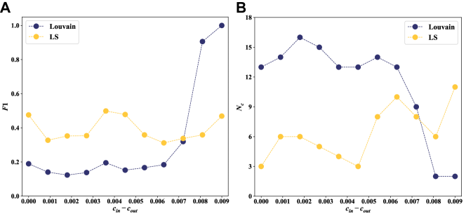
Fig. S3: The comparison between the Louvain algorithm and our LS method on synthesized networks by stochastic block model (SBM). (A) The $F_{1}$-score and (B) the number of communities $N_{c}$ detected by the LS and Louvain algorithms. We generate networks with two communities by SBM, each of which has 1,000 nodes. $c_{in}=0.009$ is the density of edges between nodes the same group, and $c_{out}$ is the density of edges between nodes from different groups. We gradually increase $c_{out}$ until it equals $c_{in}$.

We also consider an extension of the ER random graph model, the stochastic block models shown in Fig. S3 and discussed in Supplementary Text A.1.2. For random networks generated by stochastic block model [40, 41, 42] with two blocks, when the inter-connection probability is zero, $c_{out}=0$, the Louvain algorithm detects two communities that align with ground truth, but also reflects the resolution limit [44]. By contrast, the LS algorithm still detects as many community centers as when looking at each individual random network. This result can be understood by the local nature of the algorithm, where the structure of one disconnected cluster does not affect the communities found in the other and thus LS algorithm does not suffer from resolution limit. When we fix the intra-connection probability $c_{in}$ and gradually increase $c_{out}$, the boundary of the two communities becomes blurred. In this case the $F_{1}$-score of the LS algorithm is relatively stable, though not too high (see Fig. S3), while the performance of Louvain algorithm decreases quickly (see Fig. S3A) and the number of communities found by the Louvain algorithm increases (see Fig. S3B).

Finally, we consider a hierarchical benchmark, the Ravasz-Barabási network model [43] with two layers, which naturally provides a model with a hierarchy between the center and peripheral nodes. The clustering proposed by LS method groups explicitly reflects the hierarchical nature of the model by grouping first-level nodes and all sixteen second-level peripheral clusters into one community centred at the original seed node, as it dominates their neighborhood. Four small communities emerge due to the existence of four centers, which hav a degree larger than their neighbours and a longer path length to the original seed node, i.e., $l_{i}>1$, see Fig. S4C for the decision graph. The Louvain algorithm offers an alternative partitioning that ignores the hierarchical nature of the model and finds five communities of roughly equal size and one small community (see Fig. 2F). This example is interesting in that the clustering provided by Louvain here provides a reasonable, yet alternative, answer that ignores one aspect of the data. This reminds us that different clustering methods rely on different underlying mechanisms and, as often occurs when using unsupervised methods, the outputs are rarely strictly right or wrong. The outputs should be understood not only in terms of the data, but of the methods as well. Still, it is worth noting that the Louvain algorithm misclassifies a first-level peripheral cluster into another community (see the blue cluster in Fig. 2F), due to the traversal order used by the algorithm and modularity optimization process (see Supplementary Text A.1.3 for more details). When we further modify the network generated by the Ravasz-Barabási model by adding a third-level branching to one of the second-level central cluster, and add noise in the connectivity to other second-level central clusters, the LS method still detects meaningful hierarchical structure, see Fig. S4B and D.

Detection of multiscale community structure

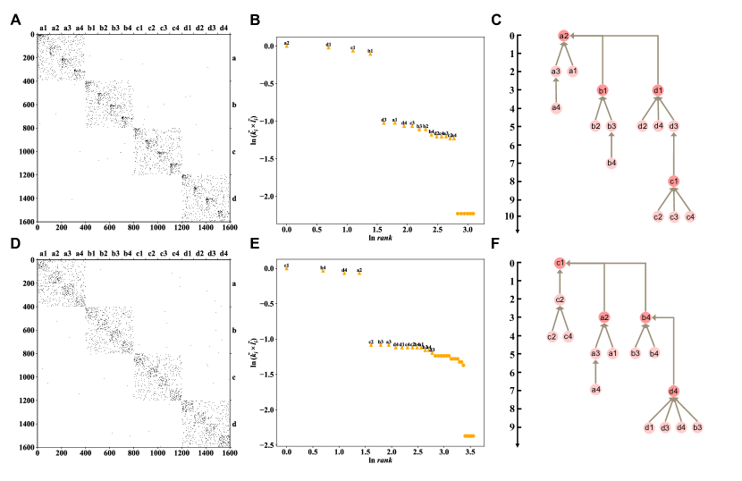
Figure 3: Detection of multiscale community structure with different heterogeneity. Both networks (A and D) comprise four top-level communities (labeled as a, b, c, and d) with 400 nodes each and an inter-connection probability $p_{1}=0.0002$, each of which further comprises four second-level communities with 100 nodes and $p_{2}=0.035$ (e.g., community c comprises c1, c2, c3, and c4). The second-level communities are generated by (A) the Barabási-Albert model [45] with $m=7$, (D) the Erdős-Rényi random network with a connection probability $p=0.14$ that both yield the same average degree $\langle k\rangle=14$. (B) and (E) show the decision graph for the LS method. For better clarity, only top sixteen nodes are labeled. (C) and (F) display the tree structure formed by the local dominance between identified centers of each community. For better clarity, community centers are named by the community label instead of the real index of the node, and we only show the tree structure of these centers. The height difference indicates the $l_{i}$ of the lower node. For the multiscale network in A, the LS method detects four top-level communities with $F_{1}=0.99$ and 16 second-level communities with $F_{1}=0.56$. For the network in D, the LS method detects four top-level communities with $F_{1}=0.89$ and 29 second-level communities with $F_{1}=0.29$. In both cases, the Louvain algorithm only obtain four top-level communities with $F_{1}$ equals $1$ and $0.40$ for evaluations at the first- and second-level, respectively. Results shown here correspond to just one realization, in multiple realizations, as every first- and second-level communities are equivalent, the label sequence in B and E and the tree structure in C and F may vary but have a consistent structure.

As partially reflected in the decision graph of the LS algorithm for the Ravasz-Barabási network (Fig. S4C and D), the reliance on local dominance of our method to identify local leaders naturally lends itself to detect multiscale community structure [34, 14, 46]. To illustrate this point, we generate a multiscale network made of two levels: four top-level communities with 400 nodes each and inter-connection probability $p_{1}=0.0002$, each top level community contains four second-level communities with 100 nodes each and $p_{2}=0.035$ [34, 14]. Each second-level community is generated by the standard Barabási-Albert model [45] with $m=7$ that yields $\langle k\rangle=14$ (see Fig. 3A). The LS method correctly identifies two levels of community structure with a notable gap between first four top-level centers, which have similar $\tilde{k}_{i}\times\tilde{l}_{i}$, and other potential centers, as shown in Fig. 3B. Then taking the twelve subsequent centers, these sixteen centers together correspond to the sixteen second-level communities, and their affiliation within each top-level communities are correct (see the tree structure for local leaders in Fig. 3C). As all sixteen second-level communities are statistically equivalent, the directionality of community centers (Fig. 3C) is determined by fluctuations in the network generating mechanism. The partition obtained by the LS method has an $F_{1}$-score of 0.99 at the top level and of $F_{1}=0.56$ at the second level. Misclassifications at the second level mainly come from a relatively large inter-connection probability $p_{2}$, which blurs the boundary between communities. In comparison, the Louvain algorithm only detects four large communities at the top-level but no further smaller communities due to the resolution limit [44]. The $F_{1}$-score of partitions by the Louvain algorithm equals $1$ and $0.40$ for the top-level and second-level evaluations, respectively. This demonstrate the strength of the LS method on detecting smaller scale community structure.

One reason that LS works on detecting multiscale structure resides in the fact that the average path length between nodes is governed by the connection probability [47]. The distance between nodes from different second-level communities within the same top-level community is on average shorter than the distance between nodes from different top-level communities, and thus the hierarchical structure is uncovered by the LS method. Another reason is the intrinsic heterogeneity in each second-level community.

By contrast, when keeping the average degree and inter-connection probability ($p_{1}$ and $p_{2}$) the same, and replacing the second-level communities by ER random networks with $p=0.14$, which also yields $\langle k\rangle=14$ (see Fig. 3D), the whole network becomes more homogeneous (see Fig. S5). In this case, the LS method can still detect four top-level communities (see Fig. 3E) but mis-identify some second-level communities (e.g., communities c2 and d1 are missing in this example, see Fig. 3F) and detect more smaller communities (29 second-level communities are detected instead of 16). The mis-identification of some second-level communities is due to the largest degree node $u$ in those ground-truth communities being directly connected to a node $v$ in other communities with $k_{v}\geq k_{u}$, and thus $u$ is considered as followers. This is more common in such a random setting, as there are more nodes with a relatively large degree beyond the reference value (i.e., the smallest degree of all of the largest node in each ground-truth second-level communities, see Fig. S5 for more details). By contrast, in the scale-free case, there are fewer nodes beyond the reference value. For example, in the random multiscale network in Fig. 3D, the reference value is 34, and there are 60 nodes beyond it; in comparison, in the scale-free one, there are only 31 nodes beyond its reference value. The homogeneity makes the detection of such communities harder, if this minimum value become only slightly smaller, there will be much more nodes beyond the reference value in the random setting (see Fig. S5B). Mis-affiliation, i.e., one local leader in community b3 follows the center of d4 instead of other centers in community d, is also partially due to a similar reason and partially due to randomness. The discussion above also imply that the LS method would be vulnerable to targeted failure – connecting two community centers would diminish one center as a follower and their corresponding communities merge as one (see Fig. S27). In addition, due to randomness, two or more local leaders might emerge in the same second-level communities, which will lead to split of the community (e.g., there are two local leaders in communities c2). These would constitute cases where the LS method is not appropriate.

Real-world benchmark networks

We now test the LS algorithm and demonstrate its strength on several empirical benchmark networks with known ground-truth community labels, see Table 1. Our main point of comparison is again the Louvain method, as it is fast, scalable, the most widely used community detection algorithm implemented in most network packages. LS is faster than Louvain for 7 of the 8 benchmarks. The speed advantage becomes more noticable as the networks get larger (see Table 1). For example, for the DBLP network [48] with 317,080 nodes and 1,049,866 edges, our LS method takes 45 seconds, while Louvain takes 256 seconds.

The LS method is not only faster, but also classifies better than the Louvain algorithm measured by the $F_{1}$-score for 5 out of 7 examples with ground-truth community labels (see Fig. S9 and Supplementary Text B for more details and discussions on the evaluation by $F_{1}$-score). LS also performs well when compared against a broader range of popular community detection algorithms, see Table S2. We note that the best performing algorithms are well distributed among the benchmarks, which reflects that real networks have generally different generating mechanisms that are better captured by some algorithm than others[26, 27]. It is, however, interesting that LS consistently ranks first or second in the same 5 benchmark network, and is overall the best classifier, suggesting that the notions of local dominance, hierarchy and community centers are pervasive in real networks. It is therefore instructive to understand why LS does not perform well on the Football network [8, 49, 50]. The Football network is fairly homogeneous, and we have already explained why the LS method does not perform well in this situation, see the subsection on multiscale community detection. There is also significant connectivity between the largest degree nodes in the ground-truth communities, thus some of them become direct followers to others and their communities are merged. If a portion of links between the largest degree nodes were removed, the partition given by the LS method would be much closer to the ground truth.

Targeted link removal and addition can significantly change the structure of a network and the outcome of community detection algorithms. The LS algorithm is not immune to that effect, as it relies on local leaders to separate communities, therefore, intentional targeted link addition between two community centers would make one of them a follower and lead to just a single community, which will dramatically reduce the performance of the classification. For example, if we connected the president and instructor in the Zachary Karate Club network, then the LS method only yields a single community (Fig. S27), which is the case before the split [39]. This also lends us a way to identify critical links for merging or splitting communities [51]. The identification of local hierarchy is, on the other hand, more robust against links missing or adding at random, see Figs. S25-S26.

In addition, the number of communities detected by LS is also closer to the ground truth, see Table 1. For example, for the Zachary Karate Club network, Louvain detects four communities, while LS detects two, which is consistent with reality. As usually more potential centers can be detected in real networks, see Fig. S6, and might correspond to meaningful multiscale structure. As for the Polblogs network, where LS finds three instead of two communities, and there is debate whether three groups should be considered as the ground truth (i.e., apart from liberal and conservative, there is a neutral community) [52]. This partially explains why the LS does not work that well on this example. This also reflects the importance and difficulty of obtaining ground-truth labels, if there are any [27]. Although the evaluation of the classification performance of an algorithm with a ground truth is standard practice [53], establishing the ground truth for community assignment usually require detailed survey, which can be difficult for very large networks [53, 41], and is usually regarded as distinct from metadata available [41, 27]. The choice(s) of the ground truth(s) are crucial and there might be “alternative” ground truth that emerge from unsupervised clustering analysis and are validated a posteriori. For example, in the well known Zachary Karate Club network [39], the metadata of nodes can also be their gender, age, major, ethnicity, however, most of which are irrelevant to the community structure when interested in understanding the split of the club[41, 27], but might be relevant to understand other type of community structure.

	$N$	$E$	$N_{c}$	Louvain			LS			$\Delta t$ (ms)
				$F_{1}$	$N_{c}$	$t$ (ms)	$F_{1}$	$N_{c}$	$t$ (ms)
Karate	34	78	2	0.63	4	8	0.83	2	6	2
Football	115	613	10	0.87	10	18	0.35	6	20	-2
Polbooks	105	441	3	0.70	5	13	0.80	2	8	5
Polblogs	1,490	19,090	2	0.85	9	328	0.69	3	212	116
Cora	2,708	5,429	7	0.32	28	380	0.33	7	139	241
Citeseers	3,264	9,072	6	0.27	35	384	0.45	7	131	253
PubMed	19,717	44,327	3	0.20	43	8,745	0.46	8	2,298	6,447
DBLP	317,080	1,049,866	–	–	220	256,000	–	8; 1859	45,000	211,000

Table 1: Comparison between the LS and Louvain algorithms on networks with ground-truth community labels. $N_{c}$ denotes the number of ground-truth communities in the network or identified by different methods, and $F_{1}$-score is a common performance measure in machine learning between predictions and ground-truth labels (see more details in Supplementary Text B), and $t$ (ms) is the running time of the algorithm when implemented in Python. As there is no ground truth labels but only meta data for DBLP [48] (see Supplementary Text B for more discussions), we are unable to report $F_{1}$-score. As LS is able to detect multiscale structure, we report the number of communities detected with notable gaps: 8 large communities, 1859 smaller communities. Both the Louvain and LS algorithm are of linear complexity in time, and our LS method is faster. In addition, the LS method performs better in most cases. The algorithm with a better performance is highlighted in bold. Comparisons with a broader range of classical community detection algorithms are shown in Table S2.

Applications to urban systems

Our final example of real-world networks is to uncover the structure of spatial interactions in cities. It also showcases the capacity of LS to adapt to weighted networks, with node degree replaced by the node strength and the least weighted shortest path, where the distance between two adjacent nodes is the reverse of the volume of mobility flow. Many cities have or will evolve from a monocentric to a polycentric structure [54], which can be inferred from the patterns induced in human mobility data. We use human mobility flow networks derived from massive cellphone data at the cellphone tower resolution with careful noise filtering and stay location detection [55, 56, 57] for three cities in different continents: Dakar [58], Abidjan [59, 7], and Beijing[60, 61] (see references here and Supplementary Material of ref. [7] for more details on obtaining the mobility flow network from cellphone data). The LS algorithm can detect both communities with strong internal interactions and meaningful community centers, see Fig. S7 for the decision graph. We find that for the smaller cities Dakar and Abidjan, communities are more spatially compact, while in the larger city, Beijing, they are more spatially mixed, see Fig. 4. This indicates that in Beijing, interactions are less constrained by geometric distance, which might be due to a more advanced transportation infrastructure and a superlinearly stronger and diversified interactions tendency in larger cities [62, 63, 7]. In addition, the identified community centers correspond to important interaction spaces in cities, see Fig. 4. For example, in Beijing, the top three centers are The China World Trade Center in Chaoyang District, the Zhongguancun Plaza Shopping Mall in Haidian District, and Beijing Economic and Technological Development Zone in Daxing District. In Abidjan, LS detects the Digital Zone, local mosques, and markets as centers. In Dakar, a university and some mosques are detected.

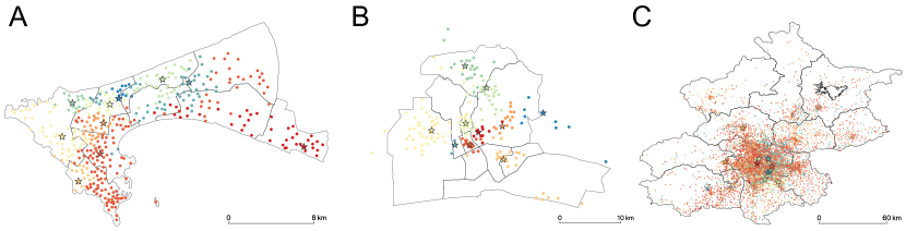
Figure 4: The community structure detected by our LS algorithm on mobility flow networks in three diversified cities across continents. (A) Dakar in Senegal, Africa. (B) Abidjan in Côte d’Ivoire, Africa. (C) Beijing in China, Asia. Each dot represents a location, which corresponds to a region by Voronoi tessellation according to cellphone towers. Communities are indicated by different colors, and their centers are marked as stars. The decision graphs are shown in Fig. S7.

Clustering vector data via the LS algorithm

Community detection and vector data clustering share many similarities, but are often considered separately and having contrasting focus. Our use of local leaders identified by local dominance was directly inspired by the concept of the center of a cluster, which is characterised by a higher centrality measure in its vicinity/neighborhood (e.g., density or degree) and a relatively long distance (i.e., a large $l_{i}$) to the nearest object with a large centrality. Local dominance concretely and explicitly identifies fundamental asymmetric leader-follower relation between objects, which naturally give rises to centers. This creates a direct link between the two viewpoints of network science and data science. It is therefore natural to ask whether LS would perform well, or even better, than vector data clustering methods on a discretised version of a data cloud.

To cluster vector data with the LS method, we first need to discretise it into a network. Many methods exist to perform this task, including $\epsilon$-ball, k-nearest-neighbors (kNN) and its variants (such as mutual kNN, continuous kNN), relaxed maximum spanning tree [64], percolation or threshold related methods [65, 35], and more sophisticated ones [66]. Here, we employ the commonly used $\epsilon$-ball method that sets a distance threshold $\epsilon$ and connects vectors, which become nodes, whose $\epsilon$-balls overlap, see Fig. 5A and inset. This process can be accelerated by using R-trees and are implemented in a time complexity of O($N\log N$) [67, 63] (see Supplementary Text A.4). After traversing all nodes, a network encoding a geometric closeness within $\epsilon$ between nodes is obtained, see Fig. 5B. The $\epsilon$-ball method preserves spatially local information, e.g., the vector density in the metric space can be interpreted as degree in the constructed network, and coarse-grains continuous distance between objects into discrete values. This makes the determination of centers clearer (see Fig. 5C and D). The choice of $\epsilon$ influences greatly the structure of the network obtained, here we chose $\epsilon$ to be near the network percolation value to ensure a minimally connected graph [68, 69, 70], more details on determining $\varepsilon$ can be found in Supplementary Text C.1.

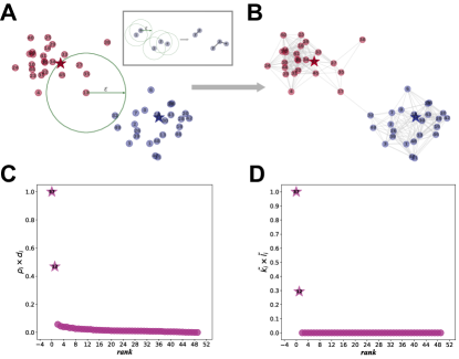
Figure 5: Conversion from vector data to a network via the $\varepsilon$-ball method and the analogy between the community centers of networks and the cluster centers of vector data. (A) An example of data cloud and (B) its dicretised network representation by (Inset) the $\varepsilon$-ball method. (C) The decision graph by the density and distance based (DDB) algorithm [16]. (D) The decision graph by the LS method. Cluster centers are data points of both a higher density $\rho_{i}$ than its neighbors and relatively far from other points with a larger density (i.e., a large $d_{i}$) [16]. The density $\rho_{i}$ of a data point $i$ is simply the number of nodes within a certain radius $\epsilon$, and it is equivalent to the degree of node $i$ in the corresponding network (i.e., $k_{i}=\rho_{i}$). The network constructing process is a coarse-graining and discretization process, where the absolute distance value is not preserved (e.g., in the Inset, $d_{32}>d_{34}$ for the original vector data, but $l_{32}=l_{34}=1$ in the network). The Euclidean distance between any data points is based on a global metric, but the topological path length between two nodes are based on a local metric. For example, $d_{24}$ is only slightly larger than $d_{34}$, but in the network, $l_{24}=2$ and $l_{23}=1$ (see the Inset); though $d_{21}\approx 2d_{23}$ according to global metric, node $2$ and node $1$ are not reachable in the network based on the local metric. Cluster centers identified by the DDB algorithm matches community centers identified by the LS method, which are all marked as stars.

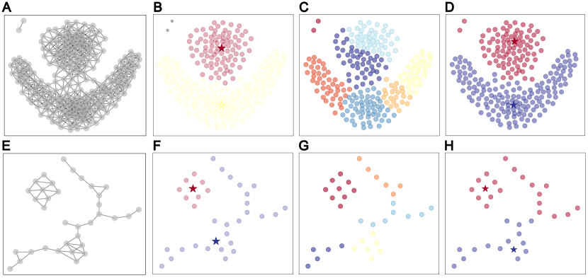
Figure 6: Comparisons on the clustering performance between the LS, Louvain, and DDB algorithms for two dimensional benchmark vector data. (A) and (E) represent networks constructed from vector data using the $\varepsilon$-ball method (see Supplementary Text C.1 and Fig. S10 for details on the network constructions). (B) and (F) show the result of the LS method that correctly identify clusters that align with common consensus (see Fig. S11 for more cases). In addition, LS can detect noisy points (marked in grey) that are of low degrees but long $l_{i}$. (C) and (E) show the partitions obtained from the Louvain method which are more fragmented than the LS results (see Fig. S13 for more cases). (D and H) show the results obtained from the DDB method which provides correct partitions to most benchmark data, see (D) and Ref. [16] for other cases, but fails in the test case in (E), where both a low density manifold and a high density cluster exist, due to its local association rule [71] being affected by a mixture of local and global metrics. LS and Louvain methods are performed on the constructed networks shown in A and E, and the DDB algorithm is performed on the original vector data.

Applying the LS algorithm on the constructed network for a series of well-known two dimensional benchmark data (Fig. 5A and E), yields the expected clusters (Fig. 5B and F, and Fig. S11 for more cases). By contrast, the Louvain algorithm generally obtains more and smaller clusters in a relatively fragmented way (Fig. 5C and G, and Fig. S13 for more examples) on the same networks. The reason is that the Louvain algorithm overlook the transitivity of local relations [72]. The state-of-the-art unsupervised clustering algorithm density and distance based (DDB) [16] applied to the original vector data yields expected clusters in most cases, see Fig. 6D and Ref. [16] for other examples. This confirms the universality of local hierarchy between objects and the analogy between our community centers and cluster centers. However, the DDB algorithm fails in the test case [71] in Fig. 6H due to a mixture of local and global metrics in this associate rule [71], which do not affect the LS method works (see Fig. 6F). From a network perspective, certain dynamics can give rise to meaningful clusters with arbitrary shapes in metric space (e.g., synchronization or spreading dynamics are usually only possible along the manifold via local interactions but not through global ones). For example, different clusters in Fig. 6E or Fig. S11C,G,H might correspond to groups of fireflies that are only able to synchronize within the group rather than between groups, as their interaction range is usually limited. In the situations above, the distance measured by the local metric is more appropriate than the one measured by the global metric, see a more in depth discussion in Supplementary Text C.2. The good performance of the LS algorithm on vector data resides in the correct identification of the local dominance, i.e., finding the centres, from the local metric.

In addition, we show that the LS method is robust against noisy data in different scenarios, see Supplementary Text D.1 and Figs. S23-S24. Though less common when considering vector data, targeted addition of edges in a network that connect two cluster centers, explicitly brings two cluster centers closer to each other in the metric space and will distort the space, whereas, conversely, the removal of links increases the distances between two objects.

The advantage of building networks for high dimensional vector data

We now show that the combination of the $\epsilon$-ball discretisation and LS community detection method also yields excellent results on high-dimensional data sets. We again use very high dimensional well-known benchmark: the MNIST of hand written digits [73], and Olivetti of human faces [74], and show that our simple framework outperforms the-state-of-the-art DDB clustering algorithm [16], see Table 2. Let us consider, for example, the Olivetti human face dataset, a challenging high dimensional dataset with small sample size. Each cluster obtained by the LS algorithm only contain images from a single individual, see Figs. S17-19, simply based on Euclidean distance between images and without resorting to using complex image similarity measure. Moreover, it obtains a higher $F_{1}$-score than the DDB method. We note that for MNIST and Olivetti datasets, the Louvain algorithm has a higher $F_{1}$-score than LS, but identifies an inappropriately large number of clusters. The better performance of the Louvain algorithm lies in some subtle differences from clustering results obtained by the LS method (see comparisons between Fig. S19A and Fig. S19B for the Olivetti dataset with 100 images. The Louvain algorithm detects all images of the eighth person as one cluster, but the LS method classifies four images of the eighth person as another cluster).

We conjecture that the conversion from vector data to a network is not merely a translation of the data, but a fundamental information filtering process that accentuates the prominence of local leaders and thus increases the strength of local hierarchy, which in practice turns out to be of great advantage to our framework for handling vector data with high dimensions. Constructing the network via $\epsilon$-balls is similar to a coarse-graining process: as long as two objects are close enough, the small differences in distances within $\epsilon$ are neglected. In addition, such a process also corresponds to subtracting irrelevant global information and puts the focus on similarity based on a local metric. Though there will be some information loss during the conversion from vector data to topological data, purely local information is enough to identify local dominance in the data. Not all information embedded in the vector data needs be utilized [64], sometimes too much information might complicate the process. Although admitting asymmetric relations between objects would violate certain formal metric properties (distances are symmetric), it turns out to be an advantage for cluster analysis (see more discussions in Supplementary Text C).

	$D$	$N$	$N_{c}$	LS		DDB		Louvain
				$F_{1}$	$N_{c}$	$F_{1}$	$N_{c}$	$F_{1}$	$N_{c}$
Iris	4	50	3	0.73	2	0.82	3	0.70	8
Wine	13	178	3	0.57	3	0.57	3	0.41	7
MNIST	784	1,000	10	0.32	21	0.26	(10)	0.45	247
Olivetti	10,304	100	10	0.74	14	0.64	(10)	0.78	32
Olivetti	10,304	400	40	0.59	64	0.49	(40)	0.68	112

Table 2: Comparisons on the clustering performance between the LS, Louvain, and DDB algorithms for high dimensional vector data. $D$ denotes the dimension of the dataset, $N$ denotes the number of objects, and $N_{c}$ denotes the number of clusters from the ground-truth or identified from algorithms. The hand-written figures in MNIST is of dimension 28$\times$28=784 pixels; and in Olivetti, the face image is of dimension 92$\times$112=10,304 pixels. The Olivetti dataset with $N$=100 comprises the first 100 images of 10 people from the original data set. The original dataset comprises 400 images of 40 different people. Our LS algorithm outperforms DDB in all high-dimensional and large-scale data sets except in Iris, whose dimension is quite low. Note that as the DDB algorithm does not have a clear recognition of the number of clusters (i.e., no clear gaps between centres in the decision graph) [16] for MNIST and Olivetti, the number of clusters identified by DDB are putative based on the ground truth (i.e., selecting the top ten or forty nodes in the decision graph), which is marked in brackets. Digits highlight in bold is the ones closest to the ground truth among all three algorithms.

DISCUSSION

Community detection and cluster analysis are analogous as both aim to group objects into categories based on some notion of similarity. In this work, we develop a fast and scalable community detection method based on the notion of a community center which echoes the commonly used concept of a cluster center. The identification of community and cluster structures requires a heterogeneous system: uniformly distributed data points and strictly regular networks do not possess meaningful mesoscopic cluster structure. Heterogeneity leads to the emergence of more important loci in a data space, or central nodes in a network. The notion of centre is pervasive in cluster analysis, but underused in community detection. We define community centres as local leaders that are both of a high degree, corresponding to a high density in cluster analysis, and relatively distant from other local leaders, corresponding to cluster separability. The nodes belonging to each community defined by their centre are identified by basins of attraction[34] based on the dominance existing between nodes, which indicates the asymmetric leader-follower relationship and defines a local hierarchy. While dominance is an explicit characteristic of edges in a directed network, it can be seen as an intrinsic higher-order directionality between nodes in undirected networks. The resulting local hierarchy reflects asymmetric interactions between objects inferred from the local connectivity of nodes that then naturally defines leaders and community affiliations. In addition, local hierarchy can be treated as an intrinsic property of the network.

The local hierarchy structure is quite robust against random noise, and is based on local information. Moreover, in contrast with most state-of-the-art clustering and community detection methods, the LS method does not rely on a global objective function to optimise based on a null model nor is it dependent on dynamical processes. In cluster analysis, approximating similarity relations between objects by a distance matrix actually assumes that every object are in a direct relation with all others, which is also the case for modularity optimization algorithm that utilize a random null model, which also assumes that each node has a probability to interact with every other node [10]. In addition, community detection methods also generally assume a mutual relation between objects, which is an important formal metric property and an implicit feature of an undirected connectivity matrix. Local hierarchy implicitly violates such an assumption, but it turns out that abandoning such a restriction gives better flexibility to the clustering method (see Supplementary Text C for more details). Finally, our LS algorithm is fast and scalable with a linear time complexity and also performs well on most benchmarks, except the ones that do not possess the type of heterogeneity exploited by LS.

Overall, the performance of the LS method is particularly good given its simplicity. On benchmark network models, it outperforms the currently most widely used community detection method, the Louvain modularity optimisation algorithm. The LS method consistently ranks higher than any other methods when the performance is averaged over several data sets, see Table S2. We have also shown that the LS method is naturally able to detect multiscale structure of communities in complex networks. This implies that while not necessarily identifying the partition defined by some existing ground truth, it finds a good approximation of it and the output can then be used as starting point for other slower but more accurate and dedicated community detection methods, offering a significant speed up.

Given the similarity in spirit between LS and clustering methods, we applied LS to $\epsilon$-ball discretised version of benchmark vector data, both low and high dimensional. For low-dimensional data, we find it provides the expected clusters and outperforms Louvain modularity optimisation algorithm ran on the discretised data, which generally yields too many communities. LS also outperforms DDB, a state-of-the-art unsupervised clustering method, on some challenging cases in the presence of low-density manifolds. For high-dimensional data, LS still outperforms DDB, but not Louvain, although on closer inspection, Louvain obtains a better $F_{1}$-score, but suffers again from providing too many communities, outbalancing the advantage in $F_{1}$-score.

We hypothesise that the discretisation step of creating a network from vector data acts as a topological filter, which enhances the key property of the data that makes cluster detection work: the existence of well defined cluster centers and a clearer identification of local hierarchy. The performance of any community detection algorithm is going to be influenced by the discretisation method used, and more work is needed to understand the relationship between topological denoising and the performance of the community detection algorithms, as different community detection methods might respond differently to different discretisation schemes.

Another area for future work is to adapt LS to find “halo” nodes residing at the boundary of two or more communities (e.g., node d in Fig. 1), detect overlapping communities [13] potentially by producing line graphs [75, 76, 77] or clique graphs [49], and identify critical link responsible for the merging or splitting dynamics of communities [51]. Another point that could be improved is when two or more local leaders are equivalent on both degree and distance to a node. We currently assign it to a local leaders at random but we could look at other options.

Finally, another possible direction for future research concerns the definition of dominance itself. In this article, it was built on a specific network property, the degrees of the nodes. For a weighted network, it would be appropriate to use strength rather than degree and we would retain all the benefits of the LS method. Dominance could also be based on other node centrality measures but most of these require global network calculations which would slow the algorithm considerably. If Dominance was based on non-structural properties, such as numerical attributes for nodes already defined in the data, then the LS approach would still work well.

SUPPLEMENTARY MATERIALS

Supplementary material for this article is available at

Supplementary Text

tables S1 - S2

figs. S1 - S27

References

REFERENCES AND NOTES

Acknowledgements: R.Li acknowledges helpful discussions with Dr. Gezhi Xiu and Dr. Wenyi Fang from Peking University. F.S. acknowledges technical help from Mr. Ankang Luo and Ms. Chenxin Liu from UrbanNet Lab. Funding: This work receives financial supports from the National Natural Science Foundation of China (Grant No. 61903020), Fundamental Research Funds for the Central Universities (Grant No. buctrc201825). L.L. acknowledges the financial supports from the XPLORER PRIZE, and the Special Project for the Central Guidance on Local Science and Technology Development of Sichuan Province (Grant No. 2021ZYD0029). R.L. acknowledges support from the EPSRC Grants EP/V013068/1 and EP/V03474X/1. Author contributions: R.Li conceived the research. R.Li, B.C., H.E.S., L.L., P.E., T.E, and R.L. designed the research. R.Li and F.S. designed the first version of the LS algorithm, T.E. further refined and improved the algorithm. F.S. implemented the LS algorithm and conducted experiments. A.Y. conducted some auxiliary experiments. R.Li, F.S., B.C., P.E., L.L., T.E. and R.L. discussed the results and wrote the manuscript. R.Li was the lead writer of earlier versions of the manuscript. All authors reviewed the manuscript. Competing interests: The authors declare that they have no competing interests. Data and materials availability: All network and vector datasets needed to evaluate the conclusions in the paper are publicly available and present in the paper and/or the Supplementary Materials. The original cellphone datasets of Dakar and Abidjan are accessed through the D4D challenge, and the Beijing dataset is obtained from a Chinese telecommunication operator and the original dataset is not publicly available. Computer code for the LS algorithm and code implementing the analysis described in this paper and other information can be found online at https://github.com/UrbanNet-Lab/LS_for_CommunityDetection_and_Clustering.

Supplementary Materials for
Local dominance unveils clusters in networks

Supplementary Text A   The Local Search (LS) algorithm

A.1 Identification of local leaders

As mentioned in the main text, when there are multiple nearest nodes of a larger or equal degree than the ego node $i$, then $i$ will first point to all of them. Then, after traversing all nodes, for each node we keep one out-going edge, chosen at random, which destroys any loops (see Lemma 1 and Fig. S1C) and gives us a tree. Such a setting gives good partitions even for some extreme cases (e.g., a lattice or clique).

A.1.1 Strictly homogeneous networks

When there is a complete subgraph in the neighborhood of a node (see Fig. S1A), the mapping of local dominance can vary (see Fig. S1B) due to randomness, but the different mappings all have the same eventual partition. In a lattice network, following the same process of the LS algorithm, the whole network will be classified into just one community.

Lemma 1

No formation of loops by the LS algorithm. The mapping in Fig. S1C is impossible.
Proof: If $a\rightarrow b$, $b\rightarrow c$, and $c\rightarrow d$, then it means that $k_{d}\geq k_{c}\geq k_{b}\geq k_{a}$. Now, if $d\rightarrow a$, it indicates $k_{a}\geq k_{d}$, then we have $k_{a}=k_{b}=k_{c}=k_{d}$ and $A_{ad}=1$. But if so, given $A_{ad}=1$ and $k_{a}=k_{d}$, then as a is first traversed, there will be a $a\rightarrow d$ instead of $d\rightarrow a$, and eventually, a will only keep one out-going link, thus no such loop shown in C will be formed. $\blacksquare$

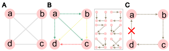
Fig. S1: The mapping of local dominance in a complete network. (A) The structure of a complete graph, and here we assume that nodes will be traversed from a to d in order (any other orders for the nodes lead to the same result). (B) Node a will first point to all three other nodes as $k_{j}\geq k_{a}$, then node b will point to c and d but not a (as a is already a possible follower of b), then c will point to d (but not a and b, as they are also possible followers of c), and d points to no one as there is no remaining neighbor with $k_{j}\geq k_{d}$. Then we randomly keep only one out-going link for each node. For example, b can either point to c or d with an equal probability. The eventual mapping of local dominance can be either a chain or a star in two extremes. For such a 4-clique, there are 6 possible mappings (see the Inset on the right), and all of them yield just one community. (C) No such a loop will be formed, see proof of the Lemma 1.

A.1.2 Relatively homogeneous ER random networks

In relatively homogeneous networks (e.g., ER random networks), degree differences exist, and communities may emerge. In such networks, large degree nodes often have a relatively higher probability connecting to each other, which will lead to fewer local leaders and eventually fewer communities. In the thermodynamic limit, an ER network is regarded as having no community structure (or the whole network should be classified into one community) due to a strong homogeneity. When implementing the LS and Louvain algorithm on ER networks, the LS method obtains fewer communities, which is closer to the common assumption (see Fig. S2).

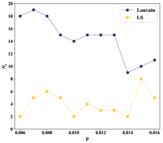
Fig. S2: The number of communities detected by the Louvain and LS methods in ER random networks with $N=1000$. The LS method detects fewer communities than the Louvain algorithm. For ER random networks with 10,000 nodes and $p$ equals 0.001, the LS method ends up with 15 communities and the Louvain with 22 communities.

For random networks generated by stochastic block model (SBM) [40, 41] that comprise two communities, each of which are of 1,000 nodes (i.e., $N=2000$) with intra-connection probability $c_{in}=0.009$, when the inter-connection probability $c_{out}=0$, the LS algorithm detects 9 communities and the Louvain algorithm detects two communities. The result obtained by the Louvain algorithm aligns with ground truth, but also reflects the resolution limit [44], and in contrast, the LS algorithm still detects as many as community centers as when looking at each individual ER network. When we fix $c_{in}$ and gradually increase $c_{out}$, the $F_{1}$-score of the LS algorithm is roughly around 0.4, while the Louvain algorithm has a fast decrease, which is mainly influenced by internal connections and the number of communities detected.

A.1.3 Heterogeneous Ravasz-Barabási networks

In a classical Ravasz-Barabási networks (see Fig. S4A) that exhibits strong heterogeneity, we can easily identify local leaders and followers. Nodes b, c, d, and e (with $k_{i}=20$, $l_{i}=2$) are identified as local leaders by the LS algorithm (see Fig. S4C), as they are of a larger degree than all their neighbors (other neighbors are of a degree $k_{i}\in[3,5]$) and are relatively far away from a larger node (here, only the central node a is of a larger degree ($k_{a}=84$) and is two steps away from them). For example, those four nodes surrounding c are not connected to node a, thus they point to c, but other nodes in the four 2-level peripheral clusters (e.g., those four clusters surrounding the cluster centered at c) are all also directly connected to the central node a, as $k_{a}>k_{c}$ and $d_{ia}=d_{ic}=1$, thus those nodes all point to a and are eventually partitioned to the community centered at a. As for the Louvain algorithm, the partition results strongly depend on the traversal sequence, and it maximizes modularity in a greedy way if the modularity gain $\Delta M_{c_{i}c_{j}}$ is positive.

$$\Delta M_{c_{i}c_{j}}=\frac{1}{E}\left(E_{c_{i}c_{j}}-\frac{k_{c_{i}}k_{c_{j}}}{2E}\right),$$ (1)

where $E$ is the number of edges in the network ($E=344$ in the Ravasz-Barabási network in Fig. S4A), $E_{c_{i}c_{j}}$ is the number of edges that connect nodes in community $c_{i}$ and community $c_{j}$, and $k_{c_{i}}$ denotes the sum of degree of all nodes in community $i$. For example, as shown in Fig. 2F in the main text, the small cluster (denote as $c_{1}$) will not be merged to the purple one (denote as $c_{2}$), as $E_{c_{1}c_{2}}=4$, and $k_{c_{1}}=4\times 5=20$, $k_{c_{2}}=84+3\times 4+4\times 5\times 3=156$, in this case, $\Delta M_{c_{1}c_{2}}<0$, and these two communities will not be merged together.

When we further modify the network in Fig. S4A to add a 3-level branching to the top-right 2-level cluster centered at b (see Fig. S4B), then the degree of node b become the same as the original central node a (i.e., $k_{a}=k_{b}=84$). As all those four 2-level peripheral clusters surrounding node b are both connected to both a and b, thus, they will eventually point to one of them at random (in this realization, there are seven nodes point to a and eventually colored as purple, and the remaining nodes point to b and colored as blue). Again, due to the same reason as in Fig. S4A, four smaller new communities emerge, which are centered at nodes f, g, h, and i, respectively (see Fig. S4D). As we remove 4 links from node d, and 8 links from node e, thus $k_{d}=16$ and $k_{e}=12$, and this is why in the decision graph in Fig. S4D, nodes d and e drops a little bit each. In addition, the decision graph can also make meaningful ranking for community centers (see Fig. S4D). The network can be partitioned into nine communities at the finest resolution (see Fig. S4B), or into two big communities (small communities centered at c, d, and e will follow a, and other four small communities follow b as a is more further away from them), which reswembles a multiscale community structure.

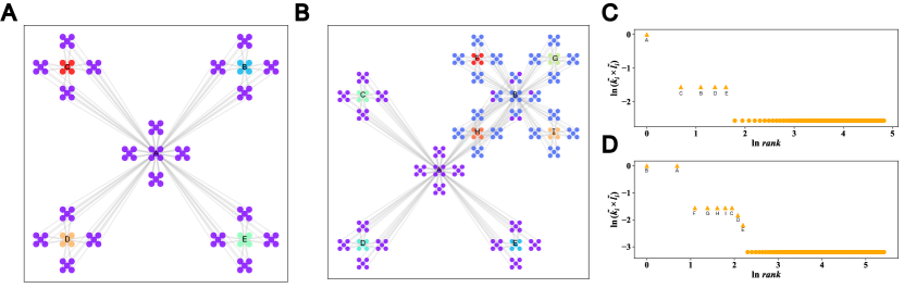
Fig. S4: The community partitions by the LS algorithm on Ravasz-Barabási networks. (A) A 2-level Ravasz-Barabási network [43], where four small communities identified by the LS method. The color correspond to community partitions. (B) A modified Ravasz-Barabási with the top-right 2-level cluster with 3-level branching. For the bottom-left 2-level cluster, we remove four links; and for the bottom-right 2-level cluster, we remove eight links. (C) The decision graph for the network in A by the LS algorithm. (D) The decision graph for the network in B by the LS algorithm.

A.1.4 Multiscale community structure

To further verify the impacts of homogeneity on the LS method for detecting multiscale community structure, we obtain the degree frequency distribution for the scale-free setting (see Fig. 3A in the main text and Fig. S5A for its degree distribution) and the random setting (see Fig. 3B in the main text and Fig. S5B). Though the maximal degree in the random setting is smaller than in the scale-free setting, but there are more nodes beyond the reference value in the random setting (red line in the figure, i.e., the smallest degree value among the largest nodes in each of sixteen communities). In the random setting (see Fig. S5B), for a largest node in a ground-truth community that is of a degree near the reference value, there are more nodes with a larger degree out there in the network, and it will have a relatively higher probability to connect to one of them. If this happens, this largest degree node in the ground-truth community will be diminished as a follower, and the corresponding community cannot be detected. In contrast, in the scale-free setting in Fig. S5A, there are fewer larger nodes and thus a smaller chance of direct connections between them. In addition, in the random setting in Fig. S5B, a small decrease of the reference value will lead to a large increase on the number of nodes beyond it. While in the scale-free setting (see Fig. S5A), small fluctuations to the reference value would have a much milder influence. This explains that why the LS algorithm works better on the scale-free setting on detecting multiscale community structure than in the random setting (see Fig. 3 in the main text).

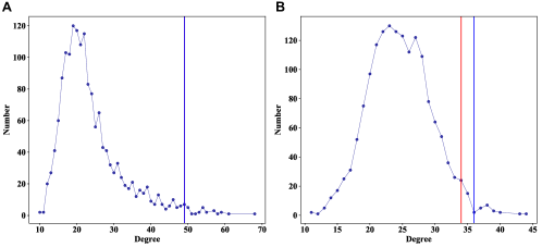
Fig. S5: The degree frequency distribution of multiscale networks. (A) The scale-free setting (i.e., each second level community is a scale-free network). The whole network is still of a heterogeneous degree distribution. (B) The random setting (i.e., each second level community is a ER random network). The degree distribution is relatively homogeneous. Networks in A and B are of the same average degree. The red line indicates the smallest value of all of the largest node in each of all sixteen ground-truth communities, and this value is what we called “reference value” in the main text. And the blue line indicates the smallest value of centers of all identified communities. In A, these two lines overlap; while in B, the blue line is larger than the reference value, which also indicates that some clusters are.

A.2 Identification of community centers

For better clarity and later use, we define $\mathbf{C}$ as the set of all local leaders (i.e., potential community centers), and $\mathbf{M}$ as a subset of local leaders that are of the maximal degree in the network (i.e., $\mathbf{M\subseteq C}$). It is worth noting that not all nodes with the maximal degree in the network will be in the set of $\mathbf{M}$. For example, in Fig. 1C in the main text, nodes m, f, and p are in the set $\mathbf{C}$, and node m in the set $\mathbf{M}$ as it is of the maximal degree in the whole network and is a local leader. In contrast, though the node b is also of the maximal degree in the whole network, it is not in $\mathbf{M}$ or $\mathbf{C}$ as it already follows node m and is not identified as a local leader. In the Football network [8, 49, 50], there are several nodes with the maximal degree are not in $\mathbf{M}$ (see those nodes with a degree equal 12 at the right-bottom of Fig. S7A).

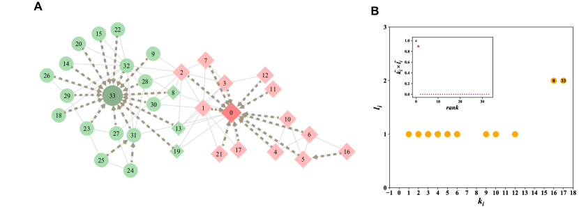
Fig. S6: The community detection result by the LS algorithm on the Zachary Karate Club network. (A) The shape of the node represents the ground-truth community label, where the circle represents one group and the square represents the other. The color of the node represents the predicted labels by the LS algorithm. Zachary [39] identifies two social groups, one led by the instructor, node 0, and the other led by the club president, node 33 (the node index here is one less than that used in [39]). These nodes are correctly identified as community centers by the LS method. Nodes 8, 13, and 19 are connected to both centers and eventually classified to the community centered at the club president (node 33) due to a slight degree difference between two centers ($k_{33}=17>k_{0}=16$). Out-going links $i\rightarrow j$ indicates that node $j$ dominates node $i$. (B) The scatter plot of degree $k_{i}$ and path length $l_{i}$ for all nodes. Community centers are identified as the ones with both a larger $k_{i}$ and $l_{i}$. (Inset) The decision graph for quantitatively determining community centers (indicated by triangles) based on the product of rescaled degree $\tilde{k}_{i}$ and rescaled distance $\tilde{l}_{i}$. Community centers can be determined by a visual inspection for a big gap or by more sophisticated automatic detection methods.

For each node $i$, finding a nearest node $j$ with a largest degree and $k_{j}\geq k_{i}$ can give rise to a field of hidden directionality $(i\rightarrow j)$ on networks as shown in Fig. 1C in the main text and Fig. S6A. We denote the length of the shortest-path from $i$ to $j$ as $l_{i}$, and there will be at most one out-going link for each node. The degree $k_{i}$ and path length $l_{i}$ can provide effective information for determining community centers, which are nodes with both a larger $k_{i}$ and $l_{i}$ (see Fig. 1E in the main text, Fig. S6B, and Figs. S7-S8).

As most real networks are scale-free with a power-law distribution on degree, to reduce the impacts of extreme degree values caused by hub nodes, we calculate a ranked degree

$$k_{i}^{*}=\mathrm{rank}(k_{i}),$$ (2)

where the $\mathrm{rank}()$ function returns the index of a value in the ascendingly sorted set. The node(s) with the smallest degree will (all) have $k_{i}^{*}=1$ regardless of its specific degree value $k_{i}$, and the node(s) with the largest degree will have $k_{i}^{*}=len(set(k_{i}))$, where $set(k_{i})$ returns all unique degree values of all nodes in the network, and $len()$ is a function calculating the length of the set. For example, for a network with degree values as $(1,1,1,3,3,3,6)$, the corresponding $k_{i}^{*}$ will be $[1,1,1,2,2,2,3]$. So, in this case, when $k_{i}=6$, $k_{i}^{*}=3$. Meanwhile, in order to ensure that the shortest-path length differences are more distinguishable, we calculate a rescaled path length

$$l_{i}^{*}=l_{i}^{2}.$$ (3)

Note that most networks generated from 2D benchmark vector data (see Fig. S12) are of a relatively narrow degree distribution, in such cases, $k_{i}^{*}$ is quite comparable with $k_{i}$, and $l_{i}$ is also relatively more distinguishable (see Fig. S12). Thus, in those cases, $k_{i}$ and $l_{i}$ can already have a quite comparable performance as of $k_{i}^{*}$ and $l_{i}^{*}$. One practical reason is that the density is quite comparable across different clusters in most benchmark 2D vector data sets [78, 79, 80, 81]. When the density is more heterogeneous across clusters, the degree distribution might be closer to a power-law and then the operation of calculating $k_{i}^{*}$ will be necessary.

To make $k_{i}^{*}$ and $l_{i}^{*}$ more comparable on magnitudes, we do a min-max normalization for them.

$$\tilde{k}_{i}=\frac{k_{i}^{*}-\min(k_{i}^{*})}{\max(k_{i}^{*})-\min(k_{i}^{*})},\ \ \ \tilde{l}_{i}=\frac{l_{i}^{*}-\min(l_{i}^{*})}{\max(l_{i}^{*})-\min(l_{i}^{*})}.$$ (4)

The number of community centers can be easily identified according to the rank distribution of $\tilde{k}_{i}\times\tilde{l}_{i}$, which is a composite indicator on the centerness of a node. Generally, there will be a gap between community centers and other nodes (see Fig. S6B and insets of Fig. S7), which can be better visually inspected in a log-log plot (see insets of Fig. S7D-F).

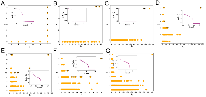
Fig. S7: Identification of community centers of real networks. Scatter plots of $k_{i}$ and $l_{i}$ for (A) Football [8, 49, 50], (B) Polbooks [82], (C) Polblogs [52], (D) Cora [83], (E) Citeseers [84], (F) Pubmed [85], and (G) DBLP [48]. (Insets) Decision graph for quantitatively determining community centers based on the product of ${\tilde{k}_{i}}$ and ${\tilde{l}_{i}}$. Identified community centers are highlighted by larger triangles.

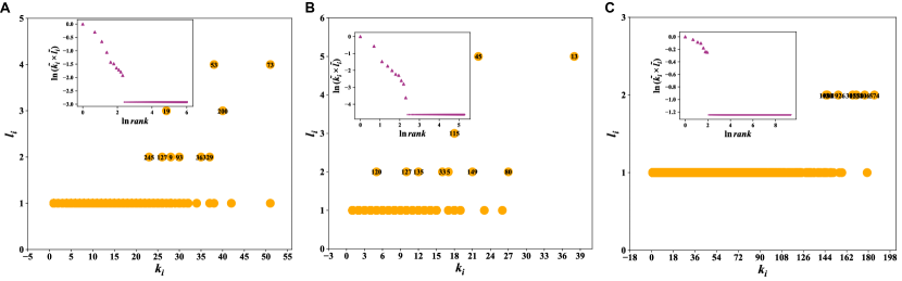
Fig. S8: Identification of community centers of human mobility flow networks in three diversified cities. (A) Dakar in Senegal, Africa. (B) Abidjan in Côte d’Ivoire, Africa. (C) Beijing in China, Asia. Identified cluster centers are highlighted by larger triangles.

A.3 Pseudo Code of our LS algorithm

Input: $G=(V,E)$: undirected and unweighted graph, where $V$ is the set of vertices, and $E$ is the set of edges.

Output: Community partitions.

1

2for node i $\mathbf{in}$ V do

3       $j$ = node with the maximum degree in neighborhood of $i$;

4       if $k_{j}\geq k_{i}$ then

5             $i\rightarrow j$;

6            $l_{i}=1$;

7            

8       end if

9      

10 end for

11Build DAGs by $directionality(i\rightarrow j)$, and obtain $\mathbf{C}$ and $\mathbf{M}$;

12   #$\mathbf{C}$ is the set of nodes with no outgoing edges in DAGs;

13   #$\mathbf{M}$ is the set of node(s) with the maximum degree in $\mathbf{C}$;

14 for node i $\mathbf{in}$ $\mathbf{C}\backslash\mathbf{M}$ do

15       $m$ = 2;

16       Perform a $local$-$BFS(G,\ i)$ to find $m$-order neighborhood of $i$;

17       $j$ = node with the maximum degree in $m$-order neighborhood;

18       if $k_{j}\geq k_{i}$ then

19             $i\rightarrow j$;

20            $l_{i}=d_{ij}$;

21             continue;

22            

23      else

24            m += 1;

25             go to line 13;

26       end if

27      

28 end for

29for node i $\mathbf{in}$ $M$ do

30       $l_{i}=max(l_{k}),\ \forall k\in V$;

31      

32 end for

33for node i $\mathbf{in}$ $C$ do

34       $\delta_{i}=\tilde{l}_{i}\times\tilde{k}_{i}$;    # $\tilde{l}_{i}$ and $\tilde{k}_{i}$ are calculated according to Eq.(3).

35 end for

36

37Determine the $community\ centers$ according to descendingly sorted $\delta_{i}$;

38

39Assign community labels from $community\ centers$ to their neighbors along the reverse direction $i\leftarrow j$ of hidden directionality ($i\rightarrow j$);

return partitioned sets of nodes according to community labels

Algorithm 1 The Local Search (LS) algorithm for community detection

A.4 Time Complexity

	$N$	$E$	$|\mathbf{C}|$	$\langle k\rangle$	$\langle l\rangle$	${\langle l\rangle}_{\mathbf{C\backslash M}}$	$(|\mathbf{C}|-|\mathbf{M}|)\langle k\rangle^{\langle l\rangle_{\mathbf{C\backslash M}}}$
Karate [39]	34	78	2	4.59	1.058	2.00	21.05
Football [8, 49, 50]	115	613	6	10.66	1.069	–	–
Polbooks [82]	105	441	2	8.40	1.057	4.00	4978.71 (441)
Polblogs [52]	1,222	16,717	3	27.36	1.002	2.00	1,497.15
Cora [83]	2,485	5,069	104	4.08	1.047	2.16	2,132.77
Citeseers [84]	2,110	3,668	106	3.48	1.080	2.76	3279.96
PubMed [85]	19,717	44,327	472	4.50	1.025	2.06	10,445.59

Table S1: Basic statistics on real networks with ground-truth community labels and intermediate results of the LS algorithm. $N$ is the number of nodes in the network, $E$ is the number of edges, $|\mathbf{C}|$ is the size of the set of potential centers (i.e., local leaders) identified by our LS algorithm, $\langle k\rangle$ is the average degree of the network, $\langle l\rangle=\sum_{i}l_{i}$ is the average number of layers searched when a node finds a nearest node with a larger or equal degree than itself, $\langle l\rangle_{\mathbf{C}\backslash\mathbf{M}}$ is the average number of layers searched for all potential centers except the local leader(s) in $\mathbf{M}$ with the maximal degree in the whole network (i.e., $i\in\mathbf{C}\backslash\mathbf{M}$), thus $(|\mathbf{C}|-|\mathbf{M}|)\langle k\rangle^{\langle l\rangle_{\mathbf{C}\backslash\mathbf{M}}}$ is the theoretical average number of links need to be traversed by the LS algorithm, which is bounded by $(|\mathbf{C}|-|\mathbf{M}|)E$ and is usually smaller than $E$. In most cases, there will be only one or very a few nodes in $\mathbf{M}$. For example, in Polbooks, there is one node in $\mathbf{M}$, thus $\langle l\rangle_{\mathbf{c}\backslash\mathbf{M}}$ reflects the length of shortest-path between the secondary potential center and the first potential center. The shortest path length is 4 and the calculation based on $(|\mathbf{C}|-|\mathbf{M}|)\langle k\rangle^{\langle l\rangle_{\mathbf{C\backslash M}}}$ is 4978.71, however, it is at most 441 in practice to traverse all edges (which is indicated in parentheses). In the Football network, we identify 6 potential centers, and they are all of the same maximal degree in the network, thus there is no need to perform local-BFS for any of them, and they are identified as centers. Thus we did not report the values in the last two columns of the Football network.

In the LS algorithm, for each local leader, we perform a local-BFS that will stop further searching when encountering a nearest local leader that is of a larger or equal degree. Based on empirical analysis on real networks, the average number of searching layers $\langle l\rangle_{\mathbf{C\backslash M}}$ is only slightly larger than 2 in most cases (see Table S1). For other follower nodes, they just need to traverse all their first-order neighbors. In addition, such a local-BFS, which is theoretically approximated by $\langle k\rangle^{\langle l\rangle_{\mathbf{C\backslash M}}}$, is bounded by the number of edges $E$ in the network, thus the maximal value of $(|\mathbf{C}|-|\mathbf{M}|)\langle k\rangle^{\langle l\rangle_{\mathbf{C\backslash M}}}$ is $(|\mathbf{C}|-|\mathbf{M}|)E$, which is usually acceptable, and is usually smaller than $E$ (see the last column of Table S1). It is worth noting that not all nodes with the maximal degree in the network will be in the set of $\mathbf{M}$, only those identified as local leaders and are of the maximal degree are. For example, if there are several nodes with the maximal degree and they are connected to each other (see Fig. S1A), then there will be only one node identified as a local leader (see Fig. S1B).

For clustering vector data, before performing our LS algorithm, the network construction process takes O($N\log_{b}N$) if accelerated by R-tree [67, 63], where $b$ is the branching factor of the R-tree. If this process is not accelerated by R-tree, the time complexity of this part would be O($N^{2}$), which calculates a full distance matrix. After the network is constructed, the remaining process is the same, detected communities correspond to cluster partitions.

Supplementary Text B   Evaluation on the performance of both community detection and cluster analysis by F1 score

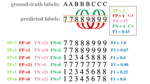
Fig. S9: The definition of TP, FP, TN and FN in evaluating grouping results. The objects within red boxes indicate that their true labels belong to the same communities. The objects in green boxes have the same ground-truth labels and predicted labels. The number of combinations of objects within each green box is the value of TP. The number of green arrows is FN, which corresponds to combinations of objects that are of the different predicted labels but the same ground-truth label. Likewise, the objects connected by red arrows have different ground-truth labels but the same predicted label, the number of which is FP (indicated by red arrows). TN is the number of objects that their true labels and predicted labels both belong to different communities. In the case of $(7,7,8,8,9,8,9,9)$, ${TN=2\times 3+2\times 3+2\times 2+1\times 1}$. Note that $TP+FP+TN+FN=C(n,2)$, where $n$ is the number of objects and $C(n,2)$ is the combination of choosing 2 out of $n$ objects. Thus when three of them are calculated, the other one can be calculated in this way, e.g., in the above example, $TN=C(8,2)-3-4-4=17$. The formula of $F_{1}$ is shown in Eq. (5). $F_{1}$ is in the range of $[0,1]$, when the difference between the predicted labels and the ground-truth labels is smaller, the $F_{1}$ score will be larger.

The performance of both community detection and cluster analysis can be evaluated by $F_{1}$-score that is defined as follows:

$$\begin{split}\mathrm{Precision}&=\frac{\mathrm{TP}}{\mathrm{TP}+\mathrm{FP}},\\ \mathrm{Recall}&=\frac{\mathrm{TP}}{\mathrm{TP}+\mathrm{FN}},\\ F_{1}\ &=\frac{2\times\mathrm{Precision}\times\mathrm{Recall}}{\mathrm{Precision}+\mathrm{Recall}}.\end{split}$$ (5)

TP is the number of combinations of nodes that are of the same predicted labels and the same ground-truth labels (see the combinations in green rectangles in Fig. S9). FP is the number of combinations of nodes that are of the same predicted labels but different ground-truth labels (see red curved arrows in Fig. S9). FN is the number of combinations of nodes that are of different predicted labels but the same ground-truth labels (see green curved arrows in Fig. S9). TN is the number of combinations of nodes that are of the different predicted labels and different ground-truth labels (see the calculation process in Fig. S9). Precision is the ratio of TP to the sum of TP and FP, which measures the fraction of correct (or positive) results among the predictions of the algorithm. The higher the precision, a larger fraction of combinations of nodes predicted in the same community are really in the same community according to the ground-truth labels. Recall is the ratio of TP to the sum of TP and FN, which measures the coverage of the positive predictions against the ground-truth positive set. The higher the Recall, a larger ratio of positive (or correct) combinations of nodes in the predicted community according to the ground-truth labels to the combinations of nodes in the same ground-truth community. However, Precision is strongly affected by the size of the predicted positive set, which means that precision can easily reach a high score if you only predict a tiny set of positive items that are highly probably positive, but then the coverage of positive items can be quite low. While, Recall can be one if you predict all items are positive, as it only measures the coverage of positive items. To be more comprehensive on both sides, $F_{1}$ takes the weighted harmonic average of Precision and Recall as its value, where the weights of them are usually set to be 1. The weight can be tuned by the different focus on either aspect. $F_{1}$ is in the range of $[0,1]$, a higher $F_{1}$ score indicates a better partition. In comparison, the normalized mutual information (NMI) is biased to smaller groups, i.e., when small communities are detected correctly, the NMI will increase more. And modularity only seeks for maximizing the difference between the partition and a global random null model [44], it can be blind to other generating process of networks in reality [27]. In networks constructed from vector data, some clusters may not corresponds to a high modularity value (e.g., networks constructed from some manifolds as shown in Fig. 4C,G,H in the main text). In flow networks, evidence indicates that the optimizing modularity might not lead to an optimal partition in some cases due to neglecting the structural regularity of interdependence characterized by flows [26]. Sometimes, a partition with the largest modularity is highly probably not the actual division of communities in real networks [44].

It is worth noting that although the evaluation of the classification performance of an algorithm with a ground truth is standard practice, the choice of the ground truth(s) are crucial. The ground truth of community partitions usually require detailed survey, which can be quite difficult for very large networks [41], and usually cannot be regarded as the same as metadata [41, 27]. For example, in the well known Zachary Karate Club network [39], the metadata of nodes can also be their gender, age, major, ethnicity, however, most of which are irrelevant to the community structure when interested in understanding the split of the club[41, 27]. In the DBLP collaboration network [48], where two authors are connected if they publish at least one paper together, the meta data of papers is the publication venue (i.e., journal or conference) which forms the basis of identifying communities in ref. [48] (i.e., authors who published to a certain journal or conference form a community), but the meta data is different from ground truth, if there is any. In some cases, meta data is related to community structure, but they two are not equivalent, otherwise, there is no need to do community detection based on topology but just look at meta data [41, 27]. For the Football network [8], we also used the ground truth labeling given by Evans [49, 50]. We calculate the $F_{1}$-score for all methods based on both sets (see Table S1), and we find that results obtained by most methods better align with the ones in refs. [49, 50], which is indicated by higher $F_{1}$-scores. As for the Polblogs network, there might be indeed three groups in it (i.e., apart from liberal and conservative, there is a neutral community) [52], which partially explains why the LS does not work that well on this example when compared with other examples, as LS detects three communities (see Table 1 in the main text).

	$\langle rank\rangle$	Karate	Football[8]	Football[50]	Polbooks	Polblogs	Cora	Citeseers	Pubmed	Time Complexity
GN [8]	4.9	0.59	0.60	0.84	0.80	0.74	0.32	0.23	0.18	O$(N^{3})$
Walktrap [86]	5.7	0.51	0.60	0.88	0.79	0.88	0.29	0.14	0.16	O$(N^{2}\log N)$
Spectral [23]	4.3	0.62	0.49	0.54	0.70	0.89	0.32	0.25	0.46	O$(N^{2}\log N)$
Spin glass [87]	4.9	0.61	0.60	0.92	0.62	0.88	0.33	0.22	0.21	NA
Fastgreedy [25]	3.3	0.75	0.55	0.56	0.78	0.89	0.39	0.28	0.32	O$(N\log N)$
Infomap [26]	6.6	0.76	0.60	0.96	0.69	0.80	0.07	0.04	0.01	O$(N\log N)$
LPA [30]	4.7	0.88	0.60	0.79	0.69	0.91	0.22	0.11	0.18	$\sim$ O$(E)$
Louvain [9]	4.1	0.63	0.61	0.87	0.70	0.85	0.32	0.27	0.20	$\sim$ O$(E)$
LS	3.6	0.83	0.35	0.35	0.80	0.69	0.33	0.45	0.46	O$(E)$

Table S2: Comparisons with classical community detection algorithms on real networks with ground-truth community labels. The algorithm with the highest $F_{1}$ score is highlighted in bold, and the second highest one is highlighted by underline. Overall, our LS algorithm have a pretty good performance, which is ranked first or second in five out of all seven networks. And algorithms are sorted by their time complexity (see last column). The average rank value $\langle\mathrm{rank}\rangle$ of performance of each method is the arithmetic mean for all dataset (the algorithm with the highest $F_{1}$-score will be ranked as 1, the second highest as 2, and so on). Here, we use the Football [50] (i.e., fourth column) instead of Football [8] to make the calculation for $\langle\mathrm{rank}\rangle$.

Supplementary Text C   Network representation of vector data

There are a variety of ways to build a network from vector data, including $\varepsilon$-ball, $k$NN (k-nearest-neighbors) and its variants, mutual kNN, continuous kNN, relaxed maximum spanning tree [64], percolation or threshold related methods [65, 35], and more sophisticated ones [66]. The main challenge is determining a value for the parameters of the chosen methods, e.g., a distance threshold $\varepsilon$ for $\varepsilon$-ball method or $k$ for $k$NN types methods. When using $k$NN, each object is connected to its $k$ closest neighbours. However, it is difficult to determine the most appropriate value of $k$. When $k$ is too small, the whole network may be too disconnected, and if $k$ is too large, the network will be too densely connected, both of which are likely not to reflect meaningful local structures.

C.1 Finding $\varepsilon$ in the $\varepsilon$-ball method

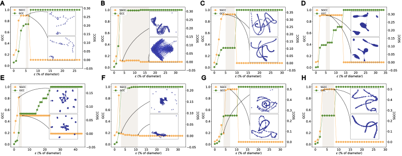
Fig. S10: The phase diagram for constructing networks from 2D benchmark vector data. (A) The test case in Ref.[71], for which the DDB algorithm [16] fails. (B) Flame [78]. (C) Spiral [79]. (D) Aggregation [80].(E) R15 [81]. (F) Blobs with 500 points. (G) Circles with 300 points. (H) Moons with 300 points. (F)-(H) are generated by the standard scikit-learn 0.19.2 in Python (https://pypi.org/project/scikit-learn/0.19.2/). The original spatial layout of vector data is shown in Fig. S11. The largest giant connected component (GCC) represents the ratio of the size of the maximal connected sub-graph to the size of the network, and SGCC represents the second-largest maximal connected graph. The shading area indicates the optimal range of ${\varepsilon}$, during which the LS method can get the correct partition that align with the common consensus. (Insets) Corresponding constructed networks.

In this paper, we use $\varepsilon$-ball method to construct networks from vector data. Its main advantage in our context is its ability to separate local and global information with an appropriate value of $\varepsilon$. Classical clustering methods (e.g., k-means, which are effective on spherical data) are typically unable to group vector data with arbitrary shape (see Fig. S11B-D,G,H), one of the reason is their inability to capture continuity in local information. For example, in Fig. S11H, based on the global metric, every point is accessible to others, and the Euclidean distance between the two end nodes in the red group are farther than to some points in the blue group; when based on the local metric, only points within $\varepsilon$-ball of the point are accessible, and the two end nodes in the red group are reachable to each other but is not reachable to any point in the blue cluster when $\varepsilon$ is not very large.

Building networks via the $\varepsilon$-ball method, which can be accelerated by R-tree data structure [67, 63], with a proper distance threshold $\varepsilon$ can naturally help on separate local metrics from global ones.

However, determining $\varepsilon$ used to be based on empirical experience and usually subject to arbitrariness [71], with similar problems existing in many clustering methods (e.g., DBSCAN [88] or DDB [16]). When building networks using the $\varepsilon$-ball method, the network will undergo a transition from isolated nodes or connected components to a fully connected complete graph as the value of $\varepsilon$ increases. A critical value for $\varepsilon$ can be derived from percolation phase transition as the value for which the size of the second largest connected component is maximal [68, 69, 70].

Experimental results indicate that setting $\varepsilon$ near the critical value when building networks from vector data is usually a good choice to balance local and global structures (see Fig. S10 and corresponding clustering results by the LS algorithm in Fig. S11). In addition, the range of $\varepsilon$ is not narrow in most cases (see Fig. S10), giving a notion of stability to the resulting networks. With a similar idea, some works chose the value of $\varepsilon$ such the network is fully connected [65], but it may not be always the optimal setting. After the critical point of the percolation phase transition, isolated nodes or small-sized groups of nodes can be considered as noisy data that do not belong to any cluster (see grey nodes in Fig. S11B,F). We find that with the presence of non-spherical data (see examples in Fig. S10A,C,G,H), the LS algorithm can have a better performance if $\varepsilon$ is chosen before the critical point; in other cases, a value higher than the critical point (see Fig. S10B,E,F). However, this is just a rough summary from cases in this work, and the reason behind is not the focus of this paper and worth future closer investigations.

Applying the LS algorithm to the network built around the critical threshold value, we can obtain the partition results as shown in Fig. 6 in the main text and Fig. S11 according to the decision graph (see Fig. S12). In contrast, on the same constructed networks from the vector data, the Louvain algorithm cannot obtain partitions that align with the common consensus (see Fig. S13), which tend to have more smaller clusters in a more segmented way.

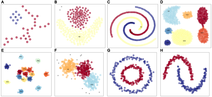
Fig. S11: The original spatial layout of 2D benchmark vector data and clustering results obtained by the LS algorithm on networks constructed from them. (A)-(H) corresponds to clustering results obtained from networks in the optimal range in Fig. S10. Node color indicates clustering partitions. Grey nodes corresponds to identified noisy data. The index of identified cluster centers are labeled in the figure.

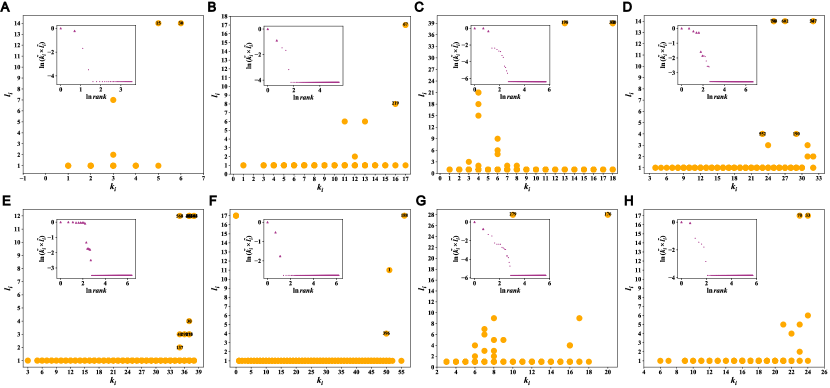
Fig. S12: Identification of cluster centers for 2D benchmark vector data by the LS algorithm. (A)-(H) corresponds to networks in Fig. S10, whose original spatial layout is shown in Fig. S11. (Insets) Decision graphs. Identified cluster centers are highlighted by larger triangles.

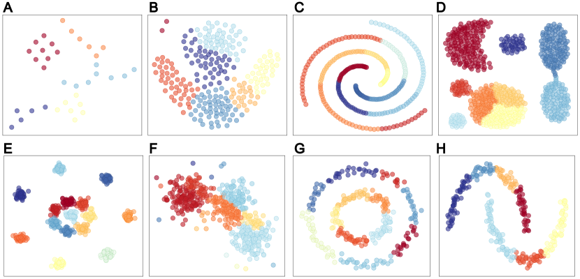
Fig. S13: Clustering results obtained by the Louvain algorithm on networks constructed from vector data. The Louvain algorithm works on the same network constructed from vector data as of the LS method. Node color indicates clustering partitions.

C.1.1 The advantage of building networks for clustering high dimensional vector data

Apart from 2-dimensional benchmark vector data, datasets with very high dimensions are very common in practice. We further apply our LS algorithm to several high dimensional datasets, including Iris [89] (see Fig. S14), Wine [90] (see Fig. S15), MNIST [73] (see Fig. S16), Olivetti [74] (see Fig. S17 and Fig. S18).

• The Iris flower data set is 4-dimensional and contains 50 samples of 3 species (Iris setosa, Iris virginica, and Iris versicolor). Each sample has four features: the length and width of both sepals and petals.

• The Wine data set is of 13-dimension that contains 178 samples of 3 cultivars. The 13 features are the quantities of 13 constituents by the chemical analysis of the 3 cultivars, including alcohol, malic acid, ash, alcalinity of ash, magnesium, total phenols, flavanoids, nonflavanoid phenols, proanthocyanins, color intensity, hue, OD280/OD315 of diluted wines and proline.

• The MNIST handwritten digit dataset is obtained from the National Institute of Standards and Technology, which is widely used in machine learning. It is of 784 (28$\times$28)-dimension and contains 60,000 samples of 10 classes, each of which corresponds to 0-9, respectively. We randomly sample 1,000 figures of 10 digits, and each digit has 100 samples.

• The Olivetti database of human face is widely used in machine learning. It is of 10,304 (92$\times$112)-dimension and contains 400 samples of 10 classes, each of which is consisted of the 40 photos of a person, respectively. The positions of the faces in the photos are the same.

For these high dimensional vector data, the phase transition diagrams and corresponding decision graphs are shown in Figs. S14-S18. The networks we choose to perform the LS algorithm are highlighted by the red dot in Figs. S14-S18, and they are near the critical point of the percolation phase transition. Though degree can be regarded as an analogy to density, and path length as an analogy to Euclidean distance from an object to a nearest larger object, the LS algorithm can have a better performance than the DDB algorithm [16] on datasets with relatively high dimensions. Possible reasons behind the good performance of the LS algorithm might reside in the network construction, which can be regarded as a coarse-graining process and noise filtering, and this also helps on better identifying asymmetric relation between objects.

For the Olivetti dataset, which is a typical example of a challenging high dimensional dataset with small sample size (each person only has ten images, each of which is of 10,304 pixels), we still calculate the Euclidean distance between objects (instead of a more complicated “complex wavelet structural similarity (CW-SSIM)” image similarity measure [91, 16]), and we do not perform a stricter association criterion as in ref.[16]. The LS algorithm clearly identifies 9 and 33 clusters for the Olivetti dataset with 100 images and all 400 images, respectively. In contrast, the DDB algorithm does not identify the correct number of clusters (note that in Table 2 in the main text, we report the result when we manually set the number of clusters as 10 and 40 for DDB, respectively). Besides, we can recognise more images of each individual than the DDB method (see Fig. 4D in ref. [16] and Fig. S19B for comparisons), as reflected by a higher $F_{1}$ score. And each cluster only comprise images of the same object.

In more complex situations with more objects and clusters, the phase diagram also can be more complex with stronger fluctuations. Compared to the Olivetti dataset with the first 100 images, whose phase transition diagram is quite clear (see Fig. S17), when we analyze the Olivetti dataset with all 400 images for 40 persons, its phase diagram become more complex with stronger fluctuations (see Fig. S18), which is also the cases for MNIST dataset (see Fig. S16).

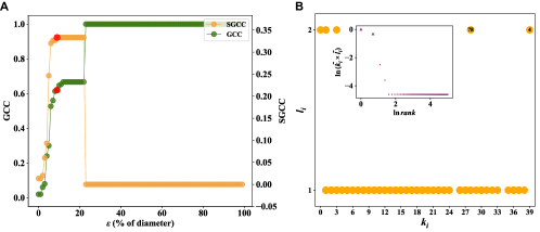
Fig. S14: The phase transition diagram and decision graph for Iris data set. (A) The distribution of GCC and SGCC on Iris data set. (B) The decision graph for Iris data set. ${\varepsilon}$=9% diameter of the original vector data, where the diameter equals the longest distance between any two objects. Three cluster centers are highlighted by larger triangles.

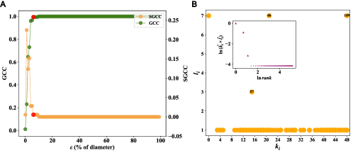
Fig. S15: The phase transition diagram and decision graph for Wine data set. (A) The distribution of GCC and SGCC on Wine data set. (B) The decision graph for Wine data set. ${\varepsilon}$=6% diameter of the original vector data, where the diameter equals the longest distance between any two objects. Two cluster centers are highlighted by larger triangles.

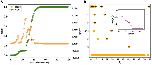
Fig. S16: The phase transition diagram and decision graph for MNIST data set.(A) The phase transition diagram and (B) decision graph for 1000 sampling data from MNIST handwritten digits database. There are 10 classes in total and every class has 100 grayscale image with a size of 28$\times$28 pixels. ${\varepsilon}$=36% diameter of the original vector data, where the diameter equals the longest distance between any two objects. Nine cluster centers are highlighted by larger triangles.

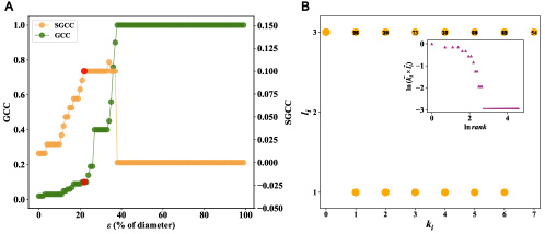
Fig. S17: The phase transition diagram and decision graph for Olivetti sample database. (A) The phase transition diagram and (B) decision graph for the first 100 images of Olivetti database, the number of clusters is 10, with 10 image for each cluster in 92$\times$112 dimensions. ${\varepsilon}$=22% diameter of the original vector data, where the diameter equals the longest distance between any two objects. Nine cluster centers are highlighted by larger triangles.

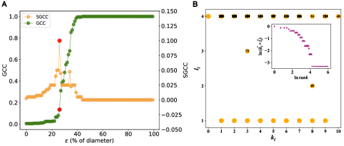
Fig. S18: The phase transition diagram and decision graph for Olivetti database. (A) The phase transition diagram and (B) decision graph for the whole Olivetti database, the number of clusters is 40, with 10 images for each clusters in 92$\times$112 dimensions. ${\varepsilon}$=26% diameter of the original vector data, where the diameter equals the longest distance between any two objects. Thirty-three cluster centers are highlighted by larger triangles.

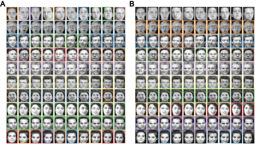
Fig. S19: The clustering result by Louvain and our LS algorithm on the Olivetti data set [84] with its first 100 images.(A) Louvain and (B) Ls algorithm, Each identified category is indicated by the color of rectangle border of the figure, and the black color corresponds to noisy objects identified by our method. See the phase transition diagram and decision graph in Fig. S17. This example further demonstrates the strength of our framework on high-dimensional vector data (see comparisons on $F_{1}$ scores between our LS method and the DDB algorithm [16] in Table 2 in the main text.

Supplementary Text D   Robustness tests of LS algorithm

D.1 Robustness tests on vector data

We first test our LS algorithm on the Clusterable-data dataset (https://www.kaggle.com/lvk110395/clusterable-datanpy) that contains many noisy points (see Fig. S20). The result obtained by the LS algorithm (see Fig. S20) is quite comparable to results by the HDBSCAN method [92]. For the S-sets dataset that comprises 15 Gaussian clusters, with the increase of degree of cluster overlapping (see Fig. S21A-D), the clustering results obtained by our LS algorithm remain relatively robust with the $F_{1}$-score equals 0.99, 0.94, 0.74, 0.62, respectively.

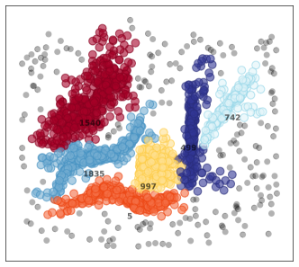
Fig. S20: Clustering result obtained by the LS algorithm on the Clusterable-data dataset. Grey points are identified as noise or can be regarded as cluster halos. Different clusters are indicated by different colors, and the index of cluster centers are labeled.

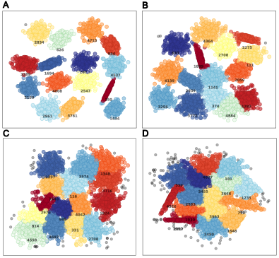
Fig. S21: Clustering results on S-sets dataset by the LS algorithm. S-sets dataset comprises 15 Gaussian clusters with different degree of cluster overlap and standard deviations. Along with the increase of the degree of cluster overlapping from (A)-(D). $F_{1}$ scores are 0.99, 0.94, 0.74, 0.62 for (A)-(D), respectively. Grey points are identified noisy data.

D.2 Robustness tests on networks

In networks, we first test on two common scenarios: randomly removing from or adding edges to the original networks. Our LS algorithm is generally more robust in most networks against random noises in both cases than the Louvain algorithm (see Fig. S22 and Fig. S23). Due to the nature of our method, the LS algorithm is quite vulnerable to targeted failures that connects largest nodes (i.e., we sequentially add edges between the largest node to the remaining forty-nine largest nodes if they were disconnected, see results in Fig. S24). For example, when two local leaders are connected, one will be diminished as a follower, and its community will not be correctly detected. Very occasionally, when the whole network is dominated by a few large communities, adding edges between large nodes make the LS algorithm detect fewer communities and have a higher $F_{1}$-score (see Fig. S24F). Results shown in Figs. S22-S23 are average of ten realizations, and results in Fig. S24 is just one realization, as the network structure is definite.

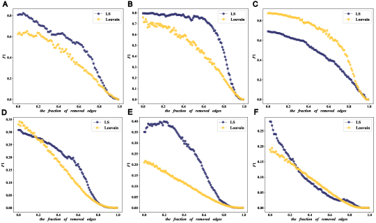
Fig. S22: The comparison between our LS algorithm and Louvian method on $F_{1}$ scores along with randomly removing edges in six networks with ground-truth community labels. (A) Zachary Karate Club [39], (B) Polbooks [82], (C) Polblogs [52], (D) Cora [83], (E) Citeseers [84], and (F) Pubmed [85]. Our LS algorithm is generally more robust against missing links in most networks, which is indicated by higher $F_{1}$-scores and a flatter decreasing.

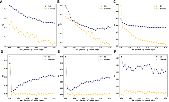
Fig. S23: The comparison between our LS algorithm and Louvian method on $F_{1}$ scores along with randomly adding edges in six networks with ground-truth community labels. (A)-(F) correspond to the same networks in Fig. S22. Our LS algorithm is generally more robust against added noisy links in most networks, which is indicated by higher $F_{1}$-scores.

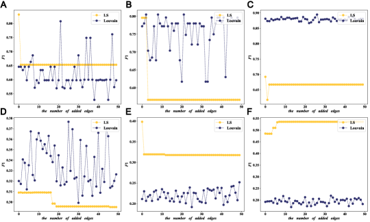
Fig. S24: The targeted failure that adding edges between largest nodes. (A)-(F) correspond to the same networks in Fig. S22. For such targeted failures, it usually diminish one previous community center as a follower, and in this case, the number of communities detected by the LS algorithm will decrease.

References

- [1] Manning, C. D., Raghavan, P. & Schütze, H. Introduction to Information Retrieval (Cambridge University Press, 2008).
- [2] Albert, R. & Barabási, A.-L. Statistical mechanics of complex networks. \JournalTitleReviews of Modern Physics 74, 47 (2002).
- [3] Barabási, A.-L. Network Science (Cambridge University Press, 2016).
- [4] Newman, M. Networks (Oxford University Press, 2018).
- [5] McPherson, M. An ecology of affiliation. \JournalTitleAmerican Sociological Review 519–532 (1983).
- [6] Blondel, V. D., Decuyper, A. & Krings, G. A survey of results on mobile phone datasets analysis. \JournalTitleEPJ Data Science 4, 10 (2015).
- [7] Liu, C. et al. Revealing spatio-temporal interacting patterns behind complex cities. \JournalTitleChaos 32, 081105 (2022).
- [8] Girvan, M. & Newman, M. E. Community structure in social and biological networks. \JournalTitleProceedings of the National Academy of Sciences 99, 7821–7826 (2002).
- [9] Blondel, V. D., Guillaume, J.-L., Lambiotte, R. & Lefebvre, E. Fast unfolding of communities in large networks. \JournalTitleJournal of Statistical Mechanics: Theory and Experiment 2008, P10008 (2008).
- [10] Fortunato, S. Community detection in graphs. \JournalTitlePhysics Reports 486, 75–174 (2010).
- [11] Fortunato, S. & Hric, D. Community detection in networks: A user guide. \JournalTitlePhysics Reports 659, 1–44 (2016).
- [12] Holme, P., Huss, M. & Jeong, H. Subnetwork hierarchies of biochemical pathways. \JournalTitleBioinformatics 19, 532–538 (2003).
- [13] Palla, G., Derényi, I., Farkas, I. & Vicsek, T. Uncovering the overlapping community structure of complex networks in nature and society. \JournalTitleNature 435, 814–818 (2005).
- [14] Clauset, A., Moore, C. & Newman, M. E. Hierarchical structure and the prediction of missing links in networks. \JournalTitleNature 453, 98–101 (2008).
- [15] Kaufman, L. & Rousseeuw, P. J. Finding groups in data: an introduction to cluster analysis (John Wiley & Sons, 2009).
- [16] Rodriguez, A. & Laio, A. Clustering by fast search and find of density peaks. \JournalTitleScience 344, 1492–1496 (2014).
- [17] Li, H.-J. & Daniels, J. J. Social significance of community structure: Statistical view. \JournalTitlePhysical Review E 91, 012801 (2015).
- [18] Blondel, V. D., Guillaume, J.-L., Hendrickx, J. M., de Kerchove, C. & Lambiotte, R. Local leaders in random networks. \JournalTitlePhysical Review E 77, 036114 (2008).
- [19] Serrano, M. Á., Boguná, M. & Vespignani, A. Extracting the multiscale backbone of complex weighted networks. \JournalTitleProceedings of the National Academy of Sciences 106, 6483–6488 (2009).
- [20] Stanoev, A., Smilkov, D. & Kocarev, L. Identifying communities by influence dynamics in social networks. \JournalTitlePhysical Review E 84, 046102 (2011).
- [21] Lee, M. J. et al. Uncovering hidden dependency in weighted networks via information entropy. \JournalTitlePhysical Review Research 3, 043136 (2021).
- [22] Li, R. et al. Gravity model in dockless bike-sharing systems within cities. \JournalTitlePhysical Review E 103, 012312 (2021).
- [23] Newman, M. E. Modularity and community structure in networks. \JournalTitleProceedings of the National Academy of Sciences 103, 8577–8582 (2006).
- [24] Fortunato, S. & Newman, M. E. 20 years of network community detection. \JournalTitleNature Physics 18, 848–850 (2022).
- [25] Clauset, A., Newman, M. E. & Moore, C. Finding community structure in very large networks. \JournalTitlePhysical Review E 70, 066111 (2004).
- [26] Rosvall, M. & Bergstrom, C. T. Maps of random walks on complex networks reveal community structure. \JournalTitleProceedings of the National Academy of Sciences 105, 1118–1123 (2008).
- [27] Peel, L., Larremore, D. B. & Clauset, A. The ground truth about metadata and community detection in networks. \JournalTitleScience Advances 3, e1602548 (2017).
- [28] Duch, J. & Arenas, A. Community detection in complex networks using extremal optimization. \JournalTitlePhysical Review E 72, 027104 (2005).
- [29] McLachlan, G. J. & Krishnan, T. The EM algorithm and extensions, vol. 382 (John Wiley & Sons, 2007).
- [30] Raghavan, U. N., Albert, R. & Kumara, S. Near linear time algorithm to detect community structures in large-scale networks. \JournalTitlePhysical Review E 76, 036106 (2007).
- [31] Frey, B. J. & Dueck, D. Clustering by passing messages between data points. \JournalTitleScience 315, 972–976 (2007).
- [32] Delvenne, J.-C., Yaliraki, S. N. & Barahona, M. Stability of graph communities across time scales. \JournalTitleProceedings of the National Academy of Sciences 107, 12755–12760 (2010).
- [33] Ravasz, E., Somera, A. L., Mongru, D. A., Oltvai, Z. N. & Barabási, A.-L. Hierarchical organization of modularity in metabolic networks. \JournalTitleScience 297, 1551–1555 (2002).
- [34] Sales-Pardo, M., Guimera, R., Moreira, A. A. & Amaral, L. A. N. Extracting the hierarchical organization of complex systems. \JournalTitleProceedings of the National Academy of Sciences 104, 15224–15229 (2007).
- [35] Hoffmann, T., Peel, L., Lambiotte, R. & Jones, N. S. Community detection in networks without observing edges. \JournalTitleScience Advances 6, eaav1478 (2020).
- [36] Reichardt, J. & Bornholdt, S. When are networks truly modular? \JournalTitlePhysica D 224, 20–26 (2006).
- [37] Zitnik, M., Sosič, R. & Leskovec, J. Prioritizing network communities. \JournalTitleNature Communications 9, 2544 (2018).
- [38] Guimera, R. & Nunes Amaral, L. A. Functional cartography of complex metabolic networks. \JournalTitleNature 433, 895–900 (2005).
- [39] Zachary, W. W. An information flow model for conflict and fission in small groups. \JournalTitleJournal of Anthropological Research 33, 452–473 (1977).
- [40] Holland, P. W., Laskey, K. B. & Leinhardt, S. Stochastic blockmodels: First steps. \JournalTitleSocial Networks 5, 109–137 (1983).
- [41] Newman, M. E. & Clauset, A. Structure and inference in annotated networks. \JournalTitleNature Communications 7, 11863 (2016).
- [42] Schaub, M. T. & Peel, L. Hierarchical community structure in networks. \JournalTitlearXiv preprint arXiv:2009.07196 (2020).
- [43] Ravasz, E. & Barabási, A.-L. Hierarchical organization in complex networks. \JournalTitlePhysical Review E 67, 026112 (2003).
- [44] Fortunato, S. & Barthelemy, M. Resolution limit in community detection. \JournalTitleProceedings of the National Academy of Sciences 104, 36–41 (2007).
- [45] Barabási, A.-L. & Albert, R. Emergence of scaling in random networks. \JournalTitleScience 286, 509–512 (1999).
- [46] Mucha, P. J., Richardson, T., Macon, K., Porter, M. A. & Onnela, J.-P. Community structure in time-dependent, multiscale, and multiplex networks. \JournalTitleScience 328, 876–878 (2010).
- [47] Evans, T. S. & Chen, B. Linking the network centrality measures closeness and degree. \JournalTitleCommunications Physics 5 (2022).
- [48] Yang, J. & Leskovec, J. Defining and evaluating network communities based on ground-truth. \JournalTitleKnowledge and Information Systems 42, 181–213 (2015).
- [49] Evans, T. S. Clique graphs and overlapping communities. \JournalTitleJournal of Statistical Mechanics: Theory and Experiment P12037 (2010).
- [50] Evans, T. S. American college football network files, DOI: 10.6084/M9.FIGSHARE.93179.V2.
- [51] Palla, G., Barabási, A.-L. & Vicsek, T. Quantifying social group evolution. \JournalTitleNature 446, 664–667 (2007).
- [52] Adamic, L. A. & Glance, N. The political blogosphere and the 2004 us election: divided they blog. In Proceedings of the 3rd International Workshop on Link Discovery, 36–43 (2005).
- [53] Hric, D., Darst, R. K. & Fortunato, S. Community detection in networks: structural clusters versus ground truth. \JournalTitlePhysical Review E 90, 062805 (2014).
- [54] Louf, R. & Barthelemy, M. Modeling the polycentric transition of cities. \JournalTitlePhysical Review Letters 111, 198702 (2013).
- [55] Alexander, L., Jiang, S., Murga, M. & González, M. C. Origin–destination trips by purpose and time of day inferred from mobile phone data. \JournalTitleTransportation Research Part C: Emerging Technologies 58, 240–250 (2015).
- [56] Çolak, S., Alexander, L. P., Alvim, B. G., Mehndiratta, S. R. & González, M. C. Analyzing cell phone location data for urban travel: current methods, limitations, and opportunities. \JournalTitleTransportation Research Record 2526, 126–135 (2015).
- [57] Çolak, S., Lima, A. & González, M. C. Understanding congested travel in urban areas. \JournalTitleNature Communications 7, 10793 (2016).
- [58] Dong, L., Li, R., Zhang, J. & Di, Z. Population-weighted efficiency in transportation networks. \JournalTitleScientific Reports 6, 26377 (2016).
- [59] Li, R., Wang, W. & Di, Z. Effects of human dynamics on epidemic spreading in Côte d’Ivoire. \JournalTitlePhysica A 467, 30–40 (2017).
- [60] Xu, Y., Li, R., Jiang, S., Zhang, J. & González, M. C. Clearer skies in Beijing — revealing the impacts of traffic on the modeling of air quality. In The 96th Annual Meeting of Transportation Research Board, Washington DC, 17-05211 (2017).
- [61] Xu, Y. et al. Unraveling environmental justice in ambient pm2.5 exposure in Beijing: A big data approach. \JournalTitleComputers, Environment and Urban Systems 75, 12–21 (2019).
- [62] Schläpfer, M. et al. The scaling of human interactions with city size. \JournalTitleJournal of the Royal Society Interface 11, 20130789 (2014).
- [63] Li, R. et al. Simple spatial scaling rules behind complex cities. \JournalTitleNature Communications 8, 1841 (2017).
- [64] Qian, Y., Expert, P., Panzarasa, P. & Barahona, M. Geometric graphs from data to aid classification tasks with graph convolutional networks. \JournalTitlePatterns 2, 100237 (2021).
- [65] Bullmore, E. T. & Bassett, D. S. Brain graphs: graphical models of the human brain connectome. \JournalTitleAnnual Review of Clinical Psychology 7, 113–140 (2011).
- [66] Berenhaut, K. S., Moore, K. E. & Melvin, R. L. A social perspective on perceived distances reveals deep community structure. \JournalTitleProceedings of the National Academy of Sciences 119 (2022).
- [67] Guttman, A. R-trees: A dynamic index structure for spatial searching. In Proceedings of the 1984 ACM SIGMOD International Conference on Management of Data, 47–57 (1984).
- [68] Bollobás, B. & Béla, B. Random graphs. 73 (Cambridge University Press, 2001).
- [69] Bunde, A. & Havlin, S. Fractals and disordered systems (Springer Science & Business Media, 2012).
- [70] Li, D. et al. Percolation transition in dynamical traffic network with evolving critical bottlenecks. \JournalTitleProceedings of the National Academy of Sciences 112, 669–672 (2015).
- [71] Pizzagalli, D. U., Gonzalez, S. F. & Krause, R. A trainable clustering algorithm based on shortest paths from density peaks. \JournalTitleScience Advances 5, eaax3770 (2019).
- [72] Traag, V. A., Waltman, L. & Van Eck, N. J. From Louvain to Leiden: guaranteeing well-connected communities. \JournalTitleScientific Reports 9, 5233 (2019).
- [73] Chatfield, K., Lempitsky, V. S., Vedaldi, A. & Zisserman, A. The devil is in the details: an evaluation of recent feature encoding methods. In Proceedings of the British Machine Vision Conference, 76.1–76.12 (2011).
- [74] Samaria, F. S. & Harter, A. C. Parameterisation of a stochastic model for human face identification. In Proceedings of 1994 IEEE Workshop on Applications of Computer Vision, 138–142 (IEEE, 1994).
- [75] Evans, T. S. & Lambiotte, R. Line graphs, link partitions and overlapping communities. \JournalTitlePhys.Rev.E 80, 016105 (2009).
- [76] Evans, T. S. & Lambiotte, R. Line graphs of weighted networks for overlapping communities. \JournalTitleEuropean Physical Journal B 77, 265–272 (2010).
- [77] Ahn, Y.-Y., Bagrow, J. P. & Lehmann, S. Link communities reveal multiscale complexity in networks. \JournalTitleNature 466, 761–764 (2010).
- [78] Fu, L. & Medico, E. Flame, a novel fuzzy clustering method for the analysis of dna microarray data. \JournalTitleBMC Bioinformatics 8, 1–15 (2007).
- [79] Chang, H. & Yeung, D.-Y. Robust path-based spectral clustering. \JournalTitlePattern Recognition 41, 191–203 (2008).
- [80] Gionis, A., Mannila, H. & Tsaparas, P. Clustering aggregation. \JournalTitleAcm transactions on knowledge discovery from data (tkdd) 1, 4–es (2007).
- [81] Veenman, C. J., Reinders, M. J. T. & Backer, E. A maximum variance cluster algorithm. \JournalTitleIEEE Transactions on pattern analysis and machine intelligence 24, 1273–1280 (2002).
- [82] Krebs, V. Social network analysis software & services for organizations, communities, and their consultants (2013).
- [83] Rossi, R. & Ahmed, N. The network data repository with interactive graph analytics and visualization. In Twenty-Ninth AAAI Conference on Artificial Intelligence (2015).
- [84] Bollacker, K. D., Lawrence, S. & Giles, C. L. Citeseer: An autonomous web agent for automatic retrieval and identification of interesting publications. In Proceedings of the second international conference on Autonomous agents, 116–123 (1998).
- [85] Sen, P. et al. Collective classification in network data. \JournalTitleAI magazine 29, 93–93 (2008).
- [86] Pons, P. & Latapy, M. Computing communities in large networks using random walks. In International symposium on computer and information sciences, 284–293 (Springer, 2005).
- [87] Reichardt, J. & Bornholdt, S. Statistical mechanics of community detection. \JournalTitlePhysical review E 74, 016110 (2006).
- [88] Ester, M., Kriegel, H.-P., Sander, J., Xu, X. et al. A density-based algorithm for discovering clusters in large spatial databases with noise. In KDD, vol. 96, 226–231 (1996).
- [89] Fisher, R. The use of multiple measures in taxonomic problems. \JournalTitleAnn. Eugenics 7, 179–188 (1936).
- [90] Aeberhard, S., Coomans, D. & De Vel, O. Comparative analysis of statistical pattern recognition methods in high dimensional settings. \JournalTitlePattern Recognition 27, 1065–1077 (1994).
- [91] Sampat, M. P., Wang, Z., Gupta, S., Bovik, A. C. & Markey, M. K. Complex wavelet structural similarity: A new image similarity index. \JournalTitleIEEE transactions on image processing 18, 2385–2401 (2009).
- [92] Campello, R. J., Moulavi, D. & Sander, J. Density-based clustering based on hierarchical density estimates. In Pacific-Asia conference on knowledge discovery and data mining, 160–172 (Springer, 2013).