Augmentation Invariant Discrete Representation for
Generative Spoken Language Modeling

Abstract

Generative Spoken Language Modeling research focuses on optimizing speech Language Models (LMs) using raw audio recordings without accessing any textual supervision. Such speech LMs usually operate over discrete units obtained from quantizing internal representations of self-supervised models. Although such units show impressive modeling results, their robustness capabilities have not been extensively investigated. This work focuses on improving the robustness of discrete input representations for generative spoken language modeling. First, we formally define how to measure the robustness of such representations to various signal variations that do not alter the spoken information (e.g., time-stretch). Next, we empirically demonstrate how current state-of-the-art representation models lack robustness to such variations. To overcome this, we propose an effective and efficient method to learn robust discrete speech representation for generative spoken language modeling. The proposed approach is based on applying a set of signal transformations to the speech signal and optimizing the model using an iterative pseudo-labeling scheme. Our method significantly improves over the evaluated baselines when considering encoding and modeling metrics. We additionally evaluate our method on the speech-to-speech translation task, considering Spanish-English and French-English translations, and show the proposed approach outperforms the evaluated baselines.

1 Introduction

Self-supervised speech models were shown to learn effective representations for various downstream tasks (Hsu et al., 2021; Chen et al., 2022; Baevski et al., 2020). These models were mainly evaluated on discriminative tasks, such as automatic speech recognition, speaker verification, intent classification, etc. (Yang et al., 2021). Recently, Lakhotia et al. (2021) demonstrated that such self-supervised learning (SSL) representations can be used for Generative Spoken Language Modeling.

Generative Spoken Language Modeling (GSLM) is the task of learning the acoustic and linguistic characteristics of a language from raw audio. In other words, a discrete representation of the audio signal is being learned. A common practice is to extract continuous representation using an SSL model, then apply vector quantization, usually using the k-means algorithm (Lakhotia et al., 2021; Kharitonov et al., 2021a; Borsos et al., 2022). Then a speech-language model is trained on top of the obtained representation. Finally, a neural vocoder converts the output units to raw audio. As the discrete speech representation often operates over units extracted over relatively short windows (e.g., 20ms), sequences can be long and contain repetitions, e.g., 10 11 11 11 21 32 32 32 21. Preliminary studies have found that removing sequential repetitions of units improves performance, hence applying it universally (Lakhotia et al., 2021). For example, a pseudo-text 10 11 11 11 21 32 32 32 21 becomes 10 11 21 32 21. This framework was shown to be effective in modeling multiple levels of the speech utterance, namely prosody, and content (Lakhotia et al., 2021; Kharitonov et al., 2021a; Borsos et al., 2022), speech codec (Polyak et al., 2021), speech emotion conversion (Kreuk et al., 2021), spoken dialogue (Nguyen et al., 2022), and speech-to-speech translation (Lee et al., 2021; Popuri et al., 2022; Lee et al., 2022).

An essential prerequisite for such an audio representation to be used in real-world conditions is robustness to various signal corruptions. Although the aforementioned audio representation models have shown effectiveness in many tasks, they were mainly evaluated on academic benchmarks.

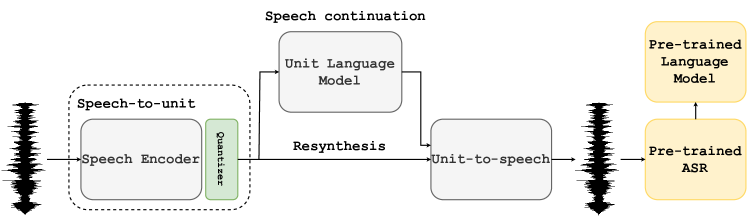
Figure 1: Generative Spoken Language Modeling is composed of three components: (i) Speech-to-unit, (ii) Unit language model, and (iii) Unit-to-speech. Pre-trained ASR and language models are used for evaluation.

In this work, we evaluate current state-of-the-art self-supervised speech representation models on what are arguably the most basic signal variations, namely time-stretch, pitch-shift, additive-noise, and reverberation. Our premise is that while these variations modify the signal, its’ underlying content remains the same, especially under the units repetition removal process. Therefore, a robust representation should be affected by such variations to a minimal extent.

As a first step, we propose a set of metrics for evaluating the model’s robustness. Then, we point to the lack of robustness of these models with respect to the aforementioned variations. Next, we design a simple and effective method for learning robust discrete representation on top of any speech SSL model. We demonstrate how such a method greatly improves robustness. Then, we empirically show that performance improves on several tasks for various SSL models. Specifically, we evaluate the newly proposed speech encoders when considering zero-shot evaluation tasks considering encoding and modeling, i.e., ABX, sWUGGY, and sBLIMP (Nguyen et al., 2020), together with a high-level downstream task in the form of speech-to-speech translation.

2 Background

The general Generative Spoken Language Modeling (GSLM) pipeline is comprised of three main modules: (i) Speech-to-unit, (ii) Unit language model, and (iii) Unit-to-speech, where each of these modules is trained separately. Speech resynthesis can be achieved while ignoring the language model and directly feeding the quantized units into the unit-to-speech module (Polyak et al., 2021) (See Figure 1 for a visual description). In the following paragraphs, we give detailed background for each of the three components mentioned above, including the standard evaluation methods.

Speech-to-unit

module encodes the raw speech signal into a discrete representation. The common approach is first to encode the speech into a continuous representation and then quantize the representation to achieve a sequence of discrete units (Lakhotia et al., 2021; Polyak et al., 2021; Popuri et al., 2022; Lee et al., 2021; Kharitonov et al., 2021a; Kreuk et al., 2021; Kharitonov et al., 2022; Nguyen et al., 2022; Borsos et al., 2022; Tjandra et al., 2019, 2020).

Formally, denote the domain of audio samples by $\mathcal{X}\subset\mathbb{R}$. The representation for a raw signal is therefore a sequence of samples $x=(x_{1},\ldots,x_{T})$, where $x_{t}\in\mathcal{X}$ for all $1\leq t\leq T$.

Consider an encoder network, $f$, that gets as input the speech utterance and outputs a sequence of spectral representations sampled at a low frequency as follows $f(x)=(v_{1},\dots,v_{T^{\prime}})$. Note that we do not assume anything about the structure of the encoder network $f$. Lakhotia et al. (2021), evaluated several speech encoders, namely, Mel-spectrogram, Contrastive Predictive Coding (Oord et al., 2018, CPC), wav2vec2 (Baevski et al., 2020), and HuBERT (Hsu et al., 2021).

Since the representations learned by such models are usually continuous, a k-means algorithm is applied over the models’ outputs to generate discrete units, denoted as $z=(z_{1},\ldots,z_{T^{\prime}})$. Each element $z_{i}$ in $z$ is a positive integer, $z_{i}\in\{1,..,K\}$ for $1\leq i\leq T^{\prime}$, where $K$ is the number of discrete units. We denote the quantization model with $E$.

Unit Language Model

is trained on the extracted discrete units, $z$. Such a language model learns a probability distribution of the learned unit sequences, which enables direct modeling of speech data without textual supervision.

The language model can be used to generate speech conditionally or unconditionally, replicating what toddlers achieve before learning to read. Moreover, such a modeling framework allows for capturing and modeling prosodic features (Kharitonov et al., 2021a), as well as speaker identity (Borsos et al., 2022), or even natural dialogues (Nguyen et al., 2022). This is in contrast to using textual features, as they do not encode such information.

Unit-to-speech

module converts the speech discrete units to a raw waveform. Lakhotia et al. (2021) used a Tacotron2.0 (Shen et al., 2018) based model followed by WaveGlow (Prenger et al., 2019) vocoder. Later, Polyak et al. (2021) proposed a unit-based vocoder based on the HiFi-GAN architecture to convert units to speech directly. Such a paradigm seems to provide high-quality generations with better efficiency as it uses only one model rather than two. Kreuk et al. (2021) and Lee et al. (2021) additionally improved the unit based vocoder to include emotional tokens for speech emotion conversion tasks, and duration modeling for direct speech-to-speech translation.

Zero-shot Evaluation.

Evaluating such a complex pipeline comprised of several components is a challenging task. Lakhotia et al. (2021) proposed a set of zero-shot evaluation tasks aiming for each of the modules. Overall the proposed tasks can be divided into four main groups: (i) acoustic encoding using ABX, bitrat, (ii) language encoding using sWUGGY, sBLIMP (Nguyen et al., 2020; Lakhotia et al., 2021), (iii) resynthesis using Phoneme/Word Error Rate; (iv) speech generation using VERT (Lakhotia et al., 2021), Meaningfulness Mean Opinion Score.

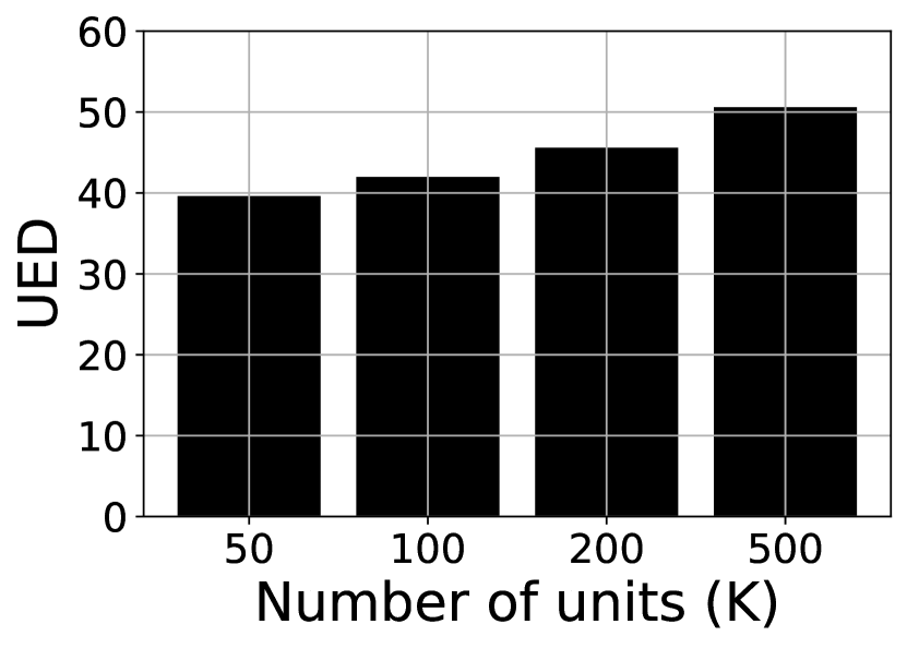
(a) Time stretch

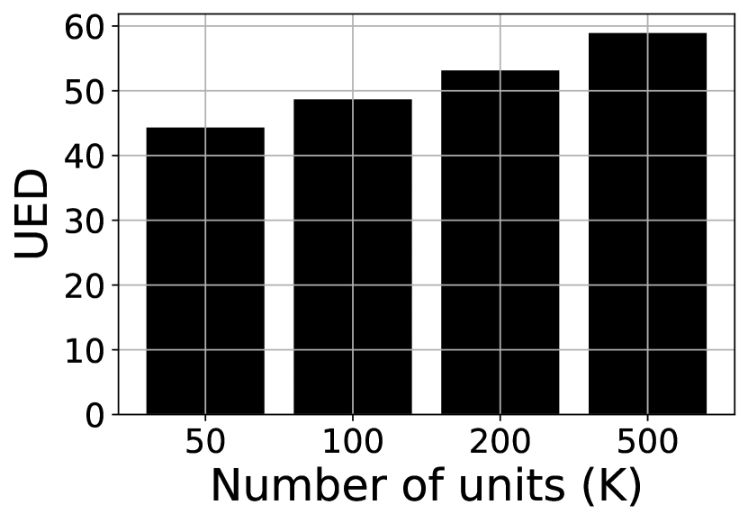
(b) Pitch shift

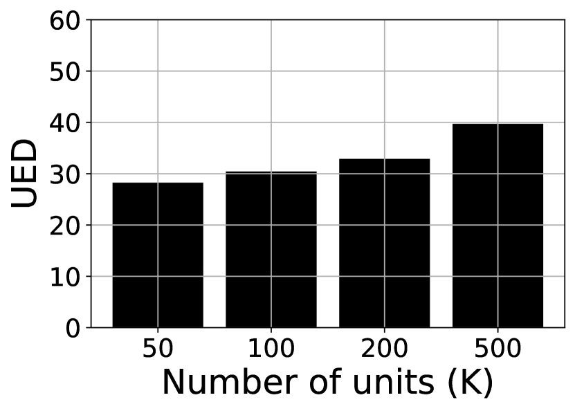
(c) Reverberation

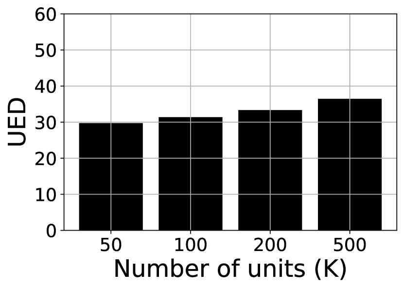
(d) Noise

Figure 2: UED scores for various augmentations and number of clusters. We note that the UED is relatively high (the distance is normalized). We also note that the UED monotonically increases with the number of units used. We multiply the scores by a hundred.

3 Robustness of Speech-to-Unit Models

The first step toward developing an effective spoken language model is to develop a robust representation. The focus of a robust representation should be on the spoken information rather than unrelated signals, such as prosodic features in the form on duration and F0, background noise, or reverberations. In the following section, we propose a metric for quantifying the degree to which augmentations change the resulting encoding.

3.1 Unit Edit Distance

A spoken language model is built on top of a discrete representation of a continuous encoder. We examine the robustness of the discrete space to augmentations that do not change the spoken content. Therefore, we are interested in a sequential distance metric between two discrete representations. It is essential to note that augmentations can alter the spatial dimension of the signal. For example, stretching a signal results in more frames, yielding a longer representation sequence. Similar phenomenon will happen when convolving with different room impulse response to simulate reverberation. Hence, the metric should be able to measure the distance between two sequences of different lengths. Ideally, it will consider the number of deletions, insertions, and substitutions that occur due to augmenting the input data. For this purpose, we find the Levenshtein distance a good fit (Levenshtein, 1966). The Levenshtein distance measures the minimum changes one should make to modify one sequence to another. It has two essential properties: the first is that the score is non-negative, and when the sequences are equal, the metric equals zero. The second property is that the maximum value it can get equals the longer sequence length between the two sequences. We provide a detailed explanation of the Levenshtein distance in the Appendix material.

We aggregate the distance values over the evaluation set while considering the sequence length. This is desirable since we want to normalize scores for sequences in different lengths, and the Levenshtein distance’s maximum value is the original sequence’s length. Another essential property of a spatial metric is repetitions. Consider time stretch as an example, it changes the number of the input frames, but one would expect the deduplicated quantized signal to be the same as before the augmentation. Hypothetically, one can maximize the score by stretching the signal infinitely. To eliminate such dependencies, we compute the score on a deduplicated quantized representation. Formally, our final metric is:

Definition 3.1 (Unit Edit Distance).

Given a continuous encoder $f:\operatorname{\mathbb{R}}^{T}\rightarrow\operatorname{\mathbb{R}}^{T^{\prime}}$, a quantizer $E:\operatorname{\mathbb{R}}^{T^{\prime}}\rightarrow\{1,..,K\}^{T^{\prime}}$, and an input augmentation $g:\operatorname{\mathbb{R}}^{T^{\prime}}\rightarrow\operatorname{\mathbb{R}}^{\widehat{T^{\prime}}}$. The deduplicated unit edit distance $\text{UED}_{\mathcal{D}}(E,f,g)$ on the evaluation set $\mathcal{D}$ is:

$$\sum_{x\in\mathcal{D}}\frac{1}{T^{\prime}_{x}}\text{LEV}\left((E\circ f)(x),(E\circ f\circ g)(x)\right),$$ (1)

where $T^{\prime}_{x}$ is the number of frames of a sample $x$.

Ideally, a perfect spoken language quantizer obtains a zero distance after deduplication. Next, we study state-of-the-art spoken language representations using our proposed metric in different settings.

3.2 Evaluation

In the following, we study current state-of-the-art representations for generative spoken language modeling using the proposed metric. The current popular quantization technique is a k-means model trained on top of a pre-trained encoder (Lakhotia et al., 2021). In our evaluation setup, we use a different number of clusters and encoder architectures. Our ablation study include quantizers with $50$, $100$, $200$, and $500$ clusters. We further investigate our metric on top of HuBERT (Hsu et al., 2021), wav2vec2 (Baevski et al., 2020), and WavLM (Chen et al., 2022). For readability, throughout the paper, we report results for the HuBERT model while leaving the rest of the results in the Appendix material.

3.2.1 Augmentations

This work focus on four simple signal modifications which mimic real-world signal variations:

Time stretch.

We use the Phase Vocoder method (Karrer et al., 2006) to stretch or shrink the time domain signal with a rate of $\tau$ without changing the pitch. For example, $\tau=1.2$ speeds up the signal by $20\%$. In this work, for each sample, we sample uniformly a value in the range $[0.8,1.2]$.

Pitch shift.

We change the original pitch of the speech signal by a given number of semitones using the resampling method over the time-stretched signal (Karrer et al., 2006). In this paper, we shift the pitch by up to four semitones.

Reverberation.

We follow a similar setting of Chazan et al. (2021), in which we consider an Acoustic Transfer Function (ATF) to be simulated using the pyroomacoustics (Scheibler et al., 2018) audio room simulations package. We randomly sample room dimensions, microphone location, and source location, then convolve the ATF with the speech signal.

Noise injection.

We mix a given speech signal with non-stationary additive noise, using a randomly sampled Signal-to-Noise Ratio (SNR) in the range of $[5,15]$. Background noises are sampled from the Deep Noise Suppression (DNS) challenge (Reddy et al., 2020) which includes a diverse set of noise types from AudioSet (Gemmeke et al., 2017), Freesound,  and Demand (Thiemann et al., 2013).

3.2.2 Results

In Figure 2, we use our metric to study the robustness of k-means trained on top of HuBERT with various augmentations and values of $K$. This evaluation points to the lack of robustness of the current state-of-the-art representation of simple, non-spoken augmentations. For example, for time stretch augmentation, the UED score is between $39$ and $51$. Considering that UED is computed on deduplicated signals, those numbers are high. Moreover, this number increases as a function of $K$. The high numbers and the monotonicity of the UED as a function of $K$ are consistent for all values of $K$, augmentations, and models we experimented with (HuBERT, wav2vec2, and WavLM). Next, we propose a method that improves the robustness of such representations.

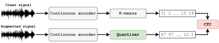
Figure 3: Illustration of our method: We forward a clean signal through an encoder followed by a pre-trained quantizer (k-means). Next, we forward an augmented signal through the same encoder, followed by a new quantizer (green). The CTC loss between the deduplicated output of the clean signal and the output of the augmented signal is used to learn the parameters of the new quantizer. In the iterative approach, post the convergence of the learned quantizer $E_{0}$, we freeze it and learn a new quantizer $E_{1}$ that distills information from $E_{0}$.

4 Pseudo-labeling for Robust Discrete Representation

Our findings in Section 3 suggest that current state-of-the-art representations may be too sensitive to augmentations that do not alter spoken information. Preliminary robustness research focused primarily on noise augmentation. This is convenient since the signal length is not affected by such augmentations. In practice, real-world augmentations may modify the signal length. In order to work with various types of augmentations, we must align the original and augmented sequences. The following section presents a pseudo-labeling, alignment-based approach to learning a robust quantizer.

4.1 Pseudo-labeling

The GSLM encoding framework comprises a raw audio signal forwarded through an encoder, then a quantizer. The quantizer is learned on top of a trained encoder, e.g., k-means trained on each embedding vector extracted from HuBERT.

As discussed above, we do not want to limit the robustness process to a family of augmentations that do not change the signal’s length. To align and use augmentations that may modify the signal’s length, we use the Connectionist Temporal Classification (CTC) loss (Graves et al., 2006). The CTC operation computes the probability of an alignment based on the predicted and target sequences. Finally, the CTC loss considers the negative log-likelihood produced by the CTC operation.

We forward a clean signal through an encoder $f$ followed by a pre-trained quantizer $E_{0}$. Parallelly, we forward an augmented signal through the same encoder $f$ and train a non-linear multi-layer-perceptron $E_{1}$. Using the CTC loss, which accounts for the alignment between the outputs, we learn the parameters of $E_{1}$. Formally, the probability given by the CTC loss $\ell(E_{0},E_{1},x,g)$ for a single data point $x$ follows

$$-p\left((E_{0}\circ f)(x)|(E_{1}\circ f\circ g)(x)\right),$$ (2)

which can be decomposed to a sum over the set of all alignments $\mathcal{A}_{x}$

$$-\sum_{\mathcal{A}\in\mathcal{A}_{x}}\prod_{t=1}^{r}p_{t}(a_{t}|(E_{1}\circ f\circ g)(x)).$$ (3)

Finally, for a training set $\mathcal{D}$, a set of augmentations $\mathcal{G}$, a pre-trained quantizer $E_{0}$, and a learned quantizer $E_{1}$, our loss function is as follows:

$$\mathcal{L}_{\mathcal{D}}(E_{0},E_{1},\mathcal{G})\triangleq\operatorname{\mathbb{E}}_{x\sim\mathcal{D},g\sim\mathcal{U}(\mathcal{G})}\left[\ell(E_{0},E_{1},x,g)\right].$$

Note that the alignment between the predicted and target sequences is many-to-one. Thus, one or more output units can be aligned to a single target unit. Hence, to work with augmentations that stretch the signal, we are required to deduplicate the target sequence. Intuitively, this process distills quantization knowledge from the pre-trained quantizer into the new quantizer while injecting $E_{1}$ knowledge about the contextual similarity between the original and augmented signals.

A significant advantage of our method is that it is highly efficient. Our method requires training only a relatively small amount of parameters. In contrast to previous methods that train HuBERT from scratch, which takes up to seven days on $32$ GPUs, our method converges in a few hours on a single GPU. In fact, our experiments show that learning the parameters of the encoder performs worse than freezing them. While the UED is boosted, but the ABX are negatively affected. The freezing of the upstream model thus serves as a regularizer.

# units	Method	Augmentation
		Time	Pitch shift	Reverberation	Noise
50	k-means	39.61$\pm$0.37	44.33$\pm$0.92	28.25$\pm$0.61	29.74 $\pm$0.31
	Ours	27.91$\pm$0.42	30.74$\pm$0.71	20.16$\pm$0.60	25.33$\pm$0.36
	Ours (Iterative)	26.89$\pm$0.33	30.22$\pm$0.79	19.89$\pm$0.54	24.67$\pm$0.29
100	k-means	41.97$\pm$0.42	48.68$\pm$0.96	30.42$\pm$0.69	31.38$\pm$0.33
	Ours	31.05$\pm$0.39	34.77$\pm$0.92	22.21$\pm$0.63	28.05$\pm$0.31
	Ours (Iterative)	29.72$\pm$0.41	32.84$\pm$0.91	21.31$\pm$0.71	25.06$\pm$0.31
200	k-means	45.59$\pm$0.39	53.14$\pm$1.01	32.89$\pm$0.72	33.34 $\pm$0.38
	Ours	34.40$\pm$0.46	38.51$\pm$1.09	24.10$\pm$0.66	30.19$\pm$0.37
	Ours (Iterative)	32.99$\pm$0.42	36.45$\pm$1.03	22.94$\pm$0.67	26.76 $\pm$0.31
500	k-means	50.60$\pm$0.42	58.92$\pm$0.98	39.71$\pm$0.81	36.47$\pm$0.44
	Ours	38.04$\pm$0.44	43.48$\pm$1.03	28.43$\pm$0.73	29.99$\pm$0.45
	Ours (Iterative)	36.50$\pm$0.49	40.82$\pm$1.02	25.78$\pm$0.74	27.51$\pm$0.49

Table 1: Unit edit distance study: Using our metric, we assess the robustness of various quantization methods on top of a HuBERT representation. This study uses four different augmentations: time stretching, pitch shifting, reverberation, and noise injection. The non-iterative (Section 4.1) and iterative (Section 4.2) methods significantly and consistently improve the robustness of k-means. Pseudo-labeling accounts for most of the improvement. By applying our method iteratively, we can improve it further. For readability, we multiply the scores by a hundred.

4.2 Iterative Pseudo-labeling

In the previous section, we presented a pseudo-labeling approach that relies on a converged quantizer $E_{0}$, e.g., k-means on top of HuBERT. This raises the question of whether it is possible to enhance the robustness of the learned quantizer $E_{1}$ by iteratively replacing the pre-trained quantizer with the converged quantizer and learning another MLP on top of it. It turns out that such a process can further improve the robustness.

The iterative process begins with a pre-trained quantizer $E_{0}$, then, as in Section 4.1 we learn a robust quantizer $E_{1}$. Upon $E_{1}$ convergence, we replace $E_{0}$ with $E_{1}$ and use it as the pre-trained quantizer. Then, we learn a new MLP $E_{2}$ on top of the converged $E_{1}$. We repeat this process $K$ times. This process needs more careful training. We note that it is essential to replace the quantizers only post-convergence.

5 Experiments

In the following, we assess the efficacy of our method using state-of-the-art self-supervised representations and popular discriminative and generative evaluation tasks. It is important to note that a single metric cannot tell the whole story. For example, similarly to perplexity, all representations can be assigned to the same cluster, which achieves a perfect unit edit distance but a poor representation. We first examine our proposed method using the unit edit distance along with other discriminative and generative performance metrics. Then, we show that our method improves downstream tasks.

In Section 5.1 we use our proposed metric from Section 3 to analyze the robustness of our method. In Section 5.2 we study the discriminative capabilities of our method using the ABX test (Schatz et al., 2013). Then, we evaluate our methods using generative zero-shot evaluation tasks such as sWUGGY and sBLIMP (Nguyen et al., 2020; Lakhotia et al., 2021). Finally, we demonstrate the effect of using our robust quantizer’s units in speech-to-speech translation.

Experimental Setup.

We study our method using the base versions of HuBERT, wav2vec2, and WavLM. For readability, we report results for HuBERT in the main paper. The results for wav2vec2 and WavLM are in Appendix C. To match the current k-means training set, we use the Librispeech-100h to learn our quantizer (Panayotov et al., 2015). We analyze our metric using the ‘clean’ and ‘other’ development sets from Librispeech. A detailed setup is provided in Appendix B.

# units	Method	ABX (clean) $\downarrow$		ABX (other)$\downarrow$		sWUGGY $\uparrow$	sBLIMP $\uparrow$
		Within	Across	Within	Across
50	k-means	7.52	8.90	9.84	13.5	66.12	54.91
	Ours	6.76	7.72	9.03	11.78	67.59	55.76
	Ours (Iterative)	6.63	7.55	9.53	12.14	67.42	57.04
100	k-means	6.37	7.72	8.4	12.29	67.70	56.16
	Ours	5.50	6.21	7.24	10.11	67.79	57.01
	Ours (Iterative)	5.39	6.22	7.46	10.20	68.20	56.99
200	k-means	5.99	7.14	8.23	11.51	66.51	54.64
	Ours	5.29	6.01	7.22	9.78	70.51	56.19
	Ours (Iterative)	5.19	6.00	7.18	9.70	70.68	56.26
500	k-means	5.98	6.98	7.89	11.43	66.92	55.97
	Ours	5.16	6.03	7.06	9.76	70.13	55.19
	Ours (Iterative)	4.96	5.73	6.93	9.63	69.33	56.93

Table 2: Zero-shot discriminative and generative evaluation tasks: We evaluate the ABX score on the ‘clean’ and ‘other’ development sets from Librispeech. Our method improves the scores scores in all setups.

5.1 Analysis

In Section 3, we presented an evaluation metric that assesses the robustness of a quantized speech representation to augmentations. The metric is insensitive to changes in the length of the signal. Using it, we investigated the current state-of-the-art representations. In the following, we study our robust quantization method.

Table 1 presents the unit edit distance metric using our robustness method with and without the iterative approach. Compared with the k-means method, which is currently in use, our non-iterative method consistently outperforms it by a large margin (relative improvement of at least 30%). We also note that different augmentations affect the representation differently. Our iterative method provides a slight but consistent improvement over the non-iterative method. It is noticeable that the UED is increasing (i.e., worse performing) with the number of units used.

5.2 Zero-shot Evaluation

We evaluate the proposed method using the standard GSLM setup, i.e., ABX, sWUGGY, sBLIMP. The ABX task examines the discriminative phonetic abilities of the representation.  Versteegh et al. (2015) show that the ABX result is a good proxy to signal content (i.e., Phoneme Error Rate). The input to the ABX is a pair of words with a phoneme modification and a reference word containing the same phoneme as one of the pair’s words. Next, the ABX measures the distance of the test phoneme representation to both the correct and incorrect representations. Finally, the distance between the test and the correct representation is expected to be lower than the distance to the incorrect representation. The ABX task is conducted in two setups: ‘within’ and ‘across.’ ‘Within’ is evaluated on input data from the same speaker, while ‘across’ is evaluated on input data from different speakers.

Table 2 shows the ABX results for both Librispeech ‘clean’ and ‘other’. In our experiments, we found that the ABX score consistently and significantly improved on all the setups we tested. In this case, the iterative approach improves more than the non-iterative one, but the improvement is inconsistent. For a small number of units and the ‘other’ split, the ABX score is lower than the iterative model’s score. Note that the ‘other’ split is challenging as it is characterized by recordings that contain background noise and various accents.

The spot-the-word task (sWUGGY) requires detecting the real word from a pair of short utterances such as ‘brick’ vs. ‘blick.’ The detection is done by comparing the probabilities given by a language model for each word. This allows comparing representations by training language models on top of them. Differently, the acceptability judgment test (sBLIMP) requires detecting the syntactically correct sentence from a pair of sentences, one of which is syntactically correct and the other is wrong. The detection is based on the perplexity of the language model. As presented in Table 2, our method enables improvement in all the investigated setups for both the spot-the-word and acceptability judgment tests. This is especially noticeable for a larger number of units. For instance, when considering $200$ or $500$ units, the absolute improvement of the sWUGGY score is $4.17$ and $3.21$, respectively.

5.3 Speech-to-speech Translation

Lastly, we evaluate the proposed method considering the speech-to-speech translation task. To better assess the effectiveness of the proposed robust discrete representation we follow the same setup as in Lee et al. (2022) while changing the discrete speech representation only.

Lee et al. (2022) propose a textless speech-to-speech translation method by forwarding a source speech signal and predicting its target’s discrete representation. The authors use a k-means model trained on top of a multilingual HuBERT (mHuBERT) for speech representation. Additionally, the authors show that solving an auxiliary task enhances performance. We investigate the impact of using our robust quantizer as an alternative to the k-means used by Lee et al. (2022). Differently, we use HuBERT (instead of mHuBERT). Besides that, we follow the same setup in terms of model, computation resources, and data. To evaluate the quality of the translation the sentence BLEU score (SacreBLEU) (Post, 2018) was used.

Table 3 presents the results for the Spanish-English and French-English setups on the Europarl-ST development and test sets (Iranzo-Sánchez et al., 2020). It also shows the original result from Lee et al. (2022). The proposed method improves over  Lee et al. (2022) under all the evaluated setups. Note, these results are especially interesting as the proposed method was trained on significantly less data (ours was trained on 1k hours while Lee et al. (2022) was trained on 100k hours).

	# units	Method	S-E	F-E
Dev	500	Robust	17.3	16.4
	1000	k-means	15.4	16.0
	1000	Robust	18.2	17.5
Test	500	Robust	14.4	15.75
	1000	k-means	13.1	15.4
	1000	Robust	15.9	17.1

Table 3: Speech-to-Speech Translation results: We report BLEU scores for the proposed method (Robust) and compare it against the k-means used in Lee et al. (2022). We report both development and test sets results for Spanish(S)-English(E) and French(F)-English(E).

6 Related work

This work investigates the robustness of self-supervised representations for language modeling. This is related to the advancements in speech self-supervised learning, their robustness, and modern generative spoken language modeling. In the following, we review all three areas.

Self-supervised Learning.

The field of deep learning research has significantly benefited from self-supervised learning. Commonly, it involves encoding the input data and performing a task that enforces the representation to learn contextual embeddings. Speech self-supervised learning can be divided into two lines of research.

The first is discriminative, Oord et al. (2018) introduced Contrastive Predictive Coding (CPC), which trains a convolutional encoder and a predictor for future embeddings of the encoder using a contrastive loss. On top of it, Kharitonov et al. (2021b) propose to use time domain augmentations to improve the CPC model further. Wav2vec2 (Schneider et al., 2019) suggest using a contrastive loss that requires distinguishing between true and false future audio samples. Later, wav2vec2 (Baevski et al., 2020) learn quantized units using Gumbel softmax and predict masked spans of the latent speech representation. HuBERT (Hsu et al., 2021) employ a frame-based masked prediction task. First, it quantizes input frames and then predicts masked frames.

The second line of work is generative. An early generative self-supervised work is Autoregresstive Predictive Coding (Chung et al., 2019), which predicts the spectrum of a future frame. Later, Liu et al. (2020) introduced Mockingjay, which learns its representation by predicting non-causal context. TERA (Liu et al., 2021) alters time, frequency, and magnitude. Then it is required to reconstruct acoustic frames from altered versions.

Robustness.

A desired property of a spoken language representation is robustness to augmentations that do not change the spoken information. The spoken information should not differ significantly when male and female speakers say the same content. There is an interesting trade-off between training a robust representation and the quality of the input data. It is possible, for example, to use the same speaker for all data points in the training set. The model would not be able to learn any speaker bias, but this constraint prevents scaling.

Recently, the robustness of self-supervised speech representations has gained attention from the community. WavLM (Chen et al., 2022) proposes adopting the well-known HuBERT model (Hsu et al., 2021) and training it with an additional denoising process. The authors apply a noising process to the training data and then predict the clean units from it. ContentVec (Qian et al., 2022) is focused on the disentanglement of a speaker from self-supervised speech representation. The authors propose to use three disentanglement components. First, the student network is disentangled through two transformations. Then the representations are forwarded through a speaker condition component. Finally, voice-converted input data points are used to generate teacher labels.

7 Conclusions

In this work, we first propose a metric for evaluating the robustness of self-supervised speech representations applied for spoken language modeling tasks. Equipped with the aforementioned metric, we point out the lack of robustness in current state-of-the-art speech encoders with respect to simple signal variations that do not alter the spoken information. We then propose a simple and effective method to boost the robustness of the current approaches and demonstrate it on three state-of-the-art self-supervised speech representation models. We empirically show the efficacy of the proposed approach when considering encoding methods together with a textless speech-to-speech translation.

Broader Impact

As for broader impacts, this work is the first (to the best of our knowledge) which analyzes self-supervised speech representation models, considering basic signal variations. We hope that with the provided analysis and evaluation, researchers working on spoken language modeling and self-supervised speech representation learning will consider reporting the proposed metric setup along with evaluation of down stream tasks.

Limitations

The proposed method has several limitations that should be taken into consideration when employing it. First, the method relies on an existing model, e.g., k-means, which creates a dependency between the performance of the initial and the robust models. Second, the flow is not trained end-to-end, which can also limit its performance as end-to-end training allows improvement of the robustness of the whole representation. Lastly, to fully assess the effectiveness of the method, multiple metrics need to be examined. This can be a limitation as interpreting the results from multiple metrics may not be straightforward. However, it gives a more complete picture of the model’s performance.

Appendix A Levenshtein Distance

Throughout the paper, we use a version of the Levenshtein distance. In this section, we detail the Levenshtein distance between two sequences. Let $x\in\{1,..,K\}^{T_{x}}$ and $y\in\{1,..,K\}^{T_{y}}$ be two discrete vectors, not necessary in the same size. Let us also denote the operator $\text{tail}(x)$ to return a copy of the vector $x$ without its first element. Then, the Levenshtein distance is defined recursively by $\text{Lev}(x,y)=$

$$\begin{cases}|x|,&\text{if}\ |y|=0\\ |y|,&\text{if}\ |x|=0\\ 1+\min\begin{cases}\text{Lev}(\text{tail}(x),y)\\ \text{Lev}(x,\text{tail}(y))\\ \text{Lev}(\text{tail}(x),\text{tail}(y))\\ \end{cases},&\text{otherwise}\end{cases}$$

where $|x|,|y|$ are the lengths of the vectors $x$ and $y$ respectively. Note, in our implementation, we use deduplicated sequences.

Appendix B Extended Experimental Setup

Models.

We study our method using the base versions of HuBERT, wav2vec2, and WavLM. Similar to prior work, for HuBERT and WavLM, we use the ninth and sixth layers for wav2vec2. For readability, we report results for HuBERT in the main paper. The results for wav2vec2 and WavLM are presented in Appendix C. In our quantizer learning process, we use a learning rate of $0.0001$, a batch size of $32$, and Adam optimizer (Kingma and Ba, 2014). Our quantizer is composed of three fully connected layers with LeakyReLU activation between them. The dimensions of those layers are determined by the division floor of the difference between the upstream dimension to the number of units. We train our quantizer using a single NVIDIA V100 GPU.

Datasets.

To match the current k-means popular training set, we use the Librispeech-100h to learn our quantizer (Panayotov et al., 2015). We analyze our metric using the ‘clean’ and ‘other’ development sets from Librispeech. The augmentations in all setups include time stretch, pitch shift, reverberation, and noise injection (exact parameters are detailed in Section 3.2.1). For the sWUGGY and sBLIMP evaluations, we use the ‘big’ transformer language model from Lakhotia et al. (2021).

This appendix begins with a detailed explanation on the Levenshtein distance (Section A). Then, in Section C, we present additional results. We report results on two additional state-of-the-art self-supervised speech representations. We show that our method is indeed effective for those representations as well as shown in the main paper.

Appendix C Additional Results

In the following, we provide additional results on the state-of-arts representations “wav2vec2” and “WavLM” (Baevski et al., 2020; Chen et al., 2022).

Tables 4 and 5 present the UED scores for both the wav2vec2 and WavLM models. Using our method, we observe robustness improvements for both of the models. However, it is notable that the WavLM model is more robust than the wav2vec2 model. It is reasonable since the WavLM trained to be a more robust model using noisy training samples.

Tables 6 and 7 present the discriminative and generative metrics for both wav2vec2 and WavLM. We observe a consistent improvement using our robust quantizer as in the robustness metrics. However, for the WavLM, the improvements are sometimes marginal (except for $k=50$ where k-means outperforms our method). The WavLM model is trained with a HuBERT architecture, with more data and noisy samples. Interestingly, while presenting better performance on various downstream tasks than HuBERT, their ABX, sWUGGY, and sBLIMP scores are lower.

# units	Method	Augmentation
		Time	Pitch shift	Reverberation	Noise
50	k-means	50.81$\pm$0.41	58.66$\pm$1.16	43.71$\pm$0.77	32.17$\pm$0.61
	Ours	38.74$\pm$0.45	42.33$\pm$0.97	33.69$\pm$0.73	25.36$\pm$0.49
	Ours (Iterative)	36.68$\pm$0.39	40.29$\pm$1.04	33.28$\pm$0.74	23.99$\pm$0.51
100	k-means	55.30$\pm$0.61	65.23$\pm$0.91	48.41$\pm$0.72	33.97$\pm$0.46
	Ours	42.32$\pm$0.46	47.07$\pm$0.88	36.83$\pm$0.71	27.15$\pm$0.75
	Ours (Iterative)	40.43$\pm$0.57	45.73$\pm$0.90	36.34$\pm$0.77	26.22$\pm$0.59
200	k-means	59.85$\pm$0.39	70.80$\pm$1.31	53.13$\pm$0.67	36.64$\pm$0.62
	Ours	46.84$\pm$0.42	51.60$\pm$1.21	40.54$\pm$0.66	32.61$\pm$0.67
	Ours (Iterative)	44.90$\pm$0.35	49.59$\pm$1.25	40.58$\pm$0.62	29.49 $\pm$0.57
500	k-means	66.12$\pm$0.48	77.01$\pm$0.98	59.69$\pm$1.01	37.22$\pm$0.65
	Ours	51.65$\pm$0.49	55.40$\pm$1.03	45.85$\pm$0.93	33.17$\pm$0.62
	Ours (Iterative)	50.50$\pm$0.53	57.12$\pm$1.02	44.67$\pm$0.98	31.92$\pm$0.69

Table 4: Wav2vec2 unit edit distance

# units	Method	Augmentation
		Time	Pitch shift	Reverberation	Noise
50	k-means	47.66$\pm$0.49	52.93$\pm$1.02	33.45$\pm$0.62	28.46$\pm$0.61
	Ours	39.12$\pm$0.43	44.25$\pm$1.06	31.58$\pm$0.62	25.32$\pm$0.67
	Ours (Iterative)	36.79$\pm$0.46	40.16$\pm$1.05	25.73$\pm$0.64	25.01$\pm$0.66
100	k-means	52.61$\pm$0.51	58.44$\pm$0.72	36.27$\pm$0.45	29.44$\pm$0.64
	Ours	43.55$\pm$0.53	49.03$\pm$0.75	30.54$\pm$0.44	25.93$\pm$0.67
	Ours (Iterative)	42.11$\pm$0.50	46.08$\pm$0.74	28.88$\pm$0.47	25.47$\pm$0.59
200	k-means	58.50$\pm$0.42	64.75$\pm$1.02	41.05$\pm$0.54	30.93$\pm$0.62
	Ours	49.57$\pm$0.41	53.48$\pm$1.09	34.29$\pm$0.53	26.66$\pm$0.65
	Ours (Iterative)	47.82$\pm$0.46	52.47$\pm$1.01	32.88$\pm$0.55	26.09 $\pm$0.62
500	k-means	64.25$\pm$0.67	70.55$\pm$0.75	45.63$\pm$0.83	33.17$\pm$0.71
	Ours	55.41$\pm$0.64	59.79$\pm$0.87	42.85$\pm$0.78	28.46$\pm$0.79
	Ours (Iterative)	52.92$\pm$0.69	57.840$\pm$0.81	40.46$\pm$0.81	27.09$\pm$0.72

Table 5: WavLM unit edit distance

# units	Method	ABX (clean) $\downarrow$		ABX (other)$\downarrow$		sWUGGY $\uparrow$	sBLIMP $\uparrow$
		Within	Across	Within	Across
50	k-means	12.03	15.31	13.61	19.07	49.76	53.92
	Ours	11.18	13.82	13.34	18.39	-	-
	Ours (Iterative)	10.35	12.75	12.64	17.29	49.65	55.29
100	k-means	11.27	13.99	13.06	17.11	51.63	53.87
	Ours	9.86	11.81	11.44	16.63	-
	Ours (Iterative)	9.24	11.30	11.37	16.14	51.90	54.95
200	k-means	11.13	14.42	12.37	18.02	51.29	54.99
	Ours	10.19	12.41	11.85	17.52	-	-
	Ours (Iterative)	9.00	11.11	11.49	16.53	51.99	55.67
500	k-means	12.06	15.61	13.77	19.94	52.21	54.32
	Ours	10.76	13.83	13.52	19.60	-	-
	Ours (Iterative)	10.16	12.42	12.56	18.24	52.93	55.17

Table 6: Wav2vec2 discriminative and generative evaluation metrics.

# units	Method	ABX (clean) $\downarrow$		ABX (other)$\downarrow$		sWUGGY $\uparrow$	sBLIMP $\uparrow$
		Within	Across	Within	Across
50	k-means	7.60	9.06	9.22	12.99	63.91	55.29
	Ours	7.41	8.68	9.51	11.78	-	-
	Ours (Iterative)	7.19	8.25	9.41	11.87	64.87	55.81
100	k-means	6.91	8.06	8.95	11.86	63.61	54.59
	Ours	6.02	7.13	8.36	10.95	-	-
	Ours (Iterative)	6.39	7.02	8.17	11.21	63.99	54.97
200	k-means	6.74	8.12	8.76	12.09	65.97	55.59
	Ours	6.40	7.45	8.61	11.49	-	-
	Ours (Iterative)	6.51	7.73	8.93	11.94	66.90	55.89
500	k-means	7.14	8.10	9.09	11.70	64.56	55.91
	Ours	7.03	7.91	8.99	11.21	-	-
	Ours (Iterative)	7.08	7.87	9.03	11.54	65.81	56.09

Table 7: WavLM discriminative and generative evaluation metrics.

References

- Baevski et al. (2020) Alexei Baevski, Yuhao Zhou, Abdelrahman Mohamed, and Michael Auli. 2020. wav2vec 2.0: A framework for self-supervised learning of speech representations. NeurIPS.
- Borsos et al. (2022) Zalán Borsos, Raphaël Marinier, Damien Vincent, Eugene Kharitonov, Olivier Pietquin, Matt Sharifi, Olivier Teboul, David Grangier, Marco Tagliasacchi, and Neil Zeghidour. 2022. Audiolm: a language modeling approach to audio generation. arXiv preprint arXiv:2209.03143.
- Chazan et al. (2021) Shlomo E Chazan, Lior Wolf, Eliya Nachmani, and Yossi Adi. 2021. Single channel voice separation for unknown number of speakers under reverberant and noisy settings. In ICASSP.
- Chen et al. (2022) Sanyuan Chen, Chengyi Wang, Zhengyang Chen, Yu Wu, Shujie Liu, Zhuo Chen, Jinyu Li, Naoyuki Kanda, Takuya Yoshioka, Xiong Xiao, et al. 2022. Wavlm: Large-scale self-supervised pre-training for full stack speech processing. IEEE Journal of Selected Topics in Signal Processing.
- Chung et al. (2019) Yu-An Chung, Wei-Ning Hsu, Hao Tang, and James Glass. 2019. An unsupervised autoregressive model for speech representation learning. In INTERSPEECH.
- Gemmeke et al. (2017) Jort F Gemmeke, Daniel PW Ellis, Dylan Freedman, Aren Jansen, Wade Lawrence, R Channing Moore, Manoj Plakal, and Marvin Ritter. 2017. Audio set: An ontology and human-labeled dataset for audio events. In ICASSP.
- Graves et al. (2006) Alex Graves, Santiago Fernández, Faustino Gomez, and Jürgen Schmidhuber. 2006. Connectionist temporal classification: labelling unsegmented sequence data with recurrent neural networks. In ICLR.
- Hsu et al. (2021) Wei-Ning Hsu, Benjamin Bolte, Yao-Hung Hubert Tsai, Kushal Lakhotia, Ruslan Salakhutdinov, and Abdelrahman Mohamed. 2021. Hubert: Self-supervised speech representation learning by masked prediction of hidden units. IEEE/ACM Transactions on Audio, Speech, and Language Processing.
- Iranzo-Sánchez et al. (2020) Javier Iranzo-Sánchez, Joan Albert Silvestre-Cerdà, Javier Jorge, Nahuel Roselló, Adrià Giménez, Albert Sanchis, Jorge Civera, and Alfons Juan. 2020. Europarl-st: A multilingual corpus for speech translation of parliamentary debates. In ICASSP.
- Karrer et al. (2006) Thorsten Karrer, Eric Lee, and Jan O Borchers. 2006. Phavorit: A phase vocoder for real-time interactive time-stretching. In ICMC.
- Kharitonov et al. (2022) Eugene Kharitonov, Jade Copet, Kushal Lakhotia, Tu Anh Nguyen, Paden Tomasello, Ann Lee, Ali Elkahky, Wei-Ning Hsu, Abdelrahman Mohamed, Emmanuel Dupoux, et al. 2022. textless-lib: a library for textless spoken language processing. arXiv preprint arXiv:2202.07359.
- Kharitonov et al. (2021a) Eugene Kharitonov, Ann Lee, Adam Polyak, Yossi Adi, Jade Copet, Kushal Lakhotia, Tu-Anh Nguyen, Morgane Rivière, Abdelrahman Mohamed, Emmanuel Dupoux, et al. 2021a. Text-free prosody-aware generative spoken language modeling. arXiv preprint arXiv:2109.03264.
- Kharitonov et al. (2021b) Eugene Kharitonov, Morgane Rivière, Gabriel Synnaeve, Lior Wolf, Pierre-Emmanuel Mazaré, Matthijs Douze, and Emmanuel Dupoux. 2021b. Data augmenting contrastive learning of speech representations in the time domain. In SLT.
- Kingma and Ba (2014) Diederik P Kingma and Jimmy Ba. 2014. Adam: A method for stochastic optimization. arXiv preprint arXiv:1412.6980.
- Kreuk et al. (2021) Felix Kreuk, Adam Polyak, Jade Copet, Eugene Kharitonov, Tu-Anh Nguyen, Morgane Rivière, Wei-Ning Hsu, Abdelrahman Mohamed, Emmanuel Dupoux, and Yossi Adi. 2021. Textless speech emotion conversion using decomposed and discrete representations. arXiv preprint arXiv:2111.07402.
- Lakhotia et al. (2021) Kushal Lakhotia, Eugene Kharitonov, Wei-Ning Hsu, Yossi Adi, Adam Polyak, Benjamin Bolte, Tu-Anh Nguyen, Jade Copet, Alexei Baevski, Abdelrahman Mohamed, and Emmanuel Dupoux. 2021. On Generative Spoken Language Modeling from Raw Audio. TACL.
- Lee et al. (2021) Ann Lee, Peng-Jen Chen, Changhan Wang, Jiatao Gu, Xutai Ma, Adam Polyak, Yossi Adi, Qing He, Yun Tang, Juan Pino, et al. 2021. Direct speech-to-speech translation with discrete units. arXiv preprint arXiv:2107.05604.
- Lee et al. (2022) Ann Lee, Hongyu Gong, Paul-Ambroise Duquenne, Holger Schwenk, Peng-Jen Chen, Changhan Wang, Sravya Popuri, Yossi Adi, Juan Pino, Jiatao Gu, and Wei-Ning Hsu. 2022. Textless speech-to-speech translation on real data. In NAACL.
- Levenshtein (1966) Vladimir Levenshtein. 1966. Binary codes capable of correcting deletions, insertions, and reversals. In Soviet physics doklady.
- Liu et al. (2021) Andy T Liu, Shang-Wen Li, and Hung-yi Lee. 2021. Tera: Self-supervised learning of transformer encoder representation for speech. IEEE/ACM Transactions on Audio, Speech, and Language Processing.
- Liu et al. (2020) Andy T Liu, Shu-wen Yang, Po-Han Chi, Po-chun Hsu, and Hung-yi Lee. 2020. Mockingjay: Unsupervised speech representation learning with deep bidirectional transformer encoders. In ICASSP.
- Nguyen et al. (2020) Tu Anh Nguyen, Maureen de Seyssel, Patricia Rozé, Morgane Rivière, Evgeny Kharitonov, Alexei Baevski, Ewan Dunbar, and Emmanuel Dupoux. 2020. The zero resource speech benchmark 2021: Metrics and baselines for unsupervised spoken language modeling. In NeurIPS – Self-Supervised Learning for Speech and Audio Processing Workshop.
- Nguyen et al. (2022) Tu Anh Nguyen, Eugene Kharitonov, Jade Copet, Yossi Adi, Wei-Ning Hsu, Ali Elkahky, Paden Tomasello, Robin Algayres, Benoit Sagot, Abdelrahman Mohamed, et al. 2022. Generative spoken dialogue language modeling. arXiv preprint arXiv:2203.16502.
- Oord et al. (2018) Aaron van den Oord, Yazhe Li, and Oriol Vinyals. 2018. Representation learning with contrastive predictive coding. arXiv preprint arXiv:1807.03748.
- Panayotov et al. (2015) Vassil Panayotov, Guoguo Chen, Daniel Povey, and Sanjeev Khudanpur. 2015. Librispeech: an asr corpus based on public domain audio books. In ICASSP.
- Polyak et al. (2021) Adam Polyak, Yossi Adi, Jade Copet, Eugene Kharitonov, Kushal Lakhotia, Wei-Ning Hsu, Abdelrahman Mohamed, and Emmanuel Dupoux. 2021. Speech resynthesis from discrete disentangled self-supervised representations. arXiv preprint arXiv:2104.00355.
- Popuri et al. (2022) Sravya Popuri, Peng-Jen Chen, Changhan Wang, Juan Pino, Yossi Adi, Jiatao Gu, Wei-Ning Hsu, and Ann Lee. 2022. Enhanced direct speech-to-speech translation using self-supervised pre-training and data augmentation. arXiv preprint arXiv:2204.02967.
- Post (2018) Matt Post. 2018. A call for clarity in reporting BLEU scores. In EMNLP.
- Prenger et al. (2019) Ryan Prenger, Rafael Valle, and Bryan Catanzaro. 2019. Waveglow: A flow-based generative network for speech synthesis. In ICASSP.
- Qian et al. (2022) Kaizhi Qian, Yang Zhang, Heting Gao, Junrui Ni, Cheng-I Lai, David Cox, Mark Hasegawa-Johnson, and Shiyu Chang. 2022. Contentvec: An improved self-supervised speech representation by disentangling speakers. In ICML.
- Reddy et al. (2020) Chandan KA Reddy, Vishak Gopal, Ross Cutler, Ebrahim Beyrami, Roger Cheng, Harishchandra Dubey, Sergiy Matusevych, Robert Aichner, Ashkan Aazami, Sebastian Braun, et al. 2020. The interspeech 2020 deep noise suppression challenge: Datasets, subjective testing framework, and challenge results. arXiv preprint arXiv:2005.13981.
- Schatz et al. (2013) Thomas Schatz, Vijayaditya Peddinti, Francis Bach, Aren Jansen, Hynek Hermansky, and Emmanuel Dupoux. 2013. Evaluating speech features with the minimal-pair abx task: Analysis of the classical mfc/plp pipeline. In INTERSPEECH.
- Scheibler et al. (2018) Robin Scheibler, Eric Bezzam, and Ivan Dokmanić. 2018. Pyroomacoustics: A python package for audio room simulation and array processing algorithms. In ICASSP.
- Schneider et al. (2019) Steffen Schneider, Alexei Baevski, Ronan Collobert, and Michael Auli. 2019. wav2vec: Unsupervised pre-training for speech recognition. In INTERSPEECH.
- Shen et al. (2018) Jonathan Shen, Ruoming Pang, Ron J Weiss, Mike Schuster, Navdeep Jaitly, Zongheng Yang, Zhifeng Chen, Yu Zhang, Yuxuan Wang, Rj Skerrv-Ryan, et al. 2018. Natural tts synthesis by conditioning wavenet on mel spectrogram predictions. In ICASSP.
- Thiemann et al. (2013) Joachim Thiemann, Nobutaka Ito, and Emmanuel Vincent. 2013. Demand: a collection of multi-channel recordings of acoustic noise in diverse environments. In Proc. Meetings Acoust.
- Tjandra et al. (2020) Andros Tjandra, Sakriani Sakti, and Satoshi Nakamura. 2020. Transformer vq-vae for unsupervised unit discovery and speech synthesis: Zerospeech 2020 challenge. In Interspeech.
- Tjandra et al. (2019) Andros Tjandra, Berrak Sisman, Mingyang Zhang, Sakriani Sakti, Haizhou Li, and Satoshi Nakamura. 2019. Vqvae unsupervised unit discovery and multi-scale code2spec inverter for zerospeech challenge 2019. In Interspeech.
- Versteegh et al. (2015) Maarten Versteegh, Roland Thiolliere, Thomas Schatz, Xuan Nga Cao, Xavier Anguera, Aren Jansen, and Emmanuel Dupoux. 2015. The zero resource speech challenge 2015. In Sixteenth annual conference of the international speech communication association.
- Yang et al. (2021) Shu-wen Yang, Po-Han Chi, Yung-Sung Chuang, Cheng-I Jeff Lai, Kushal Lakhotia, Yist Y Lin, Andy T Liu, Jiatong Shi, Xuankai Chang, Guan-Ting Lin, et al. 2021. Superb: Speech processing universal performance benchmark. arXiv preprint arXiv:2105.01051.