BINAURAL SPEECH ENHANCEMENT USING STOI-OPTIMAL MASKS

Abstract

STOI-optimal masking has been previously proposed and developed for single-channel speech enhancement. In this paper, we consider the extension to the task of binaural speech enhancement in which the spatial information is known to be important to speech understanding and therefore should be preserved by the enhancement processing. Masks are estimated for each of the binaural channels individually and a ‘better-ear listening’ mask is computed by choosing the maximum of the two masks. The estimated mask is used to supply probability information about the speech presence in each time-frequency bin to an Optimally-modified Log Spectral Amplitude (OM-LSA) enhancer. We show that using the proposed method for binaural signals with a directional noise not only improves the SNR of the noisy signal but also preserves the binaural cues and intelligibility.

Index Terms—  Binaural speech enhancement, time-frequency masking, speech presence probability, noise reduction, interaural cues

1 Introduction

For binaural signals, along with enhancement of Signal-to-Noise Ratio (SNR) and intelligibility, binaural cues must also be preserved. Studies have shown that preserving the binaural cues is helpful for sound localization and speech intelligibility in noisy environments due to binaural unmasking [1, 2]. Interaural Level Differences (ILD) and Interaural Time Differences (ITD) are particularly helpful in localizing sound, dereverberation, improving intelligibility and boosting the perceived loudness [3, 4]. Binaural speech enhancement methods using beamformers [5, 6], multichannel Wiener filters [7, 8] and mask informed enhancement methods [9, 10] were previously proposed.

Mask-based speech enhancement has been well studied for monoaural signals and has been shown to improve the SNR and intelligibility [11, 12]. The STOI-optimal Binary Mask (SOBM), designed to optimize Short-Time Objective Intelligibility (STOI), was introduced in [13] for monoaural signals. In this paper we propose a method for extending the monoaural mask-assisted enhancement to binaural speech by using High-resolution Stochastic WSTOI-optimal Binary Mask (HSWOBM) version of the SOBM, which optimizes Weighted STOI (WSTOI)[14] as our training target to estimate a continuous valued mask. Directly applying the Time-Frequency (TF) mask as a gain in the Short Time Fourier Transform (STFT) domain produces significant artefacts and so in [15], the OM-LSA is proposed as an alternative method of applying the TF mask which improves the perceptual quality of the enhanced speech.

The paper is organized with Sec. 2 introducing the STOI and WSTOI metrics, STOI-optimal mask based speech enhancement and the use of OM-LSA and Speech Presence Probability (SPP) for mask application. Section 3 outlines the structure of the experiments followed by results and discussion in Sec. 4 and Sec. 5 draws the conclusions.

2 Mask-based Speech Enhancement

2.1 Overview of STOI and WSTOI

STOI is an intrusive intelligibility metric based on the correlation between the spectral envelopes of clean and degraded versions of the speech [16]. To compute STOI, these signals are converted into the STFT domain using a 50%-overlapping Hanning window of length $25.6$ ms and this results in the clean and degraded STFT signals, $X(k,m)$ and $Y(k,m)$, with $(k,m)$ the frequency and time frame indices. $X(k,m)$ and $Y(k,m)$ are combined into $J=15$ third-octave bands by calculating the amplitudes of the TF cells denoted by $X_{j}(m)$ and $\tilde{Y}_{j}(m)$ where $j=1,..,J$ and $\widetilde{[\cdot]}$ indicates amplitude clipping to limit the impact of frames having low speech energy. The modulation vector is defined as $\mathbf{x}_{j,m}=[X_{j}(m-M+\leavevmode\nobreak\ 1),X_{j}(m-M+2),..,X_{j}(m)]^{T}$, where $M=30$. The modulation vectors for clean and degraded signals, denoted by $\mathbf{x}_{j,m}$ and $\mathbf{y}_{j,m}$, are computed by performing a correlation between clean and degraded speech vectors of duration $(25.6\times 30)/2=384$ ms. The clipped TF cell amplitudes, denoted by $\widetilde{[\cdot]}$, are determined as

$$\widetilde{Y}_{j}(m)=\mathrm{min}\left(Y_{j}(m),\lambda\frac{\lVert\mathbf{y}_{j,m}\rVert}{\lVert\mathbf{x}_{j,m}\rVert}X_{j}(m)\right)$$ (2)

where $\lambda=6.623$ and $\lVert\cdot\rVert$ denotes the Euclidean norm. The corresponding clipped modulation vector is $\mathbf{\tilde{y}}_{j,m}$. The STOI contribution of each TF cell $(j,m)$ is then given by

$$d(\mathbf{x}_{j,m},\mathbf{\tilde{y}}_{j,m})\triangleq\frac{(\mathbf{x}_{j,m}-\bar{x}_{j,m})^{T}\mathbf{\tilde{y}}_{j,m}}{\lVert\mathbf{x}_{j,m}-\bar{x}_{j,m}\rVert\lVert\mathbf{\tilde{y}}_{j,m}-\bar{\tilde{y}}_{j,m}\rVert},$$ (3)

where $\bar{x}_{j,m}$ and $\bar{\tilde{y}}_{j,m}$ denote the mean of the vectors $\mathbf{x}_{j,m}$ and $\mathbf{\tilde{y}}_{j,m}$, respectively. The overall STOI metric is computed by averaging the contributions of the TF cells over all bands, $j$, and frames, $m$. In [14], the authors propose a modified version of STOI, where each TF cell contribution for the final STOI score is weighted by estimated intelligibility content of the TF cell. Both metrics compare a clean speech signal with a degraded speech signal. Also, for computing the WSTOI, the correlation comparison is computed on individual STFT frequency bins rather than third-octave bands. The weight $I_{j,m}$ is calculated from the mutual information estimated using linear prediction models and is optimized using a language model [17]. The WSTOI score is given by

$$\textrm{WSTOI}=\frac{1}{\sum_{j,m}I_{j,m}}\sum_{j,m}I_{j,m}d(\mathbf{x}_{j,m},\mathbf{\tilde{y}}_{j,m}).$$ (4)

2.2 Proposed Binaural Mask-based Enhancement

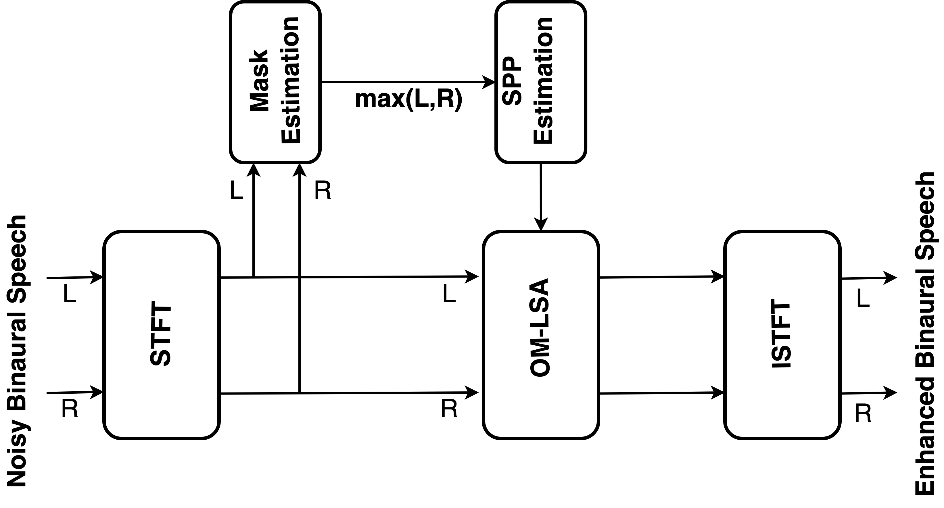
Fig. 1: Block diagram of the proposed method.

A block diagram of the proposed method is shown in Fig 1. The L and R labels indicate the left and right channels of a binaural signal. The left and right channels are processed in parallel for all stages of the algorithm. The noisy binaural signal is transformed into the STFT domain for TF-based processing. From the STFT domain signals, 3 feature subsets as defined in Sec. 2.2.1 are extracted once per STFT frame and the same features are used for the training and prediction stages of the algorithm. STOI optimal masks correlate to intelligible speech in the signal and SPP is computed from the estimated continuous-valued mask and then supplied to the OM-LSA. The output signal of the OM-LSA is transformed back into to the time-domain by applying an Inverse STFT (ISTFT).

2.2.1 Mask Estimation Features

The feature extraction and mask estimation follows the method from [18]. The first step in feature extraction for mask estimation is to normalize the noisy speech active level to 0 dB using the ITU P.56 objective speech active level [19] to make the algorithm level independent. Each of the three feature subsets has $\Psi$ features, giving $3\Psi$ features in total.

The first feature subset is constructed from the TF gains estimated by the Log-MMSE speech enhancement algorithm [20, 21], that minimizes the mean-squared error in the log-spectral amplitudes. The TF gains are expected to be high when speech is present and low otherwise. As this algorithm uses a noise estimator [22], these features are expected to help generalize the mask estimator to unseen noise types. The gain function $G(k,m)$ from [20] satisfies $G(k,m)|Y(k,m)|=\mathrm{exp}\{\mathbb{E}[\textrm{log}|X(k,m)|\;|Y(k,m)|]\}$ where, $\mathbb{E[.]}$ is the expectation operator. The first subset of features, $\boldsymbol{\mu}_{m}^{(1)}=\left[\mu_{1,m}^{(1)},...,\mu_{\Psi,m}^{(1)}\right]^{T}$, is a $\Psi\times 1$ vector found by averaging $G(k,m)$ in $\Psi=30$ triangular windows, $w_{i}(k)$ for $i=1,..,\Psi$ equally spaced on Equivalent Rectangular Bandwidth (ERB) scale centre frequencies and then computing the natural logarithm. For frame $m$, the feature subset is given by

$$\mu_{i,m}^{(1)}=\textrm{ln}\left\{\frac{\sum_{k=0}^{K/2}w_{i}(k)G(k,m)}{\sum_{k=0}^{K/2}w_{i}(k)}\right\}\textrm{for}\;i=1,...,\Psi$$ (5)

where $K$ is the Discrete Fourier Transform (DFT) length. The second feature subset, denoted by $\boldsymbol{\mu}_{m}^{(2)}=\left[\mu_{1,m}^{(2)},...,\mu_{\Psi,m}^{(2)}\right]^{T}$, is the estimate of the level-normalized enhanced speech amplitude in each frequency band and is obtained by multiplying the gains from the first feature subset with the noisy speech. The third feature subset $\boldsymbol{\mu}_{m}^{(3)}=\left[\mu_{1,m}^{(3)},...,\mu_{\Psi,m}^{(3)}\right]^{T}$ is an estimate of the local Voiced-Speech-plus-Noise to Noise Ratio (VSSNR) in the TF regions and is obtained using the PEFAC algorithm [23]. The fundamental frequency of the speech in each frame is computed and then VSSNR is estimated within the $\Psi$ frequency bands by comparing the energy at harmonics of the fundamental frequency with the energy halfway between consecutive harmonics. The complete feature set for frame $m$ is obtained by concatenating the three subsets to obtain the feature set $\boldsymbol{\mu}_{m}=\left[\boldsymbol{\mu}_{m}^{(1)T},\boldsymbol{\mu}_{m}^{(2)T},\boldsymbol{\mu}_{m}^{(3)T}\right]^{T}$.

2.2.2 Target Mask and Deep Neural Network (DNN)

The difference between SOBM and HSWOBM is that the latter is designed to optimize WSTOI rather than STOI and is computed over a higher number of frequency bands (129 instead of 15) to increase the resolution of the mask. In the proposed method, HSWOBMs are used as target masks and are computed using the three-stage dynamic programming technique described in [13] which consists of carrying out three passes of estimation with a pruning strategy to compute the target masks to optimise the WSTOI from (4). Directional white Gaussian noise at 0 dB SNR is added to binaural speech signals to generate the training data and computation of target masks. The target masks are computed for the left and right channels individually based on the speech content in each channel. The HSWOBM is computed by forming a masked signal $Z_{j}(m)=B_{j}(m)Y_{j}(m)$ where $B_{j}(m)\in\{0,1\}$. The clipped modulation masked vector $\mathbf{\tilde{z}}_{j,m}$ is then computed analogous to (2) to limit the impact of frames having low speech energy. $B_{j}$ is numerically optimized using least squares method separately in each band, $j$, by computing

$$B_{j}(m)=\operatorname*{arg\,max}_{\{B_{j}(m):m=1,...,N\}}\left(\sum_{m=1}^{N}I_{j,m}\mathbb{E}[d(\mathbf{x}_{j,m},\mathbf{\tilde{z}}_{j,m})]\right)$$

where $N$ is the number of frames and

$$\mathbb{E}[d(\mathbf{x}_{j,m},\mathbf{\tilde{z}}_{j,m})]\approx\frac{(\mathbf{x}_{j,m}-\bar{x}_{j,m})^{T}\;\mathbb{E}[\mathbf{\tilde{z}}_{j,m}]}{\lVert\mathbf{x}_{j,m}-\bar{x}_{j,m}\rVert\;\sqrt{\vrule height=12.0pt,depth=3.60004pt,width=0.0pt\mathbb{E}[\lVert\mathbf{\tilde{z}}_{j,m}-\bar{\tilde{z}}_{j,m}\rVert^{2}}]}.$$ (6)

A feed-forward DNN is trained to estimate a continuous mask from the features extracted from the noisy binaural signals by using the HSWOBM target masks estimated by dynamic programming [13, 18]. The DNN consists of 4 layers of ‘dense’ or ‘fully-connected’ layers each with 500 hidden neurons. Rectified Linear Unit (ReLU) is used as the activation function for all the layers except the output layer where the Sigmoid activation function is used. Dropout layers are placed between the layers with a dropout factor of 20%. A weighted mean square error is used as the cost function for the DNN. The cost function, $\mathcal{J}$, is given by

$$\mathcal{J}=\frac{1}{\Delta}\frac{\sum_{p=1}^{\Delta}\phi_{p}(\mathrm{c}_{p}-\zeta_{p})^{2}}{\sum_{p=1}^{\Delta}\phi_{p}}$$ (7)

where $c_{p}$ is the output of the DNN, $\Delta$ is the number of pairs of feature vectors and corresponding mask value pairs available for training, $\zeta_{p}$ is the training target and $\phi_{p}$ is the corresponding value of the weight. The weights are computed from the WSTOI sensitivity and band importance weighting obtained from the WSTOI metric [14].

2.2.3 Better-ear Processing

Studies [3, 10] have shown that human listeners are capable of better ear listening, which is focusing on the speech signal from the ear which has higher SNR and intelligibility. We adopt a similar approach in our method for the selection of the mask values or the gains in each TF bin. Choosing the maximum gain value from the two estimated masks for the left and right channels is equivalent to selecting the gain associated with lower noise levels and higher speech presence from the SPP estimation. In order to preserve the spatial cues of the binaural signal, the same gain needs to be applied to both the channels. Hence, in our method, we use the gains selected from the above method to compute a single SPP to input to the OM-LSA enhancer for both the channels.

2.2.4 Optimally Modified-LSA

Mask-application follows the method in [15], that is shown to improve the perceptual quality of masked speech. From the computed HSWOBM, an intermediate continuous-valued mask is estimated and, instead of applying this mask as a TF domain gain, it is used to supply the probability of speech presence to a speech enhancer [24] that minimizes the expected error in the Log Spectral Amplitude (LSA). Let us consider the hypothesis $H_{1}(k,m)$ in the $k^{th}$ bin where speech is present and $H_{0}(k,m)$ where speech is absent. Considering the gain $G(k,m)$ to be larger than a threshold $G_{min}$ when the speech is absent, it is shown in [24] that

$$G(k,m)=\{G_{H_{1}}(k,m)\}^{p(k,m)}\;G_{min}^{1-p(k,m)}$$ (8)

where $G_{H_{1}}(k,m)$ is the gain under the hypothesis $H_{1}(k,m)$ and $p(k,m)\triangleq P(H_{1}(k,m)|Y(k,m))$ is the conditional SPP and is given by

$$p(k,m)=\left\{1+\frac{q(k,m)}{1-q(k,m)}(1+\xi(k,m))\mathrm{exp}(-v(k,m))\right\}^{-1}$$

where $q(k,m)\leavevmode\nobreak\ \triangleq\leavevmode\nobreak\ P(H_{0}(k,m))$ is the a priori probability of speech absence in the hypothesis $H_{0}(k,m)$, $v(k,m)$ is the a posteriori SNR and $\xi(k,m)$ is the a priori SNR . In [15] it is shown that, by using the gain value of the mask to control the speech probability and using this to enhance the speech using OM-LSA, there is a soft imposition of the spectro-temporal modulations required to preserve the intelligibility of the enhanced speech. From the estimated better-ear continuous mask, the SPP which will be used to enhance both the channels is computed and supplied to the OM-LSA. The enhanced signals are then transformed into the time domain from the TF domain by performing the inverse STFT.

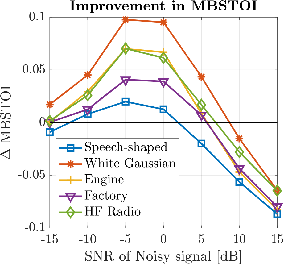
(a)

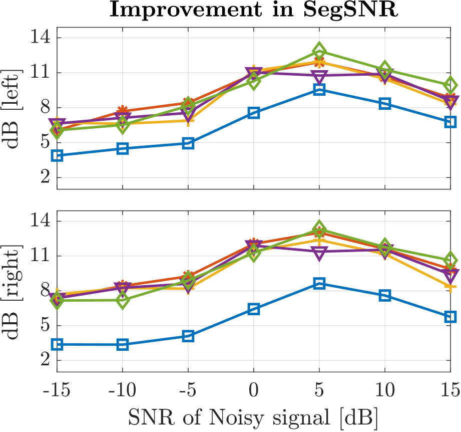
(b)

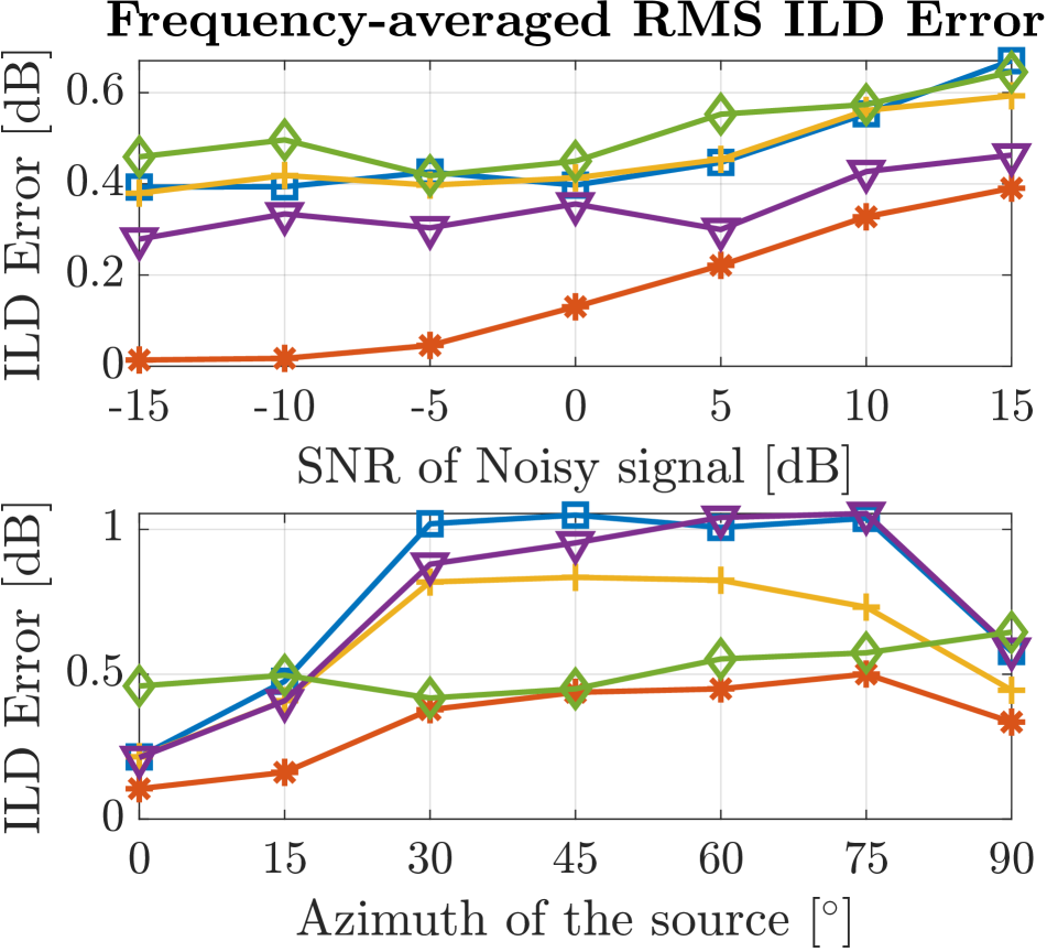
(c)

Fig. 2: (a) Improvement in MBSTOI score, (b) improvement in frequency weighted segmental SNR for both channels and (c)(upper) frequency averaged RMS ILD error with different SNRs, for a source placed 80 cm away at $30^{\circ}$ azimuth and noise at $0^{\circ}$ azimuth (c)(lower) frequency averaged RMS ILD error for source at 80 cm with 0 dB SNR for different azimuths of the source and the noise at $0^{\circ}$ azimuth.

3 Simulation Experiments

Simulations were performed using speech utterances from TIMIT [25] and noise signals from NOISEX-92 [26] and all signals were resampled to 10 kHz. To simulate binaural signals and directional noise, the Head Related Impulse Response (HRIRs) from [27] were used. To generate the training target HSWOBM masks, 400 speech signals from TIMIT and the anechoic in-ear HRIRs were used. The source azimuth was randomly selected between $-90^{\circ}$ and $+90^{\circ}$ with a resolution of $5^{\circ}$ and with elevation and distance fixed at 80 cm and $0^{\circ}$. The target masks for the left and right channels were then computed as described in Sec. 2.2.2. A feed-forward DNN was designed in Python using Tensorflow. Around 2 million trainable parameters were generated from the three extracted feature sets. The DNN was trained to estimate a continuous mask to optimize the WSTOI metric in each channel by minimizing the cost function in (7). The generated trainable data was split into 70% for training and 30% for validation while training the model. For evaluation, 30 unseen male and female speech utterances randomly selected from TIMIT test dataset, and 5 types of noise signals from NOISEX-92, and spatialized using HRIRs [27] were used to generate the test data.

Experiments with different SNRs were performed by adding a normalized directional noise at $0^{\circ}$ azimuth to a normalized binaural speech signal at SNRs in the range of -15 dB to +15 dB in steps of 5 dB. The A-weighted frequency segmental SNR [28, 21] is measured to show the noise reduction, MBSTOI [29] to show the binaural intelligibility improvement and the ILD error to quantify the preservation of binaural cues. The ILD for binaural signals is computed in each TF bin as $\textrm{ILD}_{(k,m)}=20\textrm{log}_{10}(|Y_{L}(k,m)|/|Y_{R}(k,m)|)$, where $Y_{L}$ and $Y_{R}$ are the left and right channel STFT domain signals. The RMS ILD error is computed by averaging the error over all the frequencies and for SNRs in the range of -15 dB to +15 dB in steps of 5 dB of received binaural speech and at azimuths 0 to $90^{\circ}$ in steps of $15^{\circ}$. The RMS ILD error was averaged over frequency because in our experiments no significant changes in the error were observed over frequencies. In both the experiments to compute the RMS ILD error, the directional noise was placed at $0^{\circ}$ azimuth. The proposed method does not alter the phase of the signal while processing and therefore ITDs of the enhanced signal will be the same as the signal before processing.

4 Results

Figure 2(a) shows the improvement in MBSTOI and maximum improvement was observed between -5 to 0  dB SNR for all noise cases. At very noisy SNRs of under -10 dB, extraction of speech features from the signal to estimate an accurate mask becomes difficult, which explains lower improvements. However, in Fig. 2(b), which shows the improvement in segmental SNR, even under very noisy cases of -15 dB SNR where the speech information in the extracted features is low, the method was able to provide at least 3 dB SNR improvement for all the noise cases and as the signal SNR improved, SNR improvements greater than 10 dB were also observed. For SNRs higher than 5 dB, there is negative improvement in MBSTOI, as the input binaural speech signal has a higher MBSTOI score before processing and applying mask based enhancement on these signals results in reducing the score. As all the signals above 5 dB SNR had a MBSTOI score above 0.7 after processing, the overall intelligibility of speech signals did not deteriorate to unintelligible levels. From Fig. 2(b), it can seen that a similar improvement in segmental SNR can be observed for all the noise cases with speech shaped noise being the exception and also from Fig. 2(a), lowest improvement for MBSTOI can be seen for speech shaped noise. Although speech shaped noise is a stationary noise, as it has most of its energy located in the TF bins shared with speech, thus impacting the estimation of SPP and hence the performance. For the experiments with multiple azimuth angles, the source was simulated at azimuths from $0^{\circ}$ to $90^{\circ}$ since the other half of the frontal plane in the HRIRs database [27] is a reflection of the former. Figure 2(c) shows the frequency averaged RMS ILD error observed with the method for input SNRs of the noisy signal and for different azimuth angles of the source. For all the noise cases, SNRs and azimuths the RMS ILD error observed is under 1 dB in the frontal plane. For all azimuths and SNRs, the proposed method performed the best for white Gaussian noise having the least error among all the noise cases. This low RMS ILD error after processing quantifies the binaural cue preservation of the method.

5 Conclusions

We have presented a new approach using STOI-optimal masking to enhance noisy binaural speech signals that not only improves the SNR but also preserves the interaural cues and intelligibility. Instead of applying the TF masks as a gain function, SPP is calculated and used by an OM-LSA speech enhancer. The proposed method is able to provide significant improvements in frequency weighted SNR, MBSTOI score and minimal distortion of interaural cues.

References

- [1] R. Beutelmann and T. Brand, “Prediction of speech intelligibility in spatial noise and reverberation for normal-hearing and hearing-impaired listeners,” J. Acoust. Soc. Am., vol. 120, p. 331, 2006.
- [2] M. Lavandier and J. F. Culling, “Prediction of binaural speech intelligibility against noise in rooms,” J. Acoust. Soc. Am., vol. 127, no. 1, pp. 387–399, Jan. 2010.
- [3] J. Blauert, Spatial Hearing: The Psychophysics of Human Sound Localization. Cambridge, MA, USA: The MIT Press, 1997.
- [4] M. L. Hawley, R. Y. Litovsky, and J. F. Culling, “The benefit of binaural hearing in a cocktail party: Effect of location and type of interferer,” J. Acoust. Soc. Am., vol. 115, no. 2, pp. 833–843, 2004.
- [5] T. Lotter and P. Vary, “Dual-channel speech enhancement by superdirective beamforming,” EURASIP J. on Applied Signal Process., vol. 2006, no. 1, pp. 1–14, 2006.
- [6] E. Hadad, D. Marquardt, S. Doclo, and S. Gannot, “Theoretical analysis of binaural transfer function MVDR beamformers with interference cue preservation constraints,” IEEE/ACM Trans. Audio, Speech, Language Process., vol. 23, no. 12, pp. 2449–2464, Dec. 2015.
- [7] E. Hadad, D. Marquardt, S. Doclo, and S. Gannot, “Binaural multichannel Wiener filter with directional interference rejection,” in Proc. IEEE Int. Conf. on Acoust., Speech and Signal Process. (ICASSP), Apr. 2015.
- [8] S. Doclo, T. J. Klasen, T. Van den Bogaert, J. Wouters, and M. Moonen, “Theoretical analysis of binaural cue preservation using multi-channel wiener filtering and interaural transfer functions,” in Proc. Int. on Workshop Acoust. Echo and Noise Control (IWAENC), 2006.
- [9] A. H. Moore, L. Lightburn, W. Xue, P. A. Naylor, and M. Brookes, “Binaural mask-informed speech enhancement for hearing aids with head tracking,” in Proc. Int. Workshop on Acoust. Signal Enhancement (IWAENC), Tokyo, Japan, Sep. 2018, pp. 461–465.
- [10] T. Green, G. Hilkhuysen, M. Huckvale, S. Rosen, M. Brookes, A. Moore, P. Naylor, L. Lightburn, and W. Xue, “Speech recognition with a hearing-aid processing scheme combining beamforming with mask-informed speech enhancement,” Trends in Hearing, vol. 26, Jan. 2022.
- [11] S. Gonzalez and M. Brookes, “Mask-based enhancement for very low quality speech,” in Proc. IEEE Int. Conf. on Acoust., Speech and Signal Process. (ICASSP), Florence, May 2014.
- [12] N. Li and P. C. Loizou, “Factors influencing intelligibility of ideal binary-masked speech: Implications for noise reduction,” J. Acoust. Soc. Am., vol. 123, no. 3, pp. 1673–1682, Mar. 2008.
- [13] L. Lightburn and M. Brookes, “SOBM - a binary mask for noisy speech that optimises an objective intelligibility metric,” in Proc. IEEE Int. Conf. on Acoust., Speech and Signal Process. (ICASSP), Apr. 2015, pp. 5078–5082.
- [14] L. Lightburn and M. Brookes, “A Weighted STOI Intelligibility Metric based on Mutual Information,” in Proc. IEEE Int. Conf. on Acoust., Speech and Signal Process. (ICASSP), Mar. 2016.
- [15] L. Lightburn, E. De Sena, A. H. Moore, P. A. Naylor, and M. Brookes, “Improving the perceptual quality of ideal binary masked speech,” in Proc. IEEE Int. Conf. on Acoust., Speech and Signal Process. (ICASSP), Mar. 2017.
- [16] C. H. Taal, R. C. Hendriks, R. Heusdens, and J. Jensen, “An algorithm for intelligibility prediction of time-frequency weighted noisy speech,” IEEE Trans. Audio, Speech, Language Process., vol. 19, no. 7, pp. 2125–2136, Sep. 2011.
- [17] R. Kneser and H. Ney, “Improved backing-off for M-gram language modeling,” in Proc. (IEEE) Intl. Conf. on Acoustics, Speech and Signal Processing (ICASSP), vol. 1, May 1995, pp. 181–184 vol.1.
- [18] L. Lightburn, “Mask-based enhancement of very noisy speech,” Ph.D. dissertation, Imperial College London, 2020.
- [19] “P. 56: Objective measurement of active speech level,” Int. Telecommun. Union (ITU-T), Recommendation, Mar. 1993.
- [20] Y. Ephraim and D. Malah, “Speech enhancement using a minimum mean-square error log-spectral amplitude estimator,” IEEE Trans. Acoust., Speech, Signal Process., vol. 33, no. 2, pp. 443–445, 1985.
- [21] D. M. Brookes, “VOICEBOX: A speech processing toolbox for MATLAB,” 1997. [Online]. Available: http://www.ee.ic.ac.uk/hp/staff/dmb/voicebox/voicebox.html
- [22] T. Gerkmann and R. C. Hendriks, “Unbiased MMSE-based noise power estimation with low complexity and low tracking delay,” IEEE Trans. Audio, Speech, Language Process., vol. 20, no. 4, pp. 1383–1393, May 2012.
- [23] S. Gonzalez and D. M. Brookes, “PEFAC - A pitch estimation algorithm robust to high levels of noise,” IEEE/ACM Trans. Audio, Speech, Language Process., vol. 22, pp. 518–530, Feb. 2014.
- [24] I. Cohen, “Optimal speech enhancement under signal presence uncertainty using log-spectral amplitude estimator,” IEEE Signal Process. Lett., vol. 9, no. 4, pp. 113–116, Apr. 2002.
- [25] J. S. Garofolo, L. F. Lamel, W. M. Fisher, J. G. Fiscus, D. S. Pallett, N. L. Dahlgren, and V. Zue, “TIMIT acoustic-phonetic continuous speech corpus,” Linguistic Data Consortium (LDC), Philadelphia, USA, Corpus LDC93S1, 1993.
- [26] A. Varga and H. J. M. Steeneken, “Assessment for automatic speech recognition II: NOISEX-92: A database and an experiment to study the effect of additive noise on speech recognition systems,” Speech Commun., vol. 3, no. 3, pp. 247–251, Jul. 1993.
- [27] H. Kayser, S. D. Ewert, J. Anemüller, T. Rohdenburg, V. Hohmann, and B. Kollmeier, “Database of multichannel in-ear and behind-the-Ear head-related and binaural room impulse responses,” EURASIP J. on Advances in Signal Process., vol. 2009, no. 1, p. 298605, Jul. 2009.
- [28] Y. Hu and P. C. Loizou, “Evaluation of objective measures for speech enhancement,” in Proc. Conf. of Int. Speech Commun. Assoc. (INTERSPEECH), 2006, pp. 1447–1450.
- [29] A. H. Andersen, J. M. de Haan, Z. H. Tan, and J. Jensen, “Refinement and validation of the binaural short time objective intelligibility measure for spatially diverse conditions,” Speech Commun., vol. 102, pp. 1–13, Sep. 2018.