The 700 ks Chandra Spiderweb Field II: Evidence for inverse-Compton and thermal diffuse emission in the Spiderweb galaxy

Abstract

Aims. We present the X-ray imaging and spectral analysis of the diffuse emission around the radio galaxy J1140-2629 (the Spiderweb galaxy) at $z=2.16$ and of its nuclear emission, based on a deep (700 ks) Chandra observation.

Methods. We obtained a robust characterization of the unresolved nuclear emission, and carefully computed the contamination in the surrounding regions due to the wings of the instrument point spread function. Then, we quantified the extended emission within a radius of 12 arcsec. We used the Jansky Very Large Array radio image to identify the regions overlapping the jets, and performed X-ray spectral analysis separately in the jet regions and in the complementary area.

Results. We find that the Spiderweb galaxy hosts a mildly absorbed quasar, showing a modest yet significant spectral and flux variability on a timescale of $\sim 1$ year. We find that the emission in the jet regions is well described by a power law with a spectral index of $\Gamma\sim 2-2.5$, and it is consistent with inverse-Compton upscattering of the cosmic microwave background photons by the relativistic electrons. We also find a roughly symmetric, diffuse emission within a radius of $\sim 100$ kpc centered on the Spiderweb galaxy. This emission, which is not associated with the jets, is significantly softer and consistent with thermal bremsstrahlung from a hot intracluster medium (ICM) with a temperature of $kT=2.0_{-0.4}^{+0.7}$ keV, and a metallicity of $Z<1.6\,Z_{\odot}$ at 1 $\sigma$ c.l. The average electron density within 100 kpc is $n_{e}=(1.51\pm 0.24\pm 0.14)\times 10^{-2}$ cm^-3, corresponding to an upper limit for the total ICM mass of $\leq(1.76\pm 0.30\pm 0.17)\times 10^{12}M_{\odot}$ (where error bars are $1\sigma$ statistical and systematic, respectively). The rest-frame luminosity $L_{0.5-10{\rm keV}}=(2.0\pm 0.5)\times 10^{44}$ erg s^-1 is about a factor of 2 higher than the extrapolated $L-T$ relation for massive clusters, but still consistent within the scatter. If we apply hydrostatic equilibrium to the ICM, we measure a total gravitational mass $M(<100\leavevmode\nobreak\ {\rm kpc})=(1.5^{+0.5}_{-0.3})\times 10^{13}\,M_{\odot}$ and, extrapolating at larger radii, we estimate a total mass $M_{500}=(3.2^{+1.1}_{-0.6})\times 10^{13}\,M_{\odot}$ within a radius of $r_{500}=(220\pm 30)$ kpc.

Conclusions. We conclude that the Spiderweb protocluster shows significant diffuse emission within a radius of 12 arcsec, whose major contribution is provided by inverse-Compton scattering associated with the radio jets. Outside the jet regions, we also identified thermal emission within a radius of $\sim 100$ kpc, revealing the presence of hot, diffuse baryons that may represent the embryonic virialized halo of the forming cluster.

1 Introduction

Protoclusters are defined as overdense regions in the high-$z$ Universe which are predicted to evolve into massive, virialized clusters of galaxies by $z=0$ (see Overzier, 2016, for a review). Identifying and studying their properties is key to studying the formation and evolution of the large-scale structure of the Universe. In particular, in recent years the scientific community has mostly focused on the identification of the first virialized, dark-matter-dominated halos, on the origin and evolution of the hot, diffuse baryons permeating the potential wells – the intracluster medium (ICM) – and on the transformational processes that affect star formation and nuclear activity in the member galaxies. From the observational point of view, a protocluster is usually identified as a high-z region that is overdense in galaxy counts compared to the field. However, the dynamical state of the structure and the virialized mass that its halo ultimately achieves by $z=0$ is usually highly uncertain (see, e.g., Muldrew et al., 2015). At present, there are no standard methods to search for protoclusters, and this is the reason why biased-tracer techniques are often used to identify promising candidates. For example, several protoclusters have been found around high redshift, powerful radio galaxies. Spectroscopic follow-up has provided evidence that a significant fraction of powerful, high-z radio galaxies reside in a protocluster or overdense regions (see Venemans et al., 2007; Galametz et al., 2012; Wylezalek et al., 2013). In addition to massive spectroscopic surveys, intensive multiwavelength campaigns in the radio and X-ray bands are necessary to trace the many processes occurring in the protocluster member galaxies during their rapid evolution, such as nuclear activity, feedback into the surrounding medium, star formation, chemical enrichment, among others.

In this paper we focus on the role of deep X-ray observations. X-ray data are unique to use when studying the unresolved emission from active galactic nuclei (AGN), due to the accretion onto nuclear supermassive black holes (SMBHs), the thermal diffuse emission from the ICM, and the inverse-Compton (IC) emission from relativistic plasma. To a lesser extent, X-ray observations can also be used to trace the less intense emission from strongly star-forming galaxies, but this signal is too weak to be detected beyond $z\sim 1.5$ (see, e.g., Lehmer et al., 2016). Until now, only a few deep ($t_{\rm exp}\geq 200$ ks) observations of protoclusters have been carried out with Chandra or XMM-Newton. While the unresolved emission from AGN is relatively easy to detect, the faint, extended emission associated with the expected proto-ICM has been very hard to detect, with a few promising candidates (Gobat et al., 2011; Valentino et al., 2016; Wang et al., 2016), and some other cases where it is not possible to determine the thermal or relativistic nature of the diffuse emission unambiguously (Gilli et al., 2019; Champagne et al., 2021). This is not surprising since the expected thermal emission from $z\gtrsim 2$ protoclusters is predicted to be very faint from semianalytic models and numerical simulations (see Saro et al., 2009). In addition, the presence of nonthermal diffuse emission associated with the relativistic electrons in the radio jets, coupled to the bright, unresolved nuclear emission from protocluster members, which are both often present, may easily overwhelm the thermal emission from the proto-ICM. This implies that only high-sensitivity and angular-resolution ($\sim 1$ arcsec) observations can be used to search and characterize the diffuse, thermal emission in high-z protocluster and, at the same time, the unresolved emission from AGN members and the diffuse, nonthermal emission due to IC from radio jets.

A key piece of information in protoclusters is the identification and characterization of thermal emission from surrounding diffuse baryons, which directly traces the thermodynamics of the largest baryonic component and, at the same time, the virialization status of the halo. As of today, there have been no observations that can track the origin of the ICM from the birth of the protocluster, to the formation of an evolved, virialized clusters. In this short yet intense phase, which is expected to occur in the redshift range $2<z<3$, the heating of the proto-ICM can be due to several mechanisms, namely the following: accretion shocks; heating from stellar winds associated with strong star formation episodes in the protocluster galaxies; and mechanical heating and turbulence caused by radio jets from the central massive galaxy. Therefore, a characterization of the proto-ICM, including its morphology, thermodynamical, and chemical properties, can provide an independent and direct measure of the heating efficiency of the feedback and of the gas accretion and circulation into the protocluster potential well. In addition, feedback processes not only affect the ICM, but can also couple directly with the member galaxies, as suggested by the recent X-ray observation of a $z\sim 1.7$ protocluster (Gilli et al., 2019).

In this paper we investigate the diffuse emission (both thermal and nonthermal) and the central nuclear emission of the Spiderweb galaxy (J1140-2629) protocluster at $z=2.16$, using a deep Chandra ACIS-S observation ($\sim 700$ ks). The central, powerful radio galaxy is embedded in a giant Ly$\alpha$ halo (Pentericci et al., 1997; Miley et al., 2006), and surrounded by a $\gtrsim 2$ Mpc–sized overdensity of star-forming galaxies (Ly$\alpha$ and H$\alpha$ emitters), dusty starbursts, and galaxies that are rapidly migrating toward a nascent red sequence (Zirm et al., 2008). The archetypal Spiderweb protocluster is expected to evolve into a massive cluster in less than 1.5 Gyr, with the radio galaxy itself showing the properties of a cD progenitor (Miley et al., 2006). In a companion paper (Tozzi et al., 2022, hereafter Paper I), we investigated the nuclear activity in the protocluster members, finding a high fraction of bright AGN with $L_{0.5-10keV}>3\times 10^{43}$ erg s^-1 in spectroscopically confirmed members with ${\rm log}(M_{*}/M_{\odot})>10.5$, equal to $25.5\pm 4.5$%, and estimating an enhancing factor of $6.0^{+9.0}_{-3.0}$ for the nuclear activity with respect to the COSMOS field at comparable redshifts and stellar mass range. Here we focus on the very central regions of the Spiderweb protocluster, which is a rapidly evolving, high-density region where complex and intricate phenomena concur to shape the properties of the nascent brightest cluster galaxy (BCG) and possibly an embryonic ICM halo. Such diffuse X-ray emission is also investigated in connection with the radio (JVLA) and submillimeter (ALMA) spatially resolved signal in other papers of the collaboration (Carilli et al., 2022; Anderson et al., 2022, Di Mascolo et al. in preparation). Finally, in a forthcoming paper, the structure and thermodynamics of the ICM will be investigated by combining X-ray and submillimeter data (Lepore et al. in preparation).

The paper is organized as follows. In Section 2 we summarize the properties of the Spiderweb galaxy and its immediate surroundings on the basis of previous multiwavelength observations. In Section 3 we briefly recall the X-ray data acquisition and reduction, which has already been detailed in Paper I. In Section 4 we present the ray-tracing simulations we used to accurately model the unresolved nuclear emission, a step needed to estimate the contamination of the AGN to the extended emission and, therefore, exploit the imaging capability of Chandra when studying the morphology of such emission. In Section 5 we present a detailed analysis of the nuclear emission, including its variability. In Section 6 we finally investigate the nature of the diffuse X-ray emission surrounding the Spiderweb galaxy, spatially separating the thermal and nonthermal contribution. In Section 7 we focus on the nature of the thermal diffuse component, and discuss the implication of the presence of a virialized halo. Finally, our conclusions are summarized in Section 8. Throughout this paper, we adopt the seven-year Wilkinson Microwave Anisotropy Probe cosmology with $\Omega_{\Lambda}=0.73$, $\Omega_{m}=0.27$, and $H_{0}=70.4$ km s^-1 Mpc^-1 (Komatsu et al., 2011). In this cosmology, at $z=2.156$, 1 arcsec corresponds to 8.473 kpc, the Universe is 3.13 Gyr old, and the lookback time is 77% of the age of the Universe. Therefore, the size of a Chandra ACIS pixel (0.492 arcsec) corresponds to $4.237$ kpc. These values are especially relevant in the following section where we interchangeably report distances in pixels, arcsecs, or kiloparsecs. Quoted error bars correspond to a 1 $\sigma$ confidence level, unless noted otherwise.

2 The Spiderweb galaxy: Previous observational campaign and main results

The Spiderweb Galaxy (J1140-2629) and its environment have been extensively targeted in the last 25 years, with 54 papers published about the Spiderweb field including observations in radio, sub-mm, infra red (IR), optical and X–ray wavelengths. In this section we summarize the main results that have been obtained on the Spiderweb Galaxy focusing on its immediate environment, while a review on the properties of the protocluster galaxy population has been presented in Paper I. In the last subsection we point out the open science cases that are addressed by this work.

2.1 Discovery and peculiarities

The Spiderweb Galaxy was identified as a high-z radio galaxy (HzRG) while targeting ultra-steep spectrum radio sources (Roettgering et al., 1994) in an ESO Key Program. The peculiarity of this object was immediately noticed thanks to the unusually clumpy and bent radio morphology, and the exceptionally high rotation measure ($\sim 6200$ rad/m), showing that the radio synchrotron jet is severely affected by a surrounding, dense ($10^{-1}-10^{-2}$cm^-3) external medium (Carilli et al., 1997; Pentericci et al., 1997; Athreya et al., 1998). From the optical point of view, the Spiderweb Galaxy has been classified as a narrow emission line galaxy at $z=2.16$ (see Roettgering et al., 1997). A clumpy morphology has been observed also in the optical band, and HST ACS observations revealed that this is due to $\sim 10$ star-forming satellite galaxies moving with peculiar velocities of several hundred km s^-1, with a distribution resembling that of flies trapped in a spiderweb (Miley et al., 2006), and probably in the process of merging with the central radio galaxy within a few hundreds of Myr. Nevertheless, the most striking feature is constituted by a spectacular 200 kpc Ly$\alpha$ halo with a luminosity of $42.5\times 10^{44}$ erg s^-1 elongated along the direction of the jets. The total stellar mass inferred from the K-band luminosity is $10^{12}M_{\odot}$ (Pentericci et al., 1997), and it has been confirmed by Spitzer data (Seymour et al., 2007). The large majority of the stellar mass appears to be already in place well before $z=2.16$, while the satellite galaxies have measured stellar masses in the range $10^{8}<M_{*}<10^{10}M_{\odot}$, contributing only $\sim 1/10$ of the total mass of the central galaxy.

The optical and NIR spectrum of the nucleus of J1140-2629 shows a broad, spatially unresolved H$\alpha$ line (blended with [NII]) with a FWHM of $\sim 14900$ km s^-1 (Nesvadba et al., 2011). The presence of broad nuclear lines is rare for optical counterparts of high redshift radio sources, which typically show narrow emission lines and are classified as TypeII AGN. Other emission lines which have been detected include [OII], [NeIII], H_β narrow, [OIII], [OI], [NII], [SII], and a strong CIV and HeII (see Humphrey et al., 2008). Such an optical spectrum is consistent with photoionization from the AGN, powered by a SMBH with estimated mass $M_{BH}=2\times 10^{10}M_{\odot}$, putting J1140-2629 a factor of $\sim 2$ above the local $M-\sigma$ relation (Nesvadba et al., 2011).

Taken together, the observed characteristics suggest that the Spiderweb is indeed a massive radio galaxy forming at the center of a dynamically evolving protocluster region, that is likely to evolve into a BCG (see Pentericci et al., 1997). These findings sparkled a wide interest in this object and its surroundings, as one of the most promising targets where the evolutionary transition from a collapsing large scale structure to a gravitationally bound halo heavily affects the entire galaxy population.

2.2 Star formation activity in and around J1140-2629

The Spiderweb Galaxy shows a star formation rate of $15.6\pm 0.7M_{\odot}$/yr from dust-uncorrected optical/UV emission, as opposed to a total of $\sim 50M_{\odot}$/yr contributed from all the ”flies” (Hatch et al., 2009). IR observations with Spitzer (De Breuck et al., 2010), Herschel and LABOCA (Seymour et al., 2012) provide, however, a different picture, finding that the contribution to the $8-1000\mu\,$m luminosity is $1.17\pm 0.27\times 10^{13}L_{\odot}$ and $0.79\pm 0.09\times 10^{13}L_{\odot}$ for an AGN and a starburst component, respectively. This implies a 20% Eddington accretion rate onto the SMBH and, most important, a star formation rate (SFR) equal to $1390\pm 150M_{\odot}$/yr, dramatically higher than the value derived from the UV/optical rest-frame. Such a large value is confirmed by other works based on spectroscopic analysis of IR data (Ogle et al., 2012; Rawlings et al., 2013), and it cannot be reconciled with the dust-corrected estimate based on the rest-frame UV and the simplistic assumption of a uniform dust screen by Hatch et al. (2008), implying that most of the star formation in the Spiderweb must be highly obscured at rest-UV wavelengths.

The diffuse UV-continuum light surrounding the Spiderweb Galaxy shows a distribution similar to the $Ly\alpha$ halo, and it is likely due to a young stellar population (Hatch et al., 2008) originated by a diffuse, in situ star formation of $57\pm 8\,M_{\odot}$/yr, or $\sim 140\,M_{\odot}$/yr if corrected by dust extinction. This interpretation is not free from complexities, though. The presence of CIV and HeII emission lines suggest an ionization source harder than stellar continuum, implying a lower limit of only $\sim 7$% of the $Ly\alpha$ emission associated with star formation (Hatch et al., 2008).

A key point here is the presence of a large gas reservoir that feeds both the central and the diffuse star formation. The molecular gas mass inferred from observation of the redshifted CO(1-0) line with ATCA (Emonts et al., 2013) is $M_{H_{2}}=6\times 10^{10}M_{\odot}$ (for $M_{H2}/L^{{}^{\prime}}_{CO}=0.8$). This reservoir is able to sustain a SFR of $\sim 1400M_{\odot}/$yr for only $\sim 40$ Myr, while the doubling-mass time would be as long as 0.8 Gyr. A deeper ATCA observation (Emonts et al., 2016), coupled with JVLA, was able to identify an even larger amount of molecular gas $M_{H_{2}}=1.5\pm 0.4\times 10^{11}M_{\odot}$ (assuming $\alpha_{CO}=4\,M_{\odot}$ (K km s^-1 pc²)^-1), associated with the $Ly\alpha$ halo, showing that there is enough molecular gas to fuel the star formation within the IGM up to $z\sim 1.6$.

Summing the $3\times 10^{9}M_{\odot}$ in ionized gas found by Nesvadba et al. (2006), the gas masses of various components of the ISM are about an order of magnitude lower than the stellar mass, suggesting that this is already quite an evolved galaxy with a gas fraction in line for a main sequence galaxy at $z\sim 2$. Again, this suggests that we might be witnessing a transition from a very active starburst phase triggered by a merging event to a radio-feedback dominated phase, leading to the more quiescent existence of a BCG.

How this transition will be happening is still very much debated and unclear. On the one hand we have the expectation that this transition should be short lived, and that strong nuclear activity is indeed able to rapidly quench star formation, to be consistent with the lack of bright IR sources at X-ray luminosities comparable to the Spiderweb ($L_{X}>10^{45}$ erg s^-1) in the GOODS-North deep field (Page et al., 2012). On the other hand, results obtained with improved statistics (Harrison et al., 2012), and actually extending a trend well established at lower X-ray luminosities, seem to suggest that high-accretion, X-ray luminous, nuclear activity phases do not show any obvious impact on the star formation rate and stellar mass growth of the host galaxies and that super massive black hole and galaxy growth rather coexist over cosmic times. In this perspective, it is key to investigate a large sample of massive, high-z transitional galaxies similar to the Spiderweb to assess the relative contribution of radiative and mechanical feedback.

2.3 Diffuse gas and feedback effects in the halo of J1140-2629

The X-ray band is a promising spectral window to explore the Spiderweb, particularly when considering the expected X-ray brightening of high-z radio galaxies driven by the cosmic microwave background (CMB) photons (see Hodges-Kluck et al., 2021). The discovery of extended X-ray emission, that was not possible to constrain in an early ROSAT HRI image (Carilli et al., 1998), was measured to reach a luminosity of $\sim 3\times 10^{44}$ erg s^-1 in the 2-10 keV band aligned along the direction of the jet on a scale of $\sim 20$ arcsec, thanks to the first shallow Chandra exposure of about $\sim 30$ ks (Carilli et al., 2002). From these preliminary data it was not possible to spectrally verify whether the dominant emission mechanism is thermal bremsstrahlung from hot gas or Inverse Compton due to a relativistic electron population.

The nature of the diffuse X-ray emission is clearly a key ingredient in any picture aimed at constraining the presence of a virialized halo and the feedback processes in the diffuse medium around the Spiderweb Galaxy. Nevertheless, signatures of preheating have been searched for at other wavelengths. Integral field unit spectroscopy with SPIFFI (SINFONI) at VLT, found evidences for strong outflows with velocities on the order of $\sim 2000$ km s^-1, and total kinetic power in the range $2\times 10^{46}$-$3\times 10^{47}$erg s^-1 (Nesvadba et al., 2006, 2011). The high ratio of kinetic over radiative power may indicate that J1140-2629 is about to complete the transition to the radio-mode feedback regime (see Fabian, 2012). This picture is reinforced by the gas kinematics derived from the [OIII]$\lambda 5007$ line, that highlights a structure reminiscent of ”bubbles” intended as expanding spheres or conical outflows (Humphrey et al., 2008), implying a relatively efficient interaction between the AGN and the interstellar medium. With a sufficient coupling, the jet has enough energy to totally remove the ISM of the host within $\sim 5\times 10^{8}$ yr.

2.4 Dynamical state of the Spiderweb Complex

A first dynamical estimate of the total mass from the member galaxy velocity dispersion provided a value of $\sim 2.3\times 10^{14}M_{\odot}$, contributed by two subgroups of $1.7$ and $0.6\times 10^{14}M_{\odot}$ and virial radii of 1.1 and 0.8 Mpc, respectively, assuming they are both virialized (Kurk et al., 2004). However, the entire system, as well as the two subgroups separately, seem far from being virialized, not only for the lack of evident extended, thermal X-ray emission, but also for the lack of a well-formed red-sequence in the J-K vs K color magnitude diagram (despite this does not necessarily follow or precede virialization). Thanks to near-infrared spectroscopy with SINFONI at VLT, Kuiper et al. (2011) found that the velocity distribution within 60 kpc of the Spiderweb Galaxy is consistent with bimodality, with no global peak resembling that of a virialized halo. They described the system as the merger of two halos that would predict, in case of virialization of both subhalos, a rest-frame 2-10 keV luminosity of $2\times 10^{43}$ erg s^-1. Finally Shimakawa et al. (2014) identified a region possibly virialized with a $R_{200}\sim 0.53$ Mpc and $\sigma_{cl}\sim 680$ km s^-1, while the inclusion of all the spectroscopic members would give $\sigma_{cl}\sim 880$ km s^-1, reflecting some velocity structures particularly in the outer regions. The inferred mass is consistent with that of a progenitor of present-day most massive class of galaxy clusters.

Saro et al. (2009) analyzed at $z=2.2$ cosmological hydrodynamical simulations of two protocluster regions, which form by $z=0$ two clusters with virial masses of $\sim 10^{14}$ and $\sim 10^{15}M_{\odot}$. The line-of-sight velocity dispersion of galaxies in the largest halo is roughly in agreement with the total observed dispersion in the Spiderweb Complex, thus suggesting that it is consistent with being the progenitor of a massive cluster by $z=0$ and that a diffuse atmosphere of hot gas already in equilibrium should be already present. Their prediction for the 0.5-2 keV flux from the ICM is $\sim 10^{-15}$ and $\sim 10^{-14}$ erg s^-1 cm^-2 for subhalo temperatures of 2 and 5 keV, respectively. These findings underline the importance of confirming the thermal nature of at least part of the diffuse X-ray emission around the Spiderweb Galaxy.

2.5 Open issues and role of the new X-ray observations

Previous works on the Spiderweb Complex found a clear overdensity in discrete source counts in all the observed bands, from sub-mm to the X-ray, that ranges from a factor of $\sim 2-6$ to $\sim 100$, depending on the source selection and on the specific region considered within the complex. In Paper I we explored the galaxy population of the Spiderweb Protocluster, finding an X-ray AGN fraction enhanced by a factor of $6.0^{+9.0}_{-3.0}$ with respect to the COSMOS field at comparable redshifts and stellar mass range.

In this work we focus on other key aspects concerning the Spiderweb Galaxy and its immediate surroundings: i) the nature of the diffuse emission; ii) the presence of diffuse thermal emission possibly associated with the virialization of a central halo; iii) the nuclear activity in the Spiderweb Galaxy. Exploring these aspects is mandatory to explore more general aspects concerning galaxy evolution, such as: the main process (gravitational or feedback) responsible for the heating of the proto-ICM; the compresence of hot and cold gas within the halo as a typical phase of the formation of BCG progenitors; the eventual evolution of the Spiderweb protocluster into a virialized structure by $z=0$. The new set of data obtained in the last couple of years in the Spiderweb field, and in particular the deep Chandra observation presented in this work, allows us to better address all the science goals listed here. The presence of hot, diffuse baryons around the Spiderweb Galaxy and its relation to its nuclear activity are discussed in other papers based on the combination of Chandra X-ray and JVLA Radio data (Carilli et al., 2022; Anderson et al., 2022). Moreover, the ICM of the Spiderweb Galaxy is also investigated with ALMA SZ data (Di Mascolo et al. in preparation). The main results and the data products can be found on the project webpage.

3 X-ray data reduction

The Spiderweb Galaxy was observed with a Chandra Large Program for 700 ks with ACIS-S granted in Cycle 20 (PI P. Tozzi). The observations were completed in the period November 2019 - August 2020, splitted in 21 separate Obsid. To this data set we add the first X-ray observation with ACIS-S, dating back to June 2000 for a total of 39.5 ks. All the Obsid are listed in Table 1 of Tozzi et al. (2021), where we also describe the followed standard data reduction procedure. We used the latest release of the Chandra Calibration Database at the time of writing (CALDB 4.9.3) We briefly recall that we run the task acis_process_events with the parameter apply_cti=yes to flag background events, most likely associated with cosmic rays, and, by rejecting them, obtain a significant reduction of the background, thanks to the VFAINT mode of data acquisition.

This step is particularly relevant in this work since the background may significantly affect the detection of the low surface-brightness, diffuse emission surrounding the Spiderweb Galaxy. The small price to pay is the removal of some of photons from bright sources. We find that slightly more than 100 net counts in the total band are removed at the position of the nucleus of J1140-2629 across the 22 exposures. This indicates that the source, which is by far the brightest in the field, suffers a small amount of pile-up. However, we have verified a posteriori that this effect does not impact the spectral analysis of the nucleus and therefore it is not worth to give up the VFAINT cleaning to recover less than 1% of the flux in the nucleus.

The final total exposure time after data reduction and excluding the dead-time correction amounts to 715 ks (corresponding to the LIVETIME keyword in the header of Chandra fits files), including the first observation. The 22 level-2 event files are merged together with the tool reproject_obs, using the reference coordinates of Obsid 21483. The soft (0.5-2 keV) and hard (2-7 keV) band images at full resolution in the immediate surroundings ($90\times 70$ arcsec²) of the Spiderweb Galaxy are shown in Figure 1. It is possible to notice the larger background in the hard band, and to appreciate the enhancement of the diffuse emission along the radio emission associated with the jets, shown with red contours (after Carilli et al., 2022). Fairly isotropic extended mission is also present far from the jets in the soft band. Clearly, a meaningful analysis of the extended emission must take into account all the complexity arising from the overlapping of four components: emission from the jets, isotropic extended emission, unresolved nucleus, and background. The choice of the extraction regions corresponding to different components is based on a detailed imaging analysis as described in the next Section. Finally, to perform spectral analysis, we extracted the spectra and computed the ancillary response file (ARF) and redistribution matrix file (RMF) for each observation separately with the command mkarf and mkacisrmf. Our default spectral analysis uses a local background that, given the small extent of the sources, is directly extracted from a source-free region on the same CCD-7 chip.

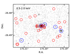
Figure 1: Close-up of the Spiderweb Galaxy ($90\times 70$ arcsec by side) at full angular resolution, in the soft (0.5-2 keV, left) and hard (2-7 keV, right) band. Extended emission is clearly visible in both bands. Red contours show radio emission observed in the 10 GHz band with the JVLA (see Carilli et al., 2022) at levels of $0.03$, $0.2$, $2$ and $20$ mJy/beam. It is possible to appreciate the larger background in the hard band, and the enhancement of the diffuse emission along the radio jets. Also, the extended emission appear to be stronger and more isotropic in the soft band. Blue circles correspond to X-ray emitting, spectroscopically confirmed members, while red circles to spectroscopically confirmed members with no X-ray emission (see Tozzi et al., 2022).

4 X-ray properties of the Spiderweb Galaxy: Imaging analysis

The X-ray images of the Spiderweb Galaxy show a prominent, dominant unresolved component due to the central AGN, and a clear diffuse emission limited to a radius of $\sim 12$ arcsec. Due to the brightness of the unresolved emission, the small extension and the composite nature of the diffuse emission, a detailed imaging and morphological analysis of the image is required to account for multiple components. The major contribution is due to the unresolved nucleus, that, due to its intensity, contaminates the surrounding regions up to radii of several arcsec. Therefore, as a first step, we perform ray-tracing simulations to obtain an accurate modalization of the unresolved AGN, assuming the same instrumental setup of the real data.

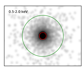
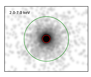
Figure 2: Simulated images of an unresolved source with the same observational characteristics (position, roll angle, exposure time and observation date) of the merged image of the Spiderweb Galaxy, in the 0.5-2 keV (left) and 2-7 keV (right) band. The inner red circle (2 arcsec radius) is used to extract the AGN spectrum, while the outer green circle (12 arcsec radius) encompasses the diffuse emission. The color scale is the same on both bands.

4.1 Ray-tracing simulations

To perform accurate ray-tracing simulations, we used the Chandra Ray Tracer (Chart) tool. First, we created spectral files with Sherpa to reproduce the spectrum of the Spiderweb nucleus. The spectral fits were performed with Xspec 12.11.1 (Arnaud, 1996) for each Obsid in order to track possible fluctuations in the flux and spectral shape as well. To model the nuclear emission, we considered the emission in the extraction region within a radius of 2 arcsec, which is clearly dominated by the AGN, but it still may include some minor, unknown contribution from diffuse emission. Despite this, the background subtraction in this first step was computed simply rescaling the emission in an annulus with inner and outer radii of 3^′′ and 5^′′, respectively, centered on the nucleus. This background subtraction can be considered as an amenable approximation to the non-AGN component within 2 arcsec, and it is sufficient to obtain spectra accurate enough to compute the expected image of the point spread function (PSF), which has a mild dependence on the photon energy. The spectral fits of the AGN obtained in this first step are not discussed, and the detailed description of the spectral analysis, with all the components properly included, are presented in Section 5. Spectral analysis of the diffuse emission, both thermal and nonthermal, is presented in Section 6.

The best-fit spectral parameters of a power law emission with intrinsic absorption obtained for each Obsid are given as input for the image simulations. We perform 10 ray tracing simulations for each one of the 22 Obsid. We pay attention to normalize the exposure time of the simulations to the actual effective exposure time of each Obsid after data reduction. Eventually, we create the evt2 file corresponding to a given simulation with Marx. We merge the ten files of each Obsid to obtain an event file corresponding to an exposure $10\times$ larger than in the real data. Finally, we merge all the simulated Obsid by reprojecting the evt2 files onto the reference frame of Obsid 21483 as in the reduction of real data. We obtain the soft and hard band images of the simulated source directly from the reprojected and merged file, dividing the outcome by a factor of 10 to obtain an image with the same nominal exposure time, but a Poisson noise a factor of $\sim 3$ lower. The images of the merged PSF in the soft and hard bands are shown in Figure 2, where the extraction region is shown as a red circle (with a radius of 2 arcsec), while the approximate extent of the diffuse emission is shown as a green circle (with a radius of 12 arcsec). The color scale is the same in both bands. The large majority of the signal is within a radius of 2 arcsec, however the wings of the PSF contribute a significant fraction of the total intensity in the region between 2 and 12 arcsec, with the PSF having slightly more extended wings in the hard band. From the simulated image we can robustly estimate that in the soft band 94.8% of the source emission is within 2 arcsec, and 4.0% between 2 and 12 arcsec, while only 1.2% is beyond 12 arcsec. In the hard band these values are 91.7%, 5.2% and 3.1%, respectively. From a preliminary estimate, the counts contributed in our data (full exposure) by the AGN in the 2-12 arcsec region, where the diffuse emission dominates, amounts to $\sim 300$ net photons in the 0.5-7 keV band. Since we measure a total of $\sim 900$ net counts in the 0.5-7 keV band in the 2-12 arcsec region, this implies that a non-negligible fraction ($\sim 0.33$) of the diffuse signal is due to the wings of the AGN emission.

4.2 Reconstruction of the diffuse emission

The next step is to accurately normalize the simulated image to the actual nuclear emission. We note, in fact, that the normalization of the spectra used for the ray-tracing simulations, were based on an approximate background subtraction. Therefore, while we trust the distribution of the emission according to the combined PSF, the overall normalization can be offset by a few percent. While this translates in an almost negligible correction to the normalization of the AGN emission, it is very important to estimate the relation between the AGN normalization and the diffuse component expected in the inner circle of 2 arcsec (corresponding to $\sim 17$ kpc), for example, to infer the degree of ”cool coreness”. In both cases, we note that in this step we consider both thermal and nonthermal components in the extended emission, since it is impossible, without spectral analysis, to disentangle the two components.

Therefore, we proceed as follows. We measure the emission in an annulus with inner and outer radius of 3 and 5 arcsec, respectively, that would correspond to the standard choice in case of an isolated, unresolved sources (see Tozzi et al., 2001). Within this annulus we find 1.5% and 1.9% of the total emission from the nucleus in the soft and hard bands, respectively. In addition, we also estimate the instrumental (plus unresolved extragalactic X-ray background) from an annulus with inner and outer radius of 16 and 29.5 arcsec, respectively. This last region (from where two unresolved sources have been previously identified and removed) has negligible contribution from the extended emission and the AGN emission, if any. Therefore, we estimate the instrumental background per pixel as $b_{i}=B_{i}/A_{B}$, where $B_{i}$ is the photometry in the 16-29.5 arcsec annulus and $A_{B}$ is the area of the annulus. The surface brightness of the diffuse emission in the range 3-5 arcsec can be written as $d=[D-(A_{d}\times b_{i})-p_{d}\times S_{AGN}]/A_{d}$, where $D$ is the total photometry in the 3^′′-5^′′ annulus, $A_{d}$ the area of the annulus, and $p_{d}$ is the fraction of the actual total signal from the AGN falling in the annulus, (computed from the simulated PSF images). Finally, the total photometry of the nuclear emission is $S_{AGN}=[C_{AGN}-A_{AGN}\times b_{i}-n_{d}\times A_{AGN}\times d]/p_{AGN}$, where $C_{AGN}$ is the photometry in the 2 arcsec extraction region, $A_{AGN}$ is the area of the extraction region, and $p_{AGN}$ is the fraction of the AGN emission falling into the extraction region (computed again from the simulated PSF images). This system can be easily solved, apart from the unknown, free parameter $n_{d}$ that is defined as the ratio of the average surface brightness within a radius of 2 arcsec with respect to the average surface brightness in the range 3-5 arcsec. We use the parameter $n_{d}$ to quantify our ignorance on the surface brightness of the diffuse emission in the 2 arcsec extraction region in terms of multiple of the average surface brightness observed in the 3.5^′′-5^′′ annulus.

Since it is likely to have an increase in the central surface brightness with respect to the outer annulus, we expect $n_{d}\geq 1$. In the case of a strong, small-scale cooling flow the spectral shape may change on the scale of $\sim 1$ arcsec (corresponding to $\sim 8.5$ kpc), and, therefore, the parameter $n_{d}$ may be different in the soft and in the hard band. If we consider, as a reference, the strong cool-core cluster CL1415 at $z\sim 1$ (Santos et al., 2012), and the same physical regions we are using here, we find that the surface brightness in the inner region is 3.3 and 2.7 times larger than that in the annulus in the soft and hard bands, respectively. Despite the fact that CL1415 is a mature, massive cluster observed at much lower redshift, we adopt values in the range 1-6 for the parameter $n_{d}$, where $n_{d}=1$ correspond to a constant surface brightness, $n_{d}\sim 3.5$ correspond to a fully developed cool core, and $n_{d}\sim 6$ to an exceptionally peaked cool core.

We compute the total photometry of the AGN in the soft and hard bands as a function of the enhancement factor $n_{d}$, and use these values to normalize the simulated images and compare them with the real data. The elative normalization of the diffuse emission within a radius of 2 arcsec (the $n_{d}$ parameter), nevertheless, has a marginal impact on the AGN emission. In the soft band the uncertainty on the AGN normalization is at most 100 net counts for a strong cool core with $n_{d}=3$ and 200 net counts for an extreme cool core with $n_{d}=6$ (corresponding to a relative uncertainty of 1.8% and 3.5%, respectively). In the hard band the uncertainty is much less, due to the lower surface brightness measured on the 3^′′-5^′′ annulus. The hard-band net counts expected from the diffuse emission within 2 arcsec are in the range 8-15, corresponding to an uncertainty of 0.2%-0.4% in the normalization of the nuclear hard emission.

If we focus on the estimated flux from diffuse emission within 2 arcsec, we find that the energy flux associated with diffuse emission within a radius of 2 arcsec is $(1.17\pm 0.09)\times 10^{-15}\times(n_{d}/3)$ erg s^-1 cm^-2 and $(2.9\pm 0.4)\times 10^{-16}\times(n_{d}/3)$ erg s^-1 cm^-2 in the soft and hard (2-10 keV) bands, respectively. These values have been obtained using the conversion factors at the aimpoint listed in Table 3 of Paper I. The lower value in the hard band is due to the low hardness ratio of the emission measured in the 3^′′-5^′′ annulus, which is measured to be $HR=-0.85$, and it provides a first, preliminary hint that the diffuse emission may be dominated by thermal bremsstrahlung at least in this region.

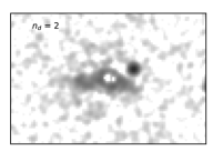
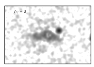
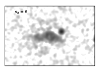
Figure 3: Background-subtracted soft band images of the Spiderweb Galaxy after removing the simulated image of the AGN. The image has been smoothed with a Gaussian kernel with a sigma of 1 pixel, slightly degrading the effective resolution. The normalization of the surface brightness of the diffuse emission within a radius of 2 arcsec is free and it is parametrized with $n_{d}$ ranging from 1 (upper left image) to 6 (lower-right image). There are a few slightly negative pixels in the image, so that the average pixel value far from the Spiderweb Galaxy is zero. The unresolved source close to the center is an AGN that has not been subtracted from the image.

Assuming that the diffuse emission in the hard band is negligible, we focus on the soft band and attempt to reconstruct an image of the Spiderweb Galaxy removing the dominant AGN emission. This can be obtained simply by subtracting the normalized PSF image from the real data. Clearly, the slope of the PSF image on the scale of 1 arcsec is so steep that an uncertainty on the order of 1 pixel on the relative astrometry of the real data and of the ray-tracing simulation does not allow an accurate subtraction, and may result in a distorted distribution of net counts. After the subtraction, in fact, the resulting image shows a small number of pixels with negative values (about ten), all very close to the center. Such negative values can be eliminated with a simple redistribution, consisting in averaging iteratively the maximum and minimum pixel values within the inner 2 arcsec, untill no negative pixels are left (about 10 iterations). This procedure preserves the photometry, but the final distribution of the pixel values is not accurate on the scale of $\sim 1$ arcsec. Finally, we smooth the images with a 2D Gaussian kernel with a size of 1 pixel, to obtain a less noisy image without loss of information, and to subtract the average instrumental plus sky background as estimated from the 16^′′-29.5^′′ annulus.

The background-subtracted, soft-band images of the Spiderweb Galaxy after the removal of the AGN emission are shown in Figure 3 for $n_{d}$ ranging from 1 to 6. As previously mentioned, the presence of a hole in the center for $n_{d}<3$ is an artifact of the method used to reconstruct the image, and reflects our ignorance on the distribution of surface brightness on scales on the order of 1 arcsec in the regions dominated by the AGN emission. As a consequence, we focus only on the global photometry within a radius of 2 arcsec, ignoring anomalies in the surface brightness distribution. The images shown in Figure 3, however, still allow us to appreciate that the choice $n_{d}\geq 4$ corresponds to an almost uniform, prominent core in the innermost 17 kpc, nicely matching the surface brightness level robustly measured outside 2 arcsec (where the effects of a sub-pixel mismatch are much smaller due to the rapidly flattening shape of the Chandra PSF). As previously discussed, the choice $n_{d}=4$ corresponds to a prominent, but still plausible, cool core. Thus, we adopt $n_{d}=4$ as a reference value to estimate the central ICM density, stressing that the exact value has a mild impact on all the conclusions derived in this work.

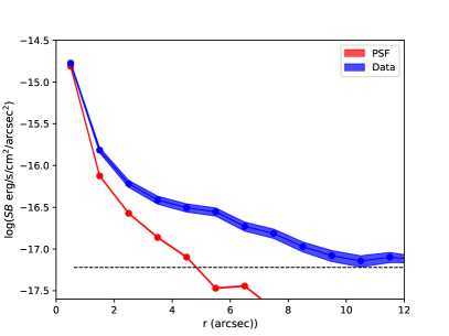
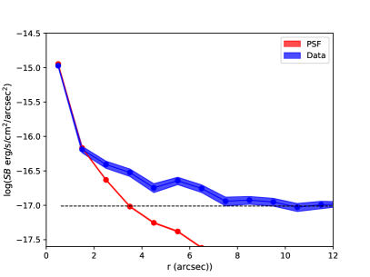
Figure 4: Left: Azymuthally averaged profile of the AGN simulated image (normalized to $n_{d}=4$, red line) compared to the soft-band Spiderweb profile (blue line). The horizontal line shows the instrumental plus unresolved X-ray background level. Right: same in the hard (2-7 keV) band.

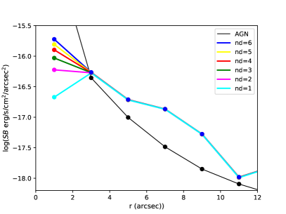
Figure 5: Azymuthally averaged profile of the diffuse emission (after subtraction of the AGN emission and of the background) at different $n_{d}$ values. As expected, only the innermost bin is affected by the choice of $n_{d}$, while the indirect effects on the normalization of the AGN contamination, thus on the overall normalization of the diffuse emission, is negligible. The black line is the simulated AGN emission for comparison.

To further support this choice, we look directly at the surface brightness profile of the simulated AGN and the real data, in both bands. We note that the effect of the normalization of the AGN image corresponding to different values of $n_{d}$ is affecting only the first bin of the profile ($r<1$ arcsec), while all the other bins (at $r>1$ arcsec) are practically unaffected. In the left panel of Figure 4 we show the azymuthally averaged profile of the AGN simulated image (for the specific choice $n_{d}=4$) compared to the Spiderweb profile in the soft band. We notice that the data show signal in excess of the unresolved nuclear source at $r\geq 1.5$ arcsec, while in the hard band (shown in the right panel), the excess starts to appear only at $r\geq 2.5$ arcsec. Since the measurement of the diffuse emission at $r\geq 1.5$ arcsec is practically independent of the $n_{d}$ value, we note that an approximately constant increase of the surface brightness toward the center is obtained for $3<n_{d}<4$. This is shown in Figure 5, where we plot the azymuthally averaged surface brightness profile of the extended emission in the soft band (that is, the difference of the data and the PSF model shown in the left panel of Figure 4). Unfortunately, at the moment we do not have compelling argument to strongly constrain the value of $n_{d}$. The implications of values different from $n_{d}=4$, as adopted in this work, will be investigated in Lepore et al. (in preparation).

From the right panel of Figure 4, we also notice that the hard band emission is less extended than the soft emission, that is detected well above the background up to 12 arcsec ($\sim 100$ kpc) from the nucleus of the Spiderweb Galaxy. Instead, in the hard band there is no excess at $r\leq 2^{\prime\prime}$, and the diffuse emission is less significant and limited to the range $3^{\prime\prime}<r<7^{\prime\prime}$. This suggests that the diffuse emission is contributed by two distinct components. The one with larger hardness ratio is less extended and is most likely associated with the IC from the relativistic population of electrons in the jet. The soft component is more extended up, to a distance of $\sim 100$ kpc from the center, and is possibly associated with hot gas. In the following section we proceed with the spectral analysis of the AGN-dominated emission included within a radius of 17 kpc, while in Section 6 we investigate the diffuse emission at radii $>2^{\prime\prime}$, after accounting for the background and AGN contamination.

5 X-ray properties of the Spiderweb Galaxy: spectral analysis of the central AGN

5.1 Global nuclear emission

Compared to the shallower X-ray observation presented in Carilli et al. (2002), our new, deep exposure allows us to obtain a more detailed spectral analysis of the nuclear emission, and, in particular, to investigate the contribution of the diffuse component, on the basis of the accurate imaging analysis presented in the previous Section. In the following, we perform our reference analysis of spectra extracted separately from each Obsid, and for which we consider the respective Obsid ARF and RMF calibration files. Ultimately, this info are considered all together during the fitting procedure. This approach allows us to keep track of the different effective area corresponding to each Obsid. Eventually, we also analyze the spectrum obtained by merging the single Obsid spectra, using cumulative ARF and RMF files obtained by weighting single Obsid files by the corresponding exposure times. We find that this approach gives results that are in agreement with our reference spectral analysis. Given the brightness of the source, each Obsid has at least 300 net counts within the extraction region (a 2^′′ radius circle). Therefore, we compute the ARF and RMF files for each one of the 22 Obsid.

We fit the nuclear emission with Xspec 12.11.1 (Arnaud, 1996) over the 0.5-9.0 keV energy range, adopting the simplest possible model, as done for the analysis of the protocluster members in Paper I. The AGN emission is, therefore, described by an intrinsically absorbed power law, using the model components zwabs and powerlaw. The galactic absorption is described with the model tbabs, and its value is fixed to $3.18\times$ 10²⁰ cm^-2 according to the HI map of the Milky Way (HI4PI Collaboration et al., 2016).

As previously discussed, the contribution from diffuse emission within 2 arcsec cannot be constrained accurately but it must be parametrized by the enhancement factor $n_{d}$, that represents the ratio of the surface brightness within 2 arcsec over that measured in the 3-5 arcsec annulus. As a preliminary test, we perform a straightforward spectral analysis assuming two background files: the first including only the instrumental plus unresolved background, sampled in the annular region between 16 and 24 arcsec; the second including instrumental background and extended emission contribution directly sampled in the 3-5 arcsec annulus. The last choice corresponds to the assumption that the surface brightness of the diffuse emission is constant within 5 arcsec with no central enhancement ($n_{d}=1$). We find that the fit obtained in the second case significantly improves, with $\Delta C_{stat}\sim 23$. This simply confirms that we must account for some contribution from diffuse emission within 2 arcsec, possibly with $n_{d}>1$, as we already shown from the imaging analysis. At the same time, the best-fit spectral parameters of the AGN emission model are in agreement within 1 $\sigma$ irrespective of the background treatment, confirming that the contribution of the diffuse emission is very low compared to the nuclear emission. This is expected also from photometry, since we measure 9710 net counts in the 0.5-7 keV band within 2 arcsec, while, from the imaging analysis, we expect only $95\times(n_{d}/3)$ and $8\times(n_{d}/3)$ net counts in the soft and hard bands, respectively, from diffuse emission. Overall, within a radius of 2 arcsec, we expect a fraction of $0.015\times(n_{d}/3)$ of the total emission to be not associated with the AGN in the soft band, and only $0.003\times(n_{d}/3)$ in the hard band. Such contribution is so small that $n_{d}$ cannot be constrained by spectral analysis.

As a next step, we search for the best spectral modelization of the diffuse emission, fitting the emission within the 3-5 arcsec annulus after instrumental background subtraction and after accounting for 1.5% of the nuclear emission expected in that region. We find that statistically equivalent fits are obtained with a thermal mekal model or power law, with $kT\sim 3.0$ keV and $\Gamma\sim 2.7$, respectively. On the other hand, the fit considerably gets worse if $\Gamma=2$ is assumed (with $\Delta C_{stat}\sim 16$). This shows us that the diffuse component in this region is better described by a soft, thermal emission than by a nonthermal, $\Gamma\sim 2$ power-law emission. Therefore, we describe the weak diffuse component within 2 arcsec by using a mekal model with $kT=3$ keV.

Incidentally, we note that we do not consider here a nuclear plus diffuse contribution possibly associated with star formation. The total SFR associated with the core of the Spiderweb Galaxy plus the star-forming satellite galaxies (the so-called flies) has been estimated to range from $70M_{\odot}$/yr (Hatch et al., 2009) to $1400M_{\odot}$/yr (Seymour et al., 2012), and is expected to be significantly obscured. If we maximize the star-formation (SF) contribution with an unabsorbed spectrum with $\Gamma\sim 2.0$, we find that in our data we expect $\sim 2.9\times({\rm SFR}/100M_{\odot}/yr)$ net counts in the 0.5-7.0 keV range. Considering the maximum value of $1400M_{\odot}$/yr, we estimate an upper limit of 40 net counts to the SF contribution within 2 arcsec, which is about 0.3% of the AGN component and, therefore, can be safely ignored. The possible contribution from SF associated with the Ly$\alpha$ halo, has been estimated to be in the range $60-140M_{\odot}$/yr, and is also expected to be completely negligible in the annular region between 2^′′ and 12^′′ that we consider in the Section 6.

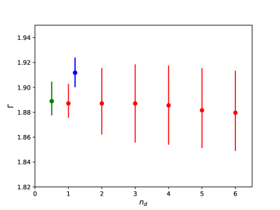
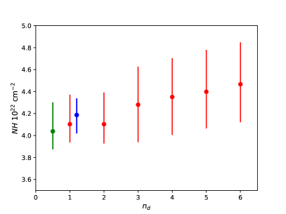
Figure 6: Left: Best-fit spectral slope $\Gamma$ of the nuclear emission of the Spiderweb as a function of the enhancement factor $n_{d}$ (red points). The best-fit values obtained with direct background subtraction are shown as blue and green points, where blue is for the background sampled in the 2.6-4.6 arcsec annulus, and green in the 16-24 arcsec annulus. Right: Same for the best-fit value of the intrinsic absorption $N_{H}$.

Now we focus on the spectral analysis of the nuclear emission. In Figure 6 we show the best fit values as a function of the enhancement factor $n_{d}$ that paramterizes the normalization of the diffuse component within 2 arcsec. We see that the spectral slope $\Gamma$ is hardly affected, since it is robustly constrained by the hard-band signal at energies larger than 2 keV, where the contribution of diffuse emission is estimated to be very small. However, when compared to the values obtained with direct background subtraction, with and without the inclusion of the foreground as estimated in the 3-5 arcsec annulus, we find that the 1 $\sigma$ uncertainties almost double, even though it is still below 2%. This marginal but noticeable effect is simply due to the fact that the inclusion of a small thermal contribution makes the model more similar to the data, resulting in a milder dependence of $C_{stat}$ on the parameters of the fit, hence larger error bars. We also note that the inclusion of a thermal component with a fixed $n_{d}$ does not imply additional free parameters (in other words, not only the normalization but also the shape, namely temperature and metallicity, are kept frozen). When we turn to the intrinsic absorption $N_{H}$ (right panel of Figure 6), we notice that the best fit value increases slightly with $n_{d}$. We do expect this trend since, when the thermal component increases, the nuclear emission in the soft band is correspondingly reduced, and this is compensated with a slightly larger intrinsic absorption. Here the typical 1 $\sigma$ error bar is constant at the level of 5%. As expected, these results do not change if we describe the diffuse emission with a $\Gamma\sim 2.7$ power law instead of a $\sim 3$ keV mekal model. To summarize, the investigation of the effect of the diffuse emission within a radius of 2 arcsec on the spectral analysis of the nuclear emission, shows that the properties of the nuclear emission are marginally affected by the parameter $n_{d}$. According to the discussion in Section 4.2 based on our imaging analysis, in the following we assume a value $n_{d}=4$ for reference, bearing in mind that different $n_{d}$ values would not impact the results presented in this work.

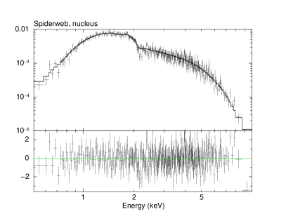
Figure 7: Merged spectrum (folded with the instrument spectral response) of the nucleus of the Spiderweb Galaxy with the best fit model (first column of Table 1, with $n_{d}=4$). The residuals are shown in the bottom panel. There is no significant excess in the soft band, showing that diffuse emission is properly accounted for within the limits of the spectrum quality.

Table 1: Best-fit values for the reference spectral analysis of the nuclear emission of the Spiderweb Galaxy assuming $n_{d}=4$. Fluxes are corrected for Galactic absorption, while luminosities are corrected both for Galactic and intrinsic absorption

.

parameter	aperture (2′′)	PSF correction
$\Gamma$	$1.883_{-0.012}^{+0.016}$	$1.85\pm 0.02$
$N_{H}$	$4.23_{-0.17}^{+0.28}\times 10^{22}$	$4.2_{-0.2}^{+0.3}\times 10^{22}$
$F_{S}$	$5.64\pm 0.17\times 10^{-14}$	$5.95\pm 0.18\times 10^{-14}$
$F_{H}$	$1.38\pm 0.02\times 10^{-13}$	$1.51\pm 0.02\times 10^{-13}$
$L_{0.5-2keV}$	$3.10\pm 0.09\times 10^{45}$	$3.27\pm 0.10\times 10^{45}$
$L_{2-10keV}$	$4.29\pm 0.05\times 10^{45}$	$4.68\pm 0.05\times 10^{45}$

We also consider aperture correction that introduces a mild spectral distortion due to the different PSF in the soft and hard bands. From the AGN ray-tracing simulations, we estimate that total soft and hard fluxes and luminosities are larger by a factor $1.05$ and $1.09$, respectively, compared to that measured within 2 arcsec. Fluxes are corrected only for the Galactic absorption, while luminosities are corrected for both Galactic and intrinsic absorption. Error on fluxes and luminosities account for the uncertainty associated with the full range $n_{d}=1-6$ and are 3% in the soft and 1% in the hard band. The effect of the PSF correction on the spectral shape is instead very mild, with the intrinsic slope $\Gamma$ being harder by less than 2%. We verified a posteriori that the fit is not sensitive to the assumed value for the parameter $N_{HGal}$ that describes the Galactic absorption. If left free, $N_{HGal}$ has a best-fit value of $3.2_{-0.9}^{+1.6}\times 10^{20}$ cm^-2, right on top of the value based on the HI map of the Milky Way (HI4PI Collaboration et al., 2016). Finally, we search for the presence of a neutral iron line at 6.4 keV rest-frame, corresponding to 2.03 keV in the observing frame, but we found no signal. The mild obscuration corresponds to a source dominated by the transmitted emission, while significant iron line are expected when the reflected component is dominant. If we perform a blind search for emission lines in the range 1-7 keV, we do not find any significant candidate. The merged spectrum and the best-fit model, along with the residuals, are shown in Figure 7. The residuals are very regular with no significant departure from pure noise. In particular, we do not find significant residuals in the soft band, showing that the diffuse emission is properly accounted for within the limits of the spectrum quality. Our best-fit model for the nuclear spectrum of the Spiderweb Galaxy is shown in Table 1, with and without aperture correction in terms of normalization and spectral shape.

In conclusion, an X-ray obscuration at the level of $4.2\times 10^{22}$ cm^-2 can be provided by the surrounding galactic medium and circumgalactic medium as observed in high-z galaxies in the CDFS (Circosta et al., 2019; D’Amato et al., 2020a), or in the BCG of a $z\sim 1.7$ protocluster (D’Amato et al., 2020b). Therefore it is plausible that the obscuration is not dominated by a torus, and that the AGN in the Spiderweb Galaxy is an unabsorbed, TypeI quasar, as also suggested by the detection of broad lines. This would be unusual since radio galaxies are typically associated with obscured TypeII AGN. However, the peculiar phase of the Spiderweb Galaxy may justify the copresence of a strong quasar and a strong radio activity.

5.2 Spectral variability

We can investigate the variability of the AGN in the Spiderweb Galaxy on a scale of $\sim 9$ months, which is the time span over which the observations of the Large Program have been taken (November 2019 - August 2020). In addition, we have one measurement at a distance of $\sim 20$ years (in 2000), and the timescale provided by the single Obsid duration, from a minimum of 5 to a maximum of 14 hours.

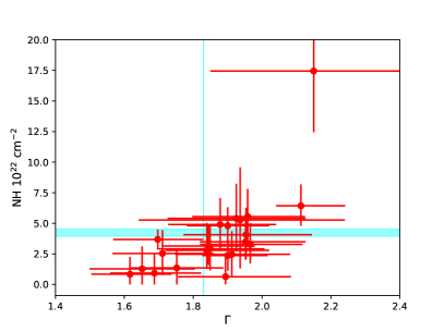
Figure 8: Scatter plot of the best fit values of the intrinsic absorption $N_{H}$ and the spectral slope $\Gamma$ for each Obsid. Error bars refer to 1 $\sigma$ c.l. on a single parameter. Shaded area show the 1 $\sigma$ interval for the best fit value of $N_{H}$ from the global fit.

First we investigate the spectral variability. We fit separately each Obsid and we plot the distribution of best fit values for $N_{H}$ and $\Gamma$. We note that for the fits of each Obsid we do not apply the small PSF correction to the spectral shape. As we show in Figure 8, the distribution of the best-fit values in the $N_{H}$-$\Gamma$ plane appears to be roughly consistent with the global best-fit, with the apparent correlation due to the well-known degeneracy of $N_{H}$ and $\Gamma$. If we compute a simple reduced $\chi^{2}$ with respect to the average value (after removing the unique outlier with $N_{H}>10^{23}$ cm^-2 obtained for Obsid=22922), we find $\chi^{2}\sim 0.98$ and $\chi^{2}\sim 1.21$ for 21 degrees of freedom, for $\Gamma$ and $N_{H}$, respectively. In both cases we are not able to reject the null hypothesis of a constant value also in the case of $N_{H}$, for which we have a probability slightly less than $0.25$ to obtain a larger $\chi^{2}$. If we do not remove the unique strong outlier (corresponding to Obsid=22922), we are able to reject the null hypothesis of a constant $N_{H}$ on the entire observing period with a probability less than $0.05$ to obtain a larger $\chi^{2}$. To summarize, from a simple $\chi^{2}$ test on the entire data set, we get only a weak hint, if any, of spectral variability.

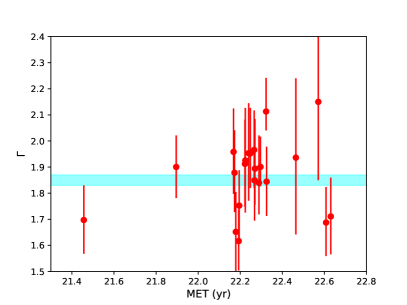
Figure 9: Best-fit values of $\Gamma$ for each Obsid as a function of the Mission Timeline $MET$ (years). The first point has been moved to $MET=21.5$ to be shown in the same linear plot. The horizontal shaded line shows the best-fit value of the cumulative spectrum with PSF correction, as listed in Table 1.

Then, in Figure 9 and 10 we plot the best-fit values of $\Gamma$ and $N_{H}$ as a function of the Mission Timeline (MET). In Figure 9 we can see that $\Gamma$ is consistent with the best-fit value of the spectral analysis of the cumulative spectrum for each Obsid within 1 $\sigma$, as confirmed by a simple $\chi^{2}$ test. On the other hand, in Figure 10 we find that $N_{H}$ shows a higher level of fluctuations, and that the lowest values of $N_{H}$ seems to occur in contiguous periods within a narrow time frame. We repeat the plot after freezing the spectral slope to the average best-fit value $\Gamma=1.88$. This reduces the noise around the average value, removing the degeneracy between $N_{H}$ and $\Gamma$, but the period with low $N_{H}$ is still visible (see Figure 10, lower panel). Actually, when $\Gamma$ is frozen, the reduced $\chi^{2}$ with respect to a constant $N_{H}$ value increases to $\chi^{2}=1.65$ despite the smaller scatter, due to the smaller error bars, after the removal of the single outlier (Obsid 22922). To quantify the spectral variability of $N_{H}$ we discard the outlier and focus on three contiguous periods. One is when a low $N_{H}$ is measured, corresponding to $22.179<{\rm MET}<22.323$, while the rest consists in all the observations before ${\rm MET}=22.179$ and after ${\rm MET}=22.323$. We obtain $N_{Hhigh}=(5.02\pm 0.32)\times 10^{22}$ cm^-2 and $N_{Hlow}=(2.95\pm 0.24)\times 10^{22}$ cm^-2, with a difference of a factor $\sim 1.7$ of $\sim 5$ $\sigma$. To summarize, we conclude that we see a modest but significant spectral variation corresponding to a change in the intrinsic absorption by a factor $\sim 1.7$ on a timescale of $\sim 1$ year. This also implies that part of the intrinsic absorption happens close to the SMBH and it is associated with a clumpy obscuring torus, while part of the absorption may still be associated with the intergalactic medium, as suggested in Section 5.1.

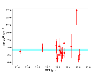
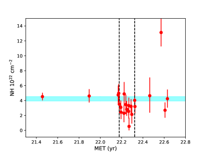
Figure 10: Upper panel: Best-fit values of $N_{H}$ for each Obsid as a function of the Mission Timeline $MET$ (years). The first point has been moved to 21.5 to be shown in the same linear plot. The horizontal shaded line shows the best-fit value of the cumulative spectrum with PSF correction, as listed in Table 1. Lower panel: Same, but with best-fit values of $N_{H}$ obtained with $\Gamma$ frozen to 1.88. The vertical dashed lines bracket the period with low intrinsic absorption as discussed in the text.

5.3 Flux variability

We compute the soft and hard band flux values in each Obsid keeping $\Gamma=1.88$ frozen, and correcting for the Galactic absorption. The result is shown in Figure 11. We note that for simplicity here we report the fluxes within 2 arcsec, without correcting for the PSF effects in each band, since our discussion would not be affected by this correction. We notice a significant variability on a scale of a few months in the observing frame. If we fit the flux as a function of the time with a constant, the reduced $\chi^{2}$ is $\sim 3.0$ in both bands for 21 degrees of freedom (for consistency, we conservatively removed Obsid 22922 that appears to be an outlier both for shape and normalization of the spectrum). Also if we remove the lowest and highest points, we still obtain a reduced $\chi^{2}\sim 2$ with 19 degrees of freedom. The rms fluctuation is $12$% in both bands, therefore very mild, however it is statistically significant. In addition, we note that the flux variability seems to have a temporal behavior different from the spectral variation (or change in $N_{H}$). This can be seen by the lack of correlation between the best-fit $N_{H}$ values and the percentage variation of the flux, shown in Figure 12. Therefore, we conclude that we are able to detect variability both in the normalization of the spectrum and in the spectral shape, and that there are no signs of correlation between the two phenomena.

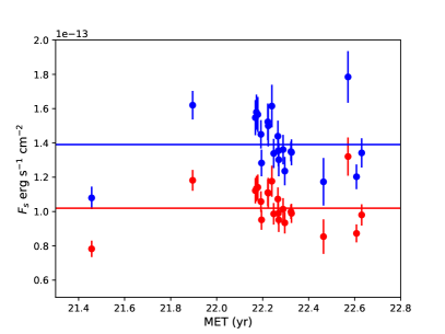
Figure 11: Soft (red points) and hard (blue points) flux values measured in each Obsid within a radius of 2 arcsec as a function of the Mission Timeline. Fluxes are corrected for the Galactic absorption. Horizontal lines show the average values.

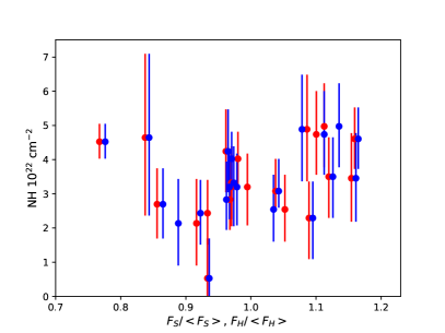
Figure 12: Best-fit values of $N_{H}$ plotted against the ratio of the flux in each Obsid over the average flux (red and blue dots correspond to the soft and hard bands, respectively).

6 X-ray properties of the Spiderweb Galaxy: Diffuse emission

6.1 Imaging analysis

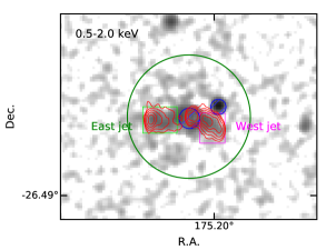
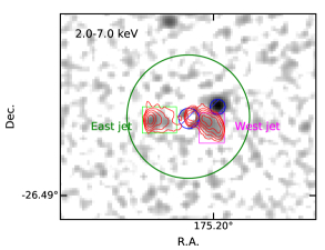
Figure 13: Left: Background-subtracted soft band image of the Spiderweb Galaxy after AGN subtraction (with $n_{d}=4$). The image has been smoothed with a Gaussian kernel with a sigma of 1 pixel, slightly degrading the effective resolution. The green and magenta boxes correspond to the regions used for the east and west jet spectral analysis, respectively. Two AGN circular extraction regions (in blue) are removed (the AGN, with a radius of 2 arcsec, and a nearby AGN with a radius of 1.5 arcsec). The large green circle is the region used for the spectral analysis of the isotropic diffuse emission, excluding both jet regions and the AGNs. Red contours show radio emission observed in the 10 GHz band with the JVLA (Carilli et al., 2022) at levels of $0.03$, $0.2$, $2$ and $20$ mJy/beam.

In Figure 13 we show the extraction regions used for our analysis of the diffuse emission, overplotted on the background-subtracted images after removing the central AGN (we used $n_{d}=4$ for display). Consistently with the radio and X-ray combined analysis of the jets presented in Carilli et al. (2022) and Anderson et al. (2022), we select two box regions for the east and west jet regions. These regions cover all the radio emission observed at 10 GHz (see Carilli et al., 2022), include most of the diffuse emission in the soft band (see Figure 13, left) and almost the entire diffuse emission in the hard band (see Figure 13, right). The extraction region for the analysis of the diffuse emission outside the jet region is obtained by selecting a circle centered on the Spiderweb Galaxy with a radius of 12 arcsec, corresponding to $\sim 100$ physical kpc at $z=2.156$. From this circular region, we remove two boxes corresponding to the east and west jets, and two circular regions corresponding to the central AGN (a circle with a radius of 2 arcsec) and to the source XID 7 (a circle with a radius of 1.5 arcsec) that is found to be a companion quasar (see Paper I). The boxy shape is chosen to follow at best the jet shape and to keep, at the same time, a simple geometry. The instrumental plus unresolved extragalactic X-ray background is sampled from an annulus with inner and outer radius of 16 and 29.5 arcsec, respectively, which is the same used for the analysis of the nuclear emission.

In Figure 13, it is possible to appreciate that the diffuse emission in the soft band is clearly visible outside both jet regions, out to a radius of 12^′′ from the nucleus, while the shape of the diffuse emission in the hard band is almost entirely elongated along the radio jets, with no emission elsewhere. On the basis of this preliminary imaging analysis, we argue that the emission along the jets is dominated by IC emission from the relativistic jet population, while the more isotropic soft emission may be dominated by thermal emission from shocked gas. The diffuse emission along the jets is clearly harder, as expected in case of a power law, nonthermal emission, while the diffuse emission outside the jet regions has an hardness ratio $HR\sim-1$, being entirely soft, as expected in the case of thermal emission with a relatively low temperature, or a very steep power law. Incidentally, this result may provide another piece of evidence that inverse Compton losses are important in high-z radio sources, and that this effect is likely to be a strong contributor to the well-known correlation between ultra-steep spectrum and redshift for radio sources (Tielens et al., 1979; Blumenthal & Miley, 1979; Morabito & Harwood, 2018). On the other hand, another plausible mechanism for a steep radio spectrum may be associated with an increased ambient density (Klamer et al., 2006). Clearly, both mechanisms may be at play in the Spiderweb Galaxy. A systematic exploration of high-z radio galaxies in a variety of environments would be key to understand the physics behind the correlation between redshift and their spectral properties. This relevant aspect is not explored in this work, but it constitutes a clear science case for future Chandra programs.

While the nature of the diffuse emission is further investigated in our spectral analysis, as a preliminary step, we obtain the photometry in the three different regions. We find $207\pm 19$ and $228\pm 21$ net counts in the 0.5-7 keV band in the west and east jet regions, respectively, after subtracting the background. In the circular region with a radius of 12 arcsec, after removing the west jets, east jet, and AGN regions, we measure $447\pm 53$ net counts in the 0.5-7 keV band. We note that the isotropic, diffuse component, where we expect to find thermal emission, overlaps with the west and east jet regions, while the AGN wings overlaps with all the diffuse components. Therefore, we have to take into account two and three components to perform spectral analysis of the isotropic diffuse emission and the jet emission, respectively. While we already have established the shape and normalization of the AGN emission, we need to measure first the diffuse, isotropic emission (accounting for AGN contamination), and finally the emission in the two jet regions (accounting for AGN contamination and isotropic emission).

Table 2: Best-fit values for the reference spectral analysis of the diffuse emission. We note that in this table, flux and luminosity values of the isotropic (thermal) emission have not been corrected by the geometrical factor, but directly correspond to the best-fit values obtained from the extraction region. Error bars refer to 1 $\sigma$ c.l. on a single parameter.

region	$kT$ (mekal)	$F_{S}$	$F_{H}$	$L_{0.5-2keV}$	$L_{2-10keV}$
	keV	erg s-1 cm-2	erg s-1 cm-2	erg s-1	erg s-1
isotropic	$1.98_{-0.43}^{+0.70}$	$(2.5\pm 0.6)\times 10^{-15}$	$(2.4\pm 0.9)\times 10^{-16}$	$(7.7\pm 1.8)\times 10^{43}$	$(7.3\pm 1.7)\times 10^{43}$
region	$\Gamma$	$F_{S}$	$F_{H}$	$L_{0.5-2keV}$	$L_{2-10keV}$
	-	erg s-1 cm-2	erg s-1 cm-2	erg s-1	erg s-1
west jet	$1.90\pm 0.20$	$(1.32\pm 0.21)\times 10^{-15}$	$(1.78\pm 0.28)\times 10^{-15}$	$(4.1\pm 0.7)\times 10^{43}$	$(5.5\pm 0.9)\times 10^{43}$
east jet	$2.51\pm 0.21$	$(1.89\pm 0.25)\times 10^{-15}$	$(1.02\pm 0.13)\times 10^{-15}$	$(1.18\pm 0.15)\times 10^{44}$	$(6.4\pm 0.8)\times 10^{43}$

6.2 Spectral analysis of the diffuse emission: Isotropic component

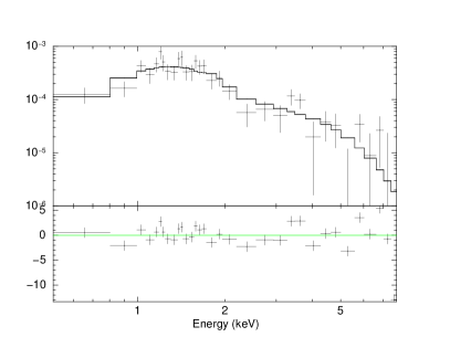
Figure 14: Left: Spectrum (folded with the instrument spectral response) of the isotropic diffuse emission (after removing the central, AGN-dominated region, and the jet regions) fitted with a thermal mekal model plus the AGN contamination. Right: Unfolded spectrum with the two model components shown with dotted lines. The AGN contamination (absorbed power law) is dominant at energies $>1.5$ keV, while the thermal component is dominant below $1$ keV.

The spectral fits are performed with Xspec 12.11.1 (Arnaud, 1996) over the energy range 0.5–9.0 keV of the merged spectrum. In fact, we do not use single Obsid for the fits, since several observations would have less than 10 net counts, so that the spectral shape is completely undetermined in each separate Obsid. In this case, we use cumulative ARF and RMF files obtained by weighting single Obsid files by the corresponding exposure times. Galactic absorption is described with the model tbabs and its value is fixed to $3.18\times 10^{20}$ cm^-2. We used Cash statistics (Cash, 1979) applied to the source plus background, which is preferable for low S/N spectra (Nousek & Shue, 1989). We assume that the emission observed within 12 arcsec is approximately symmetric and centered on the Spiderweb Galaxy. We fit the diffuse emission outside the jet regions, after removing the AGN as previously described, with a mekal model and a power law model.

From the ray-tracing simulation, we find that $3.3$% of the soft nuclear emission inside 2 arcsec is found in the extraction region. Therefore, we add this component modeling it with an absorbed power law with the parameters frozen to the best-fit values found in the AGN extraction region, including the correction for the PSF effect that makes the AGN contamination slightly harder than the spectrum measured within 2 arcsec. This last correction implies that $\Gamma=1.85$ is a suitable expectation. We also do not include the neutral iron line component, since it has been found to be negligible (see Section 5.1). The Galactic absorption is clearly the same for both components. Therefore, after accounting for a fixed component associated with the AGN contamination, we perform a fit of the isotropic diffuse emission, that, as thoroughly discussed in the imaging analysis (Section 4.2) is almost entirely included in the soft band.

The unabsorbed power law model has a best-fit slope of $\Gamma=3.27\pm 0.43$ for a flux of $(2.7\pm 0.7)\times 10^{-15}$ erg s^-1 cm^-2 and $(4.9\pm 2.6)\times 10^{-16}$ erg s^-1 cm^-2 in the 0.5–2 keV and 2–10 keV bands. If, instead, we assume a thermal model, we find that the fit improves with a $\Delta C\sim 10$. We obtain a best-fit temperature of $1.98_{-0.43}^{+0.70}$ keV and metallicity of $Z=0.26_{-0.26}^{+1.35}Z_{\odot}$, or better, a $1\sigma$ upper limit $Z<1.6Z_{\odot}$. . We remark that the 1 $\sigma$ error bars (or upper limits) are obtained by varying a single parameter, keeping the other parameters frozen to their best-fit values. The measured fluxes are $(2.5\pm 0.6)\times 10^{-15}$ erg s^-1 cm^-2 and $(2.4\pm 0.9)\times 10^{-16}$ erg s^-1 cm^-2 in the 0.5–2 keV and 2–10 keV bands, consistent with those found for the power law model. The 0.5-10 keV rest-frame luminosity is $L_{0.5-10{\tt keV}}=(1.50\pm 0.36)\times 10^{44}$ erg s^-1. To correct for the excluded area (the jet regions and the AGN extraction region), we can assume an approximately constant surface brightness and apply a geometric correction factor of 1.22, obtaining $L_{0.5-10{\tt keV}}=(1.83\pm 0.44)\times(1+0.03\,n_{d})\times 10^{44}$ erg s^-1, that, for our reference choice $n_{d}=4$, is equal to $L_{0.5-10{\tt keV}}=(2.0\pm 0.5)\times 10^{44}$ erg s^-1. A more accurate study including a detailed analysis of the surface brightness distribution will be presented in a forthcoming paper (Lepore et al., in preparation).

The spectrum fitted with a thermal component is shown in Figure 14. In the right panel we show that the AGN contamination is dominant at energies $>1.5$ keV, while the thermal component is higher below 1 keV. We find that the AGN contamination contributes 25% and 92% of the signal in the soft and hard bands, respectively. From a statistical point of view, the thermal model is marginally better than a power law model ($\Delta C\sim 10$ with an additional degree of freedom). However, the slope of the power law model is softer than the AGN emission at 3$\sigma$ c.l. This implies that the diffuse emission cannot be simply ascribed to contamination from the AGN, and that it is unusually steep for nonthermal emission mechanisms. Therefore, adding these aspects to the statistical improvement obtained with the thermal model, we conclude that the diffuse almost isotropic emission detected within 12 arcsec around the Spiderweb Galaxy is very likely due to thermal emission from diffuse hot baryons. Unfortunately, as already mentioned, we cannot detect the emission line complex of the H-like and He-like iron ions because of the low S/N and for the unfortunate rest-frame position of the iron lines at $\sim 2.1-2.2$ keV. Moreover, the large K-correction combined with the loss of sensitivity below 1 keV, makes it unfeasible to use the iron L-shell complex to efficiently constrain metallicity and temperature. However, the formal best-fit value for the metallicity $Z=0.26_{-0.26}^{1.35}\,Z_{\odot}$ leaves room for enrichment above solar abundance. Finally, we would like to point out that the presence of ICM is strongly corroborated by the successful detection of SZ signal in the same position and shape of the X-ray diffuse emission, providing a completely independent and remarkably consistent measurement of the ICM (Di Mascolo et al., in preparation).

A final note on the ICM temperature: we notice that the best fit value of $1.98_{-0.43}^{+0.70}$ keV is somewhat lower than the $\sim 3$ keV component we assumed to account for the diffuse emission within a radius of 2 arcsec when fitting the AGN spectrum. In fact, one may expect the opposite, if any, with a lower temperature associated with denser, central ICM as in normal cool core. However, we must bear in mind that, apart from the unavoidable large uncertainties on its spectral shape, the diffuse component overlapping the outshining AGN emission is necessarily a mix of thermal emission associated to the central ICM and nonthermal emission associated with the bases of the jets, and therefore it is actually expected to be harder. Needless to say, it is impossible to speculate about the share of thermal and nonthermal emission within a distance of 2 arcsec ($\sim 17$ physical kpc).

If we consider the best estimate for an evolved L-T relation, for a temperature of 2 keV, we obtain $L_{X}=1.0\times 10^{44}$ erg s^-1 and $L_{X}=0.7\times 10^{44}$ from Reichert et al. (2011) and Pratt et al. (2009), respectively, where $L_{X}$ is the bolometric X-ray luminosity. In both cases we applied the phenomenologically estimated evolution correction $E(z)^{-0.23}$ at $z=2.156$. Therefore, our estimate of $L_{0.5-10{\tt keV}}=(2.0\pm 0.5)\times 10^{44}$ erg s^-1 (after including the geometrical correction and the core emission with $n_{d}=4$) is about a factor of 2 above the expected average relation, but still in agreement with it given the large intrinsic scatter observed particularly at low temperatures. This result, if coupled to the forthcoming results from the SZ data, is consistent with the observation of a virialized halo, as we further discuss in Section 7.

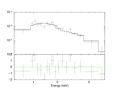
Figure 15: Left: Spectrum (folded with the instrument spectral response) of the emission in the west jet region (including the AGN contamination and the residual thermal emission from the ICM) fitted with a power law. Right: Unfolded spectrum with the three components in the model shown with dotted lines. The lowest dotted line corresponds to the thermal emission from the overlapping ICM, while the line in the middle accounts for the AGN wings contamination. The IC from the relativistic population in the west jet is shown by the unabsorbed power law that is dominating at any energy.

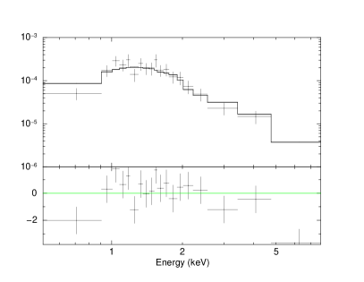
Figure 16: Left: Spectrum (folded with the instrument spectral response) of the emission in the east jet region (including the AGN contamination and the residual thermal emission from the ICM) fitted with a power law. Right: Unfolded spectrum with the three components in the model shown with dotted lines. The lowest dotted line corresponds to the thermal emission from the overlapping ICM, while the line in the middle accounts for the AGN wings contamination. The IC from the relativistic population in the east jet is shown by the unabsorbed power law that is dominating at any energy.

6.3 Spectral analysis of the diffuse emission: Jet regions

To fit the diffuse component in the west and east jet regions, we use a power law emission as a baseline model, being more appropriated for IC emission, as expected along radio jets. On the other hand, we do not include any intrinsic absorption, but only the Galactic absorption. As for the AGN contamination, we apply the same procedure described in Section 6.2. In this case, however, we also need to include the presence of the thermal diffuse emission that is expected to be present also in the jet regions. The uncertainty associated with the thermal component within the two box regions is, however, quite large, since the surface brightness distribution is not known and it may be affected by the jet itself. Therefore, we vary the contribution from the thermal component when constraining the nonthermal emission in the jet regions to explore its effect on the best-fit parameters.

First we focus on the west jet region, which is a rectangle of $4.9\times 5.8$ arcsec² centered on RA=11:40:48.03,DEC=-26:29:10.89. The AGN contamination is obtained by rescaling the emission measured within 2 arcsec by the factor $4.38\times 10^{-3}$. The diffuse thermal component in this region is obtained rescaling the emission measured in the diffuse extraction region by a factor of $7.7\times 10^{-2}$, which corresponds to assuming a constant surface brightness. The best-fit value for the slope of the IC emission is $\Gamma_{west}=1.90\pm 0.20$. We investigate how the slope of the emission depends on our subtraction of the thermal component that we expect in that region. We find that the best-fit $\Gamma$ becomes slightly softer when reducing the normalization of the thermal component, up to a value of $\Gamma=2.00\pm 0.20$ when the thermal component is ignored. The stability of the fit is not surprising, since in this region the fit is driven by the prominent emission in the hard band, and therefore is modestly affected by the uncertainty in the soft band. If we attempt to fit the emission with a thermal model, we obtain an unrealistic temperature of $9.3_{-2.5}^{+3.7}$ keV, and the quality of the fit decreases with $\Delta C_{stat}\sim 9$.

We find fluxes of $(1.32\pm 0.21)\times 10^{-15}$ erg s^-1 cm^-2 and $(1.78\pm 0.28)\times 10^{-15}$ erg s^-1 cm^-2 in the 0.5-2 and 2-10 keV bands, respectively, after correcting for Galactic absorption. These values correspond to luminosities of $(4.1\pm 0.7)\times 10^{43}$ erg s^-1 and $(5.5\pm 0.9)\times 10^{43}$ erg s^-1 in the 0.5-2 and 2-10 keV rest-frame bands, respectively. The spectrum in the west jet region folded with the spectral response, and unfolded, including the three components used for the fit, is shown in Figure 15. We note that the IC emission is more than 3 times larger than the AGN contamination across the entire energy range, while the thermal component is almost negligible.

We then focus on the east jet region, which is a rectangle of $7.0\times 5.1$ arcsec² centered on RA=11:40:48.76, DEC=-26:29:09.29. The AGN contamination is obtained by rescaling the emission measured within 2 arcsec by the factor $5.79\times 10^{-3}$. The diffuse thermal component in this region is obtained rescaling the emission measured in the diffuse extraction region by a factor of $9.2\times 10^{-2}$, which corresponds again to a constant surface brightness. The best-fit value for the slope of the IC emission is $\Gamma_{east}=2.51\pm 0.21$. As in the previous case, we investigate how the slope of the emission depends on the thermal component that we expect in that region. We find that the best-fit $\Gamma$ becomes slowly softer when reducing the normalization of the thermal component, up to a value of $\Gamma=2.57\pm 0.22$ when the thermal component is ignored. If we attempt to fit the emission with a thermal model, instead, we obtain a temperature of $4.2_{-0.7}^{+1.0}$ keV, and the quality of the fit significantly decreases with $\Delta C_{stat}\sim 20$. Therefore, we conclude that also in this regions the emission associated with the east jet is not consistent with being thermal, despite it appears to be significantly softer than the emission found in the west jet region. We thus conclude that also in the east jet region the diffuse emission is dominated by nonthermal processes associated with IC from the relativistic electrons. In this regions we find fluxes of $(1.89\pm 0.25)\times 10^{-15}$ erg s^-1 cm^-2 and $(1.02\pm 0.13)\times 10^{-15}$ erg s^-1 cm^-2 in the 0.5-2 and 2-10 keV bands, respectively. We find luminosity of $(1.18\pm 0.15)\times 10^{44}$ erg s^-1 and $(6.4\pm 0.8)\times 10^{43}$ ergs s^-1 cm^-2 in the 0.5–2 and 2–10 keV rest-frame bands, respectively. The folded and unfolded spectra in the east jet region, including the three components used for the fit, are shown in Fig. 16.

On a more quantitative ground, the difference in spectral slope with respect to the west jet region is $\Delta\Gamma=0.61\pm 0.29$, and therefore is significant at 2$\sigma$ c.l. This difference can be interpreted in two ways. The first possible explanation is the presence of an additional thermal component associated with some gas shocked by the east jet itself up to temperatures of few keV. However, this would imply an amount of hot gas at least comparable if not larger than that expected from the ICM within the east jet box, which seems unlikely. A second explanation can be provided by the presence of an older population of relativistic electrons. In fact, this is the scenario that is discussed in much greater details in Carilli et al. (2022) and Anderson et al. (2022) where the synergy between the Chandra X-ray data and the JVLA radio data is fully exploited.

7 Nature of the isotropic diffuse emission and protocluster dynamical state

As a first-cut analysis of the diffuse isotropic emission, we can consider a flat ICM distribution at least in the core region. This drastically simplified picture is consistent with a beta profile (Cavaliere & Fusco-Femiano, 1978) with a large $\sim 100$ kpc core, and reflects our ignorance of the actual ICM distribution. On the other hand, since the X-ray emission depends on the square of the electron density, a homogeneous gas distribution would rather provide an upper limit to the true ICM mass. Nevertheless, since we focus only on the innermost 100 kpc, the impact of the radial dependence of the ICM density is expected to be modest, and we expect an upper limit close to the actual mass value within the inner 12 arcsec. A more accurate treatment of the distribution of the ICM, including the mild decrease of the surface brightness with radius, and a possible asymmetry, will be presented in a forthcoming paper (Lepore et al. in preparation).

Therefore, by assuming a constant gas density within to 12 arcsec, from the spectrum of the diffuse thermal emission we measure an average electron density of $n_{e}=(1.44\pm 0.23)\times 10^{-2}$ cm^-3, for a total ICM mass of $M_{ICM}\leq(1.67\pm 0.25)\times 10^{12}M_{\odot}$ within a radius of physical 100 kpc. However, this value does not include the emission from the excised jet regions, plus the central 2 arcsec circle. As we already discussed, we treated this aspect assuming a simple geometrical correction applied to the surface brightness, corresponding to a factor of 1.22. Since the electron density is proportional to the square root of the emission, this corresponds to a factor of $\sim 1.10$ for the density. Therefore, the geometrically corrected values are $n_{e}=(1.58\pm 0.24)\times 10^{-2}$ cm^-3 and $M_{ICM}\leq(1.84\pm 0.30)\times 10^{12}M_{\odot}$. A more conservative value would be a simple mean with the addition of a systematic uncertainty bracketing the cases of no correction (corresponding to ICM-empty jet regions) and geometrical correction (ICM-filled jet regions): $n_{e}=(1.51\pm 0.24\pm 0.14)\times 10^{-2}$ cm^-3 and $M_{ICM}\leq(1.76\pm 0.30\pm 0.17)\times 10^{12}M_{\odot}$. The error bars here corresponds to the statistical errors on the normalization, and to the systematics associated with the geometrical correction.

If we blindly apply the hydrostatic equilibrium relation of Vikhlinin et al. (2006, see their Equation 7) for a temperature of $kT=1.98^{+0.7}_{-0.4}$ keV out to 100 kpc (physical), we find a mass of $M(<100\,{\tt kpc})=(1.5^{+0.5}_{-0.3})\times 10^{13}\,M_{\odot}$ by assuming a roughly isothermal distribution (consistent with a total density decreasing approximately as $r^{-2}$ beyond 100 kpc and, therefore, a linearly increasing total mass). The implied upper limit to the ICM mass fraction over the total mass is, therefore, $f_{ICM}\leq(0.12\pm 0.04)$. Incidentally, this value is somewhat higher, and only marginal compatible, with the baryonic fraction measured at the group scale (Eckert et al., 2021), possibly indicating that mechanical feedback has not yet depleted the ICM reservoir in the core. However, this is only a preliminary hint that must be verified after a more careful modelization of the actual ICM distribution.

Applying instead the self-similar mass-temperature scaling relation at a redshift of $z=2.156$ (therefore, assuming that $M_{500}\propto T^{\alpha}E(z)^{-1}$ with $\alpha\sim 3/2$) calibrated on data, we find $M_{500}=(3.0\pm 1.1)\times 10^{13}\,M_{\odot}$ within a radius $r_{500}=(220\pm 30)$ kpc (see also Ettori et al., 2004, that provides consistent results). The hydrostatic-equilibrium mass value linearly extrapolated to $r_{500}$ provides $M(<220\,{\tt kpc})=(3.2^{+1.1}_{-0.6})\times 10^{13}\,M_{\odot}$, in agreement with the scaling relation. We find consistent results also when scaling self-similarly with redshift the $M-T$ relation observed in local groups by Lovisari et al. (2015), obtaining $M_{500}=(2.7\pm 1.3)\times 10^{13}M_{\odot}$. We note that the agreement toward a value $M_{500}=3.0\times 10^{13}M_{\odot}$ essentially relies on the assumption of self similar scaling with redshift, which is approximately tested only up to $z\sim 1$. If the dependence of $M_{500}$ on redshift at a given temperature is significantly milder than the self-similar behavior $M_{500}\propto(1+z)^{-3/2}$ for $z>1$, the extrapolated mass of the halo can be more than a factor of two larger (see, e.g., Bulbul et al., 2019).

To interpret our findings we rely on the cosmological hydrodynamic simulations used to predict the properties of proto-cluster regions at $z\sim 2$ (Saro et al., 2009). These simulations show evidences of ongoing assembly of a dominating central galaxy, with a pattern remarkably similar to that observed for the Spiderweb complex. Saro et al. (2009) also find that the projected galaxy velocity dispersion, the observed level of star formation and the stellar mass of the dominant galaxy suggest that this region should trace the progenitor of a rich cluster, whose mass by $z=0$ would be $\simeq 10^{15}\,M_{\odot}$. It is found that such a structure at $z\sim 2$ should already contain a diffuse X-ray emitting atmosphere of hot gas in hydrostatic equilibrium, which is chemically enriched at a level comparable to that of nearby galaxy clusters. To compare the predictions of Saro et al. (2009) with our analysis of the isotropic, thermal diffuse emission in the Spiderweb galaxy, we rescale the values shown in their Table from 1.7 to 2 keV for the simulation C1, corresponding to a final mass by $z=0$ of $h^{-1}10^{14}\,M_{\odot}$. We find that they predict a total luminosity $L_{X}$ which is lower by a factor of 2 with respect to the measured $L_{X}=(2.0\pm 0.5)\times 10^{44}$ erg s^-1, similarly to what we noticed in the comparison with the average $L_{X}-T$ relation. On the other hand, both the temperature and the luminosity found for the simulation C2, corresponding to a final mass by $z=0$ of $2\times 10^{15}\,h^{-1}M_{\odot}$, are in excess with respect to what we observe. From this simple comparison, we argue that the final mass of the Spiderweb complex may be few$\times 10^{14}M_{\odot}$ rather than $\geq 10^{15}M_{\odot}$, but clearly this is very hard to confirm, given the large dispersion expected in mass accretion histories from simulations (see Chiang et al., 2013). Remarkably, recent simulations from the same group show that the SZ signal is more consistent with that of a progenitor of a few$\times 10^{14}\,M_{\odot}$ cluster at $z=0$, in line with our X-ray analysis (Di Mascolo et al. in preparation).

When considering the dynamical mass estimates based on the velocity dispersion of the member galaxies, we note that the observed bimodality suggests the presence of two possibly virialized halos, whose virial masses are estimated to be $9\times 10^{13}\,M_{\odot}$ and $3\times 10^{13}\,M_{\odot}$ in Pentericci et al. (2000), and $17\times 10^{13}\,M_{\odot}$ and $6\times 10^{13}\,M_{\odot}$ in Kurk et al. (2004). In Shimakawa et al. (2014) the dynamical mass of the core is estimated to be $1.71\times 10^{14}\,M_{\odot}$. In all cases, the mass of the largest halo is in excess if compared to our measurement. We argue that the Spiderweb core is caught in a phase of previrialization or very close to the first phase of virialization, making it unfeasible to perform a meaningful comparison of the dynamical mass from velocity dispersion to the mass inferred from the hydrostatic equilibrium of the ICM. We might instead observe an overlap of two recently virialized halos, each with its X-ray emitting ICM. The possible presence of multiple halos is further discussed in Di Mascolo et al. (in preparation) based on SZ data analysis.

Yet another process that might affect the morphology in SZ and X-ray bands is the cooling of the ICM. The average cooling time in the inner 100 kpc of the Spiderweb hot halo is $t_{c}=(1.5\pm 0.4)$ Gyr. This is twice shorter than the age of the Universe $t_{age}\sim 3$ Gyr at $z=2.156$, but still longer than the dynamic time roughly estimated as $0.2\times t_{age}\sim 0.6$ Gyr. This implies that, even for a relatively well shaped dark matter halo, the ICM distribution might be very sensitive to the history of the assembly (especially for lower mass subhalos). This may help in explaining the marginal features of a somewhat irregular and off-centered distribution of the thermal diffuse emission, that are not addressed in the present work, but will be thoroughly discussed in a forthcoming paper (Lepore et al., in preparation).

At present, we conclude that the diffuse, isotropic emission observed around the Spiderweb Galaxy is due to an embryonic halo corresponding to a total mass $\sim 3.0\times 10^{13}\,M_{\odot}$. The proto-ICM appears to have an approximately isotropic distribution, showing no correlation with the direction of the jets, making it unlikely that direct feedback can provide a dominant source of heating. Nevertheless, the coexistence of radio-mode feedback and a complex dynamical status, makes it very hard to provide a unique and self-consistent modelization of the Spiderweb protocluster. We are planning to provide a more accurate spatially resolved analysis of the X-ray data and combine them with SZ data, and to increase the numerical effort for a better comparison with simulations. We also plan to add ALMA SZ data deeper than those currently available. Furthermore, the next necessary step is to increase the sample of $z>2$ protoclusters with comparable properties, hopefully with an observational coverage similar in quality and depth to that of the archetypal Spiderweb.

8 Conclusions

A deep Chandra X–ray observation of the field of the Spiderweb galaxy (J1140-2629) at $z=2.156$ enabled us to investigate the properties of the central AGN and of the diffuse emission in detail. Our main conclusions are summarized as follows:

• we find that the Spiderweb galaxy hosts a mildly absorbed quasar, showing a modest yet significant spectral and flux variability on a timescale of $\sim 1$ year.

• We firmly identify significant extended emission out to a radius of 12 arcsec (100 kpc), which appears to be made of a thermal and a nonthermal component, and it is significantly contaminated by the wings of the strong AGN emission.

• After accurately accounting for all the three components plus the instrumental background, we were able to construct an azimuthally averaged profile of the diffuse emission.

• We find that the emission in the jet regions (overlapping the radio extended emission) is significantly harder than the rest of the extended emission, with $\Gamma\sim 2-2.5$, and consistent with IC upscattering of the CMB photons by the relativistic electrons.

• We find a roughly symmetric, diffuse emission in a circular region with a radius of $\sim 100$ kpc centered on the Spiderweb galaxy. This emission is significantly softer than that in the jet regions, and it is consistent with thermal emission from hot ICM with a temperature of $kT=2.0_{-0.4}^{+0.7}$ keV, with an upper limit on the level of ICM enrichment of $Z<1.6Z_{\odot}$ at 1$\sigma$ c.l.

• The diffuse emission, if assuming a constant density within 100 kpc, corresponds to an average electron density of $n_{e}=(1.51\pm 0.24\pm 0.14)\times 10^{-2}$ cm^-3. If we make the simple assumption of an approximately flat ICM distribution, we obtain an upper limit to the ICM mass of $\leq(1.76\pm 0.30\pm 0.17)\times 10^{12}M_{\odot}$ within the same radius (error bars are $1\sigma$ statistical and systematic, respectively).

• The total rest-frame luminosity of the ICM, $L_{0.5-10{\rm keV}}=(2.0\pm 0.5)\times 10^{44}$ erg s^-1, is about a factor of 2 higher than the central value of the extrapolated $L-T$ relation for massive clusters, but still consistent within the scatter.

• If we apply hydrostatic equilibrium to the ICM, we estimate a total mass of $M(<100\,{\rm kpc})=(1.5^{+0.5}_{-0.3})\times 10^{13}\,M_{\odot}$. Applying the average scaling relation at a redshift of $z=2.156$, we estimate a total mass of $M_{500}=(3.2^{+1.1}_{-0.6})\times 10^{13}\,M_{\odot}$ within a radius of $r_{500}=(220\pm 30)$ kpc.

We conclude that the Spiderweb galaxy is hosting a bright, mildly absorbed AGN showing limited but significant variability. Significant diffuse emission is detected within a radius of 12 arcsec, and it is shown to be dominated by IC scattering associated with the radio jets. Outside the jet regions, we also identify thermal emission showing that the protocluster is hosting a $\sim 100$ kpc core of hot, diffuse baryons that may represent the embryonic virialized halo of the forming cluster, and, based on numerical simulations, it is expected to evolve into a massive halo with a mass a few times $10^{14}M_{\odot}$ by $z=0$. The origin and the detailed properties of the ICM identified in the Spiderweb galaxy will be discussed in a paper presenting complementary SZ results (Di Mascolo et al. in preparation) and in another paper further investigating the spatial properties of the X-ray diffuse emission (Lepore et al. in preparation). The main results of the multiwavelength survey of the Spiderweb galaxy field and the corresponding data products can be found on the project webpage.

Finally, our results demonstrate the central role of a sharp Chandra-like PSF for detailed analysis of the ICM properties of high-z protoclusters. They also pave the way for future X–ray studies of distant proto-clusters to be carried out with the advent of the next generation of X–ray satellites, such as Lynx (The Lynx Team, 2018), AXIS (Mushotzky & AXIS Team, 2019; Marchesi et al., 2020), and, to some extent, the survey and time domain mission STAR-X (Zhang et al., 2022).