Blessing from Human-AI Interaction: Super Reinforcement Learning in Confounded Environments

Abstract

As AI becomes more prevalent throughout society, effective methods of integrating humans and AI systems that leverages their respective strengths and mitigates risk have become an important priority. In this paper, we introduce the paradigm of super reinforcement learning that takes advantage of Human-AI interaction for data driven sequential decision making. This approach utilizes the observed action, either from AI or humans, as input for achieving a stronger oracle in policy learning for the decision maker (humans or AI). In the decision process with unmeasured confounding, the actions taken by past agents can offer valuable insights into undisclosed information. By including this information for the policy search in a novel and legitimate manner, the proposed super reinforcement learning will yield a super-policy that is guaranteed to outperform both the standard optimal policy and the behavior one (e.g., past agents’ actions). We call this stronger oracle a blessing from human-AI interaction. Furthermore, to address the issue of unmeasured confounding in finding super-policies using the batch data, a number of nonparametric and causal identifications are established. Building upon on these novel identification results, we develop several super-policy learning algorithms and systematically study their theoretical properties such as finite-sample regret guarantee. Finally, we illustrate the effectiveness of our proposal through extensive simulations and real-world applications.

1 Introduction

In recent years, AI has become increasingly important in solving complex tasks throughout society. While in many applications it is crucial to have fully autonomous systems that involve little or even no human interaction, in high-stake domains ranging from autonomous driving [26], medical studies [24] to algorithmic trading [30], integrating AI systems and human knowledge is arguably the most effective for better decision making. Motivated by this, we study offline reinforcement learning under unmeasured confounding, where human-AI interaction can be naturally incorporated for better decision making.

Offline reinforcement learning (RL) aims to find a sequence of optimal policies by leveraging the batch data collected from past agents [51, 26]. In contrast with online learning, where agents can interact with environment through trial and error, offline RL must rely entirely on the pre-collected observational or experimental data and the agents have no control of the data generating process. More importantly, the possible existence of unobserved variables/confounders in the offline setting posits a significant challenge that may hinder an agent from learning an optimal policy. Despite these challenges, we observe that due to the unmeasured confounding, the behavior policy used to generate the data may reveal additional valuable information that is not recorded in the observed variables. In this paper, we propose a paradigm of super reinforcement learning by correctly incorporating the observed actions in the offline data for policy search, which is guaranteed to outperform the existing decision making methods. The proposed approach offers a unique opportunity for the human-AI interaction that leads to a better decision making.

1.1 Motivating Examples

Machine in the Human Loop. Since the middle of last century, the emergence of AI has had a profound impact on business operations, particularly in the field of financial trading. AI algorithms are heavily used to discover market patterns and recommend trading strategies for maximizing profits [20, 9]. Compared with human traders, these algorithms are highly effective in analyzing large amounts of observational data, including historical and real-time financial, social/news and economic data, to make complex decisions. While AI is extremely powerful, there are also risks associated with relying solely on AI for decision-making. For example, on August 1st, 2012, Knight Capital Group lost $440 million due to the erratic behavior of its trading algorithms [44]. In addition, AI results can be quite unstable due to such a large size of features in its training process. A slight change of a variable or a different choice of machine learning algorithms can result in a significant impact on the performance [55]. On the other hand, human agents still play a fundamental role because they possess a unique ability to understand context, recognize patterns and make judgments based on their experience and knowledge. However, traditional decision making strategies from human agents may not attain optimality, as they lack the ability to extract all useful information manually. By integrating AI recommendations, human agents gain the capacity to assimilate machine-provided insights gleaned from the analysis of extensive data, enabling them to make more informed and better decisions.

Human in the Machine loop. In many other applications, there is a common belief that human decision-makers have access to important information when taking an action [23]. For example, in the urgent care, clinicians leverage visual observations or communications with patients to recommend treatments, where such unstructured information is hard to quantify and often not recorded [33]. In autonomous driving, measurements collected by sensors are often noisy, causing partial observability that prevents autonomous agents from learning optimal actions. Hence it is commonly advocated that self-driving cars should be overseen by human drivers to serve as important safeguards against unseen dangers [40]. Take the deep brain stimulation [DBS 31] as a concrete example. Due to recent advances in DBS technology, it becomes feasible to instantly collect electroencephalogram data, based on which we are able to provide adaptive stimulation to specific regions in the brain so as to treat patients with neurological disorders including Parkinson’s disease, essential tremor, etc. In this application, the patient is allowed to determine the behavior policy (e.g., when to turn on/off the stimulation, for how long, etc) based on the information only known to herself (e.g., how she feels), therefore generating batch data with unmeasured confounders. Even though the human’s decision may not be the optimal to herself due to her inability to objectively analyze the whole body environment, it reflects her mental and physical information that is difficult to record in the data. On the other hand, a machine decision maker can make the full use of the electroencephalogram data. By including patient’s action in the learning process, the machine’s recommendations for the treatment can be potentially improved.

Summary. To summarize, in many applications, intermediate decisions given by human or machine (e.g., either an AI algorithm in stock trading or a patient during DBS therapy), naturally provide additional information for achieving a stronger oracle in policy learning, compared with methods only based on observed covariates information. This is indeed what we call “a blessing from Human-AI Interaction" in the data-driven decision making.

1.2 Contribution: Super-policy Learning

Our contributions can be summarized in four-fold. First, we introduce a novel decision-making paradigm in the confounded environment called super RL. Compared with the standard RL, super RL additionally takes the behavior agent’s recommendations as input for learning an optimal policy, which is guaranteed to achieve a stronger oracle. In the confounded environment, super RL can embrace the blessing from behavior policies given by either AI or human. In other words, it leverages the expertise of behavior agents in discovering unobserved information for enhanced policy learning for the current decision maker. The resulting policy, which we call super-policy, is guaranteed to outperform the standard optimal one in the existing literature. To implement the proposed super-policy in the future, we require the behavior agent to recommend an action at each time, a common practice in certain applications, as discussed in our motivating examples. Second, to address the challenge of unmeasured confounding that hinders us from learning a super-policy using the offline data, we establish several novel non-parametric and causal identification results in various confounded environments for learning super policies. It is significantly challenging for identifying the super-policy in the sequential setting as we need to include two sets of past actions for policy search, i.e., those generated by the behavior policy and by the super-policy. Moreover, based on these identification results, we develop several super RL algorithms and derive the corresponding finite-sample regret guarantees. Finally, numerous simulation studies and real-world applications are conducted to illustrate the superior performance of our methods.

1.3 Related Work

There are a growing body of literature delving into the realm of human-AI interaction within the context of reinforcement learning. Various perspectives have been taken to incorporate human’s knowledge in the learning process. Among these, the most common strategy is known as “reward shaping". This involves tailoring the reward function of reinforcement learning through human feedback, with the aim of enhancing the agent’s behavior [e.g. 59, 54]. Another line of research uses human knowledge to adjust the policy. For instance, [16] introduces a Bayesian approach that employs human feedback as a policy label to refine policy shaping; [14] utilizes human knowledge to guide the exploration process of agents, while [6] combines the value function generated by the agent with the one derived from human feedback to amplify the learning process; Moreover, [45] puts forth the concept of safe RL through human intervention, wherein human intervention serves to override unfavorable actions recommended by the intelligent agent. Different from the aforementioned approaches, our proposed “super RL" takes a unique perspective. We aim to leverage either the human or AI expertise in the previously collected data for helping the other side make better decisions.

Our work is also closely related to off-policy evaluation (OPE) and learning under unmeasured confounding in the sequential decision making problem. Specifically, [63] introduced the causal RL framework and the confounded Markov decision process (MDP) with memoryless unmeasured confounding, under which the Markov property holds in the observed data. Along this direction, many OPE and learning methods are proposed using instrumental or mediator variables [10, 28, 27, 58, 47, 15, 62]. In addition, partial identification bounds for the off-policy’s value have been established based on sensitivity analysis [38, 21, 5]. Another streamline of research focuses on general confounded POMDP models that allow time-varying unmeasured confounders to affect future rewards and transitions. Several point identification results were established [53, 3, 37, 46, 61, 34] in this setting. However, none of the aforementioned works study policy learning with the help of the behavior agent’s expertise, i.e., taking recommended action in the observed data for decision making. Different from these works, we tackle the policy learning problem from a unique perspective and propose a novel super RL framework by leveraging the behavior agent’s expertise in discovering certain unobserved information to further improve decision making. We also rigorously establish the super-optimality of the proposed super-policy over the standard optimal policy and the behavior policy. Our paper is also related to a line of works on policy learning and evaluation with partial observability using spectral decomposition and predictive state representation related methods [see e.g., 29, 49, 4, 18, 48, 1, 19, 7, 57, 32, 56]. Nonetheless, these methods require the no-unmeasured-confounders assumption.

Finally, our proposal is motivated by the work of [50] that introduced the concept of superoptimal treatment regime in contextual bandits. They used an instrumental variable approach for discovering such regime. However, their method can only be applied in a restrictive single-stage decision making setting with binary actions. In contrast, our super-RL framework is generally applicable to both confounded contextual bandits and sequential decision making and can allow arbitrarily many but finite actions.

2 Super Reinforcement Learning

2.1 Super Policy for Contextual Bandits

In this section, we introduce the idea of super RL in the confounded contextual bandits (e.g., single-stage decision making under endogeneity). Consider a random tuple $(S,U,A,\{R(a)\}_{a\in{\mathcal{A}}})$, where $S$ and $U$ denote the observed and unobserved features respectively. Denote their corresponding spaces as ${\mathcal{S}}$ and ${\mathcal{U}}$. The random variable $A$ denotes the taken action whose space is given by a finite set ${\mathcal{A}}$, and $\{R(a)\}_{a\in{\mathcal{A}}}$ denotes a set of the potential/counterfactual rewards, where $R(a)$ represents the reward that the agent would receive had action $A=a$ been taken. Assuming consistency in the causal inference literature [see e.g., 43], the observed reward in the data, denoted by $R$, can then be written as $R=\sum_{a\in{\mathcal{A}}}R(a)\mathbb{I}(A=a)$.

Consider a policy $\pi:{\mathcal{S}}\rightarrow{\mathcal{P}}({\mathcal{A}})$ as a function mapping from the observed feature $S$ into ${\mathcal{P}}({\mathcal{A}})$, a class of all probability distributions over ${\mathcal{A}}$. In particular, $\pi(a|s)$ refers to the probability of choosing an action $a$ given that $S=s$. In the batch setting, we are given i.i.d. copies of $(S,A,R)$, where the action $A$ is generated by some behavior policy $\pi^{b}:{\mathcal{S}}\times{\mathcal{U}}\rightarrow{\mathcal{P}}({\mathcal{A}})$ that may depend on both observed and unobserved features. Nearly all existing solutions focus on finding an optimal policy $\pi^{\ast}$ such that

$$\pi^{\ast}(a^{\ast}|s)=1\quad\text{if}\quad a^{\ast}=\operatorname{argmax}_{a\in{\mathcal{A}}}{\mathbb{E}}\left[R(a)|S=s\right]\quad\forall s\in{\mathcal{S}}.$$ (1)

Here we assume the uniqueness of the maximization in (1) for every $s\in{\mathcal{S}}$. Since $U$ may confound the causal relationship of the action-reward pair in the observational data, direct implementing standard policy learning methods will produce a biased estimator of $\pi^{\ast}$ [41]. Besides, in the presence of latent confounders, there is no guarantee that the standard optimal policy $\pi^{\ast}$ outperforms the behavior policy $\pi^{b}$ because $\pi^{b}$ depends on the unobserved information.

As discussed earlier, we take a unique perspective on this problem and aim to find a better policy beyond the standard optimal policy $\pi^{\ast}$ and the behavior policy $\pi^{b}$. The key idea is to treat the action $A$ generated by the behavior policy $\pi^{b}$ as an additional feature to $S$ for seeking a stronger oracle because the observed action depends on the unobserved feature $U$ and may have more information for making a better decision. Specifically, we define a super-policy $\nu^{\ast}$ in a larger policy class $\Omega=\{\nu:{\mathcal{S}}\times{\mathcal{A}}\rightarrow{\mathcal{P}}({\mathcal{A}})\}$ such that

$$\nu^{\ast}(a^{\ast}|s,a^{\prime})=1\quad\text{if}\quad a^{\ast}=\operatorname{argmax}_{a\in{\mathcal{A}}}{\mathbb{E}}\left[R(a)|S=s,A=a^{\prime}\right]\quad\forall(s,a^{\prime})\in{\mathcal{S}}\times{\mathcal{A}}.$$ (2)

Here, $a^{\prime}$ corresponds to the action recommended by the behavior policy, which may differ from $a^{*}$, the action recommended by the proposed super-policy. However, since the behavior policy $\pi^{b}\in\Omega$, the proposed super-policy is always better than $\pi^{b}$. Additionally, notice that

$${\mathbb{E}}\left[R(a)|S=s,A=a^{\prime}\right]\neq{\mathbb{E}}\left[R(a)|S=s\right],$$

in general, because the unobserved feature $U$ will affect the distribution of the counterfactual rewards $\{R(a)\}_{a\in{\mathcal{A}}}$ under different interventions of $A$. Hence $\nu^{\ast}$ can be different from $\pi^{\ast}$. See Figure 1 for an illustration of the standard optimal policy $\pi^{*}$ and the proposed super policy $\nu^{*}$. Specifically, let ${\mathcal{V}}(\nu)$ be the value (i.e., expected reward) under the intervention of a generic policy $\nu\in\Omega$, i.e.,

$${\mathcal{V}}(\nu)=\sum_{a\in{\mathcal{A}}}{\mathbb{E}}[R(a)\nu(a\mid S,A)].$$

We have the following lemma that demonstrates the super-optimality of $\nu^{\ast}$ over both $\pi^{\ast}$ and $\pi^{b}$.

Lemma 2.1 (Super-Optimality).

${\mathcal{V}}(\nu^{\ast})\geq\max\{{\mathcal{V}}(\pi^{b}),{\mathcal{V}}(\pi^{\ast})\}$.

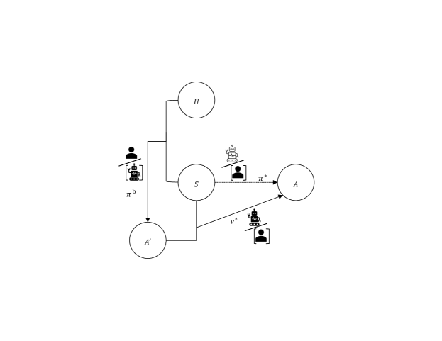
Figure 1: Graphical models for the data generating process under a behavior policy $\pi^{b}$, a standard optimal policy $\pi^{*}$ (dashed line) and a super policy $\nu^{*}$.

2.2 An Illustrative Example on Human-AI Interaction

Lemma 2.1 ensures the advantage of leveraging Human-AI interaction in the decision making, so-called “a blessing from Human-AI interaction". For instance, one can interpret the behavior policy $\pi^{b}$ as given by the AI system, which is capable of providing decisions based on massive information. As a human decision maker, despite the limitation to access all data information, she can make a better decision $\nu^{\ast}$ based on the recommendation given by the AI system. One can also interpret $\pi^{b}$ as the behavior policy given by the human agent which involves unique human insights. The super-policy $\nu^{*}$ learned by the machine utilizes such information and are guaranteed to outperform the human agents and the common policy that does not rely on human recommendations. In Section 2.4, we extend our framework to the setting where human and AI are iteratively interacting and making better decisions via finding the super-policy.

To further understand the appealing property of the proposed super-policy, consider the following toy example. Assume $S$ and $U$ independently follow a Bernoulli distribution with a success probability $0.5$. Suppose the action is binary (${\mathcal{A}}=\{0,1\}$) and the behavior policy satisfies $\mathbb{P}(A=1|S,U=1)=\mathbb{P}(A=0|S,U=0)=1-\varepsilon$ for some $0\leq\varepsilon\leq 1$. Let $R=8(A-0.5)(S-0.2)(U-0.3)$. In this example, the parameter $\varepsilon$ measures the degree of unmeasured confounding. When $\varepsilon=0.5$, the behavior policy does not depend on $U$ and the no-unmeasured-confounding assumption is satisfied. Otherwise, this condition is violated. In particular, when $\varepsilon=0$ or $1$, we can fully recover the latent confounder based on the recommended action. Table 1 summarizes the policy values of $\pi^{b}$, $\pi^{\ast}$ and $\nu^{\ast}$ under different $\varepsilon$, in which the super-optimality clearly holds.

Table 1: Policy values under different choices of $\varepsilon$ in the toy example. In general, ${\mathcal{V}}(\pi_{b})=0.6-1.2\varepsilon$, ${\mathcal{V}}(\pi^{\ast})=0.4$, ${\mathcal{V}}(\nu^{\ast})=|0.7-\varepsilon|+|\varepsilon-0.3|$. Bold values are the largest under different settings.

Policy Value	${\mathcal{V}}(\pi_{b})$	${\mathcal{V}}(\pi^{\ast})$	${\mathcal{V}}(\nu^{\ast})$
$\varepsilon=0.5$	0.0	0.4	0.4
$\varepsilon=0$	0.6	0.4	1.0
$\varepsilon=1$	-0.6	0.4	1.0

2.3 When is the super-optimality strict?

As seen from Table 1, when $\varepsilon=0$, the super-policy has the same performance as the standard optimal one $\pi^{\ast}$. This is due to the fact that the behavior policy $\pi^{b}$ does not provide additional information. To further understand when the strict improvement of $\nu^{\ast}$ over $\pi^{b}$ and $\pi^{\ast}$ happens, consider a binary-action setting with ${\mathcal{A}}=\{0,1\}$, where $1$ denotes the new treatment group and $0$ denotes the standard control. Define the conditional average treatment effect on the treated (CATT) and on the control (CATC) respectively as

$$\mathrm{CATT}(s)={\mathbb{E}}\{R(1)-R(0)\mid S=s,A=1\},$$

$$\mathrm{CATC}(s)={\mathbb{E}}\{R(1)-R(0)\mid S=s,A=0\}.$$

given any $s\in{\mathcal{S}}$. Then we have the following lemma, which explicitly characterizes the super-optimality of $\nu^{\ast}$ over $\pi^{\ast}$ and $\pi^{b}$.

Lemma 2.2.

The following three results hold.
(i) ${\mathcal{V}}(\nu^{*})>{\mathcal{V}}(\pi^{*})$ if and only if

$$\Pr\left(\left\{0<\pi^{b}(1|S)<1\right\}\cap\left\{\mathrm{CATT}(S)\times\mathrm{CATC}(S)<0\right\}\right)>0;$$

(ii) ${\mathcal{V}}(\nu^{*})>{\mathcal{V}}(\pi^{b})$ if and only if

$$\Pr\left(\left\{\mathrm{CATT}(S)<0\right\}\cup\left\{\mathrm{CATC}(S)>0\right\}\right)>0;$$

and (iii) ${\mathcal{V}}(\nu^{*})>\max\{{\mathcal{V}}(\pi^{*}),{\mathcal{V}}(\pi^{b})\}$ if and only if

$$\Pr\left(\left\{0<\pi^{b}(1|S)<1\right\}\cap\left\{\mathrm{CATT}(S)<0\right\}\cap\left\{\mathrm{CATC}(S)>0\right\}\right)>0;$$

Result (i) of Lemma 2.2 indicates that by treating $A$ as an additional feature, as long as $A$ is informative for achieving a better expected reward for some feature $S$, we have the strict improvement of $\nu^{\ast}$ over $\pi^{\ast}$. Meanwhile, Result (ii) of Lemma 2.2 implies that as long as the alternative action is better than the one recommended by $\pi^{b}$ for some feature $S$, strict improvement of $\nu^{\ast}$ over $\pi^{b}$ is guaranteed. Clearly, Result (iii) ensures the strict super-optimality when the previous two scenarios happen simultaneously.

2.4 Super RL for Sequential Decision Making

In this section, we introduce the super-policy for confounded sequential decision making and demonstrate its super-optimality. For any generic sequence $\{X_{t}\}_{t\geq 1}$, its realization $\{x_{t}\}_{t\geq 1}$ and its spaces $\{{\mathcal{X}}_{t}\}_{t\geq 1}$, we denote $X_{1:t}=(X_{1},\dots,X_{t})$, $x_{1:t}=(x_{1},\dots,x_{t})$ and $\mathcal{X}_{1:t}=\prod_{t^{\prime}=1}^{t}{\mathcal{X}}_{t^{\prime}}$.

Consider an episodic and confounded stochastic process denoted by ${\mathcal{M}}=(T,\mathcal{O},{\mathcal{U}},{\mathcal{A}},\mathcal{P},{\mathcal{R}})$, where the integer $T$ is the total length of horizon, $\mathcal{O}=\{\mathcal{O}_{t}\}_{t=1}^{T}$ and ${\mathcal{U}}=\{{\mathcal{U}}\}_{t=1}^{T}$ denote the spaces of observed and unobserved features respectively, ${\mathcal{A}}=\{{\mathcal{A}}_{t}\}_{t=1}^{T}$ denotes the action spaces across $T$ decision points, $\mathcal{P}=\{\mathcal{P}_{t}\}_{t=1}^{T}$ where each ${\mathcal{P}}_{t}$ denotes transition kernel from $\prod_{t^{\prime}=1}^{t}(\mathcal{O}_{t^{\prime}}\times{\mathcal{U}}_{t^{\prime}}\times{\mathcal{A}}_{t^{\prime}})\rightarrow\mathcal{O}_{t+1}\times{\mathcal{U}}_{t+1}$ at time $t$, and ${\mathcal{R}}$ denotes the set of rewards. The random process following ${\mathcal{M}}$ can be summarized as $\{O_{t},U_{t},A_{t},R_{t}\}_{t=1}^{T}$, where $O_{t}$ and $U_{t}$ correspond to the observed and latent features at time $t$, $A_{t}$ and $R_{t}$ denote the action and the reward at time $t$. We assume that $O_{t}$ is some noisy mapping of $U_{1:t}$ and satisfies that $O_{t}\mbox{$\perp\!\!\!\perp$}(O_{1:t-1},A_{1:t})|U_{1:t}$ for every $1\leq t\leq T$. For simplicity, we assume the action space is discrete and all rewards are uniformly bounded, i.e., $|R_{t}|\leq R_{\max}$. In the offline setting, we assume the observed action $A_{t}$ in the batch data is generated by some behavior policy $\pi^{b}_{t}:{\mathcal{U}}_{1:t}\times{\mathcal{A}}_{1:t-1}\rightarrow{\mathcal{P}}({\mathcal{A}}_{t})$ for $1\leq t\leq T$ and let $\pi^{b}=\{\pi^{b}_{t}\}_{t=1}^{T}$; Lastly, we denote the reward function as $r_{t}:\mathcal{U}_{1:t}\times\mathcal{A}_{1:t}\rightarrow\mathbb{R}$, i.e., $r_{t}={\mathbb{E}}[R_{t}|U_{1:t}=\bullet,A_{1:t}=\bullet]$.

Given the decision process ${\mathcal{M}}$ generated by the behavior policy, the objective of an agent is to learn an (in-class) optimal policy that can maximize the expected cumulative rewards. Nearly all existing works are focused on policies defined as a sequence of functions mapping from the past history (excluding the actions produced by the behavior agent) to a probability mass function over the action space ${\mathcal{A}}_{t}$. Specifically, let $\Pi\equiv\{\pi=\{\pi_{t}\}_{t=1}^{T}\,\mid\,\pi_{t}:\mathcal{O}_{1:t}\times{\mathcal{A}}_{1:t-1}\rightarrow{\mathcal{P}}(\mathcal{A}_{t})\}$. Then for any $\pi\in\Pi$, one can use the policy value to evaluate its performance, which is defined as

$${\mathcal{V}}(\pi)={\mathbb{E}}[V^{\pi}_{1}(O_{1},U_{1})],$$ (3)

where we use ${\mathbb{E}}$ to denote the expectation with respect to the initial data distribution. Here the value function $V^{\pi}_{t}$ is defined as for every $(o_{1:t},u_{1:t})\in\mathcal{O}_{1:t}\times{\mathcal{U}}_{1:t}$

$$\textstyle V^{\pi}_{t}(o_{1:t},u_{1:t})={\mathbb{E}}^{\pi}\left[\sum_{t^{\prime}=t}^{T}R_{t^{\prime}}|O_{1:t}=o_{1:t},U_{1:t}=u_{1:t}\right],$$ (4)

where ${\mathbb{E}}^{\pi}$ denotes the expectation with respect to the distribution whose action at each time $t$ follows $\pi_{t}$. Since $\{U_{t}\}_{t\geq 1}$ is not observed, previous works such as [32] focus on finding $\pi^{\ast}$ such that

$$\pi^{\ast}\in\operatorname{argmax}_{\pi\in\Pi}{\mathcal{V}}(\pi).$$

Similar to the contextual bandit setting, $\pi^{\ast}$ is not guaranteed outperforming $\pi^{b}$. Motivated by the discussions in Section 2.1, we consider a much larger policy class

$$\Omega\equiv\{\nu=\{\nu_{t}\}_{t=1}^{T}\,\mid\,\nu_{t}:\mathcal{O}_{1:t}\times{\mathcal{A}}_{1:t-1}\times{\mathcal{A}}_{1:t}\rightarrow{\mathcal{P}}(\mathcal{A}_{t})\},$$

where ${\mathcal{A}}_{1:t-1}$ represents the past actions taken by the policy $\nu$ up to $(t-1)$ decision points and ${\mathcal{A}}_{1:t}$ represents the actions generated by the behavior policy up to $t$ decision points. The policy class $\Omega$ reflects the iterative interaction between human and AI because either $\nu$ or $\pi^{b}$ can be regarded as human or AI. Therefore, we propose to learn a super policy $\nu^{\ast}$ such that

$$\nu^{\ast}\in\operatorname{argmax}_{\nu\in\Omega}{\mathcal{V}}(\nu),$$

which leverages human or machine expertise for enhanced decision making that maximizes ${\mathcal{V}}(\nu)$. By sequentially integrating historical and current actions of the behavioral agent into the decision-making process, the super policy leverage the iterative human-AI interaction, as illustrated in Figure 2.

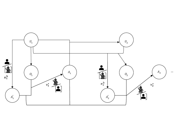
Figure 2: Graphical model for the sequential decision making under super policy $\nu^{*}$ by leveraging the offline data generated by the behavior policy with $T=2$. Here $\pi^{b}_{1}$ depends on $U_{1}$, $\pi^{b}_{2}$ depends on $U_{1},U_{2},A_{1}$; $\nu^{*}_{1}$ depends on $O_{1},A^{\prime}_{1}$, $\nu^{*}_{2}$ depends on $O_{1},O_{2},A_{1},A^{\prime}_{1},A_{2}^{\prime}$.

Similar as before, since the super-policy additionally uses the recommendation generated by the behavior policy that depends on the unobserved information, we expect the super-policy $\nu^{\ast}$ superior to both $\pi^{\ast}$ and $\pi^{b}$, which is shown below.

Theorem 2.1 (Super-Optimality).

${\mathcal{V}}(\nu^{*})\geq\max\{{\mathcal{V}}(\pi^{*}),{\mathcal{V}}(\pi^{b})\}$.

Given the appealing property of the super policy, in the following section, we discuss how to identify it using the offline data.

3 Causal Identification for Super Policies

Despite the appealing property of the proposed super policy, it is generally impossible to learn $\nu^{\ast}$ without any further assumptions, since for example, in the contextual bandit setting, the counterfactual effect ${\mathbb{E}}\left[R(a)|S=s,A=a^{\prime}\right]$ is not identifiable from the observed data due to unmeasured confounding. In this section, we extend the idea of proximal causal inference [52] to address the challenge posed by unmeasured confounding, and develop several nonparametric identification results for super policies within the contexts of the contextual bandit and the sequential setting.

3.1 Identification of Super Policies in Contextual Bandits

In the bandit setting, similar to [52], we assume the existence of certain action and reward proxies $Z\in{\mathcal{Z}}$ and $W\in{\mathcal{W}}$ in addition to $(S,A,R)$. These proxies are required to satisfy the following assumptions:

Assumption 1.

(a) $R\rotatebox[origin={c}]{90.0}{$\models$}Z|(S,U,A)$; (b) $W\rotatebox[origin={c}]{90.0}{$\models$}(Z,A)|(S,U)$, $W\cancel{\rotatebox[origin={c}]{90.0}{$\models$}}U|S$; (c) $R(a)\rotatebox[origin={c}]{90.0}{$\models$}A|(S,U)$ for $a\in{\mathcal{A}}$; (d) There exists a bridge function $q:{\mathcal{W}}\times{\mathcal{A}}\times{\mathcal{S}}\rightarrow\mathbb{R}$ such that

$${\mathbb{E}}\left[q(W,a,S)|U,S,A=a\right]={\mathbb{E}}\left[R|U,S,A=a\right].$$ (5)

Assumptions 1(a)-(b) are standard in proximal causal inference [36]. Assumptions 1(c), which is called latent unconfoundedness, is mild as we allow $U$ to be unobserved. The last assumption can be satisfied when some completeness and regularity conditions hold. See [35] and also Lemma 3.2 below for more details. The following identification result allows us to learn the super-policy $\nu^{\ast}$ from the observed data. We remark that this result is new and different from the standard proximal causal inference.

Lemma 3.1.

Under Assumption 1, we have ${\mathbb{E}}\left[R(a)|S=s,A=a^{\prime}\right]={\mathbb{E}}[q(W,a,S)|S=s,A=a^{\prime}],$ for every $(s,a,a^{\prime})$. Then for any $\nu\in\Omega$,

$${\mathcal{V}}(\nu)={\mathbb{E}}\left[\sum_{a\in{\mathcal{A}}}q(W,a,S)\nu(a|S,A)\right].$$

In practice, one may want to include as many confounders in the policy as possible to achieve the largest super-optimality. Hence under this proximal causal inference framework, with some abuse of notation, we further extend the policy class to $\Omega=\{\nu:{\mathcal{S}}\times{{\mathcal{Z}}}\times{\mathcal{A}}\rightarrow{\mathcal{P}}({\mathcal{A}})\}$ and consider the corresponding super-policy $\nu^{\ast}$ as

$$\nu^{\ast}(a^{\ast}|s,{z},a^{\prime})=1\quad\text{if}\quad a^{\ast}=\operatorname{argmax}_{a\in{\mathcal{A}}}{\mathbb{E}}\left[R(a)|S=s,{Z}={z},A=a^{\prime}\right],$$ (6)

In applications where the action proxy is no longer available in future decision making, (6) is reduced to (2). We remark that different from $Z$, $W$ is usually obtained after intervention, which should not be included in the super-policy. The next corollary allows us to identify $\nu^{\ast}$.

Corollary 3.1.

Under Assumption 1, the policy value under a given $\nu\in\Omega$ is given by ${\mathcal{V}}(\nu)={\mathbb{E}}\left[\sum_{a\in{\mathcal{A}}}q(W,a,S)\nu(a|S,A,{Z})\right]$. In addition, the optimal policy $\nu^{\ast}$ is given by

$$\nu^{\ast}(a^{\ast}|s,{z},a^{\prime})=1\quad\text{if}\quad a^{\ast}=\operatorname{argmax}_{a\in{\mathcal{A}}}{\mathbb{E}}\left[q(W,a,S)|S=s,{Z}={z},A=a^{\prime}\right].$$ (7)

It can be seen from Corollary 3.1 that to identify the super-policy, it remains to estimate the bridge function $q$ defined in Assumption 1(d). One can impose the following completeness condition to consistently estimate it.

Assumption 2 (Completeness).

(a) For any squared-integrable function $g$ and for any $(s,a)\in{\mathcal{S}}\times{\mathcal{A}}$, ${\mathbb{E}}[g(U)|Z,S=s,A=a]=0$ almost surely if and only if $g(U)=0$ almost surely.
(b) For any squared-integrable function $g$ and for any $(s,a)\in{\mathcal{S}}\times{\mathcal{A}}$, ${\mathbb{E}}[g(Z)|W,S=s,A=a]=0$ almost surely if and only if $g(Z)=0$ almost surely.

Completeness is a technical assumption commonly adopted in value identification problems. It can be satisfied by a wide range of models and distributions in statistics and econometrics [e.g. 13, 11, 52]. For (a), it indicates that $Z$ should have sufficient variability compared to the variability of $U$, which helps to make (8) in the following hold when replacing $Z$ with $U$. The condition (b) is mainly proposed for ensuring the existence of solution for (8).

Lemma 3.2.

Under Assumptions 1-2 and some regularity conditions (see Assumption 9 in Section A in Appendix, solving the following linear integral equation

$${\mathbb{E}}\left[q(W,a,S)|Z,S,A=a\right]={\mathbb{E}}\left[R|Z,S,A=a\right],$$ (8)

for every $a\in{\mathcal{A}}$ with respect to $q$ gives a valid bridge function that satisfies Assumption 1(d).

Built upon Corollary 3.1 and Lemma 3.2, we can estimate the bridge function $q$ using the observed data and therefore obtain an estimation of super policy $\nu^{*}$. See Section 4.1 for more details and the proposed algorithm.

3.2 Identification of Super Policies in Sequential Decision Making

Next, we discuss how to identify $\nu^{\ast}$ in the sequential setting. It is worth mentioning that it is very challenging to identify the super-policy in the confounded sequential decision-making setting as we aim to include two sets of past actions for policy search, i.e., those generated by the behavior policy and by the super-policy. In the following, we introduced two approaches to identify policy values with the help of some proxy variables. Both are motivated by the recent development of identifying off-policy value in the confounded POMDPs [3, 53, 46, 34]. One approach requires an additional proxy variable which is independent of the past action at each decision point (Section 3.2.1) and an efficient learning algorithm can be developed under the memoryless assumption (Section 4.2). The other approach, which does not need the proxy variables, builds on the current data generating process but with the loss of an efficient learning algorithm (Section 3.2.2).

3.2.1 Identification of Super-Policies via Q-bridge Functions

In this subsection, we develop the framework for the identification of super-policies in the confounded sequential decision making settings via $Q$-bridge functions. Note that in our policy class $\Omega$, the policy $\nu_{t}$ depends on two sets of actions where one set of actions is induced by the policy $\{\nu_{t^{\prime}}\}_{t^{\prime}=1}^{t-1}$ and the other set of actions is generated by the behavoir policy $\{\pi^{b}_{t^{\prime}}\}_{t^{\prime}=1}^{t}$. To distinguish two sources of actions, in the sequel, we use $A_{t}$ to represent the observed action (the action taken by the behavior agent) and $A^{\nu}_{t}$ to represent the action induced by $\nu$. For notation simplicity, in the following, we define $Z_{t}=\{O_{1:t},A^{\nu}_{1:t-1}\}\in\mathcal{Z}_{t}$, where $\mathcal{Z}_{t}:=\mathcal{O}_{1:t}\times{\mathcal{A}}_{1:t-1}$. To start with, we make the following assumptions.

Assumption 3.

There exists a sequence of reward proxy variables $\{W_{t}\}_{t=1}^{T}$ such that $W_{t}\rotatebox[origin={c}]{90.0}{$\models$}A_{t}\mid(U_{1:t},O_{1:t},A_{1:t-1})$ and $W_{t}\cancel{\rotatebox[origin={c}]{90.0}{$\models$}}U_{1:t}|(O_{1:t},A_{1:t-1})$, for $1\leq t\leq T$.

Assumption 3 requires the existence of a sequence of proxy variables $\{W_{t}\}_{t=1}^{T}$, which are not affected by the previous action but correlated with the past hidden information. If one does not wish to assume an additional proxy variable, alternatively one may set $W_{t}$ as $O_{t}$ and take $Z_{t}=\{O_{1:t-1},A^{\nu}_{1:t-1}\}\in{\mathcal{Z}}_{t}$. Then Assumption 3 automatically holds under the current problem setting. However, in this case, the super policy $\nu_{t}$ needs to be defined over $\mathcal{O}_{1:t-1}\times{\mathcal{A}}_{1:t-1}\times{\mathcal{A}}_{1:t}$, which excludes the current observation $O_{t}$. In the following discussion, we assume the existence of $\{W_{t}\}_{t=1}^{T}$. To identify ${\mathcal{V}}(\nu)$ and ultimately $\nu^{\ast}$ under unmeasured confounding, we assume the existence of a class of $Q$-bridge functions below. Similar to the discussion in Section 3.1, the existence of such brdige functions can be satisfied under some completeness and regularity assumptions (see Assumptions 10 and 11 in Appendix).

Assumption 4.

There exists a class of $Q$-bridge functions $\{q^{\nu}_{t}\}_{t=1}^{T}$, where $q^{\nu}_{t}$ is defined over ${\mathcal{W}}\times{\mathcal{Z}}_{t}\times{\mathcal{A}}_{1:t}\times{\mathcal{A}}$ for $t=1,\dots,T-1$, such that for every $(u_{1:t},o_{1:t},a_{1:t})\in{\mathcal{U}}_{1:t}\times\mathcal{O}_{1:t}\times{\mathcal{A}}_{1:t}$ and every $a_{1:t}\in{\mathcal{A}}_{1:t}$,

$$\textstyle{\mathbb{E}}^{\nu}\left[\sum_{t^{\prime}=t}^{T}R_{t^{\prime}}|U_{1:t},O_{1:t},A^{\nu}_{1:t-1},A_{1:t}=a_{1:t}\right]={\mathbb{E}}\left[\sum_{a\in{\mathcal{A}}}q^{\nu}_{t}(W_{t},Z_{t},a_{1:t},a)\nu_{t}(a\mid Z_{t},a_{1:t})|U_{1:t},O_{1:t},A^{\nu}_{1:t-1}\right],$$ (9)

where the Q-bridge function of the last step $q^{\nu}_{T}$ defined over over ${\mathcal{W}}\times{\mathcal{Z}}_{T}\times{\mathcal{A}}$ satisfies

$$\textstyle{\mathbb{E}}^{\nu}\left[R_{T}|U_{1:T},O_{1:T},A^{\nu}_{1:T-1},A_{1:T}=a_{1:T}\right]={\mathbb{E}}\left[\sum_{a\in{\mathcal{A}}}q^{\nu}_{T}(W_{T},Z_{t},a)\nu_{t}(a\mid Z_{T},a_{1:T})|U_{1:T},O_{1:T},A^{\nu}_{1:T-1}\right].$$ (10)

Let $O_{0}$ denote some pre-collected observation before the decision process initiates. We impose the following additional assumption for $O_{0}$.

Assumption 5.

$(R_{t},W_{t+1},W_{t},O_{t+1},U_{t+1})\mbox{$\perp\!\!\!\perp$}O_{0}|U_{1:t},O_{1:t},A_{1:t}$, for $1\leq t\leq T-1$.

The role of $O_{0}$ is similar to the role of the action proxy $Z$ in the setting of contexual bandits. Given all the history and current state variables and actions, we assume it to be independent of the current reward ($R_{t}$) and the current and future proxy variables ($W_{t}$ and $W_{t+1}$). In practice, state variables at the next step ($U_{t+1},O_{t+1}$) often solely depend on the history and current state variables and actions, leading to a natural independence between $O_{0}$ and $(U_{t+1},O_{t+1})$.

Given aforementioned assumptions, we have the following identification result.

Theorem 3.1.

Suppose Assumptions 3-5, and certain completeness and regularity conditions (Assumptions 10 and 11) in Section B in Appendix hold. Let $q^{\nu}_{T+1}=0$. At time $T$, the Q-brige function $q^{\nu}_{T}(\cdot,\cdot,\cdot)$ is obtained via solving

$${\mathbb{E}}\left\{q^{\nu}_{T}(W_{T},(O_{1:T},A_{1:T-1}),A_{T})-R_{T}|(O_{1:T},A_{1:T-1}),O_{0},A_{T}\right\}=0.$$ (11)

From $t=T-1,\dots,1$, the Q-bridge function$q_{t}$ can be obtained via solving the following linear integral equation. In particular, for any $a_{1:t}\in{{\mathcal{A}}}_{1:t}$, $q^{\nu}_{t}(\cdot,\cdot,a_{1:t},\cdot)$ is the solution to

$${\mathbb{E}}\left\{q^{\nu}_{t}(W_{t},(O_{1:t},A_{1:t-1}),{a}_{1:t},A_{t})-R_{t}-\right.\\ \left.\sum_{a\in{\mathcal{A}}}q^{\nu}_{t+1}(W_{t+1},(O_{1:t+1},A_{1:t}),({a}_{1:t},A_{t+1}),a)\nu_{t+1}(a\mid(O_{1:t+1},A_{1:t}),({a}_{1:t},A_{t+1}))|(O_{1:t},A_{1:t-1}),O_{0},A_{t}\right\}=0,$$ (12)

Then the policy value of $\nu\in\Omega$ can be identified as

$${\mathcal{V}}(\nu)={\mathbb{E}}\left[\sum_{a\in{\mathcal{A}}}q^{\nu}_{1}(W_{1},O_{1},A_{1},a)\nu_{1}(a\mid O_{1},A_{1})\right].$$ (13)

In Assumption 4, different from the definition of $q_{t}^{\nu}$ for $t<T$, $q^{\nu}_{T}$ does not depend on the actions from actions $a_{1:T}$ produced from the behavior policy. The intuitive reason behind it is that at the last step $T$, as long as all the state variables $U_{1:T},O_{1:T}$ and actions $A_{1:T}^{\nu}$ produced by the policy $\nu$ are conditioned, the reward $R_{T}$ does not depend on the actions produces by the behavior policy. However, for $t<T$, the later rewards $R_{t+1},\dots,R_{T}$ that produced by the policy $\nu$ will depend on the policies $\nu_{t+1},\dots,\nu_{T}$, and therefore actions $a_{1:t}$ produced by the behavior policy, even though conditioning on $U_{1:t},O_{1:t}$ and $A_{1:t}^{\nu}$.

3.2.2 Identification of Super-Policies via V-bridge Functions

In Section 3.2.1, we discuss how to identify the policy value via Q-bridge functions assuming the existence of certain observations $W_{t}$ that can serve as proxy variables and are conditionally independent of the current action. As commented earlier, this condition can be relaxed by setting $W_{t}=O_{t}$ and restricting the dependence between the current policy $\nu_{t}$ and current observation $O_{t}$. However, this exclusion may not be satisfactory because the current observation may be the most informative in the decision making. In the following, we provide a remedy for addressing this limitation under a new identification result. We adopt the same notations as defined in Section 3.2.1 for $A_{t}$ and $A^{\nu}_{t}$. Also, we assume there exists some pre-collected observation $O_{0}$ satisfying the following assumption.

Assumption 6.

$O_{o}\mbox{$\perp\!\!\!\perp$}(R_{t},O_{t+1},O_{t},U_{t+1})|U_{1:t},O_{1:t-1},A_{1:t}$ for $t=1,\dots,T$.

Different from Assumption 5, here we particularly require that $O_{0}$ is independent of current observation $O_{t}$ given $U_{1:t},O_{1:t-1},A_{1:t}$. In addition, we also assume the existence of the value bridge functions $\{b^{\nu}_{t}\}_{t=1}^{T}$ satisfying the following condition.

Assumption 7.

For any history-dependent policy $\nu\in\Omega$, there exist a series of value bridge functions $b^{\nu}_{t}$ over ${\mathcal{A}}\times(\mathcal{O}_{1:t-1}\times{\mathcal{A}}_{1:t-1})\times\mathcal{O}_{t}\times{{\mathcal{A}}}_{1:t}$, $t=1,\dots,T$ such that for any $a_{1:t}\in{\mathcal{A}}_{1:t}$ and $a\in{\mathcal{A}}_{t}$,

$${\mathbb{E}}^{\nu}\left\{\left(\sum_{t^{\prime}=t}^{T}R_{t^{\prime}}\right)\nu_{t}(a\mid O_{t},(O_{1:t-1},A^{\nu}_{1:t-1}),a_{1:t})|U_{1:t},(O_{1:t-1},A^{\nu}_{1:t-1}),A_{1:t}=a_{1:t},A^{\nu}_{t}=a\right\}\\ ={\mathbb{E}}^{\nu}\left\{b^{\nu}_{t}(a,(O_{1:t-1},A^{\nu}_{1:t-1}),O_{t},a_{1:t})\mid U_{1:t},(O_{1:t-1},A^{\nu}_{1:t-1})\right\}.$$

The following theorem identifies the super policies via the $V$-bridge functions $\{b^{\nu}_{t}\}_{t=1}^{T}$.

Theorem 3.2.

Under Assumption 6-7 and the completeness assumption (Assumption 12 in Appendix), the value bridge function $b^{\nu}_{t}(a,\cdot,a_{1:t})$ can be obtained by solving

$${\mathbb{E}}\left\{b^{\nu}_{t}(a,(O_{1:t-1},A_{1:t-1}),O_{t},a_{1:t})\right.\\ \left.-\left[R_{t}+\sum_{a^{\prime}\in{\mathcal{A}}}b^{\nu}_{t+1}(a^{\prime},(O_{1:t},A_{1:t}),O_{t+1},(a_{1:t},A_{t+1}))\right]\nu_{t}(a\mid(O_{1:t-1},A_{1:t-1}),O_{t},a_{1:t})\right.\\ \left.|O_{o},(O_{1:t-1},A_{1:t-1}),A_{t}=a\right\}=0,$$ (14)

where $b_{T+1}$ is a zero function. Furthermore, we can identify the policy value as

$${\mathcal{V}}(\nu)={\mathbb{E}}\left[\sum_{a\in{\mathcal{A}}}b^{\nu}_{1}(a,O_{1},A_{1})\right].$$

Based on Theorem 3.2, we could estimate $b_{t}^{\nu}$ from the observed data. However, $b^{\nu}_{t}(a,\cdot,a_{1:t})$ depends on $\{\nu_{t}^{\prime}\}_{t^{\prime}\geq t}$ intricately as shown in (14). As a result, it can only be estimated when the policy $\nu$ is given explicitly. Therefore, developing an efficient algorithm to learn the optimal policy sequantially can be quite challenging in this case. A greedy algorithm that jointly optimizes $\{\nu_{t}\}_{t=1}^{T}$ can be adopted to search for the optimal policy, which requires extensive computational resourse and time. In this paper, we do not investigate further in the development of algorithm for policy learning using value bridge functions and leave it as future work.

4 Estimations and Algorithms

In this section, we introduce our super-policy learning algorithms based on the identification results developed in Section 3.1 and Section 3.2, and provide corresponding estimation procedures.

4.1 Confounded Contextual Bandits: Algorithm Development

In Algorithm 1, we summarize the steps in learning the super policy using the observed data for contextual bandits. The first key step is to estimate the bridge function $q$ by the linear integral equation stated in Lemma 3.2. The second key step is to estimate the projection term ${\mathbb{E}}[\hat{q}(W,S,a)|S=s,Z=z,A=a^{\prime}]$ for every $a\in{\mathcal{A}}$, using the estimated bridge function $\hat{q}$.

1 Input: Data $\mathcal{D}=(S_{i},Z_{i},A_{i},R_{i},W_{i})_{i=1}^{n}$.

2 Obtain the estimation of the bridge function $\hat{q}$ by solving the estimation equation (8) using data $\mathcal{D}$

3 Implement any supervised learning method for estimating ${\mathbb{E}}\left[\hat{q}(W,S,a)|S,Z,A\right]$.

4 Compute $a^{\ast}=\operatorname{argmax}_{a\in{\mathcal{A}}}\hat{\mathbb{E}}\left[\hat{q}(W,S,a)|S=s,Z=z,A=a^{\prime}\right]\quad\forall(s,z,a^{\prime})\in{\mathcal{S}}\times{\mathcal{Z}}\times{\mathcal{A}}$.

Output: $\hat{\nu}^{\ast}$ with $\hat{\nu}^{\ast}(a^{\ast}|s,z,a^{\prime})=1$ and $\hat{\nu}^{\ast}(\tilde{a}|s,z,a^{\prime})=0$ for $\tilde{a}\neq a^{\ast}$.

Algorithm 1 Learning Algorithm for the contextual bandits under unmeasured confounding

When ${\mathcal{S}}\times{\mathcal{Z}}\times{\mathcal{A}}\times{\mathcal{W}}$ are all finite and discrete, the bridge function and the projection term can be straightforwardly estimated via empirical average. In the following, we focus on the case where the function approximation is needed. Specifically, we adopt the procedure for solving the conditional moment estimation procedure in [12], and propose to estimate $Q$-bridge function by

$$\hat{q}:=\operatorname*{arg\,min}_{q^{\prime}\in{\mathcal{Q}}}\left\{\sup_{g\in{\mathcal{G}}}\tilde{\Psi}(q^{\prime},g)-\lambda\left(\|g\|^{2}_{{\mathcal{G}}}+\frac{U}{\Delta^{2}}\|g\|_{2,n}^{2}\right)\right\}+\lambda\mu\|q^{\prime}\|_{{\mathcal{Q}}}^{2},$$ (15)

where $\tilde{\Psi}(q^{\prime},g)=\frac{1}{n}\sum_{i=1}^{n}\left\{q^{\prime}(W_{i},S_{i},A_{i})-R_{i}\right\}g(Z_{i},S_{i},A_{i})$; $\|g\|_{2,n}^{2}=n^{-1}\sum_{i=1}^{n}g^{2}(Z_{i},S_{i},A_{i})$ for $g\in{\mathcal{G}}$; ${\mathcal{Q}}$ is the imposed model for $q$ (the solution of (8)); ${\mathcal{G}}$ is the function space where the test functions $g$ come from. In addition, $\lambda,\mu,\Delta,U>0$ are some tuning parameters. The motivation behind (15) is that when $\lambda$, $\lambda\mu\rightarrow 0$ and $\lambda U/\Delta\asymp 1$, the solution of the following population-version min-max optimization problem

$$\operatorname*{arg\,min}_{q^{\prime}\in{\mathcal{Q}}}\sup_{g\in{\mathcal{G}}}{\mathbb{E}}\left\{[q^{\prime}(W,S,A)-R]g(Z,S,A)-\frac{1}{2}g^{2}(Z,S,A)\right\}$$

is equivalent to the solution of following optimization problem

$$\operatorname*{arg\,min}_{q^{\prime}\in{\mathcal{Q}}}{\mathbb{E}}\left\{{\mathbb{E}}[q^{\prime}(W,S,A)-R|Z,S,A]^{2}\right\},$$

when the space ${\mathcal{G}}$ of testing functions is rich enough.

In practice, spaces ${\mathcal{Q}}$ and ${\mathcal{V}}$ are user-specified. To increase flexibility, ${\mathcal{Q}}$ and ${\mathcal{V}}$ can be implemented using growing linear sieves, reproducing kernel Hilbert spaces (RKHSs) and deep neural networks. When ${\mathcal{Q}}$ and ${\mathcal{V}}$ are taken as RKHSs, the optimization seems infinite-dimensional. However, due to the well-known representer theorem, one can show that there exists a closed-form solution that lies in a finite-dimensional space. For more information on deriving the closed-form solution, as well as guidance on hyper-parameter tuning and strategies to improve computational efficiency, we refer readers to Section E.3 of [12].

Meanwhile, the conditional moment framework can be adopted to obtain the projection term. Here, we propose to perform the estimation via the empirical risk minimization:

$$\hat{g}(\cdot,\cdot,\cdot\ ;\ \hat{q}(\cdot,\cdot,a)):=\operatorname*{arg\,min}_{g\in{\mathcal{G}}}\frac{1}{n}\sum_{i=1}^{n}\left[g(S_{i},Z_{i},A_{i})-\hat{q}(\cdot,\cdot,a)\right]^{2}+\mu^{\prime}\|g\|_{{\mathcal{G}}}^{2},$$ (16)

where $\hat{q}$ is defined in (15) and $\mu^{\prime}>0$ is a tuning parameter. Similarly, one can take the pre-specified space ${\mathcal{G}}$ in (16) as growing linear sieves and RKHSs, which result in typical penalized spline regression and kernel ridge regression respectively.

4.2 Confounded Sequential Decision Making: Algorithm Development

Given the identification results in Theorems 3.1 (or Theorem 3.2), to obtain the super-policy $\nu^{\ast}$, one solution is to directly search the optimal policy over the space of super-policies that maximize the estimated value, i.e.,

$$\hat{\nu}=\operatorname{argmax}_{\nu\in\Omega}\widehat{{\mathcal{V}}}(\nu),$$

where $\widehat{{\mathcal{V}}}(\nu)$ is obtained by iteratively estimating $q_{t}^{\nu}$ through (12) (or $b^{\nu}_{t}$ through (14)) from $t=T$ to $t=1$ with fixed $\nu$.

However, when $T$ is large and models imposed for estimating bridge functions are complex (e.g., deep neural networks), direct optimizing $\widehat{{\mathcal{V}}}(\nu)$ requires extensive computational power. Therefore, we restrict our focus to a special case of the sequential setting described in Section 3.2.1, under which a more practical algorithm with theoretical guarantee can be derived. We leave the development of efficient algorithms under general settings as future work. Motivated by Theorem 3.1, we propose a fitted-Q-iteration (Q-learning) type algorithm (Algorithm 2) for practical implementation. In particular, Algorithm 2 has the theoretical guarantee (which we will discuss in Section D) under the following memoryless assumption.

Assumption 8 (Memoryless Unmeasured Confounding).

For $2\leq t\leq T$, $W_{t}\rotatebox[origin={c}]{90.0}{$\models$}U_{1:(t-1)}|(O_{1:t},A_{1:t})$, $A_{t}\rotatebox[origin={c}]{90.0}{$\models$}A_{1:t-1}|(U_{1:t},O_{1:t})$. At the last step $T$, we additionally assume $(U_{T},W_{T})\rotatebox[origin={c}]{90.0}{$\models$}A_{1:T-1}|(U_{1:T-1},O_{1:T})$.

The memoryless assumption plays an important role in deriving the algorithm wherein policies are learned sequentially, starting from the last step and working backward. Similar conditions have been commonly imposed in the literature to handle unmeasured confounding in a sequential setting [21, 15, 47, 60]. Mainly, it ensures that the projection step guarantees the optimality under the distributions regarding to both the behavior policy and the induced policy.

1 Input: Data $\mathcal{D}=\{{\mathcal{D}}_{t}\}_{t=1}^{T-1}$ with ${\mathcal{D}}_{t}=\{(O_{i,1:t},A_{i,1:t},R_{i,t},W_{i,t},O_{i,t+1},A_{i,t+1},W_{i,t+1})\}_{i=1}^{n}$.

2 Let $\hat{q}_{T+1}=0$ and $\hat{\nu}^{\ast}_{T}$ be an arbitrary policy.

3 At time $T$, obtain $\hat{q}_{T}$ for $q_{T}$ by solving (11). Compute $\hat{\mathbb{E}}[\hat{q}_{T}(W_{T},(O_{1:T},a^{\nu}_{1:T-1}),A_{T},a^{\nu})|O_{1:T}=o_{1:T},A_{1:T}=a_{1:T}]$ for $a^{\nu}\in{\mathcal{A}}$ and $a^{\nu}_{1:T-1}\in{\mathcal{A}}_{1:T-1}$ using any supervised learning method and obtain the estimated super policy $\hat{\nu}^{\ast}_{T}$ as $\hat{\nu}^{\ast}_{T}(a^{\ast}|o_{1:T},a^{\nu}_{1:T-1},a_{1:T})=\mathbbm{1}\left\{\operatorname{argmax}_{a\in{\mathcal{A}}}\hat{\mathbb{E}}[\hat{q}_{T}(W_{T},(O_{1:T},a^{\nu}_{1:T-1}),a)|O_{1:T}=o_{1:T},A_{1:T}=a_{1:T}]\right\}$ for any $a^{\nu}_{1:T-1}\in{\mathcal{A}}_{1:T-1}$.

4 Repeat for $t=T-1,\dots,1$:

5 Obtain an estimator $\hat{q}_{t}$ for $q_{t}$ by solving (12) using data $\mathcal{D}_{t}$ and $\hat{q}_{t+1}$ obtained from the last iteration.

6 Compute $\hat{\mathbb{E}}[\hat{q}_{t}(W_{t},(O_{1:t},A_{1:t-1}),(a_{1:t-1},A_{t}),a)|O_{1:t},A_{1:t}]$ for $a\in{\mathcal{A}}$ and $a_{1:t-1}\in{\mathcal{A}}_{1:t-1}$ using any supervised learning method and obtain the estimated super policy $\hat{\nu}^{\ast}_{t}$ as $\hat{\nu}^{\ast}_{t}(a^{\ast}|o_{1:t},a^{\nu}_{1:t-1},(a_{1:t-1},a_{t}))=\mathbbm{1}\left\{\operatorname{argmax}_{a\in{\mathcal{A}}}\hat{\mathbb{E}}[\hat{q}_{t}(W_{t},(O_{1:t},A_{1:t-1}),(a_{1:t-1},A_{t}),a)|O_{1:t}=o_{1:t},A_{1:t-1}=a^{\nu}_{1:t-1},A_{t}=a_{t}]\right\}$ for any $a_{1:t-1}\in{\mathcal{A}}_{1:t-1}$.

Output: $\hat{\nu}^{\ast}=\{\hat{\nu}^{\ast}_{t}\}_{t=1}^{T}$.

Algorithm 2 Super RL for the confounded POMDP

In Algorithm 2, the iteration is conducted from the final time step $t=T$ to the first time step $t=1$. At each iteration $t$, there are two main steps. One is to estimate the $Q$-bridge function $q_{t}$ and the other is to perform the projection. We take similar procedures as described in Section 4.1 to perform these two steps. In the step of estimating the $Q$-bridge function, we follow the construction in [12] to derive the estimators. We construct the objective function for the $Q$-bridge function at the last step $T$ based on (11). For the steps $t<T$ and for every combination of $a_{1:t}$, we construct the objective function based on (12) to learn the $Q$-bridge function $q^{\nu}_{t}$, where we replace $\nu_{t+1}$ and $q^{\nu}_{t+1}$ with the estimated ones ($\hat{\nu}_{t+1}$ and $\hat{q}^{\nu}_{t+1}$ ) obtained from the previous step. For the projection step, it performs differently at step $T$ and steps $t<T$ as shown in Line 3 and Line 6 in Algorithm 2. In particular, at the last step $T$, the dependence of the policy on actions produced by the behavior agents ($a_{1:T}$) is done by conditioning the last step $Q$-bridge function on the observed actions $A_{1:T}$. At the steps $t<T$, the dependence of the policy on $a_{1:t-1}$ is directly through the input $a_{1:t-1}$ of the $Q$-bridge function $q^{\nu}_{t}$; the dependence on $a_{t}$ is through conditioning on the observed action $A_{t}$. A major reason for such difference in the projection steps is that the Q bridge function at the last step does not depend on the actions produced by the behavior actions $a_{1:T}$. The conditioning set $A_{1:T}$ in the projection step plays the role as the actions produced by the behavior policy, and through doing this we could learn the policy at the last step that depends not only on the previous taken actions but also on the actions produced by the behavior policy as well. Same implementation procedures as discussed in Section 4.1 can be used. In Section F.1 in Appendix, we list implementation details for these two steps.

5 Super-policy Learning with Regret Guarantees

In this section, we establish the finite-sample regret bounds for algorithms developed in Section 4. In particular, we focus on deriving the finite-sample upper bound for the regret of finding the super-policy in both contextual and sequential settings. The regret of any generic policy $\widetilde{\nu}$ is defined as

$$\text{Regret}(\widetilde{\nu})\equiv{\mathcal{V}}(\nu^{\ast})-{\mathcal{V}}(\widetilde{\nu}).$$ (17)

Due to space constraints, we present the contextual bandits results in the main paper. The regret bounds for the sequential setting are provided in Section D in Appendix. Specifically, we derive the regret bound for Algorithm 2 under the memoryless setting discussed in Section 4.2.

Let $\hat{\nu}^{\ast}$ denote the output of Algorithm 1 which relies on the estimation of the bridge function $q$ given by (8). Define the $\mathcal{L}_{2}$ norm of a generic function $f$ as $\|f\|_{2}\equiv\sqrt{{\mathbb{E}}[f^{2}]}$. Let $g(S,Z,A\ ;f)\equiv{\mathbb{E}}[f(W,S)\mid S,Z,A]$ for any $f$ defined over ${\mathcal{W}}\times{\mathcal{S}}$. For a given projection estimator $\hat{\mathbb{E}}$, let $\hat{g}(S,Z,A\ ;f)\equiv\hat{\mathbb{E}}[f(W,S)\mid S,Z,A]$ denote the corresponding estimator. Let

$$p_{\max}=\sup_{u,s,z,a^{\prime},\nu\in\Omega}\frac{\sum_{a\in{\mathcal{A}}}\pi_{b}(A=a\mid U=u,S=s)\nu(A^{\prime}=a^{\prime}\mid Z=z,S=s,A=a)}{\pi_{b}(A^{\prime}=a^{\prime}\mid U=u,S=s)}.$$

Define the projection error as $\xi_{n}:=\sup_{q\in{\mathcal{Q}},a\in{\mathcal{A}}}\left\|g[\cdot,\cdot,\cdot\ ;\ q(\cdot,\cdot,a)]-\hat{g}[\cdot,\cdot,\cdot\ ;\ q(\cdot,\cdot,a)]\right\|_{2},$ and the bridge function estimation error as $\zeta_{n}:=\left\|q-\hat{q}\right\|_{2}.$ The following Lemma shows that the regret bound can be controlled through bounding the $Q$ function estimation error and the projection estimation error.

Lemma 5.1.

Suppose $q$ belongs to the function class ${\mathcal{Q}}\subset{\mathcal{W}}\times{\mathcal{S}}\times{\mathcal{A}}$. Then we obtain the following regret decomposition

$$\text{Regret}(\hat{\nu}^{\ast})\leq 2(\xi_{n}+p_{\max}\zeta_{n}).$$

Lemma 5.1 indicates that the error bound consists of two compoennts: the estimation error for the bridge function and the estimation error for the projection step. Suppose $\hat{q}$ and the projection estimator are computed by the estimation procedures described in Section 4.1. When ${\mathcal{Q}}$ (the function space for $q$) and ${\mathcal{G}}$ (the function space for test functions and the function space for the projected function) are VC-subgraph classes, we have the following theorem for the regret guarantee. Results when ${\mathcal{G}}$ and ${\mathcal{Q}}$ are reproducing kernel Hilbert spaces (RKHSs) are provided Section F.4 in Appendix.

Theorem 5.1.

If the star-shaped spaces ${\mathcal{G}}$ and ${\mathcal{Q}}$ are VC-subgraph classes with VC dimensions $\mathbb{V}({\mathcal{G}})$, and $\mathbb{V}({\mathcal{Q}})$ respectively. Under assumptions in Theorems F.2 and F.5, with probability at least $1-\delta$,

$$\text{Regret}(\hat{v}^{\ast})\lesssim n^{-1/2}p_{\max}\sqrt{\log(1/\delta)+\max\left\{\mathbb{V}({\mathcal{G}}),\mathbb{V}({\mathcal{Q}})\right\}},$$

where for any two positive sequences $\{a_{n}\}_{n}$, $\{b_{n}\}_{n}$, $a_{n}\lesssim b_{n}$ means that there exists some universal constant $C>0$ such that $a_{n}\leq Cb_{n}$ for any $n$.

Theorem 5.1 provides the finite-sample regret bound for the super-policy learning algorithm under the setting of confounded contextual bandits. The bound is determind by the sample size $n$, the overlap quantity $p_{\max}$ and function spaces $\mathcal{Q}$ and $\mathcal{G}$. Suppose $p_{\max}$ is bounded by a constant and the VC dimensions are $K$, then the derived regret bound achieves the rate $\sqrt{K/n}\log n$.

6 Simulations

6.1 Simulation Study for Contextual Bandits

In this section, we conduct two simulation studies to evaluate the performance of the proposed super-policy. The first one is a contextual bandit example with discrete feature values. We aim to demonstrate the super-policy performs better when the behavior policy reveals more information about the unmeasured confounders. The second one is a contextual bandit example with a continuous state space. It is used to demonstrate the performance of our algorithm using the bridge function.

A contextual bandit example with discrete feature values: Similar to the toy example described in Section 2.1, we take $S$ and $U$ as independent binary variables such that $\Pr(S=1)=0.5$ and $\Pr(U=1)=0.5$. The binary action $A$ is generated by the following conditional probabilities

$$\Pr(A=1\mid U=0)=\epsilon,\qquad\Pr(A=1\mid U=1)=1-\epsilon,$$

with different choices of $\epsilon\in[0,1]$. The larger the $|\epsilon-0.5|$ is, the more information of $U$ is revealed in the observed action $A$. Both the reward proxy $W$ and the action proxy $Z$ are binary and are generated according to the following conditional probabilities

$$\Pr(W=1\mid U=0)=0.4,\qquad\Pr(W=1\mid U=1)=0.6;$$

$$\Pr(Z=1\mid U=0)=0.4,\qquad\Pr(Z=1\mid U=1)=0.6.$$

Moreover, $W$ and $Z$ are conditionally independent given $U$. The observed reward is computed by $R=(U-0.5)(A-0.5)+\epsilon$ where $\epsilon\sim N(0,0.5)$.

Three types of policy classes are considered.

1. Sonly: $\mathcal{S}\rightarrow\mathcal{P}(\mathcal{A})$. The policy only depends on the observed state $S$.

2. SZonly: $\mathcal{S}\times\mathcal{Z}\rightarrow\mathcal{P}(\mathcal{A})$. The policy depends on on the observed state $S$ and the action proxy $Z$.

3. Super: $\mathcal{S}\times\mathcal{Z}\times\mathcal{A}\rightarrow\mathcal{P}(\mathcal{A})$. The super-policy class where the policy depends on the observed state $S$, the action proxy $Z_{t}$, and observed action $A$.

We implement Algorithm 1 to estimate the corresponding optimal policies for different policy classes. Note that for Sonly and SZonly, we perform the projection step (line 4) by conditioning on $S$ and $(S,Z)$ respectively. Since the feauture values are discrete, we use the empirical averages to approximate all the conditional expectations. In this simulation study, we consider the sample size $n=5000$. As Table 2 shows, the super-policy produces smallest regret as $\epsilon$ deviates from $0.5$ more, while the estimated optimal policies such as Sonly and SZonly do not change and have larger regrets.

Table 2: Simulation results for the discrete feature values setting described in 6.1 under different choices of $\epsilon$. We replicate the simulation for $50$ times. Mean regret values for estimated optimal policies under different policy classes are provided (and a smaller regret value indicates a better performance). Values in the parentheses are the standard deviations of the regret values.

	Sonly	SZonly	Super
$\epsilon=0.5$	0.25 (3.1e-04)	0.21 (1.7e-02)	0.21 (1.4e-02)
$\epsilon=0.7$	0.25 (3.1e-04)	0.22 (1.8e-02)	0.18 (3.5e-02)
$\epsilon=0.9$	0.25 (2.5e-04)	0.24 (1.2e-02)	0.17 (8.6e-02)

A contextual bandit with a continuous state: In this setting, we take $S$ and $U$ as independent Gaussian random variables such that $S\sim N(0,1)$ and $U\sim N(0,1)$. The binary action $A$ is generated by the following conditional probabilities

$$\Pr(A=1\mid U>0)=\epsilon,\qquad\Pr(A=1\mid U\leq 0)=1-\epsilon,$$

with different choices of $\epsilon\in[0,1]$. Again, the larger the $|\epsilon-0.5|$ is, the more information of $U$ is revealed in the observed action $A$. We generate $W$ and $Z$ according to the following conditional probabilities

$$W\mid(S,U)\sim N(S+3U,1);$$

$$Z\mid(S,U)\sim N(3S+U,1).$$

Moreover, $W$ and $Z$ are conditionally independent given $(S,U)$. The observed reward is computed by $R=U(A-0.5)+\epsilon$ where $\epsilon\sim N(0,0.5)$. For this continuous setting, we compute the $Q$-bridge function via the min-max conditional moment estimation described in Section 4.1 by taking $\mathcal{G}$, $\mathcal{Q}$ as reproducing kernel Hilbert Spaces (RKHSs) equipped with Gaussian kernels. The bandwidths of Gaussian kernels are selected by the median heuristic. Tuning parameters of the penalties are selected by cross-validation. Computation details can be found in Section E of [12]. As for the projection step, we adopt the linear regression to perform the estimation. In this simulation study, we take the sample size $n=1000$.

Table 3 shows the simulation results over $50$ replications. The observation is consistent with that in the discrete feature values setting. The super-policy clearly outperforms the other two commonly used optimal policies when $\epsilon$ deviates from $0.5$.

Table 3: Simulation results for the continuous setting described in 6.1 under different choices of $\epsilon$. The simulation is performed over $50$ simulated datasets. Mean regret values for estimated optimal policies using different policy classes are provided. Smaller regret values indicate better performance. Values in the parentheses are the standard deviations of the regret values.

	Sonly	SZonly	Super
$\epsilon=0.5$	0.40 (2.32e-03)	0.11 (1.80e-03)	0.11 (1.78e-03)
$\epsilon=0.7$	0.40 (2.35e-03)	0.12 (2.08e-03)	0.10 (2.67e-03)
$\epsilon=0.9$	0.40 (2.03e-03)	0.12 (5.29e-02)	0.06 (6.32e-03)

6.2 A Simulation Study for Sequential Decision Making

In this section, we perform a simulation study to evaluate the performance of the super-policy in the sequential decision making. Specifically, we follow the data generation process described in Section F.1 of [34]). Mainly, our $O_{t}$ corresponds to their $S_{t}$ for $t=1,\dots,T$ and $O_{0}$ corresponds to their $Z_{1}$. Other variables match exactly with their notations, and we only change the reward function to $R_{t}=\mathrm{expit}\{U_{t}(A_{t}-0.5)\}+e_{t}$, where $e_{t}\sim\mathrm{Uniform}[-0.1,0.1]$ and $\mathrm{expit}(x)=1/(1+\exp(-x))$. We take the sample size as $n=2000$ and the length of episode $T=2$. Note that this setting satisfies the memoryless assumption (i.e., Assumption 8). We implement Algorithm 2 to estimate the optimal super policy (Super), and compare it with the common policy (common) where the policy depends on observations $O_{1:t}$ and history actions $A_{1:t-1}$. We again use the RKHS to perform the min-max conditional moment estimation for obtaining a sequence of $Q$-bridge functions and implement a linear regression to estimate the projections at every iteration. See implementation details in the discussion of the continuous setting in Section 6.1. To obtain the regret value, we estimate the optimal policy which depends on unobserved state variables $U_{1:t}$ and observed state variables $O_{1:t}$, and use it to approximate the oracle optimal value. Table 4 summarises the simulation results over $50$ simulated datasets. As we can see, the super policy performs significantly better than the common policy.

Table 4: Simulation results for the sequential decision making problem described in 6.2. The simulation is performed over $50$ simulated datasets. Mean regret values for estimated optimal policies under different policy classes are provided. The smaller regret values indicate better performances. Values in the parentheses are the standard deviations of the regret values.

common	Super
9.65e-02 (3.33e-03)	7.91e-02 (3.77e-03)

7 Real Data Applications

In this section, we evaluate the performance of our method on the dataset from a cohort study of patients with deteriorating health who were referred for assessment for intensive care unit (ICU) admission in 48 UK National Health Service (NHS) hospitals in 2010-2011 [17]. The data can be obtained from [22]. Our goal is to find an optimal policy on whether recommending the patients for admission that maximizes 7-day survival rates.

This application corresponds to the contextual bandits problem. In the dataset, there are 13011 patients, of whom 4934 were recommend to be admitted to ICU by doctors ($A=1$) and the remaining were not ($A=0$). If a patient survived or censored at day 7, we let the response $Y=100$, otherwise, we take the response as $Y=0$. We include patients’ age, sex, and sequential organ failure assessment score (sofa_score) as baseline covariates. Usually the number of open beds in ICU may limit the real admissions of patiens and therefore affect the survival of patients, we also include the number of open beds in ICU in the baseline covariates. For the remaining measurements, following the idea in Section 6.1 in [52] for selecting proxy variables, we look at variables that are strongly correlated with the treatment and the outcome. As a results, we take the National Health Service national early warning score (news_score) as the action proxy $Z$ and the indicator of periarrest as the reward proxy $W$.

We compare the super-policy with the two common policies Sonly SZonly described in Section 6.1. To make it more comparable, we use the same estimating procedure for the bridge functions considered in these three methods. In addition, the RKHS modeling for the min-max conditional moment estimation is taken to obtain the $Q$-bridge function. See details of the RKHS modeling in the continuous setting in Section 6.1. We use the linear regression to obtain the projection (line 4) in Algorithm 1.

To evaluate the value by different policies, we randomly separate $40\%$ of the data and use it as the evaluation set $\mathcal{E}$. More specifically, after obtaining the estimated optimal policies using $60\%$ of the data, we perform the policy evaluation of these three estimated optimal policies using the remaining $40\%$ of the data. Take $\hat{q}$ as the estimated bridge function using whole data. The evaluation is conducted as follows. ${\mathcal{V}}(\nu)=\hat{\mathbb{E}}\{\sum_{a\in{\mathcal{A}}}\hat{q}(W,S,a)\nu(a\mid S,Z,A)\}$, for $\nu\in\textsc{Super}$; ${\mathcal{V}}(\pi)=\hat{\mathbb{E}}\{\sum_{a\in{\mathcal{A}}}\hat{q}(W,S,a)\pi(a\mid S,Z)\}$, for $\pi\in\textsc{SZonly}$; ${\mathcal{V}}(\pi)=\hat{\mathbb{E}}\{\sum_{a\in{\mathcal{A}}}\hat{q}(W,S,a)\nu(a\mid S)\}$, for $\pi\in\textsc{Sonly}$, where the expectation $\hat{\mathbb{E}}$ refers to the average with respect to the evaluation set $\mathcal{E}$. Table 5 shows the evaluation results over $20$ random splits. As we can see, the super-policy produces higher evaluated policy values compared with the other two methods.

Table 5: Evaluation results of the optimal policies learned from three different policy classes using the ICU admission data. The averages of evaluation values over 20 random splits are presented. Larger values indicate better performances. Values in the parentheses are standard errors.

Sonly	SZonly	Super
88.18 (0.351)	88.10 (0.277)	88.70 (0.266)

Besides the application to ICU admission data, we also use the Multi-parameter Intelligent Monitoring in Intensive Care (MIMIC-III) dataset (https://physionet.org/content/mimiciii/1.4/) as a sequential example to demonstrate the performance of estimated optimal policies from two policy classes (common and Super). See more details in Section G in Appendix.

8 Conclusion

In this paper, we propose a super policy learning framework using offline data for confounded environments. With the hope that actions taken by past agents may contain valuable insights into undisclosed information, we include the actions produced by the behavior agent as input for the decison making so as to achieve a better oracle. Built upon the idea of the proximal causal inference, we develop several novel identification results for super policies under different settings including contextual bandits and sequential decision making. In particular, for the sequential decision making, we provide two distinct identification results, using either the $Q$-bridge functions and $V$-bridge functions, respectively. Based on these results, we then introduce new policy learning algorithms for estimating the super policy, and we conduct an analysis of finite-sample regret bounds for these algorithms. A series of numerical experiments show the appealing performance of our proposed framework and highlight its superiority over common policies that only rely on observed features.

We list several directions for the future work. First, an efficient algorithm for sequential policy learning using $V$-brdige functions will be particularly useful. Comparing to the approach using $Q$-bridge functions, it does not require the reward proxy variables $W_{t}$. Second, it is of great interest to extend the idea of super policy learning to other identification frameworks with unmeasured confounders. Currently, we borrow the idea form proximal causal inference to establish our identification results. Some extensions could be investigated by using the instrumental variables [15] or mediators [47].

Appendix A Technical Proofs in Section 2.1

Proof of Lemma 2.1.

$${\mathcal{V}}(\pi^{*}) ={\mathbb{E}}\left\{\sum_{a\in{\mathcal{A}}}R(a)\pi^{*}(a\mid S)\right\}={\mathbb{E}}\left[{\mathbb{E}}\left\{\sum_{a\in{\mathcal{A}}}R(a)\pi^{*}(a\mid S)\mid S,A\right\}\right]$$

$$\leq{\mathbb{E}}\left[{\mathbb{E}}\left\{\sum_{a\in{\mathcal{A}}}R(a)\nu^{*}(a\mid S,A)\mid S,A\right\}\right]={\mathcal{V}}(\nu^{*}).$$

The first inequality is due to the optimality of $\nu^{*}$. Similarly, for the behavior policy ${\pi}^{b}$, we can show that

$${\mathcal{V}}({\pi}^{b}) ={\mathbb{E}}\left[{\mathbb{E}}\left\{\sum_{a\in{\mathcal{A}}}R(a)\mathbf{1}(a=A)\mid S,Z,A\right\}\right]$$

$$\leq{\mathbb{E}}\left[{\mathbb{E}}\left\{\sum_{a\in{\mathcal{A}}}R(a)\nu^{*}(a\mid S,Z,A)\mid S,Z,A\right\}\right]={\mathcal{V}}(\nu^{*}).$$

∎

Denote the estimate propensity score as $\widehat{\pi}^{b}$ depending on $(S,Z)$.

Proof of Lemma 2.2.

Take $f(a,u,s):={\mathbb{E}}[R(a)\mid U=u,S=s]$. We can derive

$${\mathcal{V}}(\pi^{*}) ={\mathbb{E}}\left\{\max_{a=0,1}{\mathbb{E}}\left[f(a,U,S)\mid S\right]\right\}$$

$$={\mathbb{E}}\left\{{\mathbb{E}}\left[f(1,U,S)+f(0,U,S)\mid S\right]/2+\left|{\mathbb{E}}\left[f(1,U,S)-f(0,U,S)\mid S\right]\right|/2\right\}$$

$$=\frac{1}{2}{\mathbb{E}}\left[f(1,U,S)+f(0,U,S)\right]+\frac{1}{2}{\mathbb{E}}\left\{\left|{\mathbb{E}}\left[f(1,U,S)-f(0,U,S)\mid S\right]\right|\right\}.$$

$${\mathcal{V}}(\nu^{*}) ={\mathbb{E}}\left\{\max_{a=0,1}{\mathbb{E}}\left[f(a,U,S)\mid S,A\right]\right\}$$

$$={\mathbb{E}}\left\{{\mathbb{E}}\left[f(1,U,S)+f(0,U,S)\mid S,A\right]/2+\left|{\mathbb{E}}\left[f(1,U,S)-f(0,U,S)\mid S,A\right]\right|/2\right\}$$

$$=\frac{1}{2}{\mathbb{E}}\left[f(1,U,S)+f(0,U,S)\right]+\frac{1}{2}{\mathbb{E}}\left\{\left|{\mathbb{E}}\left[f(1,U,S)-f(0,U,S)\mid S,A\right]\right|\right\}$$

Then the difference is

$${\mathcal{V}}(\nu^{*})-{\mathcal{V}}(\pi^{*})$$

$$= \frac{1}{2}{\mathbb{E}}\left\{\left|{\mathbb{E}}\left[f(1,U,S)-f(0,U,S)\mid S,A\right]\right|\right\}-\frac{1}{2}{\mathbb{E}}\left\{\left|{\mathbb{E}}\left[f(1,U,S)-f(0,U,S)\mid S\right]\right|\right\}$$

$$= \frac{1}{2}{\mathbb{E}}\left\{\Pr(A=1\mid S)\left|\mathrm{CATT}(S)\right|+\Pr(A=0\mid S)\left|\mathrm{CATC}(S)\right|\right\}$$

$$\quad-\frac{1}{2}{\mathbb{E}}\left|\Pr(A=1\mid S)\mathrm{CATT}(S)+\Pr(A=0\mid S)\mathrm{CATC}(S)\right|$$

$$= {\mathbb{E}}\left[\min\{\Pr(A=1\mid S)\times|\mathrm{CATT}(S)|,\;\Pr(A=0\mid S)\times|\mathrm{CATC}(S)|\}\mathbbm{1}_{\mathrm{CATT}(S)*\mathrm{CATC}(S)<0}\right].$$

We can see that ${\mathcal{V}}(\nu^{*})-{\mathcal{V}}(\pi^{*})>0$ if and only if

$$\Pr\left(\left\{0<\Pr(A=1\mid S)<1\right\}\cap\{\mathrm{CATT}(S)*\mathrm{CATC}(S)<0\}\right)>0.$$

$${\mathcal{V}}(\nu^{*})-{\mathcal{V}}(\pi^{b})$$

$$= {\mathbb{E}}\left\{\max_{a=0,1}{\mathbb{E}}\left[f(a,U,S)\mid S,A\right]\right\}-{\mathbb{E}}\left\{{\mathbb{E}}\left[f(A,U,S)\mid S,A\right]\right\}$$

$$= {\mathbb{E}}\left\{{\mathbb{E}}\left[f(1,U,S)+f(0,U,S)\mid S,A\right]/2+\left|{\mathbb{E}}\left[f(1,U,S)-f(0,U,S)\mid S,A\right]\right|/2\right\}$$

$$-{\mathbb{E}}\left\{\pi^{b}(1\mid S){\mathbb{E}}[f(1,U,S)\mid S,A=1]+\pi^{b}(0\mid S){\mathbb{E}}[f(0,U,S)\mid S,A=0]\right\}$$

$$= -\frac{1}{2}{\mathbb{E}}\left\{\pi^{b}(1\mid S){\mathbb{E}}\left[f(1,U,S)-f(0,U,S)\mid S,A=1\right]\right\}$$

$$+\frac{1}{2}{\mathbb{E}}\left\{\pi^{b}(0\mid S){\mathbb{E}}\left[f(1,U,S)-f(0,U,S)\mid S,A=0\right]\right\}$$

$$+\frac{1}{2}{\mathbb{E}}\left\{\left|{\mathbb{E}}\left[f(1,U,S)-f(0,U,S)\mid S,A\right]\right|\right\}$$

$$= -\frac{1}{2}{\mathbb{E}}\left\{\pi^{b}(1\mid S)\mathrm{CATT}(S)\right\}+\frac{1}{2}{\mathbb{E}}\left\{\pi^{b}(0\mid S)\mathrm{CATC}(S)\right\}$$

$$+\frac{1}{2}{\mathbb{E}}\left\{\pi^{b}(1\mid S)\left|\mathrm{CATT}(S)\right|+\pi^{b}(0\mid S)\left|\mathrm{CATC}(S)\right|\right\}$$

$$= \frac{1}{2}{\mathbb{E}}\left\{\pi^{b}(1\mid S)[\left|\mathrm{CATT}(S)\right|-\mathrm{CATT}(S)]+\pi^{b}(0\mid S)[\left|\mathrm{CATC}(S)\right|+\mathrm{CATC}(S)]\right\}$$

We can see that ${\mathcal{V}}(\nu^{*})-{\mathcal{V}}(\pi^{b})>0$ if and only if

$$\Pr\left(\left\{\mathrm{CATT(S)}<0\right\}\cup\{\mathrm{CATC}(S)>0\}\right)>0.$$

∎

Proof of Lemma 3.1.

$${\mathbb{E}}\left[R(a)\mid S=s,A=a^{\prime}\right] ={\mathbb{E}}\left[{\mathbb{E}}\left\{R(a)\mid U,S=s,A=a^{\prime}\right\}\mid S=s,A=a^{\prime}\right]$$

$$={\mathbb{E}}\left[{\mathbb{E}}\left\{R(a)\mid U,S=s\right\}\mid S=s,A=a^{\prime}\right]$$ (18)

$$={\mathbb{E}}\left[{\mathbb{E}}\left\{R\mid U,S=s,A=a\right\}\mid S=s,A=a^{\prime}\right]$$

$$={\mathbb{E}}\left[{\mathbb{E}}\left\{q(W,a,S)\mid U,S=s,A=a\right\}\mid S=s,A=a^{\prime}\right]$$ (19)

$$={\mathbb{E}}\left[{\mathbb{E}}\left\{q(W,a,S)\mid U,S=s,A=a^{\prime}\right\}\mid S=s,A=a^{\prime}\right]$$ (20)

$$={\mathbb{E}}\left[q(W,a,S)\mid S=s,A=a^{\prime}\right],$$

where (18) is because of Assumption 1(c), (19) is from (5) in Assumption 1 and (20) is due to Assumption 1(b). ∎

To close this section, we prove Lemma 3.2. The following regularity condition is imposed. For a probability measure function $\mu$, let ${\bm{L}}^{2}\{\mu(x)\}$ denote the space of all squared integrable functions of $x$ with respect to measure $\mu(x)$, which is a Hilbert space endowed with the inner product $\left\langle g_{1},g_{2}\right\rangle=\int g_{1}(x)g_{2}(x){\rm d}\mu(x)$. For all $s,a,t$, define the following operator

$$K_{s,a}:{\bm{L}}^{2}\left\{\mu_{W\mid S,A}(w\mid s,a)\right\} \rightarrow{\bm{L}}^{2}\left\{\mu_{Z\mid S,A}(z\mid s,a)\right\}$$

$$h \mapsto{\mathbb{E}}\left\{h(W)\mid Z=z,S=s,A=a\right\},$$

and its adjoint operator

$$K_{s,a}^{*}:{\bm{L}}^{2}\left\{\mu_{Z\mid S,A}(z\mid s,a)\right\} \rightarrow{\bm{L}}^{2}\left\{\mu_{W\mid S,A}(w\mid s,a)\right\}$$

$$g \mapsto{\mathbb{E}}\left\{g(Z)\mid W=w,S=s,A=a\right\}.$$

Assumption 9 (Regularity conditions for contextual bandits).

For any $Z=z,S=s,W=w,A=a$,

1. $\iint_{{\bm{W}}\times{\bm{Z}}}f_{W\mid Z,S,A}(w\mid z,s,a)f_{Z\mid W,S,A}(z\mid w,s,a){\rm d}w{\rm d}z<\infty$, where $f_{W_{t}\mid Z_{t},S_{t},A_{t}}$ and $f_{Z_{t}\mid W_{t},S_{t},A_{t}}$ are conditional density functions.

2. $$\int_{{\bm{Z}}}\left[{\mathbb{E}}\left\{R_{t}\mid Z=z,S=s,A=a\right\}\right]^{2}f_{Z\mid S,A}(z\mid s,a){\rm d}z<\infty.$$

3. There exists a singular decomposition $\left(\lambda_{s,a;\nu},\phi_{s,a;\nu},\psi_{s,a;\nu}\right)_{\nu=1}^{\infty}$ of $K_{s,a}$ such that,

   $$\sum_{\nu=1}^{\infty}\lambda_{s,a;\nu}^{-2}\left|\left\langle{\mathbb{E}}\left\{R_{t}\mid Z=z,S=s,A=a\right\},\psi_{s,a;t;\nu}\right\rangle\right|^{2}<\infty.$$

Proof of Lemma 3.2.

From (8), we have

$$0 ={\mathbb{E}}\left[R-q(W,A,S)\mid Z,S,A\right]$$

$$={\mathbb{E}}\left\{{\mathbb{E}}\left[R-q(W,A,S)\mid U,Z,S,A\right]\mid Z,S,A\right\}$$ (21)

$$={\mathbb{E}}\left\{{\mathbb{E}}\left[R-q(W,A,S)\mid U,S,A\right]\mid Z,S,A\right\},$$

where (21) is due to Assumption 1(b). Then by Assumption 2, we have

$${\mathbb{E}}\left[R-q(W,A,S)\mid U,S,A\right]=0,$$

which is exactly (5). In addition, by Proposition 1 in [35], the solution to (8) exists under Assumption 9. Then Lemma 3.2 is proved. ∎

Appendix B Technical Proofs in Section 2.4

Proof of Theorem 2.1.

First of all, note that there is one-to-one corresponding policy of $\pi_{b}$ and $\pi^{*}$ in $\Omega$ respectively. Specifically, for $\{\pi^{b}_{t}\}_{t=1}^{T}$, we can let $\nu^{\pi_{b}}_{t}(a\mid S_{t},a^{\prime})=\mathbf{1}(a=a^{\prime})$ almost surely to recover $\pi_{b}$. For $\pi^{*}$, we can always choose $\nu^{\pi^{*}}$ such that $\nu^{\pi^{*}}(a\mid S_{t},A_{t})=\pi^{*}(a\mid S_{t})$. This completes our proof that $\nu^{\ast}$ achieves the super-optimality. ∎

Assumption 10 (Completeness conditions for history-dependent policies).

For any $a\in{\mathcal{A}}_{t}$, $t=1,\dots,T$,

1. For any square-integrable function $g$, ${\mathbb{E}}\{g(U_{1:t},Z_{t},a_{1:t})\mid Z_{t},O_{0},A_{t}=a\}=0$ a.s. if and only if $g=0$ a.s;

2. For any square-integrable function $g$, ${\mathbb{E}}\{g(Z_{t},O_{o})\mid W_{t},Z_{t},A_{t}=a\}=0$ a.s. if and only if $g=0$ a.s.

Assumption 11 (Regularity Conditions for history-dependent policies).

For all $z,a,t$, define the following operator

$$K_{z,a;t}:{\bm{L}}^{2}\left\{\mu_{W_{t}\mid Z_{t},A_{t}}(w\mid z,a)\right\} \rightarrow{\bm{L}}^{2}\left\{\mu_{O_{0}\mid Z_{t},A_{t}}(z\mid o,a)\right\}$$

$$h \mapsto{\mathbb{E}}\left\{h(W_{t})\mid Z_{t}=z,O_{0}=o,A_{t}=a\right\}.$$

Take $K_{z,a;t}^{*}$ as the adjoint operator of $K_{z,a,t}$.

For any $Z_{t}=z,O_{0}=o,W_{t}=w,A_{t}=a$ and $1\leq t\leq T$, following conditions hold:

1. $\iint_{{\bm{W}}\times\mathcal{O}}f_{W_{t}\mid Z_{t},O_{0},A_{t}}(w\mid z,o,a)f_{O_{0}\mid W_{t},Z_{t},A_{t}}(o\mid w,z,a){\rm d}w{\rm d}o<\infty$, where $f_{W_{t}\mid Z_{t},O_{0},A_{t}}$ and $f_{O_{0}\mid W_{t},Z_{t},A_{t}}$ are conditional density functions.

2. For any $g\in{\bm{G}}^{(t+1)}$,

   $$\int_{{\bm{Z}}}\left[{\mathbb{E}}\left\{R_{t}+g(W_{t+1},Z_{t+1},A_{t+1})\mid Z_{t}=z,O_{0}=o,A_{t}=a\right\}\right]^{2}f_{O_{0}\mid Z_{t},A_{t}}(o\mid z,a){\rm d}z<\infty.$$

3. There exists a singular decomposition $\left(\lambda_{z,a;t;\nu},\phi_{z,a;t;\nu},\psi_{z,a;t;\nu}\right)_{\nu=1}^{\infty}$ of $K_{z,a;t}$ such that for all $g\in{\bm{G}}^{(t+1)}$,

   $$\sum_{\nu=1}^{\infty}\lambda_{z,a;t;\nu}^{-2}\left|\left\langle{\mathbb{E}}\left\{R_{t}+g(W_{t+1},Z_{t+1},A_{t+1})\mid Z_{t}=z,O_{0}=o,A_{t}=a\right\},\psi_{z,a;t;\nu}\right\rangle\right|^{2}<\infty.$$

4. For all $1\leq t\leq T$, $v^{\pi}_{t}\in{\bm{G}}^{(t)}$ where ${\bm{G}}^{(t)}$ satisfies the regularity conditions (b) and (c) above.

Proof of Theorem 3.1.

Mainly, we will show the solution of (12) satisfies the following equation

$${\mathbb{E}}^{\nu}\left[\sum_{t^{\prime}=t}^{T}R_{t^{\prime}}\mid U_{1:t},Z_{t},{A}_{1:t}={a}_{1:t}\right]={\mathbb{E}}\left[\sum_{a\in{\mathcal{A}}}q^{\nu}_{t}(W_{t},Z_{t},{a}_{1:t},a)\nu_{t}(a\mid Z_{t},{a}_{1:t})\mid U_{1:t},Z_{t}\right],$$

where ${\mathbb{E}}^{\nu}$ refers to expectation taken with respect to $\{\nu_{t}\}_{t=t}^{T}$. Therefore we list the following three parts of the proof.

Part I.    By Assumption 3 and 5, for any $a_{1:t}\in{{\mathcal{A}}}_{1:t}$, we have

$${\mathbb{E}}\left\{R_{t}+\sum_{a\in{\mathcal{A}}}q^{\nu}_{t+1}(W_{t+1},Z_{t+1},(a_{1:t},A_{t+1}),a)\nu_{t+1}(a\mid Z_{t+1},a_{1:t},A_{t+1})\mid U_{1:t},Z_{t},O_{0},A_{t},A^{\nu}_{t}=A_{t}\right\}$$

$$={\mathbb{E}}\left\{R_{t}+\sum_{a\in{\mathcal{A}}}q^{\nu}_{t+1}(W_{t+1},Z_{t+1},(a_{1:t},A_{t+1}),a)\nu_{t+1}(a\mid Z_{t+1},a_{1:t},A_{t+1})\mid U_{1:t},Z_{t},A_{t},A^{\nu}_{t}=A_{t}\right\}$$

and

$${\mathbb{E}}\left\{q^{\nu}_{t}(W_{t},Z_{t},{a}_{1:t},A_{t})\mid U_{1:t},Z_{t},O_{0},A_{t}\right\}={\mathbb{E}}\left\{q^{\nu}_{t}(W_{t},Z_{t},{a}_{1:t},A_{t})\mid U_{1:t},Z_{t},A_{t}\right\}.$$

Then by Assumption 10 (a) and (12), we have

$${\mathbb{E}}\left\{R_{t}+\sum_{a\in{\mathcal{A}}}q^{\nu}_{t+1}(W_{t+1},Z_{t+1},(a_{1:t},A_{t+1}),a)\nu_{t+1}(a\mid Z_{t+1},a_{1:t},A_{t+1})\mid U_{t},Z_{t},A_{t},A^{\nu}_{t}=A_{t}\right\}\\ ={\mathbb{E}}\left\{q^{\nu}_{t}(W_{t},Z_{t},{a}_{1:t},A_{t})\mid U_{1:t},Z_{t},A_{t}\right\}\quad\text{ a.s.}$$ (22)

and therefore

$${\mathbb{E}}^{\nu}\left\{R_{t}+\sum_{a\in{\mathcal{A}}}q^{\nu}_{t+1}(W_{t+1},Z_{t+1},(A_{1:t},A_{t+1}),a)\nu_{t+1}(a\mid Z_{t+1},A_{1:t},A_{t+1})\mid U_{1:t},Z_{t},A_{1:t}=a_{1:t}\right\}$$

$$=\sum_{a^{\prime}\in{\mathcal{A}}}{\mathbb{E}}\left\{R_{t}(a^{\prime})+\sum_{a\in{\mathcal{A}}}q^{\nu}_{t+1}(W_{t+1}(a^{\prime}),Z_{t+1}(a^{\prime}),a_{1:t},A_{t+1}(a^{\prime}),a)\nu_{t+1}(a\mid Z_{t+1}(a^{\prime}),a_{1:t},A_{t+1}(a^{\prime}))\right.$$

$$\left.\qquad\mid U_{1:t},Z_{t},A_{1:t}=a_{1:t},A^{\nu}_{t}=a^{\prime}\right\}\nu_{t}(a^{\prime}\mid Z_{t},A_{1:t}=a_{1:t})$$

$$=\sum_{a^{\prime}\in{\mathcal{A}}}{\mathbb{E}}\left\{R_{t}+\sum_{a\in{\mathcal{A}}}q^{\nu}_{t+1}(W_{t+1},Z_{t+1},a_{1:t},A_{t+1},a)\nu_{t+1}(a\mid Z_{t+1},a_{1:t},A_{t+1})\mid U_{1:t},Z_{t},A^{\nu}_{t}=a^{\prime}\right\}$$

$$\qquad\nu_{t}(a^{\prime}\mid O\textemdash\textemdash 0,Z_{t},a_{1:t})$$

$$\qquad\qquad(\text{By \eqref{eqn:qbridge1}})$$

$$=\sum_{a^{\prime}\in{\mathcal{A}}}{\mathbb{E}}\{q_{t}^{\nu}(W_{t},Z_{t},a_{1:t},A_{t})\mid U_{1:t},Z_{t},A_{t}=a^{\prime}\}\nu_{t}(a^{\prime}\mid Z_{t},a_{1:t})$$

$$=\sum_{a^{\prime}\in{\mathcal{A}}}{\mathbb{E}}\{q_{t}^{\nu}(W_{t},Z_{t},a_{1:t},a^{\prime})\mid U_{1:t},Z_{t}\}\nu_{t}(a^{\prime}\mid Z_{t},a_{1:t})$$ (23)

where the second equality is due to that $R_{t}(a^{\prime}),W_{t+1}(a^{\prime}),Z_{t+1}(a^{\prime}),A_{t+1}(a^{\prime})$ is independent of $A_{1:t}$ after the intervention $a^{\prime}$ at time $t$ conditioned on $U_{1:t}$ and $Z_{t}$, the second last equality is due to $W_{t}\mbox{$\perp\!\!\!\perp$}A_{t}\mid U_{1:t},Z_{t}$.

Part II.    First, at time T, by (B) and $q_{T+1}=0$, we have for any $a_{1:T}\in{\mathcal{A}}_{1:T}$,

$${\mathbb{E}}^{\nu}\left\{R_{T}\mid U_{1:T},Z_{T},A_{1:T}=a_{1:T}\right\}\\ =\sum_{a^{\prime}\in{\mathcal{A}}}{\mathbb{E}}\{q_{T}^{\nu}(W_{T},Z_{T},a_{1:T},a^{\prime})\mid U_{1:T},Z_{T}\}\nu_{T}(a^{\prime}\mid Z_{T},a_{1:T}).$$

Following the induction idea, suppose that at $t+1$ step, we have for any $a_{t+1}\in{{\mathcal{A}}}_{1:t+1}$,

$${\mathbb{E}}^{\nu}\left[\sum_{t^{\prime}=t+1}^{T}R_{t^{\prime}}\mid U_{1:t+1},Z_{t+1},{A}_{1:t+1}={a}_{1:t+1}\right]\\ =\sum_{a^{\prime}\in{\mathcal{A}}}{\mathbb{E}}\{q_{t+1}^{\nu}(W_{t+1},Z_{t+1},a_{1:(t+1)},a^{\prime})\mid U_{1:t+1},Z_{t+1}\}\nu_{t}(a^{\prime}\mid Z_{t+1},a_{1:(t+1)}).$$ (24)

Then at time $t$, we can obtain for any $a_{1:t}\in{{\mathcal{A}}}_{1:t}$,

$${\mathbb{E}}^{\nu}\left(\sum_{t^{\prime}=t}^{T}R_{t^{\prime}}\,\Big{|}\,U_{1:t},Z_{t},{A}_{1:t}=a_{1:t}\right)$$

$$={\mathbb{E}}^{\nu}\left(R_{t}+{\mathbb{E}}^{\nu}\left[\sum_{t^{\prime}=t+1}^{T}R_{t^{\prime}}\mid U_{1:t+1},Z_{t+1},A_{1:t+1}=(a_{1:t},A_{t+1}),U_{1:t},Z_{t},{A}_{1:t}=a_{1:t}\right]\,\Big{|}\,U_{1:t},Z_{t},{A}_{1:t}=a_{1:t}\right)$$

$$={\mathbb{E}}^{\nu}\left(R_{t}+{\mathbb{E}}^{\nu}\left[\sum_{t^{\prime}=t+1}^{T}R_{t^{\prime}}\mid U_{1:t+1},Z_{t+1},A_{1:t+1}=(a_{1:t},A_{t+1})\right]\,\Big{|}\,U_{1:t},Z_{t},{A}_{1:t}=a_{1:t}\right)$$

$$={\mathbb{E}}^{\nu}\left(R_{t}+\sum_{a_{t+1}\in{\mathcal{A}}}\left\{{\mathbb{E}}^{\nu}\left[\sum_{t^{\prime}=t+1}^{T}R_{t^{\prime}}\mid U_{t+1},Z_{t+1},{A}_{1:t+1}=({a}_{1:t},a_{t+1})\right]\pi^{b}_{t+1}(a_{t+1}\mid U_{t+1},Z_{t+1})\right\}\right.$$

$$\qquad\left.\,\Big{|}\,U_{1:t},Z_{t},{A}_{1:t}=a_{1:t}\right)$$

$$\qquad\qquad(\text{By \eqref{eqn:t+1step}})$$

$$={\mathbb{E}}^{\nu}\left(R_{t}+\sum_{a^{\prime}_{t+1}\in{\mathcal{A}}}\left\{\left[\sum_{a^{\prime}\in{\mathcal{A}}}{\mathbb{E}}\{q_{t+1}^{\nu}(W_{t+1},Z_{t+1},(a_{1:t},{a}_{t+1}),a)\mid U_{1:t+1},Z_{t+1}\}\nu_{t+1}(a^{\prime}\mid Z_{t+1},(a_{1:t},{a}_{t+1}))\right]\right.\right.$$

$$\qquad\left.\left.\pi_{b}(a_{t+1}\mid U_{1:t+1},Z_{1+t})\right\}\,\Big{|}\,U_{1:t},Z_{t},{A}_{1:t}=a_{1:t}\right)$$

$$={\mathbb{E}}^{\nu}\left(R_{t}+\sum_{a^{\prime}\in{\mathcal{A}}}{\mathbb{E}}\{q_{t+1}^{\nu}(W_{t+1},Z_{t+1},({a}_{1:t},{A}_{t+1}),a^{\prime})\nu_{t+1}(a^{\prime}\mid Z_{t+1},(a_{1:t},{A}_{t+1}))\mid U_{1:t+1},Z_{t+1}\}\right.$$

$$\qquad\left.\,\Big{|}\,U_{1:t},Z_{t},{A}_{1:t}=a_{1:t}\right)$$

$$={\mathbb{E}}^{\nu}\left(R_{t}+\sum_{a^{\prime}\in{\mathcal{A}}}{\mathbb{E}}\{q_{t+1}^{\nu}(W_{t+1},Z_{t+1},(a_{1:t},{A}_{t+1}),a^{\prime})\nu_{t}(a^{\prime}\mid Z_{t+1},(a_{1:t},{A}_{t+1}))\mid U_{1:t+1},Z_{t+1},U_{1:t},Z_{t},{A}_{1:t}=a_{1:t}\}\right.$$

$$\qquad\left.\,\Big{|}\,U_{1:t},Z_{t},{A}_{1:t}=a_{1:t}\right)$$

$$={\mathbb{E}}^{\nu}\left(R_{t}+\sum_{a^{\prime}\in{\mathcal{A}}}{\mathbb{E}}^{\nu}\{q_{t+1}^{\nu}(W_{t+1},Z_{t+1},(a_{1:t},{A}_{t+1}),a^{\prime})\nu_{t}(a^{\prime}\mid Z_{t+1},(a_{1:t},{A}_{t+1}))\mid U_{1:t+1},Z_{t+1},U_{1:t},Z_{t},{A}_{1:t}=a_{1:t}\}\right.$$

$$\qquad\left.\,\Big{|}\,U_{1:t},Z_{t},{A}_{1:t}=a_{1:t}\right)$$

$$={\mathbb{E}}^{\nu}\left(R_{t}+\sum_{a^{\prime}\in{\mathcal{A}}}q_{t+1}^{\nu}(W_{t+1},Z_{t+1},(a_{1:t},{A}_{t+1}),a^{\prime})\nu_{t}(a^{\prime}\mid Z_{t+1},(a_{1:t},{A}_{t+1}))\mid U_{1:t},Z_{t},{A}_{1:t}=a_{1:t}\right)$$

$$\qquad\qquad(\text{By \eqref{eqn:bellman-like history2}})$$

$$=\sum_{a^{\prime}\in{\mathcal{A}}}{\mathbb{E}}\{q_{t}^{\nu}(W_{t},Z_{t},a_{1:t},a^{\prime})\mid U_{1:t},Z_{t}\}\nu_{t}(a^{\prime}\mid Z_{t},a_{1:t}).$$

Then we verify for time step $t$.

Part III.    Now we prove the existence of the solution to (12).

For $t=T,\dots,1$, by Assumption 11 (a), $K_{z,a;t}$ is a compact operator for each $(z,a)\in{\mathcal{Z}}_{t}\times{\mathcal{A}}$ [8, Example 2.3], so there exists a singular value system stated in Assumption 11 (c). Then by Assumption 10 (b), we have ${\rm Ker}(K_{z,a;t}^{*})={0}$, since for any $g\in{\rm Ker}(K_{z,a;t}^{*})$, we have, by the definition of ${\rm Ker}$, $K_{z,a;t}^{*}g={\mathbb{E}}\left[g(O_{0})\mid W_{t},Z_{t}=z,A_{t}=a\right]=0$, which implies that $g=0$ a.s. Therefore ${\rm Ker}(K_{z,a;t}^{*})={0}$ and ${\rm Ker}(K_{z,a;t}^{*})^{\perp}={\bm{L}}^{2}(\mu_{O_{0}\mid Z_{t},A_{t}}(o\mid z,a))$. By Assumption 11 (b), ${\mathbb{E}}\left\{R_{t}+g(W_{t+1},Z_{t+1},A_{t+1})\mid Z_{t}=\cdot,O_{0}=o,A_{t}=a\right\}\in{\rm Ker}(K_{z,a,;t}^{*})$ for given $(z,a)\in{\mathcal{Z}}_{t}\times{\mathcal{A}}$ and any $g\in{\bm{G}}^{(t+1)}$. Now condition (a) in Theorem 15.16 of [25] has been verified. The condition (b) is satisfied given Assumption 11 (c). Recursively applying the above argument from $t=T$ to $t=1$ yields the existence of the solution to (12). ∎

Appendix C Technical Proofs in Section 3.2.2

Assumption 12.

For any $a\in{\mathcal{A}}_{t}$, $t=1,\dots,T$,

1. For any square-integrable function $g$, ${\mathbb{E}}\{g(U_{1:t},Z_{t},a_{1:t})\mid Z_{t},O_{0},A_{t}=a\}=0$ a.s. if and only if $g=0$ a.s;

2. For any square-integrable function $g$, ${\mathbb{E}}\{g(Z_{t},O_{o})\mid O_{t},Z_{t},A_{t}=a\}=0$ a.s. if and only if $g=0$ a.s.

Assumption 13.

For all $z,a,t$, define the following operator

$$K_{z,a;t}:{\bm{L}}^{2}\left\{\mu_{O_{t}\mid Z_{t},A_{t}}(w\mid z,a)\right\} \rightarrow{\bm{L}}^{2}\left\{\mu_{O_{0}\mid Z_{t},A_{t}}(z\mid o,a)\right\}$$

$$h \mapsto{\mathbb{E}}\left\{h(O_{t})\mid Z_{t}=z,O_{0}=o,A_{t}=a\right\}.$$

Take $K_{z,a;t}^{*}$ as the adjoint operator of $K_{z,a,t}$.

For any $Z_{t}=z,O_{0}=o,O_{t}=w,A_{t}=a$ and $1\leq t\leq T$, following conditions hold:

1. $\iint_{{\bm{W}}\times\mathcal{O}}f_{O_{t}\mid Z_{t},O_{0},A_{t}}(w\mid z,o,a)f_{O_{0}\mid O_{t},Z_{t},A_{t}}(o\mid w,z,a){\rm d}w{\rm d}o<\infty$, where $f_{O_{t}\mid Z_{t},O_{0},A_{t}}$ and $f_{O_{0}\mid O_{t},Z_{t},A_{t}}$ are conditional density functions.

2. For any $g\in{\bm{G}}^{(t+1)}$,

   $$\int_{{\bm{Z}}}\left[{\mathbb{E}}\left\{R_{t}+g(O_{t+1},Z_{t+1},A_{t+1})\mid Z_{t}=z,O_{0}=o,A_{t}=a\right\}\right]^{2}f_{O_{0}\mid Z_{t},A_{t}}(o\mid z,a){\rm d}z<\infty.$$

3. There exists a singular decomposition $\left(\lambda_{z,a;t;\nu},\phi_{z,a;t;\nu},\psi_{z,a;t;\nu}\right)_{\nu=1}^{\infty}$ of $K_{z,a;t}$ such that for all $g\in{\bm{G}}^{(t+1)}$,

   $$\sum_{\nu=1}^{\infty}\lambda_{z,a;t;\nu}^{-2}\left|\left\langle{\mathbb{E}}\left\{R_{t}+g(O_{t+1},Z_{t+1},A_{t+1})\mid Z_{t}=z,O_{0}=o,A_{t}=a\right\},\psi_{z,a;t;\nu}\right\rangle\right|^{2}<\infty.$$

4. For all $1\leq t\leq T$, $v^{\pi}_{t}\in{\bm{G}}^{(t)}$ where ${\bm{G}}^{(t)}$ satisfies the regularity conditions (b) and (c) above.

Proof of Theorem 3.2.

Take $Z_{t}:=(O_{1:t-1},A^{\nu}_{1:t-1})$. Under the expectation taken under behavior distribution, take $Z_{t}:=(O_{1:t-1},A_{1:t-1})$. From the condition of $O_{0}$, we have

$${\mathbb{E}}\left\{b^{\nu}_{t}(a,Z_{t},O_{t},a_{1:t})-\left[R_{t}+\sum_{a^{\prime}\in{\mathcal{A}}}b^{\nu}_{t+1}(a^{\prime},Z_{t+1},O_{t+1},(a_{1:t},A_{t+1}))\right]\nu_{t}(a\mid Z_{t},O_{t},a_{1:t})\mid O_{o},Z_{t},A_{t}=a\right\}$$

$$={\mathbb{E}}\left[{\mathbb{E}}\left\{b^{\nu}_{t}(a,Z_{t},O_{t},a_{1:t})-\left[R_{t}+\sum_{a^{\prime}\in{\mathcal{A}}}b^{\nu}_{t+1}(a^{\prime},Z_{t+1},O_{t+1},(a_{1:t},A_{t+1}))\right]\nu_{t}(a\mid Z_{t},O_{t},a_{1:t})\right.\right.$$

$$\qquad\left.\left.\mid O_{o},U_{1:t},Z_{t},A_{t}=a\right\}\mid O_{o},Z_{t},A_{t}=a\right]$$

$$={\mathbb{E}}\left[{\mathbb{E}}\left\{b^{\nu}_{t}(a,Z_{t},O_{t},a_{1:t})-\left[R_{t}+\sum_{a^{\prime}\in{\mathcal{A}}}b^{\nu}_{t+1}(a^{\prime},Z_{t+1},O_{t+1},(a_{1:t},A_{t+1}))\right]\nu_{t}(a\mid Z_{t},O_{t},a_{1:t})\right.\right.$$

$$\left.\left.\qquad\mid U_{1:t},Z_{t},A_{t}=a\right\}\mid O_{o},Z_{t},A_{t}=a\right].$$

The last equality is due to the condition that $O_{t},O_{t+1},R_{t},U_{t+1}\mbox{$\perp\!\!\!\perp$}O_{0}\mid U_{1:t},Z_{t},A_{t}$. Due to the completeness condition 12[a], we have

$${\mathbb{E}}\left\{b^{\nu}_{t}(a,Z_{t},O_{t},a_{1:t})-\left[R_{t}+\sum_{a^{\prime}\in{\mathcal{A}}}b^{\nu}_{t+1}(a^{\prime},Z_{t+1},O_{t+1},(a_{1:t},A_{t+1}))\right]\nu_{t}(a\mid Z_{t},O_{t},a_{1:t})\mid U_{1:t},Z_{t},A_{t}=a\right\}=0$$

$$\quad a.s.$$

At $T$, we have that for any $a_{1:T}\in{\mathcal{A}}_{1:T}$,

$${\mathbb{E}}\left\{b^{\nu}_{T}(a,Z_{T},O_{T},a_{1:T})-R_{T}\nu_{T}(a\mid Z_{T},O_{T},a_{1:T})\mid U_{1:T},Z_{T},A_{T}=a\right\}.$$

Therefore,

$${\mathbb{E}}^{\nu}\left\{R_{T}\mid U_{1:T},Z_{T},A_{1:T}=a_{1:T}\right\}$$

$$= \sum_{a\in{\mathcal{A}}}{\mathbb{E}}^{\nu}\left\{{\mathbb{E}}^{\nu}\left\{R_{T}\mid U_{1:T},Z_{T},O_{T},A_{1:T}=a_{1:T},A^{\nu}_{T}=a\right\}\nu_{T}(a\mid Z_{T},O_{T},A_{1:T}=a_{1:T})\mid U_{1:T},Z_{T},A_{1:T}=a_{1:T}\right\}$$

$$= \sum_{a\in{\mathcal{A}}}{\mathbb{E}}^{\nu}\left[{\mathbb{E}}^{\nu}\left\{R_{T}\nu_{T}(a\mid Z_{T},O_{T},A_{1:T}=a_{1:T})\mid U_{1:T},Z_{T},A_{1:T}=a_{1:T},O_{T},A^{\nu}_{T}=a\right\}\mid U_{1:T},Z_{T},A_{1:T}=a_{1:T}\right]$$

$$= \sum_{a\in{\mathcal{A}}}{\mathbb{E}}^{\nu}\left[{\mathbb{E}}^{\nu}\left\{R_{T}\nu_{T}(a\mid Z_{T},O_{T},A_{1:T}=a_{1:T})\mid U_{1:T},Z_{T},O_{T},A^{\nu}_{T}=a\right\}\mid U_{1:T},Z_{T},A_{1:T}=a_{1:T}\right]$$

$$= \sum_{a\in{\mathcal{A}}}{\mathbb{E}}^{\nu}\left[{\mathbb{E}}\left\{R_{T}\nu_{T}(a\mid Z_{T},O_{T},A_{1:T}=a_{1:T})\mid U_{1:T},Z_{T},O_{T},A_{T}=a\right\}\mid U_{1:T},Z_{T},A_{1:T}=a_{1:T}\right]$$

$$= \sum_{a\in{\mathcal{A}}}{\mathbb{E}}^{\nu}\left[{\mathbb{E}}\left\{R_{T}(a)\nu_{T}(a\mid Z_{T},O_{T},A_{1:T}=a_{1:T})\mid U_{1:T},Z_{T},O_{T}\right\}\mid U_{1:T},Z_{T},A_{1:T}=a_{1:T}\right]$$

$$(\text{By the condition }O_{T}\mbox{$\perp\!\!\!\perp$}A_{T}\mid U_{1:T})$$

$$= \sum_{a\in{\mathcal{A}}}{\mathbb{E}}^{\nu}\left[{\mathbb{E}}\left\{R_{T}(a)\nu_{T}(a\mid Z_{T},O_{T},A_{1:T}=a_{1:T})\mid U_{1:T},Z_{T},O_{T}\right\}\mid U_{1:T},Z_{T}\right]$$

$$= \sum_{a\in{\mathcal{A}}}{\mathbb{E}}\left\{R_{T}(a)\nu_{T}(a\mid Z_{T},O_{T},A_{1:T}=a_{1:T})\mid U_{1:T},Z_{T}\right\}$$

$$= \sum_{a\in{\mathcal{A}}}{\mathbb{E}}\left\{R_{T}\nu_{T}(a\mid Z_{T},O_{T},a_{1:T})\mid U_{1:T},Z_{T},A_{T}=a\right\}$$

$$= \sum_{a\in{\mathcal{A}}}{\mathbb{E}}\{b^{\nu}_{T}(a,Z_{T},O_{T},a_{1:T})\mid U_{1:T},Z_{T},A_{T}=a\}=\sum_{a\in{\mathcal{A}}}{\mathbb{E}}\{b^{\nu}_{T}(a,Z_{T},O_{T},a_{1:T})\mid U_{1:T},Z_{T}\}$$

In addition, we can show

$${\mathbb{E}}^{\nu}\left[R_{t}+\sum_{a_{t+1}\in{\mathcal{A}}}b^{\nu}_{t+1}(a_{t+1},Z_{t+1},O_{t+1},(a_{1:t},A_{t+1}))\mid U_{1:t},Z_{t},A_{1:t}=a_{1:t}\right]$$

$$={\mathbb{E}}^{\nu}\left\{{\mathbb{E}}^{\nu}\left[R_{t}+\sum_{a_{t+1}\in{\mathcal{A}}}b^{\nu}_{t+1}(a_{t+1},Z_{t+1},O_{t+1},(a_{1:t},A_{t+1}))\mid U_{1:t},Z_{t},O_{t},A_{1:t}=a_{1:t}\right]\mid U_{1:t},Z_{t},A_{1:t}=a_{1:t}\right\}$$

$$={\mathbb{E}}^{\nu}\left\{{\mathbb{E}}^{\nu}\sum_{a\in{\mathcal{A}}}\left[\left(R_{t}(a)+\sum_{a_{t+1}\in{\mathcal{A}}}b^{\nu}_{t+1}(a_{t+1},Z_{t+1}(a),O_{t+1}(a),(a_{1:t},A_{t+1}(a)))\right)\nu_{t}(a\mid Z_{t},O_{t},a_{1:t})\right.\right.$$

$$\qquad\left.\left.\mid U_{1:t},Z_{t},O_{t}\right]\mid U_{1:t},Z_{t},A_{1:t}=a_{1:t}\right\}$$

$$={\mathbb{E}}^{\nu}\left\{{\mathbb{E}}\sum_{a\in{\mathcal{A}}}\left[\left(R_{t}(a)+\sum_{a_{t+1}\in{\mathcal{A}}}b^{\nu}_{t+1}(a_{t+1},Z_{t+1}(a),O_{t+1}(a),(a_{1:t},A_{t+1}(a)))\right)\nu_{t}(a\mid Z_{t},O_{t},a_{1:t})\right.\right.$$

$$\qquad\left.\left.\mid U_{1:t},Z_{t},O_{t},A^{\nu}_{t}=a\right]\mid U_{1:t},Z_{t},A_{1:t}=a_{1:t}\right\}$$

$$={\mathbb{E}}^{\nu}\left\{{\mathbb{E}}\sum_{a\in{\mathcal{A}}}\left[\left(R_{t}+\sum_{a_{t+1}\in{\mathcal{A}}}b^{\nu}_{t+1}(a_{t+1},Z_{t+1},O_{t+1},(a_{1:t},A_{t+1}))\right)\nu_{t}(a\mid Z_{t},O_{t},a_{1:t})\right.\right.$$

$$\qquad\left.\left.\mid U_{1:t},Z_{t},O_{t},A_{t}=a\right]\mid U_{1:t},Z_{t},A_{1:t}=a_{1:t}\right\}$$

$$={\mathbb{E}}\left\{{\mathbb{E}}\sum_{a\in{\mathcal{A}}}\left[\left(R_{t}+\sum_{a_{t+1}\in{\mathcal{A}}}b^{\nu}_{t+1}(a_{t+1},Z_{t+1},O_{t+1},(a_{1:t},A_{t+1}))\right)\nu_{t}(a\mid Z_{t},O_{t},a_{1:t})\right.\right.$$

$$\qquad\left.\left.\mid U_{1:t},Z_{t},O_{t},A_{t}=a\right]\mid U_{1:t},Z_{t},A_{1:t}=a_{1:t}\right\}$$

$$={\mathbb{E}}\left\{{\mathbb{E}}\sum_{a\in{\mathcal{A}}}\left[\left(R_{t}+\sum_{a_{t+1}\in{\mathcal{A}}}b^{\nu}_{t+1}(a_{t+1},Z_{t+1},O_{t+1},(a_{1:t},A_{t+1}))\right)\nu_{t}(a\mid Z_{t},O_{t},a_{1:t})\right.\right.$$

$$\qquad\left.\left.\mid U_{1:t},Z_{t},O_{t},A_{t}=a\right]\mid U_{1:t},Z_{t}\right\}$$

$$={\mathbb{E}}\sum_{a\in{\mathcal{A}}}\left[\left(R_{t}+\sum_{a_{t+1}\in{\mathcal{A}}}b^{\nu}_{t+1}(a_{t+1},Z_{t+1},O_{t+1},(a_{1:t},A_{t+1}))\right)\nu_{t}(a\mid Z_{t},O_{t},a_{1:t})\mid U_{1:t},Z_{t},A_{t}=a\right]$$

$$\text{By the condition }(O_{t}\mbox{$\perp\!\!\!\perp$}A_{t}\mid U_{1:t},Z_{t})$$

$$=\sum_{a\in{\mathcal{A}}}{\mathbb{E}}\left\{b^{\nu}_{t}(a,Z_{t},O_{t},a_{1:t})\mid U_{1:t},Z_{t}\right\}$$

Next, we use the idea of induction. Suppose at step $t+1$, we have

$${\mathbb{E}}^{\nu}\left\{\sum_{t^{\prime}=t+1}^{T}R_{t^{\prime}}\mid U_{1:t+1},Z_{t+1},A_{1:t+1}=a_{1:t+1}\right\}=\sum_{a\in{\mathcal{A}}}{\mathbb{E}}\left\{b^{\nu}_{t+1}(a,Z_{t+1},O_{t+1},a_{1:t+1})\mid U_{1:t+1},Z_{t+1}\right\},$$

for any $a_{1:t+1}\in{\mathcal{A}}_{1:t+1}$. Then at step $t$, one can verify that for any $a_{1:t}\in{{\mathcal{A}}}_{1:t}$,

$${\mathbb{E}}^{\nu}\left\{\sum_{t^{\prime}=t}^{T}R_{t^{\prime}}\mid U_{1:t},Z_{t},A_{1:t}=a_{1:t}\right\}={\mathbb{E}}^{\nu}\left\{R_{t}+\sum_{t^{\prime}={t+1}}^{T}R_{t^{\prime}}\mid U_{1:t},Z_{t},A_{1:t}=a_{1:t}\right\}$$

$$={\mathbb{E}}^{\nu}\left\{R_{t}+{\mathbb{E}}^{\nu}\left[\sum_{t^{\prime}={t+1}}^{T}R_{t^{\prime}}\mid U_{1:t+1},Z_{t+1},A_{1:t+1}=(a_{1:t},A_{t+1}),U_{t},Z_{t},A_{1:t}=a_{1:t}\right]\mid U_{1:t},Z_{t},A_{1:t}=a_{1:t}\right\}$$

$$={\mathbb{E}}^{\nu}\left\{R_{t}+{\mathbb{E}}^{\nu}\left[\sum_{t^{\prime}={t+1}}^{T}R_{t^{\prime}}\mid U_{1:t+1},Z_{t+1},A_{t+1}=(a_{1:t},A_{t+1})\right]\mid U_{1:t},Z_{t},A_{1:t}=a_{1:t}\right\}$$

$$={\mathbb{E}}^{\nu}\left\{R_{t}+\sum_{a_{t+1}}{\mathbb{E}}^{\nu}\left[\sum_{t^{\prime}={t+1}}^{T}R_{t^{\prime}}\mid U_{1:t+1},Z_{t+1},A_{t+1}=(a_{1:t},a_{t+1})\right]\pi_{b}(a_{t+1}\mid U_{1:t+1},Z_{t+1})\right.$$

$$\qquad\left.\mid U_{1:t},Z_{t},A_{1:t}=a_{1:t}\right\}$$

$$={\mathbb{E}}^{\nu}\left\{R_{t}+\sum_{a^{\prime}_{t+1}}\sum_{a_{t+1}\in{\mathcal{A}}}{\mathbb{E}}\left\{b^{\nu}_{t+1}(a_{t+1},Z_{t+1},O_{t+1},(a_{1:t},a_{t+1}))\mid U_{1:t+1},Z_{t+1}\right\}\pi_{b}(a_{t+1}\mid U_{1:t+1},Z_{t+1})\right.$$

$$\qquad\left.\mid U_{1:t},Z_{t},A_{1:t}=a_{1:t}\right\}$$

$$={\mathbb{E}}^{\nu}\left\{R_{t}+\sum_{a_{t+1}\in{\mathcal{A}}}{\mathbb{E}}\left\{b^{\nu}_{t+1}(a_{t+1},Z_{t+1},O_{t+1},(a_{1:t},A_{t+1}))\mid U_{1:t+1},Z_{t+1}\right\}\mid U_{1:t},Z_{t},A_{1:t}=a_{1:t}\right\}$$

$$={\mathbb{E}}^{\nu}\left\{R_{t}+\sum_{a_{t+1}\in{\mathcal{A}}}{\mathbb{E}}\left\{b^{\nu}_{t+1}(a_{t+1},Z_{t+1},O_{t+1},(a_{1:t},A_{t+1}))\mid U_{1:t+1},Z_{t+1},U_{1:t},Z_{t},A_{1:t}=a_{1:t}\right\}\right.$$

$$\qquad\left.\mid U_{1:t},Z_{t},A_{1:t}=a_{1:t}\right\}$$

$$={\mathbb{E}}^{\nu}\left\{R_{t}+\sum_{a_{t+1}\in{\mathcal{A}}}{\mathbb{E}}^{\nu}\left\{b^{\nu}_{t+1}(a_{t+1},Z_{t+1},O_{t+1},(a_{1:t},A_{t+1}))\mid U_{1:t+1},Z_{t+1},U_{1:t},Z_{t},A_{1:t}=a_{1:t}\right\}\right.$$

$$\qquad\left.\mid U_{1:t},Z_{t},A_{1:t}=a_{1:t}\right\}$$

$$={\mathbb{E}}^{\nu}\left\{R_{t}+\sum_{a_{t+1}\in{\mathcal{A}}}b^{\nu}_{t+1}(a_{t+1},Z_{t+1},O_{t+1},(a_{1:t},A_{t+1}))\mid U_{1:t},Z_{t},A_{1:t}=a_{1:t}\right\}$$

$$=\sum_{a\in{\mathcal{A}}}{\mathbb{E}}\left\{b^{\nu}_{t}(a,Z_{t},O_{t},a_{1:t})\mid U_{1:t},Z_{t}\right\}.$$

The last equality is obtained by the argument we have derived previously. At last, use the similar argument as Part III of the proof of Theorem 3.1, we can show the existence of the solution to (14) under Assumption 12(b) and Assumption 13, which completes the proof. ∎

Appendix D Confounded Sequential Decision Making: Regret Guarantees

We focus on the memoryless setting discussed in Section 4.2 and establish the corresponding regret bound for Algorithm 2. Let ${\mathcal{Q}}^{(t)}$ denote the class for modelling $q_{t}$. Similar as in Section 4.2, without loss of generality, we assume $\max|R_{t}|\leq 1$ for $t=1,\dots,T$, ${\mathcal{Q}}^{(t)}$ is the class of bounded functions whose image is a subset of $[-1,1]$. Define $g_{t}(O_{1:t},A_{1:t};{q}_{a_{1:t}}):={\mathbb{E}}[{q}(W_{t},(O_{1:t},A_{1:t-1}),(a_{1:t-1},A_{t}),a_{t})\mid O_{1:t},A_{1:t}]$ and
$\hat{g}_{t}(O_{1:t},A_{1:t};{q}_{a_{1:t}}):=\hat{\mathbb{E}}[{q}(W_{t},(O_{1:t},A_{1:t-1}),(a_{1:t-1},A_{t}),a_{t})\mid O_{1:t},A_{1:t}]$ for ${q}(\cdot,\cdot,a_{1:t},\cdot)\in{{\mathcal{Q}}}^{(t)}$ and $a_{1:t}\in{\mathcal{A}}_{t}$ when $t\leq T-1$. Take $g_{T}(O_{1:T},A_{1:T};q_{a_{1:T}}):={\mathbb{E}}[{q}(W_{T},(O_{1:T},a_{1:T-1}),A_{T},a_{T})\mid O_{1:T},A_{1:T}]$ and $\hat{g}_{T}(O_{1:T},A_{1:T};q_{a_{1:T}}):=\hat{\mathbb{E}}[{q}(W_{T},(O_{1:T},a_{1:T-1}),A_{T},a_{T})\mid O_{1:T},A_{1:T}]$ for $q_{T}\in{\mathcal{Q}}^{(T)}$ and $a_{1:T}\in{\mathcal{A}}_{T}$. Define the projection error

$$\xi_{t,n}:=\sup_{{q}\in{{\mathcal{Q}}}^{(t)}}\left\|g_{t}(\cdot,\cdot,\cdot;{q})-\hat{g}_{t}(\cdot,\cdot,\cdot;{q})\right\|_{2},$$

and

$$\zeta_{t,n}=\sup_{a_{1:t},\nu\in\Omega}{\mathbb{E}}^{1/2}\left\{(\hat{q}_{t}^{\nu}-q_{t}^{\nu})(W_{t},(O_{1:t},A_{1:t-1}),a_{1:t},A)\right\}^{2},$$

where $\{q_{t}^{\nu}\}_{t=1}^{T}$ are the $Q$-bridge functions that correspond to the policy $\{\nu_{t}\}_{t=1}^{T}$, $\nu_{t}\in\Omega_{t}$ and $\{\hat{q}^{\nu}_{t}\}_{t=1}^{T}$ are the estimated $q$-brdige functions with respect to $\{\nu_{t}\}_{t=1}^{T}$.

The finite-sample regret bound of $\hat{\nu}^{\ast}$ by Algorithm 2 relies on the following regret decomposition.

Lemma D.1.

Suppose $q_{t}\in{\mathcal{Q}}^{(t)}$ for $1\leq t\leq T$ and $\hat{\nu}^{\ast}$ is computed via Algorithm 2. Then under Assumption 3, 10 and 11, together with Assumption 8, we can obtain the following regret bound

$$\text{Regret}(\hat{\nu}^{*})\lesssim\left(\sum_{t=1}^{T}|{\mathcal{A}}|^{t-1}2p_{t,\max}\xi_{t,n}\right)$$

$$+T^{1/2}\sqrt{\sum_{t=1}^{T-1}\{(p^{\nu^{\ast}}_{t,\max})^{2}+(p^{\hat{\nu}^{*}}_{t,\max})^{2}\}(|{\mathcal{A}}|^{t}\zeta_{t,n})^{2}+\{(p^{\nu^{\ast}}_{T,\max})^{2}+(p^{\hat{\nu}^{*}}_{T,\max})^{2}\}(\zeta_{T,n})^{2}}$$

$$+T^{1/2}\sqrt{\sum_{t=1}^{T-2}\{(\tilde{p}^{\nu^{\ast}}_{t,\max})^{2}+(\tilde{p}^{{\hat{\nu}^{*}}}_{t,\max})^{2}\}(|{\mathcal{A}}|^{t+1}\zeta_{t+1,n})^{2}+\{(\tilde{p}^{\nu^{\ast}}_{T-1,\max})^{2}+(\tilde{p}^{{\hat{\nu}^{*}}}_{T-1,\max})^{2}\}(\zeta_{T,n})^{2}}$$ (25)

The specific definitions of constants $p_{t,\max}$, $p_{t,\max}^{\nu}$, $t=1,\dots,T$ can be found in (36), (38), (40) and (42) in Appendix.

In Appendix F, we provide a detailed analysis of $\xi_{t,n}$ and $\zeta_{t,n}$ regarding to the critical radii of local Rademacher complexities of different spaces, when $\hat{q}_{t}$ is estimated by the conditional moment method and $\hat{g}_{t}(\cdot,\cdot,\cdot;q_{a_{1:t}})$ is estimated by the empirical risk minimization. Here we provide a regret bound which is characterized by the VC dimensions. Let ${\mathcal{G}}^{(t)}$ be the space of testing functions in the min-max estimating procedure described in Appendix F.2, and $\mathcal{H}^{(t)}$ be the space of inner products between any policy $\nu\in\Omega$ and $q\in{\mathcal{Q}}^{(t)}$ with $\mathcal{H}^{(T+1)}=\{0\}$. See the exact definitions of ${\mathcal{G}}^{(t)}$ and $\mathcal{H}^{(t)}$ in Appendix F.2.

Theorem D.1.

If the star-shaped spaces ${\mathcal{G}}^{(t)}$, $\mathcal{H}^{(t+1)}$ and ${\mathcal{Q}}^{(t)}$ are VC-subgraph classes with VC dimensions $\mathbb{V}({\mathcal{G}}^{(t)})$, $\mathbb{V}(\mathcal{H}^{(t+1)})$ and $\mathbb{V}({\mathcal{G}}^{(t)})$ respectively for $1\leq t\leq T$. Under assumptions specified in Theorems F.1 and F.4, and Assumption 15 in Appendix, with probability at least $1-\delta$,

$$\xi_{t,n} \lesssim(T-t+1)^{1.5}\sqrt{\frac{\log(T/\delta)+\max\left\{\mathbb{V}({\mathcal{Q}}^{(t)}),\mathbb{V}({\mathcal{G}}^{(t)})\right\}}{n}}$$

$$\zeta_{t,n} \lesssim\tau_{t}\left((T-t+1)^{2.5}\sqrt{\frac{\log(T/\delta)+\max\left\{\mathbb{V}({\mathcal{G}}^{(t)}),\mathbb{V}(\mathcal{H}^{(t)}),\mathbb{V}({\mathcal{G}}^{(t)})\right\}}{n}}\right)$$

$$+\sum_{t^{\prime}=t+1}^{T}(\prod_{\tilde{t}=t}^{t^{\prime}}C_{\tilde{t}-1})\tau_{t^{\prime}}\left((T-t^{\prime}+1)^{2.5}\sqrt{\frac{\log(T/\delta)+\max\left\{\mathbb{V}({\mathcal{G}}^{(t^{\prime})}),\mathbb{V}(\mathcal{H}^{(t^{\prime})}),\mathbb{V}({\mathcal{G}}^{(t^{\prime})})\right\}}{n}}\right),$$

where $C_{t}$, $\tau_{t}$, $t=1,\dots,T$ are defined in Assumption 15. If we further assume that $p_{t,\max},\sup_{\nu\ in\Omega}p_{t,\max}^{\nu},\tau_{t}$, $t=1,\dots,T$ and $\prod_{t=1}^{T-1}C_{t}$ are uniformly bounded, then we have that with probability at least $1-\delta$,

$$\text{Regret}(\hat{\nu}^{*})\lesssim T^{2.5}|\mathcal{A}|^{T}\max_{t=1,\dots,T}\sqrt{\frac{\log(T/\delta)+\max\left\{\mathbb{V}({\mathcal{Q}}^{(t)}),\mathbb{V}({\mathcal{G}}^{(t)})\right\}}{n}}\\ +T^{4.5}|\mathcal{A}|^{T}\max_{t=1,\dots,T}\sqrt{\frac{\log(T/\delta)+\max\left\{\mathbb{V}({\mathcal{G}}^{(t)}),\mathbb{V}(\mathcal{H}^{(t)}),\mathbb{V}({\mathcal{G}}^{(t)})\right\}}{n}}.$$

The final regret bound of the proposed method depends on the sample size $n$, horizon $T$, size of the action space $|\mathcal{A}|$, properties of the function spaces, a number of overlap quantities ($p_{t,\max}$, $p^{\nu}_{t,\max}$) and ill-posedness measurement (see definition in Assumption 15 of the appendix). The exponential dependency over horizon ($|\mathcal{A}|^{T}$) comes from the fact that the bridge function at step $t$ ($q_{t}$) needs to be estimated for every combination of history and current actions ($a_{1:t}$), as our policy depends on not only the history actions induced by the policy $\nu$, but also the history and current actions generated by the behavior policy. Due to the complexity of the policy, in practice we may apply such policy learning for the setting with a small horizon. When ${\mathcal{G}}^{(t)}$, ${\mathcal{Q}}^{(t)}$ and $\mathcal{H}^{(t)}$ are RKHSs, we establish the corresponding results in Appendix F.4.

Appendix E Proof in Section 5

Proof of Lemma 5.1.

$${\mathcal{V}}(\nu^{\ast})-{\mathcal{V}}(\hat{\nu}^{\ast})$$

$$= {\mathbb{E}}\left\{{\mathbb{E}}\left[\sum_{a\in{\mathcal{A}}}q(W,S,a)\nu^{\ast}(a\mid S,Z,A)\mid S,Z,A\right]-{\mathbb{E}}\left[\sum_{a\in{\mathcal{A}}}q(W,S,a)\hat{\nu}^{\ast}(a\mid S,Z,A)\mid S,Z,A\right]\right\}$$

$$\leq {\mathbb{E}}\left\{{\mathbb{E}}\left[\sum_{a\in{\mathcal{A}}}q(W,S,a)\nu^{\ast}(a\mid S,Z,A)\mid S,Z,A\right]-\hat{{\mathbb{E}}}\left[\sum_{a\in{\mathcal{A}}}\hat{q}(W,S,a){\nu}^{\ast}(a\mid S,Z,A)\mid S,Z,A\right]\right\}$$

$$+{\mathbb{E}}\left\{\hat{{\mathbb{E}}}\left[\sum_{a\in{\mathcal{A}}}\hat{q}(W,S,a)\hat{\nu}^{\ast}(a\mid S,Z,A)\mid S,Z,A\right]-{\mathbb{E}}\left[\sum_{a\in{\mathcal{A}}}q(W,S,a)\hat{\nu}^{\ast}(a\mid S,Z,A)\mid S,Z,A\right]\right\}$$ (26)

$$\leq 2\xi_{n}+{\mathbb{E}}\left\{\sum_{a\in{\mathcal{A}}}q(W,S,a)\nu^{\ast}(a\mid S,Z,A)-\sum_{a\in{\mathcal{A}}}\hat{q}(W,S,a){\nu}^{\ast}(a\mid S,Z,A)\right\}$$ (27)

$$+{\mathbb{E}}\left\{\sum_{a\in{\mathcal{A}}}\hat{q}(W,S,a)\hat{\nu}^{\ast}(a\mid S,Z,A)-\sum_{a\in{\mathcal{A}}}q(W,S,a)\hat{\nu}^{\ast}(a\mid S,Z,A)\right\}$$

$$= 2\xi_{n}+{\mathbb{E}}\left\{\left(q(W,S,A^{\prime})-\hat{q}(W,S,A^{\prime})\right)\frac{\sum_{a\in{\mathcal{A}}}\pi_{b}(a\mid U,S)\nu^{\ast}(A^{\prime}\mid Z,S,a)}{\pi_{b}(A^{\prime}\mid U,S)}\right\}$$ (28)

$$+{\mathbb{E}}\left\{\left(q(W,S,A^{\prime})-\hat{q}(W,S,A^{\prime})\right)\frac{\sum_{a\in{\mathcal{A}}}\pi_{b}(a\mid U,S)\hat{\nu}^{\ast}(A^{\prime}\mid Z,S,a)}{\pi_{b}(A^{\prime}\mid U,S)}\right\}\leq 2(\xi_{n}+p_{\max}\zeta_{n}),$$

where (26) is due to the optimality of $\hat{q}$ and (27) is due to the definition of $\xi_{n}$. ∎

Proof of Theorem 5.1.

The bound in Theorem 5.1 can be derived by combining the results of Theorem F.2, Theorem F.5 and Lemma F.2. ∎

In the following, we derive the regret bound stated in Section D. Before that, we present the following regret decomposition lemma. Define function class $\tilde{Q}^{(t)}$ over ${\mathcal{W}}\times{\mathcal{S}}$ such that $\tilde{Q}^{(t)}:=\{q(\cdot,\cdot,a):q\in{\mathcal{Q}}^{(t)},a\in{\mathcal{A}}\}$.

Lemma E.1.

Suppose $f_{T}\in{\mathcal{Q}}^{(T)}\subset{\mathcal{W}}_{T}\times{\mathcal{Z}}_{T}\times{\mathcal{A}}$, $f_{t}\in{\mathcal{Q}}^{(t)}\subset{\mathcal{W}}_{t}\times{\mathcal{Z}}_{t}\times{\mathcal{A}}_{1:t}\times{\mathcal{A}}$ for $t=1,\dots,T-1$ and take the policy $\nu_{f}=\{\nu_{f,t}\}_{t=1}^{T}$ as the one that is greedy with respect to $\hat{\mathbb{E}}[f_{t}(W_{t},(O_{1:t},A_{1:t-1}),(a_{1:t-1},A_{t}),a)\mid O_{1:t},A_{1:t}]$ for any $a_{1:t-1}\in{\mathcal{A}}_{1:t-1}$ and $a\in{\mathcal{A}}$ when $t\leq T-1$ and $\hat{\mathbb{E}}[f_{T}(W_{T},(O_{1:T},a^{\nu}_{1:T-1}),A_{T},a)\mid O_{1:T},A_{1:T}]$ for any $a^{\nu}_{1:T-1}\in{\mathcal{A}}_{1:T-1}$ and $a\in{\mathcal{A}}$ at the last step $T$. For the easy of representation, we take $f_{T}(W_{T},Z_{T},a_{1:T},a)=f(W_{T},Z_{T},a)$ for any $a_{1:T}\in{\mathcal{A}}_{1:T}$ at step $T$. Take $g_{t}(O_{1:t},A_{1:t};{q}_{a_{1:t}}):={\mathbb{E}}[{q}(W_{t},(O_{1:t},A_{1:t-1}),(a_{1:t-1},A_{t}),a_{t})\mid O_{1:t},A_{1:t}]$ and $\hat{g}_{t}(O_{1:t},A_{1:t};{q}_{a_{1:t}}):=\hat{\mathbb{E}}[{q}(W_{t},(O_{1:t},A_{1:t-1}),(a_{1:t-1},A_{t}),a_{t})\mid O_{1:t},A_{1:t}]$ for ${q}\in{{\mathcal{Q}}}^{(t)}$ and $a_{1:t}\in{\mathcal{A}}_{1:t}$ when $t\leq T-1$. Take $g_{T}(O_{1:T},A_{1:T};q_{a_{1:T}}):={\mathbb{E}}[{q}(W_{T},(O_{1:T},a_{1:T-1}),A_{T},a_{T})\mid O_{1:T},A_{1:T}]$ and $\hat{g}_{T}(O_{1:T},A_{1:T};q_{a_{1:T}}):=\hat{\mathbb{E}}[{q}(W_{T},(O_{1:T},a_{1:T-1}),A_{T},a_{T})\mid O_{1:T},A_{1:T}]$ for $q_{T}\in{\mathcal{Q}}^{(T)}$ and $a_{1:T}\in{\mathcal{A}}_{T}$. Define the projection error

$$\xi_{t,n}:=\sup_{{q}\in{{\mathcal{Q}}}^{(t)},a_{1:t}\in{\mathcal{A}}_{1:t}}\left\|g_{t}(\cdot,\cdot,\cdot;{q}_{a_{1:t}})-\hat{g}_{t}(\cdot,\cdot,\cdot;{q}_{a_{1:t}})\right\|_{2},$$

and

$$\zeta^{\nu_{f}}_{t,n}=\max_{a_{1:t}}{\mathbb{E}}^{1/2}\left\{(f_{t}-q_{t}^{\nu_{f}})(W_{t},(O_{1:t+1},A_{1:t-1}),a_{1:t},A)\right\}^{2},$$

where $q_{t}^{\nu_{f}}$ is the $Q$-bridge functions that correspond to the policy $\{\nu_{f,t}\}_{t=1}^{T}$.

Then under Assumption 3, 10 and 11, together with Assumption 8, we can obtain the following regret bound

$${\mathcal{V}}(\nu^{*})-{\mathcal{V}}(\nu_{f})\lesssim\left(\sum_{t=1}^{T}|{\mathcal{A}}|^{t-1}2p_{t,\max}\xi_{t,n}\right)$$

$$+T^{1/2}\sqrt{\sum_{t=1}^{T-1}\{(p^{\nu^{\ast}}_{t,\max})^{2}+(p^{\nu_{f}}_{t,\max})^{2}\}(|{\mathcal{A}}|^{t}\zeta^{f}_{t,n})^{2}+\{(p^{\nu^{\ast}}_{T,\max})^{2}+(p^{\nu_{f}}_{T,\max})^{2}\}(\zeta^{f}_{T,n})^{2}}$$

$$+T^{1/2}\sqrt{\sum_{t=1}^{T-2}\{(\tilde{p}^{\nu^{\ast}}_{t,\max})^{2}+(\tilde{p}^{\nu_{f}}_{t,\max})^{2}\}(|{\mathcal{A}}|^{t+1}\zeta^{f}_{t+1,n})^{2}+\{(\tilde{p}^{\nu^{\ast}}_{T-1,\max})^{2}+(\tilde{p}^{\nu_{f}}_{T-1,\max})^{2}\}(\zeta^{f}_{T,n})^{2}}.$$

The specific definitions of constants $p_{t,\max}$, $p_{t,\max}^{\nu}$, $t=1,\dots,T$ can be found in (36), (38), (40) and (42).

Proof of Lemma E.1.

We start from the decomposition

$${\mathcal{V}}(\nu^{\ast})-{\mathcal{V}}(\nu_{f})$$

$$\leq {\mathcal{V}}(\nu^{\ast})-{\mathbb{E}}\left[\sum_{a\in{\mathcal{A}}}f_{1}(W_{1},O_{1},A_{1},a)\nu_{1}^{\ast}(a\mid O_{1},A_{1})\right]$$

$$+{\mathbb{E}}\left[\sum_{a\in{\mathcal{A}}}f_{1}(W_{1},O_{1},A_{1},a)\nu_{1}^{\ast}(a\mid O_{1},A_{1})\right]-{\mathbb{E}}\left[\hat{\mathbb{E}}\left\{\sum_{a\in{\mathcal{A}}}f_{1}(W_{1},O_{1},A_{1},a)\nu_{1}^{\ast}(a\mid O_{1},A_{1})\mid O_{1},A_{1}\right\}\right]$$

$$+{\mathbb{E}}\left[\hat{\mathbb{E}}\left\{\sum_{a\in{\mathcal{A}}}f_{1}(W_{1},O_{1},A_{1},a)\hat{\nu}_{f,1}(a\mid O_{1},A_{1})\mid O_{1},A_{1}\right\}\right]-{\mathbb{E}}\left[\sum_{a\in{\mathcal{A}}}f_{1}(W_{1},O_{1},A_{1},a)\nu_{f,1}(a\mid,O_{1},A_{1})\right]$$

$$+{\mathbb{E}}\left[\sum_{a\in{\mathcal{A}}}f_{1}(W_{1},O_{1},A_{1},a)\nu_{f,1}(a\mid O_{1},A_{1})\right]-{\mathcal{V}}(\hat{\nu}^{\ast})$$

$$\leq 2\xi_{1,n}+{\mathcal{V}}(\nu^{\ast})-{\mathbb{E}}\left[\sum_{a\in{\mathcal{A}}}f_{1}(W_{1},O_{1},A_{1},a)\nu_{1}^{\ast}(a\mid O_{1},A_{1})\right]+{\mathbb{E}}\left[\sum_{a\in{\mathcal{A}}}f_{1}(W_{1},O_{1},A_{1},a)\nu_{f,1}(a\mid O_{1},A_{1})\right]$$

$$-{\mathcal{V}}(\nu_{f})$$ (29)

First, we can show that for any policy $\nu\in\Omega$,

$${\mathbb{E}}\left\{\sum_{a\in{\mathcal{A}}}f_{1}(W_{1},O_{1},A_{1},a){\nu_{1}}(a\mid O_{1},A_{1})\right\}-{\mathcal{V}}(\nu)$$

$$= {\mathbb{E}}\left\{\sum_{a\in{\mathcal{A}}}f_{1}(W_{1},O_{1},A_{1},a){\nu_{1}}(a\mid O_{1},A_{1})\right\}-{\mathbb{E}}^{\nu}\left[\sum_{t=1}^{T}R_{t}\right]$$

$$= {\mathbb{E}}^{\nu}\sum_{t=1}^{T}\left\{\left[\sum_{a\in{\mathcal{A}}}f_{t}(W_{t},(O_{1:t},A^{\nu}_{1:t-1}),A_{1:t},,a)\nu_{t}(a\mid(O_{1:t},A^{\nu}_{1:t-1}),A_{1:t})\right]\right.$$

$$\quad\left.-{\mathbb{E}}^{\nu}\left[R_{t}+\sum_{a\in{\mathcal{A}}}f_{t+1}(W_{t+1},(O_{1:t+1},A^{\nu}_{1:t}),A_{1:t+1},a)\nu_{t+1}(a\mid(O_{1:t+1},A^{\nu}_{1:t}),A_{1:t+1})\right]\right\}$$ (30)

At time $t<T$, because of the optimality of $\nu_{f,t}$, we have for any $a_{1:t-1}\in{\mathcal{A}}_{1:t}$,

$$\hat{\mathbb{E}}\left\{\sum_{a\in{\mathcal{A}}}f_{t}(W_{t},(O_{1:t},A_{1:t-1}),(a_{1:t-1},A_{t}),a)\nu^{*}_{t}(a\mid(O_{1:t},A_{1:t-1}),(a_{1:t-1},A_{t}))\mid O_{1:t},A_{1:t}\right\}$$

$$\leq \hat{\mathbb{E}}\left\{\sum_{a\in{\mathcal{A}}}f_{t}(W_{t},(O_{1:t},A_{1:t-1}),(a_{1:t-1},A_{t}),a)\nu_{f,t}(a\mid(O_{1:t},A_{1:t-1}),(a_{1:t-1},A_{t}))\mid O_{1:t},A_{1:t}\right\}.$$

$${\mathbb{E}}\left\{\sum_{a\in{\mathcal{A}}}f_{t}(W_{t},(O_{1:t},A_{1:t-1}),(a_{1:t-1},A_{t}),a)\nu^{*}_{t}(a\mid 0,(O_{1:t},A_{1:t-1}),(a_{1:t-1},A_{t}))\mid O_{1:t},A_{1:t}\right\}$$

$$\quad-{\mathbb{E}}\left\{\sum_{a\in{\mathcal{A}}}f_{t}(W_{t},(O_{1:t},A_{1:t-1}),(a_{1:t-1},A_{t}),a)\nu_{f,t}(a\mid(O_{1:t},A_{1:t-1}),(a_{1:t-1},A_{t}))\mid O_{1:t},A_{1:t}\right\}$$

$$\leq {\mathbb{E}}\left\{\sum_{a\in{\mathcal{A}}}f_{t}(W_{t},(O_{1:t},A_{1:t-1}),(a_{1:t-1},A_{t}),a)\nu^{*}_{t}(a\mid(O_{1:t},A_{1:t-1}),(a_{1:t-1},A_{t}))\mid O_{1:t},A_{1:t}\right\}$$

$$\quad-\hat{\mathbb{E}}\left\{\sum_{a\in{\mathcal{A}}}f_{t}(W_{t},(O_{1:t},A_{1:t-1}),(a_{1:t-1},A_{t}),a)\nu^{*}_{t}(a\mid(O_{1:t},A_{1:t-1}),(a_{1:t-1},A_{t}))\mid O_{1:t},A_{1:t}\right\}$$

$$+\hat{\mathbb{E}}\left\{\sum_{a\in{\mathcal{A}}}f_{t}(W_{t},(O_{1:t},A_{1:t-1}),(a_{1:t-1},A_{t}),a)\nu_{f,t}(a\mid(O_{1:t},aA_{1:t-1}),(a_{1:t-1},A_{t}))\mid O_{1:t},A_{1:t}\right\}$$

$$\quad-{\mathbb{E}}\left\{\sum_{a\in{\mathcal{A}}}f_{t}(W_{t},(O_{1:t},A_{1:t-1}),(a_{1:t-1},A_{t}),a)\nu_{f,t}(a\mid(O_{1:t},A_{1:t-1}),(a_{1:t-1},A_{t}))\mid O_{1:t},A_{1:t}\right\},$$ (31)

and

$${\mathbb{E}}^{1/2}\left\{{\mathbb{E}}\left[\sum_{a\in{\mathcal{A}}}f_{t}(W_{t},(O_{1:t},A_{1:t-1}),(a_{1:t-1},A_{t}),a)\nu^{*}_{t}(a\mid(O_{1:t},A_{1:t-1}),(a_{1:t-1},A_{t}))\right.\right.$$

$$\qquad\left.\left.-\sum_{a\in{\mathcal{A}}}f_{t}(W_{t},(O_{1:t},A_{1:t-1}),(a_{1:t-1},A_{t}),a)\nu_{f,t}(a\mid(O_{1:t},A_{1:t-1}),(a_{1:t-1},A_{t}))\mid O_{1:t},A_{1:t}\right]^{2}\right\}$$

$$\leq 2\xi_{t,n}.$$ (32)

The last inequality is due to the decomposition (31) and the definition of $\xi_{t,n}$.

At the last step $T$, we have

$${\mathbb{E}}^{\nu^{*}}\left\{\sum_{a\in{\mathcal{A}}}f_{t}(W_{T},(O_{1:t},A^{\nu^{*}}_{1:T-1}),a)[\nu^{*}_{T}(a\mid(O_{1:T},A^{\nu^{*}}_{1:T-1}),A_{1:T})-\nu_{f,T}(a\mid(O_{1:T},A^{\nu^{*}}_{1:T-1}),A_{1:T})]\right\}$$

$$= \int_{w_{T}}\int_{u_{1:T}}\int_{o_{1:T}}\sum_{a^{\nu^{*}}_{1:T-1}}\sum_{a_{1:T}}\left\{\sum_{a}f_{t}(w_{T},(o_{1:T},a^{\nu^{*}}_{1:T-1}),a)(\nu^{*}_{T}-\nu_{f,T})(a\mid(o_{1:T},a^{\nu^{*}}_{1:T-1}),a_{1:T})\right\}$$

$$\quad\pi_{b}(a_{T}\mid u_{1:T},o_{1:T},a^{\nu^{*}}_{1:T-1})\nu^{*}(a^{\nu^{*}}_{1:T-1}\mid o_{1:T-1},a_{1:T-1})\pi_{b}(a_{1:T-1}\mid u_{1:T-1},o_{1:T-1},a^{\nu^{*}}_{1:t-2})$$

$$\quad p^{\nu^{*}}(u_{T},w_{T}\mid u_{1:T-1},o_{1:T},a^{\nu^{*}}_{1:T-1})p^{\nu^{*}}(u_{1:T-1},o_{1:T-1})p^{\nu^{*}}(o_{T}\mid u_{1:T-1},o_{1:T-1},a^{\nu^{*}}_{1:T-1})d_{w_{T}}d_{u_{1:T}}d_{o_{1:T}}$$

$$\text{Due to }U_{T},W_{T}\rotatebox[origin={c}]{90.0}{$\models$}A_{1:T-1}\mid U_{1:T-1},O_{1:T},\qquad A_{t}\rotatebox[origin={c}]{90.0}{$\models$}A_{1:t-1}\mid U_{1:t},O_{1:t}\quad\text{for any $t$}$$

$$= \int_{w_{T}}\int_{u_{1:T}}\int_{o_{1:T}}\sum_{a^{\nu^{*}}_{1:T-1}}\sum_{a_{1:T}}\left\{\sum_{a}f_{t}(w_{T},(o_{1:T},a^{\nu^{*}}_{1:T-1}),a)(\nu^{*}_{T}-\nu_{f,T})(a\mid(o_{1:T},a^{\nu^{*}}_{1:T-1}),a_{1:T})\right\}$$

$$\quad\pi_{b}(a_{T}\mid u_{1:T},o_{1:T})\nu^{*}(a^{\nu^{*}}_{1:T-1}\mid o_{1:T-1},a_{1:T-1})\pi_{b}(a_{1:T-1}\mid u_{1:T-1},o_{1:T-1})p^{\pi_{b}}(u_{T},w_{T}\mid u_{1:T-1},o_{1:T},w_{T})$$

$$\quad p^{\nu^{*}}(u_{1:T-1},o_{1:T-1})p^{\nu^{*}}(o_{T}\mid u_{1:T-1},o_{1:T-1},a^{\nu^{*}}_{1:T-1})d_{w_{T}}d_{u_{1:T}}d_{o_{1:T}}$$

$$= \int_{w_{T}}\int_{u_{1:T}}\int_{o_{1:T}}\sum_{a^{\nu}_{1:T-1}}\sum_{a_{1:T}}\left\{\sum_{a}f_{t}(w_{T},(o_{1:T},a^{\nu^{*}}_{1:T-1}),a)(\nu^{*}_{T}-\nu_{f,T})(a\mid(o_{1:T},a^{\nu^{*}}_{1:T-1}),a_{1:T})\right\}$$

$$\quad\pi_{b}(a_{T}\mid u_{1:T},o_{1:T})\nu^{*}(a^{\nu^{*}}_{1:T-1}\mid o_{1:T-1},a_{1:T-1})\pi_{b}(a_{1:T-1}\mid u_{1:T-1},o_{1:T-1})p^{\pi_{b}}(u_{T},w_{T}\mid u_{1:T-1},o_{1:T})$$

$$\quad\frac{p^{\nu^{*}}(u_{1:T-1},o_{o:T-1})p^{\nu^{*}}(o_{T}\mid u_{1:T-1},o_{1:T-1},a^{\nu^{*}}_{1:T-1})}{p^{\pi_{b}}(u_{1:T-1},o_{1:T-1})p^{\pi_{b}}(o_{T},w_{T}\mid u_{1:T-1},o_{1:T-1},a_{1:T-1})}p^{\pi_{b}}(u_{1:T-1},o_{1:T-1})p^{\pi_{b}}(o_{T}\mid u_{1:T-1},o_{1:T-1},a_{1:T-1})$$

$$d_{w_{T}}d_{u_{1:T}}d_{o_{1:T}}$$

$$={\mathbb{E}}\left[\sum_{a^{\nu}_{1:T-1}}\left\{\sum_{a}f_{t}(W_{T},(O_{1:T},a^{\nu^{*}}_{1:T-1}),a)(\nu^{*}_{T}-\nu_{f,T})(a\mid(O_{1:T},a^{\nu^{*}}_{1:T-1}),A_{1:T})\right\}\right.$$

$$\left.\frac{\nu^{*}(a^{\nu^{*}}_{1:T-1}\mid O_{1:T-1},A_{1:T-1})p^{\nu^{*}}(U_{1:T-1},O_{1:T-1})p^{\pi_{b}}(O_{T}\mid U_{1:T-1},O_{1:T-1},a^{\nu^{*}}_{1:T-1})}{p^{\pi_{b}}(U_{1:T-1},O_{1:T-1})p(O_{T}\mid U_{1:T-1},O_{1:T-1},A_{1:T-1})}\right]$$ (33)

Due to the memoryless assumption such that $W_{T}\mbox{$\perp\!\!\!\perp$}U_{1:T-1}\mid O_{1:T},A_{1:T}$, we have

$$\eqref{eqn:memoryless_tempT}=\sum_{a^{\nu}_{1:T-1}}{\mathbb{E}}\left({\mathbb{E}}\left[\left\{\sum_{a}f_{t}(W_{T},(O_{1:T},a^{\nu^{*}}_{1:T-1}),a)(\nu^{*}_{T}-\nu_{f,T})(a\mid(O_{1:T},a^{\nu^{*}}_{1:T-1}),A_{1:T})\right\}\mid O_{1:T},A_{1:T}\right.\right]$$

$$\left.{\mathbb{E}}\left[\frac{\nu^{*}(a^{\nu^{*}}_{1:T-1}\mid O_{:T-1},A_{1:T-1})p^{\nu^{*}}(U_{1:T-1},O_{1:T-1})p(O_{T}\mid U_{1:T-1},O_{1:T-1},a^{\nu^{*}}_{1:T-1})}{p^{\pi_{b}}(U_{1:T-1},O_{1:T-1})p(O_{T}\mid U_{1:T-1},O_{1:T-1},A_{1:T-1})}\mid O_{1:T},A_{1:T}\right]\right)$$ (34)

Due to the optimality of $\nu_{f,T}$, we have for any $a_{1:T-1}$,

$${\mathbb{E}}^{1/2}\left({\mathbb{E}}\left[\left\{\sum_{a}f_{t}(W_{T},(O_{1:T},a^{\nu^{*}}_{1:T-1}),a)(\nu^{*}_{T}-\nu_{f,T})(a\mid(O_{1:T},a^{\nu^{*}}_{1:T-1}),A_{1:T})\right\}\mid O_{1:T},A_{1:T}\right]\right)^{2}\leq 2\xi_{T,n}.$$ (35)

Therefore, we obtain

$$\eqref{eqn:memoryless_tempT}\leq 2|{\mathcal{A}}|^{T-1}p_{\max,T}\xi_{T,n},$$

where

$$p_{T,\max}=\operatorname{argmax}_{a_{1:T-1}}\\ {\mathbb{E}}^{1/2}\left({\mathbb{E}}\left[\frac{\nu^{*}(a^{\nu^{*}}_{1:T-1}\mid O_{1:T-1},A_{1:T-1})p^{\nu^{*}}(U_{1:T-1},O_{1:T-1})p^{\pi_{b}}(O_{T}\mid U_{1:T-1},O_{1:T-1},a^{\nu^{*}}_{1:T-1})}{p^{\pi_{b}}(U_{1:T-1},O_{1:T-1})p^{\pi_{b}}(O_{T}\mid U_{1:T-1},O_{1:T-1},A_{1:T-1})}\mid O_{1:T},A_{1:T}\right]\right)^{2}.$$ (36)

When $t<T$, note that

$${\mathbb{E}}^{\nu^{*}}\left\{\sum_{a\in{\mathcal{A}}}f_{t}(W_{t},(O_{1:t},A^{\nu^{*}}_{1:t-1}),A_{1:t},a)[\nu^{*}_{t}(a\mid(O_{1:t},A^{\nu^{*}}_{1:t-1}),A_{1:t})-\nu_{f,t}(a\mid(O_{1:t},A^{\nu^{*}}_{1:t-1}),A_{1:t})]\right\}$$

$$= \int_{w_{t}}\int_{u_{1:t}}\int_{o_{1:t}}\sum_{a^{\nu}_{1:t-1}}\sum_{a_{1:t}}\left\{\sum_{a}f_{t}(w_{t},(o_{1:t},a^{\nu^{*}}_{1:t-1}),a_{1:t},a)(\nu^{*}_{t}-\nu_{f,t})(a\mid(o_{1:t},a^{\nu^{*}}_{1:t-1}),a_{1:t})\right\}\pi_{b}(a_{t}\mid u_{1:t},o_{1:t})$$

$$\qquad\nu^{*}(a^{\nu^{*}}_{1:t-1}\mid o_{1:t-1},a_{1:t-1})\pi_{b}(a_{1:t-1}\mid u_{1:t-1},o_{1:t-1})p^{\nu^{*}}(u_{t},w_{t},o_{t}\mid u_{1:t-1},o_{1:t-1},a^{\nu^{*}}_{1:t-1})p^{\nu^{*}}(u_{1:t-1},o_{1:t-1},)$$

$$\qquad d_{w_{t}}d_{u_{1:t}}d_{o_{1:t}}$$

$$= \int_{w_{t}}\int_{u_{1:t}}\int_{o_{1:t}}\sum_{a^{\nu^{*}}_{1:t-1}}\sum_{a_{1:t}}\left\{\sum_{a}f_{t}(w_{t},(o_{1:t},a^{\nu^{*}}_{1:t-1}),a_{1:t},a)(\nu^{*}_{t}-\nu_{f,t})(a\mid(o_{1:t},a^{\nu^{*}}_{1:t-1}),a_{1:t})\right\}\pi_{b}(a_{t}\mid u_{1:t},o_{1:t})$$

$$\qquad\frac{\nu^{*}(a^{\nu^{*}}_{1:t-1}\mid o_{1:t-1},a_{1:t-1})\pi_{b}(a_{1:t-1}\mid u_{1:t-1},o_{1:t-1})p^{\nu^{*}}(u_{1:t-1},o_{1:t-1})}{\pi^{b}(a^{\nu^{*}}_{1:t-1}\mid u_{1:t-1},o_{1:t-1})p^{\pi_{b}}(u_{1:t-1},o_{1:t-1})}$$

$$\qquad\pi^{b}(a^{\nu^{*}}_{1:t-1}\mid u_{1:t-1},o_{1:t-1})p^{\pi_{b}}(u_{1:t-1},o_{1:t-1})p^{\pi_{b}}(u_{t},w_{t},o_{t}\mid u_{1:t-1},o_{1:t-1},a^{\nu^{*}}_{1:t-1})d_{w_{t}}d_{u_{1:t}}d_{o_{1:t}}$$

$$= {\mathbb{E}}\left[\sum_{a_{1:t-1}}\left\{\sum_{a}f_{t}(W_{t},(O_{1:t},A_{1:t-1}),(a_{1:t-1},A_{t}),a)(\nu^{*}_{t}-\nu_{f,t})(a\mid(O_{1:t},A_{1:t-1}),(a_{1:t-1},A_{t}))\right\}\right.$$

$$\qquad\left.\frac{\nu^{*}(A_{1:t-1}\mid O_{1:t-1},a_{1:t-1})\pi_{b}(a_{1:t-1}\mid U_{1:t-1},O_{1:t-1})p^{\nu^{*}}(U_{1:t-1},O_{1:t-1})}{\pi^{b}(A_{1:t-1}\mid U_{1:t-1},O_{1:t-1})p^{\pi_{b}}(U_{1:t-1},O_{1:t-1})}\right]$$ (37)

Due to the memoryless assumption $W_{t}\rotatebox[origin={c}]{90.0}{$\models$}U_{1:t-1}\mid O_{1:t},A_{1:t}$, we have

$$\eqref{eqn:memoryless_temp1}=$$

$${\mathbb{E}}\left[\sum_{a_{1:t-1}}{\mathbb{E}}\left\{\sum_{a}f_{t}(W_{t},(O_{1:t},A_{1:t-1}),(a_{1:t-1},A_{t}),a)(\nu^{*}_{t}-\nu_{f,t})(a\mid(O_{1:t},A_{1:t-1}),(a_{1:t-1},A_{t}))\mid O_{1:t},A_{1:t}\right\}\right.$$

$$\qquad\left.{\mathbb{E}}\left\{\frac{\nu^{*}(A_{1:t-1}\mid O_{1:t-1},a_{1:t-1})\pi_{b}(a_{1:t-1}\mid U_{1:t-1},O_{1:t-1})p^{\nu^{*}}(U_{1:t-1},O_{1:t-1})}{\pi^{b}(A_{1:t-1}\mid U_{1:t-1},O_{1:t-1})p^{\pi_{b}}(U_{1:t-1},O_{1:t-1})}\mid O_{1:t},A_{1:t}\right\}\right]$$

$$\leq \sum_{a_{1:t-1}}{\mathbb{E}}^{\frac{1}{2}}\left[{\mathbb{E}}\left\{\sum_{a}f_{t}(W_{t},(O_{1:t},A_{1:t-1}),(a_{1:t-1},A_{t}),a)(\nu^{*}_{t}-\nu_{f,t})(a\mid(O_{1:t},A_{1:t-1}),(a_{1:t-1},A_{t}))\mid O_{1:t},A_{1:t}\right\}^{2}\right]$$

$$\qquad{\mathbb{E}}^{\frac{1}{2}}\left[{\mathbb{E}}\left\{\frac{\nu^{*}(A_{1:t-1}\mid O_{1:t-1},a_{1:t-1})\pi_{b}(a_{1:t-1}\mid U_{1:t-1},O_{1:t-1})p^{\nu^{*}}(U_{1:t-1},O_{1:t-1})}{\pi^{b}(A_{1:t-1}\mid U_{1:t-1},O_{1:t-1})p^{\pi_{b}}(U_{1:t-1},O_{1:t-1})}\mid O_{1:t},A_{1:t}\right\}^{2}\right]$$

$$\leq 2|{\mathcal{A}}|^{t-1}p_{\max,t}\xi_{t,n},$$

where

$$p_{t,\max}=\max_{a_{1:t-1}}{\mathbb{E}}^{\frac{1}{2}}\left[{\mathbb{E}}\left\{\frac{\nu^{*}(A_{1:t-1}\mid O_{1:t-1},a_{1:t-1})\pi_{b}(a_{1:t-1}\mid U_{1:t-1},O_{1:t-1})p^{\nu^{*}}(U_{1:t-1},O_{1:t-1})}{\pi^{b}(A_{1:t-1}\mid U_{1:t-1},O_{1:t-1})p^{\pi_{b}}(U_{1:t-1},O_{1:t-1})}\mid O_{0f:t},A_{1:t}\right\}^{2}\right].$$ (38)

The first inequality is due to (32) and the second inequality is due to the definition of $p_{t,\max}$. And therefore we obtain

$${\mathbb{E}}^{\nu^{*}}\left\{\sum_{a\in{\mathcal{A}}}f_{t}(W_{t},(O_{1:t},A^{\nu^{*}}_{1:t-1}),A_{1:t},a)\nu^{*}_{t}(a\mid(O_{1:t},A^{\nu^{*}}_{1:t-1}),A_{1:t})\right\}$$

$$\quad-{\mathbb{E}}^{\nu^{*}}\left\{\sum_{a\in{\mathcal{A}}}f_{t}(W_{t},(O_{1:t},A^{\nu^{*}}_{1:t-1}),A_{1:t},a)\nu_{f,t}(a\mid(O_{1:t},A^{\nu^{*}}_{1:t-1}),A_{1:t})\right\}$$

$$\leq 2|{\mathcal{A}}|^{t-1}p_{\max,t}\xi_{t,n}.$$ (39)

Now let’s go back to (29), we have

$${\mathbb{E}}\left[\sum_{a\in{\mathcal{A}}}f_{1}(W_{1},O_{1},A_{1},a)\nu_{f,1}(a\mid O_{1},A_{1})\right]-{\mathcal{V}}(\nu_{f,t})$$

$$={\mathbb{E}}^{\nu_{f}}\sum_{t=1}^{T}\left\{\left[\sum_{a\in{\mathcal{A}}}f_{t}(W_{t},(O_{1:t},A^{\nu_{f}}_{1:t-1}),A_{1:t},,a)\nu_{f,t}(a\mid(O_{1:t},A^{\nu_{f}}_{1:t-1}),A_{1:t})\right]\right.$$

$$\quad\left.-{\mathbb{E}}^{\nu_{f}}\left[R_{t}+\sum_{a\in{\mathcal{A}}}f_{t+1}(W_{t+1},(O_{1:t+1},A^{\nu_{f}}_{1:t}),A_{1:t+1},a)\nu_{f,t+1}(a\mid(O_{1:t+1},A^{\nu_{f}}_{1:t}),A_{1:t+1})\right]\right\}$$

and

$${\mathbb{E}}\left\{\sum_{a\in{\mathcal{A}}}f_{1}(W_{1},O_{1},A_{1},a){\nu^{*}_{1}}(a\mid O_{1},A_{1})\right\}-{\mathcal{V}}(\nu^{*})$$

$$={\mathbb{E}}\left\{\sum_{a\in{\mathcal{A}}}f_{1}(W_{1},O_{1},A_{1},a){\nu^{*}_{1}}(a\mid O_{1},A_{1})\right\}-{\mathbb{E}}^{\nu^{\ast}}\left[\sum_{t=1}^{T}R_{t}\right]$$

$$= {\mathbb{E}}^{\nu^{\ast}}\sum_{t=1}^{T}\left\{\left[\sum_{a\in{\mathcal{A}}}f_{t}(W_{t},(O_{1:t},A^{\nu^{\ast}}_{1:t-1}),A_{1:t},a)\nu^{*}_{t}(a\mid(O_{1:t},A^{\nu^{\ast}}_{1:t-1}),A_{1:t})\right]\right.$$

$$\quad\left.-{\mathbb{E}}^{\nu^{\ast}}\left[R_{t}+\sum_{a\in{\mathcal{A}}}f_{t+1}(W_{t+1},(O_{1:t+1},A^{\nu^{\ast}}_{1:t}),A_{1:t+1},a)\nu^{*}_{t+1}(a\mid(O_{1:t+1},A^{\nu^{\ast}}_{1:t}),A_{1:t+1})\right]\right\}$$

$$\geq \sum_{t=1}^{T}{\mathbb{E}}^{\nu^{\ast}}\left[\sum_{a\in{\mathcal{A}}}f_{t}(W_{t},(O_{1:t},A^{\nu^{\ast}}_{1:t-1}),A_{1:t},,a)\nu^{*}_{t}(a\mid(O_{1:t},A^{\nu^{\ast}}_{1:t-1}),A_{1:t})\right]$$

$$\qquad-{\mathbb{E}}^{\nu^{\ast}}\left[R_{t}+\sum_{a\in{\mathcal{A}}}f_{t+1}(W_{t+1},(O_{1:t+1},A^{\nu^{\ast}}_{1:t}),A_{1:t+1},a)\nu_{f,t+1}(a\mid(O_{1:t+1},A^{\nu^{\ast}}_{1:t}),A_{1:t+1})\right]$$

$$\qquad-2{p_{t+1,\max}}|{\mathcal{A}}|^{t}\xi_{t+1,n}.$$

Then

$${\mathcal{V}}(\nu^{*})-{\mathcal{V}}(\nu_{f})$$

$$\leq 2\xi_{1,n}+{\mathbb{E}}^{\nu_{f}}\sum_{t=1}^{T}\left\{\left[\sum_{a\in{\mathcal{A}}}f_{t}(W_{t},(O_{1:t},A^{\nu_{f}}_{1:t-1}),A_{1:t},,a)\nu_{f,t}(a\mid(O_{1:t},A^{\nu_{f}}_{1:t-1}),A_{1:t})\right]\right.$$

$$\left.-{\mathbb{E}}^{\nu_{f}}\left[R_{t}+\sum_{a\in{\mathcal{A}}}f_{t+1}(W_{t+1},(O_{1:t+1},A^{\nu_{f}}_{1:t}),A_{1:t+1},a)\nu_{f,t+1}(a\mid(O_{1:t+1},A^{\nu_{f}}_{1:t}),A_{1:t+1})\right]\right\}$$

$$-\sum_{t=1}^{T}{\mathbb{E}}^{\nu^{\ast}}\left[\sum_{a\in{\mathcal{A}}}f_{t}(W_{t},(O_{1:t},A^{\nu^{\ast}}_{1:t-1}),A_{1:t},,a)\nu^{*}_{t}(a\mid(O_{1:t},A^{\nu^{\ast}}_{1:t-1}),A_{1:t})\right]$$

$$\qquad+\sum_{t=1}^{T}{\mathbb{E}}^{\nu^{\ast}}\left[R_{t}+\sum_{a\in{\mathcal{A}}}f_{t+1}(W_{t+1},(O_{1:t+1},A^{\nu^{\ast}}_{1:t}),A_{1:t+1},a)\nu_{f,t+1}(a\mid(O_{1:t+1},A^{\nu^{\ast}}_{1:t}),A_{1:t+1})\right]$$

$$\qquad+\sum_{t=1}^{T}2|{\mathcal{A}}|^{t}{p_{t+1,\max}}\xi_{t+1,n}.$$

Take

$$\omega^{\nu}_{t}(U_{1:t},O_{1:t},A_{1:t},a_{1:t})=\frac{\nu_{t}(A_{t}\mid O_{1:t},A_{1:t-1},a_{1:t})\nu(A_{1:t-1}\mid O_{1:t-1},a_{1:t-1})\pi_{b}(a_{1:t}\mid U_{1:t},O_{1:t})p^{\nu}(U_{1:t},O_{1:t})}{\pi_{b}(A_{1:t}\mid U_{1:t},O_{1:t})p^{\pi_{b}}(U_{1:t},O_{1:t})}$$ (40)

Then at any $t$,

$${\mathbb{E}}^{\nu_{f}}\left\{\left[\sum_{a\in{\mathcal{A}}}f_{t}(W_{t},(O_{1:t},A^{\nu_{f}}_{1:t-1}),A_{1:t},,a)\nu_{f,t}(a\mid(O_{1:t},A^{\nu_{f}}_{1:t-1}),A_{1:t})\right]\right.$$

$$\left.-{\mathbb{E}}^{\nu_{f}}\left[R_{t}+\sum_{a\in{\mathcal{A}}}f_{t+1}(W_{t+1},(O_{1:t+1},A^{\nu_{f}}_{1:t}),A_{1:t+1},a)\nu_{f,t+1}(a\mid(O_{1:t+1},A^{\nu_{f}}_{1:t}),A_{1:t+1})\right]\right\}$$

$$= \left[\int_{u_{1:t},o_{o:t}}\sum_{a_{1:t}}\sum_{a^{\nu}_{1:t-1}}\sum_{a\in{\mathcal{A}}}{\mathbb{E}}\left\{f_{t}(W_{t},(O_{1:t+1},A^{\nu}_{1:t-1}),a_{1:t},a)-R_{t}\right.\right.$$

$$\qquad\left.\left.-\sum_{a^{\prime}\in{\mathcal{A}}}f_{t+1}(W_{t+1},(O_{1:t+1},A^{\nu}_{1:t}),(a_{1:t},A_{t+1}),a^{\prime})\nu_{f,t+1}(a^{\prime}\mid(O_{1:t+1},A_{1:t}),(a_{1:t},A_{t+1}))\right.\right.$$

$$\qquad\left.\left.\mid U_{1:t},O_{1:t},A^{\nu}_{1:t-1}=a^{\nu}_{1:t-1},A^{\nu}_{t}=a\right\}\nu_{f,t}(a\mid O_{1:t},A^{\nu}_{1:t-1}=a^{\nu}_{1:t-1},a_{1:t})\right.$$

$$\qquad\left.\nu_{f}(A^{\nu}_{1:t-1}=a^{\nu}_{1:t-1}\mid O_{1:t},A^{1:t-1}=a_{1:t-1})\pi_{b}(A_{1:t}=a_{1:t}\mid U_{1:t}=u_{1:t},O_{o:t}=o_{o:t})\right.$$

$$\qquad\left.p^{\nu_{f}}(u_{1:t},o_{o:t})d(u_{1:t},o_{o:t})\right]$$

$$= {\mathbb{E}}\left[\sum_{a_{1:t}}{\mathbb{E}}\left\{f_{t}(W_{t},(O_{1:t+1},A^{\nu}_{1:t-1}),a_{1:t},A^{\nu})-R_{t}\right.\right.$$

$$\qquad\left.\left.-\sum_{a^{\prime}\in{\mathcal{A}}}f_{t+1}(W_{t+1},(O_{1:t+1},A^{\nu}_{1:t}),(a_{1:t},A_{t+1}),a^{\prime})\nu_{f,t+1}(a^{\prime}\mid(O_{1:t+1},A_{1:t}),(a_{1:t},A_{t+1}))\right.\right.$$

$$\qquad\left.\left.\mid U_{1:t},O_{1:t},A^{\nu}_{1:t-1}=A_{1:t-1},A^{\nu}_{t}=A\right\}\omega^{\nu_{f}}_{t}(U_{1:t},O_{1:t},A_{1:t},a_{1:t})\right]$$ (41)

Recall that $\{q^{\nu_{f}}_{t}\}_{t=1}^{T}$ is the corresponding $Q$-bridge function with respect to the policy $\nu_{f}$, we have for any $a_{1:t}$

$${\mathbb{E}}\left\{q^{\nu_{f}}_{t}(W_{t},(O_{1:t+1},A^{\nu}_{1:t-1}),a_{1:t},A^{\nu})-R_{t}\right.$$

$$\qquad\left.-\sum_{a^{\prime}\in{\mathcal{A}}}q^{\nu_{f}}_{t+1}(W_{t+1},(O_{1:t+1},A^{\nu}_{1:t}),(a_{1:t},A_{t+1}),a^{\prime})\nu_{f,t+1}(a^{\prime}\mid(O_{1:t+1},A_{1:t}),(a_{1:t},A_{t+1}))\right.$$

$$\qquad\left.\mid U_{1:t},O_{1:t},A^{\nu}_{1:t-1}=A_{1:t-1},A^{\nu}_{t}=A\right\}=0.$$

Then

$$\eqref{eqn:q_difference_temp1}$$

$$={\mathbb{E}}\left[\sum_{a_{1:t}}{\mathbb{E}}\left\{(f_{t}-q_{t}^{\nu_{f}})(W_{t},(O_{1:t+1},A_{1:t-1}),a_{1:t},A)\right.\right.$$

$$\qquad\left.\left.-\sum_{a^{\prime}\in{\mathcal{A}}}(f_{t+1}-q_{t+1}^{\nu_{f}})(W_{t+1},(O_{1:t+1},A_{1:t}),(a_{1:t},A_{t+1}),a^{\prime})\nu_{f,t+1}(a^{\prime}\mid(O_{1:t+1},A_{1:t}),(a_{1:t},A_{t+1}))\right.\right.$$

$$\qquad\left.\left.\mid U_{1:t},O_{1:t},A_{1:t-1}=A_{1:t-1},A_{t}=A\right\}\omega^{\nu_{f}}_{t}(U_{1:t},O_{1:t},A_{1:t},a_{1:t})\right]$$

$$= \sum_{a_{1:t}}{\mathbb{E}}\left\{(f_{t}-q_{t}^{\nu_{f}})(W_{t},(O_{1:t+1},A_{1:t-1}),a_{1:t},A)\omega^{\nu_{f}}_{t}(U_{1:t},O_{1:t},A_{1:t},a_{1:t})\right\}$$

$$-\sum_{a_{1:t}}{\mathbb{E}}\left\{\left[\sum_{a^{\prime}\in{\mathcal{A}}}(f_{t+1}-q_{t+1}^{f})(W_{t+1},(O_{1:t+1},A_{1:t}),(a_{1:t},A_{t+1}),a^{\prime})\nu_{f,t+1}(a^{\prime}\mid(O_{1:t+1},A_{1:t}),(a_{1:t},A_{t+1}))\right]\right.$$

$$\qquad\left.\omega^{\nu_{f}}_{t}(U_{1:t},O_{1:t},A_{1:t},a_{1:t})\right\}$$

$$= \sum_{a_{1:t}}{\mathbb{E}}\left\{(f_{t}-q_{t}^{\nu_{f}})(W_{t},(O_{1:t+1},A_{1:t-1}),a_{1:t},A)\omega^{\nu_{f}}_{t}(U_{1:t},O_{1:t},A_{1:t},a_{1:t})\right\}$$

$$-\sum_{a_{1:t}}{\mathbb{E}}\left\{\left[\sum_{a_{t+1}\in{\mathcal{A}}}(f_{t+1}-q_{t+1}^{f})(W_{t+1},(O_{1:t+1},A_{1:t}),(a_{1:t},a_{t+1}),A_{t+1})\right]\right.$$

$$\qquad\left.\frac{\nu_{f,t+1}(A_{t+1}\mid(O_{1:t+1},A_{1:t}),(a_{1:t},a_{t+1}))\pi_{b}(a_{t+1}\mid U_{1:t+1},O_{1:t+1})}{\pi_{b}(A_{t+1}\mid U_{1:t+1},O_{1:t+1})}\omega^{\nu_{f}}_{t}(U_{1:t},O_{1:t},A_{1:t},a_{1:t})\right\}$$

$$\leq\sum_{a_{1:t}}{\mathbb{E}}^{1/2}\left\{(f_{t}-q_{t}^{\nu_{f}})(W_{t},(O_{1:t+1},A_{1:t-1}),a_{1:t},A)\right\}^{2}{\mathbb{E}}^{1/2}\left\{\omega^{\nu_{f}}_{t}(U_{1:t},O_{1:t},A_{1:t},a_{1:t})\right\}^{2}$$

$$+\sum_{a_{1:t+1}}{\mathbb{E}}^{1/2}\left\{(f_{t+1}-q_{t+1}^{\nu_{f}})(W_{t+1},(O_{1:t+1},A_{1:t}),a_{1:t+1},A)\right\}^{2}$$

$${\mathbb{E}}^{1/2}\left\{\frac{\nu_{f,t+1}(A_{t+1}\mid(O_{1:t+1},A_{1:t}),(a_{1:t},a_{t+1}))\pi^{b}(a_{t+1}\mid U_{1:t+1},O_{1:t+1})}{\pi_{b}(A_{t+1}\mid U_{1:t+1},O_{1:t+1})}\omega^{\nu_{f}}_{t}(U_{1:t},O_{1:t},A_{1:t},a_{1:t})\right\}^{2}$$

$$\leq p^{\nu_{f}}_{\max,t}|{\mathcal{A}}|^{t}\max_{a_{1:t}}{\mathbb{E}}^{1/2}\left\{(f_{t}-q_{t}^{\nu_{f}})(W_{t},(O_{1:t+1},A_{1:t-1}),a_{1:t},A)\right\}^{2}$$

$$+\tilde{p}^{\nu_{f}}_{\max,t}|{\mathcal{A}}|^{t+1}\max_{a_{1:t+1}}{\mathbb{E}}^{1/2}\left\{(f_{t+1}-q_{t+1}^{\nu_{f}})(W_{t+1},(O_{1:t+1},A_{1:t}),a_{1:t+1},A)\right\}^{2},$$

where

$$p^{\nu}_{\max,t}=\max_{a_{1:t}}{\mathbb{E}}^{1/2}\left\{\omega^{\nu}_{t}(U_{1:t},O_{1:t},A_{1:t},a_{1:t})\right\}^{2};$$

$$\tilde{p}^{\nu}_{\max,t}=\max_{a_{1:t+1}}{\mathbb{E}}^{1/2}\left\{\frac{\nu_{f,t+1}(A_{t+1}\mid(O_{1:t+1},A_{1:t}),(a_{1:t},a_{t+1}))\pi^{b}(a_{t+1}\mid U_{1:t+1},O_{1:t+1})}{\pi_{b}(A_{t+1}\mid U_{1:t+1},O_{1:t+1})}\omega^{\nu}_{t}(U_{1:t},O_{1:t},A_{1:t},a_{1:t})\right\}^{2};$$

$$f_{T+1}=q^{\nu_{f}}_{T+1}=0;$$

$$\tilde{p}_{\max,T}^{\nu}=0.$$ (42)

Similarly, we have

$${\mathbb{E}}^{\nu^{*}}\left\{\left[\sum_{a\in{\mathcal{A}}}f_{t}(W_{t},(O_{1:t},A^{\nu_{f}}_{1:t-1}),A_{1:t},,a)\nu_{f,t}(a\mid(O_{1:t},A^{\nu_{f}}_{1:t-1}),A_{1:t})\right]\right.$$

$$\left.-{\mathbb{E}}^{\nu^{*}}\left[R_{t}+\sum_{a\in{\mathcal{A}}}f_{t+1}(W_{t+1},(O_{1:t+1},A^{\nu_{f}}_{1:t}),A_{1:t+1},a)\nu_{f,t+1}(a\mid(O_{1:t+1},A^{\nu_{f}}_{1:t}),A_{1:t+1})\right]\right\}$$

$$\leq p^{\nu^{*}}_{\max,t}|{\mathcal{A}}|^{t}\max_{a_{1:t}}{\mathbb{E}}^{1/2}\left\{(f_{t}-q_{t}^{\nu_{f}})(W_{t},(O_{1:t+1},A_{1:t-1}),a_{1:t},A)\right\}^{2}$$

$$+\tilde{p}^{\nu^{*}}_{\max,t}|{\mathcal{A}}|^{t+1}\max_{a_{1:t+1}}{\mathbb{E}}^{1/2}\left\{(f_{t+1}-q_{t+1}^{\nu_{f}})(W_{t+1},(O_{1:t+1},A_{1:t}),a_{1:t+1},A)\right\}^{2},$$

Take $\zeta^{\nu_{f}}_{t,n}=\max_{a_{1:t}}{\mathbb{E}}^{1/2}\left\{(f_{t}-q_{t}^{\nu_{f}})(W_{t},(O_{1:t+1},A_{1:t-1}),a_{1:t},A)\right\}^{2}$.

Therefore, overall we have

$${\mathcal{V}}(\nu^{*})-{\mathcal{V}}(\nu_{f})\lesssim\left(\sum_{t=1}^{T}|{\mathcal{A}}|^{t-1}2p_{t,\max}\xi_{t,n}\right)$$

$$+T^{1/2}\sqrt{\sum_{t=1}^{T-1}\{(p^{\nu^{\ast}}_{t,\max})^{2}+(p^{\nu_{f}}_{t,\max})^{2}\}(|{\mathcal{A}}|^{t}\zeta^{\nu_{f}}_{t,n})^{2}+\{(p^{\nu^{\ast}}_{T,\max})^{2}+(p^{\nu_{f}}_{T,\max})^{2}\}(\zeta^{\nu_{f}}_{T,n})^{2}}$$

$$+T^{1/2}\sqrt{\sum_{t=1}^{T-2}\{(\tilde{p}^{\nu^{\ast}}_{t,\max})^{2}+(\tilde{p}^{\nu_{f}}_{t,\max})^{2}\}(|{\mathcal{A}}|^{t+1}\zeta^{\nu_{f}}_{t+1,n})^{2}+\{(\tilde{p}^{\nu^{\ast}}_{T-1,\max})^{2}+(\tilde{p}^{\nu_{f}}_{T-1,\max})^{2}\}(\zeta^{\nu_{f}}_{T,n})^{2}}.$$

∎

Proof of Lemma D.1.

Proof of Lemma D.1 is a direct adaption of Lemma E.1. ∎

Proof of Theorem D.1.

The result is concluded by directly combining Theorems F.1, F.4 and Lemma F.1. ∎

Appendix F Min-max Conditional Moment Estimation and Projection Estimation

F.1 Estimation Details

For the following discussion, without loss of generality, we assume $\max|R_{t}|\leq 1$ for $t=1,\dots,T$, and function spaces ${\mathcal{Q}}^{(t)}\in\mathcal{L}^{2}\{{\mathcal{W}}_{t}\times{\mathcal{Z}}_{t}\times{\mathcal{A}}\}$, ${\mathcal{G}}^{(t)}\in\mathcal{L}^{2}\{{\mathcal{Z}}_{t}\times\mathcal{O}_{0}\times{\mathcal{A}}\}$, $\mathcal{H}^{(t)}\in\mathcal{L}^{2}\{\mathcal{R}\times\mathcal{W}_{t}\times{\mathcal{Z}}_{t}\times\mathcal{O}_{0}\times{\mathcal{A}}\}$ below are classes of bounded functions whose image is a subset of $[-1,1]$.

Take $\hat{q}_{T+1}=0$. At step $T$, we solve the following optimization problem.

$$\hat{q}_{T}=\operatorname*{arg\,min}_{q\in{\mathcal{Q}}^{(T)}}\sup_{g\in{\mathcal{G}}^{(T)}}\frac{1}{n}\sum_{i=1}^{n}\left\{q(W_{i,T},O_{i,1:T},A_{i,1:T})-R_{i,t}\right\}g(O_{i,1:T},A_{i,1:T},O_{0})$$

$$-\lambda_{T}\left(\|g\|_{{\mathcal{G}}^{(T)}}^{2}+\frac{U_{T}}{\Delta_{T}^{2}}\|g\|_{2,n}^{2}\right)+\lambda_{T}\mu_{T}$$ (43)

For $t=T-1,\dots,1$ and any $a_{1:t}\in{\mathcal{A}}_{t}$, we solve

$$\hat{q}_{t}(\cdot,\cdot,a_{1:t},\cdot)=(T-t+1)\operatorname*{arg\,min}_{q\in{\mathcal{Q}}^{(t)}}\sup_{g\in{\mathcal{G}}^{(t)}}\Psi_{n}(q,\hat{V}_{t+1}(a_{1:t}),g)-\lambda_{t}\left(\|g\|_{{\mathcal{G}}^{(t)}}^{2}+\frac{U_{t}}{\Delta_{t}^{2}}\|g\|_{2,n}^{2}\right)+\lambda_{t}\mu_{t}\|q\|_{{\mathcal{Q}}^{(t)}}^{2},$$ (44)

where $\lambda_{t}$, $U_{t}$, $\Delta_{t}$ and $\mu_{t}$, $t=1,\dots,T$ are positive tuning parameters

$$\Psi_{n}(q,\hat{V}_{t+1}(a_{1:t}),g)\\ =\frac{1}{n}\sum_{i=1}^{n}\left\{q(W_{i,t},(O_{i,1:t},A_{i,1:t-1}),A_{t})-\frac{R_{i,t}+\hat{V}_{t+1}(W_{i,t+1},(O_{i,1:t+1},A_{1:t}),(a_{1:t},A_{t+1}))}{T-t+1}\right\}g(O_{i,1:t},A_{i,1:t},O_{0}),$$

and

$$\hat{V}_{t+1}(W_{i,t+1},(O_{i,1:t+1},A_{1:t}),a_{1:t},A_{t+1})\\ =\sum_{a\in{\mathcal{A}}}\hat{q}_{t+1}(W_{i,t+1},(O_{i,1:t+1},A_{1:t}),a_{1:t},a)\hat{\nu}^{\ast}_{t+1}(a|(O_{i,1:t+1},A_{1:t}),(a_{1:t},A_{t+1})).$$ (45)

Here we abuse the notation and take $\hat{q}_{T}(w_{T},(o_{1:T},a_{1:T-1}),\tilde{a}_{1:T},a)=\hat{q}_{T}(w_{T},(o_{1:T},a_{1:T-1}),a)$ for all $\tilde{a}_{1:T}\in{\mathcal{A}}_{t}$.

Note that $(T-t+1)^{-1}$ used in (F.1) and $\Psi_{n}$ are for scaling purpose. The optimization problem (F.1) shares the same spirit of (15) and therefore the same implementation procedure can be used.

For the projection step, it performs differently at step $T$ and steps $t<T$. Take $\tilde{Q}^{(T)}$ as a space defined over ${\mathcal{W}}\times\mathcal{O}_{T}$ such that $\tilde{{\mathcal{Q}}}^{(T)}:=\{q(\cdot,(\cdot,a_{1:T-1}),a):q\in{\mathcal{Q}}^{(T)},a_{1:T-1}\in{\mathcal{A}}_{T-1},a\in{\mathcal{A}}\}$, $\tilde{Q}^{(t)}$ as a space defined over ${\mathcal{W}}\times(\mathcal{O}_{1:t}\times{\mathcal{A}}_{1:t-1})\times{\mathcal{A}}$ such that $\tilde{{\mathcal{Q}}}^{(t)}:=\{q(\cdot,(\cdot,\cdot),(a_{1:t-1},\cdot),a):q(\cdot,\cdot,\tilde{a}_{1:t},\cdot)\in{\mathcal{Q}}^{(t)}\ \mathrm{for}\ \tilde{a}_{1:t}\in{\mathcal{A}}_{1:t},a_{1:t-1}\in{\mathcal{A}}_{t-1},a\in{\mathcal{A}}\}$ with $t<T$. At the last step $T$, for any $a_{1:T-1}\in{\mathcal{A}}_{T-1}$ and any $a_{T}\in{\mathcal{A}}$, we solve

$$\hat{g}_{T}(\cdot,\cdot;\hat{q}_{T,a_{1:T}}):=\operatorname*{arg\,min}_{g\in\tilde{\mathcal{G}}^{(T)}}\frac{1}{n}\sum_{i=1}^{n}\left[g_{T}(O_{i,1:T},A_{i,1:T})-\hat{q}_{T}(W_{i,T},(O_{i,1:T},a_{i,1:T-1}),a_{T})\right]^{2}+\mu^{\prime}_{T}\|g\|^{2}_{\tilde{\mathcal{G}}^{(T)}}.$$ (46)

When $t<T$, we estimate the projection term every $a_{1:t-1}\in{\mathcal{A}}_{t-1}$ and $a_{t}\in{\mathcal{A}}$ via

$$\hat{g}_{t}(\cdot,\cdot,\cdot;\hat{q}_{t,a_{1:t}}):=\operatorname*{arg\,min}_{g\in\tilde{\mathcal{G}}^{(t)}}\frac{1}{n}\sum_{i=1}^{n}\left[g(O_{i,1:t},A_{i,1:t})-\hat{q}_{t}(W_{t},(O_{i,1:t},A_{i,1:t-1}),(a_{i,1:t-1},A_{i,t}),a_{t})\right]^{2}\\ +\mu^{\prime}_{t}\|g\|^{2}_{\tilde{\mathcal{G}}^{(t)}},$$ (47)

where $\mu^{\prime}_{t}>0$, $t=1,\dots,T$ are the tuning parameters and $\hat{q}_{t}$ is obtained from (F.1).

In the following sections, we omit the subscript $t$ for hyperparameters for simplicity.

F.2 Theoretical Results for Min-max Conditional Moment Estimation

As discussed in Section 4.2, we follow the construction in [12] and propose the following estimators for $Q$-bridge functions for obtaining the $Q$-bridge functions in Algorithm 2. We utilize a uniform error bound to study $\zeta^{\hat{\nu}^{*}}_{t,n}$. First, we derive the bound for the projected error $\tilde{\zeta}_{t,n}$ which is defined in (48).

Define the operator $\mathcal{T}_{t}=\bar{\mathcal{T}}_{t}^{-1}\tilde{\mathcal{T}}_{t}$, where $[\tilde{\mathcal{T}}_{t}h]((O_{1:t},A_{1:t-1}),O_{0},A_{t})={\mathbb{E}}[h(R_{t},W_{t+1},O_{1:t+1},A_{1:t+1},O_{0})\mid(O_{1:t},A_{1:t-1}),O_{0},A_{t}]$ for $h\in\mathcal{H}^{(t+1)}$ and $[\bar{\mathcal{T}}_{t}q](O_{1:t},A_{1:t},O_{0})={\mathbb{E}}[q(W_{t},(O_{1:t},A_{1:t-1}),A_{1:t})\mid(O_{1:t},A_{1:t-1}),O_{0},A_{t}]$ for $q\in\mathcal{Q}^{(t)}$.

Let $[\langle\nu_{a_{1:t-1}},q_{a_{1:t-1}}\rangle](W_{t},(O_{1:t},A_{1:t-1}),(a_{1:t-1},A_{t}))=\sum_{a\in{\mathcal{A}}}q(W_{t},(O_{1:t},A_{1:t-1}),(a_{1:t-1},A_{t}),a){\nu}(a\mid(O_{1:t},A_{1:t-1}),(a_{1:t-1},A_{t}))$ for any $q_{a_{1:t-1}}:=q(\cdot,\cdot,(a_{1:t-1},\cdot),\cdot)$ where $q(\cdot,\cdot,a_{1:t},\cdot)\in{\mathcal{Q}}^{(t)}$ for any $a_{1:t}\in{\mathcal{A}}_{1:t}$, $\nu\in\mathcal{V}_{t}$ and $a_{1:t-1}\in{\mathcal{A}}_{t-1}$.

For a function space ${\mathcal{F}}$, we define $\alpha{\mathcal{F}}=\{\alpha f:f\in{\mathcal{F}}\}$ and ${\mathcal{F}}_{B}=\{f\in{\mathcal{F}}:\|f\|_{\mathcal{F}}^{2}\leq B\}$.

Assumption 14.

The following conditions hold for $t=1,\dots,T$. $\mathcal{H}^{T+1}=\{0\}$.

1. For any $\nu\in{\mathcal{V}}_{t}$, $q\in{\mathcal{Q}}^{(t+1)}$ and $a_{1:t}\in{\mathcal{A}}_{t}$, $\langle\nu_{a_{1:t}},q_{a_{1:t}}\rangle\in\mathcal{H}^{(t+1)}$. For any $h\in\mathcal{H}^{(t+1)}$, $\mathcal{T}_{t}(h+R_{t})\in{\mathcal{Q}}^{(t)}$.

2. For any $q_{a_{1:t}}:=q(\cdot,\cdot,(a_{1:t},\cdot),\cdot)\in(T-t){\mathcal{Q}}^{(t+1)}$, $a_{1:t}\in{\mathcal{A}}_{t}$ and any $\nu\in{\mathcal{V}}_{t+1}$, we have $\left\|\mathcal{T}_{t}\left(\frac{R_{t}+\langle\nu_{a_{1:t}},q_{a_{1:t}}\rangle}{T-t+1}\right)\right\|^{2}_{{\mathcal{Q}}^{(t)}}\leq\left\|\frac{q_{a_{1:t}}}{T-t}\right\|^{2}_{{\mathcal{Q}}^{(t+1)}}$.

3. For any $q_{a_{1:t-1}}\in{\mathcal{Q}}^{(t-1)}$, $a_{1:t-1}\in{\mathcal{A}}_{t-1}$ and $\nu\in{\mathcal{V}}_{t}$, we have $\|\langle\nu_{a_{1:t-1}},q_{a_{1:t-1}}\rangle\|^{2}_{\mathcal{H}^{(t)}}\leq C_{v}\|q_{a_{1:t-1}}\|^{2}_{{\mathcal{Q}}^{(t)}}$ for some constant $C_{v}>0$.

4. There exists $L>0$ such that $\|g^{*}-\bar{\mathcal{T}}_{t}q_{t}\|_{2}\leq\varrho_{t,n}$, where $g^{*}\in\operatorname*{arg\,min}_{g\in{\mathcal{G}}^{(t)}_{L^{2}\|q_{t}\|^{2}_{{\mathcal{Q}}^{(t)}}}}\|g-\bar{\mathcal{T}}_{t}q_{t}\|_{2}$ for all $q_{t}\in{\mathcal{Q}}^{(t)}$.

Take ${\mathcal{Q}}_{B}^{(t)}$, $\mathcal{H}_{D}^{(t)}$ and ${\mathcal{G}}_{3U}^{(t)}$ as balls in ${\mathcal{Q}}^{(t)}$, $\mathcal{H}^{(t)}$ and ${\mathcal{G}}^{(t)}$ respectively for some fixed constants $B,D,U>0$ such that functions in ${\mathcal{Q}}_{B}^{(t)}$, $\mathcal{H}_{D}^{(t)}$ and ${\mathcal{G}}_{3U}^{(t)}$ are uniformly bounded by 1. Consider the following two spaces:

$$\bm{\Omega}^{(t)}= \left\{(w_{t},z_{t},a_{t},w_{t+1},z_{t+1},a_{t+1},o_{0})\mapsto r[q^{*}_{h}(w_{t},z_{t},a_{t})-h(w_{t+1},z_{t+1},a_{t+1})]g(z_{t},o_{0},a_{t}):\right.$$

$$\left.h\in\mathcal{H}^{(t+1)}_{D},g\in{\mathcal{G}}_{3U}^{(t)},r\in[0,1]\right\}$$

$$\bm{\Xi}^{(t)}= \left\{(w_{t},z_{t},a_{t},o_{0})\mapsto r[q-q^{*}_{h}(w_{t},z_{t},a_{t})]g^{L^{2}B}(z_{t},o_{0},a_{t}):\right.$$

$$\left.q\in\mathcal{Q}^{(t)},q-q^{*}_{h}\in\mathcal{Q}^{(t)}_{B},h\in\mathcal{H}^{(t+1)}_{D},r\in[0,1]\right\},$$

where $q_{h}^{*}\in\mathcal{Q}^{(t)}$ is the solution to ${\mathbb{E}}[q(W_{t},Z_{t},A_{t})-h(W_{t+1},Z_{t+1},A_{t+1},O_{0})\mid Z_{t},O_{0},A_{t}]=0$ and $g^{L^{2}B}=\operatorname*{arg\,min}_{g\in{\mathcal{G}}^{(t)}_{L^{2}B}}\|g-\tilde{\mathcal{T}}_{t}(q-q^{*}_{h})\|_{2}$ for a given $L>0$.

We use the Rademacher complexity to characterize the complexity of a function class. For a generic real-valued function space $\mathcal{F}\subset\mathbb{R}^{X}$, the local Rademacher complexity with radius $\delta>0$ is defined as

$$\mathcal{R}_{n}(\mathcal{F},r)=\left(\sup_{f\in\mathcal{F},\|f\|_{2}\leq r^{2}}\left|\frac{1}{n}\sum_{i=1}^{n}\epsilon_{i}f(X_{i})\right|\right),$$

where $\{X_{i}\}_{i=1}^{n}$ are i.i.d. copies of $X$ and $\{\epsilon_{i}\}_{i=1}^{n}$ are i.i.d. Rademacher random variables.

Suppose $\mathcal{F}$ is star-shape and $\|f\|_{\infty}\leq 1$ for $f\in\mathcal{F}$. The critical radius of the local Rademacher complexity $\mathcal{R}_{n}(\mathcal{F},r)$, denoted by $r^{*}$, is the smallest value satisfying $r^{2}\geq\mathcal{R}_{n}(\mathcal{F},r)$.

Theorem F.1.

Suppose ${\mathcal{G}}^{(t)}$, $t=1,\dots,T$ are symmetric and start-convex set of test functions and $\|\mathcal{T}_{T}(R_{T})\|_{{\mathcal{Q}}^{T}}\leq M_{Q}$. Under Assumption 14, take $\Delta=\tilde{\Delta}_{t,n}+c_{0}\sqrt{\log(c_{1}T/\delta)/n}$ for some universal constants $c_{0},c_{1}>0$, where $\tilde{\Delta}_{t,n}$ is the maximum of critical radius of ${\mathcal{G}}_{3U}^{(t)}$, $\bm{\Omega}^{(t)}$ and $\bm{\Xi}^{(t)}$. Assume that $\varrho_{t,n}$ in Assumption 14(d) $\leq\Delta$. Then $(R_{t}+\hat{V}_{t+1})/(T-t+1)\in\mathcal{H}_{D}^{(t+1)}$ with $D=C_{v}(T-t+1)M_{Q}$.

If we further assume tuning parameters satisfy $U\lambda\asymp(\Delta)^{2}$ and $\mu\geq\mathop{}\mathopen{}\mathcal{O}\mathopen{}(L^{2}+U/B)$, then the following equality holds uniformly for all $t=1,\dots,T$ with probability $1-\delta$:

$$\|\hat{q}_{t}/(T-t+1)\|^{2}_{{\mathcal{Q}}^{(t)}}\leq(T-t+2)M_{Q},$$

where $\hat{q}_{t}$ is the solution of (44); and

$$\tilde{\zeta}_{t,n}\lesssim M_{Q}(T-t+1)^{2}(\tilde{\Delta}_{t,n}+\sqrt{\log(c_{1}T/\delta)/n}),$$

where

$$\tilde{\zeta}_{t,n}=\sup_{a_{1:t}\in{\mathcal{A}}_{1:t}}\left\|{\mathbb{E}}\left\{\hat{q}_{t}(W_{t},(O_{1:t},A_{1:t-1}),a_{1:t},A_{t})-\left(R_{t}+\sum_{a\in{\mathcal{A}}}\hat{V}_{t+1}(W_{t+1},(O_{1:t+1},A_{1:t}),a_{1:t},A_{t+1})\right)\right.\right.\\ \left.\left.\mid(O_{1:t},A_{1:t-1}),O_{o},A_{t}\right\}\right\|_{2}$$ (48)

with $\hat{V}_{t+1}$ defined in (45).

Proof of Theorem F.1.

The proof of (48) is a direct adaption of Theorem 6.2 and Lemma D.2 in [34]. ∎

Similar ideas can be utilized to deal with the setting of contextual bandits and we have the following Theorem.

Theorem F.2.

Suppose there exists $q^{*}\in{\mathcal{G}}$ that satisfy the ${\mathbb{E}}[q^{*}-R\mid S,Z,A]=0$. The functions in ${\mathcal{G}}$ and ${\mathcal{Q}}$ are uniformly bounded by 1. $|R|\leq 1$. Take $\Delta=\tilde{\Delta}_{n}+c_{0}\sqrt{\log(c_{1}/\delta)/n}$ with some positive universal constants $c_{0}$ and $c_{1}$, and $\tilde{\Delta}_{n}$ the maximum of critical radius of ${\mathcal{G}}_{3U}$ and

$$\bm{\Xi}=\left\{(w,s,z,a)\mapsto r[q-q^{*}](w,s,a)g^{L^{2}B}(z,s,a):q-q^{*}\in\mathcal{Q}_{B},r\in[0,1]\right\},$$

where $g^{L^{2}B}=\operatorname*{arg\,min}_{f\in{\mathcal{G}}_{L^{2}B}}\|g-{\mathbb{E}}(q-q^{*}\mid S,Z,A)\|_{2}$. In addition, we suppose that for any $q\in{\mathcal{Q}}$, $\|g^{L^{2}\|h-h^{*}\|^{2}_{2}}-{\mathbb{E}}(q-q^{*}\mid S,Z,A)\|_{2}\lesssim\eta_{n}\lesssim\Delta$. By taking the tuning parameters $\lambda\approx\Delta^{2}/U$ and $\mu\gtrsim L^{2}+\Delta^{2}/(B\lambda)$, with probability at least $1-\delta$, we have

$$\zeta_{n}\lesssim\tilde{\Delta}_{n}+\sqrt{\log(c_{1}/\delta)/n}.$$

Next, we derive the error for the $Q$-bridge function estimation $\zeta_{t,n}$. In order to derive the bound for $\zeta_{t,n}$, we need following additional assumptions.

Assumption 15.

The following conditions hold for $t=1,\dots,T$. $\mathcal{H}^{T+1}=\{0\}$.

1. There exists a constant $C_{t}>0$ such that for any $a_{1:t}\in{\mathcal{A}}_{1:t}$, $q_{a_{1:t}}:=q(\cdot,\cdot,(a_{1:t},\cdot),\cdot)$, where $q(\cdot,\cdot,a_{1:t+1},\cdot)\in(T-t){\mathcal{Q}}^{(t+1)}$ for any $a_{1:t+1}\in{\mathcal{A}}_{t+1}$, and any $\nu\in{\mathcal{V}}_{t+1}$, we have $\left\|\mathcal{T}_{t}\langle\nu_{a_{1:t}},q_{a_{1:t}}\rangle\right\|^{2}_{2}\leq C_{t}\sup_{a_{1:t+1}\in{\mathcal{A}}_{t+1}}\left\|q(\cdot,\cdot,a_{1:t+1},\cdot)\right\|_{2}^{2}$, here $\|\cdot\|_{2}$ indicates the $\mathcal{L}_{2}$ norm with respect to the probability measure under the behavior policy.

2. Define $\mathrm{proj}_{t}:{\mathcal{Q}}^{(t)}\rightarrow{\mathcal{G}}^{(t)}$ such that $\mathrm{proj}_{t}(q)((O_{1:t},A_{1:t-1})),O_{0},A_{t})={\mathbb{E}}[q(W_{t},(O_{1:t},A_{1:t-1}),A_{t})\mid(O_{1:t},A_{1:t-1})),O_{0},A_{t}]$. There exists a constant $\tau_{t}>0$ such that for any $q\in{\mathcal{Q}}^{(t)}$ with $\|\mathrm{proj}_{t}(q)\|_{2}\lesssim M_{Q}(T-t+1)^{2}(\tilde{\Delta}_{t,n}+\sqrt{\log(c_{1}T/\delta)/n})$ and $\|q\|^{2}_{{\mathcal{Q}}^{(t)}}\leq(T-t+1)^{3}M_{Q}$, we have

   $$\sup_{q\in{\mathcal{Q}}^{(t)}}\frac{\|q\|_{2}}{\|\mathrm{proj}_{t}(q)\|_{2}}\leq\tau_{t}.$$

See detailed discussion of above assumption in Appendix C.4 of [34].

Theorem F.3.

Under All the assumptions and conditions listed in Theorem F.1. If we further assume Assumption 15 holds, then we have for any $t$,

$$\sup_{a_{1:t}}\|\hat{q}_{t}(\cdot,\cdot,a_{1:t},\cdot)-q_{t}(\cdot,\cdot,a_{1:t},\cdot)\|_{2}$$

$$\leq \tau_{t}\tilde{\zeta}_{t,n}+\sum_{t^{\prime}=t+1}^{T}(\prod_{\tilde{t}=t}^{t^{\prime}}C_{\tilde{t}-1})\tau_{t^{\prime}}\tilde{\zeta}_{t^{\prime},n}$$

$$\lesssim \tau_{t}M_{Q}(T-t+1)^{2}(\tilde{\Delta}_{t,n}+\sqrt{\log(c_{1}T/\delta)/n})+\sum_{t^{\prime}=t+1}^{T}(\prod_{\tilde{t}=t}^{t^{\prime}}C_{\tilde{t}-1})\tau_{t^{\prime}}M_{Q}(T-t^{\prime}+1)^{2}(\tilde{\Delta}_{t^{\prime},n}+\sqrt{\log(c_{1}T/\delta)/n})$$

Proof of Theorem F.3.

First, note that

$$\hat{q}_{t}(\cdot,\cdot,a_{1:t},\cdot)-q_{t}(\cdot,\cdot,a_{1:t},\cdot)=\hat{{\mathcal{T}}}_{t}(R_{t}+\hat{V}_{t+1}(\cdot,\cdot,a_{1:t},\cdot))-{{\mathcal{T}}}_{t}(R_{t}+V_{t+1}(\cdot,\cdot,a_{1:t},\cdot))$$

$$=\hat{{\mathcal{T}}}_{t}(R_{t}+\hat{V}_{t+1}(\cdot,\cdot,a_{1:t},\cdot))-{{\mathcal{T}}}_{t}(R_{t}+\hat{V}_{t+1}(\cdot,\cdot,a_{1:t},\cdot))$$

$$+{{\mathcal{T}}}_{t}(R_{t}+\hat{V}_{t+1}(\cdot,\cdot,a_{1:t},\cdot))-{{\mathcal{T}}}_{t}(R_{t}+V_{t+1}(\cdot,\cdot,a_{1:t},\cdot))$$

$$=\hat{{\mathcal{T}}}_{t}(R_{t}+\hat{V}_{t+1}(\cdot,\cdot,a_{1:t},\cdot))-{{\mathcal{T}}}_{t}(R_{t}+\hat{V}_{t+1}(\cdot,\cdot,a_{1:t},\cdot))$$

$$+{{\mathcal{T}}}_{t}(\langle\hat{q}_{t+1}(\cdot,\cdot,(a_{1:t},\cdot),\cdot))-q_{t+1}(\cdot,\cdot,(a_{1:t},\cdot),\cdot),\nu_{t+1}(\cdot,\cdot,(a_{1:t},\cdot)))\rangle)$$

Therefore, under Assumption 15, we have

$$\sup_{a_{1:t}}\|\hat{q}_{t}(\cdot,\cdot,a_{1:t},\cdot)-q_{t}(\cdot,\cdot,a_{1:t},\cdot)\|_{2}$$

$$\leq \sup_{a_{1:t}}\|\hat{{\mathcal{T}}}_{t}(R_{t}+\hat{V}_{t+1}(\cdot,\cdot,a_{1:t},\cdot))-{{\mathcal{T}}}_{t}(R_{t}+\hat{V}_{t+1}(\cdot,\cdot,a_{1:t},\cdot))\|_{2}+C_{t}\sup_{a_{1:t+1}}\|\hat{q}_{t}(\cdot,\cdot,a_{1:t+1},\cdot)-q_{t}(\cdot,\cdot,a_{1:t+1},\cdot)\|_{2}$$

$$\leq \tau_{t}\tilde{\zeta}_{t,n}+C_{t}\|\sup_{a_{1:t+1}}\|\hat{q}_{t+1}(\cdot,\cdot,a_{1:t},\cdot)-q_{t+1}(\cdot,\cdot,a_{1:t+1},\cdot)\|_{2}$$

$$\leq \tau_{t}\tilde{\zeta}_{t,n}+C_{t}\tau_{t+1}\tilde{\zeta}_{t+1,n}+C_{t}C_{t+1}\|\sup_{a_{1:t+2}}\|\hat{q}_{t+2}(\cdot,\cdot,a_{1:t+2},\cdot)-q_{t}(\cdot,\cdot,a_{1:t+2},\cdot)\|_{2}$$

$$\leq \dots$$

$$\leq \tau_{t}\tilde{\zeta}_{t,n}+\sum_{t^{\prime}=t+1}^{T}(\prod_{\tilde{t}=t}^{t^{\prime}}C_{\tilde{t}-1})\tau_{t^{\prime}}\tilde{\zeta}_{t^{\prime},n}.$$

∎

F.3 Theoretical Results for Projection Estimation

In this section, we discuss the theoretical properties of the projection estimation in Algorithm 2. Take $\tilde{Q}^{(T)}$ as a space defined over ${\mathcal{W}}\times\mathcal{O}_{T}$ such that $\tilde{{\mathcal{Q}}}^{(T)}:=\{q(\cdot,(\cdot,a_{1:T-1}),a):q\in{\mathcal{Q}}^{(T)},a_{1:T-1}\in{\mathcal{A}}_{T-1},a\in{\mathcal{A}}\}$, $\tilde{Q}^{(t)}$ as a space defined over ${\mathcal{W}}\times(\mathcal{O}_{1:t}\times{\mathcal{A}}_{1:t-1})\times{\mathcal{A}}$ such that $\tilde{{\mathcal{Q}}}^{(t)}:=\{q(\cdot,(\cdot,\cdot),(a_{1:t-1},\cdot),a):q(\cdot,\cdot,\tilde{a}_{1:t},\cdot)\in{\mathcal{Q}}^{(t)}\ \mathrm{for}\ \tilde{a}_{1:t}\in{\mathcal{A}}_{1:t},a_{1:t-1}\in{\mathcal{A}}_{t-1},a\in{\mathcal{A}}\}$ with $t<T$. Take $g^{\ast}_{T}(O_{1:T},A_{1:T};\tilde{q}):={\mathbb{E}}[\tilde{q}(W_{T},O_{1:T})\mid O_{1:T},A_{1:T}]$ for $\tilde{q}\in\tilde{{\mathcal{Q}}}^{(T)}$, $g^{\ast}_{t}(O_{1:t},A_{1:t};\tilde{q}):={\mathbb{E}}[\tilde{q}(W_{t},(O_{1:t},A_{1:t-1}),A_{t})\mid O_{1:t},A_{1:t}]$ for $\tilde{q}\in\tilde{{\mathcal{Q}}}^{(t)}$ with $t<T$.

Take $\tilde{{\mathcal{Q}}}_{\tilde{B}}^{(t)}$ and $\tilde{\mathcal{G}}_{M}^{(t)}$ as balls in $\tilde{{\mathcal{Q}}}^{(t)}$ and $\tilde{\mathcal{G}}^{(t)}$ respectively for some fixed constants $\tilde{B}$ and $M$ such that functions in $\tilde{{\mathcal{Q}}}_{\tilde{B}}^{(t)}$ and $\tilde{\mathcal{G}}_{M}^{(t)}$ are uniformly bounded by 1.

Consider the following space:

$$\bm{\Upsilon}^{(t)} =\left\{(w_{t},o_{1:t},a_{1:t})\mapsto[g(o_{1:t},a_{1:t})-\tilde{q}(w_{t},o_{1:t},a_{1:t})]^{2}-[g^{*}(o_{1:t},a_{1:t};\tilde{q})-\tilde{q}(w_{t},o_{1:t},a_{1:t})]^{2}:\right.$$

$$\left.g,g^{*}\in\tilde{\mathcal{G}}^{(t)}_{M},\tilde{q}\in\tilde{{\mathcal{Q}}}^{(t)}_{\tilde{B}}\right\}$$

Theorem F.4.

Suppose for any $q\in{\mathcal{Q}}^{(t)}$ and $a_{1:t}\in{\mathcal{A}}_{1:t}$, $\|q(\cdot,(\cdot,\cdot),(a_{1:t-1},\cdot),a)\|^{2}_{\tilde{{\mathcal{Q}}}^{(t)}}\leq\tilde{C}_{v}\sup_{\tilde{a}_{1:t}}\|q(\cdot,\cdot,\tilde{a}_{1:t},\cdot)\|^{2}_{{\mathcal{Q}}^{(t)}}$ with $t<T$ and $\|q(\cdot,(\cdot,a_{1:T-1}),a)\|^{2}_{\tilde{{\mathcal{Q}}}^{(T)}}\leq\tilde{C}_{v}\sup_{\tilde{a}_{1:T}}\|q(\cdot,\cdot,\cdot)\|^{2}_{{\mathcal{Q}}^{(T)}}$; for any $\tilde{q}\in\tilde{{\mathcal{Q}}}^{(t)}$, $g^{*}(\cdots;\tilde{q})\in\tilde{\mathcal{G}}^{(t)}$ and $\|g^{*}(\cdots;\tilde{q})\|_{\tilde{\mathcal{G}}^{(t)}}^{2}\leq C_{g}\|\tilde{q}\|^{2}_{\tilde{{\mathcal{Q}}}^{(t)}}$. Take $\kappa_{t,n}=\tilde{\kappa}_{t,n}+c_{0}\sqrt{\log(c_{1}T/\delta)/n}$ for some universal positive constants $c_{0}$ and $c_{1}$, where $\tilde{\kappa}_{n}^{(t)}$ is the critical radius of function space $\bm{\Upsilon}^{(t)}$. If we further assume the tuning parameter $\mu^{\prime}$ in (47) satisfying $\mu\gtrsim(\kappa_{t,n})^{2}$, then with probability at least $1-\delta$, we have

$$\text{for any }t=1,\dots,T,\quad\xi_{t,n}$$

$$\lesssim(T-t+1)\left(\sup_{a_{1:t}\in{\mathcal{A}}_{1:t}}\kappa_{t,n}\sqrt{1+{\|\hat{q}_{t}^{\pi}(\cdot,\cdot,a_{1:t},\cdot)/(T-t+1)\|^{2}_{{\mathcal{Q}}^{(t)}}}}\right.$$

$$\qquad\left.+\sup_{a_{1:t}\in{\mathcal{A}}_{1:t}}\sqrt{\mu\|\hat{q}_{t}^{\pi}(\cdot,\cdot,a_{1:t},\cdot)/(T-t+1)\|^{2}_{{\mathcal{Q}}^{(t)}}}\right)$$

$$\lesssim(T-t+1)^{1.5}\sqrt{M_{Q}}\kappa_{t,n}.$$

Similar idea can be utlized to deal with the setting of contextual bandits and we have the following Theorem.

Theorem F.5.

Suppose for any $q\in{\mathcal{Q}}$ and $a\in{\mathcal{A}}$, $\|q(\cdot,\cdot,a)\|^{2}_{\tilde{{\mathcal{Q}}}}\leq\tilde{C}_{v}\|q\|^{2}_{{\mathcal{Q}}}$; for any $\tilde{q}\in\tilde{{\mathcal{Q}}}$, $g^{*}(\cdot,\cdot,\cdot;\tilde{q})\in{\mathcal{G}}$ and $\|g^{*}(\cdot,\cdot,\cdot;\tilde{q})\|_{{\mathcal{G}}}^{2}\leq C_{g}\|\tilde{q}\|^{2}_{\tilde{{\mathcal{Q}}}}$. Take $\kappa_{n}=\tilde{\kappa}_{n}+c_{0}\sqrt{\log(c_{1}/\delta)/n}$ for some universal positive constants $c_{0}$ and $c_{1}$, where $\tilde{\kappa}_{n}$ is the critical radius of function space

$$\bm{\Upsilon} =\left\{(w,s,z,a)\mapsto[g(s,z,a)-\tilde{q}(w,s)]^{2}-[g^{*}(s,z,a;\tilde{q})-\tilde{q}(w,s)]^{2}:g,g^{*}\in{\mathcal{G}}_{M},\tilde{q}\in\tilde{{\mathcal{Q}}}_{\tilde{B}}\right\}$$

If we further assume the tuning parameter $\mu^{\prime}$ in (16) satisfying $\mu^{\prime}\gtrsim(\kappa_{n})^{2}$, then with probability at least $1-\delta$, we have

$$\xi_{n} \lesssim\left(\kappa_{n}\sqrt{1+{\|\hat{q}^{\pi}\|^{2}_{{\mathcal{Q}}}}}+\sqrt{\mu^{\prime}\|\hat{q}^{\pi}\|^{2}_{{\mathcal{Q}}}}\right)\lesssim\kappa_{n}.$$

Proof of Theorem F.4.

In this proof, we show the case when $t<T$. The case $t=T$ can be developed under the similiar argument. First, we note that for any $g\in\tilde{\mathcal{G}}^{(t)}$,

$${\mathbb{E}}\left[g(O_{1:t},A_{1:t})-\tilde{q}(W_{t},O_{1:t},A_{1:t})\right]^{2}-{\mathbb{E}}\left[g^{*}(O_{1:t},A_{1:t};\tilde{q})-\tilde{q}(W_{t},O_{1:t},A_{1:t})\right]^{2}$$

$$= {\mathbb{E}}\left[\left\{g(O_{1:t},A_{1:t})-g^{*}(O_{1:t},A_{1:t};\tilde{q})\right\}\left\{g(O_{1:t},A_{1:t})+g^{*}(O_{1:t},A_{1:t};\tilde{q})-2\tilde{q}(W_{t},O_{1:t},A_{1:t})\right\}\right]$$

$$= {\mathbb{E}}\left[\left\{g(O_{1:t},A_{1:t})-g^{*}(O_{1:t},A_{1:t};\tilde{q})\right\}\left\{g(O_{1:t},A_{1:t})-g^{*}(O_{1:t},A_{1:t};\tilde{q})\right.\right.$$

$$\qquad\left.\left.+2g^{*}(O_{1:t},A_{1:t};\tilde{q})-2\tilde{q}(W_{t},O_{1:t},A_{1:t})\right\}\right]$$

$$= {\mathbb{E}}\left[\left\{g(O_{1:t},A_{1:t})-g^{*}(O_{1:t},A_{1:t};\tilde{q})\right\}^{2}\right]$$ (49)

The last equality is due to the fact that ${\mathbb{E}}g(O_{1:t},A_{1:t})[g^{*}(O_{1:t},A_{1:t};\tilde{q})-\tilde{q}(W_{t},O_{1:t},A_{1:t})]=0$ for any $g\in\tilde{\mathcal{G}}^{(t)}$. From the basic inequality, we have

$$\frac{1}{n}\sum_{i=1}^{n}\left[\hat{g}(O_{i,1:t},A_{i,1:t})-\tilde{q}(W_{i,t},O_{i,1:t},A_{i,1:t})\right]^{2}\leq\frac{1}{n}\sum_{i=1}^{n}\left[g^{*}(O_{i,1:t},A_{i,1:t};\tilde{q})-\tilde{q}(W_{i,t},O_{i,1:t},A_{i,1:t})\right]^{2}$$

$$+\mu^{\prime}\|g^{*}\|^{2}_{\tilde{\mathcal{G}}^{(t)}}-\mu^{\prime}\|\hat{g}\|^{2}_{\tilde{\mathcal{G}}^{(t)}}.$$ (50)

Next, we will establish the different between

$${\mathbb{E}}\left[g(O_{1:t},A_{1:t})-\tilde{q}(W_{t},O_{1:t},A_{1:t})\right]^{2}-{\mathbb{E}}\left[g^{*}(O_{1:t},A_{1:t};\tilde{q})-\tilde{q}(W_{t},O_{1:t},A_{1:t})\right]^{2}$$

and

$$\left\{\frac{1}{n}\sum_{i=1}^{n}\left[g(O_{i,1:t},A_{i,1:t})-\tilde{q}(W_{i,t},O_{i,1:t},A_{i,1:t})\right]^{2}\right\}-\left\{\frac{1}{n}\sum_{i=1}^{n}\left[g^{*}(O_{i,1:t},A_{i,1:t};\tilde{q})-\tilde{q}(W_{i,t},O_{i,1:t},A_{i,1:t})\right]^{2}\right\},$$

to study the bound for ${\mathbb{E}}\left[\left\{g(O_{1:t},A_{1:t})-g^{*}(O_{1:t},A_{1:t};\tilde{q})\right\}^{2}\right]$.

To begin with, for any $g,g^{*}\in\tilde{\mathcal{G}}^{(t)}$ and $\tilde{q}\in\tilde{{\mathcal{Q}}}^{(t)}$,

$$\mathrm{Var}\left\{\left[g(O_{1:t},A_{1:t})-\tilde{q}(W_{t},O_{1:t},A_{1:t})\right]^{2}-\left[g^{*}(O_{1:t},A_{1:t};\tilde{q})-\tilde{q}(W_{t},O_{1:t},A_{1:t})\right]^{2}\right\}$$

$$\leq {\mathbb{E}}\left\{\left[g(O_{1:t},A_{1:t})-\tilde{q}(W_{t},O_{1:t},A_{1:t})\right]^{2}-\left[g^{*}(O_{1:t},A_{1:t};\tilde{q})-\tilde{q}(W_{t},O_{1:t},A_{1:t})\right]^{2}\right\}^{2}$$

$$\leq 16{\mathbb{E}}\left\{g(O_{1:t},A_{1:t})-g^{*}(O_{1:t},A_{1:t};\tilde{q})\right\}^{2}$$

$$= 16{\mathbb{E}}\left\{\left[g(O_{1:t},A_{1:t})-\tilde{q}(W_{t},O_{1:t},A_{1:t})\right]^{2}-\left[g^{*}(O_{1:t},A_{1:t};\tilde{q})-\tilde{q}(W_{t},O_{1:t},A_{1:t})\right]^{2}\right\},$$

where the second inequality is due to the uniform boundness of $g$ and $\tilde{q}$, and the last equality is from (49).

Then we apply Corollary of Theorem 3.3 in [2] to the function class $\bm{\Upsilon}^{(t)}$. For any function $f\in\bm{\Upsilon}^{(t)}$, $\|f\|_{\infty}\leq 1$, and $\mathrm{Var}(f)\leq 16{\mathbb{E}}f$. Take the functional $T$ in Theorem 3.3 of [2] as $T(f)={\mathbb{E}}f^{2}$ and define $r^{*}$ as the fixed point of a sub-root function $\psi$ such that for any $r\geq r^{*}$,

$$\psi(r)\geq 16{\mathbb{E}}\mathcal{R}_{n}(\bm{\Upsilon}^{(t)},T(f)\leq r).$$

Then with probability at least 1- $\delta$, the following inequality holds for any $f\in\bm{\Upsilon}^{(t)}$,

$${\mathbb{E}}f\lesssim 2\frac{1}{n}\sum_{i=1}^{n}f(W_{i,t},O_{i,1:t},A_{i,1:t})+r^{*}+\frac{\log(1/\delta)}{n}.$$

If we take $\tilde{\kappa}_{t,n}=c\sqrt{r^{*}}$ for some universal constant $c$, and the sub-root function $\psi$ as the identity function. Then $\kappa_{n}$ is the critical radius of $\mathcal{R}_{n}(\bm{\Upsilon}^{(t)})$.

Therefore, for any $g\in\tilde{\mathcal{G}}^{(t)}_{M}$, $\tilde{q}\in{\mathcal{Q}}^{(t)}_{\tilde{B}}$, we have

$${\mathbb{E}}\left[\left\{g(O_{1:t},A_{1:t})-g^{*}(O_{1:t},A_{1:t};\tilde{q})\right\}^{2}\right]$$

$$\lesssim \frac{1}{n}\sum_{i=1}^{n}\left[g(O_{i,1:t},A_{i,1:t})-\tilde{q}(W_{i,t},O_{i,1:t},A_{i,1:t})\right]^{2}-\frac{1}{n}\sum_{i=1}^{n}\left[g^{*}(O_{i,1:t},A_{i,1:t};\tilde{q})-\tilde{q}(W_{i,i,t},O_{i,1:t},A_{i,1:t})\right]^{2}$$

$$+\tilde{\kappa}_{t,n}^{2}+\frac{\log(1/\delta)}{n}$$ (51)

Therefore, for any $g\in\tilde{\mathcal{G}}^{(t)}$, $\tilde{q}\in{\mathcal{Q}}^{(t)}$, if $\|g\|^{2}_{\tilde{\mathcal{G}}^{(t)}}\leq M$ and $\|g\|^{2}_{\tilde{{\mathcal{Q}}}^{(t)}}\leq\tilde{B}$, then (F.3) is still valid. Otherwise, take $z=\|\tilde{q}\|_{{\mathcal{Q}}^{(t)}}/\min\{\sqrt{\tilde{B}},\sqrt{M/C_{g}}\}+\|{g}\|_{\tilde{\mathcal{G}}^{(t)}}/\sqrt{M}$, we can verify that

$$\left\|g/z\right\|^{2}_{\tilde{\mathcal{G}}^{(t)}} \leq M$$

$$\left\|\tilde{q}/z\right\|^{2}_{\tilde{{\mathcal{Q}}}^{(t)}} \leq\tilde{B}$$

$$\left\|g^{*}(\cdot,\cdot,\cdot;\tilde{q}/z)\right\|^{2}_{\tilde{\mathcal{G}}^{(t)}} \leq C_{g}\left\|\tilde{q}/z\right\|^{2}_{\tilde{{\mathcal{Q}}}^{(t)}}\leq M.$$

Then

$${\mathbb{E}}\left[\left\{g(O_{1:t},A_{1:t})/z-g^{*}(O_{1:t},A_{1:t};\tilde{q})/z\right\}^{2}\right]$$

$$\lesssim \frac{1}{n}\sum_{i=1}^{n}\left[g(O_{i,1:t},A_{i,1:t})/z-\tilde{q}(W_{i,t},O_{i,1:t},A_{i,1:t})/z\right]^{2}-\frac{1}{n}\sum_{i=1}^{n}\left[g^{*}(O_{i,1:t},A_{i,1:t};\tilde{q})/z-\tilde{q}(W_{i,t},O_{i,1:t},A_{i,1:t})/z\right]^{2}$$

$$+\tilde{\kappa}_{t,n}^{2}+\frac{\log(1/\delta)}{n}{\mathbb{E}}\left[\left\{g(O_{1:t},A_{1:t})-g^{*}(O_{i,1:t},A_{i,1:t};\tilde{q})\right\}^{2}\right]$$

$$\lesssim \frac{1}{n}\sum_{i=1}^{n}\left[g(O_{i,1:t},A_{i,1:t})-\tilde{q}(W_{i,t},O_{i,1:t},A_{i,1:t})\right]^{2}-\frac{1}{n}\sum_{i=1}^{n}\left[g^{*}(O_{i,1:t},A_{i,1:t};\tilde{q})-\tilde{q}(W_{i,t},O_{i,1:t},A_{i,1:t})\right]^{2}$$

$$+\max\left\{1,\frac{\|{g}\|^{2}_{\tilde{\mathcal{G}}^{(t)}}}{M}+\frac{\|\tilde{q}\|^{2}_{{\mathcal{Q}}^{(t)}}}{\min\{\tilde{B},{M/C_{g}}\}}\right\}\left[\kappa_{n}^{2}+\frac{\log(1/\delta)}{n}\right].$$

hold with probability at least $1-\delta$.

Then combine with the basic inequality (F.3), with probability at least $1-\delta$, we have

$$\|\hat{g}(O_{1:t},A_{1:t})-g^{*}(O_{1:t},A_{1:t};\tilde{q})\|_{2}^{2}$$

$$\lesssim \max\left\{1,\frac{\|{\hat{g}}\|^{2}_{{\mathcal{G}}^{(t)}}}{M}+\frac{\|\tilde{q}\|^{2}_{{\mathcal{Q}}^{(t)}}}{\min\{\tilde{B},{M/C_{g}}\}}\right\}\left[r^{*}+\frac{\log(1/\delta)}{n}\right]+\mu^{\prime}\|g^{*}\|^{2}_{\tilde{\mathcal{G}}^{(t)}}-\mu^{\prime}\|\hat{g}\|^{2}_{\tilde{\mathcal{G}}^{(t)}}$$

$$\lesssim \max\left\{1,\frac{\|\tilde{q}\|^{2}_{{\mathcal{Q}}^{(t)}}}{\min\{\tilde{B},{M/C_{g}}\}}\right\}\left[\kappa_{n}^{2}+\frac{\log(1/\delta)}{n}\right]+\mu^{\prime}\|g^{*}\|^{2}_{\tilde{\mathcal{G}}^{(t)}}.$$

The last inequality is from the condition of tuning parameter $\mu^{\prime}$.

∎

F.4 Bound the Critical Radius

In this section, we characterize the bound of critical radius mentioned above.

Lemma F.1.

Suppose ${\mathcal{G}}^{(t)}$, $\mathcal{H}^{(t+1)}$ and ${\mathcal{Q}}^{(t)}$ are VC-subgraph classed with VC dimensions $\mathbb{V}({\mathcal{G}}^{(t)})$, $\mathbb{V}(\mathcal{H}^{(t)})$ and $\mathbb{V}({\mathcal{G}}^{(t)})$ respectively, then we have

$$\tilde{\Delta}_{t,n}\lesssim(T-t+1)^{1/2}\sqrt{\frac{\max\left\{\mathbb{V}({\mathcal{G}}^{(t)}),\mathbb{V}(\mathcal{H}^{(t+1)}),\mathbb{V}({\mathcal{Q}}^{(t)})\right\}}{n}}$$ (52)

$$\tilde{\kappa}_{t,n}\lesssim\sqrt{\frac{\max\left\{\mathbb{V}({\mathcal{G}}^{(t)}),\mathbb{V}({\mathcal{Q}}^{(t)})\right\}}{n}}$$ (53)

Proof.

Note that for any $h\in\mathcal{H}^{(t+1)}$, we have $\|h\|^{2}_{\mathcal{H}^{(t+1)}}\lesssim C_{v}(T-t+1)M_{Q}$ by Theorem F.1. And (52) is derived directly from Section D.3.1 in [34]. As for (53), note that

$$\bm{\Upsilon}^{(t)} =\left\{(w_{t},s_{t},z_{t},a_{t})\mapsto[g(s_{t},z_{t},a_{t})-g^{*}(s_{t},z_{t},a_{t};\tilde{q})][g(s_{t},z_{t},a_{t})+g^{*}(s_{t},z_{t},a_{t};\tilde{q})-2\tilde{q}(w_{t},s_{t})]:\right.$$

$$\left.g,g^{*}\in{\mathcal{G}}^{(t)}_{M},\tilde{q}\in\tilde{{\mathcal{Q}}}^{(t)}_{\tilde{B}}\right\}.$$

By the similar argument in bounding $\log N_{n}(t,\Omega^{(t)})$ in Section D.4.2 in [34], we have

$$\log N_{n}(t,\Upsilon^{(t)}) \lesssim\log N_{n}(t,{{\mathcal{G}}}_{M}^{(t)})+\log N_{n}(t,\tilde{{\mathcal{Q}}}_{\tilde{B}}^{(t)})$$

$$\lesssim\log N_{n}(t,{{\mathcal{G}}}_{M}^{(t)})+\log N_{n}(t,{{\mathcal{Q}}}_{{B}}^{(t)}),$$

where $N_{n}(\epsilon,{\mathcal{G}})$ denotes the smallest empirical $\epsilon$-covering of ${\mathcal{G}}$. And the bound in (53) is obtained by bounding the local Rademacher complexity by entropy integral (See Section D.3.1 in [34]). ∎

Similar results apply to $\tilde{\Delta}_{n}$ and $\tilde{\kappa_{n}}$ and we get

Lemma F.2.

Suppose ${\mathcal{G}}$ and ${\mathcal{Q}}$ are VC-subgraph classed with VC dimensions $\mathbb{V}({\mathcal{G}})$ and $\mathbb{V}({\mathcal{G}})$ respectively, then we have

$$\tilde{\Delta}_{n}+\tilde{\kappa}_{n}\lesssim\sqrt{\frac{\max\left\{\mathbb{V}({\mathcal{G}}),\mathbb{V}({\mathcal{Q}})\right\}}{n}}.$$ (54)

Lemma F.3.

Suppose ${\mathcal{G}}^{(t)}$, ${\mathcal{Q}}^{(t)}$ and $\mathcal{H}^{(t+1)}$ are RKHSs endowed with reproducing kernel $K_{{\mathcal{G}}}$, $K_{{\mathcal{Q}}}$ and $K_{{\mathcal{G}}}$ with decreasing sorted eigenvalues $\{\lambda_{j}(K_{{\mathcal{G}}})\}_{j=1}^{\infty}$, $\{\lambda_{j}(K_{{\mathcal{Q}}})\}_{j=1}^{\infty}$ and $\{\lambda_{j}(K_{\mathcal{H}})\}_{j=1}^{\infty}$, respectively.
Then $\tilde{\Delta}_{t,n}$ is upper bounded by $\delta$ satisfies

$$\sqrt{\frac{1}{n}}\sqrt{\sum_{i,j=1}^{\infty}\min\left\{\lambda_{i}(K_{{\mathcal{G}}})\lambda_{j}(K_{{\mathcal{Q}}}),\delta^{2}\right\}}\lesssim\delta^{2}$$

$$\sqrt{\frac{(T-t+1)}{n}}\sqrt{\sum_{i,j=1}^{\infty}\min\left\{\left[\lambda_{i}(K_{{\mathcal{G}}})+\lambda_{i}(K_{{\mathcal{H}}})\right]\lambda_{j}(K_{{\mathcal{Q}}}),\delta^{2}\right\}}\lesssim\delta^{2}$$

Then $\tilde{\kappa}_{t,n}$ is upper bounded by $\delta$ satisfies

$$\sqrt{\frac{(T-t+1)}{n}}\sqrt{\sum_{i,j=1}^{\infty}\min\left\{\left[\lambda_{i}(K_{{\mathcal{G}}})+\lambda_{i}(K_{{\mathcal{Q}}})\right]\lambda_{j}(K_{{\mathcal{Q}}}),\delta^{2}\right\}}\lesssim\delta^{2}.$$

Proof.

The proof follows the similar argument in the proof of Lemma D.7 in [34]. (See Section D.4.3 in [34].) ∎

With different decay rates of eigenvalues, by directly applying Lemma F.3, we obtain the following corollary.

Corollary F.1.

With the same conditions in Lemma F.3, if $\lambda_{j}(K_{{\mathcal{Q}}})\propto j^{-2\alpha_{{\mathcal{Q}}}}$, $\lambda_{j}(K_{{\mathcal{G}}})\propto j^{-2\alpha_{{\mathcal{G}}}}$, $\lambda_{j}(K_{{\mathcal{H}}})\propto j^{-2\alpha_{{\mathcal{H}}}}$, where $\alpha_{{\mathcal{G}}},\alpha_{{\mathcal{H}}},\alpha_{{\mathcal{Q}}}>1/2$, then we have

$$\tilde{\Delta}_{t,n}\lesssim\sqrt{(T-t+1)}n^{\frac{1}{2+\max\{1/\alpha_{{\mathcal{Q}}},1/\alpha_{{\mathcal{G}}},1/\alpha_{\mathcal{H}}\}}}\log n,$$

$$\tilde{\kappa}_{t,n}\lesssim n^{\frac{1}{2+\max\{1/\alpha_{{\mathcal{Q}}},1/\alpha_{{\mathcal{G}}}\}}}\log n.$$

Similar results apply to $\tilde{\Delta}_{n}$ and $\tilde{\kappa_{n}}$.

Corollary F.2.

Suppose ${\mathcal{G}}$, ${\mathcal{Q}}$ are RKHSs endowed with reproducing kernel $K_{{\mathcal{G}}}$, $K_{{\mathcal{Q}}}$ and $K_{{\mathcal{G}}}$ with decreasing sorted eigenvalues $\{\lambda_{j}(K_{{\mathcal{G}}})\}_{j=1}^{\infty}$, $\{\lambda_{j}(K_{{\mathcal{Q}}})\}_{j=1}^{\infty}$ respectively.
Then if $\lambda_{j}(K_{{\mathcal{Q}}})\propto j^{-2\alpha_{{\mathcal{Q}}}}$, $\lambda_{j}(K_{{\mathcal{G}}})\propto j^{-2\alpha_{{\mathcal{G}}}}$, we have

$$\tilde{\Delta}_{n}+\tilde{\kappa}_{n}\lesssim n^{\frac{1}{2+\max\{1/\alpha_{{\mathcal{Q}}},1/\alpha_{{\mathcal{G}}}\}}}\log n.$$

Appendix G Application to MIMIC3 data

In this section, we use the Multi-parameter Intelligent Monitoring in Intensive Care (MIMIC-III) dataset (https://physionet.org/content/mimiciii/1.4/) to demonstrate the performance of estimated optimal policies from two policy classes (common and Super). This dataset records the longitudinal information (including information of demographics, vitals, labs and scores, see details in Section 4.3 of [39]) of patients who satisfied the sepsis criteria, and the goal is to learn an optimal personalized treatment strategy for sepsis. Despite the richness of data collected at the ICU, the mapping between true patient states and clinical observations is usually ambiguous [39], and therefore makes this dataset fit into the setting of a environment.

We obtain a clean dataset following the same data pre-processing steps described in [42]. Based on it, we take (vasopressor administration, fluid administration) as the action variable, (-1)*SOFA as the reward function. We take (Weight, Temperature) as the reward proxy $W$ since they are not directly related to the action. All the remaining variables except for aforementioned ones are treated as observed state variables. $O_{0}$ is taken as (Weight, Temperature) observed from the last time step before the trail begins (i.e., at $t=0$). To simplify the complexity of the action space, we discretize vasopressor and fluid administrations into 2 bins, instead of 5 as in the previous work [42]. This results in a 4-dimensional action space. The numbers of episode length for every patient differ in the dataset. We decide to fix the horizon $T=2$, and exclude those patients with records less than 2 time steps. In order to remain sufficient data samples for each combination of actions, we remove those records where their corresponding action combination has less than 40 samples.

Following the estimation steps described in Section 6.2, we estimate the optimal policies under policy classes common and Super respectively. We also adopt the idea of “random splitting" described in Section 7 of the main text to evaluate different policies. Basically, we randomly divide the data into two parts with equal sample sizes. We use one part as the training data to learn optimal policies. The other part is used for evaluating the corresponding policies. We implement the similar procedures without the projection step to perform policy evaluations for learned optimal policies.Table 5 summarizes the evaluation results over $20$ random splits. The two policies show similar estimated policy values, which implies that the behavior actions may not contain additional information of unobserved state variables.

Table 6: Evaluation results of the optimal policies learned from three different policy classes using the MIMIC-III data. The averages of evaluation values over 20 random splits are presented. Larger values indicate better performances. Values in the parentheses are standard errors.

common	Super
-10.94 (0.040)	-10.94 (0.039)

References

• Anandkumar et al. [2014] Anandkumar, A., R. Ge, D. Hsu, S. M. Kakade, and M. Telgarsky (2014). Tensor decompositions for learning latent variable models. Journal of Machine Learning Research 15, 2773–2832.
• Bartlett et al. [2005] Bartlett, P. L., O. Bousquet, and S. Mendelson (2005). Local rademacher complexities. The Annals of Statistics 33(4), 1497–1537.
• Bennett and Kallus [2021] Bennett, A. and N. Kallus (2021). Proximal reinforcement learning: Efficient off-policy evaluation in partially observed markov decision processes. arXiv preprint arXiv:2110.15332.
• Boots et al. [2011] Boots, B., S. M. Siddiqi, and G. J. Gordon (2011). Closing the learning-planning loop with predictive state representations. The International Journal of Robotics Research 30(7), 954–966.
• Bruns-Smith [2021] Bruns-Smith, D. A. (2021). Model-free and model-based policy evaluation when causality is uncertain. In International Conference on Machine Learning, pp. 1116–1126. PMLR.
• Brys et al. [2015] Brys, T., A. Harutyunyan, H. B. Suay, S. Chernova, M. E. Taylor, and A. Nowé (2015). Reinforcement learning from demonstration through shaping. In Twenty-fourth international joint conference on artificial intelligence.
• Cai et al. [2022] Cai, Q., Z. Yang, and Z. Wang (2022). Sample-efficient reinforcement learning for pomdps with linear function approximations. arXiv preprint arXiv:2204.09787.
• Carrasco et al. [2007] Carrasco, M., J.-P. Florens, and E. Renault (2007). Linear inverse problems in structural econometrics estimation based on spectral decomposition and regularization. Handbook of Econometrics 6, 5633–5751.
• Chan [2021] Chan, E. P. (2021). Quantitative trading: how to build your own algorithmic trading business. John Wiley & Sons.
• Chen and Zhang [2021] Chen, S. and B. Zhang (2021). Estimating and improving dynamic treatment regimes with a time-varying instrumental variable. arXiv preprint arXiv:2104.07822.
• Chen et al. [2014] Chen, X., V. Chernozhukov, S. Lee, and W. K. Newey (2014). Local identification of nonparametric and semiparametric models. Econometrica 82(2), 785–809.
• Dikkala et al. [2020] Dikkala, N., G. Lewis, L. Mackey, and V. Syrgkanis (2020). Minimax estimation of conditional moment models. arXiv preprint arXiv:2006.07201.
• D’Haultfoeuille [2011] D’Haultfoeuille, X. (2011). On the completeness condition in nonparametric instrumental problems. Econometric Theory 27(3), 460–471.
• Fachantidis et al. [2017] Fachantidis, A., M. E. Taylor, and I. Vlahavas (2017). Learning to teach reinforcement learning agents. Machine Learning and Knowledge Extraction 1(1), 21–42.
• Fu et al. [2022] Fu, Z., Z. Qi, Z. Wang, Z. Yang, Y. Xu, and M. R. Kosorok (2022). Offline reinforcement learning with instrumental variables in confounded markov decision processes.
• Griffith et al. [2013] Griffith, S., K. Subramanian, J. Scholz, C. L. Isbell, and A. L. Thomaz (2013). Policy shaping: Integrating human feedback with reinforcement learning. Advances in neural information processing systems 26.
• Harris et al. [2015] Harris, S., M. Singer, K. Rowan, and C. Sanderson (2015). Delay to admission to critical care and mortality among deteriorating ward patients in uk hospitals: a multicentre, prospective, observational cohort study. The Lancet 385, S40.
• Hsu et al. [2012] Hsu, D., S. M. Kakade, and T. Zhang (2012). A spectral algorithm for learning hidden Markov models. Journal of Computer and System Sciences 78(5), 1460–1480.
• Jin et al. [2020] Jin, C., S. Kakade, A. Krishnamurthy, and Q. Liu (2020). Sample-efficient reinforcement learning of undercomplete pomdps. Advances in Neural Information Processing Systems 33, 18530–18539.
• Johnson [2010] Johnson, B. (2010). Algorithmic Trading & DMA: An introduction to direct access trading strategies, Volume 1. 4Myeloma Press London.
• Kallus and Zhou [2020] Kallus, N. and A. Zhou (2020). Confounding-robust policy evaluation in infinite-horizon reinforcement learning. Advances in Neural Information Processing Systems 33, 22293–22304.
• Keele et al. [2020] Keele, L., S. Harris, S. D. Pimentel, and R. Grieve (2020). Stronger instruments and refined covariate balance in an observational study of the effectiveness of prompt admission to intensive care units. Journal of the Royal Statistical Society Series A: Statistics in Society 183(4), 1501–1521.
• Kleinberg et al. [2018] Kleinberg, J., H. Lakkaraju, J. Leskovec, J. Ludwig, and S. Mullainathan (2018). Human decisions and machine predictions. The quarterly journal of economics 133(1), 237–293.
• Kosorok and Laber [2019] Kosorok, M. R. and E. B. Laber (2019). Precision medicine. Annual review of statistics and its application 6, 263–286.
• Kress [1989] Kress, R. (1989). Linear Integral Equations, Volume 82. Springer.
• Levine et al. [2020] Levine, S., A. Kumar, G. Tucker, and J. Fu (2020). Offline reinforcement learning: Tutorial, review, and perspectives on open problems. arXiv preprint arXiv:2005.01643.
• Li et al. [2021] Li, J., Y. Luo, and X. Zhang (2021). Causal reinforcement learning: An instrumental variable approach. arXiv preprint arXiv:2103.04021.
• Liao et al. [2021] Liao, L., Z. Fu, Z. Yang, Y. Wang, M. Kolar, and Z. Wang (2021). Instrumental variable value iteration for causal offline reinforcement learning. arXiv preprint arXiv:2102.09907.
• Littman and Sutton [2001] Littman, M. and R. S. Sutton (2001). Predictive representations of state. Advances in Neural Information Processing Systems 14.
• Liu et al. [2022] Liu, X.-Y., Z. Xia, J. Rui, J. Gao, H. Yang, M. Zhu, C. D. Wang, Z. Wang, and J. Guo (2022). Finrl-meta: Market environments and benchmarks for data-driven financial reinforcement learning. arXiv preprint arXiv:2211.03107.
• Lozano et al. [2019] Lozano, A. M., N. Lipsman, H. Bergman, P. Brown, S. Chabardes, J. W. Chang, K. Matthews, C. C. McIntyre, T. E. Schlaepfer, M. Schulder, et al. (2019). Deep brain stimulation: current challenges and future directions. Nature Reviews Neurology 15(3), 148–160.
• Lu et al. [2022] Lu, M., Y. Min, Z. Wang, and Z. Yang (2022). Pessimism in the face of confounders: Provably efficient offline reinforcement learning in partially observable markov decision processes. arXiv preprint arXiv:2205.13589.
• McDonald [1996] McDonald, C. J. (1996). Medical heuristics: the silent adjudicators of clinical practice.
• Miao et al. [2022] Miao, R., Z. Qi, and X. Zhang (2022). Off-policy evaluation for episodic partially observable markov decision processes under non-parametric models.
• Miao et al. [2018] Miao, W., Z. Geng, and E. J. Tchetgen Tchetgen (2018). Identifying causal effects with proxy variables of an unmeasured confounder. Biometrika 105(4), 987–993.
• Miao et al. [2018] Miao, W., X. Shi, and E. T. Tchetgen (2018). A confounding bridge approach for double negative control inference on causal effects. arXiv preprint arXiv:1808.04945.
• Nair and Jiang [2021] Nair, Y. and N. Jiang (2021). A spectral approach to off-policy evaluation for POMDPs. arXiv preprint arXiv:2109.10502.
• Namkoong et al. [2020] Namkoong, H., R. Keramati, S. Yadlowsky, and E. Brunskill (2020). Off-policy policy evaluation for sequential decisions under unobserved confounding. Advances in Neural Information Processing Systems 33, 18819–18831.
• Nanayakkara et al. [2022] Nanayakkara, T., G. Clermont, C. J. Langmead, and D. Swigon (2022). Unifying cardiovascular modelling with deep reinforcement learning for uncertainty aware control of sepsis treatment. PLOS Digital Health 1(2), e0000012.
• Nyholm and Smids [2020] Nyholm, S. and J. Smids (2020). Automated cars meet human drivers: responsible human-robot coordination and the ethics of mixed traffic. Ethics and Information Technology 22, 335–344.
• Qi et al. [2023] Qi, Z., R. Miao, and X. Zhang (2023). Proximal learning for individualized treatment regimes under unmeasured confounding. Journal of the American Statistical Association accepted.
• Raghu et al. [2017] Raghu, A., M. Komorowski, I. Ahmed, L. Celi, P. Szolovits, and M. Ghassemi (2017). Deep reinforcement learning for sepsis treatment. arXiv preprint arXiv:1711.09602.
• Rubin [2005] Rubin, D. B. (2005). Causal inference using potential outcomes: Design, modeling, decisions. Journal of the American Statistical Association 100(469), 322–331.
• Saltapidas and Maghsood [2018] Saltapidas, C. and R. Maghsood (2018). Financial risk the fall of knight capital group.
• Saunders et al. [2017] Saunders, W., G. Sastry, A. Stuhlmueller, and O. Evans (2017). Trial without error: Towards safe reinforcement learning via human intervention. arXiv preprint arXiv:1707.05173.
• Shi et al. [2021] Shi, C., M. Uehara, and N. Jiang (2021). A minimax learning approach to off-policy evaluation in partially observable Markov decision processes. arXiv preprint arXiv:2111.06784.
• Shi et al. [2022] Shi, C., J. Zhu, Y. Shen, S. Luo, H. Zhu, and R. Song (2022). Off-policy confidence interval estimation with confounded Markov decision process. arXiv preprint arXiv:2202.10589.
• Singh et al. [2012] Singh, S., M. James, and M. Rudary (2012). Predictive state representations: A new theory for modeling dynamical systems. arXiv preprint arXiv:1207.4167.
• Song et al. [2010] Song, L., B. Boots, S. Siddiqi, G. J. Gordon, and A. Smola (2010). Hilbert space embeddings of hidden markov models.
• Stensrud and Sarvet [2022] Stensrud, M. J. and A. L. Sarvet (2022). Optimal regimes for algorithm-assisted human decision-making. arXiv preprint arXiv:2203.03020.
• Sutton and Barto [2018] Sutton, R. S. and A. G. Barto (2018). Reinforcement learning: An introduction. MIT press.
• Tchetgen Tchetgen et al. [2020] Tchetgen Tchetgen, E. J., A. Ying, Y. Cui, X. Shi, and W. Miao (2020). An introduction to proximal causal learning. arXiv preprint arXiv:2009.10982.
• Tennenholtz et al. [2020] Tennenholtz, G., U. Shalit, and S. Mannor (2020). Off-policy evaluation in partially observable environments. In Proceedings of the AAAI Conference on Artificial Intelligence, Volume 34, pp.  10276–10283.
• Tenorio-Gonzalez et al. [2010] Tenorio-Gonzalez, A. C., E. F. Morales, and L. Villasenor-Pineda (2010). Dynamic reward shaping: training a robot by voice. In Advances in Artificial Intelligence–IBERAMIA 2010: 12th Ibero-American Conference on AI, Bahía Blanca, Argentina, November 1-5, 2010. Proceedings 12, pp.  483–492. Springer.
• Treleaven et al. [2013] Treleaven, P., M. Galas, and V. Lalchand (2013). Algorithmic trading review. Communications of the ACM 56(11), 76–85.
• Uehara et al. [2022] Uehara, M., H. Kiyohara, A. Bennett, V. Chernozhukov, N. Jiang, N. Kallus, C. Shi, and W. Sun (2022). Future-dependent value-based off-policy evaluation in pomdps. arXiv preprint arXiv:2207.13081.
• Uehara et al. [2022] Uehara, M., A. Sekhari, J. D. Lee, N. Kallus, and W. Sun (2022). Provably efficient reinforcement learning in partially observable dynamical systems. arXiv preprint arXiv:2206.12020.
• Wang et al. [2021] Wang, L., Z. Yang, and Z. Wang (2021). Provably efficient causal reinforcement learning with confounded observational data. Advances in Neural Information Processing Systems 34, 21164–21175.
• Warnell et al. [2018] Warnell, G., N. Waytowich, V. Lawhern, and P. Stone (2018). Deep tamer: Interactive agent shaping in high-dimensional state spaces. In Proceedings of the AAAI conference on artificial intelligence, Volume 32.
• Xu et al. [2023] Xu, Y., J. Zhu, C. Shi, S. Luo, and R. Song (2023). An instrumental variable approach to confounded off-policy evaluation. In International Conference on Machine Learning, pp. 38848–38880. PMLR.
• Ying et al. [2021] Ying, A., W. Miao, X. Shi, and E. J. Tchetgen Tchetgen (2021). Proximal causal inference for complex longitudinal studies. arXiv preprint arXiv:2109.07030.
• Yu et al. [2022] Yu, M., Z. Yang, and J. Fan (2022). Strategic decision-making in the presence of information asymmetry: Provably efficient rl with algorithmic instruments. arXiv preprint arXiv:2208.11040.
• Zhang and Bareinboim [2016] Zhang, J. and E. Bareinboim (2016). Markov decision processes with unobserved confounders: A causal approach. Technical report, Technical Report R-23, Purdue AI Lab.