Minimalistic Unsupervised Representation Learning with the Sparse Manifold Transform

Abstract

We describe a minimalistic and interpretable method for unsupervised representation learning that does not require data augmentation, hyperparameter tuning, or other engineering designs, but nonetheless achieves performance close to the state-of-the-art (SOTA) SSL methods. Our approach leverages the sparse manifold transform [21], which unifies sparse coding, manifold learning, and slow feature analysis. With a one-layer deterministic (one training epoch) sparse manifold transform, it is possible to achieve $99.3\%$ KNN top-1 accuracy on MNIST, $81.1\%$ KNN top-1 accuracy on CIFAR-10, and $53.2\%$ on CIFAR-100. With simple gray-scale augmentation, the model achieves $83.2\%$ KNN top-1 accuracy on CIFAR-10 and $57\%$ on CIFAR-100. These results significantly close the gap between simplistic “white-box” methods and SOTA methods. We also provide visualization to illustrate how an unsupervised representation transform is formed. The proposed method is closely connected to latent-embedding self-supervised methods and can be treated as the simplest form of VICReg. Though a small performance gap remains between our simple constructive model and SOTA methods, the evidence points to this as a promising direction for achieving a principled and white-box approach to unsupervised representation learning, which has potential to significantly improve learning efficiency.

1 Introduction

Unsupervised representation learning (aka self-supervised representation learning) aims to build models that automatically find patterns in data and reveal these patterns explicitly with a representation. There has been tremendous progress over the past few years in the unsupervised representation learning community, and this trend promises unparalleled scalability for future data-driven machine learning. However, questions remain about what exactly a representation is and how it is formed in an unsupervised fashion. Furthermore, it is unclear whether there exists a set of common principles underlying all these unsupervised representations.

Many investigators have appreciated the importance of improving our understanding of unsupervised representation learning and taken pioneering steps to simplify SOTA methods [18; 19; 114; 22], to establish connections to classical methods [69; 4], to unify different approaches [4; 39; 97; 62; 55], to visualize the representation [9; 116; 15], and to analyze the methods from a theoretical perspective [3; 45; 107; 4]. The hope is that such understanding will lead to a theory that enables us to build simple, fully explainable “white-box” models [14; 13; 71] from data based on first principles. Such a computational theory could guide us in achieving two intertwined fundamental goals: modeling natural signal statistics, and modeling biological sensory systems [83; 31; 32; 65].

Here, we take a small step toward this goal by building a minimalistic white-box unsupervised learning model without deep networks, projection heads, augmentation, or other similar engineering designs. By leveraging the classical unsupervised learning principles of sparsity [81; 82] and low-rank spectral embedding [89; 105], we build a two-layer model that achieves non-trivial benchmark results on several standard datasets. In particular, we show that a two-layer model based on the sparse manifold transform [21], which shares the same objective as latent-embedding SSL methods [5], achieves 99.3% KNN top-1 accuracy on MNIST, 81.1% KNN top-1 accuracy on CIFAR-10, and 53.2% on CIFAR-100 without data augmentation. With simple grayscale augmentation, it achieves 83.2% KNN top-1 accuracy on CIFAR-10 and 57% KNN top-1 accuracy on CIFAR-100. These results close the gap between a white-box model and the SOTA SSL models [18; 20; 5; 117]. Though the gap remains, narrowing it further potentially leads to a deeper understanding of unsupervised representation learning, and this is a promising path towards a useful theory.

We begin the technical discussion by addressing three fundamental questions. In Section 2, we then revisit the formulation of SMT from a more general perspective and discuss how it can solve various unsupervised representation learning problems. In Section 3, we present benchmark results on MNIST, CIFAR-10, and CIFAR-100, together with visualization and ablations. Additional related literature is addressed in Section 4, and we offer further discussion in Section 5. This paper makes four main contributions. 1) The original SMT paper explains SMT from only a manifold learning perspective. We provide a novel and crucial interpretation of SMT from a probabilistic co-occurrence point of view. 2) The original SMT paper potentially creates the misleading impression that time is necessary to establish this transformation. However, this is not true. In this paper, we explain in detail how different kinds of localities (or similarities) can be leveraged to establish the transform. 3) We provide benchmark results that support the theoretical proposal in SMT. 4) We provide a connection between SMT and VICReg (and other SSL methods). Because SMT is built purely from neural and statistical principles, this leads to a better understanding of self-supervised learning models.

Three fundamental questions:

What is an unsupervised (self-supervised) representation? Any non-identity transformation of the original signal can be called a representation. One general goal in unsupervised representation learning is to find a function that transforms raw data into a new space such that “similar” things are placed closer to each other and the new space isn’t simply a collapsed trivial space. That is, the important geometric or stochastic structure of the data must be preserved. If this goal is achieved, then naturally “dissimilar” things would be placed far apart in the representation space.

Where does “similarity” come from? “Similarity” comes from three classical ideas, which have been proposed multiple times in different contexts: 1) temporal co-occurrence [112; 119], 2) spatial co-occurrence[90; 28; 34; 103; 84], and 3) local metric neighborhoods [89; 105] in the raw signal space. These ideas overlap to a considerable extent when the underlying structure is geometric, but they can also differ conceptually when the structure is stochastic. In Figure 1, we illustrate the difference between a manifold structure and a stochastic co-occurrence structure. Leveraging these similarities, two unsupervised representation learning methods emerge from these ideas: manifold learning and co-occurrence statistics modeling. Interestingly, many of these ideas reach a low-rank spectral decomposition formulation or a closely related matrix factorization formulation [112; 89; 105; 27; 54; 44; 86; 46; 21].

The philosophy of manifold learning is that only local neighborhoods in the raw signal space can be trusted and that global geometry emerges by considering all local neighborhoods together — that is, “think globally, fit locally”[92]. In contrast, co-occurrence [25] statistics modeling offers a probabilistic view, which complements the manifold view as many structures cannot be modeled by continuous manifolds. A prominent example comes from natural language, where the raw data does not come from a smooth geometry. In word embedding [77; 78; 86], “Seattle” and “Dallas” might reach a similar embedding though they do not co-occur the most frequently. The underlying reason is that they share similar context patterns [68; 118]. The probabilistic and manifold points of view complement each other for understanding “similarity.” With a definition of similarity, the next step is to construct a non-trivial transform such that similar things are placed closer to one another.

How do we establish the representation transform? Through the parsimonious principles of sparsity and low-rank spectral embedding. The general idea is that we can use sparsity to decompose and tile the data space to build a support, see Figure 2(a,b). Then, we can construct our representation transform with low-frequency functions, which assign similar values to similar points on the support, see Figure 2(c). This process is called the sparse manifold transform [21].

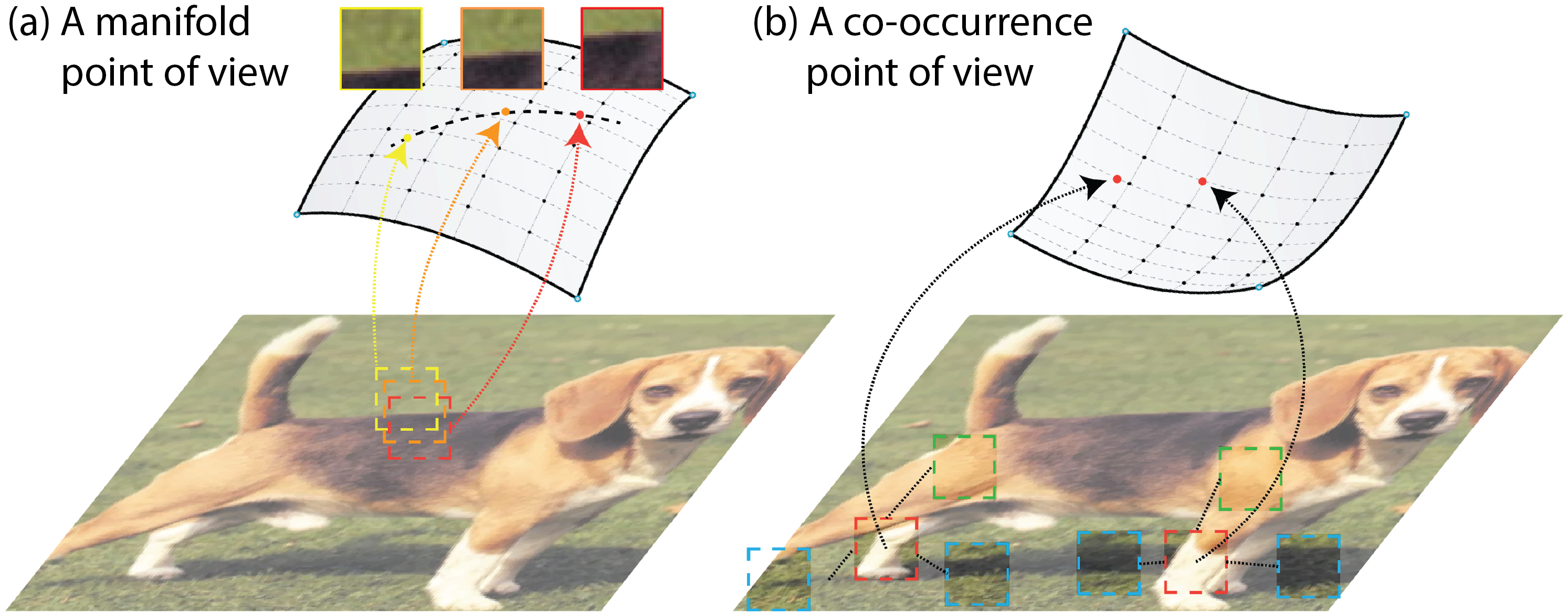
Figure 1: Two different points of view. (a) Manifold: There are three patches in the dashed boxes. Let’s assume there is a path between them on a manifold of the image patch space; then, their relationship can be found based on either the Euclidean neighborhoods, spatial co-occurrence, or temporal co-occurrence from smooth transformation. (b) Probabilistic: For the two red boxes (“leg”), it is unclear whether there is a path between them in the patch space. However, they can still be considered to be similar under spatial co-occurrence because they appear in the same context. These two patches both co-occur with the “grass land” (blue boxes) and “elbow or body” (green boxes). Temporal co-occurrence has a similar effect.

2 Unsupervised Learning with the Sparse Manifold Transform

The sparse manifold transform. The sparse manifold transform (SMT) was proposed to unify several fundamental unsupervised learning methods: sparse coding, manifold learning, and slow feature analysis. The basic idea of SMT is: 1) first to lift the raw signal $x$ into a high-dimensional space by a non-linear sparse feature function $f$, i.e. $\vec{\alpha}=f(\vec{x})$, where locality and decomposition are respected. 2) then to linearly embed the sparse feature $\vec{\alpha}$ into a low-dimensional space, i.e., find $\vec{\beta}=P\vec{\alpha}$, such that the similarity or “trajectory linearity”[21] is respected. As we mentioned earlier, for each data point $x_{i}$, we can choose to use either its local neighbors in the raw signal space, its spatial co-occurrence neighbors, or its temporal co-occurrence neighbors to define similarity. Let’s denote the neighbors of $\vec{x}_{i}$ as $\vec{x}_{n(i)}$, and denote $\vec{\alpha}_{i}$ as the sparse feature of $\vec{x}_{i}$. The optimization objective of finding similarity-preserving linear projection $P$ is the following:

$$\underset{P}{\text{min}}\,\sum_{i}\sum_{j\in n(i)}\|P{\vec{\alpha}_{i}}-P{\vec{\alpha}_{j}}\|_{F}^{2},\quad\text{s.t.}\quad P\ {\mathbb{E}}[\vec{\alpha}_{i}{\vec{\alpha}_{i}}^{T}]P^{T}=I$$ (1)

Example sparse feature extraction function $\vec{\alpha}=f(\cdot)$ could be sparse coding [82] and vector quantization [42], which will be further explained in Section 3.

Similarity can be considered as a first-order derivative (see Appendix L for detailed explaination). A more restrictive requirement is linearity [89], which is the second-order derivative. Then the objective is changed to a similar one:

$$\underset{P}{\text{min}}\,\sum_{i}\|P{\vec{\alpha}}_{i}-\sum_{j\in n(i)}w(i,j)P{\vec{\alpha}}_{j}\|_{F}^{2},\quad\text{s.t.}\quad P\ {\mathbb{E}}[\vec{\alpha}_{i}{\vec{\alpha}_{i}}^{T}]P^{T}=I$$ (2)

where $\sum_{j\in n(i)}w(i,j)=1$. Several ways to acquire $w(\cdot,\cdot)$ are: to use locally linear interpolation, temporal linear interpolation, or spatial neighbor linear interpolation. If we write the set $\{{\vec{\alpha}_{i}}\}$ as a matrix $A$, where each column of $A$ corresponds to the sparse feature of a data point, then both Optimization 1 and Optimization 2 can be formulated as the following general formulation [21]:

$$\underset{P}{\text{min}}\,\|PAD\|_{F}^{2},\quad\text{s.t.}\quad PVP^{T}=I$$ (3)

where $D$ is a differential operator, $V=\frac{1}{N}AA^{T}$ and $N$ is the total number of data point. $D$ corresponds to a first-order derivative operator in Optimization 1 and a second-order derivative operator in Optimization 2. For Optimization 1, $D$ has M columns, where $M$ denote the number of pair of neighbors. $D=[{\bf d_{1}},{\bf d_{2}},\cdots{\bf d_{M}}]$ and for $k^{th}$ pair of neighbors $x_{i},x_{j}$, we have ${\bf d_{k}}_{i}=1$ and ${\bf d_{k}}_{j}=-1$. All other elements of $D$ are zero. For Optimization 2, $D_{ji}=-w(i,j)$ for $j\in n(i)$, $D_{ii}=1$, and $D_{ji}=0$ otherwise. The solution to this generalized eigen-decomposition problem is given [109] by $P=UV^{-\frac{1}{2}}$, where $U$ is a matrix of $L$ trailing eigenvectors (i.e. eigenvectors with the smallest eigenvalues) of the matrix $Q=V^{-\frac{1}{2}}ADD^{T}A^{T}V^{-\frac{1}{2}}$. Please note that if $U$ contains all of the eigenvectors of $Q$, then the solution of SMT reduces to the whitening matrix.

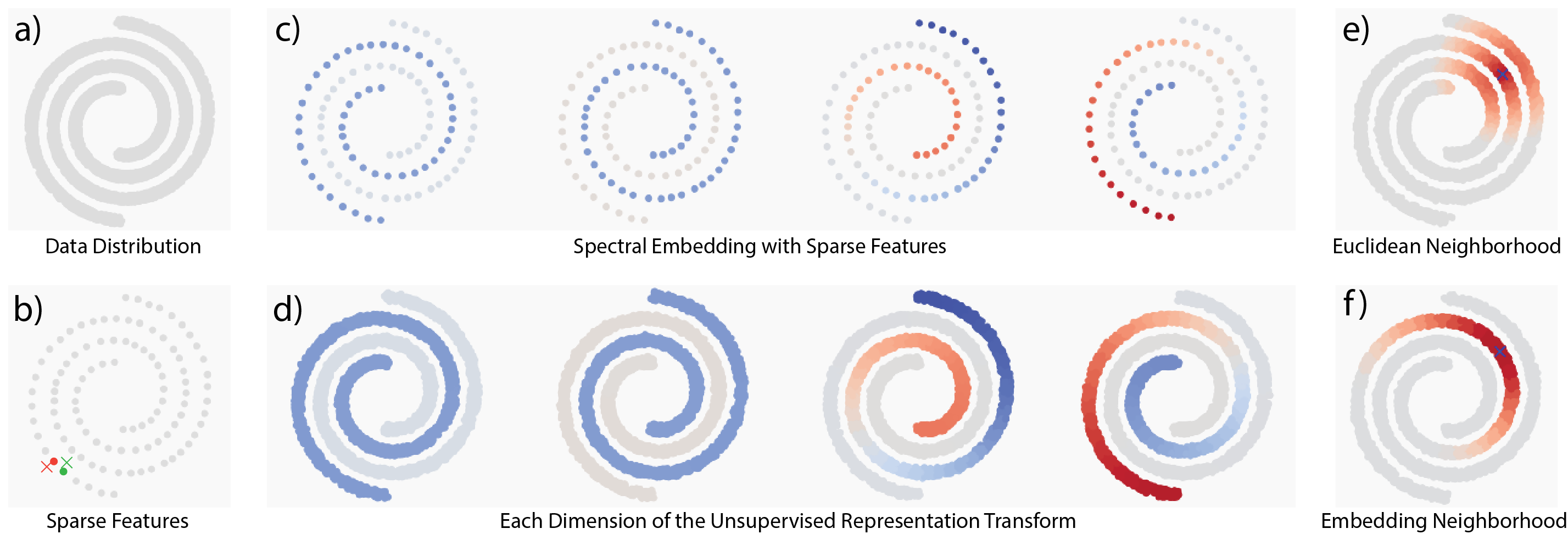
Figure 2: Manifold disentanglement with SMT. (a) Data distribution along two entangled 1D spiral manifolds in the 2D ambient space. (b) Sparse feature (dictionary) learned with 1-sparse sparse coding is shown as dots. They serve as a set of landmarks to tile the data manifolds. Given two points marked as red and green crosses, the 1-sparse feature function maps them to the corresponding dictionary element, marked as red and green dots. (c) Spectral embedding assigns similar values to nearby dictionary elements. Each embedding dimension is a low-frequency function defined on the sparse dictionary support. We show the first 4 embedding dimensions, i.e., the first 4 rows of $P$, $P_{1,\cdot}$, $P_{2,\cdot}$, $P_{3,\cdot}$, and $P_{4,\cdot}$. The color represents the projection values for each dictionary element. (d) The sparse manifold transform is a vector function $Pf(\cdot)$, and we plot the first four dimensions of SMT over the data distribution. The color represents the projection values for each data point. (e) We show the Euclidean neighborhood of the point marked by a blue cross in the original data space. (f) After the sparse manifold transform, we show the cosine similarity neighborhood of the point marked by the same blue cross in the representation space.

Manifold point of view: a 2D nonlinear manifold disentanglement problem. Let’s consider a spiral manifold disentanglement problem in a 2D space shown in Figure 2(a). As it is not a linearly-separable problem, to construct a representation function to disentangle the two spiral manifolds, we need to leverage nonlinearity and give the transform function enough flexibility. Let’s first use 1-sparse sparse coding to learn an overcomplete dictionary $\Phi\in\mathbb{R}^{2\times K}$ , i.e. a set of $K$ landmarks [98; 27], to tile the space. This dictionary serves as the support of the representation function, as shown in Figure  2(b). This dictionary turns a data point $\vec{x}$ into a 1-sparse vector $\vec{\alpha}=f(\vec{x})=\text{argmin}_{\vec{\alpha}}\|\vec{x}-\Phi\vec{\alpha}\|,\text{s.t.}\|\vec{\alpha}\|_{0}=1,\|\vec{\alpha}\|_{1}=1$; $\vec{\alpha}\in{\rm I\!R}^{K}$ is an 1-hot vector and denotes the closest dictionary element $\vec{\phi}$ to $\vec{x}$. Next, we seek a linear projection $P$ to embed the sparse vector $\vec{\alpha}$ to a lower dimensional space, $\vec{\beta}=Pf(\vec{x})$ and $\vec{\beta}\in{\rm I\!R}^{d}$, which completes the transform. Each column of $P\in{\rm I\!R}^{d\times K}$ corresponds to a $d$-dimensional vector assigned to the corresponding entry of $\alpha$. The $i^{th}$ row, $P_{i,\cdot}$, of $P$ is an embedding dimension, which should assign similar values to the nearby landmarks on the manifolds. As we mentioned earlier, there are three localities to serve as similarities, where they behave similarly in this case. With either of the three, one can define the Optimization 1 or Optimization 2. In this simple case, the different similarity definitions are almost identical, leading to a spectral solution of $P$. Let’s choose a simple construction [69]: given a data point $\vec{x}\in{\rm I\!R}^{2}$, add Gaussian noise $\epsilon_{1},\epsilon_{2}$ to it to generate two augmented samples $\vec{x}_{1}=x_{1}+\epsilon_{1}$ and $\vec{x}_{2}=x_{2}+\epsilon_{2}$, which are marked as the red and green crosses in Figure 2(b) and are considered as similar data points. $f(\vec{x}_{1})$ and $f(\vec{x}_{2})$ are marked as red and green dots (landmarks). So the objective in Optimization 1 is to find $P$ such that $\mathbb{E}_{x\sim p(x),\epsilon_{1},\epsilon_{2}\sim\mathcal{N}(0,I)}\|Pf(x_{1}+\epsilon_{1})-Pf(x_{2}+\epsilon_{2})\|^{2}$ is minimized. We show the solution in Figure 2(c) with the first four embedding dimensions, $\{P_{1,\cdot},P_{2,\cdot},P_{3,\cdot},P_{4,\cdot}\}$ plotted, where the color reflect their values at each dictionary element. As we can see, each embedding dimension, e.g. $P_{i,\cdot}$, is essentially a low-frequency function.  $P_{1,\cdot}$, $P_{2,\cdot}$ are piecewise constant functions on the union of the manifolds. Essentially, either $P_{1,\cdot}$ or $P_{2,\cdot}$ will suffice to determine which manifold a point belongs to. $P_{2,\cdot}$, $P_{3,\cdot}$ are non-constant linear functions along the manifolds. A linear combination of $P_{3,\cdot}$ and $P_{4,\cdot}$ will preserve the coordinate information of the manifolds. Now with both the sparse feature function $f$ and the spectral embedding $P$, we have constructed a sparse manifold transform, i.e. $\vec{\beta}=Pf(\vec{x})$. In Figure 2(d), we show how each dimension of this transform assigns different values to each point in the original 2D space, and the points from the same manifold are placed much closer in the representation space as shown in Figure 2(f).

Probabilistic point of view: co-occurrence modeling. Many related variations of spectral and matrix factorization methods have been widely used to build continuous word representations. SMT formulation bears a probabilistic point of view, which complements the manifold perspective. A notable example is the word co-occurrence problem. Here we present an SMT-word embedding. Given a corpus and a token dictionary, we can treat each token as a 1-hot vector $\vec{\alpha}$. Then we can seek a linear projection $P$ such that tokens co-occur within a certain size context window are linearly projected closer. After we solve Optimization 1, each column of $P$ corresponds to a continuous embedding of an element from the token dictionary. We train SMT on WikiText-103 [76] and provide the visualization result in Appendix A. As we discussed earlier, “Seattle” and “Dallas” may reach a similar embedding though they do not co-occur the most frequently. The probabilistic view of SMT explains the phenomenon that two embedding vectors can be close in the representation space if they frequently appear in similar contexts, though they may not be close in the signal space.

Sparsity, locality, compositionality, and hierarchy. (a) Sparsity: In the sparse manifold transform, sparsity mainly captures the locality and compositionality, which builds a support for the spectral embedding. Spectral embedding, on the other hand, would assign similar values to similar points on the support. (b) Locality: In a low-dimensional space, e.g., the 2D manifold disentanglement case, with enough landmarks, using 1-sparse feature $f_{vq}$ to capture locality will suffice, and SMT can directly solve the problem as we showed earlier. Please note that, in this simple case, this process is not different from manifold learning [89; 105] and spectral clustering [80]. One can also use a kernel, e.g. RBF kernel or the heat kernel, to respect locality by lifting to a higher or infinite dimensional space [95; 112; 6; 102; 8]. (c) Compositionality: If the signal comes from a high-dimensional space, e.g. images, then we may need to build the representation for image patches first since even local neighborhoods can become less reliable in high-dimensional space with finite samples. If the patch space is simple enough, e.g. MNIST, using 1-sparse vector quantization as the sparse feature $f_{vq}$ would be sufficient to capture the locality in patch space. As we will show later in Section 3, the SMT with 1-sparse feature $f_{vq}$ achieves over 99.3% top-1 KNN accuracy. For more complex natural images, e.g. CIFAR or ImageNet, compositionality exists even in the patch space. So 1-sparse feature becomes less efficient and may compromise the fidelity of the representation. As we will show, the general sparse feature will achieve better performance than the 1-sparse feature in this case.

(d) Hierarchy: For high-resolution images, we may need to stack several layers of transforms in order to handle the hierarchical representation [108; 35; 52].

SMT representation for natural images. We use SMT to build representation for image patches and aggregate patch representation of an image as the image representation. For an $S\times S$ image, we extract every $T\times T$ image patches as shown in Figure 3. Each of the image patches is whitened and L2-normalized, which resembles the early visual system processing [110; 74]. Given an image, we denote the pre-processed image patches as $\{\vec{x}_{ij}\}$, where $i$ indicates the vertical index of the patch and $j$ indicates the horizontal index. For each image patch $\{\vec{x}_{ij}\}$, we define its neighbors to be other patches within a certain pixel range from it on the same image, i.e., $n(ij)=\{\ lm;\ |i-l|\leq d\ \text{and}\ |j-m|\leq d\}$. Given a sparse feature function $f$, we would like to map these neighboring patches to be close in the representation space. If we choose $d=S-T+1$, then all the patches from the same image are treated as neighbors to each other. Given $f$, $d$, and a set of training images, we can calculate $ADD^{T}A^{T}$, $V$, and solve Optimization 1 for $P$. The representation of patch $\vec{x}_{ij}$ is $\vec{\beta}_{ij}=Pf(\vec{x}_{ij})$ with a L2 normalization. If we denote all of the patch representations from an image as tensor $B$, the image representation is $\vec{z}=\text{L2\_normalize\_pw}\left(\text{avg\_pool}(B;\text{ks},\text{stride})\right)$. $\text{avg\_pool}(\cdot;\text{ks},\text{stride})$ denotes the average pooling operator, where ks and stride are the kernel size and stride size of the pooling respectively. L2_normalize_pw denotes a point-wise L2 normalization. We use tensor $\vec{z}$ as a vector for an image representation. The detailed settings, e.g. $d,\text{ks},\text{stride}$, etc., are left to the experiments section. In this work, we primarily use the soft-KNN classifier to evaluate the quality of representation.

Connection to the deep latent-embedding methods. There are important connection between the SOTA latent-embedding SSL methods[18; 5]. In particular, Optimization 1 can be considered the simplest form of VICReg [5], whereas the VC regularization is replaced by a hard constraint, and a sparse feature function replaces the deep neural encoder. See exact formulation in Appendix K. This connection is even stronger given the evidence that VICReg is essentially building a representation of image patches [22]. In this sense, SMT can be considered the simplest form of VICReg.

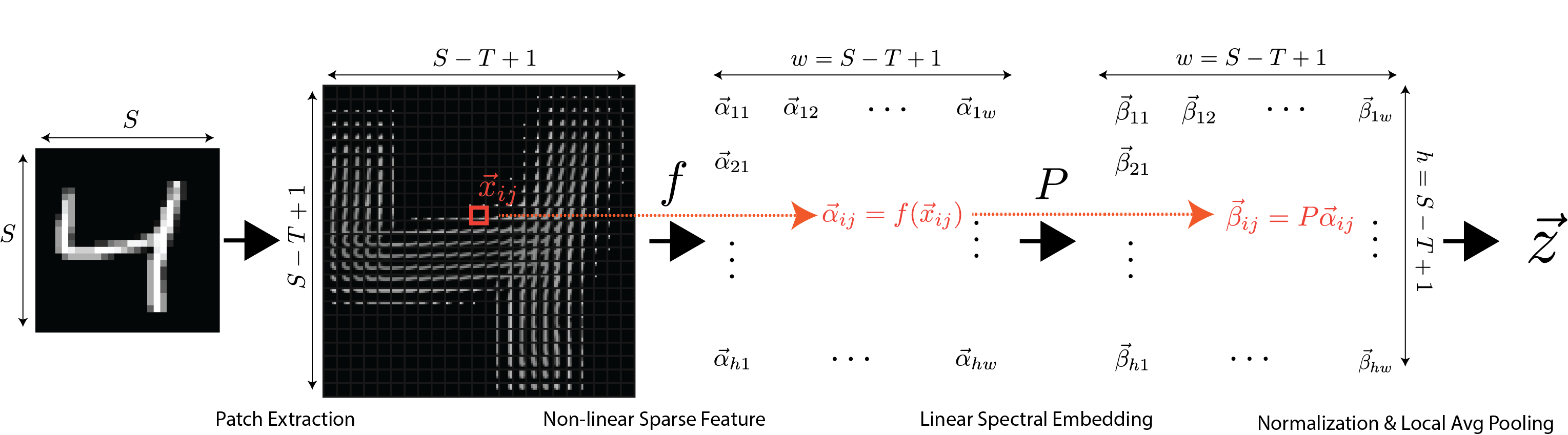
Figure 3: SMT representation of an image and its patches. An $S\times S$ image is first decomposed into $(S-T+1)\times(S-T+1)$ overlapping image patches of size $T\times T$. Each image patch is whitened and the sparse feature is calculated, $\vec{\alpha}_{ij}=f(\vec{x}_{ij})$, where $ij$ indicates the spatial index of the image patch and $\vec{x}_{ij}$ is the whitened patch. The representation of patch $\vec{x}_{ij}$ is $\vec{\beta}_{ij}=Pf(\vec{x}_{ij})$ with a L2 normalization. We then aggregate these patch representations $\vec{\beta}_{ij}$ via spatial local average pooling and L2-normalize at every spatial location to obtain the final image-level representation $\vec{z}$.

3 Empirical Results

In this section, we first provide the benchmark results on MNIST, CIFAR-10, and CIFAR-100. Qualitative visualization is also provided for a better understanding. We also compare 1-sparse feature $f_{vq}$ and a more general sparse feature $f_{gq}$. $\vec{\alpha}=f_{vq}(\vec{x};D)$ refers to the 1-sparse vector quantization sparse feature, where $\vec{\alpha}_{i}=1$ for $i=\text{argmax}_{i}\|\vec{x}-D_{\cdot,i}\|_{2}$ and $D$ is a dictionary. We denote the SMT representation with $f_{vq}$ sparse feature as SMT-VQ. $\vec{\alpha}=f_{gq}(\vec{x};D,t)$ refers to a more general sparse function, where each column of dictionary $D$ is an image patch and $t$ is a given threshold. For $\vec{\alpha}=f_{gq}(\vec{x};D,t)$, the $i$th entry of $\vec{\alpha}$ is $1$ if only if the cosine similarity between $\vec{x}$ and $i$th dictionary element pass the threshold, i.e., $\alpha_{i}=1$ if $cos(\vec{x},D_{\cdot,i})\geq t$ and $\alpha_{i}=0$ otherwise. We denote the SMT representation with $f_{gq}$ feature as SMT-GQ. We find $f_{gq}$ achieves similar performance as the sparse coding feature in benchmarks, and it’s more efficient in experiments since it does not involve a loopy inference. For both MNIST and CIFAR, we use 6x6 image patches, i.e., $T=6$. All the image patches are whitened, and the whitening transform is described in Appendix C. Once patch embeddings are computed, we use a spatial average pooling layer with $\text{ks}=4$ and $\text{stride}=2$ to aggregate patch embeddings to compute the final image-level embeddings.

MNIST. For MNIST, 1-sparse feature $f_{vq}$ is sufficient to build good support of the patch space. The dictionary $D\in{\rm I\!R}^{36\times K}$ is learned through 1-sparse sparse coding, which is equivalent to clustering and can be implemented with any clustering algorithm. The centroid of each cluster will serve as a dictionary element. The detailed learning procedure is left to Appendix D. The inference is equivalent to vector quantization. We chose the patch embedding dimension as 32 because further increasing the dimension does not improve the performance. In Table 1, we compare different dictionary sizes and different spatial co-occurrence ranges. We also compare the SMT embedding with the GloVe embedding. Treating each image patch as a token and the entire image patch as a sentence, we can train a GloVe word embedding model on MNIST patches. We provide a GloVe embedding with optimized settings. As we can see in Table 1, GloVe embedding works slightly worse in this case, even with a large dictionary size. Further, we can find that a small context range works slightly better for MNIST. This is probably due to the fact that the patch space of MNIST is closer to a manifold, and co-occurrence is less informative in this case. To further verify this hypothesis, we provide an ablation study on embedding dimensions in Table 2. Even if we reduce the embedding dimension to 4 , the top-1 KNN accuracy is still $98.8\%$. This implies that the MNIST patch space might be close to a manifold like high-contrast natural image patches [67; 26; 12].

Table 1: Evaluation of SMT representation on MNIST. The table shows the evaluation result of SMT embedding and GloVe embedding using a KNN classifier. We compare different dictionary size: 16384 vs. 65536 and context range: 3-Pixel ($d=3$) vs. Whole Image ($d=28-6+1$). We use 32 as the embedding dimension. As shown in the table, GloVe embedding works slightly worse than SMT embedding.

Co-Occurrence Context Range	SMT-VQ (16384)	SMT-VQ (65536)	SMT-VQ (GloVe, 100K)
Whole Image	99.0%	98.9%	98.8%
3 Pixels	99.2%	99.3%	99.0%

Table 2: Low dimensionality of MNIST patch space. The table shows the effect of the embedding dimension of SMT on the KNN evaluation accuracy. With only a 4-dimensional embedding for each patch, SMT can still achieve 98.8% KNN accuracy. The quick accuracy drop at 3-dimensional embedding space may imply that the MNIST patch space can be approximately viewed as a 3-manifold since the 4-dimensional patch embedding is L2-normalized and on a 3-sphere.

	Emb Dim=2	Emb Dim=3	Emb Dim=4	Emb Dim=8	Emb Dim=16	Emb Dim=32
KNN Acc	97.1%	98.3%	98.8%	99.0%	99.1%	99.2%

CIFAR-10 and CIFAR-100. For the CIFAR benchmarks, we compare both $f_{vq}(\cdot;D)$ and $f_{gq}(\cdot;D,t)$. The dictionary $D$ used in $f_{vq}$ is learned through 1-sparse sparse coding, and the dictionary $D$ used in $f_{gq}$ is just randomly sampled from all image patches for efficiency purposes. Since $f_{vq}$ with color patches underperforms that with grayscale patches, we choose to experiment mostly with $f_{gq}$ on CIFAR benchmarks. For $f_{gq}$, $t$ is set to $0.3$ with color patches and $0.45$ with grayscale patches. We choose the patch embedding dimension as 384. Further, with color patches, dropping the first $16$ embedding dimensions of $P$ improves the accuracy by about 1%. We compare the performance of SMT with SOTA SSL models, specifically, SimCLR and VICReg with a ResNet 18 backbone. We train these SSL models using random resized crop and random horizontal flip as default data augmentations. For a fair comparison, SMT training uses both the original version and the horizontally flipped version of the training set. We also experiment with different color augmentation schemes. For “Grayscale Image Only”, we train both SMT and SSL models using only grayscale images. For “Original + Grayscale”, we train SMT on both color images and grayscale images, then concatenates the embedding of each color image with the embedding of its grayscale version. We train SSL models with additional “random grayscale” color augmentations. With a two-layer deterministic construction using only image patches, SMT significantly outperforms SimCLR and VICReg, with no color augmentation. With “Grayscale Image Only” color augmentation, SMT-GQ achieves similar performance as SimCLR and VICReg. With “Original + Grayscale” augmentation, SMT-GQ performs on par with SimCLR and VICReg without colorjitter and several additional color augmentations. With full data augmentation, SimCLR and VICReg outperform SMT-GQ. However, we did not find a straightforward way to add these color augmentations to SMT-GQ. We can observe the same trend on CIFAR-100. Interestingly, SMT-GQ always significantly outperforms SimCLR and VICReg before we add color jittering and additional data augmentations. We provide further ablation studies in Appendix. Appendix G and Appendix H study how context range and the number of training samples affect the model performance. Appendix I studies different evaluation schemes (KNN vs. linear probing). Appendix E shows that the performance of SMT will significantly degrade if we replace spectral embedding with other dimension reduction algorithms that do not respect locality.

Table 3: Evaluation of SMT and SSL pretrained model on CIFAR-10. The table shows the evaluation result of SMT embedding and SSL pretrained models using KNN classifiers. We evaluated these models using various color augmentation schemes. The details of how we add color augmentation to each model are explained in section 3. We tried two sparse features for SMT: $f_{vq}$ and $f_{gq}$. For $f_{gq}$, we tried two dictionary sizes: 8192 and 65536. Both SSL models use ResNet-18 as a backbone and are optimized for 1000 epochs through backpropagation; SMT uses a 2-layer architecture and is analytically solved, which can be considered as 1 epoch.

Color Augmentation	SMT-VQ (100K)	SMT-GQ (8192)	SMT-GQ (65536)	SimCLR (ResNet18)	VICReg (ResNet18)
Original Image	—	79.2%	81.1%	68.3%	70.2%
Grayscale Image Only	78.4%	77.5%	78.9%	80.6%	81.3%
Original + Grayscale	—	81.4%	83.2%	85.7%	83.7%
Full (ColorJitter etc.)	—	—	—	90.1%	91.1%

Table 4: Evaluation of SMT and SSL pretrained model on CIFAR-100. The table shows the performance of SMT embedding and two other SSL pretraining methods on the CIFAR-100 dataset. The data augmentation and different SMT variations we used in this experiment are the same as those for evaluating CIFAR-10 dataset in Table 3. For CIFAR-100 dataset, without full color augmentation, SMT always outperforms the two SSL pretraining methods.

Color Augmentation	SMT-VQ (100K)	SMT-GQ (8192)	SMT-GQ (65536)	SimCLR (ResNet18)	VICReg (ResNet18)
Original Image	—	50.8%	53.2%	32.4%	32.6%
Grayscale Image	46.6%	45.8%	48.9%	43.0%	43.9%
Original + Grayscale	—	53.7%	57.0%	48.9%	46.0%
Full (ColorJitter etc.)	—	—	—	63.7%	65.4%

Visualization. For a better understanding, we provide a visualization of the patch embedding space with the 1-sparse feature in Figure 4. Given a dictionary $D$, each dictionary element is an image patch in the whitened space. For a dictionary element shown in the red box, we can visualize its nearest neighbors, measured by cosine similarity, in the embedding space. All the image patches are unwhitened before visualization, where the detail is left to the Appendix C. In Figure 4, we can see that the nearest neighbors are all semantically similar. a) is a slightly curved stroke of a digit in MNIST. b) shows the patch of the center of a digit “4”. c) shows a part of a “wheel” of a car in CIFAR. d) shows a part of “animal face”. These results are similar to the 2D results shown in Figure 2. Overall, the representation transform brings similar points in the data space closer in the representation space. Additional visualization for SMT on CIFAR-10 dataset is in Appendix M.

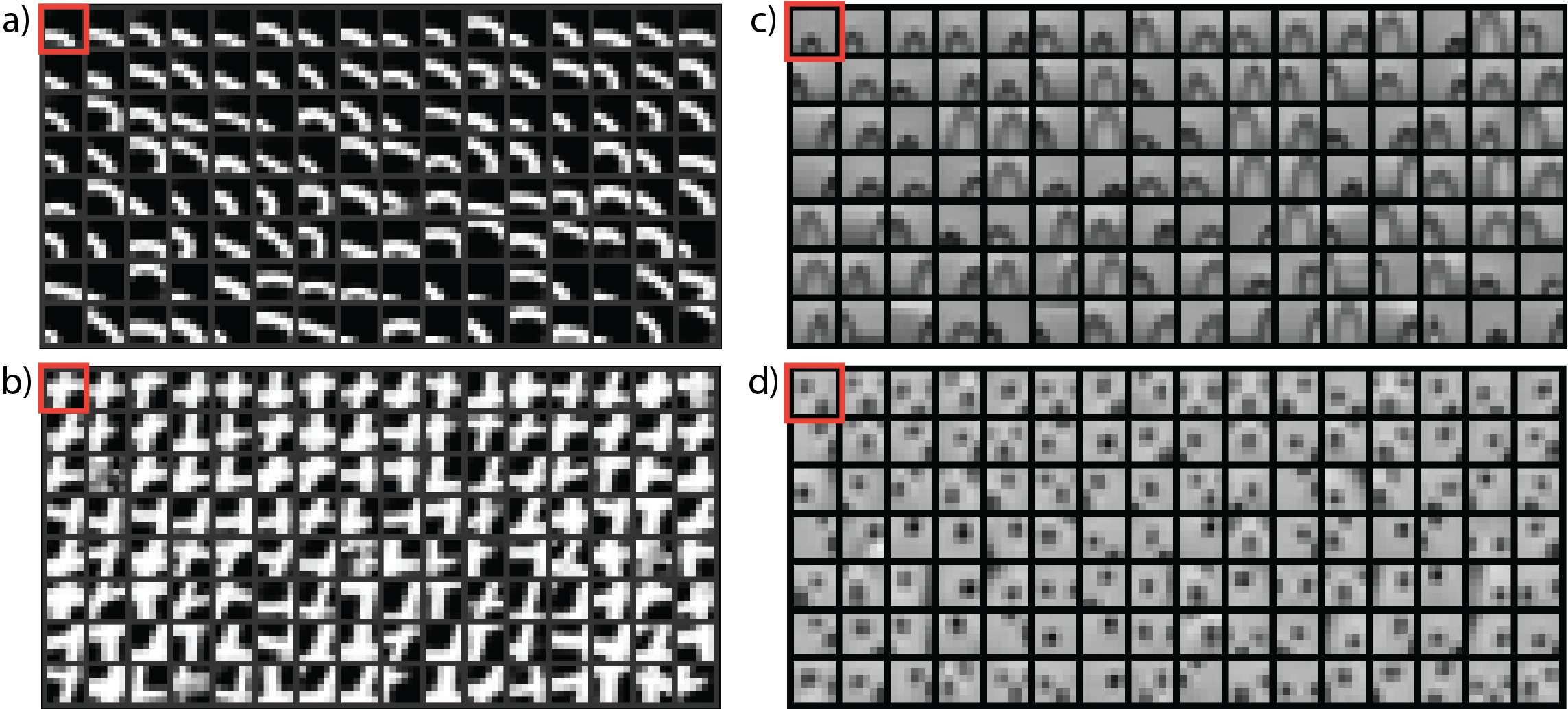
Figure 4: Visualization of dictionary elements’ neighborhoods in the SMT embedding space. We plot 4 different dictionary element and their top nearest neighbors in four subfigures, respectively. For each subfigure, the dictionary element is shown in the red box. Its neighboring patches in the representation space are ordered by their cosine similarity to the dictionary element, where the image patches in the top left have highest cosine similarity, and image patches on the bottom right have lowest cosine similarity. This figure is qualitatively similar to Figure 2(f) except it is in a high-dimensional space and the semantic meaning is more complex.

4 More Related Works

There are several intertwined quests closely related to this work. Here, we touch them briefly.

The state-of-the-art unsupervised methods. Deep learning [63; 66] is the engine behind the recent revolution of AI. Given the right craftsmanship, deep neural networks are powerful optimization tools to allow us express various engineering objectives conveniently. It has also revolutionized the unsupervised visual representation learning in the past few years [113; 47; 18; 5]. Understanding the engineering advancements can help us gain deeper theoretical insights and many efforts have been made [85; 1; 70; 2; 94] towards this goal.

To model the patterns of the signal spaces. A central challenge of modeling the signals is the formalization of a small set of ideas for constructing the representations of the patterns[43; 79]. Wavelet transform[72; 24] was formulated to handle the sparsity in the natural signals. Steerable and shiftable filters[38; 101; 99] were introduced to handle the discontinuity of wavelet filters with respect to the natural transformations. Basis pursuit[17; 16] finds decomposition of a signal by a predefined dictionary, sparse coding[81; 82], and ICA[7; 56] were proposed to learn the filters or dictionary from data. Before the sparse manifold transform[21], many important works have paved the way and introduced topology and transformations between the dictionary elements[57; 58; 11]. There are also several important works studying the natural image patch space with non-parametric methods and topological tools [67; 26; 12; 48]. Manifold learning[89; 105; 44] and spectral clustering [33; 37; 95; 75; 80; 104; 93] was proposed to model the geometric structure in the signal space. The geometric signal processing is also an increasingly important topic[96].

Modeling of biological visual system. Exploring the geometric or statistical structure of natural signals are also strongly motivated by computational modeling of biological visual system. Many properties of the visual system reflect the structure of natural images [100; 59]. An early success of this quest was that the dictionary elements learned in an unsupervised fashion closely resemble the receptive fields of simple cells in the V1 cortex[81; 82]. In order to further understand the visual cortex, we need to develop theories that can help to elucidate how the cortex performs the computationally challenging problems of vision [83]. One important proposal is that the visual cortex performs hierarchical manifold disentanglement [31; 32]. The sparse manifold transform was formulated to solve this problem, which is supported by a recent perceptual and neuroscience evidence [49; 50]. There are also several related seminal works on video linearization [112; 41; 40].

To build representation models from the first principles. The now classical models before deep learning use to be relatively simpler [64; 108; 87; 60; 111; 115; 61], where sparsity was a widely adopted principle. While the gap between the SOTA deep learning models and the simple models is large, it might be smaller than many expect [23; 88; 10; 106]. The quest to build “white-box” models from the first principles [14; 13; 71] for unsupervised representation remains an open problem.

5 Discussion

In this paper, we utilize the classical unsupervised learning principles of sparsity and low-rank spectral embedding to build a minimalistic unsupervised representation with the sparse manifold transform [21]. The constructed “white-box” model achieves non-trivial performance on several benchmarks. Along the way, we address fundamental questions and provide two complementary points of view of the proposed model: manifold disentanglement and co-occurrence modeling. Further, the proposed method has close connections with VICReg [5] and several other SOTA latent-embedding SSL models [18; 117; 39]. However, there are several important limits to this work, which point to potential future directions. 1) We need to scale the method to larger datasets, such as ImageNet. 2) While a two-layer network achieves non-trivial performance, we need to further construct white-box hierarchical models to understand how a hierarchical representation is formed [51; 53]. 3) While spectral embedding is context-independent [86; 118], there is clear benefit in building contextualized embedding [29; 91; 52; 36; 116; 73]. Building a minimalistic unsupervised representation based on contextualized embedding is an attractive topic for additional research. 4) Although we only focus on sparse feature in this paper, other features should also be explored. We can generalize feature extraction function $f$ in SMT to an arbitrary function as long as it can capture the locality and structures in the signal space. For example, if we choose $f$ as a quadratic expansion function, Optimization 1 would reduce to slow feature analysis [112].

The evidence shows that there considerable promise in building minimalistic white-box unsupervised representation learning models. Further reducing the gap with SOTA methods and understanding the mechanism behind this reduction can lead us towards a theory. Minimalistic engineering models are easier to analyze and help us build a theory to identify optimality and efficiency, and a testable theory can also facilitate modeling biological learning systems. This work takes a step towards these goals.

Acknowledgments

We thank Zengyi Li, Jamie Simon, Sam Buchanan, Juexiao Zhang, Christian Shewmake, Jiachen Zhu, Domas Buracas, and Shengbang Tong for participating in several intriguing discussions during the preparation of this manuscript. We also thank Fritz Sommer and Eero Simoncelli for providing valuable feedback. We also thank our anonymous reviewers for the helpful suggestions and insightful questions, which helped us improve the manuscript considerably.

Appendix

Appendix A Probabilistic point of view example: SMT word embedding

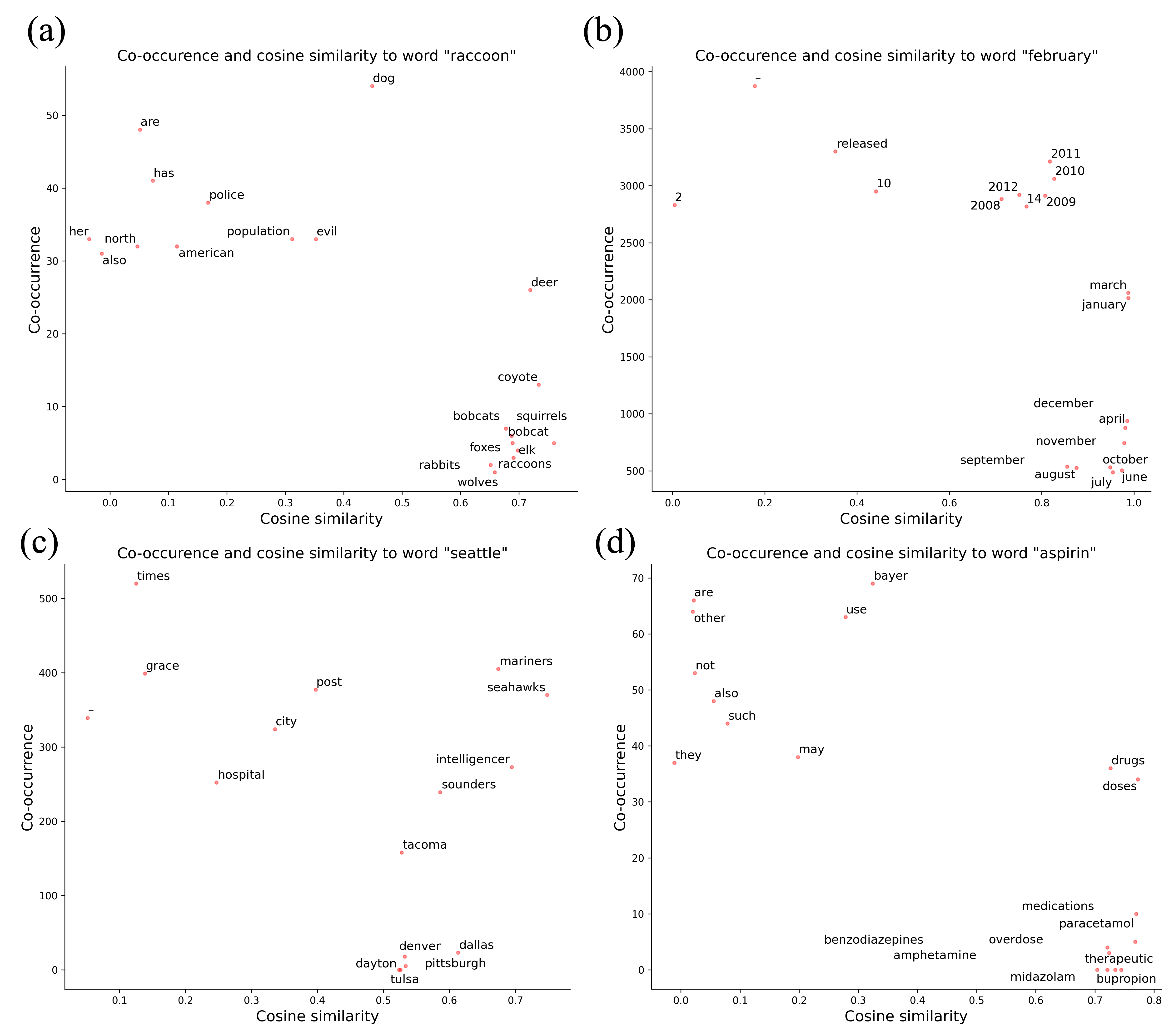
Figure 5: Visualization of SMT word embedding. For each word “raccoon”, “February”, “Seattle” and “aspirin”, we plot the top 10 words that are closest to it in the embedding space, and we show the top 10 words that co-occur with it the most. Two words are close if the cosine similarity between their SMT embedding is high. The co-occurrence is calculated based on the entire corpus. We count two words that co-occurred once if they appear in the same context window. The co-occurrence is plotted against the cosine similarity.

We use SMT to build word embedding for the vocabulary in WikiText-103 to illustrate the probabilistic view of SMT. Unlike in Figure 2, where the neighbor of each data point $x$ can be interpreted as its Euclidean neighborhood, there is no such distance function in the natural language. Nevertheless, we could still define neighborhood for each word. We define the neighbor of each word as other words that co-occur with it in a given context.

Like the manifold learning view, where the global geometry emerges despite only local neighborhoods being used during training, such a phenomenon is also observed from the probabilistic point of view. To visualize this phenomenon from a probabilistic point of view, we measure the co-occurrence of each pair of words and the cosine similarity between them in their SMT embedding space. In figure 5 (a), we show the top 10 words that are closest to “raccoon” and the top 10 words that co-occur the most with “raccoon”. We can see words like “American,” and “population” co-occur with “raccoon” a lot, but neither “American” nor “population” are close to “raccoon” in the embedding space. Instead, words that are semantically related to “raccoon” are close to “raccoon” in the embedding space, like “squirrels”, “rabbits” and “wolves”, even though they rarely co-occur with “raccoon.” The underlying reason is that these words share the same context patterns as “raccoon”. Although words like “American” and “population” can co-occur with “raccoon” in phrases like ”American raccoon” and ”raccoon’s population,” these words also co-occur with other words in very different contexts. Thus, they could not be embedded to be close “raccoon.”

We also illustrate three more examples in figure 5. In (b), we see words that occur with “February” are other months like ”July,” ”June,” and ”September.” In (c), words co-occur with “Seattle” the most are other large cities like “Dallas”, “Denver” and “Pittsburgh”, even though they rarely occur with “Seattle.” Finally, in (d), the words co-occur with “aspirin” the most are names of other medicines.

Appendix B Details for training word embedding using SMT

Dataset. We use WikiText-103 corpus [76] to train SMT word embedding, which contains around 103 million tokens. We use “Basic English Tokenizer” from torchtext, which uses minimal text normalization for the tokenizer. We tokenize and lowercase the WikiText-103 corpus, building a vocabulary using the top 33,474 words with the highest frequency. Notice that this dataset is significantly smaller than the Wikipedia dump used to train GLoVe in the original paper [86]. Wikipedia is also highly biased toward technical subjects, which is reflected in our word embedding.

SMT training. First, we choose the one-hot encoding as the sparse extraction function $f$. Each token in the text corpus is considered a data point $\vec{x_{i}}$; it is first transformed into a one-hot vector by $f$, then encoded to be close to its neighbor via spectral embedding. In order to perform spectral embedding, we need to define the neighbor(context) for each word in Optimization 1. In this case, each word’s neighbor(context) is its previous four words and the next four words. We can then calculate $ADD^{T}A^{T}$, $V$, and solve Optimization 1 for $P$. The representation of each word in the vocabulary is simply each column of P. This is because $f$ is one-hot encoding, for each word $\vec{x_{i}}$, we have $\vec{\beta_{i}}=Pf(\vec{x_{i}})=P{\bf e_{i}}=\vec{P_{i}}$.

Appendix C Whitening of the image patches

We consider all the square image patches with size $T\times T\times c$, where $T$ is patch size, and $c$ is channel size, as flattened vectors of dimension $T^{2}c$. We first remove the mean from each patch. Instead of calculating the global mean like in the normal whitening procedure, we calculate the contextual mean. Let $x_{i}$ denote a image patch and let $N_{i}=\{x_{j}:j\in n(i)\}$ denote the neighboring patch for $x_{i}$. We can calculate the contextual mean of $x_{i}$ as $\mu_{i}=\frac{1}{||N_{i}||}\sum_{j\in N_{i}}x_{j}$. Let $\bar{x_{i}}$ denote the mean removed image patch, then $\bar{x_{i}}=x_{i}-\mu_{i}$. We could also simply calculate the global mean $\mu$ and use it to center all the image patches. However, we found using contextual mean improve performance.

We apply the whitening operator to the mean-removed image patches. Let $\{\vec{x}_{i}\}$ denote the pre-processed image patches. Then we have

$$\vec{x}_{i}=(\lambda I+\Sigma)^{-\frac{1}{2}}\bar{x_{i}}$$

To “unwhiten” the patch for visualization, we multiply the whitened patch with the inverse of whiten operator: $(\lambda I+\Sigma)^{\frac{1}{2}}$.

Appendix D 1-Sparse Dictionary Learning

Given $\vec{x_{i}}\in\mathbb{R}^{d}$ to be a data vector, and dictionary (codebook) $\Phi\in\mathbb{R}^{d\times K}$, where $d$ is the dimension of the data and $K$ is the number of dictionary elements, 1-Sparse Dictionary Learning, also known as Vector Quantization (VQ problem [42]), can be formulated as:

$$\begin{split}\min_{\vec{\alpha_{i}},\Phi}\sum_{i}||\vec{x}_{i}-\Phi\vec{\alpha}_{i}||_{2},\\ s.t.\quad||\vec{\alpha}_{i}||_{0}=1,||\vec{\alpha}_{i}||_{1}=1,\vec{\alpha}_{i}\succeq 0.\end{split}$$ (4)

This is an NP-hard problem, but there are efficient heuristic algorithms to approximate the solution. The most well-known one is K-mean clustering, which can be interpreted as an expectation-maximization (EM) algorithm for mixtures of Gaussian distributions. This is the algorithm we used to solve 1-sparse dictionary learning when we use the 1-sparse feature $f_{vq}$ in SMT. The exact algorithm we used to solve the 1-sparse dictionary learning problem is in Algorithm 1. Notice that when data is uniformly distributed on the domain, even a dictionary consisting of uniformly sampled data point serve as a good enough approximation. This is the case for the toy example in Figure 2. In this case, the dictionary $\Phi$ can be predefined instead of learned. For MNIST and CIFAR-10 data, they are both assumed to be low dimensional data manifolds in high dimensional space. Thus, we cannot apply k-mean directly to the raw signal due to the high dimensionality and sparsity of the data. One way to alleviate this problem is to map the data to a unit sphere before applying k-mean. This method is called spherical k-mean. More detailed motivations and advantages of this approach are explained in the original paper [30]. The exact algorithm is also described in Algorithm 1.

Data: Data matrix $X=[\vec{x}_{1},\cdots,\vec{x}_{N}]$, $\eta$ is learning rate.

Result: Dictionary (centroid) $\Phi=[\vec{\phi}_{1},\cdots,\vec{\phi}_{K}]$, where each column is a dictionary element

     Sparse code (label) $A=[\vec{\alpha}_{1},\cdots,\vec{\alpha}_{N}]$ for each data point.

1 initialization: $\Phi\leftarrow 0,A\leftarrow 0$ ;

2 if spherical then

3       for  $i\in 1,\cdots,n$  do

4             $\vec{x}_{i}=\frac{\vec{x}_{i}}{||\vec{x}_{i}||_{2}}$

5       end for

6      

7 end if

8while not $\phi$ has not converge do

9       Find the sparse code for every data point;

10       for  $i\in 1,\cdots,n$  do

11            $\vec{\alpha_{i}}\leftarrow\vec{e}_{j^{*}}\quad j^{*}=\operatorname*{arg\,max}_{j}||\vec{\phi}_{j}-\vec{x}_{i}||_{2}$

12       end for

13      Dictionary update;

14       $\Phi\leftarrow\Phi+\frac{\eta}{\vec{h}}\odot\sum_{i}(\vec{x}_{i}-\Phi^{T}\vec{\alpha}_{i}),\quad s.t.\quad\vec{h}_{j}=(\sum_{i}\vec{\alpha}_{i})_{j}$;

15       if spherical then

16             for  $j\in 1,\cdots,K$  do

17                   $\vec{\phi}_{j}=\frac{\vec{\phi}_{j}}{||\vec{\phi}_{j}||_{2}}$

18             end for

19            

20       end if

21      

22 end while

Algorithm 1 Online 1-sparse dictionary learning heuristic (K-mean clustering)

Appendix E Ablation study: feature dimension and embedding dimension

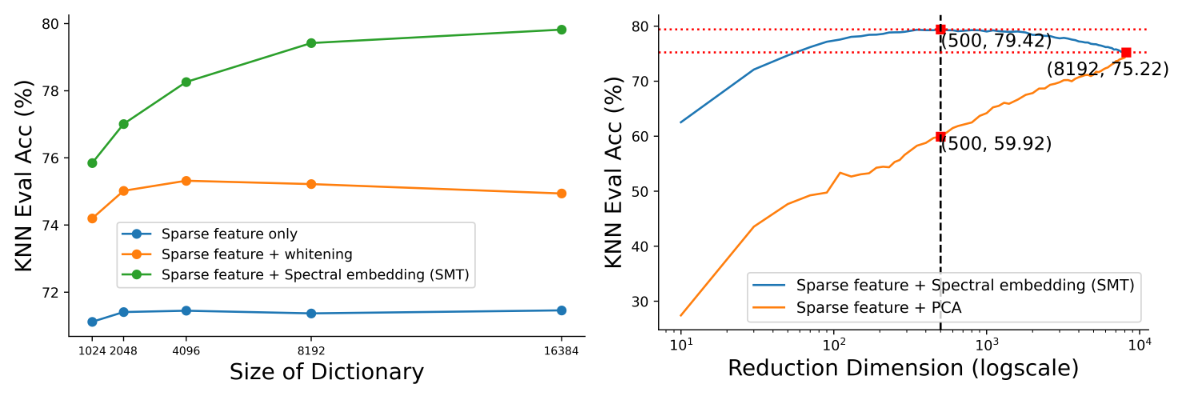
Figure 6: Ablation Studies. (a) Evaluation accuracy as a function of dictionary sizes on CIFAR-10 dataset. We tried three representations for ablation study purpose. (b) Evaluation accuracy as a function of reduction dimension on CIFAR-10 dataset. Reduction dimension corresponds to number of principle components in PCA and embedding dimension in SMT. We use general sparse feature $f_{gq}$ with threshold set to be $0.3$, a dictionary of size 8192 and no color augmentation in this experiment.

Since SMT is a white box model, we can analyze how each component of SMT contributes to unsupervised learning. Specifically, we break down SMT into two components: dimensionality expansion using sparse features and dimensionality reduction through spectral embedding. We first show that a sparse feature by itself is important in building a good representation. As shown in Figure 6, we’re able to achieve 71 % evaluation accuracy using only general sparse features $f_{gq}$ on the CIFAR-10 dataset. Please refer to Section 3 for the definition of general sparse features $f_{gq}$. Combining sparse features with whitening will further boost the performance to 75 %. However, the performance does not increase as the number of features increases if we’re using only sparse features and whitening. In contrast, if we combine sparse features and spectral embedding, the performance increases as the number of features increases. This result implies that spectral embedding is also a crucial element in obtaining a good representation.

To further show the necessity of spectral embedding, we did an experiment to replace spectral embedding with PCA. PCA is a dimension reduction algorithm but does not enforce locality. In Figure 6(b), we see that if we’re using PCA as dimension reduction, the performance decreases monotonically as we reduce the sparse feature to a lower dimension, which implies it is throwing away useful information. On the other hand, for SMT, the performance first increases and then decreases, as we increase the reduction dimension. The performance of SMT peaks when we use 500 as the reduction dimension, which is much higher than PCA (79.4% vs 59.9%) with 500 components and even higher than PCA with all principle components (79.4% vs 75.2%).

Appendix F Hyperparameter for pretraining deep SSL model

For all the benchmark results on the deep SSL model, we follow the pretraining procedure used in solo-learn. Each method is pretrained for 1000 epochs. We list the hyperparameter we used to pretrain each model. For both methods, we use resnet-18 as the backbone, and a batch size of 256, LARS optimizer, with 10 epochs of warmup follows by a cosine decay. For the SimCLR model, we set the learning rate to be 0.4 and a weight decay of 1e-5. We also set the temperature to 0.2, the dimension for the projection output layer to 256, and the dimension of the projection hidden layer to 2048. For VICReg, we set the learning rate to 0.3 and a weight decay of 1e-4. We also set the temperature to 0.2, and set the dimension for the projection output and hidden layer to 2048. We set the weight for similarity loss and variance loss to 25, and the weight for covariance loss to 1.

We use the transform module in pytorchvision to implement data augmentations. By default, we use “RandomResizedCrop” with min-scale equal to 0.08 and max-scale equal to 1.0. We also use “RandomHorizontalFlip” and use 0.5 as the flip probability. For “Grayscale Image Only”, we apply the “RandomGrayscale” transform with the grayscale probability to 1. For “Original + Grayscale,” we set the grayscale probability to 0.5. For “Full” color data augmentation, we add “ColorJitter.” For SimCLR, we use brightness = 0.8, contrast= 0.8, saturation=0.8, and hue=0.2 as its “ColorJitter” parameter. For VICReg, we use brightness = 0.4, contrast= 0.4, saturation=0.2, hue=0.1 as its “ColorJitter” parameter. We also add additional “Solarization” transform with probability 0.1 for training VICReg.

Appendix G Ablation study: context range

Given an image patch $\{\vec{x}_{ij}\}$, we define its neighbors to be other patches within a specific pixel range from it on the same image, i.e., $n(ij)=\{\ lm;\ |i-l|\leq d\ \text{and}\ |j-m|\leq d\}$. We use $d$ to denote the “context range”. We showed the impact of context range on MNIST in table 1. The performance of SMT decreases as we increase the context length. We also studied the effect of context length on the CIFAR-10 dataset and showed the result in table 5. Unlike MNIST, the performance on CIFAR-10 dataset increases as the context window increases. This once again confirms that both the manifold view and the probabilistic co-occurrence view are necessary to understand SMT. For CIFAR-10, the images have lots of high-level structures. The key to building a good representation is the ability to model the co-occurrence between different image patches. For example, in an image of an animal, the animal’s “leg” and “head” might lie in two image patches far apart. But it is very important to capture the fact that “leg” and “head” co-occur, because this is a unique trait for animals, which requires the context range to be large. This also requires the probabilistic co-occurrence view. Many image patches can be neighbors (co-occur), but they cannot all be encoded to the same point. Instead, if we record the co-occurrence, patches that co-occur more often should be encoded closer than to each other. On the other hand, MNIST is closer to a manifold, so co-occurrence is less informative in this case. Modeling co-occurrence between image patches might result in overfitting. In order to form a good representation, we need to use a small context range to capture slow features. This is a lot like the formulation in the original sparse manifold paper, where they use consecutive video frames to define context, which is essentially a context range of only 2 pixels.

Table 5: Ablation study on the context range used in SMT on CIFAR-10 dataset. We use general sparse feature $f_{gq}$ with threshold set to be $0.3$, a dictionary of size 8192 and no color augmentation in this experiment.

Context Range ($d$)	4	6	12	24	32
KNN Accuracy	78.0 %	78.5 %	78.5 %	79.0 %	79.4%

Appendix H Ablation Study: number of training examples

We experiment with the impact of a number of training examples on performance. The experiment is done on the CIFAR10 dataset. The result is shown in table 6. The result shows SimCLR experienced a much more significant performance drop compared to SMT when training with a limited amount of data. The significant performance drop of the deep SSL method is likely due to the well-known overfitting problem of complicated models like neural networks. This shows the advantages of SMT as a simple white-box model.

Table 6: Ablation study on the number of training examples used in SMT and SimCLR on CIFAR-10 dataset. We use general sparse feature $f_{gq}$ with threshold set to be $0.3$, a dictionary of size 8192 and no color augmentation in this experiment. We evaluate both method using soft KNN classifier.

number of training examples	1000	2000	4000	8000	16000	32000	50000
SMT-GQ (8192, no color aug)	58.7 %	63.7 %	67.2 %	70.7 %	74.0 %	77.4 %	79.4 %
SimCLR (ResNet18, no color aug)	28.9 %	33.9 %	37.8 %	41.3 %	50.1 %	60.4 %	68.3 %

Appendix I Ablation study: linear probing vs KNN for evaluation

We experiment with using linear probing for evaluation instead of the KNN classifier. We also experiment with the comparison between linear probing and KNN classifiers with a different number of embedding dimensions. As shown in the table 7, with optimal embedding dimension, linear probing accuracy is higher than KNN accuracy (81.0% vs 79.4% ). This implies that the linear layer learned in SMT is not optimal for image classification, but it is still a pretty good representation for image classification purposes. Most useful information for image classification is captured during this unsupervised dimension reduction process. This explains why the optimal embedding dimension is much higher (3200) when using a linear classifier compared to when using a KNN classifier (500).

Table 7: Comparing the performance of using linear probing or KNN classifier for evaluation on CIFAR-10. We use general sparse feature $f_{gq}$ with threshold set to be $0.3$, a dictionary of size 8192 and no color augmentation in this experiment.

Embedding dimension	50	110	210	350	500	800	1600	3200	6400	8192
KNN Accuracy	74.7 %	77.6 %	78.6 %	79.3 %	79.4 %	79.3 %	79.0 %	77.9 %	76.1 %	75.2 %
Linear Probing Accuracy	69.0 %	74.5 %	77.0 %	78.6 %	79.7 %	80.2 %	80.8 %	81.0 %	80.5 %	80.4 %

Appendix J Soft KNN Evaluation

Classic K-nearest-neighbor classifier (hard KNN): for each data point $x$, which is labeled with $k$ class, let $y,y_{j}$ denote the label of $x,x_{j}$. Then let $\hat{z(x)}=\frac{1}{|n(x)|}\sum_{x_{j}\in n(x)}OneHot(y_{j})$, which counts the average number of time $x$’s neighbors belong to each class. And $q(x)=softmax(z(x))$, i.e. $q(x)_{k}=\frac{exp(\frac{z(x)_{k}}{T})}{\sum_{l}exp(\frac{z(x)_{l}}{T})}$. This quantity is the estimated conditional probability that the data point $x$ belong to $k$th class, given temperature $T$, i.e. $\mathbb{P}(y=k|x)$. Finally, we simply assign the class with largest conditional probability as the predicted class label i.e. $\hat{y(x)}=\arg\max_{k}q(x)_{k}$.

Soft K-nearest-neighbor classifier (soft KNN): for a given data point $x$, instead of using only $x$’s neighbors’ class label to estimate the conditional probability, we also we take into account of the cosine similarity between $x$ to its neighbors. Instead of having $\hat{z(x)}=\frac{1}{|n(x)|}\sum_{x_{j}\in n(x)}OneHot(y_{j})$, we have $\hat{z(x)}=\frac{1}{|n(x)|}\sum_{x_{j}\in n(x)}OneHot(y_{j})cos(x_{j},x)$. The rest of the algorithm is exactly the same as hard KNN. In all the experiment, we set $K=30$ and $T=0.03$ for evaluation.

Appendix K Connection to deep latent-embedding SSL method

The general formulation of SMT, as stated in Section 3, is:

$$\underset{P}{\text{min}}\,\|PAD\|_{F}^{2},\quad\text{s.t.}\quad PVP^{T}=I$$ (5)

where $A$ denotes the sparse representation of the data.

Feature extraction: As discussed in Section 2, sparse features are used to capture locality and compositionality. There’s also other feature that might be used to serve the same purpose. We can abstract such feature extractor as a function $f:\mathcal{X}\to\mathcal{A}$.

Projection: As discussed in Section 2, we assume the sparse feature of the data is a low-dimensional manifold that lies in a high-dimensional space. Thus, we seek an optimal map that projects the sparse representation to the low dimensional space, such that points that are close in feature space should also be close after the projection. In our setup, we use a linear function to approximate this optimal projection function, but the projection function does not have to be linear in general. We can abstract this projection function as a function $g:\mathcal{A}\to\mathcal{Z}$.

Let $Z=g(f(X))$, then SMT objective can be generalized to the following form:

$$\underset{f,g}{\text{min}}\,\|ZD\|_{F}^{2},\quad\text{s.t.}\quad ZZ^{T}=I$$

Consider the objective for VICReg:

$$L_{vic}=\alpha\sum_{k=1}^{d}max(0,1-\sqrt{(}Cov(Z)_{kk}))+\beta\sum_{i=1,j\neq k}Cov(Z)_{kj}^{2}+\frac{\gamma}{N}\sum_{i}\sum_{j\in n(i)}|z_{i}-z_{j}|_{2}^{2}$$

where $Z=g(f(X))$, and both feature extractor $f$ and projector $g$ are parametrized by neural networks. Like discussed in [4], we use a friendlier variance loss: replacing the hinge loss at 1 as square loss. We also assume $\alpha=\beta=\gamma=1$ for simplicity. Then we have:

$$\begin{split}L_{vic}&=\sum_{k=1}^{d}(1-\sqrt{(}Cov(Z)_{kk})^{2}+\sum_{i=1,j\neq k}Cov(Z)_{kj}^{2}+\frac{1}{N}\sum_{i}\sum_{j\in n(i)}|z_{i}-z_{j}|_{2}^{2}\\ &=||ZZ^{T}-I||^{2}_{F}+\frac{1}{N}\sum_{i}\sum_{j\in n(i)}||z_{i}-z_{j}||_{2}^{2}\\ \end{split}$$ (6)

Thus,

$$\min_{f,g}L_{vic}=\min_{f,g}\sum_{i}\sum_{j\in n(i)}||z_{i}-z_{j}||_{2}^{2},\quad\text{s.t.}\quad ZZ^{T}=I$$

This is the same objective as Eq 1. We can construct $D$ as the same first order derative operator as the one described in Section 2, then we have:

$$\underset{f,g}{\text{min}}\,\|ZD\|_{F}^{2},\quad\text{s.t.}\quad ZZ^{T}=I$$

With generalized features and projects, we can formulate VICReg as a sparse manifold transform problem. In VICReg, there is no close-form solution since both parameters $f$ and $g$ are parametrized by neural networks. They are optimized with a stochastic gradient descent-based algorithm. As discussed in [4], most SSL models can be reduced into the same form, which means they can all be formulated into SMT objectives.

Appendix L Interpreting similarity loss as first-order directional derivative

Similarity can be considered as a first-order directional derivative of the representation transform w.r.t. the similarity neighborhoods. A representation transform $g$ maps a raw signal vector $\vec{x}$ into a representation embedding $\vec{\beta}$, i.e., $g:\mathbb{R}^{m}\to\mathbb{R}^{d}$. In SMT, $g=Pf(\cdot)$, where $f$ is a sparse feature function.

The definition of directional derivative is: $D_{\hat{u}}g(\alpha)=\lim_{h\to 0}\frac{g(\alpha+h\hat{u})-g(\alpha)}{h}$ ,where $\hat{u}$ is the direction we want to take the derivative and $h$ is the infinitesimal change. In a discrete space, we represent the dataset as a graph. Each data point is a node that connects to its neighbors. As we discussed at the beginning of the paper, “similarity” neighborhoods can be defined by 1) temporal co-occurrence, 2) spatial co-occurrence, 3) local metric neighborhoods in the raw signal space. The direction between two neighboring raw signal points $x_{i}$ and $x_{j}$ is defined as their direction in the sparse feature space, i.e., $f(x_{j})-f(x_{i})$. Unlike in the real coordinate space, where we can take infinite direct directions at each location, with the discrete setting, we can only take a finite number of directions at each data point (the same number as the number of its neighbors). Moreover, since everything is discrete, the infinitesimal change $h=1$.

For example, we want to take the directional derivative at point $x_{i}$ and in the direction towards its neighbor $x_{j}$. Then we have $\hat{u}=f(x_{j})-f(x_{i})$, and

$$\begin{split}D_{\hat{u}}g(x_{i})&=D_{\hat{u}}g(f(x_{i}))\\ &=\lim_{h\to 0}\frac{g(f(x_{i})+h\hat{u})-g(f(x_{i}))}{h}\\ &=g(f(x_{i})+(f(x_{j})-f(x_{i})))-g(f(x_{i}))\\ &=g(f(x_{j}))-g(f(x_{i}))\end{split}$$ (7)

Appendix M Visualization for misclassified example for CIFAR-10

We provide the visualization for examples misclassified by our SMT + KNN model. In Figure 7, the figure is divided into two panels, with 25 images on the left and 24 images on the right. In the left panel, we show an image being classified on the top left corner and its 24 nearest neighbors. In Figure 7, the image being classified is an image of a “dog”. Almost all of its 24 nearest neighbors are “horses.” As a result, the “dog” image is misclassified as a “horse”. The right panels show the patches with the highest cosine similarity to their corresponding patch in each of the 24 nearest neighbors. One insight we can learn from these visualizations is that these misclassifications are largely due to local-part matching. For example, a “deer” may look like a “horse” except for the “deer horn” parts. However, “deer horn” parts may only contribute a small fraction in the similarity measurement. As a result, the nearest neighbors of a “deer” may be almost all “horses”. To solve this issue, again, we need to have a better understanding of hierarchical representation learning and high-level concept formation.

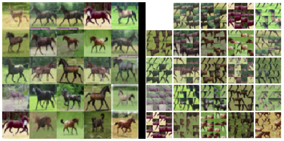
Figure 7: Misclassified example 1. A “deer” image is misclassified as horse.

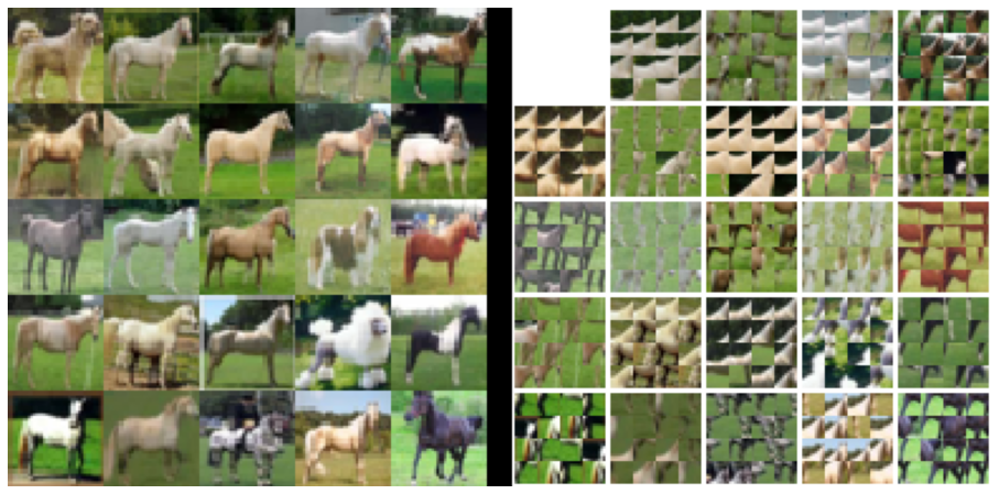
Figure 8: Misclassified example 2. A “dog” image is misclassified as horse.

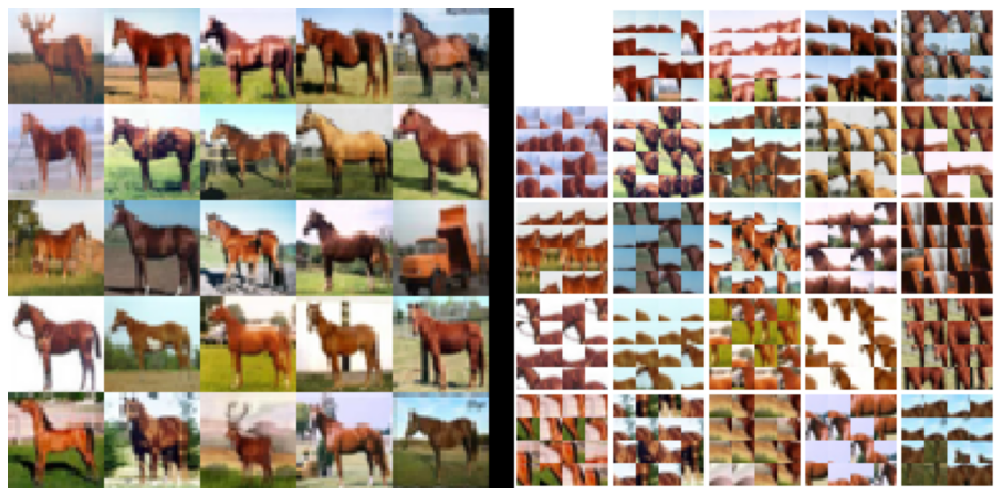
Figure 9: Misclassified example 3. A “deer” image is misclassified as horse.

References

- Andén & Mallat [2014] Joakim Andén and Stéphane Mallat. Deep scattering spectrum. IEEE Transactions on Signal Processing, 62(16):4114–4128, 2014.
- Arora et al. [2019a] Sanjeev Arora, Simon S Du, Wei Hu, Zhiyuan Li, Russ R Salakhutdinov, and Ruosong Wang. On exact computation with an infinitely wide neural net. Advances in Neural Information Processing Systems, 32, 2019a.
- Arora et al. [2019b] Sanjeev Arora, Hrishikesh Khandeparkar, Mikhail Khodak, Orestis Plevrakis, and Nikunj Saunshi. A theoretical analysis of contrastive unsupervised representation learning. arXiv preprint arXiv:1902.09229, 2019b.
- Balestriero & LeCun [2022] Randall Balestriero and Yann LeCun. Contrastive and non-contrastive self-supervised learning recover global and local spectral embedding methods. arXiv preprint arXiv:2205.11508, 2022.
- Bardes et al. [2021] Adrien Bardes, Jean Ponce, and Yann LeCun. Vicreg: Variance-invariance-covariance regularization for self-supervised learning. arXiv preprint arXiv:2105.04906, 2021.
- Belkin & Niyogi [2003] Mikhail Belkin and Partha Niyogi. Laplacian eigenmaps for dimensionality reduction and data representation. Neural computation, 15(6):1373–1396, 2003.
- Bell & Sejnowski [1995] Anthony J Bell and Terrence J Sejnowski. An information-maximization approach to blind separation and blind deconvolution. Neural computation, 7(6):1129–1159, 1995.
- Bengio et al. [2013] Yoshua Bengio, Aaron Courville, and Pascal Vincent. Representation learning: A review and new perspectives. IEEE transactions on pattern analysis and machine intelligence, 35(8):1798–1828, 2013.
- Bordes et al. [2021] Florian Bordes, Randall Balestriero, and Pascal Vincent. High fidelity visualization of what your self-supervised representation knows about. arXiv preprint arXiv:2112.09164, 2021.
- Brendel & Bethge [2019] Wieland Brendel and Matthias Bethge. Approximating cnns with bag-of-local-features models works surprisingly well on imagenet. arXiv preprint arXiv:1904.00760, 2019.
- Cadieu & Olshausen [2012] Charles F Cadieu and Bruno A Olshausen. Learning intermediate-level representations of form and motion from natural movies. Neural computation, 24(4):827–866, 2012.
- Carlsson et al. [2008] Gunnar Carlsson, Tigran Ishkhanov, Vin De Silva, and Afra Zomorodian. On the local behavior of spaces of natural images. International journal of computer vision, 76(1):1–12, 2008.
- Chan et al. [2022] Kwan Ho Ryan Chan, YD Yu, Chong You, Haozhi Qi, John Wright, and Yi Ma. Redunet: A white-box deep network from the principle of maximizing rate reduction. J Mach Learn Res, 23(114):1–103, 2022.
- Chan et al. [2015] Tsung-Han Chan, Kui Jia, Shenghua Gao, Jiwen Lu, Zinan Zeng, and Yi Ma. Pcanet: A simple deep learning baseline for image classification? IEEE transactions on image processing, 24(12):5017–5032, 2015.
- Chefer et al. [2021] Hila Chefer, Shir Gur, and Lior Wolf. Generic attention-model explainability for interpreting bi-modal and encoder-decoder transformers. In Proceedings of the IEEE/CVF International Conference on Computer Vision, pp. 397–406, 2021.
- Chen et al. [2001] Scott Shaobing Chen, David L Donoho, and Michael A Saunders. Atomic decomposition by basis pursuit. SIAM review, 43(1):129–159, 2001.
- Chen & Donoho [1994] Shaobing Chen and David Donoho. Basis pursuit. In Proceedings of 1994 28th Asilomar Conference on Signals, Systems and Computers, volume 1, pp. 41–44. IEEE, 1994.
- Chen et al. [2020a] Ting Chen, Simon Kornblith, Mohammad Norouzi, and Geoffrey Hinton. A simple framework for contrastive learning of visual representations. In International conference on machine learning, pp. 1597–1607. PMLR, 2020a.
- Chen & He [2021] Xinlei Chen and Kaiming He. Exploring simple siamese representation learning. In Proceedings of the IEEE/CVF Conference on Computer Vision and Pattern Recognition, pp. 15750–15758, 2021.
- Chen et al. [2020b] Xinlei Chen, Haoqi Fan, Ross Girshick, and Kaiming He. Improved baselines with momentum contrastive learning. arXiv preprint arXiv:2003.04297, 2020b.
- Chen et al. [2018] Yubei Chen, Dylan M. Paiton, and Bruno A. Olshausen. The sparse manifold transform. In Advances in Neural Information Processing Systems 31: Annual Conference on Neural Information Processing Systems 2018, NeurIPS 2018, December 3-8, 2018, Montréal, Canada, pp. 10534–10545, 2018.
- Chen et al. [2022] Yubei Chen, Adrien Bardes, Zengyi Li, and Yann LeCun. Intra-instance vicreg: Bag of self-supervised image patch embedding. arXiv preprint arXiv:2206.08954, 2022.
- Coates et al. [2011] Adam Coates, Andrew Ng, and Honglak Lee. An analysis of single-layer networks in unsupervised feature learning. In Proceedings of the fourteenth international conference on artificial intelligence and statistics, pp. 215–223. JMLR Workshop and Conference Proceedings, 2011.
- Daubechies [1988] Ingrid Daubechies. Orthonormal bases of compactly supported wavelets. Communications on pure and applied mathematics, 41(7):909–996, 1988.
- de Sa [1994] Virginia R de Sa. Learning classification with unlabeled data. Advances in neural information processing systems, pp. 112–112, 1994.
- De Silva & Carlsson [2004] Vin De Silva and Gunnar E Carlsson. Topological estimation using witness complexes. SPBG, 4:157–166, 2004.
- De Silva & Tenenbaum [2004] Vin De Silva and Joshua B Tenenbaum. Sparse multidimensional scaling using landmark points. Technical report, Technical report, Stanford University, 2004.
- Deerwester et al. [1990] Scott Deerwester, Susan T Dumais, George W Furnas, Thomas K Landauer, and Richard Harshman. Indexing by latent semantic analysis. Journal of the American society for information science, 41(6):391–407, 1990.
- Devlin et al. [2018] Jacob Devlin, Ming-Wei Chang, Kenton Lee, and Kristina Toutanova. Bert: Pre-training of deep bidirectional transformers for language understanding. arXiv preprint arXiv:1810.04805, 2018.
- Dhillon & Modha [2001] Inderjit S. Dhillon and Dharmendra S. Modha. Concept decompositions for large sparse text data using clustering. Machine Learning, 42(1):143–175, 2001.
- DiCarlo & Cox [2007] James J DiCarlo and David D Cox. Untangling invariant object recognition. Trends in cognitive sciences, 11(8):333–341, 2007.
- DiCarlo et al. [2012] James J DiCarlo, Davide Zoccolan, and Nicole C Rust. How does the brain solve visual object recognition? Neuron, 73(3):415–434, 2012.
- Donath & Hoffman [2003] William E Donath and Alan J Hoffman. Lower bounds for the partitioning of graphs. In Selected Papers Of Alan J Hoffman: With Commentary, pp. 437–442. World Scientific, 2003.
- Dumais [2004] Susan T Dumais. Latent semantic analysis. Annual Review of Information Science and Technology (ARIST), 38:189–230, 2004.
- Epshtein & Ullman [2007] Boris Epshtein and Shimon Ullman. Semantic hierarchies for recognizing objects and parts. In 2007 IEEE Conference on Computer Vision and Pattern Recognition, pp. 1–8. IEEE, 2007.
- Ethayarajh [2019] Kawin Ethayarajh. How contextual are contextualized word representations? comparing the geometry of bert, elmo, and gpt-2 embeddings. arXiv preprint arXiv:1909.00512, 2019.
- Fiedler [1973] Miroslav Fiedler. Algebraic connectivity of graphs. Czechoslovak mathematical journal, 23(2):298–305, 1973.
- Freeman et al. [1991] William T Freeman, Edward H Adelson, et al. The design and use of steerable filters. IEEE Transactions on Pattern analysis and machine intelligence, 13(9):891–906, 1991.
- Garrido et al. [2022] Quentin Garrido, Yubei Chen, Adrien Bardes, Laurent Najman, and Yann Lecun. On the duality between contrastive and non-contrastive self-supervised learning. arXiv preprint arXiv:2206.02574, 2022.
- Goroshin et al. [2015a] Ross Goroshin, Joan Bruna, Jonathan Tompson, David Eigen, and Yann LeCun. Unsupervised learning of spatiotemporally coherent metrics. In Proceedings of the IEEE international conference on computer vision, pp. 4086–4093, 2015a.
- Goroshin et al. [2015b] Ross Goroshin, Michael F Mathieu, and Yann LeCun. Learning to linearize under uncertainty. Advances in neural information processing systems, 28, 2015b.
- Gray [1984] Robert M. Gray. Vector quantization. IEEE ASSP Magazine, 1:4–29, 1984.
- Grenander & Miller [2006] Ulf Grenander and Michael I Miller. Pattern theory: from representation to inference. OUP Oxford, 2006.
- Hadsell et al. [2006] Raia Hadsell, Sumit Chopra, and Yann LeCun. Dimensionality reduction by learning an invariant mapping. In 2006 IEEE Computer Society Conference on Computer Vision and Pattern Recognition (CVPR’06), volume 2, pp. 1735–1742. IEEE, 2006.
- HaoChen et al. [2021] Jeff Z HaoChen, Colin Wei, Adrien Gaidon, and Tengyu Ma. Provable guarantees for self-supervised deep learning with spectral contrastive loss. Advances in Neural Information Processing Systems, 34:5000–5011, 2021.
- Hashimoto et al. [2015] Tatsunori B Hashimoto, David Alvarez-Melis, and Tommi S Jaakkola. Word, graph and manifold embedding from markov processes. arXiv preprint arXiv:1509.05808, 2015.
- He et al. [2020] Kaiming He, Haoqi Fan, Yuxin Wu, Saining Xie, and Ross Girshick. Momentum contrast for unsupervised visual representation learning. In Proceedings of the IEEE/CVF conference on computer vision and pattern recognition, pp. 9729–9738, 2020.
- Hénaff et al. [2015] Olivier J. Hénaff, Johannes Ballé, Neil C. Rabinowitz, and Eero P. Simoncelli. The local low-dimensionality of natural images. In 3rd International Conference on Learning Representations, ICLR 2015, San Diego, CA, USA, May 7-9, 2015, Conference Track Proceedings, 2015.
- Hénaff et al. [2019] Olivier J Hénaff, Robbe LT Goris, and Eero P Simoncelli. Perceptual straightening of natural videos. Nature neuroscience, 22(6):984–991, 2019.
- Hénaff et al. [2021] Olivier J Hénaff, Yoon Bai, Julie A Charlton, Ian Nauhaus, Eero P Simoncelli, and Robbe LT Goris. Primary visual cortex straightens natural video trajectories. Nature communications, 12(1):1–12, 2021.
- Hinton [1979] Geoffrey Hinton. Some demonstrations of the effects of structural descriptions in mental imagery. Cognitive Science, 3(3):231–250, 1979.
- Hinton [2021] Geoffrey Hinton. How to represent part-whole hierarchies in a neural network. arXiv preprint arXiv:2102.12627, 2021.
- Hinton [1990] Geoffrey E Hinton. Mapping part-whole hierarchies into connectionist networks. Artificial Intelligence, 46(1-2):47–75, 1990.
- Hinton & Roweis [2002] Geoffrey E Hinton and Sam Roweis. Stochastic neighbor embedding. Advances in neural information processing systems, 15, 2002.
- Huang et al. [2022] Junqiang Huang, Xiangwen Kong, and Xiangyu Zhang. Revisiting the critical factors of augmentation-invariant representation learning. arXiv preprint arXiv:2208.00275, 2022.
- Hyvärinen & Oja [1997] Aapo Hyvärinen and Erkki Oja. A fast fixed-point algorithm for independent component analysis. Neural computation, 9(7):1483–1492, 1997.
- Hyvärinen et al. [2001] Aapo Hyvärinen, Patrik O Hoyer, and Mika Inki. Topographic independent component analysis. Neural computation, 13(7):1527–1558, 2001.
- Hyvärinen et al. [2003] Aapo Hyvärinen, Jarmo Hurri, and Jaakko Väyrynen. Bubbles: a unifying framework for low-level statistical properties of natural image sequences. JOSA A, 20(7):1237–1252, 2003.
- Hyvärinen et al. [2009] Aapo Hyvärinen, Jarmo Hurri, and Patrick O Hoyer. Natural image statistics: A probabilistic approach to early computational vision., volume 39. Springer Science & Business Media, 2009.
- Jegou et al. [2010] Herve Jegou, Matthijs Douze, and Cordelia Schmid. Product quantization for nearest neighbor search. IEEE transactions on pattern analysis and machine intelligence, 33(1):117–128, 2010.
- Jégou et al. [2010] Hervé Jégou, Matthijs Douze, Cordelia Schmid, and Patrick Pérez. Aggregating local descriptors into a compact image representation. In 2010 IEEE computer society conference on computer vision and pattern recognition, pp. 3304–3311. IEEE, 2010.
- Jing et al. [2022] Li Jing, Jiachen Zhu, and Yann LeCun. Masked siamese convnets. arXiv preprint arXiv:2206.07700, 2022.
- Krizhevsky et al. [2017] Alex Krizhevsky, Ilya Sutskever, and Geoffrey E Hinton. Imagenet classification with deep convolutional neural networks. Communications of the ACM, 60(6):84–90, 2017.
- Lazebnik et al. [2006] Svetlana Lazebnik, Cordelia Schmid, and Jean Ponce. Beyond bags of features: Spatial pyramid matching for recognizing natural scene categories. In 2006 IEEE computer society conference on computer vision and pattern recognition (CVPR’06), volume 2, pp. 2169–2178. IEEE, 2006.
- LeCun [2022] Y LeCun. A path towards autonomous machine intelligence. preprint posted on openreview, 2022.
- LeCun et al. [2015] Yann LeCun, Yoshua Bengio, and Geoffrey Hinton. Deep learning. nature, 521(7553):436–444, 2015.
- Lee et al. [2003] Ann B Lee, Kim S Pedersen, and David Mumford. The nonlinear statistics of high-contrast patches in natural images. International Journal of Computer Vision, 54(1):83–103, 2003.
- Levy & Goldberg [2014] Omer Levy and Yoav Goldberg. Linguistic regularities in sparse and explicit word representations. In Proceedings of the eighteenth conference on computational natural language learning, pp. 171–180, 2014.
- Li et al. [2022] Zengyi Li, Yubei Chen, Yann LeCun, and Friedrich T Sommer. Neural manifold clustering and embedding. arXiv preprint arXiv:2201.10000, 2022.
- Li et al. [2019] Zhiyuan Li, Ruosong Wang, Dingli Yu, Simon S Du, Wei Hu, Ruslan Salakhutdinov, and Sanjeev Arora. Enhanced convolutional neural tangent kernels. arXiv preprint arXiv:1911.00809, 2019.
- Ma et al. [2022] Yi Ma, Doris Tsao, and Heung-Yeung Shum. On the principles of parsimony and self-consistency for the emergence of intelligence. Frontiers of Information Technology & Electronic Engineering, 23(9):1298–1323, 2022.
- Mallat [1989] Stephane G Mallat. A theory for multiresolution signal decomposition: the wavelet representation. IEEE transactions on pattern analysis and machine intelligence, 11(7):674–693, 1989.
- Manning [2022] Christopher D. Manning. Human Language Understanding & Reasoning. Daedalus, 151(2):127–138, 05 2022.
- Mante et al. [2008] Valerio Mante, Vincent Bonin, and Matteo Carandini. Functional mechanisms shaping lateral geniculate responses to artificial and natural stimuli. Neuron, 58(4):625–638, 2008.
- Meilă & Shi [2001] Marina Meilă and Jianbo Shi. A random walks view of spectral segmentation. In International Workshop on Artificial Intelligence and Statistics, pp. 203–208. PMLR, 2001.
- Merity et al. [2017] Stephen Merity, Caiming Xiong, James Bradbury, and Richard Socher. Pointer sentinel mixture models. In 5th International Conference on Learning Representations, ICLR 2017, Toulon, France, April 24-26, 2017, Conference Track Proceedings. OpenReview.net, 2017.
- Mikolov et al. [2013a] Tomas Mikolov, Kai Chen, Greg Corrado, and Jeffrey Dean. Efficient estimation of word representations in vector space. arXiv preprint arXiv:1301.3781, 2013a.
- Mikolov et al. [2013b] Tomas Mikolov, Ilya Sutskever, Kai Chen, Greg S Corrado, and Jeff Dean. Distributed representations of words and phrases and their compositionality. Advances in neural information processing systems, 26, 2013b.
- Mumford & Desolneux [2010] David Mumford and Agnès Desolneux. Pattern theory: the stochastic analysis of real-world signals. CRC Press, 2010.
- Ng et al. [2001] Andrew Ng, Michael Jordan, and Yair Weiss. On spectral clustering: Analysis and an algorithm. Advances in neural information processing systems, 14, 2001.
- Olshausen & Field [1996] Bruno A Olshausen and David J Field. Emergence of simple-cell receptive field properties by learning a sparse code for natural images. Nature, 381(6583):607, 1996.
- Olshausen & Field [1997] Bruno A Olshausen and David J Field. Sparse coding with an overcomplete basis set: A strategy employed by v1? Vision research, 37(23):3311–3325, 1997.
- Olshausen & Field [2005] Bruno A Olshausen and David J Field. How close are we to understanding v1? Neural computation, 17(8):1665–1699, 2005.
- Oord et al. [2018] Aaron van den Oord, Yazhe Li, and Oriol Vinyals. Representation learning with contrastive predictive coding. arXiv preprint arXiv:1807.03748, 2018.
- Oyallon & Mallat [2015] Edouard Oyallon and Stéphane Mallat. Deep roto-translation scattering for object classification. In Proceedings of the IEEE Conference on Computer Vision and Pattern Recognition, pp. 2865–2873, 2015.
- Pennington et al. [2014] Jeffrey Pennington, Richard Socher, and Christopher D Manning. Glove: Global vectors for word representation. In Proceedings of the 2014 conference on empirical methods in natural language processing (EMNLP), pp. 1532–1543, 2014.
- Perronnin et al. [2010] Florent Perronnin, Jorge Sánchez, and Thomas Mensink. Improving the fisher kernel for large-scale image classification. In European conference on computer vision, pp. 143–156. Springer, 2010.
- Recht et al. [2019] Benjamin Recht, Rebecca Roelofs, Ludwig Schmidt, and Vaishaal Shankar. Do imagenet classifiers generalize to imagenet? In International Conference on Machine Learning, pp. 5389–5400. PMLR, 2019.
- Roweis & Saul [2000] Sam T Roweis and Lawrence K Saul. Nonlinear dimensionality reduction by locally linear embedding. science, 290(5500):2323–2326, 2000.
- Rumelhart et al. [1986] David E Rumelhart, Geoffrey E Hinton, and Ronald J Williams. Learning representations by back-propagating errors. nature, 323(6088):533–536, 1986.
- Sarzynska-Wawer et al. [2021] Justyna Sarzynska-Wawer, Aleksander Wawer, Aleksandra Pawlak, Julia Szymanowska, Izabela Stefaniak, Michal Jarkiewicz, and Lukasz Okruszek. Detecting formal thought disorder by deep contextualized word representations. Psychiatry Research, 304:114135, 2021.
- Saul & Roweis [2003] Lawrence K Saul and Sam T Roweis. Think globally, fit locally: unsupervised learning of low dimensional manifolds. Journal of machine learning research, 4(Jun):119–155, 2003.
- Schiebinger et al. [2015] Geoffrey Schiebinger, Martin J Wainwright, and Bin Yu. The geometry of kernelized spectral clustering. The Annals of Statistics, 43(2):819–846, 2015.
- Shankar et al. [2020] Vaishaal Shankar, Alex Fang, Wenshuo Guo, Sara Fridovich-Keil, Jonathan Ragan-Kelley, Ludwig Schmidt, and Benjamin Recht. Neural kernels without tangents. In International Conference on Machine Learning, pp. 8614–8623. PMLR, 2020.
- Shi & Malik [2000] Jianbo Shi and Jitendra Malik. Normalized cuts and image segmentation. IEEE Transactions on pattern analysis and machine intelligence, 22(8):888–905, 2000.
- Shuman et al. [2013] David I Shuman, Sunil K Narang, Pascal Frossard, Antonio Ortega, and Pierre Vandergheynst. The emerging field of signal processing on graphs: Extending high-dimensional data analysis to networks and other irregular domains. IEEE signal processing magazine, 30(3):83–98, 2013.
- Shwartz-Ziv et al. [2022] Ravid Shwartz-Ziv, Randall Balestriero, and Yann LeCun. What do we maximize in self-supervised learning? arXiv preprint arXiv:2207.10081, 2022.
- Silva et al. [2006] Jorge Silva, Jorge Marques, and João Lemos. Selecting landmark points for sparse manifold learning. In Advances in neural information processing systems, pp. 1241–1248, 2006.
- Simoncelli & Freeman [1995] Eero P Simoncelli and William T Freeman. The steerable pyramid: A flexible architecture for multi-scale derivative computation. In Proceedings., International Conference on Image Processing, volume 3, pp. 444–447. IEEE, 1995.
- Simoncelli & Olshausen [2001] Eero P Simoncelli and Bruno A Olshausen. Natural image statistics and neural representation. Annual review of neuroscience, 24(1):1193–1216, 2001.
- Simoncelli et al. [1992] Eero P Simoncelli, William T Freeman, Edward H Adelson, and David J Heeger. Shiftable multiscale transforms. IEEE transactions on Information Theory, 38(2):587–607, 1992.
- Smola & Schölkopf [2004] Alex J Smola and Bernhard Schölkopf. A tutorial on support vector regression. Statistics and computing, 14(3):199–222, 2004.
- Sohn & Lee [2012] Kihyuk Sohn and Honglak Lee. Learning invariant representations with local transformations. arXiv preprint arXiv:1206.6418, 2012.
- Stella & Shi [2003] X Yu Stella and Jianbo Shi. Multiclass spectral clustering. In Computer Vision, IEEE International Conference on, volume 2, pp. 313–313. IEEE Computer Society, 2003.
- Tenenbaum et al. [2000] Joshua B Tenenbaum, Vin De Silva, and John C Langford. A global geometric framework for nonlinear dimensionality reduction. science, 290(5500):2319–2323, 2000.
- Thiry et al. [2021] Louis Thiry, Michael Arbel, Eugene Belilovsky, and Edouard Oyallon. The unreasonable effectiveness of patches in deep convolutional kernels methods. arXiv preprint arXiv:2101.07528, 2021.
- Tian et al. [2021] Yuandong Tian, Xinlei Chen, and Surya Ganguli. Understanding self-supervised learning dynamics without contrastive pairs. In International Conference on Machine Learning, pp. 10268–10278. PMLR, 2021.
- Ullman [2007] Shimon Ullman. Object recognition and segmentation by a fragment-based hierarchy. Trends in cognitive sciences, 11(2):58–64, 2007.
- Vladymyrov & Carreira-Perpinán [2013] Max Vladymyrov and Miguel Á Carreira-Perpinán. Locally linear landmarks for large-scale manifold learning. In Joint European Conference on Machine Learning and Knowledge Discovery in Databases, pp. 256–271. Springer, 2013.
- Wainwright et al. [2002] Martin J. Wainwright, Odelia Schwartz, and Eero P. Simoncelli. Natural image statistics and divisive normalization: Modeling nonlinearity and adaptation in cortical neurons. 2002.
- Wang et al. [2010] Jinjun Wang, Jianchao Yang, Kai Yu, Fengjun Lv, Thomas Huang, and Yihong Gong. Locality-constrained linear coding for image classification. In 2010 IEEE computer society conference on computer vision and pattern recognition, pp. 3360–3367. IEEE, 2010.
- Wiskott & Sejnowski [2002] Laurenz Wiskott and Terrence J Sejnowski. Slow feature analysis: Unsupervised learning of invariances. Neural computation, 14(4):715–770, 2002.
- Wu et al. [2018] Zhirong Wu, Yuanjun Xiong, Stella X Yu, and Dahua Lin. Unsupervised feature learning via non-parametric instance discrimination. In Proceedings of the IEEE conference on computer vision and pattern recognition, pp. 3733–3742, 2018.
- Yeh et al. [2021] Chun-Hsiao Yeh, Cheng-Yao Hong, Yen-Chi Hsu, Tyng-Luh Liu, Yubei Chen, and Yann LeCun. Decoupled contrastive learning. arXiv preprint arXiv:2110.06848, 2021.
- Yu et al. [2009] Kai Yu, Tong Zhang, and Yihong Gong. Nonlinear learning using local coordinate coding. Advances in neural information processing systems, 22, 2009.
- Yun et al. [2021] Zeyu Yun, Yubei Chen, Bruno A Olshausen, and Yann LeCun. Transformer visualization via dictionary learning: contextualized embedding as a linear superposition of transformer factors. arXiv preprint arXiv:2103.15949, 2021.
- Zbontar et al. [2021] Jure Zbontar, Li Jing, Ishan Misra, Yann LeCun, and Stéphane Deny. Barlow twins: Self-supervised learning via redundancy reduction. In International Conference on Machine Learning, pp. 12310–12320. PMLR, 2021.
- Zhang et al. [2019] Juexiao Zhang, Yubei Chen, Brian Cheung, and Bruno A Olshausen. Word embedding visualization via dictionary learning. arXiv preprint arXiv:1910.03833, 2019.
- Zou et al. [2012] Will Zou, Shenghuo Zhu, Kai Yu, and Andrew Ng. Deep learning of invariant features via simulated fixations in video. Advances in neural information processing systems, 25, 2012.