On Convergence of Average-Reward Off-Policy Control Algorithms in Weakly Communicating MDPs

Abstract

We show two average-reward off-policy control algorithms, Differential Q-learning (Wan, Naik, & Sutton 2021a) and RVI Q-learning (Abounadi Bertsekas & Borkar 2001), converge in weakly communicating MDPs. Weakly communicating MDPs are the most general MDPs that can be solved by a learning algorithm with a single stream of experience. The original convergence proofs of the two algorithms require that the solution set of the average-reward optimality equation only has one degree of freedom, which is not necessarily true for weakly communicating MDPs. To the best of our knowledge, our results are the first showing average-reward off-policy control algorithms converge in weakly communicating MDPs. As a direct extension, we show that average-reward options algorithms for temporal abstraction introduced by Wan, Naik, & Sutton (2021b) converge if the Semi-MDP induced by options is weakly communicating.

1 Introduction

Modern reinforcement learning algorithms are designed to maximize the agent’s goal in either the episodic setting or the continuing setting. In both settings, there is an agent continually interacting with its world, which is usually assumed to be a Markov Decision Process (MDP). For episodic problems, there is a special terminal state and a set of start states. If the agent reaches the terminal state, it will be reset to one of the start states. Continuing problems are different in that there is no terminal state, and the agent will never be reset by the world. For continuing problems, two commonly considered objectives are the discounted objective and the average-reward objective. The discount factor in the discounted objective has been observed to be deprecated in the function approximation control setting, suggesting that the average-reward objective might be more suitable for continuing problems.

In this paper, we extend the convergence results of two off-policy control algorithms for the average-reward objective from a sub-class of MDPs to the most general class of MDPs that could be solved by algorithms learning from a single stream of experience. These algorithms learn a policy that achieves the best possible average-reward rate, using data generated by some other policy that the agent may not have control of. Designing convergent off-policy algorithms for the average-reward objective is challenging. While there are several off-policy learning algorithms in the literature, the only known convergent algorithms are SSP Q-learning and RVI Q-learning, both by Abounadi, Bertsekas, & Borkar (2001), the algorithm by Ren & Krogh (2001), and Differential Q-learning by Wan, Naik, & Sutton (2021a). Others either do not have a convergence theory (Schwartz 1993, Singh 1994; Bertsekas & Tsitsiklis 1996, Das 1999) or have incorrect proof (Yang 2016, Gosavi 2004).

The algorithm by Ren & Krogh (2001) requires knowledge of properties of the MDP which are not typically known. The convergence of SSP Q-learning requires knowing a state that is recurrent under all policies. The convergence of the RVI Q-learning algorithm (Abounadi et al. 2001) was developed for unichain MDPs, which just means that the Markov chain induced by any stationary policy is unichain . The convergence of Differential Q-learning (Wan et al. 2021a) requires a weaker assumption – the solution set of the average-reward optimality equation (formally defined later in equation 2) only has one degree of freedom (all the solutions are different by a constant vector). This assumption can be satisfied if, for example, all optimal policies are unichain. It is clear that RVI Q-learning also converges under this assumption.

It is not rare that the solution set of the average-reward optimality equation has more than one degree of freedom (e.g., the MDP at the bottom of Figure 1). In this case, the proofs of RVI Q-learning and Differential Q-learning would not go through. Technically, this is because both two proofs require that the uniqueness of the solution of the action values up to an additive constant (one degree of freedom) in the average-reward optimality equation, so that there is a unique equalibrium in the ordinary differential equations associated with the two algorithms.

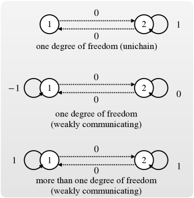
Figure 1: Examples of three different types of MDPs. In each of the three MDPs, there are two states marked by two circles respectively. There are two actions solid and dashed, both causing deterministic effects. Top: The solution set of $q$ in the average-reward optimality equation (equation 2) is $\{q(1,\texttt{dashed})=c-1,q(2,\texttt{solid})=c,q(2,\texttt{{dashed}})=c-2,\forall c\in\mathbb{R}\}$ and has one degree of freedom. The Markov chain under every stationary policy is unichain. Middle: The solution set of $q$ is $\{q(1,\texttt{solid})=c-3,q(1,\texttt{dashed})=c-1,q(2,\texttt{solid})=c,q(2,\texttt{{dashed}})=c-2,\forall c\in\mathbb{R}\}$ and has one degree of freedom. The MDP is weakly-communicating. Down: The solution set of $q$ is has more than one degree of freedom. Note that both $\{q(1,\texttt{solid})=0,q(1,\texttt{dashed})=-2,q(2,\texttt{solid})=-1,q(2,\texttt{dashed})=-1\}$ and $\{q(1,\texttt{solid})=0,q(1,\texttt{dashed})=-1,q(2,\texttt{solid})=0,q(2,\texttt{dashed})=-1\}$ are solutions of $q$ in equation 2 and these two solutions are not different by a constant vector. The MDP is weakly-communicating.

A more general class of MDPs, called weakly communicating MDPs, may have more than a single degree of freedom in the solution set of the associated optimality equation. The definition of these MDPs is also natural: except for a possibly empty set of states that are transient under every policy, all states are reachable from every other state in a finite number of steps with a non-zero probability. It has been observed that the set of weakly communicating MDPs is the most general set of MDPs such that there exists a learning algorithm that can, using a single stream of experience, guarantee to identify a policy that achieves the optimal average reward rate in the MDP (Barlett & Tewari 2009).

In this paper, we show the convergence of RVI Q-learning and Differential Q-learning in weakly communicating MDPs, without requiring any additional assumptions compared with their original convergence theories. Two key steps in our proof are 1) showing that the solution sets of the two algorithms are non-empty, closed, bounded, and connected, and 2) showing that $0$ is the unique solution for the average-reward optimality equation when all rewards are $0$. With these two results, we use asynchronous stochastic approximation results by Borkar (2009) to show convergence to the solution sets. As a direct extension of the above results, we also show the convergence of two algorithms that extend the Differential Q-learning algorithm to the options framework, introduced by Wan et al. (2021b), if the Semi-MDP induced by a given MDP and a given set of options is weakly communicating.

2 Preliminaries

Consider a finite Markov decision process, defined by the tuple $\mathcal{M}\doteq(\mathcal{S},\mathcal{A},\mathcal{R},p)$, where $\mathcal{S}$ is a set of states, $\mathcal{A}$ is a set of actions, $\mathcal{R}$ is a set of rewards, and $p:\mathcal{S}\times\mathcal{R}\times\mathcal{S}\times\mathcal{A}\to[0,1]$ is the dynamics of the MDP. At each time step $t$, the agent observes the state of the MDP $S_{t}\in\mathcal{S}$ and chooses an action $A_{t}\in\mathcal{A}$ using some policy $b:\mathcal{A}\times\mathcal{S}\rightarrow[0,1]$, then receives from the environment a reward $R_{t+1}\in\mathcal{R}$ and the next state $S_{t+1}\in\mathcal{S}$, and so on. The transition dynamics are defined as $p(s^{\prime},r\mid s,a)\doteq\Pr(S_{t+1}=s^{\prime},R_{t+1}=r\mid S_{t}=s,A_{t}=a)$ for all $s,s^{\prime}\in\mathcal{S},a\in\mathcal{A}$, and $r\in\mathcal{R}$. Denote the set of stationary Markov policies $\Pi$.

The reward rate of a policy $\pi$ starting from a given start state $s$ can be defined as:

$$r(\pi,s)\doteq\lim_{n\to\infty}\frac{1}{n}\sum_{t=1}^{n}\mathbb{E}[R_{t}\mid S_{0}=s,A_{0:t-1}\sim\pi].$$ (1)

Given an arbitrary MDP, the agent may not even be able to visit all states and would therefore miss the chance of learning, for every state $s$, a policy that achieves the optimal reward rate $\sup_{\pi}r(\pi,s)$ and the agent can at most learn an optimal policy for a set of states, each of which is reachable from every other state. Such a set of states is often called communicating. Formally speaking, we say a set of states communicating, if there exists a policy such that moving from either one state in the set to the other one in the set in a finite number of steps has a positive probability. If the entire state space of an MDP is communicating, we say the MDP communicating. Weakly communicating MDPs generalize over communicating MDPs. In weakly communicating MDPs, in addition to a closed communicating set of states, there is a possibly empty set of states that are transient under every policy.

For weakly communicating MDPs, there exists a unique optimal reward rate $r_{*}$, which does not depend on the start state. We say a policy is optimal if it achieves $r_{*}$ regardless of the start state. The goal of an off-policy control algorithm is to learn an optimal policy from the stream of experience $\ldots,S_{t},A_{t},R_{t+1},S_{t+1},\ldots$ generated by a behavior policy that is not necessarily the same as the agent’s learned policy. Both RVI Q-learning and Differential Q-learning achieve this goal by solving $\bar{r}$ and $q$ in the optimality equation:

$$q(s,a) =\sum_{s^{\prime},r}p(s^{\prime},r\mid s,a)(r-\bar{r}+\max_{a^{\prime}}q(s^{\prime},a^{\prime})),\quad\forall\ s\in\mathcal{S},a\in\mathcal{A}.$$ (2)

It is known that $r_{*}$ is the unique solution of $\bar{r}$ and any greedy policy w.r.t. any solution of $q$ is an optimal policy. In addition, shifting any solution of $q$ by any constant vector results in the other solution of $q$. Finally, unlike in unichain MDPs, where all solutions of $q$ are different by some constant vector, in weakly communicating MDPs, solutions of $q$ may have multiple degrees of freedom. That is, if $q_{1},q_{2}$ are both solutions of $q$, it is possible that $q_{1}\neq q_{2}+ce,\forall\ c\in\mathbb{R}$, where $e$ denotes the all-one vector.

If the agent has a set of options, it may choose to execute these options. Each option $o$ in $\mathcal{O}$ has two components: the option’s policy $\pi^{o}:\mathcal{A}\times\mathcal{S}\to[0,1]$, and the termination probability $\beta^{o}:\mathcal{S}\to[0,1]$. For simplicity, for any $s\in\mathcal{S},o\in\mathcal{O}$, we use $\pi(a\mid s,o)$ to denote $\pi^{o}(a,s)$ and $\beta(s,o)$ to denote $\beta^{o}(s)$. If the agent executes option $o$ at state $s$, the option’s policy is followed, until the option terminates. Let $\mathcal{L}$ be the set of all possible lengths of options and $\mathcal{\hat{R}}$ be the set of all possible cumulative rewards. Note that $\mathcal{L}$ and $\mathcal{\hat{R}}$ are possibly countably infinite. Let $\hat{p}(s^{\prime},r,l\mid s,o)$ be, when executing option $o$ starting from state $s$, the probability of terminating at state $s^{\prime}$, with cumulative reward $r$ and length $l$. Formally, for any $s,s^{\prime}\in\mathcal{S},o\in\mathcal{O},r\in\mathcal{\hat{R}},l\in\mathcal{L}$, $\hat{p}$ can be defined recursively in the following way:

$$\hat{p}(s^{\prime},r,l\mid s,o)\doteq\sum_{a}\pi(a\mid s,o)\sum_{\tilde{s},\tilde{r}}p(\tilde{s},\tilde{r}\mid s,a)$$

$$[\beta(\tilde{s},o)\mathbf{I}(\tilde{s}=s^{\prime},\tilde{r}=r,\tilde{l}=1)+(1-\beta(\tilde{s},o))\hat{p}(s^{\prime},r-\tilde{r},l-1\mid\tilde{s},o)],$$ (3)

where $\mathbf{I}$ is an indicator function.

An MDP $\mathcal{M}$ and a set of options $\mathcal{O}$ results in a Semi-MDP (SMDP) $\hat{\mathcal{M}}\doteq(\mathcal{S},\mathcal{O},\mathcal{L},\mathcal{\hat{R}},\hat{p})$.

Given an MDP and a set of options, if the agent chooses options using a meta policy, which is a policy that chooses from options, ${\pi}:\mathcal{O}\times\mathcal{S}\to[0,1]$ and executes these options, we denote the sequence of option transitions by $\ldots,\hat{S}_{n},\hat{O}_{n},\hat{R}_{n+1},\hat{S}_{n+1},\ldots$. For the associated SMDP, the reward rate of $\pi$ given a start state $s$ can be defined as $r^{C}(\pi,s)\doteq\lim_{t\to\infty}\mathbb{E}_{\pi}[\sum_{i=1}^{t}R_{i}\mid S_{0}=s]/t$ or $r(\pi,s)\doteq\lim_{n\to\infty}\mathbb{E}_{\pi}[\sum_{i=0}^{n}\hat{R}_{i}\mid\hat{S}_{0}=s]/\mathbb{E}_{\pi}[\sum_{i=0}^{n}\hat{L}_{i}\mid\hat{S}_{0}=s]$. Both limits exist and are equivalent (by Puterman’s (1994) Propositions 11.4.1 and 11.4.7) under the following assumption:

Assumption 1.

For each option $o\in\mathcal{O}$, when executing the option, there is a non-zero probability of terminating the option after at most ${\left\lvert\mathcal{S}\right\rvert}$ stages, regardless of the state at which this option is initiated.

Proposition 1.

Under 1, the expected value as well as the variance of the execution time and cumulative reward of every option at each state exist and are finite.

We say an SMDP is weakly communicating if the MDP with state space $\mathcal{S}$, action space $\mathcal{O}$, reward space $\mathcal{\hat{R}}$, and transition function $\sum_{l}\hat{p}(s,r,l\mid s,o)$ is weakly communicating. Just as in the MDP setting, if the SMDP is weakly communicating, the optimal reward rate $\hat{r}_{*}\doteq\sup_{\pi\in\hat{\Pi}}r(\pi,s)$, where $\hat{\Pi}$ denotes the set of stationary Markov meta policies, does not depend on the start state $s$. In addition, the solutions of $q$ may not be different by a constant vector. Given an MDP and a set of options, the goal of the off-policy control problem is to find a policy that achieves $\hat{r}_{*}$. Inter-option Differential Q-learning achieves this goal by solving the optimality equation for SMDPs (Puterman 1994):

$$q(s,o) =\sum_{s^{\prime},r,\,l}\hat{p}(s^{\prime},r,\,l\mid s,o)\big{(}r-\bar{r}\cdot l+\max_{o^{\prime}}q(s^{\prime},o^{\prime})\big{)},$$ (4)

where $q$ and $\bar{r}$ denote estimates of the option-value function and the reward rate respectively. Just as in the MDP setting, $\bar{r}$ has $\hat{r}_{*}$ as its unique solution, and solutions of $q$ may not be different by a constant vector.

Intra-option Differential-learning finds an optimal policy by solving the intra-option optimality equation.

$$q(s,o) =\sum_{a}\pi(a\mid s,o)\sum_{s^{\prime},r}p(s^{\prime},r\mid s,a)(r-\bar{r}+u^{q}_{*}(s^{\prime},o)),\quad\forall\ s\in\mathcal{S},o\in\mathcal{O},$$ (5)

where

$$u^{q}_{*}(s^{\prime},o) \doteq\big{(}1-\beta(s^{\prime},o)\big{)}q(s^{\prime},o)+\beta(s^{\prime},o)\max_{o^{\prime}}q(s^{\prime},o^{\prime}).$$ (6)

The following proposition shows that the set of solutions of equation 5 is the same as that of equation 4.

Proposition 2.

Any solution of equation 4 is also a solution of equation 5 and vice versa.

3 Convergence Results

In this section, we present convergence theories of Differential Q-learning and RVI Q-learning in weakly communicating MDPs, and theories of the two option extensions of Differential Q-learning in weakly communicating SMDPs. Empirical results verifying the convergence of the two MDP algorithms are presented in Appendix B.

Differential Q-learning updates a table of estimates $Q_{t}:\mathcal{S}\times\mathcal{A}\to\mathbb{R}$ as follows:

$$Q_{t+1}(S_{t},A_{t}) \doteq Q_{t}(S_{t},A_{t})+\alpha_{\nu(t,S_{t},A_{t})}\delta_{t},$$ (7)

$$Q_{t+1}(s,a) \doteq Q_{t}(s,a),\ \forall\ s,a\neq S_{t},A_{t},$$

where $\nu(t,S_{t},A_{t})$ is the number of times $S_{t},A_{t}$ has been visited before time step $t$, $\{\alpha_{\nu(t,S_{t},A_{t})}\}$ is a step-size sequence, and $\delta_{t}$, the temporal-difference (TD) error, is:

$$\delta_{t}\doteq R_{t+1}-\bar{R}_{t}+\max_{a}Q_{t}(S_{t+1},a)-Q_{t}(S_{t},A_{t}),$$ (8)

where $\bar{R}_{t}$ is a scalar estimate of $r_{*}$, updated by:

$$\bar{R}_{t+1}\doteq\bar{R}_{t}+\eta\alpha_{\nu(t,S_{t},A_{t})}\delta_{t},$$ (9)

and $\eta$ is a positive constant.

We now present the convergence theory of Differential Q-learning. We first state the required assumptions, which are also required by the original convergence theory of Differential Q-learning by Wan et al. (2021a).

Assumption 2.

For all $n\geq 0$, $\alpha_{n}>0$, $\sum_{n=0}^{\infty}\alpha_{n}=\infty$, and $\sum_{n=0}^{\infty}\alpha_{n}^{2}<\infty$.

Assumption 3.

Let $[\cdot]$ denote the integer part of $(\cdot)$, for $x\in(0,1)$, $\sup_{n}\frac{\alpha_{[xn]}}{\alpha_{n}}<\infty$ and $\frac{\sum_{n=0}^{[ym]}\alpha_{n}}{\sum_{n=0}^{m}\alpha_{n}}\to 1$ uniformly in $y\in[x,1]$.

Assumption 4.

There exists $\Delta>0$ such that

$$\liminf_{n\to\infty}\frac{\nu(n,s,a)}{n+1}\geq\Delta,$$

a.s., for all $s\in\mathcal{S},a\in\mathcal{A}$. Furthermore, for all $x>0$, let $N(n,x)=\min\left\{m>n:\sum_{k=n+1}^{m}\alpha_{k}\geq x\right\},$ the limit $\lim_{n\to\infty}\left(\sum_{k=\nu(n,s,a)}^{\nu(N(n,x),s,a)}\alpha_{k}\right)/\left(\sum_{k=\nu(n,s^{\prime},a^{\prime})}^{\nu(N(n,x),s^{\prime},a^{\prime})}\alpha_{k}\right)$ exists a.s. for all $s,s^{\prime}\in\mathcal{S},a,a^{\prime}\in\mathcal{A}$.

Theorem 1.

If $\mathcal{M}$ is communicating and Assumptions 2–4 hold, the Differential Q-learning algorithm (Equations 7–9) converges, almost surely, $\bar{R}_{t}$ to $r_{*}$, $Q_{t}$ to the set of solutions of equation 2 and

$$r_{*}-\bar{R}_{0} =\eta\left(\sum_{s,a}q(s,a)-\sum_{s,a}Q_{0}(s,a)\right),$$ (10)

and $r(\pi_{t},s)$ to $r_{*}$, for all $s\in\mathcal{S}$, where $\pi_{t}$ is any greedy policy w.r.t. $Q_{t}$.

Remark: If the MDP is weakly communicating, that is, it contains transient states, the agent eventually reaches the closed communicating state and never returns to the transient states. Elements in $Q_{n}$ that are associated with the closed communicating set converge to a set that depends on the values of $Q$ and $\bar{R}$ when the MDP reaches the closed communicating set for the first time. Other elements in $Q_{n}$ would only be visited for a finite number of times and can not be guaranteed to converge to their correct values by any learning algorithm. Other conclusions of the theorem remain unchanged. This observation on weakly communicating MDPs also applies to Theorems 2–4.

The update rules of RVI Q-learning are

$$Q_{t+1}(S_{t},A_{t}) \doteq Q_{t}(S_{t},A_{t})+\alpha_{\nu(t,S_{t},A_{t})}\delta_{t}(S_{t},A_{t}),$$ (11)

$$Q_{t+1}(s,a) \doteq Q_{t}(s,a),\ \forall\ s,a\neq S_{t},A_{t},$$

where

$$\delta_{t}(S_{t},A_{t})\doteq R_{t+1}-f(Q_{t})+\max_{a}Q_{t}(S_{t+1},a)-Q_{t}(S_{t},A_{t}),$$ (12)

and $f:\mathcal{S}\times\mathcal{A}\to\mathbb{R}$ satisfies the following assumption.

Assumption 5.

1) $f$ is $L$-Lipschitz, 2) there exists a positive scalar $u$ s.t. $f(e)=u$ and $f(x+ce)=f(x)+cu$, and 3) $f(cx)=cf(x),\forall c\in\mathbb{R}$.

Theorem 2.

If $\mathcal{M}$ is communicating and Assumptions 2–5 hold, then the RVI Q-learning algorithm (Equations 11–12) converges, almost surely, $\bar{R}_{t}$ to $r_{*}$, $Q_{t}$ to the set of solutions of equation 2 and

$$r_{*} =f(q),$$ (13)

and $r(\pi_{t},s)$ to $r_{*}$, for all $s\in\mathcal{S}$, where $\pi_{t}$ is any greedy policy w.r.t. $Q_{t}$.

Now consider option extensions of Differential Q-learning. Given an SMDP $\hat{\mathcal{M}}=(\mathcal{S},\mathcal{O},\mathcal{L},\mathcal{\hat{R}},\hat{p})$, inter-option Differential Q-learning maintains estimates of option values, and, inspired by Schweitzer (1971), updates estimates using scaled TD errors:

$$Q_{n+1}(\hat{S}_{n},\hat{O}_{n}) \doteq Q_{n}(\hat{S}_{n},\hat{O}_{n})+\alpha_{\nu(n,\hat{S}_{n},\hat{O}_{n})}\delta_{n}/L_{n}(\hat{S}_{n},\hat{O}_{n}),$$ (14)

$$Q_{n+1}(s,o) \doteq Q_{n}(s,o),\ \forall\ s,o\neq\hat{S}_{n},\hat{O}_{n},$$

$$\bar{R}_{n+1} \doteq\bar{R}_{n}+\eta\alpha_{\nu(n,\hat{S}_{n},\hat{O}_{n})}\delta_{n}/L_{n}(\hat{S}_{n},\hat{O}_{n}),$$ (15)

where $\nu(n,\hat{S}_{n},\hat{O}_{n})$ is the number of visits to state-option pair $(\hat{S}_{n},\hat{O}_{n})$ before stage $n$, $L_{n}(\cdot,\cdot)$ comes from an additional vector of estimates $L:\mathcal{S}\times\mathcal{O}\to\mathbb{R}$ that approximate the expected lengths of state-option pairs, updated by:

$$L_{n+1}(\hat{S}_{n},\hat{O}_{n})\doteq L_{n}(\hat{S}_{n},\hat{O}_{n})+\beta_{\nu(n,\hat{S}_{n},\hat{O}_{n})}(\hat{L}_{n}-L_{n}(\hat{S}_{n},\hat{O}_{n})),$$ (16)

where $\{\beta_{n}\}$ is the other step-size sequence. The TD-error $\delta_{n}$ in equation 14 and equation 15 is

$$\delta_{n} \doteq\hat{R}_{n}-L_{n}(\hat{S}_{n},\hat{O}_{n})\bar{R}_{n}+\max_{o}Q_{n}(\hat{S}_{n+1},o)-Q_{n}(\hat{S}_{n},\hat{O}_{n}),$$ (17)

Theorem 3.

If $\hat{\mathcal{M}}$ is communicating, Assumptions 1–4 hold, except for using $\nu(n,s,o)$ instead of $\nu(t,s,a)$, and that $0\leq\beta_{n}\leq 1$, $\sum_{n}\beta_{n}=\infty$, and $\sum_{n}\beta_{n}^{2}<\infty$, inter-option Differential Q-learning (Equations 14-17) converges, almost surely, $Q_{n}$ to the set of solutions of equation 4 and

$$\hat{r}_{*}-\bar{R}_{0} =\eta\left(\sum_{s,o}q(s,o)-\sum_{s,o}Q_{0}(s,o)\right),$$ (18)

$\bar{R}_{n}$ to $\hat{r}_{*}$, and $r(\pi_{n},s)$ to $\hat{r}_{*}$ where $\pi_{n}$ is a greedy policy w.r.t. $Q_{n}$.

Intra-option Differential Q-learning also maintains estimates of option values. However, instead of updating the estimates using option transitions, it updates for all options using each action transition $(S_{t},O_{t},A_{t},R_{t+1},S_{t+1})$.

$$Q_{t+1}(S_{t},o) \doteq Q_{t}(S_{t},o)+\alpha_{\nu(t,S_{t},o)}\rho_{t}(o)\delta_{t}(o),\quad\forall\ o\in\mathcal{O},$$ (19)

$$Q_{t+1}(s,o) \doteq Q_{t}(s,o),\quad\forall\ s\in\mathcal{S},o\in\mathcal{O},$$

$$\bar{R}_{t+1} \doteq\bar{R}_{t}+\eta\sum_{o\in\mathcal{O}}\alpha_{\nu(t,S_{t},o)}\rho_{t}(o)\delta_{t}(o),$$ (20)

where $\{\alpha_{t}\}$ is a step-size sequence, $\rho_{t}(o)\doteq\frac{\pi(A_{t}|S_{t},o)}{\pi(A_{t}|S_{t},O_{t})}$ is the importance sampling ratio, and:

$$\delta_{t}(o)\doteq R_{t+1}-\bar{R}_{t}+u^{Q_{t}}_{*}(S_{t+1},o)-Q_{t}(S_{t},o),$$ (21)

where $u_{*}^{Q_{t}}$ is defined in equation 6.

Theorem 4.

If $\hat{\mathcal{M}}$ is communicating, Assumptions 1–4 hold, except for using $\nu(t,s,o)$ instead of $\nu(t,s,a)$, intra-option Differential Q-learning (Equations 19-21) converges, almost surely, $Q_{t}$ to the set of solutions of equation 4 and equation 18, $\bar{R}_{t}$ to $\hat{r}_{*}$, and $r(\pi_{t},s)$ to $\hat{r}_{*}$ where $\pi_{t}$ is a greedy policy w.r.t. $Q_{t}$.

4 Characterization of the Solution Set

In this section, we characterize the sets that the algorithms described in the previous section converge to. This section plays a key role in showing their convergence.

We consider the set of solutions of $q$ in the SMDP optimality equation (equation 4) and

$$\hat{r}_{*} =f(q),$$ (22)

where $f:\mathcal{S}\times\mathcal{O}\to\mathbb{R}$ satisfies 5. It is clear that equation 4 generalizes over equation 2 and equation 22 generalizes over equation 10, equation 13, and equation 18. And thus the characterization of $\mathcal{Q}_{\infty}$ applies to the sets that action/option values in the aforementioned algorithms are claimed to converge to in Theorems 1–4.

It is known that if the SMDP is weakly communicating, equation 4 has $\hat{r}_{*}$ as its unique solution of $\bar{r}$. For $q$, it has been shown by Schweitzer & Federgruen (1978) (we will refer to this work multiple times and thus we use a shorthand “S&F” for simplicity from now on) in their Theorem 4.2 that the set of solutions of $q$ in equation 4 is closed, unbounded, connected, and possibly non-convex. The next theorem characterizes $\mathcal{Q}_{\infty}$.

Theorem 5.

If the SMDP is weakly communicating and 5 holds, $\mathcal{Q}_{\infty}$ is non-empty, closed, bounded, connected, and possibly non-convex.

Before presenting the proof, first note that our convergence proof does not rely on the convexity property and we defer the proof of non-convexity to Section A.5.

Proof.

First, $\mathcal{Q}_{\infty}$ is non-empty. To see this point, note that for any solution of $q$ in equation 4, $q_{*}$, $q_{*}+ce$ is also a solution for any $c\in\mathbb{R}$ and thus there must be a $c$ such that equation 22 holds because $f(x+ce)=f(x)+cu$ for any $x,c$.

$\mathcal{Q}_{\infty}$ is closed because the set of solutions of $q$ in equation 4 is closed by S&F, the set of solutions of $q$ in equation 22 is closed because $f$ is Lipschitz and is thus continuous, and the intersection of two closed sets is closed.

Boundedness

We now show that $\mathcal{Q}_{\infty}$ is bounded. For any $q\in\mathcal{Q}_{\infty}$, let $v(s)\doteq\max_{o}q(s,o)$. Rewrite the option-value optimality equation (Equation 4) using $v$ instead of $q$, we have,

$$v(s) =\max_{o}\sum_{s^{\prime},r,l}\hat{p}(s^{\prime},r,l\mid s,o)(r-l\hat{r}_{*}+v(s^{\prime})),\forall\ s\in\mathcal{S}.$$ (23)

The above equation is known as the state-value optimality equation.

It is easy to verify that

$$q(s,o)=\sum_{s^{\prime},r,l}\hat{p}(s^{\prime},r,l\mid s,o)(r-l\hat{r}_{*}+v(s^{\prime})).$$ (24)

Using this fact, rewrite Equation 22 using $v$ instead of $q$, we have,

$$\hat{r}_{*} =f(\tilde{r}+\tilde{P}v),$$ (25)

where

$$\tilde{r}(s,o) \doteq\sum_{s^{\prime},r,l}\hat{p}(s^{\prime},r,l\mid s,o)(r-l\hat{r}_{*}),$$

$$\tilde{P}(s,o,s^{\prime}) \doteq\sum_{r,l}\hat{p}(s^{\prime},r,l\mid s,o).$$

Denote the set of solutions of $v$ in equation 23 by $\mathcal{V}$. Denote the set of solutions of $v$ in Equation 23 and Equation 25 by $\mathcal{V}_{\infty}$. If $\mathcal{V}_{\infty}$ is bounded, $\mathcal{Q}_{\infty}$ is also bounded because any $q\in\mathcal{Q}_{\infty}$ can be obtained from a solution of $v\in\mathcal{V}_{\infty}$ with a linear operation in view of Equation 24.

In order to show boundedness, We will need the following two lemmas to proceed. These two lemmas are similar to Theorem 4.1 (c) and Theorem 5.1 in S&F, except that 1) the ’$\max$’ operates over the set of all optimal policies, instead of the set of all deterministic optimal policies as in Theorem 4.1 (c), and 2) we consider the set of weakly communicating SMDPs while S&F considers general multi-chain SMDPs. The proofs are also essentially the same. For completeness, we provide the proofs for these two lemmas in Sections A.3, A.4.

To formally state the Lemma 1, we will first introduce some definitions.

For any $\pi\in\hat{\Pi}$, let $P_{\pi}$ denote the ${\left\lvert\mathcal{S}\right\rvert}\times{\left\lvert\mathcal{S}\right\rvert}$ transition probability matrix under policy $\pi$. That is,

$$P_{\pi}(s,s^{\prime})\doteq\sum_{o,r,l}\pi(o\mid s)\hat{p}(s^{\prime},r,l\mid s,o).$$ (26)

Let $P_{\pi}^{\infty}$ be the limiting matrix of $P_{\pi}$, which is the Cesaro limit of the sequence $\{P_{\pi}^{i}\}_{i=1}^{\infty}$:

$$P_{\pi}^{\infty}\doteq\lim_{n\to\infty}\frac{1}{n}\sum_{i=0}^{n-1}P_{\pi}^{i}.$$ (27)

Because $\mathcal{S}$ is finite, the Cesaro limit exists and $P_{\pi}^{\infty}$ is a stochastic matrix (has row sums equal to 1).

Let $l_{\pi}(s)\doteq\sum_{o,s^{\prime},r,l}\pi(o\mid s)\hat{p}(s^{\prime},r,l\mid s,o)l$. And let the fundamental matrix $Z_{\pi}\doteq(I-P_{\pi}^{\infty}+P_{\pi}^{\infty})^{-1}=I+\lim_{\gamma\uparrow 1}\sum_{n=1}^{\infty}\gamma^{n}(P_{\pi}^{n}-P_{\pi}^{\infty})$.

Lemma 1.

If the SMDP is weakly communicating, $v$ is a solution of equation 23 if and only if

$$v(s)=\max_{\pi\in\hat{\Pi}_{*}}[Z_{\pi}(r_{\pi}-l_{\pi}\hat{r}_{*})+P_{\pi}^{\infty}v](s),\forall\ s\in\mathcal{S}.$$ (28)

In order to state Lemma 2 formally, we need the following definitions. Define the Bellman error for a state $s\in\mathcal{S}$ given a policy $\pi\in\hat{\Pi}$ and some $v\in\mathbb{R}^{{\left\lvert\mathcal{S}\right\rvert}}$, $b_{v,\pi}(s)$, as follows:

$$b_{v,\pi}(s) \doteq[r_{\pi}-l_{\pi}\hat{r}_{*}+P_{\pi}^{\infty}v-v](s).$$

Define $R_{\pi}$ as the set of recurrent states for $P_{\pi}^{\infty}$. That is,

$$R_{\pi} \doteq\{s\mid P_{\pi}^{\infty}(s,s)>0\}.$$

Let $\hat{\Pi}_{*}$ denote the set of optimal meta policies. Define ${R}_{*}$ as the set of states that are recurrent under some optimal meta policy:

$${R}_{*} \doteq\{s\mid s\in R_{\pi}\text{ for some policy }\pi\in\hat{\Pi}_{*}\}.$$

By Theorem 3.2 (b) in S&F, there exists a policy $\pi\in\hat{\Pi}_{*}$ such that $R_{\pi}={R}_{*}$. For any $\pi\in\hat{\Pi}$, let $n(\pi)$ be the number of recurrent classes for $P_{\pi}^{\infty}$. Further, define the least number of recurrent classes induced by any optimal meta policy that induces the set of recurrent states ${R}_{*}$:

$$n_{*}\doteq\min\{n(\pi)\mid\pi\in\hat{\Pi}_{*},R_{\pi}={R}_{*}\}.$$

Denote $\hat{\Pi}_{**}$ as the set of policies that have ${R}_{*}$ as their sets of recurrent states and that have $n_{*}$ recurrent classes. That is,

$$\hat{\Pi}_{**}\doteq\{\pi\in\hat{\Pi}_{*}\mid R_{\pi}={R}_{*},n(\pi)=n_{*}\}.$$

Theorem 3.2 (d) by S&F shows that all policies within $\hat{\Pi}_{**}$ share the same collection of recurrent classes. Denote the collection of recurrent classes as $\{R_{*\alpha}\mid 1,2,\cdots,n_{*}\}$. The following lemma shows that the solution set of equation 23 has $n_{*}$ degrees of freedom.

Lemma 2.

If the SMDP is weakly communicating, suppose $v$ and $v+x$ are both solutions of equation 23, then there exists $n_{*}$ constants $y_{1},y_{2},\cdots,y_{n_{*}}$ such that

$$x(s) =y_{\alpha},i\in R_{*\alpha},\quad\alpha=1,\dots,n_{*}$$ (29)

$$x(s) =\max_{\pi\in\hat{\Pi}_{*}}[Z_{\pi}b_{v,\pi}](s)+\sum_{\beta=1}^{n_{*}}\left(\sum_{s^{\prime}\in R_{*\beta}}P_{\pi}^{\infty}(s,s^{\prime})\right)y_{\beta},\quad s\in\mathcal{S}\backslash{R}_{*},$$ (30)

$$y_{\alpha} \geq[Z_{\pi}b_{v,\pi}](s)+\sum_{\beta=1}^{n_{*}}\left(\sum_{s^{\prime}\in R_{*\beta}}P_{\pi}^{\infty}(s,s^{\prime})\right)y_{\beta},\quad\alpha=1,\dots,n_{*},s\in R_{*\alpha},\pi\in\hat{\Pi}_{*}.$$ (31)

For any $\beta\in\{1,2,\cdots,n_{*}\}$, note that there exists a policy $\pi(\beta)$ such that $R_{*\beta}$ is the only one recurrent class under $\pi(\beta)$. To see this point, note that the SMDP is weakly communicating, and thus we can modify $\pi$ to obtain a new meta policy such that all states except for those in $R_{*\beta}$ are transient.

Based on the above observation and Lemma 2, for any $v\in\mathcal{V}$, we have for any given $\beta\in\{1,\dots,n_{*}\}$, there exists a $\pi(\beta)$, such that

$$y_{\alpha} \geq\max_{s\in R_{*\alpha},}Z_{\pi(\beta)}b_{v,\pi(\beta)}(s)+\sum_{s^{\prime}\in R_{*\beta}}P^{\infty}_{\pi(\beta)}(s,s^{\prime})y_{\beta}$$

$$=\max_{s\in R_{*\alpha},}Z_{\pi(\beta)}b_{v,\pi(\beta)}(s)+y_{\beta},\quad\forall\ \alpha=1,\cdots,n_{*}.$$

The first term $\max_{s\in R_{*\alpha},}Z_{\pi(\beta)}b_{v,\pi(\beta)}(s)$ is a constant given $v$ and $\pi(\beta)$. Therefore we see that, for any other solution $v+x$ of equation 23, if $y_{\beta}$ is arbitrarily large then $y_{\alpha},\forall\ \alpha=1,\cdots,n_{*}$ should also be arbitrarily large. This would violate the Lipschitz assumption on $f$. To see this point, let

$$\tilde{f}(v)\doteq f(\tilde{r}+\tilde{P}v).$$ (32)

Let $L$ be a Lipschitz constant of $f$. $L$ is also a Lipschitz constant of $\tilde{f}$ because $\tilde{P}$ is a stochastic matrix and is thus a non-expansion. Choose a $v_{1}\in\mathcal{V}_{\infty}$ and a $\tilde{v}_{2}\in\mathcal{V}_{\infty}$. a $\tilde{v}_{2}\in\mathcal{V}_{\infty}$, denote $m=\left\lVert v_{1}-\tilde{v}_{2}\right\rVert$. Choose a sufficiently large $c>0$ such that $cu>L\left\lVert v_{1}+ce-v_{2}\right\rVert=L\left\lVert v_{1}+ce-\tilde{v}_{2}-ce\right\rVert=Lm$, where $v_{2}\doteq\tilde{v}_{2}+ce$. Given this choice of $c$, using $\tilde{f}(v_{1})=\tilde{f}(v_{2})=\hat{r}_{*}$ and $\tilde{f}(v_{1}+ce)=\tilde{f}(v_{1})+cu$, we have $\left\lVert\tilde{f}(v_{1}+ce)-\tilde{f}(v_{2})\right\rVert=\left\lVert\tilde{f}(v_{1})+cu-\tilde{f}(v_{2})\right\rVert=cu>L\left\lVert v_{1}+ce-v_{2}\right\rVert$. This inequality suggests that $\tilde{f}$ is not Lipschitz continuous with a Lipschitz constant $L$ and thus violates our assumption. Because the choice of $\beta$ is arbitrary, $\mathcal{V}_{\infty}$ is upper bounded.

In addition, because the choice of $\beta$ is arbitrary, we have for any $\alpha\in\{1,\dots,n_{*}\}$,

$$y_{\alpha} \geq\max_{\beta\in\{1,\dots,n_{*}\}}\max_{s\in R_{*\alpha},}Z_{\pi(\beta)}b_{v,\pi(\beta)}(s)+y_{\beta}$$

If $y_{\alpha}$ is chosen to be arbitrarily small then $y_{\beta}$ should also be arbitrarily small for all $\beta=1,\cdots,n_{*}$ but again this is not allowed due to equation 25 for the same reason as mentioned in the previous paragraph. Therefore $y_{\alpha},\forall\ \alpha\in\{1,\dots,n_{*}\}$ can not be arbitrarily small. Thus $\mathcal{V}_{\infty}$ is lower bounded. Combining the upper bound and lower bound, $\mathcal{V}_{\infty}$ is bounded. Therefore $\mathcal{Q}_{\infty}$ is also bounded.

Connectedness

We now show that $\mathcal{Q}_{\infty}$ is connected. To this end, again it is enough to show that $\mathcal{V}_{\infty}$ is connected.

Define a function that takes a $v\in\mathcal{V}$ as input and produces an element in $\mathcal{V}_{\infty}$ as output. Specifically, let $g:\mathcal{V}\to\mathcal{V}_{\infty}$ with $g(v)=v+xe$, where $x$ is the solution of $\tilde{f}(v+xe)=\hat{r}_{*}$ and $\tilde{f}$ is defined in equation 32. Note that $x$ is unique given $v$ because $\hat{r}_{*}=\tilde{f}(v+xe)=\tilde{f}(v)+xu$ and thus $x=(\hat{r}_{*}-\tilde{f}(v))/u$.

We now show that $g$ is Lipschitz continuous. Consider any $v_{1},v_{2}\in\mathcal{V}$. Let $x_{1},x_{2}$ satisfy $v_{1}+x_{1}e=g(v_{1})$ and $v_{2}+x_{2}e=g(v_{2})$ respectively. Again $x_{1},x_{2}$ are unique given $v_{1},v_{2}$. Note that

$$\tilde{f}(v_{1}+x_{1}e)-\tilde{f}(v_{2}+x_{1}e)$$

$$=\tilde{f}(v_{1}+x_{1}e)-\tilde{f}(v_{2}+x_{2}e)+(x_{1}-x_{2})u$$

$$=\hat{r}_{*}-\hat{r}_{*}+(x_{1}-x_{2})u$$

$$=(x_{1}-x_{2})u$$

$$|x_{1}-x_{2}| =|\tilde{f}(v_{1}+x_{1}e)-\tilde{f}(v_{2}+x_{1}e)|/u$$

$$\leq L\left\lVert v_{1}+x_{1}e-v_{2}-x_{1}e\right\rVert/u$$

$$=L\left\lVert v_{1}-v_{2}\right\rVert/u$$

$$\left\lVert g(v_{1})-g(v_{2})\right\rVert=\left\lVert v_{1}+x_{1}e-v_{2}-x_{2}e\right\rVert\leq\left\lVert v_{1}-v_{2}\right\rVert+\left\lVert x_{1}e-x_{2}e\right\rVert=(1+L/u)\left\lVert v_{1}-v_{2}\right\rVert.$$

Therefore $g$ is Lipschitz continuous with Lipschitz constant $1+L/u$.

Finally, because $\mathcal{V}$ is connected and the image of any continuous function on a connected set is connected, $g(\mathcal{V})$ is connected. Note that every point in $g(\mathcal{V})$ belongs to $\mathcal{V}_{\infty}$ by definition. Every point in $\mathcal{V}_{\infty}$ also belongs to $g(\mathcal{V})$. To see this point, pick any $v\in\mathcal{V}_{\infty}$, we can see that $v\in\mathcal{V}$ and that $g(v)=v$ (note that $x=0$ given that $v\in\mathcal{V}_{\infty}$). Thus $v\in g(\mathcal{V})$. Therefore $\mathcal{V}_{\infty}=g(\mathcal{V})$ is connected.

Given that $\mathcal{V}_{\infty}$ is connected, $\mathcal{Q}_{\infty}$ should also be connected because $\mathcal{Q}_{\infty}$ is a linear transformation of $\mathcal{V}_{\infty}$ (see Equation 24).

∎

The other result we will need to use to show the convergence of the four algorithms introduced in the previous section is the following one. With this result, the stability of the algorithms can be established using the result by Borkar and Meyn (2000) (see also, Section 3.2 by Borkar 2009).

Lemma 3.

If an SMDP is weakly communicating and all rewards are $0$, $0$ is the only element in $\mathcal{Q}_{\infty}$.

Proof.

Given a weakly communicating SMDP, by Lemma 1, any solution of the state-value optimality equation (equation 23) satisfies

$$v(s)\geq\sum_{s^{\prime}\in{R}_{*}}P_{\pi^{*}}^{\infty}(s,s^{\prime})v(s^{\prime}),\forall\ s\in{R}_{*},\pi\in\hat{\Pi}_{*},$$

where ${R}_{*}$ is defined right after Lemma 1. Also, because all rewards are $0$, ${R}_{*}$ is the closed communicating class and $\hat{\Pi}_{*}=\hat{\Pi}$ contains all stationary policies.

Pick an arbitrary $v_{*}\in\mathcal{V}$ and an arbitrary policy $\pi\in\hat{\Pi}$. For each recurrent class $C$ under $P_{\pi}$, we have, by Lemma 1, $\forall\ s\in C$, $v_{*}(s)\geq\sum_{s^{\prime}\in C}d_{\pi}^{C}(s^{\prime})v_{*}(s^{\prime})$, where $d_{\pi}^{C}$ denotes the stationary distribution of $\pi$ in the recurrent class $C$. The r.h.s. only involves class $C$ because starting from a state $s\in C$ the MDP can not leave $C$. Because the choice of $s$ is arbitrary, $\min_{s\in C}v_{*}(s)\geq\sum_{s^{\prime}\in C}d_{\pi}^{C}(s^{\prime})v_{*}(s^{\prime})\geq\min_{s\in C}v_{*}(s).$ Thus $\sum_{s^{\prime}\in C}d_{\pi}^{C}(s^{\prime})v_{*}(s^{\prime})=\min_{s\in C}v_{*}(s)$. In addition, because $d_{\pi}^{C}(s)>0$ for all $s\in C$, $v_{*}(s^{\prime})=v(s),\forall s,s^{\prime}\in C$.

Now for any $s,s^{\prime}\in{R}_{*}$, there must exist a $\pi\in\hat{\Pi}_{*}=\hat{\Pi}$ such that there is a path from $s$ to $s^{\prime}$ and a path from $s^{\prime}$ to $s$, because $s,s^{\prime}$ are in the same communicating class. Therefore $s,s^{\prime}$ are in the same recurrent class under $P_{\pi}$. Thus we conclude that $v_{*}(s)=v_{*}(s^{\prime})$. Therefore $\forall\ s,s^{\prime}\in{R}_{*}$, $v_{*}(s)=v_{*}(s^{\prime})$. The transient states values are uniquely determined by values of states in ${R}_{*}$. And in this case they are all equal to the values of states in the communicating class because all rewards are zero. Thus the solution set of $v$ in the state-value optimality equation (equation 23) is $\{ce:\forall c\in\mathbb{R}\}$.

Now consider the solution set of the option-value optimality equation (equation 4). Let $v(s)=\max_{o}q(s,o)$, then equation 4 transforms to the state-value optimality equation. Therefore for any two solutions of $q$ in equation 4, $q_{1}$ and $q_{2}$, $\max_{o}q_{1}(\cdot,o)=\max_{o}q_{2}(\cdot,o)+ce$ for some $c$. Furthermore, let $q_{*}$ be any solution of $q$, $q_{*}(s,o_{1})=q_{*}(s,o_{2}),\forall\ s\in\mathcal{S},o_{1},o_{2}\in\mathcal{O}$ because $\forall\ s\in\mathcal{S},o\in\mathcal{O}$:

$$q_{*}(s,o) =\sum_{s^{\prime},r}p(s^{\prime},r\mid s,o)\max_{o^{\prime}}q_{*}(s^{\prime},o^{\prime})$$

$$=\sum_{s^{\prime},r}p(s^{\prime},r\mid s,o)\max_{o^{\prime}}q_{*}(s,o^{\prime})$$

$$=\max_{o^{\prime}}q_{*}(s,o^{\prime}).$$

Thus the solution set of $q$ in the option-value optimality equation (equation 4) is also $\{ce:\forall c\in\mathbb{R}\}$. Given equation 22, $cu=cf(e)=f(ce)=\hat{r}_{*}=0$ and $u>0$ implies that $c=0$. Therefore $0$ is the unique solution of $q$. The lemma is proved. ∎

5 Proof sketch of Theorem 1-Theorem 4

In this section, we sketch the proof of Theorems 1-4. It has been shown that all four algorithms introduced above are special cases of the General RVI Q algorithm (Wan et al. 2021a,b). They also showed that General RVI Q converges under an assumption that is not satisfied for weakly communicating MDPs/SMDPs. In order to show convergence for weakly communicating MDPs/SMDPs, we replace this assumption with three weaker assumptions that are satisfied for these MDPs/SMDPs. All other assumptions are the same as those used by Wan et al. (2021a,b) and can be verified for all four algorithms using their arguments. We present General RVI Q and prove its convergence with the three new assumptions in Section A.6. The next step of the proof would be verifying the three new assumptions when casting General RVI Q to each of the four algorithms. This should be straightforward given our Theorem 5 and Lemma 3. We defer this part to Section A.7. Given that the three assumptions are verified, we have the conclusion part of the convergence theorem of General RVI Q holds for each of the four algorithms. The convergence of the reward rates of greedy policies w.r.t. the action/option-values follows the convergence of these values and is shown in Section A.8.

6 Conclusions

In this paper, we provide, for the first time, convergence results of off-policy average-reward control algorithms in weakly communicating MDPs, which are known to be the most general class of MDPs in which it is possible that a learning algorithm can guarantee to obtain an optimal policy. Specifically, we show two existing algorithms, RVI Q-learning and Differential Q-learning, converge in weakly communicating MDPs. As an extension, we also showed two off-policy average-reward options learning algorithms converge if the SMDP induced by the options is weakly communicating.

References

Abounadi, J., Bertsekas, D., Borkar, V. S. (2001). Learning Algorithms for Markov Decision Processes with Average Cost. SIAM Journal on Control and Optimization.

Bertsekas, D. P. (2007). Dynamic Programming and Optimal Control third edition, volume II. Athena Scientific.

Bertsekas, D. P., Tsitsiklis, J. N. (1996). Neuro-dynamic Programming. Athena Scientific.

Borkar, V. S. (1998). Asynchronous Stochastic Approximations. SIAM Journal on Control and Optimization.

Borkar, V. S. (2009). Stochastic Approximation: A Dynamical Systems Viewpoint. Springer.

Das, T. K., Gosavi, A., Mahadevan, S. Marchalleck, N. (1999). Solving semi-Markov decision problems using average reward reinforcement learning. Management Science.

Gosavi, A. (2004). Reinforcement learning for long-run average cost. European Journal of Operational Research.

Puterman, M. L. (1994). Markov Decision Processes: Discrete Stochastic Dynamic Programming. John Wiley & Sons.

Ren, Z., Krogh, B. H. (2001). Adaptive control of Markov chains with average cost. IEEE Transactions on Automatic Control.

Schwartz, A. (1993). A reinforcement learning method for maximizing undiscounted rewards. In Proceedings of the International Conference on Machine Learning.

Schweitzer, P. J. (1971). Iterative solution of the functional equations of undiscounted Markov renewal programming. Journal of Mathematical Analysis and Applications.

Schweitzer, P. J., & Federgruen, A. (1978). The Functional Equations of Undiscounted Markov Renewal Programming. Mathematics of Operations Research.

Singh, S. P. (1994). Reinforcement learning algorithms for average-payoff Markovian decision processes. In Proceedings of the AAAI Conference on Artificial Intelligence.

Sutton, R. S., Precup, D., Singh, S. (1999). Between MDPs and Semi-MDPs: A Framework for Temporal Abstraction in Reinforcement Learning. Artificial Intelligence.

Sutton, R. S., Barto, A. G. (2018). Reinforcement Learning: An Introduction. MIT Press.

Wan, Y., Naik, A., Sutton, R. S. (2021a). Learning and Planning in Average-Reward Markov Decision Processes. International Conference on Machine Learning.

Wan, Y., Naik, A., Sutton, R. S. (2021b). Average-Reward Learning and Planning with Options. Conference on Neural Information Processing Systems.

Appendix A Proofs

A.1 Proof of Proposition 1

Note that the execution time of each option $o\in\mathcal{O}$ is the return of executing this option’s policy in a stochastic shortest path MDP (SSP-MDP, Bertsekas 2007) with state space $\mathcal{S}+\{\perp\}$ ($\perp$ is the “terminal” state of the SSP-MDP), action space $\mathcal{A}$ and transition function $\hat{p}$ satisfying:

$$\hat{p}(s^{\prime},1\mid s,a) \doteq(1-\beta(s^{\prime},o))\sum_{r}p(s^{\prime},r\mid s,a),\quad\forall\ s,s^{\prime}\neq\perp,a\in\mathcal{A},$$

$$\hat{p}(\perp,1\mid s,a) \doteq\sum_{s^{\prime}}\beta(s^{\prime},o)\sum_{r}p(s^{\prime},r\mid s,a),\quad\forall\ s\neq\perp,a\in\mathcal{A},$$

$$\hat{p}(\perp,0\mid\perp,a) \doteq 1,\quad\forall\ a\in\mathcal{A}.$$

Also, note that by 1, the option’s policy is a ’proper’ policy (Bertsekas 2007) in the SSP-MDP. That is, when using the policy, the MDP reaches the terminal state eventually regardless of the start state. Because the expected value of every proper policy of an SSP-MDP exists and is finite (Section 2.1 of Bertsekas (2007)), the expected value of the execution time of option $o$ exists. The existence of the variance can be shown using similar arguments as those used to show the existence of the expectation in Section 2.1 of Bertsekas (2007).

Similarly, the cumulative reward of each option $o$ is the return of executing $o$’s policy in an SSP-MDP with state space $\mathcal{S}+\{\perp\}$, action space $\mathcal{A}$, and transition function $\hat{p}$ satisfying:

$$\hat{p}(s^{\prime},r\mid s,a) \doteq(1-\beta(s^{\prime},o))p(s^{\prime},r\mid s,a),\quad\forall\ s,s^{\prime}\neq\perp,a\in\mathcal{A}$$

$$\hat{p}(\perp,r\mid s,a) \doteq\sum_{s^{\prime}}\beta(s^{\prime},o)p(s^{\prime},r\mid s,a),\quad\forall\ s\neq\perp,a\in\mathcal{A}$$

$$\hat{p}(\perp,0\mid\perp,a) \doteq 1,\quad\forall\ a\in\mathcal{A}.$$

Again the option’s policy is proper and the expected value of the cumulative reward of option $o$ exists. So does the variance of the cumulative reward.

A.2 Proof of Proposition 2

By the definition of $\hat{p}$ of the SMDP induced by choosing options in an MDP,

$$\hat{p}(\tilde{s},\tilde{r},\tilde{l}\mid s,o)=\sum_{a}\pi(a\mid s,o)\sum_{s^{\prime},r}p(s^{\prime},r\mid s,a)$$

$$[\beta(s^{\prime},o)\mathbf{I}(\tilde{s}=s^{\prime},\tilde{r}=r,\tilde{l}=1)+(1-\beta(s^{\prime},o))\hat{p}(\tilde{s},\tilde{r}-r,\tilde{l}-1\mid s^{\prime},o)]$$

$$q(s,o)$$

$$=\sum_{\tilde{s},\tilde{r},\tilde{l}}\hat{p}(\tilde{s},\tilde{r},\tilde{l}\mid s,o)(\tilde{r}-\tilde{l}\bar{r}+\max_{o^{\prime}}q(s^{\prime},o^{\prime}))$$

$$=\sum_{\tilde{s},\tilde{r},\tilde{l}}\sum_{a}\pi(a\mid s,o)\sum_{s^{\prime},r}p(s^{\prime},r\mid s,a)$$

$$[\beta(s^{\prime},o)\mathbf{I}(\tilde{s}=s^{\prime},\tilde{r}=r,\tilde{l}=1)+(1-\beta(s^{\prime},o))\hat{p}(\tilde{s},\tilde{r}-r,\tilde{l}-1\mid s^{\prime},o)](\tilde{r}-\tilde{l}\bar{r}+\max_{o^{\prime}}q(s^{\prime},o^{\prime}))$$

$$=\sum_{a}\pi(a\mid s,o)\sum_{s^{\prime},r}p(s^{\prime},r\mid s,a)\beta(s^{\prime},o)(r-\bar{r}+\max_{o^{\prime}}q(s^{\prime},o^{\prime}))$$

$$+\sum_{a}\pi(a\mid s,o)\sum_{s^{\prime},r}p(s^{\prime},r\mid s,a)(1-\beta(s^{\prime},o))\sum_{\tilde{s},\tilde{r},\tilde{l}}\hat{p}(\tilde{s},\tilde{r}-r,\tilde{l}-1\mid s^{\prime},o)](\tilde{r}-\tilde{l}\bar{r}+\max_{o^{\prime}}q(s^{\prime},o^{\prime}))$$

$$=\sum_{a}\pi(a\mid s,o)\sum_{s^{\prime},r}p(s^{\prime},r\mid s,a)\beta(s^{\prime},o)(r-\bar{r}+\max_{o^{\prime}}q(s^{\prime},o^{\prime}))$$

$$+\sum_{a}\pi(a\mid s,o)\sum_{s^{\prime},r}p(s^{\prime},r\mid s,a)(1-\beta(s^{\prime},o))\sum_{\tilde{s},\tilde{r},\tilde{l}}\hat{p}(\tilde{s},\tilde{r},\tilde{l}\mid s^{\prime},o)](\tilde{r}+r-(\tilde{l}+1)\bar{r}+\max_{o^{\prime}}q(s^{\prime},o^{\prime}))$$

$$=\sum_{a}\pi(a\mid s,o)\sum_{s^{\prime},r}p(s^{\prime},r\mid s,a)\beta(s^{\prime},o)(r-\bar{r}+\max_{o^{\prime}}q(s^{\prime},o^{\prime}))$$

$$+\sum_{a}\pi(a\mid s,o)\sum_{s^{\prime},r}p(s^{\prime},r\mid s,a)(1-\beta(s^{\prime},o))\left(r-\bar{r}+\sum_{\tilde{s},\tilde{r},\tilde{l}}\hat{p}(\tilde{s},\tilde{r},\tilde{l}\mid s^{\prime},o)(\tilde{r}-\tilde{l}\bar{r}+\max_{o^{\prime}}q(s^{\prime},o^{\prime}))\right)$$

$$=\sum_{a}\pi(a\mid s,o)\sum_{s^{\prime},r}p(s^{\prime},r\mid s,a)\beta(s^{\prime},o)(r-\bar{r}+\max_{o^{\prime}}q(s^{\prime},o^{\prime}))$$

$$+\sum_{a}\pi(a\mid s,o)\sum_{s^{\prime},r}p(s^{\prime},r\mid s,a)(1-\beta(s^{\prime},o))\left(r-\bar{r}+q(s^{\prime},o)\right)$$

$$=\sum_{a}\pi(a\mid s,o)\sum_{s^{\prime},r}p(s^{\prime},r\mid s,a)(r-\bar{r}+u^{q}_{*}(s^{\prime},o))$$

Therefore any solution of equation 4 must be a solution of equation 5-equation 6 and vice versa.

A.3 Proof of Lemma 1

Part 1: equation 23 $\implies$ equation 28:

Choose any solution of equation 23, $v_{*}$, and choose any $\pi\in\hat{\Pi}_{*}$. Using Theorem 3.1 (e) by S&F,

$$0 \geq r_{\pi}-l_{\pi}\hat{r}_{*}+P_{\pi}v_{*}-v_{*}$$

$$(I-P_{\pi})v_{*} \geq r_{\pi}-l_{\pi}\hat{r}_{*}$$

(in weakly communicating SMDPs, the “$L$” set in Theorem 3.1 (e) is $\mathcal{O}$).

Using the above inequality and Lemma 2.1 by S&F, we have

$$(I-P_{\pi}^{\infty})v_{*} \geq Z_{\pi}(r_{\pi}-l_{\pi}\hat{r}_{*})$$

$$v_{*} \geq Z_{\pi}(r_{\pi}-l_{\pi}\hat{r}_{*})+P_{\pi}^{\infty}v_{*}$$

Because $\pi$ can be any element in $\hat{\Pi}_{*}$,

$$v_{*}(s)\geq\sup_{\pi\in\hat{\Pi}_{*}}[Z_{\pi}(r_{\pi}-l_{\pi}\hat{r}_{*})+P_{\pi}^{\infty}v_{*}](s),\forall\ s\in\mathcal{S}.$$ (33)

By Theorem 4.1 (c) in S&F, there exists a deterministic optimal policy $\pi$, which is apparently an element of $\hat{\Pi}_{*}$ such that

$$v_{*}=Z_{\pi}(r_{\pi}-l_{\pi}\hat{r}_{*})+P_{\pi}^{\infty}v_{*}.$$

This result, along with equation 33 shows that

$$v_{*}(s)=\max_{\pi\in\hat{\Pi}_{*}}[Z_{\pi}(r_{\pi}-l_{\pi}\hat{r}_{*})+P_{\pi}^{\infty}v_{*}](s),\forall\ s\in\mathcal{S}.$$

Part 1 is proven.

Part 2: equation 28 $\implies$ equation 23:

Conversely, if $v$ satisfies equation 28, define

$$\tilde{v}(s)\doteq\max_{o}\sum_{s^{\prime},r,l}\hat{p}(s^{\prime},r,l\mid s,o)(r-l\hat{r}_{*}+v(s^{\prime})),\forall\ s\in\mathcal{S}.$$ (34)

We first show that $\tilde{v}\geq v$. For any $\pi\in\hat{\Pi}_{*}$,

$$\tilde{v}(s) =\max_{o}\sum_{s^{\prime},r,l}\hat{p}(s^{\prime},r,l\mid s,o)(r-l\hat{r}_{*}+v(s^{\prime}))$$

$$\geq[r_{\pi}-l_{\pi}\hat{r}_{*}+P_{\pi}v](s) \max$$ because of the “”

$$\geq[r_{\pi}-l_{\pi}\hat{r}_{*}+P_{\pi}(Z_{\pi}(r_{\pi}-l_{\pi}\hat{r}_{*})+P_{\pi}^{\infty}v)](s)$$ by equation 28

$$=[(I+P_{\pi}Z_{\pi})(r_{\pi}-l_{\pi}\hat{r}_{*})+P_{\pi}^{\infty}v](s)$$ rearranging terms

$$=[(Z_{\pi}+P_{\pi}^{\infty})(r_{\pi}-l_{\pi}\hat{r}_{*})+P_{\pi}^{\infty}v](s)$$ by Equation 2.2 in S&F

$$=[Z_{\pi}(r_{\pi}-l_{\pi}\hat{r}_{*})+P_{\pi}^{\infty}v](s).$$ by Theorem 3.1 (a) in S&F

$$=v(s)$$ by equation 28

We now show that $\tilde{v}\leq v$, which, together with $\tilde{v}\geq v$, implies $\tilde{v}=v$.

Let $\pi$ be a deterministic policy achieving all ${\left\lvert\mathcal{S}\right\rvert}$ maxima in equation 34. Then we have

$$v \leq\tilde{v}=r_{\pi}-l_{\pi}\hat{r}_{*}+P_{\pi}v$$ (35)

$$(I-P_{\pi})v \leq r_{\pi}-l_{\pi}\hat{r}_{*}.$$ (36)

Multiplying both sides by $P_{\pi}^{\infty}\geq 0$, we have

$$P_{\pi}^{\infty}(I-P_{\pi})v\leq P_{\pi}^{\infty}(r_{\pi}-l_{\pi}\hat{r}_{*}).$$

The l.h.s. is $0$ because $P_{\pi}^{\infty}P_{\pi}=P_{\pi}^{\infty}$. The r.h.s. $\leq 0$ because

$$P_{\pi}^{\infty}(r_{\pi}-l_{\pi}\hat{r}_{*})\leq P_{\pi}^{\infty}(r_{\pi}-l_{\pi}r(\pi))=0,$$

where we use $\hat{r}_{*}\geq r(\pi),\forall\ \pi\in\hat{\Pi}$. Combining the above two inequalities, we have

$$P_{\pi}^{\infty}(r_{\pi}-l_{\pi}\hat{r}_{*})=0.$$ (37)

Now we need to use the following lemma, which is essentially the same as Lemma 2.1 by S&F, except that the signs of inequalities are reversed. The proof follows the same arguments as those used in the proof of Lemma 2.1 by S&F.

Lemma 4.

Fix any policy $\pi\in\hat{\Pi}$, suppose that $P_{\pi}^{\infty}b=0$ and $(I-P_{\pi})x-b\leq 0$, then $(I-P_{\pi}^{\infty})x-Z_{\pi}b\leq 0$.

Let $x=v$, and $b=r_{\pi}-l_{\pi}\hat{r}_{*}$, we see that $P_{\pi}^{\infty}b=0$ because of equation 37 and $(I-P_{\pi})x-b\leq 0$ because of equation 36. Using the above lemma, we have

$$v\leq Z_{\pi}(r_{\pi}-l_{\pi}\hat{r}_{*})+P_{\pi}^{\infty}v.$$

Inserting this inequality to equation 35, we have

$$\tilde{v} =[r_{\pi}-l_{\pi}\hat{r}_{*}+P_{\pi}v]$$

$$\leq(r_{\pi}-l_{\pi}\hat{r}_{*}+P_{\pi}[Z_{\pi}(r_{\pi}-l_{\pi}\hat{r}_{*})+P_{\pi}^{\infty}v])$$

$$=[(I+P_{\pi}Z_{\pi})(r_{\pi}-l_{\pi}\hat{r}_{*})+P_{\pi}^{\infty}v]$$

$$=[(Z_{\pi}+P_{\pi}^{\infty})(r_{\pi}-l_{\pi}\hat{r}_{*})+P_{\pi}^{\infty}v]$$ by Equation 2.2 in S&F

$$=[Z_{\pi}(r_{\pi}-l_{\pi}\hat{r}_{*})+P_{\pi}^{\infty}v]$$ by Theorem 3.1 (a) in S&F

$$\leq\max_{\pi\in\hat{\Pi}_{*}}[Z_{\pi}(r_{\pi}-l_{\pi}\hat{r}_{*})+P_{\pi}^{\infty}v]$$

$$=v \text{because $v$ satisfies equation~{}\ref{eq: lemma 1 eq}}.$$

Combining $\tilde{v}\geq v$ and $\tilde{v}\leq v$, we have $\tilde{v}=v$ and therefore $v(s)=\tilde{v}(s)=\max_{o}\sum_{s^{\prime},r,l}\hat{p}(s^{\prime},r,l\mid s,o)(r-l\hat{r}_{*}+v(s^{\prime})),\quad\forall\ s\in\mathcal{S}.$ And thus $v$ is a solution of equation 23.

A.4 Proof of Lemma 2

Choose $\pi\in\hat{\Pi}_{**}$. Because $v,v+x$ are both solutions of equation 23, using part (e)(2) of Theorem 3.1 by S&F, we have, $\forall\ s\in{R}_{*}$,

$$v(s) =[r_{\pi}-l_{\pi}\hat{r}_{*}+P_{\pi}v](s)$$

$$[v+x](s) =[r_{\pi}-l_{\pi}\hat{r}_{*}+P_{\pi}(v+x)](s).$$

Subtracting, we have $x(s)=[P_{\pi}x](s)$. Iteratively applying this equation, we have

$$x(s)=[P^{\infty}_{\pi}x](s)=\langle d^{\alpha}_{\pi},x\rangle,\forall\ s\in R_{*\alpha},$$

where $d^{\alpha}_{\pi}$ is the unique stationary distribution of the $\alpha$-th recurrent class of $P_{\pi}$. This proves equation 29.

Because $v+x$ is a solution of equation 23, by Lemma 1, $\forall\ s\in\mathcal{S}$,

$$[v+x](s) =\max_{\pi\in\hat{\Pi}_{*}}[Z_{\pi}(r_{\pi}-l_{\pi}\hat{r}_{*})+P_{\pi}^{\infty}[v+x]](s)$$

$$x(s) =\max_{\pi\in\hat{\Pi}_{*}}[Z_{\pi}(r_{\pi}-l_{\pi}\hat{r}_{*}+P_{\pi}^{\infty}v-v)+P_{\pi}^{\infty}x](s)$$ by Equation 2.2 in S&F

$$=\max_{\pi\in\hat{\Pi}_{*}}[Z_{\pi}b_{v,\pi}+P_{\pi}^{\infty}x](s)$$

$$=\max_{\pi\in\hat{\Pi}_{*}}[Z_{\pi}b_{v,\pi}](s)+\sum_{\beta=1}^{n_{*}}\left(\sum_{s^{\prime}\in R_{*\beta}}P_{\pi}^{\infty}(s,s^{\prime})\right)y_{\beta}.$$

Using the above equality and equation 29, equation 30 and equation 31 hold.

A.5 Proof of Non-Convexity

We now show that both $\mathcal{V}_{\infty}$ and $\mathcal{Q}_{\infty}$ are not necessarily convex. We will show this point by constructing a counter-example, which involves the communicating MDP shown in the left sub-figure of Figure 2. The optimal reward rate for the MDP is $0$.

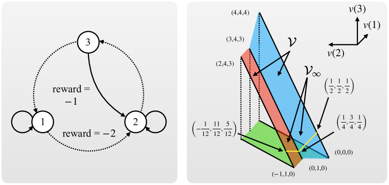
Figure 2: Illustration example. Left: the example MDP. There are three states marked by three circles respectively. There are two actions solid and dashed, both have deterministic effects. Taking action solid at state 3 results in a reward of $-1$. Taking action dashed at state 1 results in a reward of $-2$. All other rewards are $0$. Right: a graphical explanation of $\mathcal{V},\mathcal{V}_{\infty}$. The two yellow line segments together represent the solution set $\mathcal{V}_{\infty}$, which is not convex. The red and blue regions together represent $\mathcal{V}$.

Let $f(q)=\sum_{s,a}q(s,a)$. Such a choice of $f$ satisfies the assumption on $f$ in Theorem 5. Then by definition, for any $v\in\mathcal{V}_{\infty}$, we have

$$f(\tilde{r}+\tilde{P}v)=\hat{r}_{*}.$$

For the three-state MDP considered here, $\hat{r}_{*}=0$.

$$f(\tilde{r}+\tilde{P}v) =\sum_{s,a}r(s,a)+p(s^{\prime}\mid s,a)v(s^{\prime})$$

$$=-3+2v(1)+3v(2)+v(3).$$

Therefore,

$$2v(1)+3v(2)+v(3)=3.$$

In addition to the above equality, $\mathcal{V}_{\infty}$ needs to satisfy the state-value optimality equation (Equation 23). Therefore for any $v\in\mathcal{V}_{\infty}$,

$$v(1) =\max(v(1),-2+v(2)),$$

$$v(2) =\max(v(2),v(3)),$$

$$v(3) =\max(v(1),-1+v(2)),$$

which implies

$$v(1) \geq-2+v(2),$$

$$v(2) \geq v(3),$$

$$v(3) =\max(v(1),-1+v(2)).$$

Therefore

$$\mathcal{V}_{\infty}=\{v\in\mathbb{R}^{3}\mid v(1)\geq-2+v(2);v(2)\geq v(3);v(3)=\max(v(1),-1+v(2));$$

$$2v(1)+3v(2)+v(3)=3\}.$$

Graphically, $\mathcal{V}_{\infty}$ corresponds to the two connected yellow line segments in the right sub-figure in Figure 2. From the figure, we see that $\mathcal{V}_{\infty}$ is not convex.

Let $s$ and $d$ denote solid and dashed respectively. Consider any $q\in\mathcal{Q}_{\infty}$, in view of equation 22,

$$q(1,s)+q(1,d)+q(2,s)+q(2,d)+q(3,s)+q(3,d)=0.$$

In addition to the above equality, $\mathcal{Q}_{\infty}$ needs to satisfy the action-value optimality equation (Equation 2). Therefore for any $q\in\mathcal{Q}_{\infty}$,

$$q(1,s) =0-0+\max(q(1,s),q(1,d))$$

$$q(1,d) =-2-0+\max(q(2,s),q(2,d))$$

$$q(2,s) =0-0+\max(q(2,s),q(2,d))$$

$$q(2,d) =0-0+\max(q(3,s),q(3,d))$$

$$q(3,s) =-1-0+\max(q(2,s),q(2,d))$$

$$q(3,d) =0-0+\max(q(1,s),q(1,d)),$$

which implies

$$q(1,s) \geq q(1,d)$$

$$q(1,d) =-2+\max(q(2,s),q(2,d))$$

$$q(2,s) \geq q(2,d)$$

$$q(2,d) =\max(q(3,s),q(3,d))$$

$$q(3,s) =-1+\max(q(2,s),q(2,d))$$

$$q(3,d) =\max(q(1,s),q(1,d))$$

Consider two solutions $q_{1},q_{2}\in\mathcal{Q}_{\infty}$ defined as follows:

$$q_{1}(1,s) =\frac{1}{2},q_{1}(1,d)=-\frac{3}{2},$$

$$q_{1}(2,s) =\frac{1}{2},q_{1}(2,d)=\frac{1}{2},$$

$$q_{1}(3,s) =-\frac{1}{2},q_{1}(3,d)=\frac{1}{2},$$

$$q_{2}(1,s) =-\frac{2}{3},q_{2}(1,d)=-\frac{2}{3},$$

$$q_{2}(2,s) =\frac{4}{3},q_{2}(2,d)=\frac{1}{3},$$

$$q_{2}(3,s) =\frac{1}{3},q_{2}(3,d)=-\frac{2}{3}.$$

The midpoint of $q_{1}$ and $q_{2}$, $\bar{q}\doteq 0.5q_{1}+0.5q_{2}$, satisfies

$$\bar{q}(1,s) =-\frac{1}{12},\bar{q}(1,d)=-\frac{13}{12},$$

$$\bar{q}(2,s) =\frac{11}{12},\bar{q}(2,d)=\frac{5}{12},$$

$$\bar{q}(3,s) =-\frac{1}{12},\bar{q}(3,d)=-\frac{1}{12}.$$

Note that

$$\frac{5}{12}=\bar{q}(2,d)\neq\max(\bar{q}(3,s),\bar{q}(3,d))=-\frac{1}{12}.$$

Therefore $\bar{q}$ does not satisfy the action-value optimality equation (equation 2) and $\bar{q}\not\in\mathcal{Q}_{\infty}$. Thus $\mathcal{Q}_{\infty}$ is not convex.

A.6 General RVI Q

We now start to present the General RVI Q algorithm.

Let $\mathcal{I}\doteq\{1,2,\cdots,k\}$ where $k$ is a positive integer. Consider solving $\bar{r}\in\mathbb{R}$ and $q\in\mathbb{R}^{{\left\lvert\mathcal{I}\right\rvert}}$ in following equation

$$r(i)-\bar{r}+g(q)(i)-q(i)=0,\forall\ i\in\mathcal{I}$$ (38)

where $r\in\mathbb{R}^{\left\lvert\mathcal{I}\right\rvert}$ is any fixed ${\left\lvert\mathcal{I}\right\rvert}$-dim vector, and $g:\mathbb{R}^{{\left\lvert\mathcal{I}\right\rvert}}\to\mathbb{R}^{{\left\lvert\mathcal{I}\right\rvert}}$ satisfies 6.

We now consider an algorithm solving equation 38. This algorithm maintains an ${\left\lvert\mathcal{I}\right\rvert}$-dim vector of estimates $Q\in\mathbb{R}^{{\left\lvert\mathcal{I}\right\rvert}}$, and updates $Q$ using

$$Q_{n+1}(i) \doteq Q_{n}(i)+\alpha_{\nu(n,i)}\big{(}R_{n}(i)-F_{n}(Q_{n})+G_{n}(Q_{n})(i)-Q_{n}(i)+\epsilon_{n}(i)\big{)}I\{i\in Y_{n}\},$$ (39)

where

1. $\{Y_{n}\}$ is the “update schedule” – it is a set-valued process taking values in the set of nonempty subsets of $\mathcal{I}$ with the interpretation: $Y_{n}=\{i:i\textsuperscript{th}$ component of $Q$ was updated at time $n\}$,

2. $\nu(n,i)\doteq\sum_{k=0}^{n}\mathbf{I}\{i\in Y_{k}\}$, where $\mathbf{I}$ is the indicator function (i.e., $\nu(n,i)=$ the number of times the $i$ component was updated up to step $n$)

3. $\{\alpha_{n}\}$ is a step-size sequence,

4. $\{R_{n}\}$ is a sequence of i.i.d. random vectors satisfying $\mathbb{E}\left[R_{n}\right]=r,\forall\ n=0,1,\dots$,

5. for any $Q\in\mathbb{R}^{{\left\lvert\mathcal{I}\right\rvert}}$, $\{G_{n}(Q)\}$ is a sequence of i.i.d. random vectors satisfying $\mathbb{E}[G_{n}(Q)(i)]=g(Q)(i),\forall\ i\in\mathcal{I},n=0,1,\dots$,

6. for any $Q\in\mathbb{R}^{{\left\lvert\mathcal{I}\right\rvert}}$, $\{F_{n}(Q)\}$ is a sequence of i.i.d. random variables satisfying $\mathbb{E}[F_{n}(Q)]=f(Q),\forall\ n=0,1,\dots$ where $f:\mathcal{I}\to\mathbb{R}$ is a function satisfying 5,

7. $\epsilon_{n}$ is a sequence of random vectors of size ${\left\lvert\mathcal{I}\right\rvert}$.

We need the following assumptions in addition to Assumptions 2–5.

Assumption 6.

1) $g$ is a max-norm non-expansion, 2) $g$ is a span-norm non-expansion, 3) $g(x+ce)=g(x)+ce$ for any $c\in\mathbb{R},x\in\mathbb{R}^{{\left\lvert\mathcal{I}\right\rvert}}$, 4) $g(cx)=cg(x)$ for any $c\in\mathbb{R},x\in\mathbb{R}^{{\left\lvert\mathcal{I}\right\rvert}}$.

Let

$$M_{n+1}\doteq R_{n}-r+G_{n}(Q_{n})-g(Q_{n})-(F_{n}(Q_{n})-f(Q_{n}))e.$$ (40)

Let $\mathcal{F}_{n}\doteq\sigma(Q_{0},\epsilon_{0},M_{1},\epsilon_{1},M_{2},\dots,\epsilon_{n-1},M_{n})$ be the increasing family of $\sigma$-fields. By the above construction, $\{M_{n+1}\}$ is a martingale difference sequence w.r.t. $\mathcal{F}_{n}$. That is $\mathbb{E}[M_{n+1}\mid\mathcal{F}_{n}]=0$ a.s., $n\geq 0$.

Assumption 7.

For $n\in\{0,1,2,\dots\}$, $\mathbb{E}[\left\lVert R_{n}-r\right\rVert^{2}\mid\mathcal{F}_{n}]\leq K$, $\mathbb{E}[\left\lVert G_{n}(Q)-g(Q)\right\rVert^{2}\mid\mathcal{F}_{n}]\leq K(1+\left\lVert Q\right\rVert^{2})$ for any $Q\in\mathbb{R}^{\left\lvert\mathcal{I}\right\rvert}$, and $\mathbb{E}[\left\lVert F_{n}(Q)-f(Q)e\right\rVert^{2}\mid\mathcal{F}_{n}]\leq K(1+\left\lVert Q\right\rVert^{2})$ for any $Q\in\mathbb{R}^{\left\lvert\mathcal{I}\right\rvert}$ for a suitable constant $K>0$.

We make the following assumption on $\epsilon_{n}$.

Assumption 8.

$\mathbb{E}[\left\lVert\epsilon_{n}\right\rVert^{2}\mid\mathcal{F}_{n}]<K(1+\left\lVert Q_{n}\right\rVert^{2})$ a.s.. Further, $\epsilon_{n}$ converges to 0 a.s..

Assumption 9.

Equation 38 has a unique solution of $\bar{r}$. That is, there exists a pair $\bar{r}\in\mathbb{R},q\in\mathbb{R}^{\left\lvert\mathcal{I}\right\rvert}$ satisfying equation 38 and if both $\bar{r}_{1},q_{1}$ and $\bar{r}_{2},q_{2}$ are solutions equation 38, $\bar{r}_{1}=\bar{r}_{2}$.

Denoted the unique solution of $\bar{r}$ by $r_{\#}$.

Define $\mathcal{Q}_{\#}$ to be the set of $q\in\mathbb{R}^{{\left\lvert\mathcal{I}\right\rvert}}$ satisfying equation 38 and

$$r_{\#} =f(q).$$ (41)

Assumption 10.

$\mathcal{Q}_{\#}$ is non-empty, bounded, closed, and connected.

Assumption 11.

If $r(i)=0,\forall\ i\in\mathcal{I}$, then $0$ is the only element in $\mathcal{Q}_{\#}$.

1 is assumed in Section 2 of Wan et al. (2021b). Assumptions 2–8 are the same as Assumptions A.1-A.7 by Wan et al. (2021b). Assumptions 9–11 replace Assumption A.8 by Wan et al. (2021b).

Theorem 6.

Under Assumptions 2-11, General RVI Q (equation 39) converges, almost surely, $Q_{n}$ to $\mathcal{Q}_{\#}$ and $f(Q_{n})$ to $r_{\#}$.

Proof.

The proof would by a large degree repeats that of Theorem A.1 by Wan et al. (2021). For simplicity, we only highlight modifications.

Both our proof and the proof of Theorem A.1 study two ordinary differential equations (ODEs):

$$\dot{y}_{t} \doteq T_{1}(y_{t})-y_{t},$$ (42)

$$\dot{x}_{t} \doteq T_{2}(x_{t})-x_{t}=T_{1}(x_{t})-x_{t}+\left(r_{\#}-f(x_{t})\right)e,$$ (43)

where

$$T_{1}(Q)(i) \doteq r(i)+g(Q)(i)-r_{\#},$$

$$T_{2}(Q)(i) \doteq r(i)+g(Q)(i)-f(Q)$$

$$=T_{1}(Q)(i)+\left(r_{\#}-f(Q)\right).$$

Lemmas A.1 and A.3 by Wan et al. (2021) and their proofs still hold (by replacing $r_{\infty}$ with $r_{\#}$). Lemma A.2 by Wan et al. (2021) is replaced by the following one. The proof follows the same arguments as those for Lemma A.2.

Lemma 5.

The set of equilibrium points of equation 43 is $\mathcal{Q}_{\#}$.

Lemma A.4 by Wan et al. (2021) is replaced with the following two lemmas.

Lemma 6.

If $r(i)=0,\forall\ i\in\mathcal{I}$, $0$ is the globally asymptotically stable equilibrium for equation 43.

Proof.

We have assumed that $0$ is the only element in $\mathcal{Q}_{\#}$ in Assumption 11 and $0$ is thus the unique equilibrium of equation 43. The rest follows the proof of Lemma A.4 by Wan et al. (2021) by replacing $q_{\infty}$ with $0$. ∎

Lemma 7.

$\mathcal{Q}_{\#}$ is a compact connected internally chain transitive invariant set for the ODE equation 43. Furthermore, any set that contains points not in $\mathcal{Q}_{\#}$ is not a compact connected internally chain transitive invariant set for the ODE equation 43.

Proof.

According to Assumption 10, $\mathcal{Q}_{\#}$ is closed and bounded and is thus compact. Assumption 10 also assumes that $\mathcal{Q}_{\#}$ is connected. $\mathcal{Q}_{\#}$ is an internally chain transitive invariant set for the ODE equation 43 because every element in $\mathcal{Q}_{\#}$ is an equilibrium point of the ODE and $\mathcal{Q}_{\#}$ is connected.

If a set contains a point $x\in\mathbb{R}^{|\mathcal{I}|}$ that is not in $\mathcal{Q}_{\#}$, this set can not be internally chain transitive because $x$ is "transient" and the trajectory of equation 43 can not be arbitrarily close to $x$ at some arbitrarily large time step. ∎

The last step is to show convergence of a synchronous version of equation 39

$$Q_{n+1}(i) \doteq Q_{n}(i)+\alpha_{\nu(n,i)}\big{(}R_{n}(i)-F_{n}(Q_{n})+G_{n}(Q_{n})(i)-Q_{n}(i)+\epsilon_{n}(i)\big{)}.$$ (44)

This result, together with Assumptions 3 and 4, guarantees convergence of the asynchronous update (equation 44) by applying results from Section 7.4 by Borkar (2009)

Lemma 8.

Equation 44 converges a.s. $Q_{n}$ to $\mathcal{Q}_{\#}$ as $n\to\infty$.

Proof.

The proof essentially follows that of Lemma A.5 with two changes. First, using Lemma 6 we can show that the ODE $\dot{x}_{t}=h_{\infty}(x_{t})=g(x_{t})-f(x_{t})e-x_{t}$ has the origin as the unique globally asymptotically stable equilibrium. Second, the proof of Lemma A.5 uses Borkar’s (2009) Theorem 2, which proves that $Q_{n}$ converges to a (possibly sample path dependent) compact connected internally chain transitive invariant set of $\dot{x}_{t}=h(x_{t})$ where

$$h(Q_{n})(i) \doteq r(i)-f(Q_{n})+g(Q_{n})(i)-Q_{n}(i).$$

Lemma 7 and Theorem 2 by Borkar (2009) together imply that $Q_{n}$ must converge to $\mathcal{Q}_{\#}$. ∎

∎

A.7 Verifying 9–11

When casting General RVI Q to RVI Q-learning, equation 38 becomes equation 2. It is then clear that 9 satisfies because the associated MDP is communicating, 10 holds because of Theorem 5 and 11 holds because of Lemma 3.

When casting General RVI Q to Differential Q-learning, equation 38 becomes equation 2 for an MDP with the same transition dynamics as the original one and all rewards being shifted by a constant that depends on initial action-value estimate $Q_{0}$ and reward rate estimate $\bar{R}_{0}$. It is clear that this new MDP, just like the original one, is communicating. Therefore Theorem 5 and Lemma 3 hold and thus 9–11 hold.

When casting General RVI Q to inter-option Differential Q-learning, equation 38 becomes equation 4 for an SMDP with the same transition dynamics as the original one and the reward of each state-option pair being shifted in proportional to its expected duration. Again the resulting SMDP is communicating and therefore Theorem 5 and Lemma 3 hold and thus 9–11 hold.

When casting General RVI Q to intra-option Differential Q-learning, equation 38 becomes equation 5, which is the same as equation 4 by Proposition 2 for the reward shifted SMDP introduced in the previous paragraph.

A.8 Convergence of Reward Rates of Greedy Policies

Lemma 9.

Assume that the SMDP is weakly communicating, suppose $Q_{n}$ converges to $\mathcal{Q}_{\infty}$ almost surely, let $\pi_{n}$ be a greedy policy w.r.t. $Q_{n}$, $r(\pi_{n},s)\to\hat{r}_{*}$ almost surely.

Proof.

We will need the following lemma for the proof.

Lemma 10.

For any $m\in\{1,2,3,\ldots\}$, $a,b\in\mathbb{R}^{m}$, $b>0$, and for any $p\in\mathbb{R}^{m}$ such that $p\geq 0$, $\sum_{s}p(s)=1$,

$$\frac{p^{\top}a}{p^{\top}b} \geq\min_{s}\frac{a(s)}{b(s)},$$

$$\frac{p^{\top}a}{p^{\top}b} \leq\max_{s}\frac{a(s)}{b(s)}.$$

Proof.

For any $s\in\{1,2,3,\ldots,m\}$

$$\frac{a(s)}{b(s)} \geq\min_{s^{\prime}}\frac{a(s^{\prime})}{b(s^{\prime})}$$

$$a(s) \geq b(s)\min_{s^{\prime}}\frac{a(s^{\prime})}{b(s^{\prime})}$$

$$p(s)a(s) \geq p(s)b(s)\min_{s^{\prime}}\frac{a(s^{\prime})}{b(s^{\prime})}$$

Therefore

$$p^{\top}a \geq p^{\top}b\min_{s^{\prime}}\frac{a(s^{\prime})}{b(s^{\prime})}$$

By our assumptions on $b$ and $p$, $p^{\top}b>0$, we have

$$\frac{p^{\top}a}{p^{\top}b} \geq\min_{s^{\prime}}\frac{a(s^{\prime})}{b(s^{\prime})}.$$

$\frac{p^{\top}a}{p^{\top}b}\leq\max_{s}\frac{a(s)}{b(s)}$ can be shown in the same way. ∎

Given that $Q_{n}$ converges to $\mathcal{Q}_{\infty}$, consider $r(\pi_{n},s)$ where $\pi_{n}$ is a greedy policy w.r.t. $Q_{n}$. We show that $r(\pi_{n},s)$ converges to $\hat{r}_{*}$ for all $s\in\mathcal{S}$.

For any $\pi\in\hat{\Pi}$, let $P_{\pi}$ denote the ${\left\lvert\mathcal{S}\right\rvert}\times{\left\lvert\mathcal{O}\right\rvert}\times{\left\lvert\mathcal{S}\right\rvert}\times{\left\lvert\mathcal{O}\right\rvert}$ transition probability matrix under policy $\pi$. That is,

$$P_{\pi}(s,o,s^{\prime},o^{\prime})\doteq\sum_{r,l}\hat{p}(s^{\prime},r,l\mid s,o)\pi(o^{\prime}\mid s^{\prime}).$$ (45)

Let $P_{\pi}^{\infty}$ be the limiting matrix of $P_{\pi}$, which is the Cesaro limit of the sequence $\{P_{\pi}^{i}\}_{i=1}^{\infty}$:

$$P_{\pi}^{\infty}\doteq\lim_{n\to\infty}\frac{1}{n}\sum_{i=0}^{n-1}P_{\pi}^{i}.$$

Because $\mathcal{S}$ is finite, the Cesaro limit exists and $P_{\pi}^{\infty}$ is a stochastic matrix (has row sums equal to 1).

Let $r(s,o)\doteq\sum_{s^{\prime},r,l}\hat{p}(s^{\prime},r,l\mid s,o)r$ be the one-stage option reward and $l(s,o)\doteq\sum_{s^{\prime},r,l}\hat{p}(s^{\prime},r,l\mid s,o)l$ be the one-stage option length. Let $r(\pi,s,o)\doteq\sum_{s^{\prime},r,l}\hat{p}(s^{\prime},r,l\mid s,o)r(\pi,s^{\prime})$ be the reward rate of policy $\pi$ starting from $s,o$. By part (a) of Theorem 11.4.1 in Puterman (1994),

$$r(\pi_{n},s,o)=\frac{P_{\pi_{n}}^{\infty}r(s,o)}{P_{\pi_{n}}^{\infty}l(s,o)}.$$

Thus we have,

$$r(\pi_{n},s,o) =\frac{P_{\pi_{n}}^{\infty}r(s,o)}{P_{\pi_{n}}^{\infty}l(s,o)}$$

$$=\frac{P_{\pi_{n}}^{\infty}(r+P_{\pi_{n}}Q_{n}-Q_{n})(s,o)}{P_{\pi_{n}}^{\infty}l(s,o)}$$

$$\geq\min_{s^{\prime},o^{\prime}}\frac{(r+P_{\pi_{n}}Q_{n}-Q_{n})(s^{\prime},o^{\prime})}{l(s^{\prime},o^{\prime})}$$

$$=\min_{s^{\prime},o^{\prime}}\frac{(TQ_{n}-Q_{n})(s^{\prime},o^{\prime})}{l(s^{\prime},o^{\prime})},$$

where the inequality holds because of Lemma 10, and $TQ_{n}(s,o)\doteq r(s,o)+\sum_{s^{\prime},r,l}\hat{p}(s^{\prime},r,l\mid s,o)\max_{o^{\prime}}Q_{n}(s^{\prime},o^{\prime})$.

Because the SMDP is weakly communicating, consider a deterministic optimal policy $\pi\in\hat{\Pi}_{*}$, $r(\pi,s)=\hat{r}_{*},\forall\ s\in\mathcal{S}$. Therefore $r(\pi,s,o)=\hat{r}_{*}$. Now we have, for any $s,o$,

$$\hat{r}_{*} =r(\pi,s,o)$$

$$=\frac{P_{\pi^{*}}^{\infty}r(s,o)}{P_{\pi^{*}}^{\infty}l(s,o)}$$

$$=\frac{P_{\pi^{*}}^{\infty}(r+P_{\pi}Q_{n}-Q_{n})(s,o)}{P_{\pi^{*}}^{\infty}l(s,o)}$$

$$\leq\max_{s^{\prime},o^{\prime}}\frac{(r+P_{\pi}Q_{n}-Q_{n})(s^{\prime},o^{\prime})}{l(s^{\prime},o^{\prime})}$$

$$\leq\max_{s^{\prime},o^{\prime}}\frac{(r+P_{\pi_{n}}Q_{n}-Q_{n})(s^{\prime},o^{\prime})}{l(s^{\prime},o^{\prime})}$$

$$=\max_{s^{\prime},o^{\prime}}\frac{(TQ_{n}-Q_{n})(s^{\prime},o^{\prime})}{l(s^{\prime},o^{\prime})}.$$

The first inequality holds because of Lemma 10 and the second inequality holds because $\pi_{n}$ is a greedy policy w.r.t. $Q_{n}$.

With the above results, and that $\hat{r}_{*}\geq r(\pi_{n},s,o)$, we have, for any $s,o$,

$$\min_{s^{\prime},o^{\prime}}\frac{(TQ_{n}-Q_{n})(s^{\prime},o^{\prime})}{l(s^{\prime},o^{\prime})}\leq r(\pi_{n},s,o)\leq\hat{r}_{*}\leq\max_{s^{\prime},o^{\prime}}\frac{(TQ_{n}-Q_{n})(s^{\prime},o^{\prime})}{l(s^{\prime},o^{\prime})}$$

Therefore,

$$\max_{s,o}\hat{r}_{*}-r(\pi_{n},s,o)\leq sp\left(\frac{TQ_{n}-Q_{n}}{l}\right),$$

where $sp(x)=\max_{i}x(i)-\min x(i)$ denotes the span of vector $x$.

Because $Q_{n}\to\mathcal{Q}_{\infty}$ a.s., every point $q$ in $\mathcal{Q}_{\infty}$ satisfies $sp((Tq-q)/l)=0$ because $(Tq-q)/l=\hat{r}_{*}e$ by equation 4. In addition, $sp((TQ_{n}-Q_{n})/l)$ is a continuous function of $Q_{n}$, by continuous mapping theorem, $sp((TQ_{n}-Q_{n})/l)\to 0$ a.s.. Therefore we conclude that $r(\pi_{n},s,o)\to\hat{r}_{*},\forall s,o$. By definition, $r(\pi_{n},s)=\sum_{o}\pi_{n}(o\mid s)r(\pi_{n},s,o)$. Therefore $r(\pi_{n},s)\to\hat{r}_{*}$ ∎

Appendix B Empirical Results

In this section, we empirically verify our convergence results of Differential Q-learning and RVI Q-learning by showing the dynamics of estimated action values of the two algorithms in a communicating MDP and a weakly communicating MDP.

We first consider the communicating MDP shown at the bottom of Figure 1. For this MDP, we apply Differential Q-learning with initial action values $0$, initial reward rate estimate $-3$, and $\eta=1$. The behavior policy chooses action solid with probability $0.8$ and action dashed with probability $0.2$ for both two states. The stepsize is $0.1$. We performed 10 runs for each algorithm. Each run starts from state 1 and lasts for $1000$ steps. Every 10 steps, we recorded the estimated action values and plotted the higher action value for each state in the figure. Figure 4(left) shows the evolution of these action values. In the right panel of the same figure, we also show it using RVI Q-learning with action values being initialized with $0$ and $f(q)=q(1,\texttt{dashed})$. A more detailed explanation is provided in the figure’s caption. It can be seen that for both algorithms, 1) for each run, the estimated action-value function converged to a point in the solution set (the black line segments), and 2) for different runs, the estimated action values generally converged to different points in the solution set.

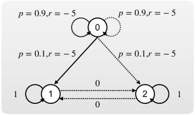
Figure 3: A weakly communicating MDP modified from the communicating MDP shown at the bottom of Figure 1 by adding a transient state $0$.

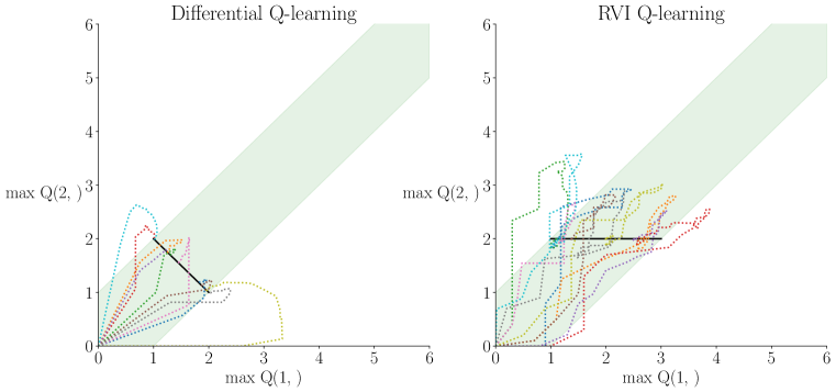
Figure 4: Evolution of estimated action values of Differential Q-learning and RVI Q-learning in the communicating MDP shown at the bottom of Figure 1. In each figure, the $x$ and $y$ axes are the higher estimated action value at state $1$ and $2$, respectively. The light green region marks the solution set of the action-value optimality equation (Equation 2), and the black line segment marks the solution set $\mathcal{Q}_{\infty}$. Each colored dotted trajectory marks the evolution of the estimated action values. Each trajectory starts from zero point and ends at some point on the black line segment.

We also applied both of the two algorithms, with the same parameter settings and initialization in a weakly communicating MDP (Figure 3), which is just the communicating MDP plus a transient state. In the transient state, taking both solid and dashed actions stays at the transient state with probability $0.9$. The MDP moves to state 1 with probability $0.1$ given action solid and to state 2 with probability $0.1$ given action dashed. The reward starting from state 0 is always $-5$. The starting state is $0$. Because the agent could spend different amounts of time in the transient state for different runs, the agent may enter the communicating set, which contains states 1 and 2, with different action values associated with state $0$.

The solution set of Differential Q-learning depends on the action values associated with the transient states when entering the communicating class. Therefore in the figure, the points that the estimated action-value function converged to, corresponding to different runs, are not in a line. Nevertheless, the estimated action-value function in all runs converged to the green region, which corresponds to the solution set of the action-value optimality equation.

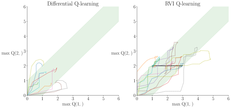
Figure 5: Evolution of estimated action values of Differential Q-learning and RVI Q-learning in the weakly communicating MDP shown in Figure 3.

On the other hand, The solution set of RVI Q-learning with the choice of the reference function $f(q)=q(1,\texttt{dashed})$ does not depend on the action values associated with states in the communicating class when entering the class. Therefore the solution set did not vary across different runs. Note that if we chose $f(q)=q(0,\texttt{dashed})$, then again the solution set of RVI Q-learning has that dependence.

Appendix C Gosavi’s (2004) Convergence Result Is Incorrect

The convergence result of Gosavi’s proposed algorithm is presented in Theorem 2 of his paper. In the proof of the theorem, they used Borkar’s two-time scale stochastic approximation result to prove the convergence of the proposed algorithm. Specifically, they argued that their algorithm is a special case of the general class of algorithms considered in Borkar’s result. As Gosavi quotes, "Note that the Eqs. (48) and (49) for SMDPs form a special case of the general class of algorithms (29) and (30) analyzed using the lemma given in Section 5.1.1. " However, a closer look at these equations shows that equation (49) is not a special case of equation (30). Note that because $\rho^{k}$ is a scalar, $y^{k}$ only has one element and thus the $f$ function in equation (30) does not vary across different state-option pairs. However, this is not true for the $f$ function in equation (49). It appears to us that there is no simple fix for this issue.