Low-Dose CT Using Denoising Diffusion Probabilistic Model for 20$\times$ Speedup

Abstract

Low-dose computed tomography (LDCT) is an important topic in the field of radiology over the past decades. LDCT reduces ionizing radiation-induced patient health risks but it also results in a low signal-to-noise ratio (SNR) and a potential compromise in the diagnostic performance. In this paper, to improve the LDCT denoising performance, we introduce the conditional denoising diffusion probabilistic model (DDPM) and show encouraging results with a high computational efficiency. Specifically, given the high sampling cost of the original DDPM model, we adapt the fast ordinary differential equation (ODE) solver for a much-improved sampling efficiency. The experiments show that the accelerated DDPM can achieve 20x speedup without compromising image quality.

1 Introduction

Computed tomography (CT) plays an indispensable role in radiology due to its high-contrast resolution, fast imaging speed, and many utilities. With the increasing popularity of CT scans, there is a major safety concern on ionizing radiation from x-ray exposure to the patient. To reduce the x-ray radiation-induced risks during a CT scan, low-dose CT (LDCT) research has attracted a widespread attention so that the image quality of LDCT can be optimized despite the radiation dose reduction.

To solve the above challenge of LDCT, there have been numerous efforts made in the past few decades. A natural approach for LDCT is to post-process a noisy LDCT image. Inspired by established methods for natural image denoising, non-local means (NLM) and block-matching 3D (BM3D) were adapted for LDCT denoising li2014adaptive ; feruglio2010block ; kang2013image , significantly improving the LDCT performance. Although these post-processing methods do remove LDCT image noise, the resultant image quality often hardly meets the clinical requirements, since it is difficult to model the noise contained in the LDCT images, and thus new artifacts can be frequently introduced. Another commonly used LDCT denoising approach is referred to as model-based iterative reconstruction (MBIR), which is to establish a data model in the projection domain and a content model in the image domain, and then minimize an objective function for model fitting iteratively. Especially, inspired by compressed sensing (CS) theory, the regularization model with total variation (TV) greatly improves the reconstruction quality yu2005total . Subsequently, many methods were proposed to solve the over-smoothness problem associated with TV minimization, including anisotropic TV chen2013limited , total generalized variation (TGV) niu2014sparse , fractional order TV zhang2014few ; zhang2016statistical , and so on. In addition to the TV regularization, other effective priors were also formulated, such as NLM chen2009bayesian , tight framework gao2011multi , low-rank cai2014cine , dictionary learning xu2012low ; chen2013improving , learned sparsifying transform zheng2016low , etc. These regularization-based methods can achieve a promising denoising performance by careful designing the regularization term and fine-tuning the hyperparameters. However, that means extensive experience and skills, and limited clinical applications.

With the recent development of the deep learning (DL) techniques lecun2015deep , LDCT denoising was immediately identified as an earliest application target wang2016perspective . Chen et al. first published a convolutional neural network (CNN) for LDCT denoising and achieved remarkable performance chen2017lowdose . Progress in this area has been rapid, including residual structures to improve both the training convergence and denoising performance chen2017low ; jin2017deep ; kang2017deep ; han2018framing , and incorporate various loss functions and training strategies, such as adversarial loss wolterink2017generative ; yang2018low , perceptual loss yang2018low , edge incoherence loss shan2019competitive , etc. Also, in some studies DL and MBIR algorithms were combined for synergies wu2017iterative ; chen2018learn ; adler2018learned ; gupta2018cnn ; chun2020momentum ; xiang2021fista . These methods deploy CNNs in iterative optimization schemes so that the priors and penalty parameters can be learned in a data-driven fashion.

Very recently, the denoising diffusion probabilistic model (DDPM) sohl2015deep ; ho2020denoising ; croitoru2022diffusion ; yang2022diffusion emerged as a generative model with the mode diversity and output quality superior to that of the generative adversarial network (GAN) goodfellow2020generative ; adler2018learned ; sohl2015deep ; ho2020denoising ; song2019generative ; song2020score ; dhariwal2021diffusion ; nichol2021improved . DDPM gradually perturbs an original data distribution until into a standard distribution, typically a normal distribution. Then, DDPM iteratively recovers the data distribution in a learned reverse diffusion process. Song et al. interpreted the forward and backward diffusion processes in the stochastic differential equation (SDE) framework song2020score . The SDE-based diffusion model allows the learning of the reverse diffusion process in continuous time, and has been applied to a variety of tasks, such as image super-resolution rombach2022high ; saharia2022image , image inpainting lugmayr2022repaint , image editing meng2021sdedit , image translation choi2021ilvr ; saharia2022palette , and so on.

In this paper, we introduce a conditional DDPM for LDCT denoising. The U-Net ho2020denoising is adopted to learn the reverse diffusion process of a normal-dose CT (NDCT) image conditioned on a LDCT counterpart. Then, by gradually sampling, cleaner images can be step by step recovered from a normal noise distribution under the condition of the LDCT image. The final image generated by DDPM can remove structural noise in the input LDCT image while preserving clinically important details. However, the sampling efficiency of the original DDPM model is low and can hardly meet clinical requirements. To alleviate this problem, here we use a fast ordinary differential equation (ODE) solver lu2022dpm for a much-boosted efficient sampling, 20 $\times$ faster than that of the original DDPM.

2 Methodology

2.1 Supervised Deep LDCT Denoising

Currently, a typical DL-based LDCT denoising method trains a network to learn a mapping from LDCT images to NDCT images. Let us assume that $\bm{x}\in\mathbb{R}^{N}$ and $\bm{y}\in\mathbb{R}^{N}$ are paired LDCT and NDCT images, then the parameters of the network can be trained as follows:

$$\min_{\bm{\theta}}\left\|D_{\bm{\theta}}(\bm{x})-\bm{y}\right\|_{2}^{2},$$ (1)

where $D_{\bm{\theta}}:\mathbb{R}^{N}\rightarrow\mathbb{R}^{N}$ is the network defined by $\bm{\theta}$, which is a vector of parameters.

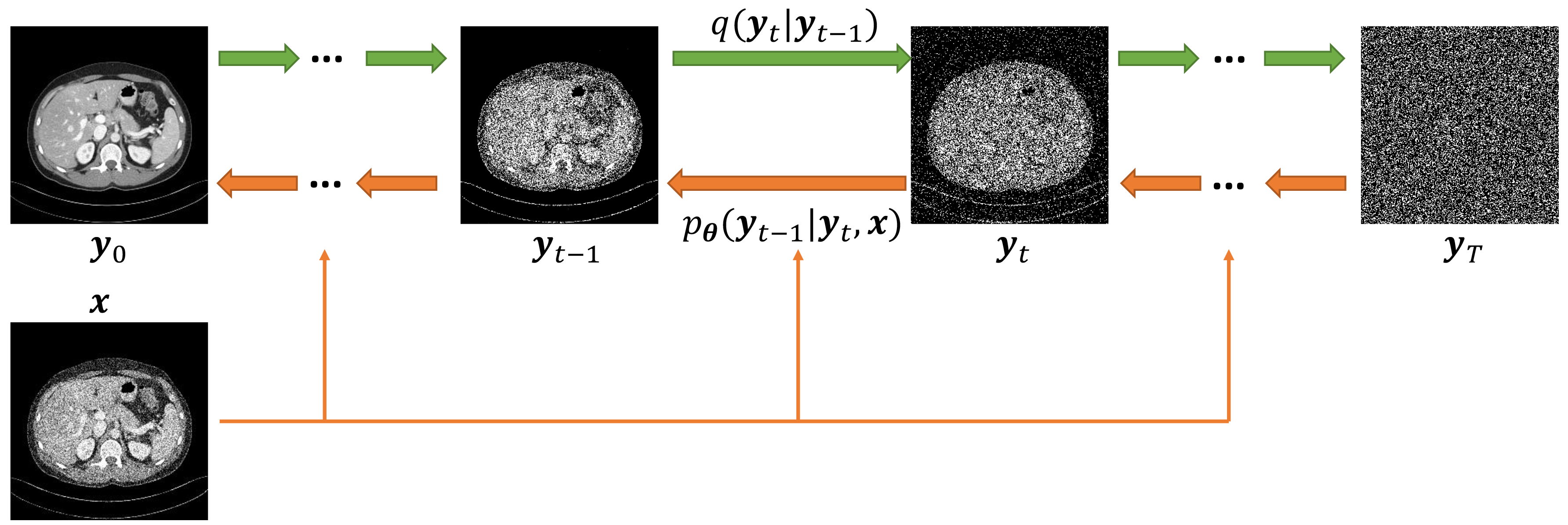
Figure 1: Conditional DDPM for LDCT denoising, trained in the supervised mode.

2.2 Conditional DDPM for LDCT Denoising

As shown in Fig. 1, the conditional DDPM for LDCT denoising consists of a forward process and a reverse process. In reference to ho2020denoising , the forward process is defined as a Markov chain which gradually adds Gaussian noise to an NDCT image $\bm{y}_{0}$ according to a hyper-parameterized variance sequence $\beta_{1},\beta_{2},\cdots,\beta_{T}$:

$$q(\bm{y}_{1:T}|\bm{y}_{0})=\prod_{t=1}^{T}q(\bm{y}_{t}|\bm{y}_{t-1}),$$ (2)

where

$$q(\bm{y}_{t}|\bm{y}_{t-1})=\mathcal{N}(\bm{y}_{t}|\sqrt{1-\beta_{t}}\bm{y}_{t-1},\beta_{t}\bm{I}).$$ (3)

According to the properties of the Gaussian distribution, the sampling operation can be directly performed at an arbitrary timestep $t$ without any iteration:

$$q(\bm{y}_{t}|\bm{y}_{0})=\mathcal{N}(\bm{y}_{t}|\sqrt{\bar{\alpha}_{t}}\bm{y}_{0},(1-\bar{\alpha}_{t})\bm{I}),$$ (4)

where $\alpha_{t}=1-\beta_{t}$ and $\bar{\alpha}_{t}=\prod_{i=1}^{t}\alpha_{i}$. After the forward process, $\bm{y}_{T}$ will follow a standard normal distribution $\mathcal{N}(0,\bm{I})$ when $T$ is large enough. Then, it can be shown that the posterior distribution of $\bm{y}_{t-1}$ given $\bm{y}_{t}$ and $\bm{y}_{0}$ can be formulated as follows:

$$\left\{\begin{aligned} &q(\bm{y}_{t-1}|\bm{y}_{t},\bm{y}_{0})=\mathcal{N}(\bm{y}_{t-1}|\tilde{\mu}_{t}(\bm{y}_{t},\bm{y}_{0}),\sigma_{t}^{2}\bm{I}),\\ &\tilde{\mu}_{t}(\bm{y}_{t},\bm{y}_{0})=\frac{\sqrt{\alpha_{t}}(1-\bar{\alpha}_{t-1})}{1-\bar{\alpha}_{t}}\bm{y}_{t}+\frac{\sqrt{\bar{\alpha}_{t-1}}(1-\alpha_{t})}{1-\bar{\alpha}_{t}}\bm{y}_{0},\\ &\sigma_{t}^{2}=\frac{(1-\bar{\alpha}_{t-1})(1-\alpha_{t})}{1-\bar{\alpha}_{t}}.\end{aligned}\right.$$ (5)

Similar to the forward process, the reverse process conditioned on a LDCT image $\bm{x}$ is also a Markov chain defined by

$$p_{\theta}(\bm{y}_{0:T}|\bm{x})=p(\bm{y}_{T})\prod_{t=1}^{T}p_{\theta}(\bm{y}_{t-1}|\bm{y}_{t},\bm{x}),$$ (6)

where

$$p_{\theta}(\bm{y}_{t-1}|\bm{y}_{t},\bm{x})=\mathcal{N}(\bm{y}_{t-1}|\mu_{\theta}(\bm{y}_{t},\bm{x},t),\sigma_{t}^{2}\bm{I}),$$ (7)

where $\bm{y}_{T}$ is sampled from a standard normal distribution $p(\bm{y}_{T})\sim\mathcal{N}(0,\bm{I})$, $\mu_{\theta}$ is the expectation computed by a learned U-Net model ho2020denoising .

The neural network is trained with a variational lower bound (VLB) of the negative log-likelihood:

$$\mathcal{L}_{VLB}=\mathbb{E}_{q}\left[-\log\frac{p_{\theta}(\bm{y}_{0:T}|\bm{x})}{q(\bm{y}_{1:T}|\bm{y}_{0})}\right]\geq\mathbb{E}\left[-\log p_{\theta}(\bm{y}_{0}|\bm{x})\right].$$ (8)

After inserting the Gaussian density function into Eq. (8) and removing the constant, the objective function can be rewritten as

$$\mathcal{L}=\mathbb{E}_{\bm{x},\bm{y}}\mathbb{E}_{t}\left[\frac{1}{2\sigma_{t}^{2}}\left\|\tilde{\mu}_{t}(\bm{y}_{t},\bm{y}_{0})-\mu_{\theta}(\bm{y}_{t},\bm{x},t)\right\|_{2}^{2}\right].$$ (9)

Specifically, the forward process can be implemented as

$$\bm{y}_{t}=\sqrt{\bar{\alpha}_{t}}\bm{y}_{0}+\sqrt{1-\bar{\alpha}_{t}}\bm{\epsilon},\ \bm{\epsilon}\sim\mathcal{N}(0,\bm{I}),$$ (10)

Then, the posterior expectation in Eq. (5) can be rewritten as

$$\tilde{\mu}_{t}(\bm{y}_{t},\bm{y}_{0})=\tilde{\mu}_{t}\left(\bm{y}_{t},\frac{1}{\sqrt{\bar{\alpha}}}\left(\bm{y}_{t}-\sqrt{1-\bar{\alpha}}\bm{\epsilon}\right)\right)=\frac{1}{\sqrt{\bar{\alpha}}}\left(\bm{y}_{t}-\frac{1-\alpha_{t}}{\sqrt{1-\bar{\alpha}}}\bm{\epsilon}\right).$$ (11)

Instead of directly learning the expectation, the U-Net model $D_{\bm{\theta}}$ is trained to predict the noise vector $\bm{\epsilon}$. Then, the objective function Eq. (9) becomes

$$\mathcal{L}=\mathbb{E}_{\bm{x},\bm{y}}\mathbb{E}_{\bm{\epsilon},t}\left[\frac{(1-\alpha_{t})^{2}}{2\sigma_{t}^{2}\bar{\alpha}(1-\bar{\alpha})}\left\|\bm{\epsilon}-D_{\bm{\theta}}(\sqrt{\bar{\alpha}_{t}}\bm{y}_{0}+\sqrt{1-\bar{\alpha}_{t}}\bm{\epsilon},\bm{x},t)\right\|_{2}^{2}\right].$$ (12)

According to ho2020denoising , we remove the weight of the $\ell_{2}$ norm for better training performance. Finally, for inference the sampling operation $\bm{y}_{t-1}\sim p_{\theta}(\bm{y}_{t-1}|\bm{y}_{t})$ can be computed as follows:

$$\bm{y}_{t-1}=\frac{1}{\sqrt{\bar{\alpha}}}\left(\bm{y}_{t}-\frac{1-\alpha_{t}}{\sqrt{1-\bar{\alpha}}}D_{\bm{\theta}}(\bm{y}_{t},\bm{x},t)\right)+\sigma_{t}\bm{z},\ \bm{z}\sim\mathcal{N}(0,\bm{I}).$$ (13)

For clarify, Algorithms 1 and 2 are presented in the pseudo codes for training and inference, respectively.

Input: Number of time steps $T$; Variance schedule $\{\beta_{t}|t=1,2,...,T\}$

Output: Trained model $D_{\bm{\theta}}$

Initialize $D_{\bm{\theta}}$ randomly;

while not converged do

       $(\bm{x},\bm{y}_{0})\sim p(\bm{x},\bm{y})$

      $t\sim\mathrm{Uniform}(\{1,2,...,T\})$

      $\bm{\epsilon}\sim\mathcal{N}(0,\bm{I})$

      Update $\bm{\theta}$ with the gradient $\nabla_{\theta}\left\|\bm{\epsilon}-D_{\bm{\theta}}(\sqrt{\bar{\alpha}_{t}}\bm{y}_{0}+\sqrt{1-\bar{\alpha}_{t}}\bm{\epsilon},\bm{x},t)\right\|_{2}^{2}$

end while

Algorithm 1 Training of the denoising model $D_{\bm{\theta}}$.

Input: Number of time steps $T$; Variance schedule $\{\beta_{t}|t=1,2,...,T\}$

Output: $\bm{y}_{0}$

Load $D_{\bm{\theta}}$;

$\bm{y}_{T}\sim\mathcal{N}(0,\bm{I})$

for $t=1,2,...,T$ do

       $\bm{z}\sim\mathcal{N}(0,\bm{I})$ if $t>1$ else $\bm{z}=0$

      $\bm{y}_{t-1}=\frac{1}{\sqrt{\bar{\alpha}}}\left(\bm{y}_{t}-\frac{1-\alpha_{t}}{\sqrt{1-\bar{\alpha}}}D_{\bm{\theta}}(\bm{y}_{t},\bm{x},t)\right)+\sigma_{t}\bm{z}$

end for

Algorithm 2 Inference with the trained denoising model $D_{\bm{\theta}}$.

2.3 Fast ODE Solver

Because the inference phase originally requires thousands of sampling steps, the computational cost is too expensive to meet clinical requirements. Therefore, it is necessary to accelerate the sampling process of DDPM. In song2020score , Song et al. proved that the reverse process of DDPM has a form equivalent to a probability flow ODE. Thus, the RK45 ODE solver dormand1980family can be applied to greatly reduce the number of sampling steps. In this study, we introduce a fast ODE solver to further improve the sampling efficiency.

To cast the discrete diffusion processes of DDPM in the continuous form, Kingma et al. kingma2021variational proved that the forward process for $t\in\{1,2,...,T\}$ following the distribution Eq. (4) is equivalent to a stochastic differential equation (SDE) starting from $\bm{y}_{0}\sim p(\bm{y}_{0})$ for any $t\in[0,T]$:

$$\mathrm{d}\bm{y}=f(t)\bm{y}\mathrm{d}t+g(t)\mathrm{d}\bm{w},$$ (14)

where $\bm{w}_{t}\in\mathbb{R}^{N}$ is the standard Wiener process, and

$$f(t)=\frac{\mathrm{d}\log{\eta_{t}}}{\mathrm{d}t},\qquad g^{2}(t)=\frac{\mathrm{d}\sigma_{t}^{2}}{\mathrm{d}t}-2\frac{\mathrm{d}\log{\eta_{t}}}{\mathrm{d}t}\sigma_{t}^{2},$$ (15)

where $\eta_{t}=\sqrt{\bar{\alpha}_{t}}$. Starting from $\bm{y}_{T}\sim p(\bm{y}_{T})$, the reverse process can be formulated as a reverse-time SDE song2020score :

$$\mathrm{d}\bm{y}=\left[f(t)\bm{y}-g^{2}(t)\nabla_{\bm{y}}\log{q_{t}(\bm{y})}\right]\mathrm{d}t+g(t)\mathrm{d}\bar{\bm{w}},$$ (16)

where $\bar{\bm{w}}\in\mathbb{R}^{N}$ is the standard Wiener process for the reverse time from $T$ to $0$, $\log q_{t}(\bm{y})$ is called the score function and can be learned with a neural network song2020score . The reverse process of DDPM can be regarded as a specific form of Eq. (16), in which the noise prediction model $D_{\bm{\theta}}(\bm{y}_{t},\bm{x},t)$ is to learn $-\sigma_{t}\nabla_{\bm{y}}\log{q_{t}(\bm{y})}$. The sampling of the above SDE with a large step will hardly converge because of the randomness of the Wiener process platen2010numerical . In song2020score , Song et al. proved that the SDE shown in Eq. (16) has the same marginal distribution at each time $t$ as that of a probability flow ODE, which can be sampled with a larger step:

$$\mathrm{d}\bm{y}=\left[f(t)\bm{y}-\frac{1}{2}g^{2}(t)\nabla_{\bm{y}}\log{q_{t}(\bm{y})}\right]\mathrm{d}t,$$ (17)

Substituting the noise prediction model into Eq. (17), the reverse process can be implemented as

$$\mathrm{d}\bm{y}=\left[f(t)\bm{y}+\frac{g^{2}(t)}{2\sigma_{t}}D_{\bm{\theta}}(\bm{y}_{t},\bm{x},t)\right]\mathrm{d}t,$$ (18)

which is a semi-linear ODE lu2022dpm , whose solution at time $t$ can be obtained with the variation of constants formula atkinson2011numerical :

$$\bm{y}_{t}=\exp\left(\int_{s}^{t}f(\tau)\mathrm{d}\tau\right)\bm{y}_{s}+\int_{s}^{t}\left[\exp\left(\int_{\tau}^{t}f(r)\mathrm{d}r\right)\frac{g^{2}(\tau)}{2\sigma_{t}}D_{\bm{\theta}}(\bm{y}_{\tau},\bm{x},\tau)\right]\mathrm{d}\tau.$$ (19)

Let $\lambda_{t}=\log(\eta_{t}/\sigma_{t})$, Eq. (19) can be further simplified into

$$\bm{y}_{t}=\frac{\eta_{t}}{\eta_{s}}\bm{y}_{s}+\eta_{t}\int_{s}^{t}\left[\left(\frac{\mathrm{d}\lambda_{\tau}}{\mathrm{d}\tau}\right)\frac{\sigma_{\tau}}{\eta_{\tau}}D_{\theta}(\bm{y}_{\tau},\bm{x},\tau)\right]\mathrm{d}\tau.$$ (20)

The predefined $\lambda_{t}$ can be obtained with a strictly decreasing function of $t$, denoted as $\lambda(t)$, which has a inverse function $t=t_{\lambda}(\lambda)$. Then, by changing the time variable $t$ into the parameter variable $\lambda$ and denoting $\hat{\bm{y}}_{\lambda}:=\bm{y}_{t_{\lambda}(\lambda)}$ and $\hat{D}_{\bm{\theta}}(\hat{\bm{y}}_{\lambda},\bm{x},\lambda):=D_{\bm{\theta}}(\bm{y}_{t_{\lambda}(\lambda)},\bm{x},t_{\lambda}(\lambda))$, Eq. (20) can be rewritten as

$$\bm{y}_{t}=\frac{\eta_{t}}{\eta_{s}}\bm{y}_{s}+\eta_{t}\int_{\lambda_{s}}^{\lambda{t}}\left[\mathrm{e}^{-\lambda}\hat{D}_{\bm{\theta}}(\hat{\bm{y}}_{\lambda},\bm{x},\lambda)\right]\mathrm{d}\lambda,$$ (21)

where the integral $\int\mathrm{e}^{-\lambda}\hat{D}_{\bm{\theta}}\mathrm{d}\lambda$ is called the exponentially weighted integral of $\hat{D}_{\bm{\theta}}$ lu2022dpm . This integral can be calculated numerically by Taylor expansion. According to the order of Taylor expansion, Lu et al. lu2022dpm provided three solvers for the flow probability ODE. Algorithms 3, 4 and 5 are the ODE solvers obtained from the first-order, second-order and third-order Taylor expansion, which are called DPM-Solver-1, DPM-Solver-2 and DPM-Solver-3, respectively. As shown in the pseudo codes of the algorithms, there are $k$ times of functional evaluation in DPM-Solver-$k$ per step. The higher order solver has a faster convergence speed so that it takes fewer steps to achieve satisfactory results lu2022dpm . Therefore, with a limited number of functional evaluations (NFE), the DPM-Solver-3 is recommended. After applying DPM-Solver-3, if the remaining NFEs can no longer be divisible by 3, we can apply DPM-Solver-1 or DPM-Solver-2.

Input: Time sequence $\{t_{i}\in[0,1]|i=0,1,...,M\}$

Output: $\tilde{\bm{y}}_{t_{M}}$

Load $D_{\bm{\theta}}$

$\bm{y}_{T}\sim\mathcal{N}(0,\bm{I})$

$\tilde{\bm{y}}_{t_{0}}=\bm{y}_{T}$

for $i=1,2,...,M$ do

       $h_{i}=\lambda_{t_{i}}-\lambda_{t_{i-1}}$

      $\tilde{\bm{y}}_{t_{i}}=\frac{\eta_{t_{i}}}{\eta_{t_{i-1}}}\tilde{\bm{y}}_{t_{i-1}}-\sigma_{t_{i}}\left(\mathrm{e}^{h_{i}}-1\right)D_{\bm{\theta}}(\tilde{\bm{y}}_{t_{i-1}},\bm{x},t_{i-1})$

end for

Algorithm 3 DPM-Solver-1.

Input: Time sequence $\{t_{i}\in[0,1]|i=0,1,...,M\}$

Output: $\tilde{\bm{y}}_{t_{M}}$

Load $D_{\bm{\theta}}$

$\bm{y}_{T}\sim\mathcal{N}(0,\bm{I})$

$\tilde{\bm{y}}_{t_{0}}=\bm{y}_{T}$

for $i=1,2,...,M$ do

       $h_{i}=\lambda_{t_{i}}-\lambda_{t_{i-1}}$

      $s_{i}=t_{\lambda}(\frac{\lambda_{t_{i-1}}+\lambda_{t_{i}}}{2})$

      $\bm{u}_{i}=\frac{\eta_{s_{i}}}{\eta_{t_{i-1}}}\tilde{\bm{y}}_{t_{i-1}}-\sigma_{s_{i}}\left(\mathrm{e}^{\frac{{h_{i}}}{2}}-1\right)D_{\bm{\theta}}(\tilde{\bm{y}}_{t_{i-1}},\bm{x},t_{i-1})$

      $\tilde{\bm{y}}_{t_{i}}=\frac{\eta_{t_{i}}}{\eta_{t_{i-1}}}\tilde{\bm{y}}_{t_{i-1}}-\sigma_{t_{i}}\left(\mathrm{e}^{h_{i}}-1\right)D_{\bm{\theta}}(\bm{u}_{i},\bm{x},s_{i})$

end for

Algorithm 4 DPM-Solver-2.

Input: Time sequence $\{t_{i}\in[0,1]|i=0,1,...,M\}$

Output: $\tilde{\bm{y}}_{t_{M}}$

Load $D_{\bm{\theta}}$

$\bm{y}_{T}\sim\mathcal{N}(0,\bm{I})$

$\tilde{\bm{y}}_{t_{0}}=\bm{y}_{T},\ r_{1}=\frac{1}{3},\ r_{2}=\frac{2}{3}$

for $i=1,2,...,M$ do

       $h_{i}=\lambda_{t_{i}}-\lambda_{t_{i-1}}$

      $s_{2i-1}=t_{\lambda}(\lambda_{t_{i-1}}+r_{1}h_{i}),\ s_{2i}=t_{\lambda}(\lambda_{t_{i-1}}+r_{2}h_{i})$

      $\bm{u}_{2i-i}=\frac{\eta_{s_{2i-1}}}{\eta_{t_{i-1}}}\tilde{\bm{y}}_{t_{i-1}}-\sigma_{s_{2i-1}}\left(\mathrm{e}^{r_{1}h_{i}}-1\right)D_{\bm{\theta}}(\tilde{\bm{y}}_{t_{i-1}},\bm{x},t_{i-1})$

      $\bm{v}_{2i-1}=D_{\bm{\theta}}(\bm{u}_{2i-1},\bm{x},s_{2i-1})-D_{\bm{\theta}}(\tilde{\bm{y}}_{t_{i-1}},\bm{x},t_{i-1})$

      $\bm{u}_{2i}=\frac{\eta_{s_{2i}}}{\eta_{t_{i-1}}}\tilde{\bm{y}}_{t_{i-1}}-\sigma_{s_{2i}}\left(\mathrm{e}^{r_{2}h_{i}}-1\right)D_{\bm{\theta}}(\tilde{\bm{y}}_{t_{i-1}},\bm{x},t_{i-1})-\frac{\sigma_{s_{2i}}r_{2}}{r_{1}}\left(\frac{\mathrm{e}^{r_{2}h_{i}}-1}{r_{2}h_{i}}-1\right)\bm{v}_{2i-1}$

      $\bm{v}_{2i-1}=D_{\bm{\theta}}(\bm{u}_{2i},\bm{x},s_{2i})-D_{\bm{\theta}}(\tilde{\bm{y}}_{t_{i-1}},\bm{x},t_{i-1})$

      $\tilde{\bm{y}}_{t_{i}}=\frac{\eta_{t_{i}}}{\eta_{t_{i-1}}}\tilde{\bm{y}}_{t_{i-1}}-\sigma_{t_{i}}\left(\mathrm{e}^{h_{i}}-1\right)D_{\bm{\theta}}(\tilde{\bm{y}}_{t_{i-1}},\bm{x},t_{i-1})-\frac{\sigma_{t_{i}}}{r_{2}}\left(\frac{\mathrm{e}^{h_{i}}-1}{h_{i}}-1\right)\bm{v}_{2i}$

end for

Algorithm 5 DPM-Solver-3.

The DDPM model is trained with discrete time steps, while the DPM-Solver solves the SDE in a continuous fashion. Nevertheless, we can still apply the DPM-Solver to an already trained DDPM model. When applying the DPM-solver, we discretize the continuous time sequence into DDPM steps:

$$t_{d}=1000\cdot\max\left(t_{c}-\frac{1}{T}\right),$$ (22)

where $t_{d}$ and $t_{c}$ are discrete and continuous time variables respectively, and $T$ is the total number of discrete time steps.

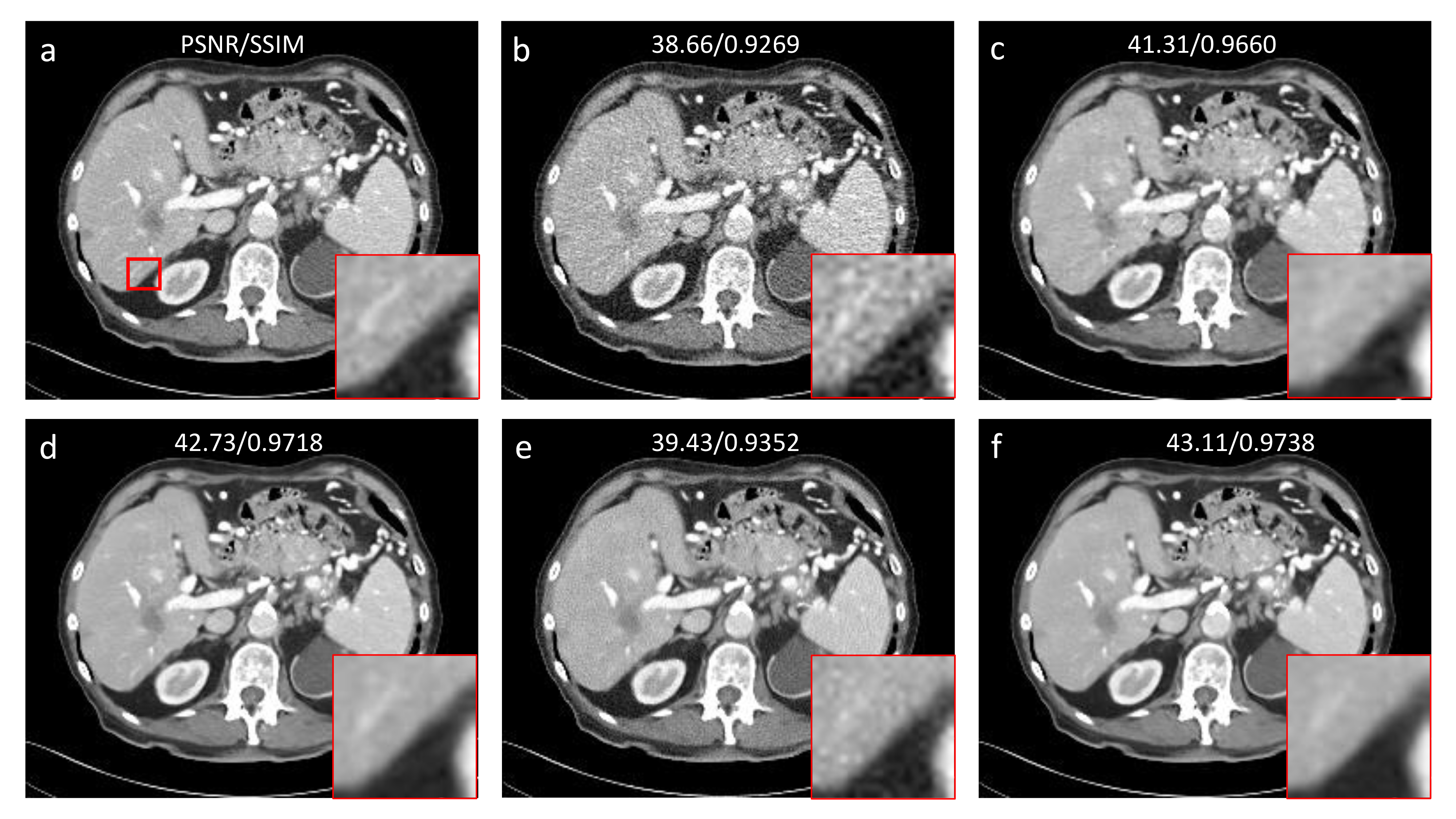
Figure 2: The results obtained using different methods. (a) NDCT, (b) LDCT, (c) U-Net, (d) DDPM, (e) DPM-Solver 15 NFE, and (f) DPM-Solver 50 NFE. The display window is consistently set to [-160, 240] HU.

3 Experiments and Results

To evaluate the performance of our proposed method for LDCT denoising, the 2016 NIH-AAPM-Mayo Clinic Low-Dose CT Grand Challenge dataset was chosen. The dataset has 2,378 paired NDCT and LDCT images with a thickness of 3mm from 10 patients. We selected 1,923 paired images from 8 patients as the training set, and 455 paired images from the remaining 2 patients as the test set. The image matrix was resampled to be 256x256. The total number of time steps $T$ was set to 1,000. The model was trained using the Adam optimizer kingma2014adam with a learning rate of $1\times 10^{-4}$. The training process converged well after $5\times 10^{5}$ iterations on a computing server equipped with Nvidia GTX 1080 Ti x4 GPUs. After the model was trained, we used DDPM, DPM-Solver 15 NFE and DPM-Solver 50 NFE to sample the test set respectively.

Fig. 2 shows the results obtained using different methods. It can be seen that U-Net ronneberger2015u failed to eliminate image noise completely. With DDPM, image noise was effectively removed while the structures were well kept. With only 15 NFE, the DPM-Solver could not denoise LDCT images well. Because of a too few number of sampling steps, residual noise and newly generated noise are evident in the resultant images sampled with DPM-Solver 15 NFE. Remarkably, after NFE was increased to 50, the DPM-solver delivered a competitive performance relative to that of DDPM. It can be seen that in the magnified region of interest (ROI), DPM-Solver 50 NFE well maintained the vasculature, which was blurred by U-Net. Quantitatively, DPM-Solver 50 NFE outperformed DDPM. Fig. 3 shows the absolute error maps of the abdominal results shown in Fig. 2 in reference to the NDCT image. It further demonstrates the efficient and effective sampling performance of the DPM-Solver, whose error map is the least noisy.

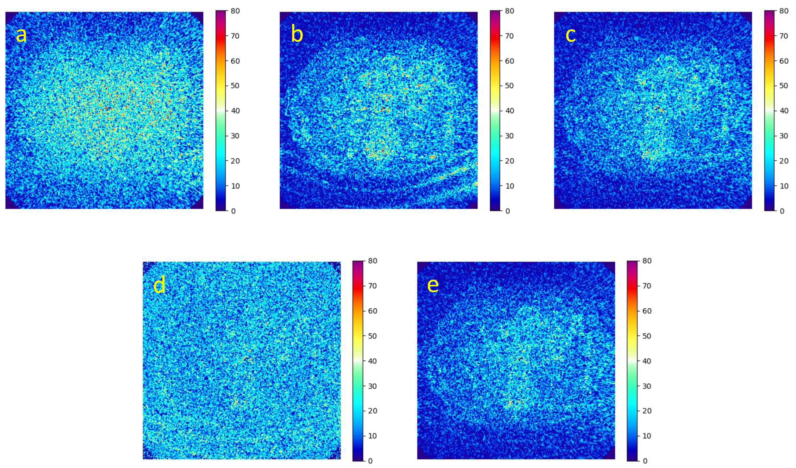
Figure 3: The absolute error maps of the results in reference to the NDCT image. (a) LDCT, (b) U-Net, (c) DDPM, (d) DPM-Solver 15 NFE, and (e) DPM-Solver 50 NFE. The display window is [0, 80] HU.

Table 1 shows the averaged quantitative evaluation of different methods over the whole test set. It can be seen that DDPM and DPM-Solver 50 NFE have the best quantitative scores. Especially, DPM-Solver 50 NFE quantitatively outperforms DDPM, which means that sampling with the DPM-Solver gives a superior noise suppression performance.

Table 1: Average quantitative results of different methods.

Method	PSNR	SSIM
LDCT	42.81	0.9667
U-Net	44.08	0.9823
DDPM	46.49	0.9873
DPM-Solver 15 NFE	40.41	0.9423
DPM-Solver 50 NFE	46.72	0.9880

Table 2 shows the averaged computational costs of different methods. Without any need for iterative sampling, U-Net has the highest processing efficiency. However, the denoising performance of U-Net is of limited value in clinical applications. DDPM requires a very high inference cost, which is hardly acceptable in practice. The DPM-Solver allows an excellent acceleration, while keeping or even improving the sampling quality. It can be seen that DPM-Solver 50 NFE achieves a 20$\times$ speedup compared to DDPM while maintaining denoising performance.

Table 2: Averaged inference costs of different methods

Method	Cost (second per image)
U-Net	0.08
DDPM	62.17
DPM-Solver 15 NFE	0.95
DPM-Solver 50 NFE	3.12

4 Conclusion

In this paper, we have adapted a novel conditional DDPM model for LDCT denoising. The denoising performance outperforms the traditional CNN-based method. Furthermore, to accelerate the sampling operation of DDPM, we have applied a fast ODE solver. It is shown that the ODE Solver has both a high denoising performance and a high sampling efficiency. Specifically, the ODE solver can achieve a 20$\times$ speedup without compromising the denoising performance. The superior performance of the ODE solver for DDPM sampling means a great potential for clinical applications.

References

- [1] Jonas Adler and Ozan Öktem. Learned primal-dual reconstruction. IEEE transactions on medical imaging, 37(6):1322–1332, 2018.
- [2] Kendall Atkinson, Weimin Han, and David E Stewart. Numerical solution of ordinary differential equations. John Wiley & Sons, 2011.
- [3] Jian-Feng Cai, Xun Jia, Hao Gao, Steve B Jiang, Zuowei Shen, and Hongkai Zhao. Cine cone beam ct reconstruction using low-rank matrix factorization: algorithm and a proof-of-principle study. IEEE transactions on medical imaging, 33(8):1581–1591, 2014.
- [4] Hu Chen, Yi Zhang, Yunjin Chen, Junfeng Zhang, Weihua Zhang, Huaiqiang Sun, Yang Lv, Peixi Liao, Jiliu Zhou, and Ge Wang. Learn: Learned experts’ assessment-based reconstruction network for sparse-data ct. IEEE transactions on medical imaging, 37(6):1333–1347, 2018.
- [5] Hu Chen, Yi Zhang, Mannudeep K Kalra, Feng Lin, Yang Chen, Peixi Liao, Jiliu Zhou, and Ge Wang. Low-dose ct with a residual encoder-decoder convolutional neural network. IEEE transactions on medical imaging, 36(12):2524–2535, 2017.
- [6] Hu Chen, Yi Zhang, Weihua Zhang, Peixi Liao, Ke Li, Jiliu Zhou, and Ge Wang. Low-dose ct via convolutional neural network. Biomedical optics express, 8(2):679–694, 2017.
- [7] Yang Chen, Dazhi Gao, Cong Nie, Limin Luo, Wufan Chen, Xindao Yin, and Yazhong Lin. Bayesian statistical reconstruction for low-dose x-ray computed tomography using an adaptive-weighting nonlocal prior. Computerized Medical Imaging and Graphics, 33(7):495–500, 2009.
- [8] Yang Chen, Xindao Yin, Luyao Shi, Huazhong Shu, Limin Luo, Jean-Louis Coatrieux, and Christine Toumoulin. Improving abdomen tumor low-dose CT images using a fast dictionary learning based processing. Physics in Medicine & Biology, 58(16):5803, 2013.
- [9] Zhiqiang Chen, Xin Jin, Liang Li, and Ge Wang. A limited-angle ct reconstruction method based on anisotropic tv minimization. Physics in Medicine & Biology, 58(7):2119–2141, 2013.
- [10] Jooyoung Choi, Sungwon Kim, Yonghyun Jeong, Youngjune Gwon, and Sungroh Yoon. Ilvr: Conditioning method for denoising diffusion probabilistic models. arXiv preprint arXiv:2108.02938, 2021.
- [11] Il Yong Chun, Zhengyu Huang, Hongki Lim, and Jeff Fessler. Momentum-net: Fast and convergent iterative neural network for inverse problems. IEEE transactions on pattern analysis and machine intelligence, 2020.
- [12] Florinel-Alin Croitoru, Vlad Hondru, Radu Tudor Ionescu, and Mubarak Shah. Diffusion models in vision: A survey. arXiv preprint arXiv:2209.04747, 2022.
- [13] Prafulla Dhariwal and Alexander Nichol. Diffusion models beat gans on image synthesis. Advances in Neural Information Processing Systems, 34:8780–8794, 2021.
- [14] John R Dormand and Peter J Prince. A family of embedded runge-kutta formulae. Journal of computational and applied mathematics, 6(1):19–26, 1980.
- [15] P Fumene Feruglio, Claudio Vinegoni, J Gros, A Sbarbati, and R Weissleder. Block matching 3d random noise filtering for absorption optical projection tomography. Physics in Medicine & Biology, 55(18):5401, 2010.
- [16] Hao Gao, Hengyong Yu, Stanley Osher, and Ge Wang. Multi-energy ct based on a prior rank, intensity and sparsity model (prism). Inverse problems, 27(11):115012, 2011.
- [17] Ian Goodfellow, Jean Pouget-Abadie, Mehdi Mirza, Bing Xu, David Warde-Farley, Sherjil Ozair, Aaron Courville, and Yoshua Bengio. Generative adversarial networks. Communications of the ACM, 63(11):139–144, 2020.
- [18] Harshit Gupta, Kyong Hwan Jin, Ha Q Nguyen, Michael T McCann, and Michael Unser. Cnn-based projected gradient descent for consistent ct image reconstruction. IEEE transactions on medical imaging, 37(6):1440–1453, 2018.
- [19] Yoseob Han and Jong Chul Ye. Framing u-net via deep convolutional framelets: Application to sparse-view ct. IEEE transactions on medical imaging, 37(6):1418–1429, 2018.
- [20] Jonathan Ho, Ajay Jain, and Pieter Abbeel. Denoising diffusion probabilistic models. Advances in Neural Information Processing Systems, 33:6840–6851, 2020.
- [21] Kyong Hwan Jin, Michael T McCann, Emmanuel Froustey, and Michael Unser. Deep convolutional neural network for inverse problems in imaging. IEEE Transactions on Image Processing, 26(9):4509–4522, 2017.
- [22] Dongwoo Kang, Piotr Slomka, Ryo Nakazato, Jonghye Woo, Daniel S Berman, C-C Jay Kuo, and Damini Dey. Image denoising of low-radiation dose coronary ct angiography by an adaptive block-matching 3d algorithm. In Medical Imaging 2013: Image Processing, volume 8669, pages 671–676. SPIE, 2013.
- [23] Eunhee Kang, Junhong Min, and Jong Chul Ye. A deep convolutional neural network using directional wavelets for low-dose x-ray ct reconstruction. Medical physics, 44(10):e360–e375, 2017.
- [24] Diederik Kingma, Tim Salimans, Ben Poole, and Jonathan Ho. Variational diffusion models. Advances in neural information processing systems, 34:21696–21707, 2021.
- [25] Diederik P Kingma and Jimmy Ba. Adam: A method for stochastic optimization. arXiv preprint arXiv:1412.6980, 2014.
- [26] Yann LeCun, Yoshua Bengio, and Geoffrey Hinton. Deep learning. nature, 521(7553):436–444, 2015.
- [27] Zhoubo Li, Lifeng Yu, Joshua D Trzasko, David S Lake, Daniel J Blezek, Joel G Fletcher, Cynthia H McCollough, and Armando Manduca. Adaptive nonlocal means filtering based on local noise level for ct denoising. Medical physics, 41(1):011908, 2014.
- [28] Cheng Lu, Yuhao Zhou, Fan Bao, Jianfei Chen, Chongxuan Li, and Jun Zhu. Dpm-solver: A fast ode solver for diffusion probabilistic model sampling in around 10 steps. arXiv preprint arXiv:2206.00927, 2022.
- [29] Andreas Lugmayr, Martin Danelljan, Andres Romero, Fisher Yu, Radu Timofte, and Luc Van Gool. Repaint: Inpainting using denoising diffusion probabilistic models. In Proceedings of the IEEE/CVF Conference on Computer Vision and Pattern Recognition, pages 11461–11471, 2022.
- [30] Chenlin Meng, Yang Song, Jiaming Song, Jiajun Wu, Jun-Yan Zhu, and Stefano Ermon. Sdedit: Image synthesis and editing with stochastic differential equations. arXiv preprint arXiv:2108.01073, 2021.
- [31] Alexander Quinn Nichol and Prafulla Dhariwal. Improved denoising diffusion probabilistic models. In International Conference on Machine Learning, pages 8162–8171. PMLR, 2021.
- [32] Shanzhou Niu, Yang Gao, Zhaoying Bian, Jing Huang, Wufan Chen, Gaohang Yu, Zhengrong Liang, and Jianhua Ma. Sparse-view x-ray ct reconstruction via total generalized variation regularization. Physics in Medicine & Biology, 59(12):2997–3017, 2014.
- [33] Eckhard Platen and Nicola Bruti-Liberati. Numerical solution of stochastic differential equations with jumps in finance, volume 64. Springer Science & Business Media, 2010.
- [34] Robin Rombach, Andreas Blattmann, Dominik Lorenz, Patrick Esser, and Björn Ommer. High-resolution image synthesis with latent diffusion models. In Proceedings of the IEEE/CVF Conference on Computer Vision and Pattern Recognition, pages 10684–10695, 2022.
- [35] Olaf Ronneberger, Philipp Fischer, and Thomas Brox. U-net: Convolutional networks for biomedical image segmentation. In International Conference on Medical image computing and computer-assisted intervention, pages 234–241. Springer, 2015.
- [36] Chitwan Saharia, William Chan, Huiwen Chang, Chris Lee, Jonathan Ho, Tim Salimans, David Fleet, and Mohammad Norouzi. Palette: Image-to-image diffusion models. In ACM SIGGRAPH 2022 Conference Proceedings, pages 1–10, 2022.
- [37] Chitwan Saharia, Jonathan Ho, William Chan, Tim Salimans, David J Fleet, and Mohammad Norouzi. Image super-resolution via iterative refinement. IEEE Transactions on Pattern Analysis and Machine Intelligence, 2022.
- [38] Hongming Shan, Atul Padole, Fatemeh Homayounieh, Uwe Kruger, Ruhani Doda Khera, Chayanin Nitiwarangkul, Mannudeep K Kalra, and Ge Wang. Competitive performance of a modularized deep neural network compared to commercial algorithms for low-dose ct image reconstruction. Nature Machine Intelligence, 1(6):269–276, 2019.
- [39] Jascha Sohl-Dickstein, Eric Weiss, Niru Maheswaranathan, and Surya Ganguli. Deep unsupervised learning using nonequilibrium thermodynamics. In International Conference on Machine Learning, pages 2256–2265. PMLR, 2015.
- [40] Yang Song and Stefano Ermon. Generative modeling by estimating gradients of the data distribution. Advances in Neural Information Processing Systems, 32, 2019.
- [41] Yang Song, Jascha Sohl-Dickstein, Diederik P Kingma, Abhishek Kumar, Stefano Ermon, and Ben Poole. Score-based generative modeling through stochastic differential equations. arXiv preprint arXiv:2011.13456, 2020.
- [42] Ge Wang. A perspective on deep imaging. IEEE access, 4:8914–8924, 2016.
- [43] Jelmer M Wolterink, Tim Leiner, Max A Viergever, and Ivana Išgum. Generative adversarial networks for noise reduction in low-dose ct. IEEE transactions on medical imaging, 36(12):2536–2545, 2017.
- [44] Dufan Wu, Kyungsang Kim, Georges El Fakhri, and Quanzheng Li. Iterative low-dose ct reconstruction with priors trained by artificial neural network. IEEE transactions on medical imaging, 36(12):2479–2486, 2017.
- [45] Jinxi Xiang, Yonggui Dong, and Yunjie Yang. Fista-net: Learning a fast iterative shrinkage thresholding network for inverse problems in imaging. IEEE Transactions on Medical Imaging, 40(5):1329–1339, 2021.
- [46] Qiong Xu, Hengyong Yu, Xuanqin Mou, Lei Zhang, Jiang Hsieh, and Ge Wang. Low-dose x-ray ct reconstruction via dictionary learning. IEEE transactions on medical imaging, 31(9):1682–1697, 2012.
- [47] Ling Yang, Zhilong Zhang, and Shenda Hong. Diffusion models: A comprehensive survey of methods and applications. arXiv preprint arXiv:2209.00796, 2022.
- [48] Qingsong Yang, Pingkun Yan, Yanbo Zhang, Hengyong Yu, Yongyi Shi, Xuanqin Mou, Mannudeep K Kalra, Yi Zhang, Ling Sun, and Ge Wang. Low-dose ct image denoising using a generative adversarial network with wasserstein distance and perceptual loss. IEEE transactions on medical imaging, 37(6):1348–1357, 2018.
- [49] Guoqiang Yu, Liang Li, Jianwei Gu, and Li Zhang. Total variation based iterative image reconstruction. In International Workshop on Computer Vision for Biomedical Image Applications, pages 526–534. Springer, 2005.
- [50] Yi Zhang, Yan Wang, Weihua Zhang, Feng Lin, Yifei Pu, and Jiliu Zhou. Statistical iterative reconstruction using adaptive fractional order regularization. Biomedical optics express, 7(3):1015–1029, 2016.
- [51] Yi Zhang, Weihua Zhang, Yinjie Lei, and Jiliu Zhou. Few-view image reconstruction with fractional-order total variation. JOSA A, 31(5):981–995, 2014.
- [52] Xuehang Zheng, Zening Lu, Saiprasad Ravishankar, Yong Long, and Jeffrey A Fessler. Low dose ct image reconstruction with learned sparsifying transform. In 2016 IEEE 12th Image, Video, and Multidimensional Signal Processing Workshop (IVMSP), pages 1–5. IEEE, 2016.