Modeling driver’s evasive behavior during safety-critical lane changes: Two-dimensional time-to-collision and deep reinforcement learning

Abstract

Lane changes are complex driving behaviors and frequently involve safety-critical situations. This study aims to develop a lane-change-related evasive behavior model, which can facilitate the development of safety-aware traffic simulations and predictive collision avoidance systems. Large-scale connected vehicle data from the Safety Pilot Model Deployment (SPMD) program were used for this study. A new surrogate safety measure, two-dimensional time-to-collision (2D-TTC), was proposed to identify the safety-critical situations during lane changes. The validity of 2D-TTC was confirmed by showing a high correlation between the detected conflict risks and the archived crashes. A deep deterministic policy gradient (DDPG) algorithm, which could learn the sequential decision-making process over continuous action spaces, was used to model the evasive behaviors in the identified safety-critical situations. The results showed the superiority of the proposed model in replicating both the longitudinal and lateral evasive behaviors.

1 Introduction

Lane changes are complicated driving behaviors that depend on the surrounding traffic dynamics, lane positions, and drivers’ motivations [Sun and Kondyli, 2010, Keyvan-Ekbatani et al., 2016, Ali et al., 2020, Zhang et al., 2021]. They might trigger conflicts in the interactions with the surrounding vehicles and activate the drivers’ evasive actions [Zheng et al., 2010, Zheng, 2014, Chen et al., 2021]. At the same time, lane changes could also be evasive actions in response to the potential risks [Petersen and Barrett, 2009, Xu et al., 2012]. It is critical to understand evasive behaviors during lane changes, given their complexity and significant safety impact. The accurate modeling of the vehicle’s motions under safety-critical conditions could contribute to the safety-aware traffic simulation [Gettman and Head, 2003, Markkula et al., 2012, Wang et al., 2018]. Besides, the advanced driving assistance system (ADAS) and the automated vehicle can incorporate useful information from the evasive behavior model to provide driver-specific control intervention and plan an evasive path consistent with human’s operating habits [Tseng et al., 2005, Happee et al., 2017, Soudbakhsh et al., 2011].

The accurate detection and extraction of safety-critical driving scenarios are fundamental for studying evasive behaviors. Compared to the traditional methods, which rely on historical crashes that often require a significant time to collect sufficient data [Scanlon et al., 2015], the approaches based on surrogate safety measures (SSMs) are more proactive. The SSMs could capture the more frequent "near-crash" situations and help understand the process of evasions or crashes [Li et al., 2020, 2021]. Many studies have used SSMs for risk identification and their correlation with the crash data has been affirmed [Xie et al., 2016, 2019, Yang et al., 2021b]. It is well accepted that the SSM-based approach can be used to identify and analyze safety-critical scenarios.

As an integral effort to improve traffic safety, driver’s evasive behavior models have received wide attention [Markkula et al., 2012, Dozza, 2013, Xiong et al., 2019, Scanlon et al., 2021]. Many kinematic-based approaches have been proposed to simulate the braking and/or steering behavior in near-crash situations [Markkula et al., 2016, Svärd et al., 2021]. Meanwhile, the reinforcement learning (RL) methods, which can capture and model the drivers’ actions sequentially, have been used in driving behavior modeling in recent years [Haydari and Yilmaz, 2020, Farazi et al., 2021]. The RL algorithms could be used to model both the upper-level decision making process [Li et al., 2022] and the lower-level vehicle motion control [Zhu et al., 2018]. The safety risk was usually considered as a component of the reward function [Zhu et al., 2020, Li et al., 2022]. Limited studies employed RL for evasive behavior modeling in pedestrian-related conflicts [Zuo et al., 2020, Nasernejad et al., 2021, Papini et al., 2021]. It is worth to further unlock the potential of RL approaches in driver’s evasive behavior modeling.

Video recording and driving simulator data were widely used to study evasive behaviors. These datasets either only cover limited driving scenarios or do not reflect the real driving experience. With the onboard sensors, the connected vehicles (CVs) could collect large-scale naturalistic motion data of the subject vehicle and its ambient traffic, which is beneficial for driver behavior modeling [Zhao et al., 2017, Guo et al., 2021, 2022]. The Safety Pilot Model Deployment (SPMD) program is a real-world CV test conducted by the U.S. Department of Transportation (USDOT) [Henclewood et al., 2014]. It provides rich high-resolution data for the identification of safety-critical situations and the development of evasive behavior models.

This study aims to develop a lane-change-related evasive behavior model using the CV data from the SPMD program. A novel SSM is proposed to capture the safety risk during lane changes. The deep deterministic policy gradient (DDPG) [Lillicrap et al., 2015] algorithm is used to imitate the drivers’ evasive behaviors. The remainder of this paper is organized as follows. In Section 2, a thorough literature review on the related research is carried out. The proposed two-dimensional time-to-collision (2D-TTC) and the DDPG model are introduced in Section 3. The detailed data processing procedure is illustrated in Section 4. In Section 5, the results and discussions are presented. At last, the conclusions of this study are summarized in Section 6.

2 Literature review

2.1 Surrogate safety measures

In the safety-related research, SSM is a proactive approach by capturing the more frequent near-crash situations, compared to the historical crash records. Time to collision (TTC) is one of the most widely used SSMs, which was introduced by Hayward [1972]. It is defined as the time required for two vehicles to collide if they continue in their present speed along the same path, and is calculated as

$$TTC=\left\{\begin{matrix}\frac{s_{0}-l}{v-v_{0}},&v>v_{0}\\ \infty,&otherwise\end{matrix}\right.$$ (1)

where $s_{0}$ is the space headway between the following and leading vehicles, $l$ is the length of the leading vehicle, $v_{0}$ and $v$ are the initial velocity of the leading and following vehicles, respectively. If the TTC value is less than a threshold, the car-following scenario is considered to be unsafe. Due to its simplicity and practicality, TTC has been widely used as a safety indicator in many studies [Lenard et al., 2018, Li et al., 2020, Deveaux et al., 2021, Li et al., 2021]. Based on TTC, Minderhoud and Bovy [2001] proposed time exposed TTC (TET) and time integrated TTC (TIT). They were able to include the duration of dangerous driving scenarios into risk measurement and were also applied in several studies [Jamson et al., 2013, Li et al., 2017, Yang et al., 2021a].

However, there are two major shortcomings of the conventional TCC: i) the scenario is regarded as safe when the speed of the following vehicle is less than or equal to that of the leading vehicle, even though the relative distance could be very small [Kuang et al., 2015]; and ii) the vehicle pair is assumed in the same lane and only the longitudinal movements are calculated [Xing et al., 2019]. To address these limitations, some researchers included the speed changes of vehicles into TTC. Ozbay et al. [2008] modified TTC by considering all the potential longitudinal conflicts related to acceleration or deceleration. Xie et al. [2019] imposed a hypothetical disturbance to the leading vehicle and derived the TTC with disturbance (TTCD). It has been proved that TTCD was capable to identify high-risk locations and assess safety performance with real-world data [Yang et al., 2021b].

Some other studies concentrated on expanding the TTC to the two-dimensional road plane and proposed the trajectory-based SSMs. Hou et al. [2014] proposed algorithms for computing TTC by solving the two-dimensional distance equations and validated them with simulation models. Ward et al. [2015] generalized TTC to the two-dimensional movement case and derived a method for predicting conflicting trajectories based on the relative movement between two vehicles. Venthuruthiyil and Chunchu [2022] proposed anticipated collision time (ACT) for the two-dimensional trajectory-based proactive safety assessment. However, these SSMs relied on the recorded complete trajectories and could not estimate the potential risks instantly. In this study, the CVs are probe vehicles, moving around and collecting data only from themselves and surrounding vehicles. It is expensive to reconstruct the complete trajectories of all vehicles from the CV data. Furthermore, to facilitate collision avoidance systems, safety risks should be captured in real time instead of offline. A new TTC that is customized for CV data and capable for capturing the conflict instantaneously is needed.

2.2 Evasive behavior

As one of the bases to improve traffic safety, it is crucial to understand and model the evasive behaviors of drivers accurately under safety-critical conditions [Markkula et al., 2012]. Many researchers have been focusing on evasive behavior modeling, and the findings can be categorized into three groups according to the maneuvers, namely evading by braking (longitudinal acceleration) alone, steering (lateral acceleration) alone, and the interplay of braking and steering.

Both the naturalistic and simulator-based studies indicate that braking is the most common avoidance response [McGehee et al., 1999, Najm et al., 2013]. Thus, the braking behavior in pre-crash situations has been a research hot spot [Markkula et al., 2016, Svärd et al., 2017, Xue et al., 2018, Svärd et al., 2021]. The steering behavior is less common in evasion, as it might involve more decision factors, such as the surrounding traffic situations. It is expected to help avoid the collision that cannot be avoided by braking only and has drawn some research attention [Shibata et al., 2014, Yuan et al., 2019, Zheng et al., 2020].

The combination of braking and steering evasive behaviors has the potential to further reduce the probability of collisions [Horiuchi et al., 2001, Schmidt et al., 2006]. However, there are limited studies on the combined evasive behavior due to its complexity. Some studies focused on predicting the driver’s choice of evasive behavior (braking or steering) using classification methods [Venkatraman et al., 2016, Sarkar et al., 2021]. Further studies focused on modeling the driver’s braking and steering actions. Sugimoto and Sauer [2005] assumed an evasive behavior model including braking and steering, and used it to evaluate the effectiveness of ADAS. Jurecki and Stańczyk [2009] designed a model for collision avoidance at intersections based on the results of track tests. Both the barking and steering behaviors could be reconstructed successfully in pre-crash situations. Markkula [2014] proposed a framework to model the drivers’ steering and pedal behaviors as a series of individual control adjustments. Schnelle et al. [2018] presented an integrated feedback and feedforward driver model, which could represent the driver’s control actions in safety-critical scenarios. Zhou and Zhong [2020] developed statistical models from near-crash trajectories and drew evasive behaviors from the joint probability distributions.

In most studies, the evasive behavior models were built based on the data from driving simulators or track tests, which may not reflect real-world driving situations. A limited number of studies adopted the crash and near-crash records for model development [Markkula et al., 2016, Zhou and Zhong, 2020, Svärd et al., 2021, Sarkar et al., 2021], while the historical crashes data often requires a significant time for collection. Besides, the kinematic-model-based approaches were widely used in these studies. The models with assumed constraints might be not flexible enough to simulate evasive behavior, since the extreme driving behavior is likely to be taken in safety-critical situations. Meanwhile, the data-driven methods have been widely applied in driving behavior modeling due to their flexibility and outperformed accuracy [Huang et al., 2018, Lee et al., 2019, Xing et al., 2020, Ma and Qu, 2020]. It is worth to develop a proactive SSM-based approach for risk detection and build an evasive behavior model with data-driven approaches.

2.3 Reinforcement learning in driving behavior modeling

RL is a machine learning approach aiming to let an intelligent agent interact with an environment and make decisions. The agent is trained to learn the optimal policy that maximizes the reward function. The basic RL is modeled as a Markov decision process (MDP). At each time step $t$, the RL agent is at a state $S_{t}$. It chooses an action $A_{t}$ according to the policy $\pi(A_{t}|S_{t})$, which is subsequently sent to the environment. Then, the agent moves to a new state $S_{t+1}$ and receives a reward $R_{t}$. The MDP continues until the system reaches a terminal state and it will restart. The agent aims to maximize the discounted accumulated reward function $\sum R_{t}=\sum_{k=0}^{\infty}\gamma^{k}R_{t+k}$, with the discount factor $\gamma\in(0,1]$ [Li, 2017]. As the RL algorithm improves its policies by interacting with the environment, it is suitable for problems whose solutions can be optimized by trial-and-error. It is also appropriate for the problems that emphasize task completion and delayed reward over the periodical success at intermediate steps. Because of these features, RL was widely applied in transportation studies and provided promising results [Abdulhai and Kattan, 2003, Ozan et al., 2015, Aslani et al., 2017, Essa and Sayed, 2020].

Deep reinforcement learning (DRL) is the combination of RL and deep learning (DL). The policy and other learned functions are often represented as neural networks. As DL is incorporated into the RL solution, the agent is able to make decisions from complex and high-dimensional raw input data with less manual engineering of the state space. Due to the ability to generate high-quality solutions and generality in solving varying problems, DRL has been widely used in driving behavior modeling aiming at the application of autonomous vehicles [Haydari and Yilmaz, 2020, Farazi et al., 2021]. It could be used for both the upper-level driving behavior decision making [Dong et al., 2021, Wang et al., 2021, Li et al., 2022] and the lower-level vehicle motion control [Zhu et al., 2018, Ye et al., 2019, Zhu et al., 2020, Tian et al., 2021].

As for the application of RL in traffic safety, the safety factors were often included and modeled as a component of the reward function in some of the aforementioned studies [Ye et al., 2019, Zhu et al., 2020, Dong et al., 2021]. Li et al. [2022] assessed the risk of lane change decision and used a deep Q-network (DQN), a widely used model of DRL, to find the strategy with the minimum expected risk. The model outperformed the baseline models without risk assessment in terms of average traveled distance. There was also limited research using DRL to model the drivers’ evasive behaviors in critical situations. Chae et al. [2017] developed an autonomous braking system with DQN, which decided whether to apply the brake when confronting the risk of collision. Zuo et al. [2020] used RL to determine the optimal timing to cross the intersection with the consideration of pedestrian safety. Papini et al. [2021] studied the scenario that a pedestrian suddenly crossing the road and employed DQN to choose an appropriate speed, which enabled the autonomous vehicle to perform an emergency braking maneuver successfully. Besides, the RL approaches were used to model the behaviors in pedestrian-cyclist conflicts [Nasernejad et al., 2021, Alsaleh and Sayed, 2021].

Most of the existing studies are developed based on traffic simulations, as it is a noise-free interactive environment for the RL agent. Only a small portion of previously mentioned research used human driving data, either the driving simulator data [Tian et al., 2021] or the video-based real-world data [Zhu et al., 2020, 2018, Nasernejad et al., 2021, Alsaleh and Sayed, 2021, Shi et al., 2021]. Although the models achieved good performance in the simulation environment, they might not be able to reflect real situations. Additionally, the video-based data are collected with a limited range of roads or intersections, which may not cover various traffic scenarios under different conditions. It is critical to develop the evasive behavior model using large-scale real-world data.

3 Methodology

3.1 2-dimensional time-to-collision

To address the limitations of TTC discussed in the literature review, we extended the TTC to a two-dimensional plane and proposed a new TTC called 2D-TTC. The proposed approach relaxes the constraint of the vehicle pair’s positions and motions. It is also suitable for real-time risk measurement based on onboard sensors of CVs.

Similar to TTC, the leading and following vehicles are assumed to maintain their current speeds and directions. The trajectory of each vehicle will be estimated, and the collision is detected based on their estimated positions. Both the longitudinal and lateral risks could be captured by 2D-TTC. Additionally, it is intuitive as it is based on the well-known and widely used concept of TTC.

A general two-dimensional traffic scenario at the initial time $t_{0}$ is illustrated in Fig. 1. $s_{0}$ is the spacing headway between the two vehicles, $v_{0}$ and $v$ are the speed of the leading and following vehicles, respectively. It is assumed that the two vehicles have the same length $l$ and width $w$. The longitudinal and lateral components of $s_{0}$, $v_{0}$, and $v$ are denoted as $s_{0lon}$, $v_{0lon}$, $v_{lon}$, and $s_{0lat}$, $v_{0lat}$, $v_{lat}$, respectively.

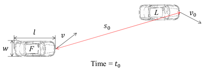
Figure 1: A 2-D traffic scenario

Depending on the relative positions of the two vehicles, there are two possible collision outcomes: i) longitudinal collision - the front end of the following vehicle hit the rear end of the leading vehicle; and ii) lateral collision - one side of the following vehicle hit the other side of the leading vehicle. These two types of collision will be analyzed and computed separately.

• Longitudinal collision and longitudinal time to collision

The longitudinal time-to-collision ($TTC_{lon}$) is defined as the time required for the front end of the following vehicle to reach the same longitudinal position as the rear end of the leading vehicle. If $s_{0lon}>l$ and $v_{lon}>v_{0lon}$, $TTC_{lon}$ is calculated as

$$TTC_{lon}=\frac{s_{0lon}-l}{v_{lon}-v_{0lon}}$$ (2)

When the two vehicles arrive at the assumed positions at time $t_{0}+TTC_{lon}$, there are three possible cases of their relative positions, as shown in Fig. 2.

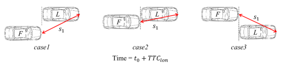
Figure 2: Longitudinal collision scenarios

The occurrence of collision depends on the remaining lateral distance $s_{1lat}$, which is given by Eq. (3):

$$s_{1lat}=s_{0lat}-(v_{lat}-v_{0lat})\cdot TTC_{lon}=s_{0lat}-(v_{lat}-v_{0lat})\cdot\frac{s_{0lon}-l}{v_{lon}-v_{0lon}}$$ (3)

If $s_{1lat}>w$ (case1 or case3), there is no lateral overlap of the two vehicles, and thus no collision occurs. If $s_{1lat}\leq w$ (case2), a rear-end collision would happen. By summarizing the computation and collision conditions, $TTC_{lon}$ is calculated as

$$TTC_{lon}=\left\{\begin{matrix}\frac{s_{0lon}-l}{v_{lon}-v_{0lon}},&s_{0lon}>l\wedge v_{lon}>v_{0lon}\wedge s_{0lat}-(v_{lat}-v_{0lat})\cdot\frac{s_{0lon}-l}{v_{lon}-v_{0lon}}<w\\ \infty,&otherwise\end{matrix}\right.$$ (4)

• Lateral collision and lateral time-to-collision

The lateral time-to-collision ($TTC_{lat}$) is defined as the time required for the left (right) side of the following vehicle to reach the same lateral position as the right (left) side of the leading vehicle. If $s_{0lat}>w$ and $v_{lat}>v_{0lat}$, $TTC_{lat}$ is calculated as

$$TTC_{lat}=\frac{s_{0lat}-w}{v_{lat}-v_{0lat}}$$ (5)

When the two vehicles arrive at the assumed positions at time $t_{0}+TTC_{lat}$, there are three possible cases of their relative positions, as shown in Fig. 3.

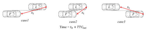
Figure 3: Sideswipe collision scenario

The occurrence of collision depends on the remaining longitudinal distance $s_{1lon}$, which is given by Eq. 6.

$$s_{1lon}=s_{0lon}-(v_{lon}-v_{0lon})\cdot TTC_{lat}=s_{0lon}-(v_{lon}-v_{0lon})\cdot\frac{s_{0lat}-w}{v_{lat}-v_{0lat}}$$ (6)

If $s_{1lon}>l$ (case1 or case3), there is no longitudinal overlap of the two vehicles, and thus no collision occurs. If $s_{1lon}\leq l$ (case2), a sideswipe collision would happen. By summarizing the computation and collision conditions, $TTC_{lat}$ is calculated as

$$TTC_{lat}=\left\{\begin{matrix}\frac{s_{0lat}-w}{v_{lat}-v_{0lat}},&s_{0lat}>w\wedge v_{lat}>v_{0lat}\wedge s_{0lon}-(v_{lon}-v_{0lon})\cdot\frac{s_{0lat}-w}{v_{lat}-v_{0lat}}<l\\ \infty,&otherwise\end{matrix}\right.$$ (7)

By combining the computations of $TTC_{lon}$ and $TTC_{lat}$, the unified function of $TTC_{2D}$ is expressed as

$$TTC_{2D}=min(TTC_{lon},TTC_{lat})$$ (8)

The type of conflict can also be classified with 2D-TTC. Specifically, if $TTC_{lon}\leq TTC_{lat}$, there would be a potential longitudinal (rear-end) crash; if $TTC_{lat}<TTC_{lon}$, there would be a potential lateral (sideswipe) crash. In the implementation of 2D-TTC, both the longitudinal and lateral conflicts should be considered jointly. Because the types of captured conflicts are interchangeable with the disturbances. Similar to TTC, an appropriate threshold is needed to differentiate the risky and safe scenarios. The vehicle pair with 2D-TTC lower than the threshold is involved in conflicts.

Clearly, the 2D-TTC is not only related to the relative distance and speed of the two vehicles but also their initial positions and directions. In this case, the vehicle pair not in the same path (i.e. a cut-in vehicle from the adjacent lane) could still yield risk rather than be regarded as safe by the conventional TTC. Besides, the 2D-TTC is computed based on the predicted trajectories, which overcomes the shortcomings of trajectory-based SSMs and is capable for real-time risk estimation.

3.2 Deep deterministic policy gradient

DDPG [Lillicrap et al., 2015] is a model-free off-policy reinforcement learning algorithm, whose deep function approximators could capture complex non-linear relationships. It uses the actor-critic approach from DPG (deterministic policy gradient) [Silver et al., 2014] to deal with the policy in the continuous action space. Besides, it employs the experience replay and soft-updating target networks from DQN [Mnih et al., 2015], in order to reduce the correlation among samples and improve the learning efficiency and stability. The architecture of DDPG is illustrated in Fig. 4, where the red arrows represent the experience generation process, and the blue arrows represent the training procedure.

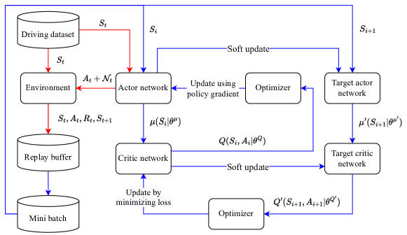
Figure 4: The architecture of DDPG, including the experience generation (red arrows) and training (blue arrows) processes

The DDPG model consists of four neural networks, namely the actor ($\mu$), target actor ($\mu^{\prime}$), critic ($Q$), and target critic ($Q^{\prime}$) network. The actor networks ($\mu$ and $\mu^{\prime}$) interact with the environment according to the given state and their weights. Then, the critic networks ($Q$ and $Q^{\prime}$) evaluate the action and output $Q$-values, which would be used for the model update. The target networks ($\mu^{\prime}$ and $Q^{\prime}$) are the lagged version of the actual agent networks ($\mu$ and $Q$), which are used to improve the algorithm’s stability.

In this study, the observed state $S_{t}=(d_{lon}(t),v_{lon}(t),\Delta v_{lon}(t),d_{lat}(t),v_{lat}(t),\Delta v_{lat}(t))$ at the time step $t$ is sampled from the naturalistic driving dataset, where $d_{lon}(t)$ and $d_{lat}(t)$ are the longitudinal and lateral distances to the leading vehicle, $v_{lon}(t)$ and $v_{lat}(t)$ are the CV’s longitudinal and lateral speed, and $\Delta v_{lon}(t)$ and $\Delta v_{lat}(t)$ are the longitudinal and lateral relative speed, respectively. The action generated by the agent is $A_{t}=(\hat{a}_{lon}(t),\hat{a}_{lat}(t))$, which is composed of the longitudinal acceleration $\hat{a}_{lon}(t)$ and the lateral acceleration $\hat{a}_{lat}(t)$. Then, a noise process ($\mathcal{N}$) is employed to explore the state and action spaces beyond the dataset. The Ornstein-Uhlenbeck process ($\theta=0.15$ and $\sigma=0.2$) [Uhlenbeck and Ornstein, 1930] is used to generate the temporally correlated noise for a better exploration of physical environments with momentum. The sampled noise will be added to the action and used in the state update. In order to let the agent interact with the environment, a kinematic model is constructed for state updating, which is presented as

$$\hat{v}_{lon}(t+1)=v_{lon}(t)+\hat{a}_{lon}(t)\Delta t$$ (9)

$$\Delta\hat{v}_{lon}(t+1)=\Delta v_{lon}(t)-\hat{a}_{lon}(t)\Delta t$$

$$\hat{d}_{lon}(t+1)=d_{lon}(t)+(v_{lon}(t)+\Delta v_{lon}(t))\Delta t-\frac{v_{lon}(t)+\hat{v}_{lon}(t+1)}{2}\Delta t$$

$$\hat{v}_{lat}(t+1)=v_{lat}(t)+\hat{a}_{lat}(t)\Delta t$$

$$\Delta\hat{v}_{lat}(t+1)=\Delta v_{lat}(t)-\hat{a}_{lat}(t)\Delta t$$

$$\hat{d}_{lat}(t+1)=d_{lat}(t)+(v_{lat}(t)+\Delta v_{lat}(t))\Delta t-\frac{v_{lat}(t)+\hat{v}_{lat}(t+1)}{2}\Delta t$$

where $\hat{v}_{lon}(t+1),\Delta\hat{v}_{lon}(t+1),\hat{d}_{lon}(t+1),\hat{v}_{lat}(t+1),\Delta\hat{v}_{lat}(t+1)$ and $\hat{d}_{lat}(t+1)$ are the simulated longitudinal speed, longitudinal relative speed, longitudinal distance, lateral speed, lateral relative speed and lateral distance at time step $t+1$, respectively. $\Delta t$ is the update time interval, which is 0.1s in this study. Three different reward functions, namely the distance reward ($R_{d}$), the speed reward ($R_{v}$), and the speed difference reward ($R_{\Delta v}$), are given by Eq. (10), Eq. (11), and Eq. (12), respectively. A small $\epsilon$ value ($\epsilon=1\times 10^{-7}$) is added to avoid dividing by zero. The reward functions are designed to let the network imitate human drivers’ behaviors and explore the underlying strategies by minimizing the difference in vehicle motions. At last, a set of experience ($S_{t},A_{t},R_{t},S_{t+1}$) will be stored in the replay buffer.

$$R_{d}=-(\frac{|\hat{d}_{lon}(t+1)-d_{lon}(t+1)|}{|d_{lon}(t+1)|+\epsilon})-(\frac{|\hat{d}_{lat}(t+1)-d_{lat}(t+1)|}{|d_{lat}(t+1)|+\epsilon})$$ (10)

$$R_{v}=-(\frac{|\hat{v}_{lon}(t+1)-v_{lon}(t+1)|}{|v_{lon}(t+1)|+\epsilon})-(\frac{|\hat{v}_{lat}(t+1)-v_{lat}(t+1)|}{|v_{lat}(t+1)|+\epsilon})$$ (11)

$$R_{\Delta v}=-(\frac{|\Delta\hat{v}_{lon}(t+1)-\Delta v_{lon}(t+1)|}{|\Delta v_{lon}(t+1)|+\epsilon})-(\frac{|\Delta\hat{v}_{lat}(t+1)-\Delta v_{lat}(t+1)|}{|\Delta v_{lat}(t+1)|+\epsilon})$$ (12)

At the beginning of the model training process, a random mini-batch of $N$ transitions ($S_{i},A_{i},R_{i},S_{i+1}$) are sampled from the replay buffer. The critic network evaluates the action and outputs the scalar $Q$-value $Q(S_{i},A_{i}|\theta^{Q})$ according to its weights $\theta^{Q}$. Similarly, the target actor network chooses the action $A_{i+1}=\mu^{\prime}(S_{i+1}|\theta^{\mu^{\prime}})$ based on the next-step state $S_{i+1}$, and the target critic network evaluates it with $Q^{\prime}(S_{i+1},A_{i+1}|\theta^{Q^{\prime}})$. The effect of the current action in the next step is taken into account in this step. Then, the critic network is updated by minimizing the loss $L=\frac{1}{N}\Sigma_{i}(y_{i}-Q(S_{i},A_{i}|\theta^{Q}))^{2}$, where $y_{i}=R_{i}+\gamma Q^{\prime}(S_{i+1},A_{i+1}|\theta^{Q^{\prime}})$. The actor network is updated using the sampled policy gradient $\nabla_{\theta\mu}J\approx\frac{1}{N}\sum_{i}\nabla_{A}Q(S,A|\theta^{Q})|_{S=S_{i},A=\mu(S_{i})}\nabla_{\theta\mu}\mu(S|\theta^{\mu})|_{S_{i}}$. In the end, the target actor and critic networks are soft updated with $\theta^{Q^{\prime}}\leftarrow\tau\theta^{Q}+(1-\tau)\theta^{Q^{\prime}}$ and $\theta^{\mu^{\prime}}\leftarrow\tau\theta^{\mu}+(1-\tau)\theta^{\mu^{\prime}}$, respectively. The detailed DDPG algorithm is presented in Algorithm 1.

Algorithm 1 DDPG algorithm (based on Lillicrap et al. [2015])

Randomly initialize critic network $Q(S,A|\theta^{Q})$ and actor $\mu(S|\theta^{\mu})$ with weights $\theta^{Q}$ and $\theta^{\mu}$
Initialize target network $Q^{\prime}$ and $\mu^{\prime}$ with weights $\theta^{Q^{\prime}}\leftarrow\theta^{Q}$, $\theta^{\mu^{\prime}}\leftarrow\theta^{\mu}$
Initialize replay buffer $B$

for episode=1, M do

     Initialize a random process $\mathcal{N}$ for action exploration

     Receive initial observation state $S_{1}$

     for t=1, T do

         Select action $A_{t}=\mu(S_{t}|\theta^{\mu})+\mathcal{N}_{t}$ according to the current policy and exploration noise

         Execute action $A_{t}$ and observe reward $R_{t}$ and observe new state $S_{t+1}$

         Store transition $(S_{t},A_{t},R_{t},S_{t+1})$ in $B$

         Sample a random minibatch of $N$ transitions $(S_{i},A_{i},R_{i},S_{i+1})$ from $B$

         Set $y_{i}=R_{i}+\gamma Q^{\prime}(S_{i+1},\mu^{\prime}(S_{i+1}|\theta^{\mu^{\prime}})|\theta^{Q^{\prime}})$

         Update critic by minimizing the loss: $L=\frac{1}{N}\Sigma_{i}(y_{i}-Q(S_{i},A_{i}|\theta^{Q}))^{2}$

         Update the actor policy using the sampled policy gradient:

$\nabla_{\theta\mu}J\approx\frac{1}{N}\sum_{i}\nabla_{A}Q(S,A|\theta^{Q})|_{S=S_{i},A=\mu(S_{i})}\nabla_{\theta\mu}\mu(S|\theta^{\mu})|_{S_{i}}$

         Update the target networks:

$\theta^{Q^{\prime}}\leftarrow\tau\theta^{Q}+(1-\tau)\theta^{Q^{\prime}}$ $\theta^{\mu^{\prime}}\leftarrow\tau\theta^{\mu}+(1-\tau)\theta^{\mu^{\prime}}$

     end for

end for

4 Data preparation

SPMD is the world’s largest CV test program, which aims to demonstrate CV technologies in the real-world environment [Huang et al., 2017]. 2,842 equipped vehicles participated in the program for over 2 years in Ann Arbor, Michigan [Bezzina and Sayer, 2014]. The two-month sample data (October 2012 and April 2013) are now available to the public on the ITS Data Hub (https://www.its.dot.gov/data/). The SPMD environment includes eight datasets, namely Data Acquisition System 1 (DAS1), Data Acquisition System 2 (DAS2), Basic Safety Message (BSM), Roadside Equipment, Network, Weather, Schedule, and Road Work Activity [Hamilton and Allen, 2015].

The DAS1 dataset, collected by the University of Michigan Transportation Research Institute (UMTRI) in April 2013, was used in this study. A total of 7,960 trips recorded by 98 sedans equipped with the DAS1 and the MobilEye sensor [Harding et al., 2014] were investigated. Within the DAS1 dataset, the DataLane file records the CVs’ lateral positions relative to lane boundaries (LaneDistanceLeft and LaneDistanceRight) and the estimated lane marking measurement quality (LaneQualityLeft and LaneQualityRight). The DataFrontTargets file provides relative positions (Range and Transversal) and relative speed (RangeRate) of the leading vehicles. The DataWsu file contains the geographical positions (LatitudeWsu and LongitudeWsu) and kinematics (GpsSpeedWsu and AxWsu) of CVs. The detailed description of the fields is reported in Table 1. All the data elements were collected at a frequency of 10 Hz. The DataLane and DataFrontTargets files were recorded by the MobilEye sensor, and the DataWsu file was collected by the GPS unit and controller area network (CAN) bus via the wireless safety unit (WSU). Python programming language [Van Rossum and Drake, 2009] with Apache Spark bigdata analytic engine [Zaharia et al., 2016] was used for big data manipulation.

Table 1: Field description of CV data

Origin File	Field Name	Description
Common	Device	A unique, numeric ID assigned to each DAS
	Trip	Count of ignition cycles—each ignition cycle commences when the ignition is in the on position and ends when it is in the off position
	Time	Time in centiseconds since DAS started, which (generally) starts when the ignition is in the on position ($centisecond$)
DataLane	LaneDistanceLeft ($d_{l}$)	Distance between the center line of the vehicle and the left boundary of the travel lane ($m$)
	LaneDistanceRight ($d_{r}$)	Distance between the center line of the vehicle and the right boundary of the travel lane ($m$)
	LaneQualityLeft	Quality of the estimated boundary measure of the travel lane’s left boundary (ranging from 0 "very bad" to 3 "very good")
	LaneQualityRight	Quality of the estimated boundary measure of the travel lane’s left boundary (ranging from 0 "very bad" to 3 "very good")
DataFrontTargets	ObstacleId	ID of new obstacle, as assigned by the Mobileye sensor, and its value will be the last used free ID
	TargetType	Classification of an identified obstacle/target (0: car; 1: truck; 2: motorcycle; 3: pedestrian; 4: bicycle)
	Range ($d_{lon}$)	Longitudinal position of an object, typically the closest object, relative to a reference point on the host vehicle, according to the Mobileye sensor ($m$)
	RangeRate ($\Delta v_{lon}$)	Longitudinal velocity of an object, typically the closest object, relative to the host vehicle, according to the Mobileye sensor ($m/s$)
	Transversal ($d_{lat}$)	The lateral position of the obstacle, as determined by the Mobileye sensor ($m$)
DataWsu	GpsValidWsu	Communicates whether a GPS data point is valid (1) or not (0)
	LatitudeWsu	Latitude from WSU receiver ($deg$)
	LongitudeWsu	Longitude from WSU receiver ($deg$)
	GpsSpeedWsu ($v_{lon}$)	Speed from WSU GPS receiver ($m/s$)
	ValidCanWsu	Vehicle CAN Bus message to WSU is valid (1) or not(0)
	AxWsu	Longitudinal acceleration from vehicle CAN Bus vis WSU ($m/s^{2}$)

To begin with, the invalid records were filtered out from the dataset. The criterion "LaneQualityLeft > 0 and LaneQualityRight > 0" was used to remove records with poor distance measurement quality. The data points with valid GPS and Can Bus messages were extracted with the criterion "GpsValidWsu = 1 and ValidCanWsu = 1". As the MobilEye sensor can track and identify different types of front objects, the criterion "TargetType = 0" was employed to ensure the leading vehicles are cars. After the cleaning process, all three datasets were merged based on the common fieldsDevice, Trip, and Time.

Then, some records were filtered out based on their values. According to the technical report [Kelly Blue Book, 2013], the fastest sedan can travel at a speed of 200mph (90m/s), and the maximum acceleration is around $\rm 7m/s^{2}$ in 2013. The record with GpsSpeedWsu value higher than 90m/s, or AxWsu value greater than $\rm 7m/s^{2}$ was removed as outliers. The MobilEye sensor could cover three or more lanes and track multiple targets, including the parking and reversing vehicles on the roadside, as well as the vehicles in the opposite direction. So the speed of the leading vehicle, calculated by GpsSpeedWsu + Rangerate, needs to be examined. Considering that the reversing vehicle may have potential conflict with the ego vehicle, the criterion "GpsSpeedWsu + Rangerate > -1m/s" was employed to filter out the records describing vehicles in the opposite direction. Besides, the free-flow scenarios were eliminated with the rule "Range < 100m". The criterion "-7m < Transversal < 7m" was applied to ensure that the leading vehicle is in the same or adjacent lane of the subject vehicle.

Next, the data would be filtered to reduce the influence of noise. The measurement quality of lane distance data ($LaneDistanceLeft$ and $LaneDistanceRight$) is not satisfactory, and the estimated quality ($LaneQualityLeft$ and $LaneQualityRight$) is usually less than 3. Because the lane markings might be uncontinuous and unclear, and they could be shaded by other vehicles. A Gaussian filter was adopted to process the lane distance data for noise reduction. The raw and processed data are shown in Fig 5. The computation of lateral speed is based on the lane distance data, which is given by Eq. 14. It is obvious that the Gaussian filter can effectively reduce the fluctuation of lateral speed without changing the lateral distance significantly.

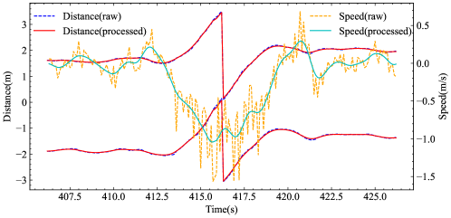
Figure 5: The raw and processed lateral distance and speed data

At last, the driving scenarios related to lane change were extracted. From the impact of the lane change on the traffic flow perspective, it lasts for about 25s on average [Ma and Ahn, 2008, Wang and Coifman, 2008]. Zheng et al. [2013] pointed out that the average duration for the anticipation and relaxation processes of lane change is 8-14s and 10-15s, respectively. To cover the complete process of lane change maneuver, the lane change events were selected 15s before and 15s after the time step of the vehicle crossing the lane boundary. Based on the findings in Guo et al. [2022], 2,199 left and 1,663 right lane change samples were detected from the SPMD dataset, which will be used for 2D-TTC computation and evasive behavior model development. The detailed data preparation procedure is illustrated in Fig. 6.

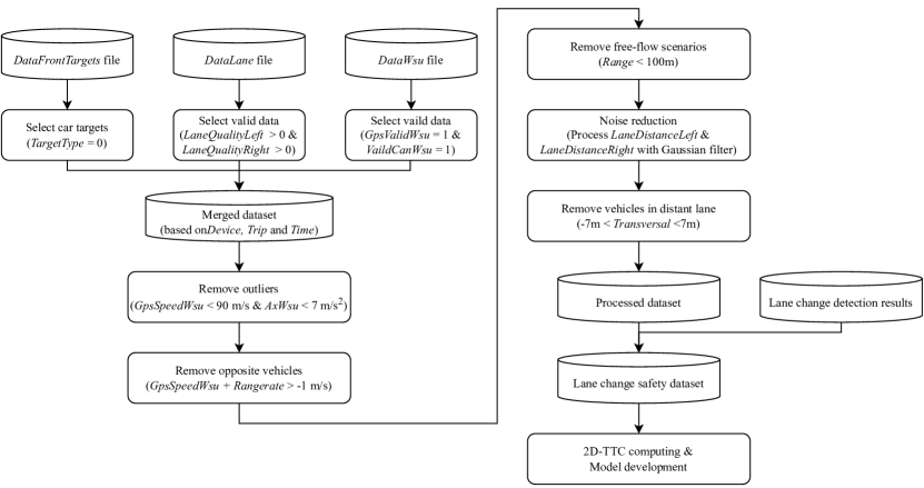
Figure 6: Data preparation procedure

In the processed lane change safety dataset, the longitudinal speed of the ego vehicle $v_{lon}=GpsSpeedWsu$ and the relative lateral distance $s_{0lat}=Transversal$ can be exported. Other variables in the 2D-TTC equations are calculated as

$$s_{0lon}=d_{lon}+l$$ (13)

$$v_{lat}=\frac{(d_{l}(t)-d_{l}(t-1))+(d_{r}(t)-d_{r}(t-1))}{2\times\Delta t}$$ (14)

$$v_{0lon}=v_{lon}+\Delta v_{lon}$$ (15)

$$v_{0lat}=v_{lat}+\frac{s_{0lat}(t)-s_{0lat}(t-1)}{\Delta t}$$ (16)

where $\Delta t$ is the time interval between two continuous records, which is 0.1s in the dataset. The length and width of leading cars are assumed to be 4.8m and 1.6m, based on the average car size.

5 Results and discussion

5.1 Validation of 2-D TTC

It is necessary to confirm the validity of 2D-TTC before using it for potential risk detection. The method computing the correlation coefficients between the risks captured by 2D-TTC and the archived crashes was employed for SSM validation [Xie et al., 2019]. A total of 75 highway segments with complete traffic data were selected from the Ann Arbor road network for analysis. The traffic volume data of these highways were obtained from the Michigan Department of Transportation (MDOT) Open Data (http://gis-mdot.opendata.arcgis.com/), and the crash data were gained from the Michigan’s Open Data Portal (https://data.michigan.gov/). ArcGIS [ESRI, 2011] was used for spatial data processing in this section.

The GPS points collected by CVs and the recorded crashes were assigned to the road segments if the distance to the nearest road is less than 10m. After processing, 1,472 lane change scenarios, 1,025 rear-end crashes, and 336 sideswipe crashes were allocated to the selected highways. Multiple threshold values for the 2D-TTC were tested with an increment of 0.1s. Each GPS point would be given a binary risk value (0: 2D-TTC value is higher than the threshold, and 1: otherwise) based on the current threshold. Then, the risks and crashes were aggregated on each road segment $i$, and the aggregated variables are denoted as $RiskCount_{i}$ and $CrashCount_{i}$, respectively. To account for the confounding effect of exposure indicators, the rates of risk and crash on the road segment would be used for correlation analysis. The $RiskRate_{i}$ and $CrashRate_{i}$ are calculated by Eq. 17 and 18, respectively.

$$RiskRate_{i}=\frac{RiskCount_{i}}{GPSCount_{i}}$$ (17)

$$CrashRate_{i}=\frac{CrashCount_{i}}{AADT_{i}}$$ (18)

where $i$ is the road segment index, $GPSCount_{i}$ is the amount of GPS points on road segment $i$, and $AADT_{i}$ is the annual average daily traffic volume of the road segment $i$.

For each threshold value, the Pearson correlation coefficient [Pearson, 1895] between $RiskRate_{i}$ and $CrashRate_{i}$ was computed. Three combinations of risk and crash types were tested, namely rear-end risks vs rear-end crashes, sideswipe risks vs sideswipe crashes, and rear-end and sideswipe (all) risks vs rear-end and sideswipe (all) crashes. The results are shown in Fig. 7, and the details of the correlation test with the highest correlation coefficient are presented in Table 2.

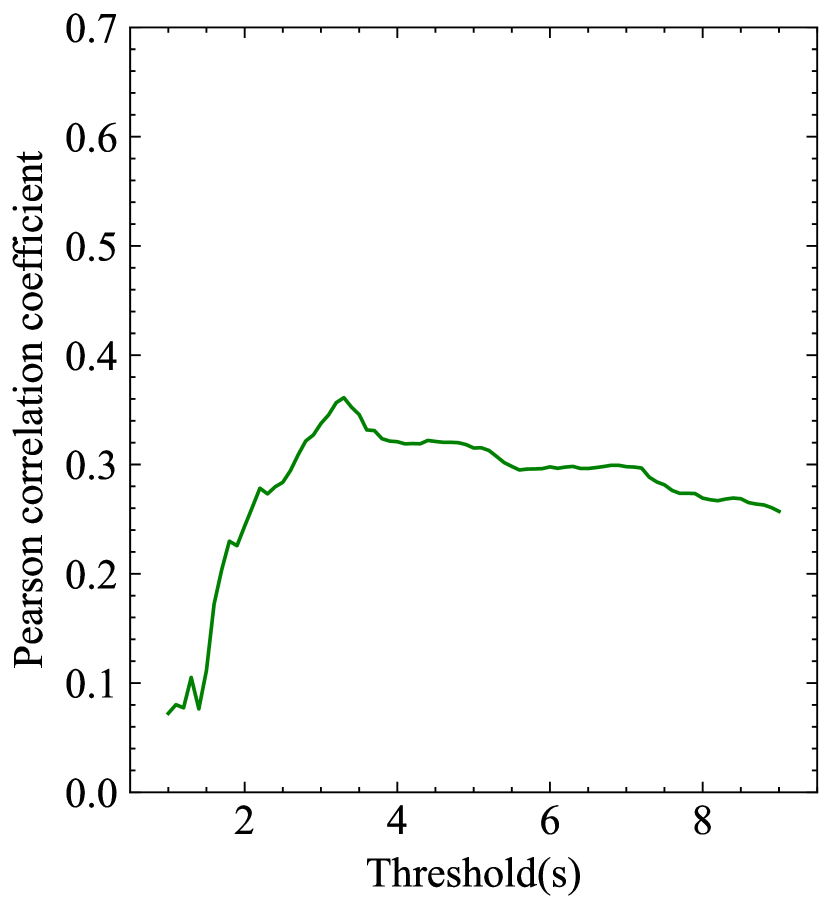
(a) Rear-end risk vs rear-end crash

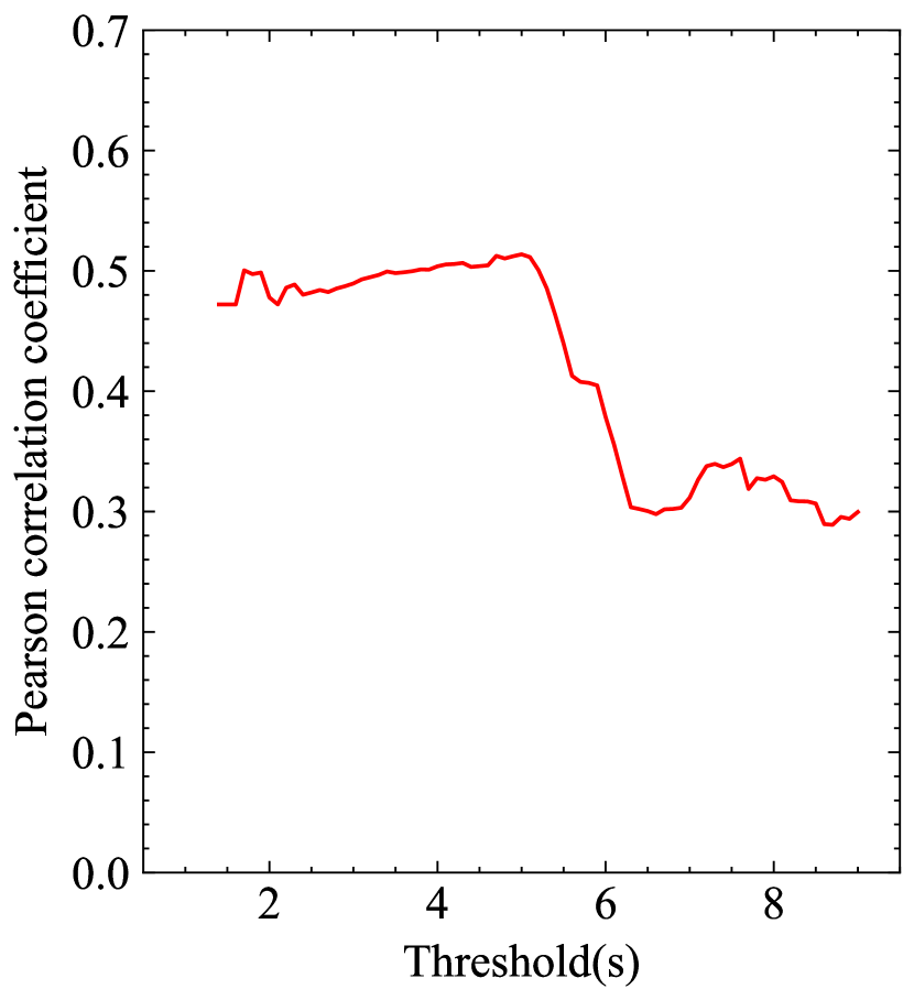
(b) Sideswipe risk vs sideswipe crash

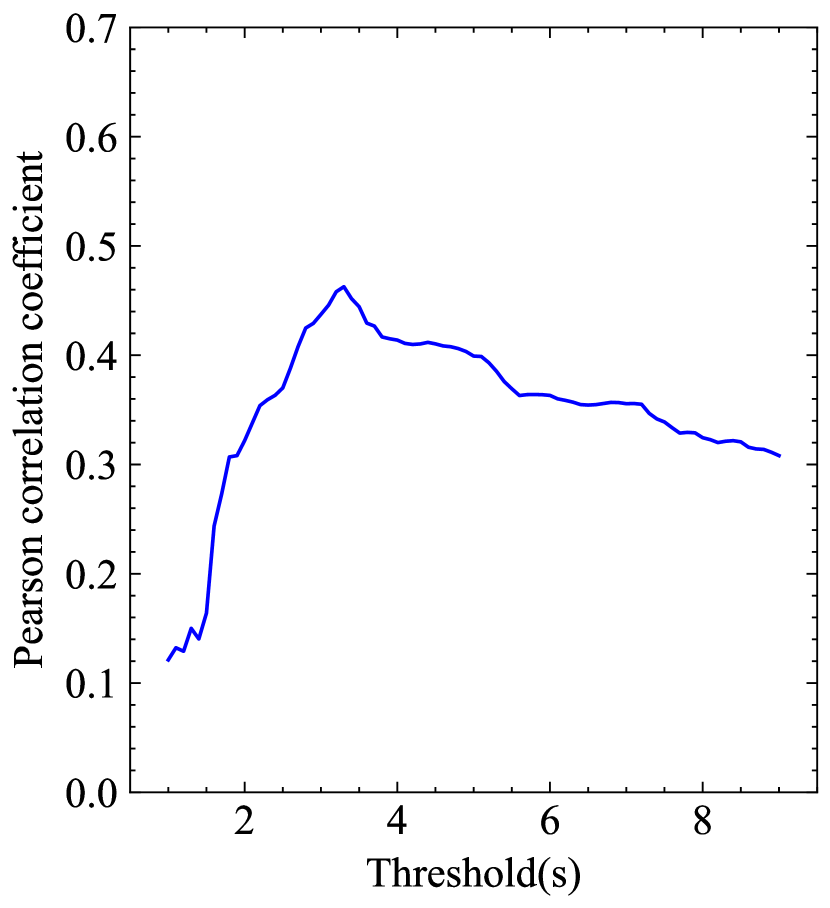
(c) All risk vs all crash

Figure 7: Correlation coefficient between risk rate and crash rate with different combinations

Table 2: Correlation test results

Risk type	Crash type	Optimal threshold(s)	Pearson correlation coefficient	P-value
Rear	Rear	3.3	0.361	0.0015
Sideswipe	Sideswipe	5.0	0.514	0.0000
Rear+sideswipe	Rear+sideswipe	3.3	0.463	0.0000

It is clear that the risks captured during the lane change duration are closely correlated with sideswipe crashes, which are more frequent than rear-end crashes in lane-change-related crashes [Sen et al., 2003]. The highest correlation coefficient 0.514 is obtained between the captured sideswipe risks and the archived sideswipe crashes since the sideswipe crash is closely correlated with the lane change maneuvers. As shown in Table 2, all three p-values are less than 0.05, which indicates the statistically significant correlation between the 2D-TTC and the crashes. The thresholds are also within a reasonable range of common TTC thresholds [Pinnow et al., 2021]. Therefore, the 2D-TTC is a reliable SSM to capture the potential risks in lane change scenarios.

5.2 DDPG model training and results

In this section, the DDPG model was trained with the driving data of safety-critical lane changes. An appropriate pre-specified threshold for 2D-TTC is required to identify and extract the conflicts during lane change maneuvers. In the ADAS applications, the threshold of TTC is usually 5s [Van Der Horst and Hogema, 1993, Scott and Gray, 2008, Mohebbi et al., 2009, Biondi et al., 2017]. The warning is presented as long as the TTC is less than 5s, and the driver is reminded to take evasive actions. Additionally, evasive actions are often found to be executed within a second after the TTC decreases below 5s in the historical (near) crash data [Markkula et al., 2012]. Considering the purpose of this study is to capture and model drivers’ evasive behavior in safety-critical situations, the threshold for 2D-TTC was set to 5s. If there are more than 10 continuous records with 2D-TTC values less than the threshold, it would be regarded as a conflict. After identification and extraction, there were 903 conflicts (lasting for 17,699 time steps) in 743 lane change events. 80% of the data will be used for model training, and the rest 20% are used for model testing.

Three DDPG models, namely the distance (DDPGd), speed (DDPGv), and speed difference (DDPG$\Delta$v) models, were trained using the distance ($R_{d}$), speed ($R_{v}$), and speed difference ($R_{\Delta v}$) rewards, respectively. The input of these models is the observed state at each time step $S_{t}=(d_{lon}(t),v_{lon}(t),\Delta v_{lon}(t),d_{lat}(t),v_{lat}(t),\Delta v_{lat}(t))$, and the outputs of the actor network are the vehicle’s longitudinal and lateral accelerations ($\hat{a}_{lon}$ and $\hat{a}_{lat}$). The DDPG models are expected to learn the underlying policy of driver’s evasive behavior through the interaction with the environment. The architectures of the actor and critic networks are illustrated in Fig. 8. The target actor and critic networks have the same architecture as the actual agent actor and critic networks. The hyperparameters adopted for the DDPG model training are presented in Table 3. Additionally, a neural network (NN) model with two 256-neuron hidden layers was developed as the benchmark for comparison. Its input is the same observed state $S_{t}$ as the DDPG models, and its outputs are also the vehicle’s longitudinal and lateral accelerations ($\hat{a}_{lon}$ and $\hat{a}_{lat}$). The NN model is supposed to imitate the driver’s evasive behaviors in the training set.

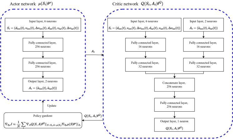
Figure 8: Architectures of the actor and critic networks

Table 3: Hyperparameters in DDPG model

Hyperparameter	Value	Description
Actor learning rate	0.0005	Learning rate used by the Adam optimizer of actor network
Critic learning rate	0.001	Learning rate used by the Adam optimizer of critic network
Discount factor ($\gamma$)	0.9	Discount factor in DDPG
Soft target update rate ($\tau$)	0.01	Soft update rate for target networks
Replay memory size	10,000	Number of training samples in replay memory
Batch size	256	Number of training samples used for gradient update

At the training stage, a safety-critical lane change event was sampled from the training set without replacement and passed to the DDPG model. The model would process the input event sequentially and store the set of experience ($S_{t},A_{t},R_{t},S_{t+1}$) at each time step $t$ in the replay buffer. Then, another event was selected and processed by the DDPG model. If all the events have been used, the training set would be initialized. The training process is repeated for 3,000 episodes, where an episode means loading a safety-critical lane change event. The average episodic reward of the training set with a rolling window of 50 episodes is shown in Fig. 9. All the models start to converge after around 1,500 episodes. The fluctuation at the converged stage is caused by the exploration noises.

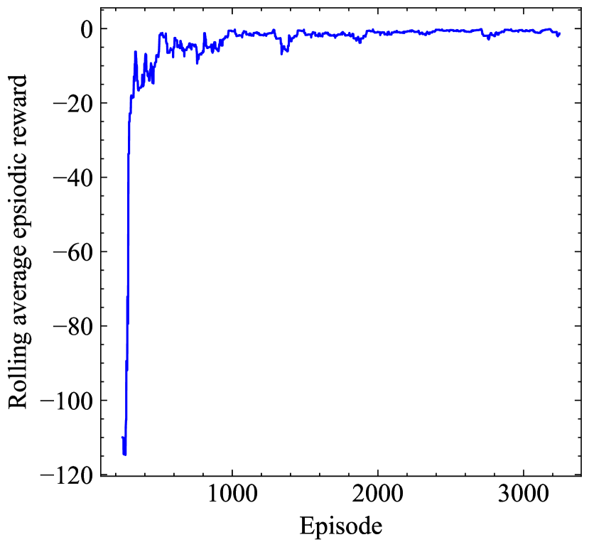
(a) DDPGd model

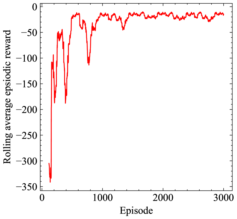
(b) DDPGv model

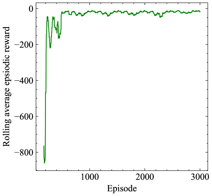
(c) DDPG$\Delta$v model

Figure 9: Rolling average episodic reward of DDPG models on training data

The root mean square error (RMSE) and the Jensen–Shannon divergence (JSD) are employed to evaluate the performances of models in both the longitudinal and lateral motions. The RMSE computes the average error between the simulated and observed values as given by Eq 19.

$$RMSE=\sqrt{\frac{1}{n}\sum_{i=1}^{n}(\hat{x}_{i}-x_{i})^{2}}$$ (19)

where $\hat{x}_{i}$ and $x_{i}$ are the estimated and observed values, respectively. The RMSE of distance ($d_{lon}$ and $d_{lat}$), speed ($v_{lon}$ and $v_{lat}$) and acceleration ($a_{lon}$ and $a_{lat}$) are reported in Table 4. The JSD is used to measure the similarity between the distributions and is also reported in Table 4, which is calculated as

$$JSD(P||Q)=\frac{1}{2}\sum_{x\in\mathcal{X}}P(x)log(\frac{P(x)}{\frac{1}{2}(P(X)+Q(X)})+\frac{1}{2}\sum_{x\in\mathcal{X}}Q(x)log(\frac{Q(x)}{\frac{1}{2}(P(X)+Q(X)})$$ (20)

where $P$ and $Q$ are the estimated and actual discrete probability distributions, respectively.

Table 4: Root mean square error (RMSE) and Jensen–Shannon divergence (JSD) between model results and real data

Variable	DDPGd		DDPGv		DDPG$\Delta$v		NN
	RMSE	JSD	RMSE	JSD	RMSE	JSD	RMSE	JSD
$d_{lon}$	0.0726	0.0006	0.0725*	0.0006*	0.0726	0.0006	0.0728	0.0006
$v_{lon}$	0.0478	0.0008	0.0425*	0.0006*	0.0481	0.0009	0.0539	0.0011
$a_{lon}$	0.4782	0.0182	0.4254*	0.0134*	0.4814	0.0216	0.5392	0.0258
$d_{lat}$	0.0013	0.0013	0.0012	0.0012*	0.0010*	0.0014	0.0013	0.0033
$v_{lat}$	0.0229	0.0042	0.0223*	0.0037*	0.0232	0.0038	0.0235	0.0047
$a_{lat}$	0.2292	0.0138	0.2227*	0.0113*	0.2322	0.0190	0.2354	0.0198

• The best values among all the models.

In general, the proposed DDPG models could capture evasive behaviors accurately. Compared with the baseline NN model, they can achieve better performances in both RMSE and JSD. Because the DRL algorithm can learn the inherent mechanism of the evasive behaviors rather than only imitating them. The NN model becomes less accurate while handling the unseen scenarios in the test set.

Among the DDPG models, the DDPGv model has the lowest RMSE and JSD values on most of the evaluation variables. It outperforms the other two models, especially in terms of longitudinal acceleration. The distributions of the values generated by the DDPGv model are compared with the real data distributions, as shown in Fig. 10. The distributions of the longitudinal and lateral distances, speeds, and accelerations generated by the model are highly consistent with the observed data.

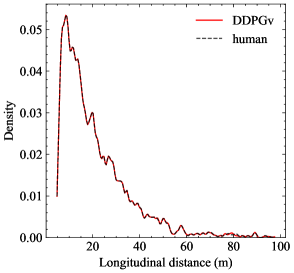
(a) Distribution of longitudinal distance

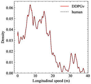
(b) Distribution of longitudinal speed

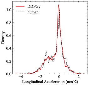
(c) Distribution of longitudinal acceleration

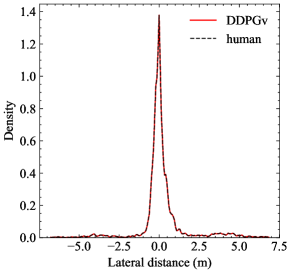
(d) Distribution of lateral distance

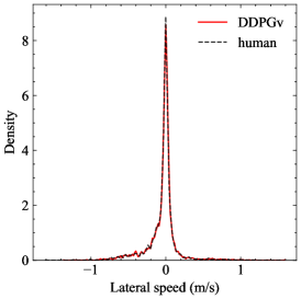
(e) Distribution of lateral speed

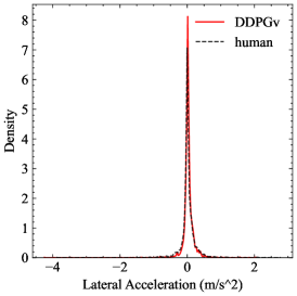
(f) Distribution of lateral acceleration

Figure 10: Distributions of real and estimated values

A possible reason for this performance difference is related to the state updating function, which is given by Eq. 9. The speed of the leading vehicle is assumed to be constant between the observed time $t$ and the simulated time $t+1$. However, the leading vehicle might change its speed in a real situation. The error between the simulated and real values is propagated to the models through the distance and speed difference reward functions (Eq. 10 and Eq. 12. In contrast, the speed reward function (Eq. 11) is only related to the speed of CV and is not influenced by this assumption. Therefore, the accuracies of the DDPGd and DDPG$\Delta$v models are lower than that of the DDPGv model.

5.3 Evasive trajectory simulation

To demonstrate the implementation of the proposed 2D-TTC and DDPG approaches, several safety-critical scenarios were extracted and the evasive trajectories were simulated. Only the initial observed state was given to the models, and the whole trajectory was generated sequentially. The 2D-TTC values during the evasion process were also investigated. The original trajectories of the leading and ego vehicles, the 2D-TTC values, and the simulated longitudinal and lateral movements of the ego vehicle are illustrated in Fig. 11. Specifically, Fig. 11(a), 11(b), and 11(c) demonstrate the situations where the ego vehicles avoid the conflict with cut-in vehicles by changing lanes, and Fig. 11(d) and 11(e) show the cases where the ego vehicles reduce speed as the leading vehicles decelerate.

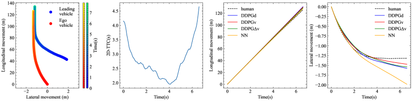
(a) Device=10121, Trip=703, ObstacleId=39

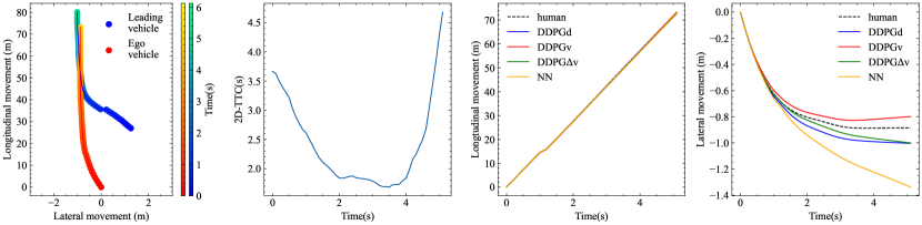
(b) Device=10132, Trip=500, ObstacleId=29

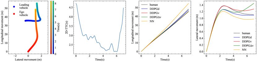
(c) Device=17101, Trip=1039, ObstacleId=15

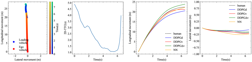
(d) Device=10160, Trip=366, ObstacleId=15

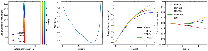
(e) Device=10131, Trip=590, ObstacleId=36

Figure 11: Trajectory reconstruction examples

Overall, the simulated trajectories are highly consistent with the human-driven ones, which indicates that the DDPG algorithms can model both the lane change and deceleration evasive behaviors accurately. The NN model performs worse than the DDPG ones, showing it fails to capture the inherent mechanism of evasive behaviors, and thus it is unable to process the unseen observations in the test set. Among the DDPG models, the DDPGv model predicts the trajectories closest to the observed ones in most cases.

Besides, the 2D-TTC method can detect potential conflict in various situations precisely. The U-shaped 2D-TTC curve shows its ability to reflect the process of evasive behavior, from the danger realization to the successful collision avoidance. It is worth to mention that the 2D-TTC start from a value less than the set threshold in some cases, especially when the leading vehicle cuts in from another lane within a short distance. Because the view angle of the MobilEye main camera is $28^{\circ}$ [Stein et al., 2003], the conflict cannot be captured until the leading vehicle enters the detection range. However, the trajectory suggests that the driver might realize the conflict before it is detected by the sensor and took evasive action.

6 Conclusion

In this study, DDPG-based driver’s evasive behavior models during safety-critical lane changes were developed using the large-scale driving data collected by CVs. A novel 2D-TTC was proposed to capture the potential risks and identify safety-critical lane changes. It is capable to detect the risks in 2D traffic scenarios without the need for complete trajectories and is suitable for real-time risk estimation using the data collected by CVs. The correlation between the conflicts identified by 2D-TTC and the historical crashes was investigated. The results show that the risks captured by the 2D-TTC are highly correlated with the archived crashes. Furthermore, a DDPG-based evasive behavior model was developed based on the safety-critical situations detected by the 2D-TTC measure. The results indicate that the DDPG model can model both the longitudinal and lateral evasive behaviors accurately, and the simulated trajectories are highly consistent with the actual ones. The DDPG model also shows superior performance in understanding the conflict evasion strategies and predicting the precise trajectories compared to the conventional NN model. The evasive behavior model could facilitate the development of safety-aware microscopic simulations and predictive collision avoidance systems. For future studies, the transferability of the proposed methods will be further tested using the datasets in different driving environments.

References

- Abdulhai and Kattan [2003] Abdulhai, B., Kattan, L., 2003. Reinforcement learning: Introduction to theory and potential for transport applications. Canadian Journal of Civil Engineering 30, 981–991.
- Ali et al. [2020] Ali, Y., Bliemer, M.C., Zheng, Z., Haque, M.M., 2020. Cooperate or not? exploring drivers’ interactions and response times to a lane-changing request in a connected environment. Transportation Research Part C: Emerging Technologies 120, 102816.
- Alsaleh and Sayed [2021] Alsaleh, R., Sayed, T., 2021. Markov-game modeling of cyclist-pedestrian interactions in shared spaces: A multi-agent adversarial inverse reinforcement learning approach. Transportation research part C: emerging technologies 128, 103191.
- Aslani et al. [2017] Aslani, M., Mesgari, M.S., Wiering, M., 2017. Adaptive traffic signal control with actor-critic methods in a real-world traffic network with different traffic disruption events. Transportation Research Part C: Emerging Technologies 85, 732–752.
- Bezzina and Sayer [2014] Bezzina, D., Sayer, J., 2014. Safety pilot model deployment: Test conductor team report. Technical Report DOT HS 812 171. National Highway Traffic Safety Administration.
- Biondi et al. [2017] Biondi, F., Strayer, D.L., Rossi, R., Gastaldi, M., Mulatti, C., 2017. Advanced driver assistance systems: Using multimodal redundant warnings to enhance road safety. Applied ergonomics 58, 238–244.
- Chae et al. [2017] Chae, H., Kang, C.M., Kim, B., Kim, J., Chung, C.C., Choi, J.W., 2017. Autonomous braking system via deep reinforcement learning, in: 2017 IEEE 20th International conference on intelligent transportation systems (ITSC), IEEE. pp. 1–6.
- Chen et al. [2021] Chen, Q., Huang, H., Li, Y., Lee, J., Long, K., Gu, R., Zhai, X., 2021. Modeling accident risks in different lane-changing behavioral patterns. Analytic methods in accident research 30, 100159.
- Deveaux et al. [2021] Deveaux, D., Higuchi, T., Uçar, S., Wang, C.H., Härri, J., Altintas, O., 2021. Extraction of risk knowledge from time to collision variation in roundabouts, in: 2021 IEEE International Intelligent Transportation Systems Conference (ITSC), IEEE. pp. 3665–3672.
- Dong et al. [2021] Dong, J., Chen, S., Li, Y., Du, R., Steinfeld, A., Labi, S., 2021. Space-weighted information fusion using deep reinforcement learning: The context of tactical control of lane-changing autonomous vehicles and connectivity range assessment. Transportation Research Part C: Emerging Technologies 128, 103192.
- Dozza [2013] Dozza, M., 2013. What factors influence drivers’ response time for evasive maneuvers in real traffic? Accident Analysis & Prevention 58, 299–308.
- ESRI [2011] ESRI, 2011. ArcGIS Desktop: Release 10. Environmental Systems Research Institute, Redlands, CA.
- Essa and Sayed [2020] Essa, M., Sayed, T., 2020. Self-learning adaptive traffic signal control for real-time safety optimization. Accident Analysis & Prevention 146, 105713.
- Farazi et al. [2021] Farazi, N.P., Zou, B., Ahamed, T., Barua, L., 2021. Deep reinforcement learning in transportation research: A review. Transportation research interdisciplinary perspectives 11, 100425.
- Gettman and Head [2003] Gettman, D., Head, L., 2003. Surrogate safety measures from traffic simulation models. Transportation Research Record 1840, 104–115.
- Guo et al. [2022] Guo, H., Keyvan-Ekbatani, M., Xie, K., 2022. Lane change detection and prediction using real-world connected vehicle data. Transportation Research Part C: Emerging Technologies 142, 103785.
- Guo et al. [2021] Guo, H., Xie, K., Keyvan-Ekbatani, M., 2021. Lane change detection using naturalistic driving data, in: 2021 7th International Conference on Models and Technologies for Intelligent Transportation Systems (MT-ITS), IEEE. pp. 1–6.
- Hamilton and Allen [2015] Hamilton, B., Allen, 2015. Safety pilot model deployment-sample data environment data handbook. Technical Report. US department of transportation.
- Happee et al. [2017] Happee, R., Gold, C., Radlmayr, J., Hergeth, S., Bengler, K., 2017. Take-over performance in evasive manoeuvres. Accident Analysis & Prevention 106, 211–222.
- Harding et al. [2014] Harding, J., Powell, G., Yoon, R., Fikentscher, J., Doyle, C., Sade, D., Lukuc, M., Simons, J., Wang, J., et al., 2014. Vehicle-to-vehicle communications: readiness of V2V technology for application. Technical Report DOT HS 812 014. National Highway Traffic Safety Administration.
- Haydari and Yilmaz [2020] Haydari, A., Yilmaz, Y., 2020. Deep reinforcement learning for intelligent transportation systems: A survey. IEEE Transactions on Intelligent Transportation Systems .
- Hayward [1972] Hayward, J.C., 1972. Near miss determination through use of a scale of danger. Transportation Research Record , 24–34.
- Henclewood et al. [2014] Henclewood, D., Abramovich, M., Yelchuru, B., 2014. Safety pilot model deployment–one day sample data environment data handbook. Technical Report. Research and Technology Innovation Administration, US Department of Transportation.
- Horiuchi et al. [2001] Horiuchi, S., Okada, K., Nohtomi, S., 2001. Numerical analysis of optimal vehicle trajectories for emergency obstacle avoidance. JSAE review 22, 495–502.
- Hou et al. [2014] Hou, J., List, G.F., Guo, X., 2014. New algorithms for computing the time-to-collision in freeway traffic simulation models. Computational intelligence and neuroscience 2014.
- Huang et al. [2018] Huang, X., Sun, J., Sun, J., 2018. A car-following model considering asymmetric driving behavior based on long short-term memory neural networks. Transportation research part C: emerging technologies 95, 346–362.
- Huang et al. [2017] Huang, X., Zhao, D., Peng, H., 2017. Empirical study of dsrc performance based on safety pilot model deployment data. IEEE Transactions on Intelligent Transportation Systems 18, 2619–2628.
- Jamson et al. [2013] Jamson, A.H., Merat, N., Carsten, O.M., Lai, F.C., 2013. Behavioural changes in drivers experiencing highly-automated vehicle control in varying traffic conditions. Transportation research part C: emerging technologies 30, 116–125.
- Jurecki and Stańczyk [2009] Jurecki, R., Stańczyk, T., 2009. Driver model for the analysis of pre-accident situations. Vehicle System Dynamics 47, 589–612.
- Kelly Blue Book [2013] Kelly Blue Book, 2013. Highest horsepower sedans of 2013. https://www.kbb.com/highest-horsepower-cars/sedan/2013/.
- Keyvan-Ekbatani et al. [2016] Keyvan-Ekbatani, M., Knoop, V.L., Daamen, W., 2016. Categorization of the lane change decision process on freeways. Transportation research part C: emerging technologies 69, 515–526.
- Kuang et al. [2015] Kuang, Y., Qu, X., Wang, S., 2015. A tree-structured crash surrogate measure for freeways. Accident Analysis & Prevention 77, 137–148.
- Lee et al. [2019] Lee, S., Ngoduy, D., Keyvan-Ekbatani, M., 2019. Integrated deep learning and stochastic car-following model for traffic dynamics on multi-lane freeways. Transportation research part C: emerging technologies 106, 360–377.
- Lenard et al. [2018] Lenard, J., Welsh, R., Danton, R., 2018. Time-to-collision analysis of pedestrian and pedal-cycle accidents for the development of autonomous emergency braking systems. Accident Analysis & Prevention 115, 128–136.
- Li et al. [2022] Li, G., Yang, Y., Li, S., Qu, X., Lyu, N., Li, S.E., 2022. Decision making of autonomous vehicles in lane change scenarios: Deep reinforcement learning approaches with risk awareness. Transportation research part C: emerging technologies 134, 103452.
- Li [2017] Li, Y., 2017. Deep reinforcement learning: An overview. arXiv preprint arXiv:1701.07274 .
- Li et al. [2017] Li, Y., Wang, H., Wang, W., Xing, L., Liu, S., Wei, X., 2017. Evaluation of the impacts of cooperative adaptive cruise control on reducing rear-end collision risks on freeways. Accident Analysis & Prevention 98, 87–95.
- Li et al. [2021] Li, Y., Wu, D., Chen, Q., Lee, J., Long, K., 2021. Exploring transition durations of rear-end collisions based on vehicle trajectory data: a survival modeling approach. Accident Analysis & Prevention 159, 106271.
- Li et al. [2020] Li, Y., Wu, D., Lee, J., Yang, M., Shi, Y., 2020. Analysis of the transition condition of rear-end collisions using time-to-collision index and vehicle trajectory data. Accident Analysis & Prevention 144, 105676.
- Lillicrap et al. [2015] Lillicrap, T.P., Hunt, J.J., Pritzel, A., Heess, N., Erez, T., Tassa, Y., Silver, D., Wierstra, D., 2015. Continuous control with deep reinforcement learning. arXiv preprint arXiv:1509.02971 .
- Ma and Qu [2020] Ma, L., Qu, S., 2020. A sequence to sequence learning based car-following model for multi-step predictions considering reaction delay. Transportation research part C: emerging technologies 120, 102785.
- Ma and Ahn [2008] Ma, T., Ahn, S., 2008. Comparisons of speed-spacing relations under general car following versus lane changing. Transportation research record 2088, 138–147.
- Markkula [2014] Markkula, G., 2014. Modeling driver control behavior in both routine and near-accident driving, in: Proceedings of the human factors and ergonomics society annual meeting, SAGE Publications Sage CA: Los Angeles, CA. pp. 879–883.
- Markkula et al. [2012] Markkula, G., Benderius, O., Wolff, K., Wahde, M., 2012. A review of near-collision driver behavior models. Human factors 54, 1117–1143.
- Markkula et al. [2016] Markkula, G., Engström, J., Lodin, J., Bärgman, J., Victor, T., 2016. A farewell to brake reaction times? kinematics-dependent brake response in naturalistic rear-end emergencies. Accident Analysis & Prevention 95, 209–226.
- McGehee et al. [1999] McGehee, D.V., Mazzae, E.N., Baldwin, G.S., Grant, P., Simmons, C.J., Hankey, J., Forkenbrock, G., 1999. Examination of drivers’ collision avoidance behavior using conventional and antilock brake systems on the iowa driving simulator. Technical Report. University of Iowa.
- Minderhoud and Bovy [2001] Minderhoud, M.M., Bovy, P.H., 2001. Extended time-to-collision measures for road traffic safety assessment. Accident Analysis & Prevention 33, 89–97.
- Mnih et al. [2015] Mnih, V., Kavukcuoglu, K., Silver, D., Rusu, A.A., Veness, J., Bellemare, M.G., Graves, A., Riedmiller, M., Fidjeland, A.K., Ostrovski, G., et al., 2015. Human-level control through deep reinforcement learning. nature 518, 529–533.
- Mohebbi et al. [2009] Mohebbi, R., Gray, R., Tan, H.Z., 2009. Driver reaction time to tactile and auditory rear-end collision warnings while talking on a cell phone. Human factors 51, 102–110.
- Najm et al. [2013] Najm, W.G., Ranganathan, R., Srinivasan, G., Smith, J.D., Toma, S., Swanson, E., Burgett, A., et al., 2013. Description of light-vehicle pre-crash scenarios for safety applications based on vehicle-to-vehicle communications. Technical Report. United States. National Highway Traffic Safety Administration.
- Nasernejad et al. [2021] Nasernejad, P., Sayed, T., Alsaleh, R., 2021. Modeling pedestrian behavior in pedestrian-vehicle near misses: A continuous gaussian process inverse reinforcement learning (gp-irl) approach. Accident Analysis & Prevention 161, 106355.
- Ozan et al. [2015] Ozan, C., Baskan, O., Haldenbilen, S., Ceylan, H., 2015. A modified reinforcement learning algorithm for solving coordinated signalized networks. Transportation Research Part C: Emerging Technologies 54, 40–55.
- Ozbay et al. [2008] Ozbay, K., Yang, H., Bartin, B., Mudigonda, S., 2008. Derivation and validation of new simulation-based surrogate safety measure. Transportation research record 2083, 105–113.
- Papini et al. [2021] Papini, G.P.R., Plebe, A., Da Lio, M., Donà, R., 2021. A reinforcement learning approach for enacting cautious behaviours in autonomous driving system: Safe speed choice in the interaction with distracted pedestrians. IEEE Transactions on Intelligent Transportation Systems .
- Pearson [1895] Pearson, K., 1895. Vii. note on regression and inheritance in the case of two parents. proceedings of the royal society of London 58, 240–242.
- Petersen and Barrett [2009] Petersen, A., Barrett, R., 2009. Postural stability and vehicle kinematics during an evasive lane change manoeuvre: A driver training study. Ergonomics 52, 560–568.
- Pinnow et al. [2021] Pinnow, J., Masoud, M., Elhenawy, M., Glaser, S., 2021. A review of naturalistic driving study surrogates and surrogate indicator viability within the context of different road geometries. Accident Analysis & Prevention 157, 106185.
- Sarkar et al. [2021] Sarkar, A., Hickman, J.S., McDonald, A.D., Huang, W., Vogelpohl, T., Markkula, G., 2021. Steering or braking avoidance response in shrp2 rear-end crashes and near-crashes: A decision tree approach. Accident Analysis & Prevention 154, 106055.
- Scanlon et al. [2021] Scanlon, J.M., Kusano, K.D., Daniel, T., Alderson, C., Ogle, A., Victor, T., 2021. Waymo simulated driving behavior in reconstructed fatal crashes within an autonomous vehicle operating domain. Accident Analysis & Prevention 163, 106454.
- Scanlon et al. [2015] Scanlon, J.M., Kusano, K.D., Gabler, H.C., 2015. Analysis of driver evasive maneuvering prior to intersection crashes using event data recorders. Traffic injury prevention 16, S182–S189.
- Schmidt et al. [2006] Schmidt, C., Oechsle, F., Branz, W., 2006. Research on trajectory planning in emergency situations with multiple objects, in: 2006 IEEE Intelligent Transportation Systems Conference, IEEE. pp. 988–992.
- Schnelle et al. [2018] Schnelle, S., Wang, J., Jagacinski, R., Su, H.j., 2018. A feedforward and feedback integrated lateral and longitudinal driver model for personalized advanced driver assistance systems. Mechatronics 50, 177–188.
- Scott and Gray [2008] Scott, J., Gray, R., 2008. A comparison of tactile, visual, and auditory warnings for rear-end collision prevention in simulated driving. Human factors 50, 264–275.
- Sen et al. [2003] Sen, B., Smith, J.D., Najm, W.G., et al., 2003. Analysis of lane change crashes. Technical Report. United States. National Highway Traffic Safety Administration.
- Shi et al. [2021] Shi, H., Zhou, Y., Wu, K., Wang, X., Lin, Y., Ran, B., 2021. Connected automated vehicle cooperative control with a deep reinforcement learning approach in a mixed traffic environment. Transportation Research Part C: Emerging Technologies 133, 103421.
- Shibata et al. [2014] Shibata, N., Sugiyama, S., Wada, T., 2014. Collision avoidance control with steering using velocity potential field, in: 2014 IEEE Intelligent Vehicles Symposium Proceedings, IEEE. pp. 438–443.
- Silver et al. [2014] Silver, D., Lever, G., Heess, N., Degris, T., Wierstra, D., Riedmiller, M., 2014. Deterministic policy gradient algorithms, in: International conference on machine learning, PMLR. pp. 387–395.
- Soudbakhsh et al. [2011] Soudbakhsh, D., Eskandarian, A., Moreau, J., 2011. An emergency evasive maneuver algorithm for vehicles, in: 2011 14th International IEEE Conference on Intelligent Transportation Systems (ITSC), IEEE. pp. 973–978.
- Stein et al. [2003] Stein, G.P., Mano, O., Shashua, A., 2003. Vision-based acc with a single camera: bounds on range and range rate accuracy, in: IEEE IV2003 intelligent vehicles symposium. Proceedings (Cat. No. 03TH8683), IEEE. pp. 120–125.
- Sugimoto and Sauer [2005] Sugimoto, Y., Sauer, C., 2005. Effectiveness estimation method for advanced driver assistance system and its application to collision mitigation brake system, in: Proceedings of the 19th International Technical Conference on the Enhanced Safety of Vehicles, National Highway Traffic Safety Administration Washington, DC.
- Sun and Kondyli [2010] Sun, D., Kondyli, A., 2010. Modeling vehicle interactions during lane-changing behavior on arterial streets. Computer-Aided Civil and Infrastructure Engineering 25, 557–571.
- Svärd et al. [2021] Svärd, M., Markkula, G., Bärgman, J., Victor, T., 2021. Computational modeling of driver pre-crash brake response, with and without off-road glances: Parameterization using real-world crashes and near-crashes. Accident Analysis & Prevention 163, 106433.
- Svärd et al. [2017] Svärd, M., Markkula, G., Engström, J., Granum, F., Bärgman, J., 2017. A quantitative driver model of pre-crash brake onset and control, in: Proceedings of the Human Factors and Ergonomics Society Annual Meeting, SAGE Publications Sage CA: Los Angeles, CA. pp. 339–343.
- Tian et al. [2021] Tian, Y., Cao, X., Huang, K., Fei, C., Zheng, Z., Ji, X., 2021. Learning to drive like human beings: A method based on deep reinforcement learning. IEEE Transactions on Intelligent Transportation Systems .
- Tseng et al. [2005] Tseng, H., Asgari, J., Hrovat, D., Van Der Jagt, P., Cherry, A., Neads, S., 2005. Evasive manoeuvres with a steering robot. Vehicle system dynamics 43, 199–216.
- Uhlenbeck and Ornstein [1930] Uhlenbeck, G.E., Ornstein, L.S., 1930. On the theory of the brownian motion. Physical review 36, 823.
- Van Der Horst and Hogema [1993] Van Der Horst, R., Hogema, J., 1993. Time-to-collision and collision avoidance systems .
- Van Rossum and Drake [2009] Van Rossum, G., Drake, F.L., 2009. Python 3 Reference Manual. CreateSpace, Scotts Valley, CA.
- Venkatraman et al. [2016] Venkatraman, V., Lee, J.D., Schwarz, C.W., 2016. Steer or brake?: Modeling drivers’ collision-avoidance behavior by using perceptual cues. Transportation research record 2602, 97–103.
- Venthuruthiyil and Chunchu [2022] Venthuruthiyil, S.P., Chunchu, M., 2022. Anticipated collision time (act): A two-dimensional surrogate safety indicator for trajectory-based proactive safety assessment. Transportation Research Part C: Emerging Technologies 139, 103655.
- Wang and Coifman [2008] Wang, C., Coifman, B., 2008. The effect of lane-change maneuvers on a simplified car-following theory. IEEE transactions on intelligent transportation systems 9, 523–535.
- Wang et al. [2018] Wang, C., Xu, C., Xia, J., Qian, Z., Lu, L., 2018. A combined use of microscopic traffic simulation and extreme value methods for traffic safety evaluation. Transportation Research Part C: Emerging Technologies 90, 281–291.
- Wang et al. [2021] Wang, G., Hu, J., Li, Z., Li, L., 2021. Harmonious lane changing via deep reinforcement learning. IEEE Transactions on Intelligent Transportation Systems .
- Ward et al. [2015] Ward, J.R., Agamennoni, G., Worrall, S., Bender, A., Nebot, E., 2015. Extending time to collision for probabilistic reasoning in general traffic scenarios. Transportation Research Part C: Emerging Technologies 51, 66–82.
- Xie et al. [2016] Xie, K., Li, C., Ozbay, K., Dobler, G., Yang, H., Chiang, A.T., Ghandehari, M., 2016. Development of a comprehensive framework for video-based safety assessment, in: 2016 IEEE 19th International Conference on Intelligent Transportation Systems (ITSC), IEEE. pp. 2638–2643.
- Xie et al. [2019] Xie, K., Yang, D., Ozbay, K., Yang, H., 2019. Use of real-world connected vehicle data in identifying high-risk locations based on a new surrogate safety measure. Accident Analysis & Prevention 125, 311–319.
- Xing et al. [2019] Xing, L., He, J., Abdel-Aty, M., Cai, Q., Li, Y., Zheng, O., 2019. Examining traffic conflicts of up stream toll plaza area using vehicles’ trajectory data. Accident Analysis & Prevention 125, 174–187.
- Xing et al. [2020] Xing, Y., Lv, C., Wang, H., Cao, D., Velenis, E., 2020. An ensemble deep learning approach for driver lane change intention inference. Transportation Research Part C: Emerging Technologies 115, 102615.
- Xiong et al. [2019] Xiong, X., Wang, M., Cai, Y., Chen, L., Farah, H., Hagenzieker, M., 2019. A forward collision avoidance algorithm based on driver braking behavior. Accident Analysis & Prevention 129, 30–43.
- Xu et al. [2012] Xu, G., Liu, L., Ou, Y., Song, Z., 2012. Dynamic modeling of driver control strategy of lane-change behavior and trajectory planning for collision prediction. IEEE Transactions on Intelligent Transportation Systems 13, 1138–1155.
- Xue et al. [2018] Xue, Q., Markkula, G., Yan, X., Merat, N., 2018. Using perceptual cues for brake response to a lead vehicle: Comparing threshold and accumulator models of visual looming. Accident Analysis & Prevention 118, 114–124.
- Yang et al. [2021a] Yang, D., Ozbay, K., Xie, K., Yang, H., Zuo, F., Sha, D., 2021a. Proactive safety monitoring: A functional approach to detect safety-related anomalies using unmanned aerial vehicle video data. Transportation research part C: emerging technologies 127, 103130.
- Yang et al. [2021b] Yang, D., Xie, K., Ozbay, K., Yang, H., 2021b. Fusing crash data and surrogate safety measures for safety assessment: Development of a structural equation model with conditional autoregressive spatial effect and random parameters. Accident Analysis & Prevention 152, 105971.
- Ye et al. [2019] Ye, Y., Zhang, X., Sun, J., 2019. Automated vehicle’s behavior decision making using deep reinforcement learning and high-fidelity simulation environment. Transportation Research Part C: Emerging Technologies 107, 155–170.
- Yuan et al. [2019] Yuan, H., Sun, X., Gordon, T., 2019. Unified decision-making and control for highway collision avoidance using active front steer and individual wheel torque control. Vehicle system dynamics 57, 1188–1205.
- Zaharia et al. [2016] Zaharia, M., Xin, R.S., Wendell, P., Das, T., Armbrust, M., Dave, A., Meng, X., Rosen, J., Venkataraman, S., Franklin, M.J., et al., 2016. Apache spark: a unified engine for big data processing. Communications of the ACM 59, 56–65.
- Zhang et al. [2021] Zhang, C., Zhu, J., Wang, W., Xi, J., 2021. Spatiotemporal learning of multivehicle interaction patterns in lane-change scenarios. IEEE Transactions on Intelligent Transportation Systems .
- Zhao et al. [2017] Zhao, D., Guo, Y., Jia, Y.J., 2017. Trafficnet: An open naturalistic driving scenario library, in: 2017 IEEE 20th International Conference on Intelligent Transportation Systems (ITSC), IEEE. pp. 1–8.
- Zheng et al. [2020] Zheng, L., Zeng, P., Yang, W., Li, Y., Zhan, Z., 2020. Bézier curve-based trajectory planning for autonomous vehicles with collision avoidance. IET Intelligent Transport Systems 14, 1882–1891.
- Zheng [2014] Zheng, Z., 2014. Recent developments and research needs in modeling lane changing. Transportation research part B: methodological 60, 16–32.
- Zheng et al. [2013] Zheng, Z., Ahn, S., Chen, D., Laval, J., 2013. The effects of lane-changing on the immediate follower: Anticipation, relaxation, and change in driver characteristics. Transportation research part C: emerging technologies 26, 367–379.
- Zheng et al. [2010] Zheng, Z., Ahn, S., Monsere, C.M., 2010. Impact of traffic oscillations on freeway crash occurrences. Accident Analysis & Prevention 42, 626–636.
- Zhou and Zhong [2020] Zhou, H., Zhong, Z., 2020. Evasive behavior-based method for threat assessment in different scenarios: A novel framework for intelligent vehicle. Accident Analysis & Prevention 148, 105798.
- Zhu et al. [2018] Zhu, M., Wang, X., Wang, Y., 2018. Human-like autonomous car-following model with deep reinforcement learning. Transportation research part C: emerging technologies 97, 348–368.
- Zhu et al. [2020] Zhu, M., Wang, Y., Pu, Z., Hu, J., Wang, X., Ke, R., 2020. Safe, efficient, and comfortable velocity control based on reinforcement learning for autonomous driving. Transportation Research Part C: Emerging Technologies 117, 102662.
- Zuo et al. [2020] Zuo, F., Ozbay, K., Kurkcu, A., Gao, J., Yang, H., Xie, K., 2020. Microscopic simulation based study of pedestrian safety applications at signalized urban crossings in a connected-automated vehicle environment and reinforcement learning based optimization of vehicle decisions. Advances in transportation studies .