Absorption lines from magnetically driven winds in X-ray binaries II: high resolution observational signatures expected from future X-ray observatories

Abstract

In our self-similar, analytical, magneto-hydrodynamic (MHD) accretion-ejection solution, the density at the base of the outflow is explicitly dependent on the disk accretion rate – a unique property of this class of solutions. We had earlier found that the ejection index $p>\sim 0.1(\dot{M}_{acc}\propto r^{p})$ is a key MHD parameter that decides if the flow can cause absorption lines in the high resolution X-ray spectra of black hole binaries. Here we choose 3 dense warm solutions with $p=0.1,0.3,0.45$ and carefully develop a methodology to generate spectra which are convolved with the Athena and XRISM response functions to predict what they will observe seeing through such MHD outflows. In this paper two other external parameters were varied - extent of the disk, $\rm{r_{o}|_{max}}=10^{5},\,10^{6}\,\,\rm{r_{G}}$, and the angle of the line of sight, $i\sim 10-25^{\circ}$. Resultant absorption lines (H and He-like Fe, Ca, Ar) change in strength and their profiles manifest varying degrees of asymmetry. We checked if a) the lines and ii) the line asymmetries are detected, in our suit of synthetic Athena and XRISM spectra. Our analysis shows that Athena should detect the lines and their asymmetries for a standard 100 ksec observation of a 100 mCrab source - lines with equivalent width as low as a few eV should be detected if the 6-8 keV counts are larger than $10^{4}-10^{5}$ even for the least favourable simulated cases.

1 Introduction

High resolution soft X-ray spectra from Chandra and XMM-Newton show blueshifted absorption line when observing some stellar mass black holes in binary systems (black hole binaries, hereafter BHBs). These lines are signatures of winds from the accretion disk around the black hole. The velocity and ionization state of the gas interpreted from the absorption lines vary from object to object and from observation to observation. In most cases, we see lines only from H- and He-like Fe ions (e.g. Lee et al. 2002, Neilsen & Lee 2009 with GRS 1915+105, Miller et al. 2004 with GX 339-4, Miller et al. 2006 with H1743-322, and King et al. 2012 with IGR J17091-3624). Some spectra of some of the objects, however, display lines from a wider range of ions from O through Fe (e.g. Ueda et al. 2009 for GRS 1915+105, Miller et al. 2008; Kallman et al. 2009 for GRO J1655–40). The variations in the wind properties seem to indicate variations in the temperature, pressure, and density of the gas, not only from one object to another, but also from one spectrum of the same object to another spectrum, depending on the accretion state of the black hole.

The spectral energy distributions (SEDs) of BHBs in the different accretion states have varying degrees of contribution from the accretion disk and the non-thermal power-law components. The winds are not present in all the states. The absorption lines are more prominent in the Softer (accretion disk dominated) states (Miller et al., 2008; Neilsen & Lee, 2009; Blum et al., 2010; Ponti et al., 2012). Some authors (e.g. Miller et al., 2012, in the case of H1743-322) show that the changing photoionising flux is responsible for the variation in the wind strength; others conjecture that the underlying outflowing gas changes its physical properties.

The observable properties of the accretion disk winds are often used to infer the driving mechanism of the winds (Lee et al., 2002; Ueda et al., 2009, 2010; Neilsen et al., 2011; Neilsen & Homan, 2012). So, the changes in the wind (or its disappearance) through the various states of the BHB, has been interpreted as a variation in the driving mechanism. To elaborate, let us use the case of GRO J1655–40. A well-known Chandra observation of GRO J1655–40 (Miller et al., 2006, 2008; Kallman et al., 2009) shows a rich absorption line spectrum from OVIII - NiXXVI, which led the authors to conclude that a magnetic driving mechanism is accelerating the wind. Neilsen & Homan (2012) have analysed the data from another observation for the same source taken three weeks later and found absorption lines from only Fe  xxvi! It was shown that such a change in the wind was not due to mere change in photoionization flux. The disappearance of most of the absorption lines suggest that in the wind in GRO J1655–40, the long term changes may be driven by the variations in the thermal pressure and/or magnetic fields. This wind was hailed to be the most convincing evidence for magnetic driving in BHBs. Since the spectrum of GRO J1655-40 with this wide range of ions, is a unique one among BHBs, it is repeatedly investigated by different authors. More recently, Neilsen et al. (2016) and Shidatsu, Done & Ueda (2016) have studied the same spectrum. Both papers use complimentary optical and near-infrared observations around the Chandra observations and hypothesise the presence of a Compton-thick, almost completely ionized, gas component which caused scattering and hence caused reduction in the observed X-ray luminosity. These conjectures point to the possibility of a near Eddington flow, whence radiation pressure and Compton heating may be significant contributors to the wind that has been hailed to be a magnetically driven wind.

In order to have a consolidated picture of these systems, it is necessary to understand the relation between the accretion states of the BHBs and the driving mechanisms of the winds. In Chakravorty et al. (2016, hereafter called Paper I), we have investigated the magneto-hydrodynamic (hereafter MHD) solutions as driving mechanisms for winds from the accretion disks around BHBs: cold solutions (with no disk surface heating) from Ferreira (1997, hereafter F97) and warm solutions (which involve an ad-hoc disk surface heating term) from Casse & Ferreira (2000b) and Ferreira (2004). We had concluded that only the warm class of solutions, which have heating at the disk surface, can have sufficiently high values of the ejection efficiency $p(\gtrsim 0.1)$ so that the winds are dense enough to explain the observed absorption lines and the inferred physical properties. However, since then it was possible to investigate the variations in the disk magnetisations more elaborately. Jacquemin-Ide, Ferreira & Lesur (2019) have derived cold MHD solutions with $p(\sim 0.1)$, but magnetisation very different from the ones in Paper I. Further, their analysis showed that $p$ can go as high as $\sim 0.2-0.3$ for weakly magnetised solutions.

In Paper I, we published the important physical properties of the gas, for example, the density and velocity of the flow and specified the regions which would have the correct ionisation properties to yield FeXXVI absorption lines. In this paper we are taking the next crucial step - producing synthetic spectra which can be matched to observations from current (Chandra) and future (XRISM and Athena) missions. The goal of this paper is to set up a methodology of looking for the ‘correct’ MHD outflow models within our suite of solutions, based on the observable line profiles that they produce. We want to study the variation of the line profiles as functions of the physical properties like the line-of-sight (LOS) angle (i, from the surface of the disk), the ejection index (p), the extent of the disk. We intend this paper to be the 1st among a list of publications where we shall look at the details of the observables (e.g. the Fe XXVI K$\alpha$ doublet line profiles) in a X-ray spectra and how they are related to the MHD outflow model parameters, including some of the disk parameters like the ejection index and the disk magnetisation. The intention is to have an uniform, systematic study of a suite of MHD models, and not just a preferred few to suit specific observed spectrum. This long term project would be an attempt to build a library of models that can be tested out (against other non-magnetic driving mechanisms) using the XRISM and Athena spectra which may be able to tell the difference looking at the line profiles. For this 1st paper, where the methodology of our efforts are being laid out, we are using the densest MHD models that we have - namely, the warm solutions with the highest $p$ values, from which we expect to get prominent absorption lines from various ions (because of the high density of these outflows). Further, among the disk parameters, we vary only the ejection index ($p$), for this paper. However, we will follow through in our next publication with the variation of the disk magnetisation.

Paper I (and also Chakravorty et al., 2013) also discusses that thermodynamic instability can be one of the causes that absorption lines are not seen in the hard spectral states in BHBs. This idea has found further support from Bianchi et.al. (2017), which shows that accretion state dependent thermodynamic instability may be at work even for neutron star X-ray binaries. Petrucci et al. (2021) goes into rigorous details of the possible evolution of the stability curves along a BHB outburst. Using the thermodynamic stability analysis the authors could also argue that from the soft to the hard state, a mere change of the ionising luminosity cannot explain the changes in the wind signatures (from presence to absence of absorption lines). They infer that an associated change in the density of the flow is likely if we follow the stability curves.

In this paper we will restrict ourselves to deriving spectra for the Soft accretion state only. To derive spectra for the Hard state we have to formulate a self-consistent way of addressing the thermodynamic instability, which is beyond the scope of the current paper, but will be attempted soon in a following publication.

Our Paper I and the current project underway, is not the 1st attempts to discuss MHD models for diffused winds in black hole systems. Fukumura et al. (2010a, b, 2014) extensively discuss MHD models for various wind components in super-massive black hole systems or the Active Galactic Nuclei (AGN). Fukumura et al. (2017, 2021) extend the same class of models to explain winds in Black hole X-ray binaries. See Section 5.3 where we discuss how our MHD models are different from the ones used in the various Fukumura et al. papers. There is also a quantitative comparison in Figure 3 pertaining to a particular model used by Fukumura et al. (2017).

The following is the layout of the paper: Section 2 talks about the models we use - for the ionising radiation, as well as the outflowing gas which is ionised. In the same section we also mention how we use knowledge from observables and atomic physics processes to constrain which part of the outflow is relevant for our study. Thus narrowing down our parameter space of exploration, the theoretical spectra of the light coming from the compact object and passing through the outflow, are generated in Section 3 using photoionisation code CLOUDY. These theoretical spectra need to be convolved with the instrumental response of X-ray telescopes to give us an idea of what an observer will see. We want to assess the capabilities of the future telescopes like Athena and XRISM as discerning instruments for outflow science in BHBs - Section 4. Sections 5 and 6 respectively discusses issues and concludes our findings.

2 The Model

2.1 Spectral energy distribution for the Soft state

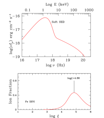
Figure 1: Top Panel: The SED corresponding to the fiducial Soft state of the outburst of a black hole of $10M_{\odot}$. The two important components of the SED, namely, the disk spectrum and the power-law have been added following the scheme described in Remillard & McClintock (2006). See Section 2.1 for the details. Bottom Panel: The Soft SED is used in C08 (version C08.00 of photoionisation code CLOUDY) to generate the ionisation fraction of FeXXVI, to show the favourable range of the ionisation parameter, for this ion to be present in the gas (see Section 2.3 for details). The peak of the distribution is marked and the corresponding $\log\xi$ value is labeled.

The SED of BHBs essentially has two components (Remillard & McClintock, 2006). (1) A thermal component which is radiated by the inner accretion disk around the black hole, and is conventionally modeled with a multi-temperature blackbody often showing a characteristic temperature ($T_{in}$) near 1 keV. (2) A non-thermal power-law component with a photon spectrum $N(E)\propto E^{-\Gamma}$ which can be radiation due to inverse-Comptonisation of photons from the disk. During different states of the outbursts the BHBs show varying degrees of contribution from the above-mentioned components. The state where the radiation from the inner accretion disk dominates and contributes more than 75% of the 2-20 keV flux is fiducially called the Soft state (Remillard & McClintock, 2006), whereas in the canonical Hard state, the contribution of the accretion disk radiation drops below 20% in the 2-20 keV flux.

The sum of local blackbodies emitted at different radii, can be used to model the radiation from a thin accretion disk. The temperature $T_{in}$ of the innermost annulus (with radius $r_{in}$) of the accretion disk is proportional to $\left[\dot{m}_{obs}/(M_{BH}r_{in}^{3})\right]^{1/4}$ (Peterson, 1997; Frank, King & Raine, 2002), where

$$\dot{m}_{obs}=L_{rad}/L_{Edd},$$ (1)

$L_{rad}$ being the luminosity in the energy range 0.2 to 20 keV and $L_{Edd}$ being the Eddington luminosity. The package XSPEC (Arnaud, 1996) includes a standard model for emission from a thin accretion disk, called $diskbb$ (Mitsuda et al., 1984; Makishima et al., 1987). $Diskbb$ in version 11.3 of XSPEC is used to generate the disk spectrum $f_{disk}(\nu)$ - with inputs $T_{in}$ and the normalization which is proportional to $r_{in}^{2}$. A hard power-law with a high energy cut-off (at 100 keV) is added to $f_{disk}(\nu)$ to yield the full SED -

$$f(\nu)=f_{disk}(\nu)+[A_{pl}\nu^{-\alpha}\times\exp{{}^{-\frac{\nu}{\nu_{max}}}}]\times f\times\exp{{}^{-\frac{\nu_{min}}{\nu}}}.$$ (2)

The parameters for the fiducial SED to represent the Soft accretion state of a black hole of $10M_{\odot}$ (Figure 1 top panel) are chosen according to the prescription given in Remillard & McClintock (2006). We carefully selected the input parameters to closely match the SED that they used as a standard for soft state SED - that of the March 24, 1997 outburst of GROJ1655-40. In the Soft state the accretion disk extends all the way to $r_{in}=3R_{s}=6r_{G}$. The photon index of the power-law is $\Gamma=2.5$ and $A_{pl}$ in Equation 2 is adjusted so that the disk contributes 80% of the 2-20 keV flux. $\nu_{max}$ = 500 keV. For a $10M_{\odot}$ black hole, $L_{Edd}=1.23\times 10^{39}\rm{erg\,s^{-1}}$. The disk accretion is chosen in such a way that $T_{in}=0.56\,{\rm keV}$ and our fiducial Soft state SED corresponds to $\dot{m}_{obs}=0.14$, which we round off to 0.1 for the rest of the paper. Note that two additional factors - a fudge factor $f$ and an exponential lower energy cut-off $\nu_{min}$ are used to ensure that the powerlaw does not blow up at low frequencies. First, $\nu_{min}=20$ eV (and not higher) was chosen to ensure that the powerlaw had 100% flux at 2 keV, because we wanted to leave the 2-20 keV part of the power-law unadulterated, since this energy range is used to determine $A_{pl}$. Then an additional fudge factor $1/1.01$ was needed to ensure that below 2 keV the power-law will never be more than 10% of the diskbb flux.

2.2 The MHD Solutions

In Paper I we had thoroughly investigated “cold” (described in F97) and “warm” (described in Casse & Ferreira, 2000b; Ferreira, 2004) MHD solutions to check if they form feasible models to explain observable winds in BHBs - winds that can be detected via absorption lines of (at least) the FeXXVI and FeXXV ions. While the details of those investigations can be checked out from Paper I and references therein, we mention some of the salient points of the MHD solutions, here, in this section.

We use MHD solutions that describe steady-state, axi-symmetric outflows, from the turbulent disk mid-plane to the ideal MHD jet asymptotic regime. The main assumptions are:
(1) The existence of a large-scale magnetic field of bipolar topology threading the whole accretion disk. The strength of the required vertical magnetic field component is obtained as a result of the solution (Ferreira & Pelletier, 1995, F97).
(2) The disk is fully turbulent, which leads to enhanced (anomalous) transport coefficients, such as viscosity and magnetic diffusivities allowing the plasma to diffuse through the field lines inside the disk. As turbulence is expected to be active only within the disk, the vertical profiles of these coefficients were assumed to decrease on a disk scale height.

The rigorous mathematical details of how the isothermal MHD solutions for the accretion disk outflow are obtained are given in the above-mentioned papers and summarized in Paper I. Hence, we refrain from repeating them here. In Paper I we found that the radial exponent, $p$ (referred hereafter as ejection index) in the relation $\dot{M}_{acc}\propto r^{p}$ (labeled $\xi$ in F97, Ferreira et al., 2006; Petrucci et al., 2010, etc.) is a key parameter that affect the density $n^{+}$ [or $\rho^{+}$ (see Equation 3)] of the outflowing material at a given radius $r$ in the disk.

The larger the exponent $p$, the more massive and slower is the outflow. The wind density is a crucial quantity when studying absorption features. For a disk accretion rate $\dot{M}_{acc}(r)$ at a given cylindrical radius $r$, the corresponding wind density at the disk surface scales as

$$n^{+}=\frac{\rho^{+}}{m_{p}} \propto \frac{p}{\varepsilon}\frac{\dot{M}_{acc}}{4\pi m_{p}V_{K}r^{2}}$$ (3)

where $m_{p}$ is the proton mass and the superscript ”+” stands for the height where the flow velocity becomes sonic. Here, $V_{K}=\Omega_{K}r=\sqrt{GM_{BH}/r}$ ($G$: gravitational constant) is the Keplerian speed and $\varepsilon=\frac{h}{r}$ is the disk aspect ratio, where $h(r)$ is the vertical scale height at the radius $r$. In Paper I, our detailed analysis showed that for the detectable wind, the ejection index $p$ plays a much more definitive role in determining the physical parameters of the wind than $\varepsilon$. Hence, for the rest of this paper, we hold $\varepsilon=0.01$ and study the resulting physical properties and spectrum for variations of $p$.

The asymptotic speed of the magnetically-driven wind $u_{\infty}$, flowing along a magnetic surface anchored at a radius $r$, can reach a quite large value. Indeed $u_{\infty}=V_{K}\sqrt{2\lambda-3}$, where $\lambda\simeq 1+\frac{1}{2p}$ is the magnetic lever arm parameter (F97), so the smaller $p$ and the faster the wind. However, as shown in Paper I, wind signatures are emitted from the densest regions right above the disk, where the flow velocity is still very low.

We point the readers to note that both the density at the base of the flow and the geometry of the matter stream lines in the flow are intrinsically related to the disk parameters. So whenever such models will be used for fitting observed data in the future, one would always have constraints on some of the disk parameters.

In Paper I, we studied two classes of MHD solutions - ”cold” and ”warm”. The outflow is termed ”cold” when its enthalpy is negligible when compared to the magnetic energy, which is always verified in near Keplerian accretion disks. The cold MHD solutions cannot achieve high values of $p\gtrsim 0.1$, when the magnetic surfaces are isothermal (F97) or even when the magnetic surfaces are changed to be adiabatic (Casse & Ferreira, 2000a). On the other hand, if some additional heat is deposited at the disk surface layers (through illumination for instance, or enhanced turbulent dissipation at the base of the corona), it is possible to get warm MHD solutions which can attain larger values of $p\lesssim 0.45$. The reason for emphasis on larger values of $p$ is because, in Paper I we found clear indication that a large value of $p>0.1$ is needed to have the physical parameters of the wind consistent with observations. Cold MHD solutions have been therefore ruled out as models for winds in accretion disks around BHBs.

Even while considering just the warm solutions, in Paper I we were limited to solutions with $p\leq 0.11$. In order to better explore the effect of the disk ejection efficiency $p$, we played also with the turbulence parameters, allowing to obtain two additional warm solutions with $p=0.30$ and $0.45$. In Appendix Section A, we have presented a brief description on the physics of obtaining these denser warm MHD solutions.

2.3 Constraints from atomic physics

The MHD solutions that were described in details in Paper I, can be used to predict the presence of outflowing material over a wide range of distances because of the self-similarity criterion - the associated equations can be found as Equations 5 - 8 of Paper I. As a result, the outflowing material, in each of these solutions, spans wide ranges in all the physical parameters like, ionization parameter, density, column density, velocity, and timescales. However, only part of this outflow can be detected through absorption lines; we refer to this part as the “detectable wind”. Literature survey of BHB high resolution spectra shows that commonly absorption lines from H- and He-like Fe ions are detected (e.g. Lee et al. 2002, Neilsen & Lee 2009, Miller et al. 2004, Miller et al. 2006, and King et al. 2012). Further, Ponti et al. (2012) made a very important compilation of detected winds in BHBs, also concentrating their discussion around the line from FeXXVI. Hence, we choose the presence of the ion FeXXVI as a proxy for “detectable winds”.

It is the ionization parameter, which is the key physical parameter to determine the region of the “detectable wind”, because the observable tracers, in this case, are absorption lines from different ionic species. Since the absorption lines in question (mainly from FeXXVI and FeXXV) manifest themselves in X-rays, we use the definition most commonly used by X-ray high resolution spectroscopists, namely $\xi=L_{ion}/(n_{H}r^{2}_{sph})$ (Tarter et al., 1969), where $L_{ion}$ is the luminosity of the ionizing light in the energy range 1 - 1000 Rydberg (1 Rydberg = 13.6 eV) and $n_{H}$ is the density of the gas located at a distance of $r_{sph}$. There is a simplifying assumption that gas at any given point within the flow, is illuminated by light from a central point source. This approach is not a problem unless the wind is located at distances very close to the black hole ($\leq 100r_{G}$). As we have seen in Paper I that the ”detectable wind” is much further out (also see Figure 4), we can continue with this reasonable assumption. The SED for this ionising radiation is the same as discussed above, in Section 2.1.

Ion fraction (IF) $I(X^{+i})$ of the $X^{+i}$ ion measures the probability of its presence.

$$I(X^{+i})=\frac{N(X^{+i})}{f(X)\,N_{\rm{H}}}$$

gives the fraction of the total number of atoms of the element $X$ that are in the $i^{\rm{th}}$ state of ionization; where $N(X^{+i})$ is the column density of the $X^{+i}$ ion and $f(X)=n(X)/n_{\rm{H}}$ is the ratio of the number density of the element $X$ to that of hydrogen. The bottom panel of Figure 1 shows the ion fraction of FeXXVI calculated using version C08.00 of CLOUDY (Ferland et al., 1998, ; hereafter C08) for Solar metallicity (Allende Prieto et al., 2001, 2002) gas that is illuminated by the Soft state SED. The ion fraction is seen to peak at $\log\xi=4.86$. However, note that even at $\log\xi=6.0$, the ion fraction is 0.1, i.e. 10% of iron is in FeXXVI. Thus, $\log\xi_{max}|_{FeXXVI}=6.0$ - the conservative upper limit beyond which the ion fraction for FeXXVI drops below 10%. We shall use this limit of $\log\xi_{max}=6.0$ to constrain our MHD solutions, throughout this paper (unless otherwise mentioned).

2.4 Constraining the MHD solution to find the “detectable wind”

For locating the “detectable wind” region within the MHD outflows, we impose the following physical constraints to remain consistent with the various observational criterion mentioned in the previous sections:

• In order to be defined as an outflow, the material needs to have positive velocity along the vertical axis ($z_{cyl}$);

• To ensure a wind which is not Compton thick we impose that the integrated column density along the line-of-sight satisfies $N_{H}<10^{24.18}{\rm{cm^{-2}}}$. Through this we get an idea about how close to the accretion disk can we probe through the absorption lines.

• We impose that $\xi\leq 10^{6}\,\,{\rm{erg\,cm}}$ (where FeXXVI has IF $\gtrsim 0.1$) for the Soft state, because over-ionized gas cannot cause any absorption and hence cannot be detected.

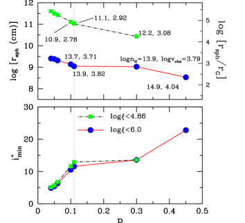
Figure 2: Physical parameters for the IP of the wind region detectable through FeXXVI absorption lines. The vertical dotted line shows the extent of $p$ that was used in Paper I. Further, in both the panels, the constraint of $\log\xi_{max}|_{FeXXVI}$ are evident by the use of two different legends. The dotted and dashed, black lines interspersed with the green squares, shows the more stringent cut-off $\log\xi_{max}|_{FeXXVI}=4.86$ used in Paper I. In the current paper we use $\log\xi_{max}|_{FeXXVI}=6.0$, whose results are indicated by the solid, red lines interspersed by the blue circles. Top Panel: It shows how far the absorber is from the central black hole. This is the minimum distance derived from $\log\xi_{max}|_{FeXXVI}$ (= 6.0 or 4.86). The two numbers placed close to some of the points indicate the corresponding values of log$n_{H}$ and log$v_{obs}$ of the wind at this minimum distance. Bottom Panel: The lowest line-of-sight along which we can expect to probe the gas, derived from the condition of $N_{H}<10^{24.18}{\rm{cm^{-2}}}$.

Following conditions 1 and 2, we can find the $\sim$ lowest line-of-sight along which we can probe the gas - expressed as $i_{min}$ in the bottom panel of Figure 2. Then we impose condition 3 to ensure the presence of the ion of our interest (in this case FeXXVI). Using the last condition, we can thus find the closest point “Innermost Point” (hereafter IP) to the black hole which satisfies these conditions. As said at the end of the previous section, this point will have a ionisation parameter $\log\xi_{max}|_{FeXXVI}\sim 6.0$. However, for different MHD solutions, these IPs (shown using solid, red lines interspersed by the blue circles in Figure 2) will be at different distances from the black hole, and will also have different values of density and velocity, although all of them will have near constant ionisation parameter $\log\xi_{max}|_{FeXXVI}\sim 6.0$. The Top Panel of Figure 2 gives us a quantitative comparison of the physical parameters of the IP of the various warm MHD solutions. A careful consideration of this comparison aids us in choosing the MHD outflow models for further investigation. Further note that, in Paper 1, we had used a more stringent constraint on $\log\xi_{max}|_{FeXXVI}\,\,(=4.86)$. In Figure 2, we have also shown the position (and physical parameters) of the resultant (Paper I) IPs using a different legend - dotted and dashed, black lines interspersed with the green squares.

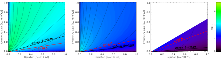
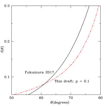
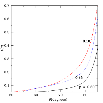
Figure 3: Top panels: The spacial distribution of the MHD solutions is shown - p = 0.10 (left panel), p = 0.30 (middle panel) and p = 0.45 (right panel). The colour gradient shows the distribution of the ionisation parameter (in logarithmic scale). The thin, solid, black lines are the streamlines through which matter flows out following the magnetic field lines. The thick, solid, black line indicates the position of the Alfven surface for each of the solutions. The solid, red line shows the minimum line-of-sight angle (from the mid-plane of the accretion disk) above which it is possible to detect the wind through absorption lines of FeXXVI. The values of these angles are marked close to this line of sight. Bottom panels: We show a comparison of the density functions, which is the variation of the density against $\theta(=90^{\circ})-i$, i.e. the variation of density along the stream line. Comparison of our $p=0.1$ MHD model with the one that was used by Fukumura et al. (2017) is presented in the left panel and on the right panel, we show the comparison among the three MHD models that are used in this paper.

The density reported for most of the observed BHB winds $\geq 10^{11}\,\rm{cm^{-3}}$ and the distance estimates place the winds at $\leq 10^{10}\,\rm{cm}$ (Schulz & Brandt, 2002; Ueda et al., 2004; Kubota et al., 2007; Miller et al., 2008; Kallman et al., 2009). Our analysis in Paper I had shown that the “detectable wind” part of the cold MHD outflows were too far away from the black hole and hence had lower density ($n_{H}<10^{10}\rm{cm^{-3}}$) and lower (line-of-sight) velocity ($v_{obs}<10^{2}\rm{km/s}$) than what is expected from the above mentioned observations. Cold MHD solutions were thus ruled out as viable models for disk winds in BHBs. We had further investigated the warm MHD solutions in Paper I and found that they indeed, can have higher $p$ values which are needed to have dense enough outflows, so that the IP moves closer to the black hole, so that the values of the physical parameters of the IP are consistent with the observations. In Paper I, even for the warm solutions we were limited to $p=0.11$. We realised that some observations require the wind to be closer to the black hole and thus have higher velocity and density than what the densest $p=0.11$ warm solution could predict as a model. Thus, we felt the need for denser warm MHD solutions with higher $p$ values (see Section 6.1.2 of Paper I).

Figure 2 shows comparisons among the MHD outflow models and also comparison between the constraints considered in Paper I and in this paper. Notice that the $\log\xi_{max}|_{FeXXVI}=4.86$ lines (black, dotted-and-dashed) do not extend to p = 0.45 - that is because such low ionization gas was not found within the Compton thin region of the p = 0.45 MHD outflow. In comparison, the red, solid curve joining the blue circles show the result for the ‘standard’ $\log\xi_{max}|_{FeXXVI}=6.0$ used in this paper. Although the lowest line-of-sight angle, where we can expect to detect FeXXVI absorption, does not vary much as a function of $\xi_{max}$, the distance of the IP to the BH drops by a factor of $\sim 100$ for almost all the MHD solutions tested, while the density at that point goes up by $\sim 1.5-3$ dex and velocity by $\sim 0.7-1$ dex. In Paper I, we had predicted this possibility in Section 6.1.1. The vertical black, dotted line, cutting across the panels in Figure 2 shows the other major change that has happened in our analysis, since Paper I. As mentioned above, in Paper I, we were limited to warm MHD solutions with $p\lesssim 1.1$ - the value which has been marked by the dotted line. For this paper we have been able to investigate two more solutions which are more “massive”, with p = 0.3 and 0.45. See Appendix Section A, for a brief description on the physics of obtaining these denser warm MHD solutions.

We choose to investigate the warm solutions with $p=0.1$, 0.3 and 0.45 for further understanding and for deriving spectra. The aim is to see how different the line-of-sight absorption features are, as a function of $p$, $i$ (or $\theta$) and the size of the disk.

The top three panels of Figure 3 gives a visual comparison of the three solutions. As is evident from the changing gradient of $\log\xi$ values across the three panels, as p increases, the value of $\xi$ decreases at a given $r$, because the solutions are denser with increasing $p$. The red solid line, in each of those panels, near which the value of $i$ is labeled, is the lowest line-of-sight for which the wind is not Compton thick. The wind will be detected via FeXXVI absorption lines, only from regions above the red, solid line. Notice that the smallest angle for which the wind can be detected, moves further away from the accretion disk, as $p$ increases. For $p=0.30$ and 0.45, the relevant region is also beyond the Alfven surface. In the next section, where we derive spectra, we choose representative line-of-sight close to the value (of minimum $i$) mentioned in Figure 3.

In the bottom panels, we have shown comparison between the density functions of the MHD solutions. The left panel shows a comparison between our $p=0.1$ MHD model and the outflow model used in Fukumura et al. (2017). On the right, it is the comparison of $f(\theta)$ of the three MHD models that are being studied in this paper. It is interesting to note that there is a non-monotonic behaviour of $f(\theta)$ as function of p. As mentioned before, we were motivated to find warm MHD models with higher values of $p$, as indicated necessary from Paper I. However, to obtain MHD solutions with high $p$ values one needs to change other disc parameters (namely turbulence, heating). This translates into different outflow geometries, as discussed in Section A showing that some solutions bend and open up much more than others (Figure 14). This is the reason of the non-monotonic behavior of the density function - the link between the $f(\theta)$ profile and $p$ is not straight forward.

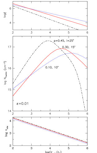
Figure 4: The three most important observables predicted from C08 simulations for our models and lines of sight. The models and the lines of sight are explicitly labeled in the middle panel which shows the distribution of the column density of the ion FeXXVI along the line of sight. The same line styles and colours are maintained in the top panel (showing distribution of ionisation parameter) and bottom panel (showing distribution of the line of sight velocity).

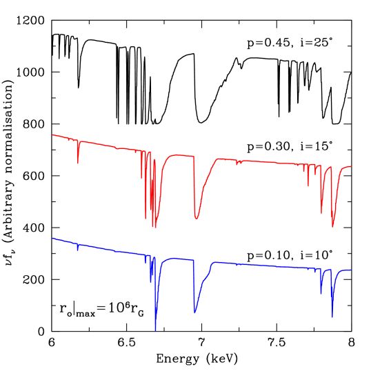
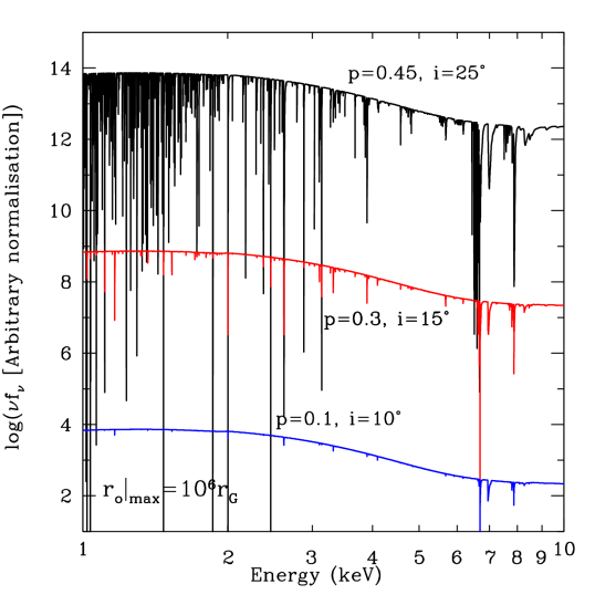
Figure 5: This Figure shows variation of spectrum as the MHD Solutions are varied. The left panel just zooms in on the 6-8 keV energy range concentrating on the FeXXV and FeXXVI line complexes. On the right panel, we show the entire energy range of 1-10 keV relevant for X-ray observations of X-ray binaries.

3 Theoretical Spectra of MHD winds using CLOUDY

The 1st step in calculating synthetic spectra using C08, is to determine the velocity or energy resolution for which we want to derive the spectra. The maximum energy resolution that C08 can provide corresponds to 75 km/s (1.6 eV) at $\sim 6.5$ keV. In comparison the projected resolution at XRISM is 300 km/s (6.4 eV) and that of Athena is  150 km/s (3.2 eV) at   6.5 keV. The average velocity resolution that Chandra provides at 1 keV is 1500 km/s (32 eV) and deteriorates for 6.5 keV. Since the resolution of the theoretical spectra should be better than that for the observed spectra, we choose to accept the best theoretical resolution possible using C08, at this stage - 75 km/s. Our theoretical velocity resolution is still better than even what Athena will provide a decade later.

For any given line-of-sight (e.g. $i=10^{\circ}$ for p=0.1) the gas is modeled as a continuous set of slabs/boxes separated by $\Delta v=75$ km/s. Thus each slab/box is a ‘small’ unit of the flow itself, and the velocity of the box is simply the flow velocity at that physical point. We find the ‘gas slab’ with log$\xi$ = 6 and start C08 calculations from that distance. The 1st box sees the light coming from the central source, but redshifted by the velocity of the 1st box, away from the source. Box 2 onwards, any box n ‘sees’ the SED transmitted to it from box n-1, but blueshifted by the velocity difference of the two boxes. For each box, we are calculating the transmission coefficients as a function of energy, which results in the absorption spectrum. In this paper, we do not include the emission lines, from any of the boxes. While calculating the absorption spectrum from each box, we are also recording the important physical parameters (some of which are plotted in Figure 4), which will help us understand the spectrum along a line of sight. Note that while analysing each box, we explicitly check that the box is not Compton thick, by checking $N_{H}<10^{24.18}\,\,\rm{cm}^{-3}$, as well as the cumulative column along the line-of-sight is $<10^{24.18}\,\,\rm{cm}^{-3}$. The calculation is continued until we reach the end of the disk, or velocity of the box drops below 75 km/s. The extent of the wind is determined by the maximum anchoring radius, which is varied as $r_{o}|_{\rm{max}}=10^{5}\,\&\,10^{6}r_{G}$ to test the effects on the spectra. We repeat these calculations for different lines of sight for the three different warm MHD solutions with p = 0.10, 0.30, 0.45.

We note that the disk extent of $10^{6}r_{G}$ for a 10 solar mass black hole is $1.5\times 10^{12}$ cm. It is on the higher side of what can be expected for disk sizes for stellar mass black holes. GRS 1915+105, the brightest galactic black hole is known to have a large disk $\sim 10^{12}$ cm (Done, Wardinski & Giellinski, 2004; Remillard & McClintock, 2006). Hence we keep our simulations till $r_{o}|_{\rm{max}}=10^{6}r_{G}$. We further checked that there is very little effect of the disk size on the spectrum or the equivalent widths, as will be mentioned in subsequent sections as well. Hence we show many of our simulations for $r_{o}|_{\rm{max}}=10^{6}r_{G}$, instead of for $10^{5}r_{G}$.

In Figure 4, we see the results of probing p=0.1 along i = 10, p=0.3 along i = 15, and p = 0.45 is probed along i=25. We can trace the column density of the FeXXVI as a function of the distance from the black hole. The figure demonstrates that for denser MHD solutions we can probe material closer to the black hole, since we get intense FeXXVI absorption closer to the black hole. Also, note that closer to the black hole means higher velocities. Hence for denser solutions we have intense FeXXVI absorption lines which are further blueshifted. However, along a line-of-sight since there is ‘continuous’ absorption over a range of $\xi$, the resultant absorption will be an amalgamation of many absorption lines/components spread over a range of $\xi$ and $v$. The lines will be more skewed for the denser MHD solutions, because of this reason. We will see this effect in Figures 5 and 6.

Figure 5 shows how the spectrum changes when we consider different MHD solutions. The denser solutions with higher value of p have more skewed and deeper lines (left panel). Notice that the denser solutions also show ”satellite lines”. Lines that come from lower ions of iron (Kallman, 2004; Witthoeft, 2011). The requirement for these lines is that they need low ionisation (much lower than FeXXV). The 1-10 kev spectra of the same models show that absorption lines of sufficient strength can be observed from low ionisation ions (corresponding to elements with lower atomic number) for the denser (higher $p$) MHD models.

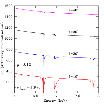
Figure 6: This Figure shows variation of spectrum as the line-of-sight angle is varied for the p=0.1 MHD solution.

We also generated spectra for different wind extent, while keeping $p$ and $i(\theta)$ constant. A larger wind extent (for a given solution) will come from extending the disk further so that the last anchoring radius can be further out from the black hole. The effect of a larger size of the accretion disk is similar as having a denser (higher $p$) MHD model, in one way - we can have wind further out from the black hole. As a result the ionisation of the gas which is furthest out will be lower. Hence effects of lower ionisation will show up for larger disk. However, we found one distinction from the case of the denser MHD models as well. The lower $\xi$ ions for the larger disks have lower velocity (and hence narrower line profiles or lesser skewness) than those for denser MHD solutions.

Figure 6 shows the variation of spectrum as the angle of line-of-sight changes. As we go up from the accretion disk (i increases, $\theta$ decreases), the line strengths decrease. Here we show only the case of p=0.1 where the effect is the most noticeable compared to larger $p$ values. The p = 0.1 model has a sharper gradient (fall of density with decreasing LOS angle $\theta$) at $\theta=80^{\circ}(i=10^{\circ})$ than what p = 0.3 has at $\theta=75^{\circ}(i=15^{\circ})$ or p = 0.45 has at $\theta\sim 65^{\circ}(i\sim 25^{\circ})$. Hence, as $\theta$ decreases (and i increases), the p = 0.10 solution changes more significantly and hence the lines change significantly.

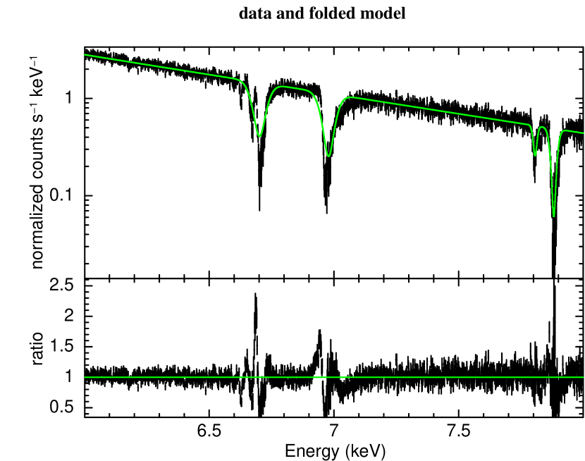
Figure 7: Athena simulation of a spectrum corresponding to a MHD disk wind with an ejection efficiency $p=0.30$, a radial extension of 10${}^{6}r_{G}$ observed along an inclination angle of $15^{\circ}$. The source has a flux of 100 mCrab and the simulation has a 100ks exposure. This corresponds to a total number of counts of 240$\times 10^{3}$ in the 6-8 keV energy range. The spectrum has been re-binned in order to have at least 10 counts per bin. Top: the solid, green line show the best fit model which combines two power laws for the continuum and 4 Gaussian absorption lines at fixed energies 6.7, 6.96, 7.8 and 7.88 keV. Bottom: Ratio data/model.

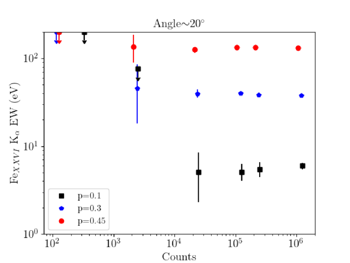
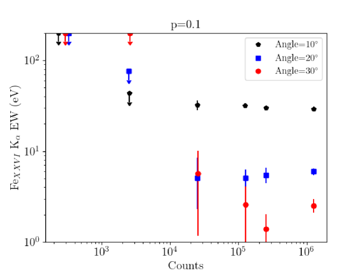
Figure 8: EW of the Fe XXVI line versus the total number of counts in the 6-8 keV range. The simulations correspond to a wind extension of $10^{6}r_{G}$. Left: We look for the effect of varying the ejection index $p$ at same or similar inclination angles. Models with $p=0.1$ (black-square) and $p=0.3$ (blue-pentagon) were studied at line-of-sight angle $i=20^{\circ}\,\,(\theta=70^{\circ})$, whereas the $p=0.45$ (red-circle) model was examined at $i=23^{\circ}$ (because it is optically thick below this angle). Right: We study the effect of varying inclination angle for a fixed ($p=0.1$) MHD model. The black-pentagon, blue-square and red-circle points respectively correspond to inclination angle of $i=$ 10, 20 and 30 degrees ($\theta$ = 80, 70 and 60 degrees).

This section shows us clearly that there are variations in the theoretical spectra, and the line shapes, as the MHD flow parameters are changed, or when we view the flow through different inclination angles. However, this analysis is not sufficient to tell us if these theoretically apparent variations are large enough to be distinguished in observations. Hence we dedicate the whole next section trying to answer that question.

4 Athena and Xrism Spectra of BHB winds

4.1 Basics of simulating XIFU and XRISM synthetic spectra

We simulated observations for the high resolution instruments on two planned future X-ray missions, the Resolve spectrometer on the X-ray Imaging and Spectroscopy Mission (XRISM; Makoto et al., 2018) and the X-ray Integral Field Unit (X-IFU) on Athena (Barret et al., 2018). Simulations for Resolve, were made based on response matrices, effective area curves, and backgrounds for the Hitomi Soft X-ray Spectrometer (Leutenegger et al., 2018) which were provided by NASA-GSFC (https://heasarc.gsfc.nasa.gov/docs/xrism/proposals/). For Athena, we used the X-IFU simulation pipeline xifupipeline, which is part of end-to-end simulation package SIXTE (Dauser et al., 2019). The simulation employed here includes the official effective area of Athena’s telescopes with an effective area of $1.4\,\mathrm{m}^{2}$. For bright source simulations, xifupipeline includes a model for the degradation of the energy resolution of the micro-calorimeter array that happens when photons hit the same pixel close in time to each other. For the brightest assumed source fluxes, we also performed simulations where a Be-filter with a thickness of $100\,\mu$m is put in front of the detector array. This approach cuts the flux of the soft X-rays and allows X-IFU to perform observations even of bright sources.

4.2 Single Gaussian Fits to the fake spectra

4.2.1 General methodology

We develop an automatic procedure to test the presence of absorption lines in the simulated spectra. For most of the analysis, we concentrate on the 6-8 keV range where the most predominant absorption lines reside, especially from Fe XXV and Fe XXVI. We first fit the continuum with two power laws (to reproduce any potential curvature in the continuum), ignoring data between 6.5 and 7.2 keV and above 7.7 keV. Then we add, one by one, 4 Gaussian lines in absorption centred at 6.7, 6.96, 7.8 and 7.88 keV. These energies correspond to FeXXV (1s²-1s2p), FeXXVI (1s-2p), NiXXVII (1s²-1s2p) and FeXXV (1s² -1s3p) respectively. For each Gaussian, the energy was fixed but their width, redshift (z) and normalisation were left free to vary.

An example of best fit obtained through this procedure is shown at the top of Figure 7, while the ratio data/model is shown at the bottom. This is an Athena simulation of a spectrum corresponding to a MHD disk wind with an ejection efficiency $p=0.30$, a radial extension of 10${}^{6}r_{G}$ observed along an inclination angle of $i=15$deg ($\theta=75$deg). The source has a flux of 100 mCrab and the simulation has a 100ks exposure. This gives a total number of counts in the 6-8 keV range of about 240$\times 10^{3}$. We clearly see the presence of absorption features around 6.7, 7, 7.8 and 7.9 keV.

The procedure correctly finds these four main absorption features but clear residuals are present around each line - indicating that the line has a more complex profile than a simple Gaussian one. We also see small absorption features to the left of the FeXXV line at $\sim$6.7 keV, which are the ’satellite lines’ either from the lower ions of iron, or the x, y, z resonance lines of the FeXXV ion. This simpler method is used in the immediate next subsections to get an idea of - i) the number of counts needed to detect the lines; ii) the detectability of the line asymmetries as the ejection index, and LOS angle vary; and iii) to study Athena spectra in the 1 - 10 keV energy range. The single Gaussian fits clearly demonstrate the need to fit the absorption lines with more complex profiles or multiple Gaussians. The latter is attempted in Section 4.3.

4.2.2 Minimum counts needed

We have reported in Figure 8 the EW of the Fe XXVI K$\alpha$ line, deduced from our fitting procedure, versus the total counts in the 6-8 keV range for different sets of parameters. This figure corresponds to the case of a wind radial extension of $10^{6}r_{G}$. On the left of Figure 8, the inclination is chosen to be $~{}20^{\circ}$ and the wind simulations have different p=0.1, 0.3 and 0.45 for the black squares, blue diamonds and red circles respectively. On the right of Figure 8, the ejection parameter p is fixed to 0.1 and the wind simulations have different inclination angle of 80, 70 and 60 degrees for the blue diamonds, black squares and red circles respectively. As expected, the absorption lines are stronger (the EW are larger) for larger ejection parameter p and larger inclination angles.

Interestingly, this figure gives an estimate of the required number of counts, and consequently the required combination of source flux and exposure, so that the Fe XXVI K$\alpha$ line can be detected. The counts in the 6-8 keV band has to be larger than a few thousands to allow good detection. Lines with EW as low as a few eV should be detectable if the 6-8 keV counts is larger than $10^{4}$-$10^{5}$ for the less favourable simulated cases i.e. low p (=0.1) and higher inclination angles in terms of i (lower inclination angle in terms of $\theta$).

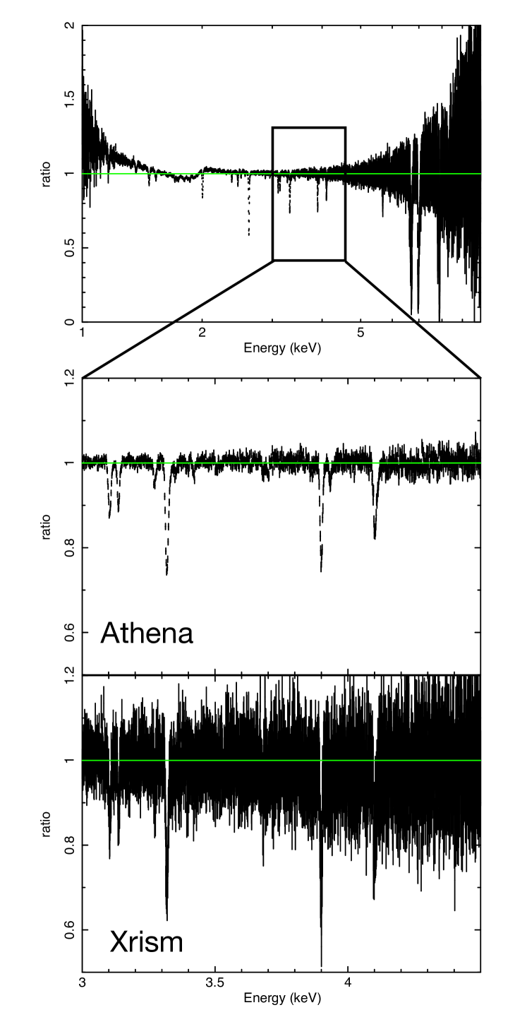
Figure 9: Top: 1-10 keV simulated spectra with Athena assuming $p=0.3$, an angle $i=15$deg and a disk extension of $10^{6}r_{G}$. The source has a flux of 100 mCrab and the exposure was 100 ks. Middle: A zoom of the 3-4.5 keV energy range. Absorption lines of Ar and Ca are clearly visible. Bottom: Same simulation but with XRISM. The spectra have been re-binned in order to have 15$\sigma$ per bin.

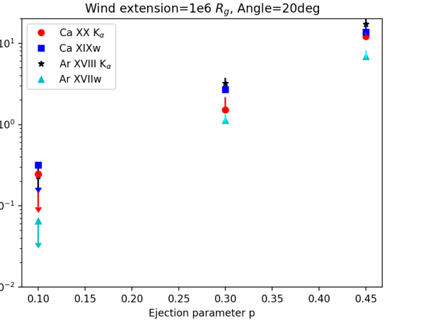
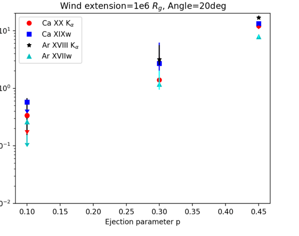
Figure 10: EW of ArXVIII and CaXX lines for MHD solutions with different ejection indices - p = 0.1, 0.3, 0.45, but of same disk extent $r_{o}|_{max}=10^{6}r_{G}$. The left plot is for Athena simulations and the right one for XRISM. For the simulations we assume a source flux of 100 mCrab and an exposure of 100 ks

4.2.3 Athena spectra variation with $p$ and $i$

Complementary to the analysis in Section 3, we conducted Athena simulations (still assuming a source of 100 mCrab flux in 2-10 keV and observed for 100 ks) for spectra which vary with ejection index $p$ and LOS angle $i$. For the details and Figures we urge the reader to check Section C, in the Appendix. Here, we summarise our finds, based primarily, on the FeXXVI K$\alpha$ absorption line.

As expected the absorption lines are stronger for larger ejection efficiency parameter $p$. We found that it is not possible to detect the asymmetry in the line profile for p = 0.1, even if it can be seen in the theoretical spectra. Like the strength of the lines, the asymmetry also grows as p increases (0.3 or higher). Even the single Gaussian fit (even if inaccurate) captures the fact that the absorption line profile peaks at higher energy (stronger blueshift) for higher $p$.

Since, we could not detect line asymmetry for $p=0.1$, we chose the $p=0.3$ MHD solution for studying the variation of Athena spectra as LOS angle changes. Since we chose a higher $p$ solution, the line remains detectable even viewed at large inclination from the disk surface - $i=40^{\circ}=(\theta=50^{\circ})$. The closer the LOS to the disk (i.e. the smaller the LOS inclination) stronger the absorption line and more asymmetric the line profile. This is expected because the wind density increases when approaching the disk surface. Beyond $i=30^{\circ}=(\theta=60^{\circ})$, line asymmetry cannot be detected. Here we do not see any significant shift in the blueshift of the Gaussian fit line, as was the case for $p$ variation.

4.2.4 The 1-10 keV spectrum

In the right panel of Figure 5 we have seen theoretical spectra harbouring absorption lines at energies less that 6 keV. We need to check if these lines can be detected by Athena and XRISM. It would be interesting to check if in observed spectra we can trace the change in the line observable as the MHD flow changes. These lines were not strong enough or asymmetric enough to warrant multiple Gaussian fits. Hence, single Gaussian fits have been used to calculate EWs.

We have reported in Figure 9 the 1-10 keV simulated spectra expected with Athena and XRISM with $p=0.3$, an angle $i=15^{\circ}$ and a disk extension of $10^{6}r_{G}$. Lines are observed in the entire 1-10 keV range and we clearly see Argon and Calcium lines in Athena and, while less significantly, also in XRISM.

We have discussed in Section 3 that having a higher $p$ dense MHD model and/or having a larger extent of the accretion disk increases the chances of ‘seeing’ the absorption lines from the H and He-like ions of lower atomic number elements like Argon and Calcium. Through the simulations for Athena and XRISM we can verify the above quantitatively. In Figure 10 we show the EW of ArXVIII and CaXX lines for ATHENA (left panel) and XRISM (right panel). The variation of the EW is with respect to changing MHD models (p = 0.1, 0.3 at LOS $i=20^{\circ}$ and p =0.45 at LOS $i=23^{\circ}$), while the disk is assumed to have a constant extent of $r_{o}|_{max}=10^{6}r_{G}$. We had also tried changing the disk extent from $r_{o}|_{max}=10^{5}$ to $10^{6}r_{G}$ (not shown in the Figure), while keeping the MHD solution parameters constant at p = 0.3, $i=15^{\circ}$.

We found that changing the MHD model has a greater impact on the presence and strength of the absorption lines from Ar and Ca, than extending the accretion disk further out. While the disk was extended from $r_{o}|_{max}=10^{5}$ to $10^{6}r_{G}$, the EWs of the lines changed only by a factor of a few. However, as $p$ increases from 0.1 through 0.3 to 0.45 the EW change by $\sim 2$ dex.

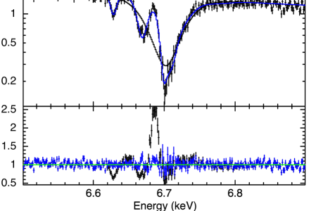
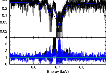
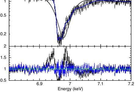
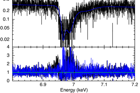
Figure 11: Left: Zoom of the Athena simulation of Figure 7 around the FeXXV (top) and FeXXVI (bottom) lines. The black line and black residuals correspond to best fits with a single Gaussian. The blue line and blue residuals correspond to best fits with a multiple-Gaussian model. In these examples, 3 Gaussians have been used to fit the FeXXV line + 3 other Gaussians to fit the absorption features below 6.68 keV, and 5 Gaussians to fit the FeXXVI line. Right: The same but for XRISM simulations. We need 2 Gaussians to fit the FeXXV line and 3 more Gaussians to fit the satellite lines at $\sim$6.63 and 6.7 keV. And we need 3 Gaussians to fit the FeXXVI line

4.3 Multiple Gaussian fits to the asymmetric absorption lines

In most cases, a fit of the absorption lines with a single Gaussian showed clear residuals around the lines as exemplified in Section 4.2. The reasons are two-fold. First, the expected line profiles are clearly asymmetric and this asymmetry becomes detectable when the statistics is good enough. On the other hand, the presence of other weak absorption lines, close to the FeXXV ones especially, ”pollutes” the fit. This is shown in Figure 11 where we plot zooms around the energy range of the FeXXV and FeXXVI lines. The black lines represent the fit obtained with a single Gaussian profile and the corresponding data/model ratio are reported in black at the bottom of each figures. The blue lines (and the corresponding blue data/model ratio) have been obtained with a multiple-Gaussians model. There is a clear improvement of the residuals when we use several Gaussians to fit the main absorption profile. We find that 3 (resp. 5) Gaussians give a statistically good fit in the case of FeXXV (resp. FeXXVI) and the addition of another Gaussian has an F-test probability smaller than 90%. We also need to add other Gaussians to fit the weak absorption features in the red part of the FeXXV line.

The XRISM simulations shown in Figure 11 have been obtained for a 100 mCrab source at line-of-sight angle $i=15^{\circ}$ observed for 100ks. The MHD model used was the p = 0.3 outflow extending up to $\rm{r_{o}|_{max}}=10^{6}r_{G}$. The fake fit needed 2 Gaussians to fit the FeXXV line and 3 more Gaussians to fit the satellite lines at $\sim$6.63 and 6.7 keV. And we need 3 Gaussians to fit the FeXXVI line

In this paper we limit ourselves to just demonstrating the power of Athena and Xrism to detect the asymmetry in the absorption lines. Of course rigorous quantitative analysis of these fits are warranted, so that more accurate measures of the EW can be prescribed. However such analysis is beyond the scope of the current paper. We intend to dedicate a separate publication, in near future, which will explicitly deal with this analysis.

5 Discussion

5.1 Comparison with Chandra

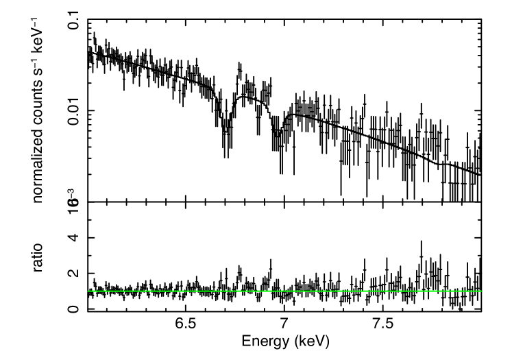
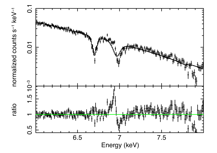
Figure 12: Simulated spectra for Chandra: for MHD model with $p=0.30$, the disk extending to $10^{6}$ observed at LOS $i=15^{\circ}$. The central source is assumed to be at 100 mCrab. The exposure times for the fake observations are chosen to be 100 ks (top) and 1 Ms (bottom)

.

We show in Figure 12 the simulation of p = 0.30, i = 15^∘, $r_{o}|_{max}$ = $10^{6}r_{G}$ MHD solution for a source of 100 mCrab observed by Chandra for 100 ks (top panel) and 1 Ms (bottom panel). The lines, of $\sim 30-50$ eV each, are clearly detected at more than 99.99% confidence already with 100 ks but the asymmetry is not. In 1 Ms however we clearly detect the asymmetry at least for the Fe XXVI line. Given the variability of XrB in outburst, in flux and in spectral shape, this 1Ms ( 11 days) Chandra observation is of course not a realistic case. It rather shows that we have to rely on the future missions like XRISM and Athena to bring such studies within practical reach.

5.2 The FeXXVI K$\alpha$ doublet lines

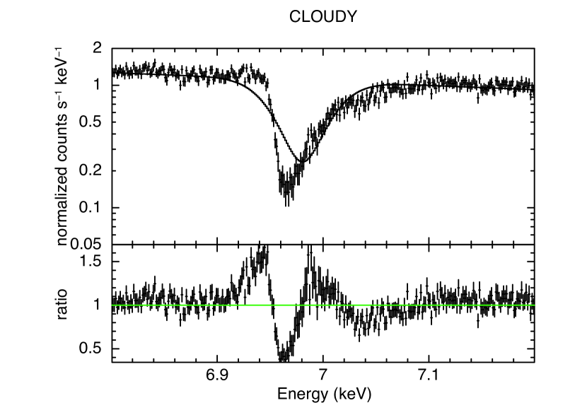
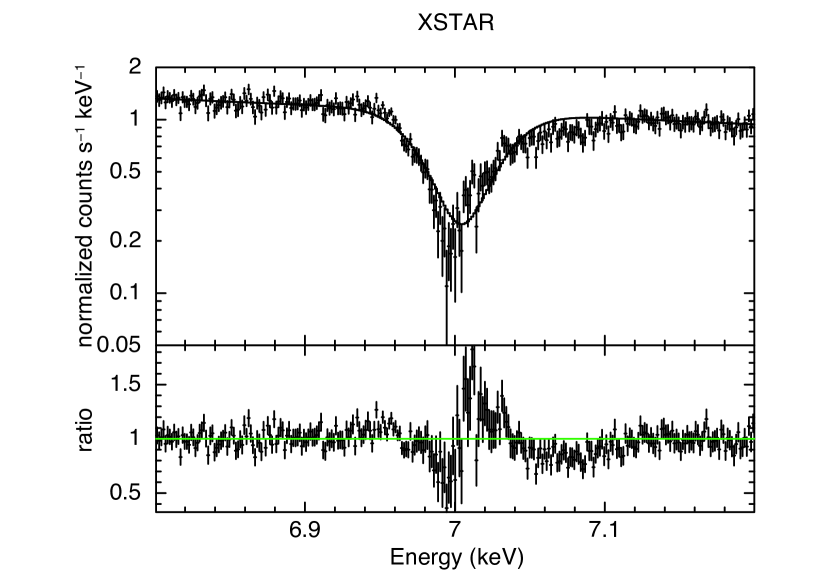
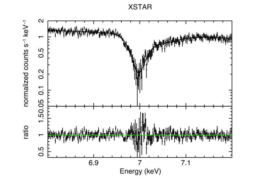
Figure 13: Top Left: Xstar simulations of the FeXXVI K$\alpha$ absorption line, highlighting the doublet feature of the line. Top Right: C08 simulation of the Fe XXVI line for $p=0.30$, $i=15$, disk extension $10^{6}$ and 100 mCrab for 100ks. The line is a best fit with a simple Gaussian line with energy fixed to 6.96 keV. Bottom Left: Same simulation than the top one but using Xstar. The FeXXVI K$\alpha$ doublet is now included. Bottom Right: Fit of the XSTAR simulation using two Gaussians at energy fixed to 6.952 and 6.973 keV.

In nature, the Lyman $\alpha$ line from the H-like ions of any element is actually split into a doublet. For iron, they are Fe XXVI Ly$\alpha_{1}$ at 6.973 keV and Fe XXVI Ly$\alpha_{2}$ at 6.952 keV. It is very difficult to detect these two lines distinctly even in a Chandra-HETG spectrum, which has the best energy spectral resolution available, among current X-ray observatories. Tomaru et al. (2020) have analysed the Chandra HETG 3rd order spectrum of neutron star low mass X-ray binary GX 13+1 and model these two lines. They have discussed in details the importance of these lines in the upcoming era of X-ray astronomy. Upcoming observatories like XRISM (and subsequently Athena) with significantly improved energy spectral resolution will be able to ‘easily’ find the doublet. Analysing the shape of the lines will shed light on the launching and acceleration mechanisms of the outflowing wind.

The C08 atomic data base records the Fe XXVI Ly$\alpha$ as a single line - a blend of the doublets. It is not a problem for most current observations, because these features can hardly be observed as separate lines. All our above analysis is based on this blended line. To consider the details of the doublets is beyond the scope of this paper, however in this section we show some preliminary results of how the doublet may be seen by Athena. For the analysis in this section, we had to use XSTAR.

In top left panel of Figure 13 we show the zoom of the Fe XXVI Ly$\alpha$ line region. Three different warm MHD models have been considered. As $p$ increases the doublets get smeared out. We use the $p=0.3$ model and its spectrum to further do Athena spectrum (bottom panels of Figure 13). The top right panel of Figure 13 show Athena simulations derived out of the C08 calculations. The Fe XXVI Ly$\alpha$ line in the Athena fake data is fit with a single Gaussian with line energy fixed at 6.96 keV. Notice that significant residuals remain. When the same analysis is done, but this time using the XSTAR generated spectrum (bottom left panel of Figure 13), the residuals improve. However, if instead of one Gaussian, if two are used with line centres placed at the natural energies of the doublets, the fit leaves almost no residuals (bottom right panel of Figure 13) - clearly indicating that Athena spectrum can constrain the doublets.

Further detailed quantitative analysis is beyond the scope of this paper. Because in this paper we are dealing with ‘denser’ MHD models, the doublets from such flows are more smeared out. However in future publications we will deal with lower density MHD models and look for their observable signatures. It would be more relevant at that stage to look into further details of the doublet lines and their variations (with the MHD models), and also check the potential of the lines as a deterministic observable.

5.3 Comparison with past literature

While there is a significant amount of literature on theoretical development of MHD outflow models and also their application to Jets’ observations, there is only a limited number of attempts in applying MHD models as explanations for the observed lower velocity ($\sim 100$ km/s) diffused winds. Fukumura et al. (2010a, b, 2014) is where they were first attempted for explaining the various wind components in super-massive black hole systems or the Active Galactic Nuclei. Fukumura et al. (2017, 2021) show extensions of the same models and their methods to explain winds in Black hole X-ray binaries.

First paper Fukumura et al. (2010a) gives us the framework of the models and shows different outflow models, mainly varying $\theta$ (the inclination angle), while holding the other parameters (namely $\eta_{w}$ and $\dot{m}$) constant (see Eqns. 28 and 29 of the paper). The calculations of the paper were done keeping AGN absorbers in mind, however the paper acknowledges that the same models are scalable to different black hole masses. In the 2nd paper Fukumura et al. (2010b) the authors show that a wide range of physical properties can be made possible within the same outflow, so that ions responsible for Broad Absorption lines, like C IV (with outflow velocity $\lesssim 0.1$c) can co-exist with ions seen as ultrafast outflows Fe XXV ($\lesssim 0.6$c). However this is possible for a special class of AGN SEDs with steep $\alpha_{ox}=-2$.

GROJ-1655 is an interesting source in the context of BHB diffused winds because this source showed a particularly unique spectrum which has numerous absorption lines similar to the warm absorbers in AGN. In Fukumura et al. (2017) the authors use the same MHD models, but scaled in mass to stellar mass black holes, to explain the observed spectrum of GROJ-1655. The density normalisation ($n_{o}$) that they use at the footpoint of each streamline of the outflow is proportional to the mass accretion rate and the ratio of the outflow rate in the wind to accretion rate at $r_{ISCO}$. The same formalism is used in Fukumura et al. (2021) to explain observed spectra of four prominent BHBs which often show wind signatures during their outbursts.

The principle difference between the models used by the various papers mentioned above and the MHD models used in this paper is the relation between the outflow and the accretion disk. See the discussion section of Fukumura et al. (2021) where they state that their outflow models lack a direct connection with the accretion process. While in Fukumura et al. (2014), the authors show the variation of the geometry of the flow as a function of some input flow parameters like the specific angular momentum (H), and the fluid-to-magnetic flux ratio (F), note that these parameters are essentially flow parameters and are not directly related to the accretion disk. Hence using these models it is not possible to make any statement about the accretion disk properties. For example, for the models used for our paper, in order to get higher $p$ values, we had to change disk conditions (heating at the disk surface layers, turbulence properties). This results in different magnetic bending and shear at the disk surface (as shown in Table 1) which lead to different flow geometries. The magnetisation ($\mu$), fixed in the present work, is also a crucial parameter in accretion-ejection MHD structures. Hence we are in the process of understanding which of the disk parameters are the most important variants in the determining the line shapes that we observe in the BHB spectra. For example, in this paper, we are concentrating on the ejection index (p) and in our next work we shall analyse the role of the disk magnetisation ($\mu$) in details.

We show a comparison between our p = 0.1 MHD model and the one used by Fukumura et al. (2017) in Figure 3 (bottom left panel), where we compare the density variation as a function of $\theta$ along the streamline.

6 Conclusion

We have used the magnetohydrodynamic accretion-ejection dense and warm solutions developed by Casse & Ferreira (2000b); Ferreira (2004) and Jacquemin-Ide, Ferreira & Lesur (2019) to predict possible observable spectra from such diffused outflows (winds) in black hole binary systems. While explaining Jets in black hole systems might have been the original motivation for developing these models, they are analytical solutions and self similarity conditions can be used to make these physical models span large (up to $\sim 10^{6}\rm{r_{G}}$) distances (and hence wide range of other physical parameters) from the black hole. At any given radius the density at the base of the outflow is explicitly dependent on the accretion rate of the disk at that radius. Thus the outflow cannot be treated as independent of the inflow in these models, unlike some of the other models used in the literature (see Section 5.3).

We have found that the ejection index $p$ is one of the key MHD parameters that decides if the flow has the right physical quantities so that absorption lines can manifest in the high resolution X-ray spectra. In Paper I we found that $p>\sim 0.1$ is a staple requirement for dense enough (to be detected) winds. In this paper, we choose the densest warm solutions derived by Casse & Ferreira (2000b); Ferreira (2004) and Jacquemin-Ide, Ferreira & Lesur (2019) and develop our methodology to predict high resolution spectra concentrating our efforts on the 1-8 keV energy range. We convolved our theoretical spectra with the currently available response functions of Athena and XRISM to predict what these new age instruments will observe seeing through MHD outflows of our kind.

Along with the MHD parameter, the ejection index $p$ which was varied from 0.1-0.45, we also varied two other external parameters, namely, the extent of the disk ($\rm{r_{o}|_{max}}$ from $10^{5}-10^{6}\,\,\rm{r_{G}}$) and the angle of the line of sight $i\sim 10-25$ (or $\theta\sim 65-80$). From our investigations we can list some of the trends

• The denser the MHD (higher $p$), the broader the line profiles. This happens because higher density ensures that the ionization parameters are low enough at even high velocities (closer to the black hole) to generate enough H and He-like Fe ions for them to absorb the X-ray continuum. For the same reason, the denser the MHD model, more the chances that one can detect the H and He-like ions of species of lower atomic number, like Calcium and Argon. Note that to detect these ions, the gas needs to have a lower (than that required for the Fe ions) ionisation parameter.

• External parameters like larger extent of $\rm{r_{o}|_{max}}$ can also result in high density of the absorbing gas, increasing possibility of detection of the lines. However, note that in this case the gas would be absorbing at lower velocities than the case of high $p$ MHD models. This is because, here the density increases because of the density profiles that (typically) rises with distance (albeit with different slopes for different $p$ models). Larger distance translates to lower velocity.

• Varying the line of sight angle also affects the density. For all the MHD models, the density drops as one moves away from the surface of the disk. Thus, as $i$ increases (i.e. $\theta$ decreases), the absorption lines become relatively weaker. However, the rate of this drop in density is not same for all the models. For example we find that for the $p=0.1$ model the lines drop in strength and vanishes by $i=40^{\circ}$, whereas for the $p=0.3$, outflow, the line strength drops, but the line is still detectable at $i=40^{\circ}$.

• In an observed spectrum, the above mentioned variations in the lines, manifest as, in addition to strength, asymmetry in the profiles. Thus the two most important tests that we conducted with the simulated Athena and XRISM spectra from our models, were a) if the lines will be detected and b) if the asymmetry in the lines are detected. For both the tests, we found that Athena can detect the lines and their asymmetries for a standard 100 ksec observation of a 100 mCrab. The counts in the 6-8 keV band has to be larger than a few thousands to allow good detection. Lines with EW as low as a few eV should be detectable if the 6-8 keV counts are larger than $10^{4}-10^{5}$ for the less favourable simulated cases i.e. low $p(\lesssim 0.1)$ and higher inclination angles in terms of $i$ (lower inclination angle in terms of $\theta$).

Even if our MHD solutions have intrinsic differences from the MHD models of Fukumura et.al. papers, the trends that we get generally agree with their predictions. Our aim is not to stop at this stage after deriving these trends. Our goal at this stage is to thoroughly examine spectra for the entire suit of outflow emitting disk models available from the above mentioned papers, using the uniform methodology that we have introduced in this paper. While we have rigorously tested the effect of variation of $p$, we feel that another MHD parameter, namely the disk magnetisation ($\mu$) will also be an important parameter in defining the nature of the outflows. As shown by Jacquemin-Ide, Lesur & Ferreira (2021), the accretion-ejection structure indeed, strongly depends on $\mu$. A radial evolution of $\mu$ in the accretion flow could also well explain the spectral behavior of X-ray binaries in outbursts (e.g. Marcel et al., 2018a, b, 2019, 2020) highlighting the importance of this parameter. In our next papers we shall examine spectra and line (and their asymmetries) detectability as a function of the disk magnetisations. These series of papers (the current draft is Paper II) will let us take the step to form xspec models that can fit the observed spectra from XRISM and Athena for the disk parameters - a unique possibility that will be proffered by only, the outflow emitting disk kind of models.

Data Availability

We have not used any observational data in this paper. All other analysis techniques and tools have been duly acknowledged.

Appendix A Obtaining the denser MHD solutions

$p$	$\chi_{m}$	$\mu$	$m_{s}$	$f_{jet}$	$f_{diss}$	$|B_{\phi}/B_{z}|_{SM}$	$\kappa$	$\lambda$	$\theta_{A}$
0.04	1.32	0.41	1.29	$2\,10^{-4}$	$2.3\,10^{-3}$	1.03	0.08	13.35	47.3
0.11	2.6	0.09	1.19	$10^{-3}$	$2.2\,10^{-2}$	3.53	0.8	5.51	71.7
0.30	451	0.06	7.98	$2\,10^{-2}$	$4.6\,10^{-1}$	4.86	3	2.65	76.5
0.45	92	0.16	6.92	$5\,10^{-3}$	$8.5\,10^{-2}$	2.63	2.5	2.1	75.42

Table 1: Parameters and quantities associated with 4 of our representative solutions characterized by the ejection index $p$: turbulence anisotropy $\chi_{m}$, disk magnetization $\mu$, sonic Mach number $m_{s}$, ratio $f_{jet}$ of heat deposition per unit mass in the jet to Bernoulli integral, fraction $f_{diss}$ of the total power deposited in the disk and its jets to the total power released locally in the disk, ratio $|B_{\phi}/B_{z}|_{SM}$ of the toroidal field to the vertical field at the slow point, normalized jet mass load $\kappa$ and magnetic lever arm $\lambda$ and colatitude $\theta_{A}$ of the Alfvén point in degrees.

In order to ease comparison with the solutions used in Paper I, we need first to briefly recall the parameters imposed and those that can be computed once a super-Alfvénic outflow has been obtained. We refer the interested reader to the papers of F97 and Casse & Ferreira (2000b) for a description of all the parameters and mathematical method used to obtain such solutions.

A cold, isothermal or adiabatic magnetic surface, accretion-ejection solution of ejection index $p$ can be obtained by freely prescribing the set of parameters $(\varepsilon,\alpha_{m},{\cal P}_{m},\chi_{m})$, as well as the vertical profiles of the turbulent effects namely, viscous torque and magnetic diffusivities. The profiles have been chosen to be Gaussians, so that all turbulent effects become negligible at the disk surface where ideal MHD is assumed to prevail. The four free parameters are: (1) $\varepsilon=h/r$ the disk aspect ratio; (2) the strength of the MHD turbulence defined at the disk mid-plane as $\alpha_{m}=\nu_{m}/V_{A}h$, where $\nu_{m}$ is the anomalous magnetic diffusivity related to the vertical field and $V_{A}$ the Alfvén speed at the mid-plane (Ferreira & Pelletier, 1993); (3) the effective magnetic Prandtl number ${\cal P}_{m}=\nu_{v}/\nu_{m}$ defined with the Shakura-Sunyaev viscosity $\nu_{v}$ and (4) the turbulence anisotropy $\chi_{m}=\nu_{m}/\nu^{\prime}_{m}$, defined with the turbulent magnetic diffusivity $\nu^{\prime}_{m}$ related to the toroidal magnetic field. All solutions shown here have been obtained with $(\varepsilon=0.01,\alpha_{m}=2,{\cal P}_{m}=1)$, leaving $\chi_{m}$ to play with. The regularity conditions at the slow and Alfvén points provide then respectively the disk magnetization $\mu$, defined as $\mu=B_{z}^{2}/\mu_{o}P_{tot}$ where $P_{tot}$ is the total gas plus radiation pressure, and the magnetic field bending required to launch the desired wind.

In addition to these parameters and quantities, warm solutions require to specify the heating function along the magnetic surface. This is done following the method described in Casse & Ferreira (2000b). Table 1 provides the list of parameters and quantities that define our 4 densest solutions. They all achieve a super-slow magnetosonic speed at an altitude $z_{SM}\sim h$ and lead to outflows that carry away most of the disk released power (with $b=2P_{jet}/P_{acc}\sim 0.98$). The magnetic surfaces are rotating at a nearly Keplerian speed with a deviation smaller than 2%. Moreover, despite the presence of heating localized at the disk surface, the resulting enthalpy remains negligible with respect to the magnetic energy: the Bernoulli integral (normalized to $V_{K}^{2}$) is close to the ”cold” value $e=\lambda-3/2$, where $\lambda\simeq 1+\frac{1}{2p}$ is the magnetic lever arm. This means that the integrated specific heat deposited along the flow remains negligible with respect to the Bernoulli integral provided at $z_{SM}$ (fraction $f_{jet}$ smaller than 1% or much less).

However, as can be seen in Table 1, for instance from the mass loading parameter $\kappa$ or the position of the Alfvén point $\theta_{A}$, the solution is highly sensitive to the combined effect of MHD anisotropy $\chi_{m}$ and heating function. As $\chi_{m}$ is increased while keeping the same turbulence level $\alpha_{m}$, the magnetic diffusivity in the toroidal direction decreases. This leads to the amplification of the toroidal magnetic field at the disk surface due to the disk differential rotation. This is of great interest for MHD acceleration beyond the slow magnetosonic point since all MHD forces (and the MHD Poynting flux) increase with $|B_{\phi}|$. However, the issue is to allow mass to be lifted up from the disk. Indeed, as the ratio $|B_{\phi}/B_{z}|_{SM}$ increases, so does the vertical compression within the disk. This would unavoidably lead to a tremendous vertical pinching (hence a decrease of the ejection efficiency $p$) if it were not compensated for. As discussed in Casse & Ferreira (2000b), this is a key role played by heating acting within the disk itself.

In order to achieve solutions with $p=0.3$ and $p=0.45$, we thus allowed for a large MHD anisotropy and adapted the heating function so that a steady-state solution could be found. There is no uniqueness of these solutions as a different heating function would have led to a different wind behavior.

Given the uncertainties of such a function, we did not try to systematically enlarge the parameter space by increasing slowly $\chi_{m}$ and looking for the best heating function. We looked instead for a couple ($\chi_{m}$, heating function) that could provide us a solution with the desired ejection index $p$. The sixth column in Table 1 provides the ratio $f_{diss}$ of the total power deposited as heat into both the disk and its jets to the power $P_{diss}$ dissipated as viscosity and Joule heating within the disk (see Eq.(25) in Casse & Ferreira 2000b). While our densest $p=0.45$ solution would require $\sim 8.5\%$ of this power to serve as enthalpy to maintain the disk vertical equilibrium, the solution with $p=0.3$ would require a much higher fraction. Note that the origin of this heat deposition is not necessarily the local dissipation of turbulence but may be due to irradiation. As a consequence, a ratio $f_{diss}$ larger than unity remains acceptable when looking for the outermost disk regions.

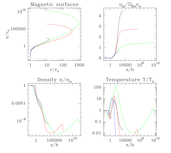
Figure 14: Shape of the magnetic surfaces in the ($r-z$) plane (normalized to the anchoring radius $r_{o}$ (top left) and vertical profiles along the magnetic surfaces of a) the outflow poloidal velocity normalized to the Keplerian speed at $r_{o}$ (top right); b) density normalized to its mid-plane value (bottom left); and c) temperature normalized to its mid-plane value (bottom right). Black lines are for the $p=0.04$ solution, red for $p=0.11$, green for $p=0.3$ and blue for $p=0.45$.

Figure 14 shows several quantities representative of our four densest solutions described in Table 1. Although the global behavior of the wind is qualitatively the same for all solutions (first expansion until recollimation towards the axis), it is quantitatively very different from one solution to another. Indeed, while the maximum wind poloidal speed follows the theoretical scaling with $p$ (or $\lambda)$, the collimation property, as measured for instance by the recollimation radius, does not follow that trend. This is because the asymptotic wind properties depend on the toroidal field component at the disk surface, which is itself quite dependent on the wind thermodynamics. The bumps seen in the temperature profiles are due to the presence of such an heating term. Once the heating disappears, the flow evolves adiabatically with $\gamma=5/3$. The density and temperature at the disk mid-plane at a radius $r$ normalized to the gravitational radius $r_{G}=GM/c^{2}$ write

$$n_{o} = 1.02\times 10^{22}\left(\frac{M}{10M_{\odot}}\right)^{-1}\left(\frac{\varepsilon}{0.01}\right)^{-2}\,\frac{\dot{m}(r)}{m_{s}}r^{-3/2}\mbox{ cm}^{-3}$$ (4)

$$T_{o} = 1.04\times 10^{9}\left(\frac{\varepsilon}{0.01}\right)^{2}\,r^{-1}\,\mbox{K}$$ (5)

for a disk accretion rate $\dot{m}(r)=\dot{M}_{acc}(r)c^{2}/L_{Edd}$ normalized to the Eddington rate $L_{Edd}/c^{2}$. The sonic Mach number $m_{s}$ depends on each MHD solution and is provided in Table 1. Note the accretion rate can also be written as $\dot{m}(r)=\dot{m}_{in}\left(r/r_{in}\right)^{p}$, where $\dot{m}_{in}$ is the normalized accretion rate at the ISCO $r_{in}$.

In practice, if one measures the wind density as the density $n_{SM}$ at the SM point, one would get

$$n_{SM}=5.57\,10^{17}\dot{m}_{in}\left(\frac{r_{in}}{6}\right)^{3/2}\left(\frac{M}{10M_{\odot}}\right)^{-1}\left(\frac{r}{r_{in}}\right)^{p-3/2}\mbox{ cm}^{-3}$$ (6)

for the $p=0.3$ solution which has a ratio $n_{SM}/n_{o}\simeq 6.4\,10^{-3}$ at $z_{SM}=0.78h$ (Figure 14) and assuming $r_{in}=6$ for simplicity.

Note finally that our modeling of wind signatures requires a steady outflow settled from some innermost radius $r_{min}$ to an outer radius $r_{max}$. Mass conservation then implies a total mass loss in the winds of

$$2\dot{M}_{wind}=\dot{M}_{acc}(r_{max})-\dot{M}_{acc}(r_{min})=\dot{M}_{acc}(r_{min})\left(\left(\frac{r_{max}}{r_{min}}\right)^{p}-1\right)$$ (7)

which depends on the radial extent $r_{max}/r_{min}$, the local ejection efficiency $p$ and the disk accretion rate $\dot{M}_{acc}(r_{min})$ at $r_{min}$. It must be realized that neither $p$ nor $\dot{M}_{acc}(r_{min})$ should be the same in these outer regions and in the innermost disk regions where the luminosity is emitted. If one assumes for instance that $p=0$ between $r_{in}$ and $r_{min}$, then of course $\dot{M}_{acc}(r_{min})=\dot{M}_{acc}(r_{in})$. But if another MHD solution is settled below $r_{min}$, say a JED with a different ejection efficiency $p^{\prime}<p$, then one gets $\dot{M}_{acc}(r_{in})=\dot{M}_{acc}(r_{min})\left(\frac{r_{in}}{r_{min}}\right)^{p^{\prime}}$. That would translate in a mass loss in the winds

$$\frac{2\dot{M}_{wind}}{\dot{M}_{acc}(r_{in})}=\left(\frac{r_{min}}{r_{in}}\right)^{p^{\prime}}\left(\left(\frac{r_{max}}{r_{min}}\right)^{p}-1\right)$$ (8)

that could well be much larger than the accretion rate onto the black hole inferred from the disk luminosity. This could be even worse if the disk is not in steady-state, since the accretion time scale for material at $r_{min}$ to reach $r_{in}$ is much larger than days. As a consequence, the outer regions are always in advance with respect to the innermost regions.

Appendix B Caveats

Let us now provide some words of caution. We already stressed that the outcome of our solutions are highly dependent on the heating function, which has been here simply prescribed. Although our magneto-thermal winds do provide good candidates for explaining BHB wind properties, a thorough investigation of the plasma ionisation and thermodynamic states must be undergone. One should indeed verify whether irradiation from the central disk regions can provide the required heating function and how it would affect the MHD solution.

Another major element of uncertainty is related to the properties of the MHD turbulence. Many efforts have been done this last decade to better assess the properties of turbulence in sheared flows threaded by a large scale vertical magnetic field. While most of them were actually focused on measuring the anomalous viscosity $\nu_{v}$, only few works attempted to measure also the magnetic diffusivity $\nu_{m}$ (see Sect. 6 in Jacquemin-Ide, Ferreira & Lesur (2019) and references therein). While our choice of magnetic diffusivity and magnetic Prandle number is consistent with these simulations, our value of $\chi_{m}$ is not. Indeed, Lesur & Longaretti (2009) and Gressel & Pessah (2015) measure a $\chi_{m}\sim 1$. This value is inconsistent with our more massive solutions. Nonetheless, we stress that massive solutions with $p\sim 0.3$ have been computed in Jacquemin-Ide, Ferreira & Lesur (2019). Furthermore, the asymptotic properties of those solutions are analogous to the ones of the solutions presented here.

Finally, one should also note that our dense wind solutions rely on the existence of a large scale magnetic field with a value not too far from equi-partition, namely a disk magnetization $\mu$ varying from 0.06 to 0.4 (see Table 1). Such a large value for the magnetization is better related to a Jet Emitting Disk (JED) than a Standard Accretion Disk (SAD), where values as small as $10^{-3}$ or less are expected for $\mu$ (Pessah et al., 2007; Zhu & Stone, 2018).

It turns out that disks with such a small magnetization can nevertheless drive winds, thanks to the help of the magneto-rotational instability acting at the disk surface. This has been demonstrated by Jacquemin-Ide, Ferreira & Lesur (2019), although only in the case of isothermal flows. They showed that a smaller disk magnetization naturally provides winds with a larger $p$ (as high as $\sim 0.3$), without the need of any extra heat deposition (see their Fig 7). The final outcome of such winds is however very similar to near equi-partition models, with a refocusing towards the axis as shown here. Looking for the wind signatures of such new solutions is postponed to future work. We note however that reaching values larger than $p>0.3$ may, nevertheless require some heat deposition at the disk surface.

Given all the caveats listed above, our work must be seen as a proof of concept of magneto-thermal winds launched from the outskirts of accretion disks and, thereby, as the possible presence of a large scale vertical magnetic field threading the disk in these outer regions.

Appendix C Athena simulations with varying ejection index and line of sight

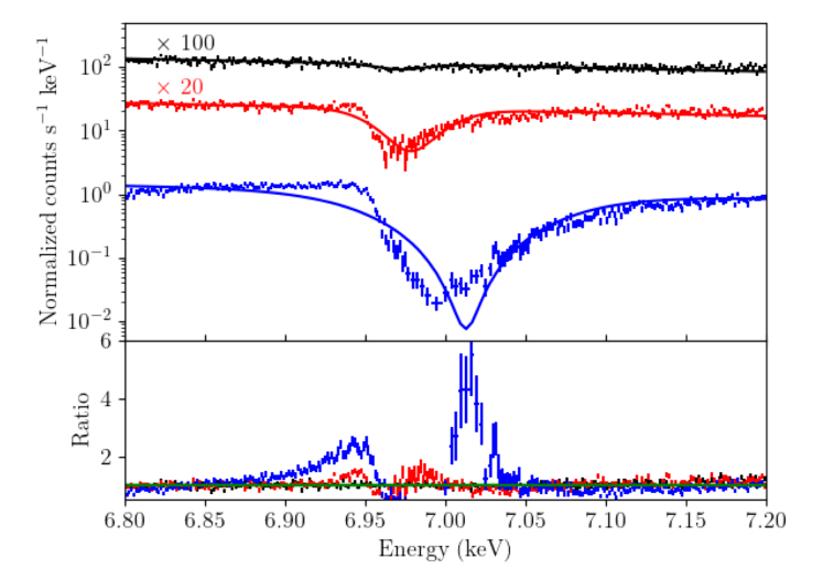
Figure 15: Checking Athena simulations’ sensitivity towards variation of the ejection index ($p$). The source is assumed to have a 2-10 keV flux of 100 mCrab and is ‘observed’ for 100 ks. Top: Variation of the line profile for different $p$ values (black - top: p=0.1, red - middle: p=0.3, blue - bottom: p=0.45). The inclination angle is fixed to $i=20^{\circ}$ (for p=0.1 and 0.3) and $25^{\circ}$ (for p=0.45). $\rm{r_{o}|_{max}}=10^{6}r_{G}$. The solid lines are the best fit with a pow+gau model in xspec. For clarity data and model have been multiplied by 100 for p=0.1 and 20 for p=0.3. Bottom: Corresponding ratios data/model.

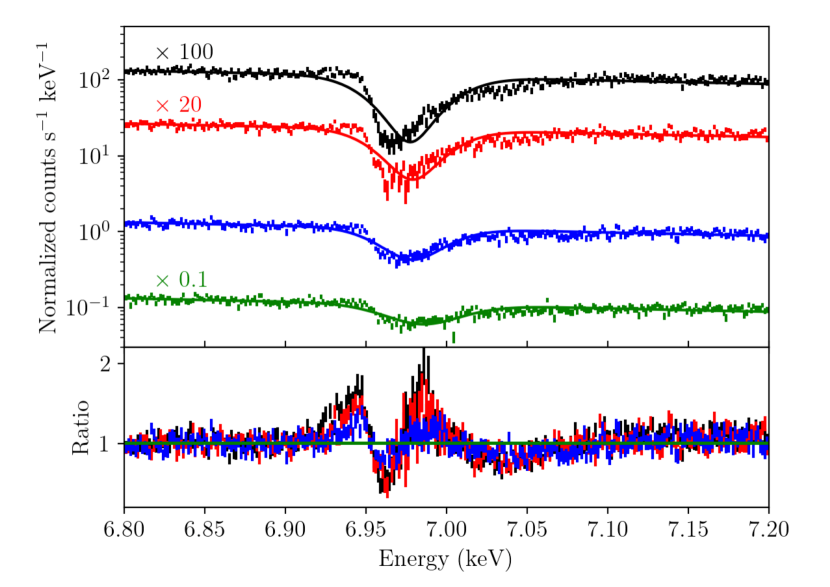
Figure 16: Checking Athena simulations’ sensitivity towards variation of the line-of-sight angles. The source flux and exposure time of observation are the same as used for Figure 15. Top: Variation of the line profile for different LOS angle values (black - top: 15^∘, red - second from top: 20^∘, blue - third from top: 30^∘, green - bottom: 40^∘). The ejection parameter $p=0.3$. $\rm{r_{o}|_{max}}=10^{6}r_{G}$. The solid lines are the best fit with a pow+gau model in xspec. For clarity data and model have been multiplied by 100 for i=15^∘, 20 for i=20^∘ and 0.1 for i=40^∘. Bottom: Corresponding ratios data/model.

C.1 Effect of the ejection parameter

We have reported in Figure 15 the different line profiles of Fe XXVI for different ejection parameters (0.1, 0.3 and 0.45) but assuming same/similar angle of the line-of-sight of $i\sim 20^{\circ}$ and $\rm{ro|_{max}}=10^{6}r_{G}$. We had to use the $i=23^{\circ}$ line-of-sight for the $p=0.45$ MHD model because below this angle the outflow gas is optically thick. As expected the absorption lines are stronger for larger ejection efficiency parameter $p$. A fit with a simple Gaussian absorption line (solid lines in the top panel of Figure 15) show clear residuals for $p>0.1$ (bottom of Figure 15) mainly due to the asymmetry of the line profiles. This asymmetry looks larger when $p$ increases, which can be explained by the larger range of velocity covered by the ”large p” solution (see Figure 2). The absorption line profile peaks also at higher energy (stronger blueshift) for higher ”p”. This profile results from the convolution of the absorption all along the LOS. Then it depends on the subtle combination of the ion density and plasma velocity along the LOS. Now, as just said, larger ”p” solution starts at lower radii and consequently they include higher density and higher velocity parts of the plasma. This explains the stronger blueshift observed.

C.2 Effect of the line-of-sight angle

We have reported in Figure 16 the different line profiles of Fe XXVI for different inclination angles of the LOS (15, 20, 30 and 40 degrees) but assuming now a constant ejection parameter $p$=0.30. We still assume $\rm{ro|_{max}}=10^{6}r_{G}$. The closer the LOS to the disk (i.e. the smaller the LOS inclination) stronger the absorption line and more asymmetric the line profile, as expected because the wind density increases when approaching the disk surface. Beyond $i=30^{\circ}$ line asymmetry is not detected, even if the line can be detected at $i=40^{\circ}$. We do not see a changing blueshift of the Gaussian fit line, as clearly as it was seen during $p$ variation (see Figure 15). That is because, change of the LOS inclination results in small change of the velocity range of the absorbing material.

The absorption line remains detectable even at quite high LOS inclination in the example shown in Figure 16. This is due to the large ejection parameter used i.e. p=0.3. The expected absorption features are quite strong. A smaller $p$ solution (e.g. $p=0.1$) produces absorption features which weaken rapidly when the LOS inclination increases (see Figure 6 left).

References

- Allende Prieto et al. (2001) Allende Prieto, C., Lambert, D.L., & Asplund, M., 2001, ApJ, 556, L63
- Allende Prieto et al. (2002) Allende Prieto, C., Lambert, D.L., & Asplund, M., 2002, ApJ, 573, L137
- Arnaud (1996) Arnaud, K. A. 1996, ASPC, 101, 17
- Barret et al. (2018) Barret, D. et al. 2018, Proceedings of the SPIE, Volume 10699, id. 106991G
- Bianchi et.al. (2017) Bianchi, S.; Ponti, G.; Muñoz-Darias, T.; Petrucci, P.-O. 2017, MNRAS, 472, 245
- Blandford & Payne (1982) Blandford, R. D.; Payne, D. G. 1982, MNRAS, 199, 883
- Blum et al. (2010) Blum, J. L.; Miller, J. M.; Cackett, E.; Yamaoka, K.; Takahashi, H.; Raymond, J.; Reynolds, C. S.; Fabian, A. C. 2010, ApJ, 713, 1244
- Casse & Ferreira (2000a) Casse, F.; Ferreira, J. 2000, A&A, 353, 1115
- Casse & Ferreira (2000b) Casse, F.; Ferreira, J. 2000, A&A, 361, 1178
- Chakravorty et al. (2008) Chakravorty, S., Kembhavi, A.K., Elvis, M. & Ferland, G., Badnell, N. R. 2008, MNRAS, 384L, 24
- Chakravorty et al. (2009) Chakravorty, S., Kembhavi, A.K., Elvis, M. & Ferland, G., 2009, MNRAS, 393, 83
- Chakravorty et al. (2012) Chakravorty, S., Misra, R., Elvis, M., Kembhavi, A.K., & Ferland, G., 2009, MNRAS, 393, 83
- Chakravorty et al. (2013) Chakravorty, S., Lee, J. C., Neilsen, J. 2013, MNRAS, 436, 560
- Chakravorty et al. (2016) Chakravorty, S.; Petrucci, P.-O; Ferreira, J. et al. 2016, A&A, 589, 119
- Contopoulos & Lovelace (1994) Contopoulos, J., & Lovelace, R. V. E. 1994, ApJ, 429, 139
- Dauser et al. (2019) Dauser, T. et al. 2019, A&A, 630, 66
- Diaz Trigo et al. (2013) Diaz Trigo, M; Miller-Jones, J.C.A.; Migliari, S; Broderick, J.W.; Tzioumis, T; 2013, Nature, 504, 260
- Done, Wardinski & Giellinski (2004) Done, C.; Wardinski, G. & Giellinski, M. 2004, MNRAS, 349, 393
- Ferland et al. (1998) Ferland, G. J.; Korista, K. T.; Verner, D. A.; Ferguson, J. W.; Kingdon, J. B.; Verner, E. M. 1998, PASP, 110, 761
- Ferreira & Pelletier (1993) Ferreira, J., & Pelletier, G. 1993, A&A, 276, 625
- Ferreira & Pelletier (1995) Ferreira, J.; Pelletier, G. 1995, A&A, 295, 807
- Ferreira (1997) Ferreira, J. 1997, A&A, 319, 340
- Ferreira (2004) Ferreira, J.; Casse, F. 2004, ApJ, 601L, 139
- Ferreira et al. (2006) Ferreira, J.; Petrucci, P.-O.; Henri, G.; Saugé, L.; Pelletier, G. 2006, A&A, 447, 813
- Frank, King & Raine (2002) Frank, J., King, A., & Raine, D. 2002, Accretion Power in Astrophysics (3rd ed.; Cambridge: Cambridge Univ. Press)
- Fukumura et al. (2010a) Fukumura, K.; Kazanas, D.; Contopoulos, I.; Behar, E. 2010, ApJ, 715, 636
- Fukumura et al. (2010b) Fukumura, K.; Kazanas, D.; Contopoulos, I.; Behar, E. 2010, ApJ, 723L, 228
- Fukumura et al. (2014) Fukumura, K.; Tombesi, F.; Kazanas, D.; Shrader, C.; Behar, E.; Contopoulos, I. 2014, ApJ, 780, 120
- Fukumura et al. (2015) Fukumura, K.; Tombesi, F.; Kazanas, D.; Shrader, C.; Behar, E.; Contopoulos, I. 2015, ApJ, 805, 17
- Fukumura et al. (2017) Fukumura, K.; Kazanas, D.; Shrader, C.; Behar, E.; Tombesi, F.; Contopoulos, I. 2017, NatAs, 1E, 62
- Fukumura et al. (2021) Fukumura, K.; Kazanas, D.; Shrader, C.; Tombesi, F.; Kalapotharakos, C.; Behar, E. 2021, ApJ, 912, 86
- Garcia et al. (2001) Garcia, P. J. V.; Ferreira, J.; Cabrit, S.; Binette, L. 2001, A&A, 377, 589
- Gressel & Pessah (2015) Gressel, O. ; Pessah, M. E. 2015, ApJ, 810, 59
- Higginbottom & Proga (2015) Higginbottom, N.; Proga, D. 2015, ApJ, 807, 107
- Jacquemin-Ide, Ferreira & Lesur (2019) Jacquemin-Ide, J.; Ferreira, J.; Lesur, G. 2019, MNRAS, 490, 3112
- Jacquemin-Ide, Lesur & Ferreira (2021) Jacquemin-Ide, J.; Lesur, G. & Ferreira, J. 2021, A&A, 674, 192
- Kallman (2004) Kallman, T. 2004 arxiv:040161174
- Kallman et al. (2009) Kallman, T. R.; Bautista, M. A.; Goriely, S.; Mendoza, C.; Miller, J. M.; Palmeri, P.; Quinet, P.; Raymond, J. 2009, ApJ, 701, 865
- King et al. (2012) King, A. L. et al. 2012, ApJ, 746L, 20
- Kubota et al. (2007) Kubota et al. 2007, PASJ, 59S, 185
- Lee et al. (2002) Lee, J. C. and Reynolds, C. S. and Remillard, R. and Schulz, N. S. and Blackman, E. G. and Fabian, A. C. 2002, ApJ, 567, 1102
- Lesur & Longaretti (2009) Lesur, G.; Longaretti, P. -Y. 2009, A&A, 504, 309
- Leutenegger et al. (2018) Leutenegger, M.A. et al. 2018, J. Astron. Telescopes Instruments, and Systems 4(2), 021407
- Mitsuda et al. (1984) Mitsuda, K. et al. 1984, PASJ, 36, 741
- Makoto et al. (2018) Makato, T. et al. 2018, Proc. SPIE, Volume 10699, id. 1069922
- Makishima et al. (1987) Makishima, K.; Maejima, Y.; Mitsuda, K.; Bradt, H. V.; Remillard, R. A.; Tuohy, I. R.; Hoshi, R.; Nakagawa, M. 1986, ApJ, 308, 635
- Marcel et al. (2018a) Marcel, G. et al. 2018, A&A, 615, 57
- Marcel et al. (2018b) Marcel, G. et al. A&A, 2018, 617, 46
- Marcel et al. (2019) Marcel, G. et al. 2019, A&A, 626, 115
- Marcel et al. (2020) Marcel, G. et al. 2020, A&A, 640,18
- Miller et al. (2004) Miller et al. 2004, ApJ, 601, 450
- Miller et al. (2006) Miller, J. M.; Raymond, J.; Homan, J.; Fabian, A. C.; Steeghs, D.; Wijnands, R.; Rupen, M.; Charles, P.; van der Klis, M.; Lewin, W. H. G. 2006, ApJ, 646, 394
- Miller et al. (2008) Miller, J. M. and Raymond, J and Reynolds, C. S. and Fabian, A. C. and Kallman, T. R. and Homan, J. 2008, ApJ, 680, 1359
- Miller et al. (2012) Miller et al. 2012, ApJ, 759L, 6
- Morrison & McCammon (1983) Morrison, R.; McCammon, D. 1983, ApJ 270, 119
- Neilsen & Lee (2009) Neilsen, J; Lee, J. C. 2009, Natur, 458, 481
- Neilsen et al. (2011) Neilsen, J.; Remillard, R. A.; Lee, J. C. 2011, ApJ, 737, 69
- Neilsen & Homan (2012) Neilsen, J.; Homan, J. 2012, ApJ, 750, 27
- Neilsen et al. (2016) Neilsen, J.; Rahoui, F.; Homan, J.; Buxton, M. 2016, ApJ, 822, 20
- Peterson (1997) Peterson, B. M. 1997, An Introduction to Active Galactic Nuclei. Cambridge Univ. Press, Cambridge.
- Pessah et al. (2007) Pessah, M.E. ; Chan, C.; Psaltis, D. 2007, Apj, 668, 51
- Petrucci et al. (2010) Petrucci, Pierre-Olivier; Ferreira, Jonathan; Henri, Gilles; Malzac, J.; Foellmi, C. 2010, A&A, 522, 38
- Petrucci et al. (2021) Petrucci, Pierre-Olivier; et al. 2021, A&A, 649A, 128
- Ponti et al. (2014) Ponti, G.; Munoz-Darias, T; Fender, R.P. 2014, MNRAS, 444, 1829
- Ponti et al. (2012) Ponti, G.; Fender, R. P.; Begelman, M. C.; Dunn, R. J. H.; Neilsen, J.; Coriat, M. 2012, MNRAS, 422L, 11
- Remillard & McClintock (2006) Remillard, R. A. and McClintock, J. E. 2006, Annu. Rev. Astron. Astrophys. 44, 49
- Schulz & Brandt (2002) Schulz, N. S.; Brandt, W. N. 2002, ApJ, 572, 971
- Shidatsu, Done & Ueda (2016) Shidatsu, M.; Done, C.; Ueda, Y. 2016, ApJ, 823, 159
- Tarter et al. (1969) Tarter, C.B., Tucker, W. & Salpeter, E.E., 1969, ApJ 156, 943
- Tomaru et al. (2020) Tomaru, R.; Done, C.; Ohsuga, K.; Odaka, H.; Takahashi, T. 2020, MNRAS, 497, 4970
- Ueda et al. (2004) Ueda, Y.; Murakami, H.; Yamaoka, K.; Dotani, T.; Ebisawa, K. 2004, ApJ, 609, 325
- Ueda et al. (2009) Ueda, Y. and Yamaoka, K. and Remillard R. A. 2009, ApJ, 695, 888.
- Ueda et al. (2010) Ueda, Y. et al. 2010, ApJ, 713, 257
- Vlahakis et al. (2000) Vlahakis, N.; Tsinganos, K.; Sauty, C. & Trussoni, E. 2000, MNRAS, 318, 417,
- Witthoeft (2011) Witthoeft et al. 2011, ApJS, 196, 7.
- Zhu & Stone (2018) Zhu, H.; & Stone, J.M. 2018, ApJ, 857, 34