Blackbody temperature of 200+ stellar flares observed with the CoRoT satellite

Abstract

We estimated blackbody temperature for 209 flares observed at 69 F-K stars, significantly increasing the number of flare temperature determinations. We used the Blue and Red channels obtained by the 27 cm telescope of the CoRoT satellite at high cadence and long duration. The wavelength limits of the channels were estimated using spectra from the Pickles library for the spectral type and luminosity class of each star, provided by the Exodat Database. The temperatures were obtained from the flare energy Blue-to-Red ratio, using the flare equivalent duration and stellar flux in both channels. The expected value of the analyzed flares is equal to 6,400 K with a standard deviation of 2,800 K, where the mean stellar spectral type, weighted by the number of flares in each spectral subclass, is equal to G6. Contrary to our results, a stellar white-light flare is often assumed to emit as a blackbody with a temperature of 9,000 K or 10,000 K. Our estimates agree, however, with values obtained for solar flares. The GAIA G-band transmissivity is comparable to that of the CoRoT White channel, which allows us to calibrate the flares to the Gaia photometric system. The energy in the G band of the analyzed flares varies between $10^{32}$ and $10^{37}$ erg and the flare area ranges from 30 $\mu$sh to 3 sh (solar hemisphere). The energy release per area in a flare is proportional to $T_{\rm flare}^{2.6}$, at least up to 10,000 K.

1 Introduction

Although solar flares are more noticeable in UV and X-ray observations, they emit in a broad range of electromagnetic radiation. In fact, most of the radiated flare energy emerges at visible and UV wavelengths (Woods et al., 2006; Kretzschmar, 2011). Flares observed in the visible spectrum are called white-light flares (WLFs). Solar WLFs are generally rare events to observe, mainly due to the low contrast with the solar disk (Lin & Hudson, 1976; Jess et al., 2008).

High-cadence, high-precision continuous photometry observations from space (e.g., CoRoT, Kepler, Tess) have made possible extensive observations of stellar flares in the visible on various types of stars. These stellar flares can be up to $\sim$10,000 (or even a million; see Schaefer et al., 2000) times larger than the largest solar flares. Despite this, several statistical studies show that stellar flares have solar-like properties, indicating that they may also be the result of magnetic reconnection events (Namekata et al., 2017, and references within). Fast-rotating stars have higher magnetic activity, as is to be expected from the dynamo theory of magnetic field generation. In fact, it is observed that they have a higher occurrence rate of flares than slow rotators (Shibayama et al., 2013) but not more energetic flares (Maehara et al., 2012). Notsu et al. (2013) found that there is a correlation between spot coverage and flare energy.

Determining the flare temperature provides valuable information that can help to understand the physical processes responsible for the flare emission (e.g. Kowalski et al., 2016). Unfortunately, these space missions only provide information in a single filter passband, not allowing to estimate the temperature of the flare. There are some papers where it was estimated. Hawley & Fisher (1992) analyzed a large flare at the M-dwarf star AD Leo. They obtained a blackbody temperature of 8500$-$9500 K fitting the average surface flux observed at six passbands (Johnson U, B, V, and R and two in the near UV) during the flare. Hawley et al. (2003) analyzed four other flares on AD Leo and obtained similar results ($\sim$9000 K). Kowalski et al. (2013) analyzed 20 flares in 5 M-dwarf stars using high-cadence near-ultraviolet and visible spectra. They observed that all flares present a linear decrease in flux at wavelengths from 4000 to 4800 Å  corresponding to a blackbody temperature between 9000 K and 14000 K. They reported variations in the Balmer jump during the flare that indicate an additional component to the blackbody emission in the near UV range (Kowalski et al., 2019). Howard et al. (2020) used simultaneous observations in the narrow g’-band obtained by a series of small telescopes (Law et al., 2016, Evryscope) and the broadband filter of NASA’s TESS satellite (Ricker, 2014) to estimate the temperature and energy of 47 flares on 27 K5-M5 dwarfs. They found that nearly half of the flares emit above 14,000 K during their peak. However, the temperature of the entire flare varies widely, from 2,600 K to 50,000 K.

Based on these stellar temperature estimations, the WLF spectrum is often described as a blackbody with a temperature between 9,000$-$10,000 K and used to estimate the bolometric energy of the flare (e.g. Maehara et al., 2012; Shibayama et al., 2013; Davenport et al., 2020; Günther et al., 2020; Maehara et al., 2021). A change in the assumed flare temperature may significantly affect the energy-frequency distribution estimate, which is used to model the atmospheric conditions of the planets orbiting the flaring star, that allows to assess the possibility of life and the probability of becoming a candidate for a biosignature survey (e.g. Günther et al., 2020).

For solar WLFs, there is an earlier estimation of a temperature similar to that of the M-dwarf stellar flares, equal to $\sim$9000 K by Kretzschmar (2011). Later, Kerr & Fletcher (2014) estimated temperatures between 5,000 and 6,000 K, Kleint et al. (2016) between $\sim$ 6000 and 6300 K, and Namekata et al. (2017) between 5500 and 7000 K.

In this work, we used the CoRoT color channels to estimate the temperature of more than 200 stellar flares observed in more than 50 stars with different spectral types. We describe in Section 2 the data used and the fitting and equivalent duration estimation of the flares. Section 3 presents the estimation of the limits of the CoRoT color channels that we used in the flare temperature calculation, described in Section 4. As stellar rotation has an effect on stellar activity, the rotation estimate is presented in Section 5, to be compared with the flare temperatures. Finally, in Section 6, we took advantage of the similarity of the CoRoT White channel to the Gaia G band to calibrate the analyzed flares into the Gaia photometric system. In Section 7, we present our conclusions.

2 Data and Methodology

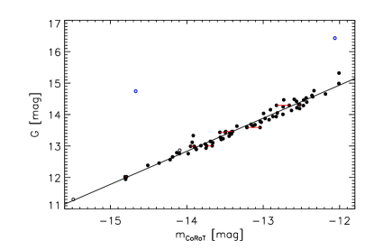
Figure 10: Observed GAIA G magnitude as a function of CoRoT White channel magnitude for all analyzed stars. The three empty black circles are more than 1 arcsec from the nearest star in the GAIA EDR3 catalog. One of the three has $m_{\rm CoRoT}$ = -13.9 mag and is not easily visible in the figure. The two empty blue circles are more than 4$\sigma$ away from the fitted straight line and were also removed from the fitting. The small red horizontal lines link the CoRoT magnitudes of stars that have been observed twice.

CoRoT (Convection, Rotation and planetary Transits) was a space-based mission that obtained precise photometric observations of hundreds of thousands of stars from 2007 to 2012 in two regions of the sky (one toward the galactic center and another toward the Galactic anticenter) $-$ Baglin & CoRot Team (2016). We studied stars observed through the so-called Faint Stars or Exoplanet channel (Ollivier et al., 2016). The stellar images were dispersed by a prism that was in the optical path before the CCDs, producing a low-dispersion spectrum of each star. For about 6000 stars, CoRoT provided not only a light curve integrating the entire photometric mask (called White light curve) but also three light curves dividing the mask into three regions corresponding to different spectral bands whose fluxes were recorded separately (Auvergne et al., 2009). The boundaries within the mask were chosen so that each flux was close to a given fraction of the total flux and corresponds to an integer number of columns on the CCD as the dispersion was done in rows (Fig.10 and 11 in Léger et al., 2009). These color light curves were named Red, Green, and Blue, although its spectral content varies with the shape of the photometric mask used, the star’s apparent magnitude, spectral type, etc (Bordé et al., 2010). The flux in the Green channel is low compared to the others (Borsa & Poretti, 2013) and was not used here due its low signal-to-noise ratio.

Drabent (2012) published a list of 111 flaring stars after analyzing all CoRoT light curves observed until 2010 December (including observational sequence LRa04). We used the light curves for these stars provided by the CoRoT public archive . Three data correction levels for each light curve are provided. We used the most basic (provided by the BAR extension in the FITS files), which does not include correction of jumps or replacement of invalid and missing data (Chaintreuil et al., 2016), as a flare could be misinterpreted as a jump or invalid data. The housekeeping temperature data show jumps (Ollivier et al., 2016) that can affect the light curve and mimic a flare. Thus, we disregard the corresponding time intervals in the analyzed light curves (provided by the keyword ”statusfil” in the BARFILL extension). Although CoRoT observations last 32 s, in most stars, 16 observations are gathered at a cadence of 512 s (Ollivier et al., 2016). Approximately one-third of the analyzed stars have a cadence of 512 s and the remaining have a cadence of 32 s.

We visually inspected each light curve and manually selected the approximate beginning and end of each flare, using FBEYE software developed by Davenport et al. (2014). We fitted each flare and its background using a two-exponential function plus a straight line:

$$F_{\rm local}(t)=F_{\rm bk}(t)+F_{\rm flare}(t)=$$

$$a_{4}+a_{5}t+a_{0}\left\{\begin{array}[]{c}e^{a_{2}(t-a_{1})}\,\,\,,\,\,\,t\,<\,a_{1}\\ e^{-a_{3}(t-a_{1})}\,\,,\,\,\,t\,\geq\,a_{1}\\ \end{array}\right.$$ (3)

observed in each color channel. We applied a least-squares Levenberg–Marquardt minimization algorithm to obtain the best-fit flare parameters and a Maximum likelihood via Monte-Carlo Markov Chain algorithm (Foreman-Mackey et al., 2013) to estimate the uncertainties of the fitted parameters, using the LMFIT Python package. Figure 1 shows a few examples of the fitting. The flare fitted parameters are the flare peak flux ($a_{0}$), the peak flare occurrence time ($a_{1}$), the exponential growth rate ($a_{2}$) and the decay rate ($a_{3}$).

The equivalent duration, ED, of a flare (Gershberg, 1972) is given by:

$${\rm ED}=\int_{0}^{\infty}\frac{F_{\rm flare}(t)}{F_{{\rm qu}}}\,dt=\frac{a_{0}}{F_{\rm qu}}\left(\frac{1}{a_{2}}+\frac{1}{a_{3}}\right)$$ (4)

where $F_{\rm flare}(t)$ is the flux due only to the flare (after removing the background) and $F_{\rm qu}$ is the flux in the quiescent state. As the background varies throughout the flare, we used the background value at the flare peak as the quiescent flux: $F_{\rm qu}=a_{4}+a_{5}\,a_{1}$. Figure 2 shows the equivalent duration obtained for each flare observed in the Blue and Red channels. Only flares for which we obtained an ED greater than 1.5$\sigma$ (where $\sigma$ is the uncertainty in ED) were used here and are shown in the Figure. The ED varies from 2 to 2,000 seconds. There are 209 flares observed in both the Blue and Red channels and a similar number of flares that are visible only in the Red or Blue channel. The mean value of the Blue-to-Red ED ratio and its standard error is equal to 2.36$\pm$0.09 (shown as a green line in Figure 2).

The flare peak flux ($a_{0}$ in Eq. 3) divided by the flux in the quiet state observed in the Blue channel versus in the Red channel is shown in Figure 3. The mean and its standard error of the Blue-to-Red flare peak amplitude ratio normalized by its respective quiet state is equal to 2.75$\pm$0.09 (shown as a green line in Figure 3). The Blue-to-Red full width at half-maximum (FWHM) ratio is close to 1. The flare FWHM ranges from 2 minutes to 2.5 hours.

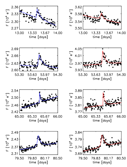
Figure 1: Flare light curves for CoRoT 106048015 obtained in the Blue (left) and Red (right) channels. The solid line shows the fitted model.

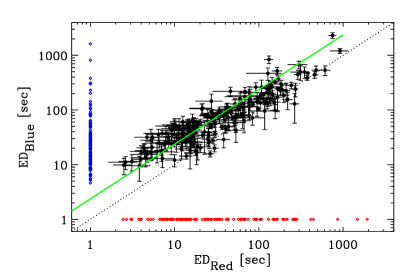
Figure 2: Equivalent duration observed in the Blue channel versus in the Red channel. There are 209 flares observed in both the Red and Blue channels, shown as black circles. A similar number of flares is only seen in the Blue or Red channel, which are shown as small blue and red diamonds, respectively, with the equivalent duration on the other channel set to one. The solid green line is given by ${\rm ED}_{\rm Blue}=2.36\,{\rm ED}_{\rm Red}$.

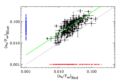
Figure 3: Blue-versus-Red flare peak amplitude normalized by its quiescent state shown as black circles. Flares that are only seen in the Blue or Red channel are shown as small blue and red diamonds, respectively, with the peak amplitude ratio on the other channel set to 0.001. The solid green line corresponds to: (a₀/F_qu)_Blue = 2.75 (a₀/F_qu)_Red.

In our analysis, besides ruling out several flares where the equivalent duration was not well determined (i.e., ${\rm ED}<1.5\sigma$) due to its small duration or amplitude, we also discarded those within a thermal jump or with missing data during the flare. In the end, we accepted 209 flares observed both in the Blue and Red channels. These flares belong to 69 stars, reducing the number of stars in our initial sample.

3 Blue and Red channel wavelength limits

To obtain the chromatic light curves, the observed low-resolution stellar spectrum multiplied by the CoRoT response function was divided into three parts: the Blue band corresponds to the shorter wavelengths, the Red band to the longer ones, and the Green band to intermediate values. Unfortunately, the boundaries that separate the channels vary for each observed star and for each observation period (since the star may be on a different CCD) - Bordé et al. (2010). In this section, we estimate these limits for each light curve: the upper wavelength limit of the Blue channel, $\lambda_{\rm Blue}$, and the lower wavelength limit of the Red channel, $\lambda_{\rm Red}$.

For each star, the spectral type and luminosity class were retrieved from the Exodat Database (Deleuil et al., 2009) - later shown in Table 2. The stellar classification in the Exodat Database was estimated by fitting the apparent magnitude of CoRoT stars (obtained by ground-based multi-color broadband photometric observations) to the spectral flux from the Pickles Stellar Spectral Flux Library (Pickles, 1998). Damiani et al. (2016) reported that the luminosity class is estimated with great significance and that the typical uncertainty on the spectral type is of half a spectral class. We used the spectra from the Pickles Library for the spectral type and luminosity class of the star $s$, $f^{s}_{P}(\lambda)$, to estimate the wavelength limits:

$$\frac{F^{\rm obs}_{{\rm Blue}}}{F^{\rm obs}_{{\rm White}}}(l)=\frac{\int_{0}^{\lambda_{\rm Blue}(l,s)}{\Phi(\lambda)\,\,f_{P}^{s}(\lambda)\,\lambda\,d\lambda}}{\int_{0}^{\infty}{\Phi(\lambda)\,\,f_{P}^{s}(\lambda)\,\lambda\,d\lambda}}$$

$$\frac{F^{\rm obs}_{{\rm Red}}}{F^{\rm obs}_{{\rm White}}}(l)=\frac{\int_{\lambda_{\rm Red}(l,s)}^{\infty}{\Phi(\lambda)\,\,f_{P}^{s}(\lambda)\,\lambda\,d\lambda}}{\int_{0}^{\infty}{\Phi(\lambda)\,\,f_{P}^{s}(\lambda)\,\lambda\,d\lambda}}$$ (5)

where the terms on the left-hand side are the observed average stellar flux ratios for each light curve $l$. $\Phi$($\lambda$) is the CoRoT Response Function for the Faint Stars channel (Auvergne et al., 2009). Most stars $s$ have only one light curve $l$, except for eight of them, which have two light curves observed four years apart. We used the Pickles library UVKLIB, which covers the spectral range 1150$-$25,000 Å. In the library, the fluxes are in units of erg cm^-2 s^-1Å^-1 and the original fluxes in the Pickles V band were normalized to a 0 magnitude in the Vega magnitude system. As the functions on the right-hand side of equations 5 vary smoothly with $\lambda_{\rm Blue}(l,s)$ and $\lambda_{\rm Red}(l,s)$, we can use the error propagation equation (Bevington & Robinson, 2003). The uncertainties of the wavelength limits, $e_{\lambda_{\rm Blue}}(l,s)$ and $e_{\lambda_{\rm Red}}(l,s)$, were estimated dividing the standard error of the mean observed flux ratio by the derivative of the right-hand side expression at the estimated wavelength limit. The uncertainties are very small, they are less than 0.2 Å.

We also included the uncertainty in the stellar classification in the wavelength limit estimation. To be on the safe side, we assumed twice the uncertainty in stellar classification given in Damiani et al. (2016). For each light curve $l$, we estimated the limit of each channel, using all spectra in the Pickles library within plus/minus a spectral class and within plus/minus two luminosity classes of the star $s$: $(\lambda_{\rm Blue}\pm e_{\lambda_{\rm Blue}})(l,s_{i})$ and $(\lambda_{\rm Red}\pm e_{\lambda_{\rm Red}})(l,s_{i})$, $i=1,...,N$. For our stars, there are between 18 and 68 spectra within these uncertainties (18 $\leq N\leq$ 68) and only 7 of the 69 stars have less than 30 spectra. Next we calculated the weighted average limit of the channels for each light curve $l$, $\bar{\lambda}_{\rm Blue}(l)$ and $\bar{\lambda}_{\rm Red}(l)$, where the weight is given by the inverse square of the uncertainty. We estimated the uncertainty in the weighted averages (Bevington & Robinson 2003 and in more detail in the supplement of Kirchner & Allen 2020): $\sigma_{\lambda_{\rm Blue}}(l)$ and $\sigma_{\lambda_{\rm Red}}(l)$. They have a percent uncertainty ranging from 2%$-$5%. The results are shown in Figure 4 (top panel). Later in this paper, we compare our results using these limits (Fig. 4) with limits calculated as described above, but assuming a smaller uncertainty in stellar classification: within plus/minus half a spectral class and within plus/minus one luminosity class. These weighted average limits agree with the previous ones within their uncertainty. As expected, their uncertainties are half of the former ones.

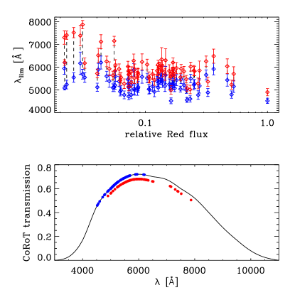
Figure 4: Top panel. Weighted mean of the wavelength limits for each light curve: $\bar{\lambda}_{\rm Blue}(l)$ (blue symbols) and $\bar{\lambda}_{\rm Red}(l)$ (red symbols), as a function of the observed mean stellar flux in the Red channel, $F^{\rm obs}_{{\rm Red}}(l)$, divided by its maximum value among the analyzed light curves. The error bars correspond to the uncertainties in the weighted averages. The limits of a given light curve in the Blue and Red channels are connected by a vertical dashed black line for better visualization. We observe an increase in $\bar{\lambda}_{\rm Red}$ at small values of the stellar Red flux, indicating a narrowing of this channel. We do not observe any variation in the wavelength limits as a function of the Blue or White stellar flux. Bottom panel. The CoRoT Response Function for the Faint Stars channel (Figure 14 in Auvergne et al., 2009) is shown in black. The wavelength limits (from the top panel) are shown in the color of their respective band. The ones for the Red channel are displaced vertically by -0.04 for a better visualization.

According to Rouan et al. (1999), the fraction in each channel should not be far from 20% of the bluest photons for the Blue channel and 65% of the reddest photons for the Red channel. The averages over the analyzed stars of the Blue-to-White and Red-to-White observed flux ratio, measured in electrons, are equal to 0.16$\pm$0.01 and 0.72$\pm$0.01, respectively, where the uncertainties are given by the error of the mean. However, if we calculate the stellar fluxes in units of energy using the right-hand side of Equations 5, but without multiplying by the wavelength, the average ratios are 0.22$\pm$0.01 and 0.63$\pm$0.01, respectively, which agree with the fractions given by Rouan et al. (1999).

4 Effective flare temperatures

We assumed that the spectrum of white-light flares can be described by a blackbody, $B_{\lambda}$, with temperature, $T_{\rm flare}$ (Mochnacki & Zirin, 1980; Shibayama et al., 2013; Günther et al., 2020, and others). Following Shibayama et al. (2013), we can estimate the flare luminosity ($L_{\rm flare}$) observed by CoRoT in the White channel, in photons, as:

$$L_{\rm flare}(t)=A_{\rm flare}(t)\,\,\,\int_{0}^{\infty}\Phi(\lambda)B_{\lambda}(T_{\rm flare})\lambda\,d\lambda$$ (6)

where $A_{\rm flare}(t)$ is the area of the flare as a function of time and $\Phi(\lambda)$ is CoRoT Response Function for the Faint Stars channel (Fig. 4).

The equivalent duration (Equation 4) can be written as:

$${\rm ED}=\frac{1}{L_{\star}}\int_{\rm flare}L_{\rm flare}(t)\,dt.$$ (7)

where $L_{\star}$ is the luminosity of the star observed with the CoRoT White channel. Assuming that the flare area and temperature are constant during the flare (as in Shibayama et al., 2013; Günther et al., 2020) and substituting Equation 6 into Equation 7, we have:

$${\rm ED}=\frac{A_{{\rm flare}}}{L_{\star}}\,\,\Delta t\,\,\,\int_{0}^{\infty}\Phi(\lambda)B_{\lambda}(T_{{\rm flare}})\,\lambda\,d\lambda$$ (8)

where $\Delta t$ is the flare duration. The ratio between the equivalent duration observed in the Blue and Red channels is:

$$\frac{{\rm ED}_{{\rm Blue}}}{{\rm ED}_{{\rm Red}}}=\frac{F_{\rm Red}}{F_{\rm Blue}}\,\frac{\Delta t_{\rm Blue}}{\Delta t_{\rm Red}}\,\,\frac{\int_{0}^{\lambda_{\rm Blue}}{\Phi(\lambda)\,\,B_{\lambda}(T_{{\rm flare}})\,\lambda\,d\lambda}}{\int_{\lambda_{\rm Red}}^{\infty}{\Phi(\lambda)\,\,B_{\lambda}(T_{{\rm flare}})\,\lambda\,d\lambda}}.$$ (9)

We also assumed that the area of the flare is the same in observations using the Blue or the Red channel. The energy of a flare, $E$, is defined as the product of its equivalent duration (ED) and the quiescent luminosity of the star $L_{\star}$ (e.g. Shibayama et al., 2013; Hawley et al., 2014; Rodríguez Martínez et al., 2020; Günther et al., 2020). Using Equation 9, the energy ratio is given by:

$$\frac{E_{{\rm Blue}}}{E_{{\rm Red}}}=\frac{{\rm ED}_{{\rm Blue}}}{{\rm ED}_{{\rm Red}}}\,\frac{F_{\rm Blue}}{F_{\rm Red}}=$$

$$\,\frac{\Delta t_{\rm Blue}}{\Delta t_{\rm Red}}\,\,\frac{\int_{0}^{\lambda_{\rm Blue}}{\Phi(\lambda)\,\,B_{\lambda}(T_{{\rm flare}})\,\lambda\,d\lambda}}{\int_{\lambda_{\rm Red}}^{\infty}{\Phi(\lambda)\,\,B_{\lambda}(T_{{\rm flare}})\,\lambda\,d\lambda}}.$$ (10)

The flare duration was calculated using the flare fitted parameters (Equation 3). The analyzed flares have, on average, the same duration in the Blue and Red channels. We used Equation 10 to estimate $T_{\rm flare}(k)$, for each flare $k$ observed in a given light curve $l$, since it is the only unknown parameter in the equation:

$$\frac{E_{{\rm Blue}}}{E_{{\rm Red}}}(l,k)=\frac{{\rm ED}_{{\rm Blue}}}{{\rm ED}_{{\rm Red}}}(k)\,\cdot\,\frac{F^{\rm obs}_{{\rm Blue}}}{F^{\rm obs}_{{\rm Red}}}(l)=$$

$$\frac{\int_{0}^{\bar{\lambda}_{\rm Blue}(l)}{\Phi(\lambda)\,\,B_{\lambda}[T_{{\rm flare}}(k)]\,\,\lambda\,d\lambda}}{\int_{\bar{\lambda}_{\rm Red}(l)}^{\infty}{\Phi(\lambda)\,\,B_{\lambda}[T_{{\rm flare}}(k)]\,\,\lambda\,d\lambda}}.$$ (11)

The flare energy ratio as a function of $T_{\rm flare}$, given by the ratio of integrals on the right-hand side of Equation 11, is shown in Figure 5. It varies smoothly with $T_{\rm flare}$ for a given pair of wavelength limits: $\bar{\lambda}_{\rm Blue}(l)$ and $\bar{\lambda}_{\rm Red}(l)$. Using the error propagation equation, we estimated the flare temperature uncertainty, $\sigma_{T_{\rm flare}}(k)$, by dividing the uncertainty of the observed flare energy ratio, ED_Blue/ED${}_{{\rm Red}}(k)\,\cdot F_{{\rm Blue}}/F_{{\rm Red}}(l)$, by the derivative of the right-hand side expression at the estimated flare temperature. As seen in Fig. 5, the slope of the flare energy rate tends to zero as the flare temperature increases. Therefore, the estimated uncertainty in the flare temperature increases with the flare temperature. This is a consequence of using observations in the visible range to estimate high temperatures. According to Wien’s law, a blackbody with a temperature of 10,000 K will have its maximum emission at 2900 Å  and outside the CoRoT Response Function (Fig. 4).

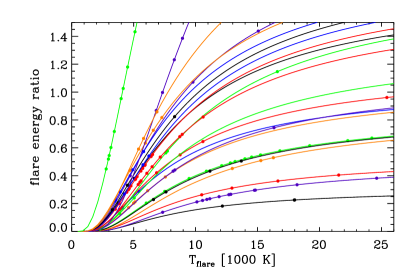
Figure 5: Flare energy ratio, $E_{\rm Blue}/E_{\rm Red}$, as a function of flare temperature, $T_{\rm flare}$, given by the rightmost term in Equation 11. Each color is for a given light curve $l$. For a better visualization, only light curves with 3 or more observed flares are plotted. The full circles are the observed flare energy ratio and the correspondent estimated flare temperature, $T_{\rm flare}$(k).

To take into account the uncertainty in the estimated wavelength limits, we added noise to the flare temperature calculation. For each pair $\bar{\lambda}_{\rm Blue}(k)$ and $\bar{\lambda}_{\rm Red}(k)$, we generated 1000 input pairs by adding different random realizations of Gaussian noise with a standard deviation given by $\sigma_{\lambda_{\rm Blue}}(l)$ and $\sigma_{\lambda_{\rm Red}}(l)$, respectively. The final estimate of the flare temperature is the weighted average of 1000 estimates obtained using perturbed input wavelength limits: $(\bar{T}_{\rm flare}\pm\sigma_{T_{\rm flare}})(k)$ $-$ Table 2. The percent uncertainty of the weighted mean ranges from 10%$-$40%. Figure 6 (first row) shows the average flare temperatures for each star (in the same color) in ascending order of the average temperature of the flares in a given star. A total of 70% of the analyzed stars have only one or two flares. Those with two or more flares often have similar flare temperatures. Figure 7 shows the temperatures for stars with 6 or more flares.

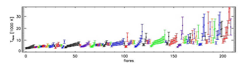
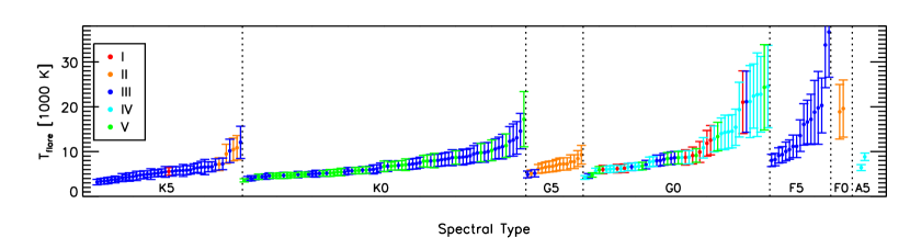
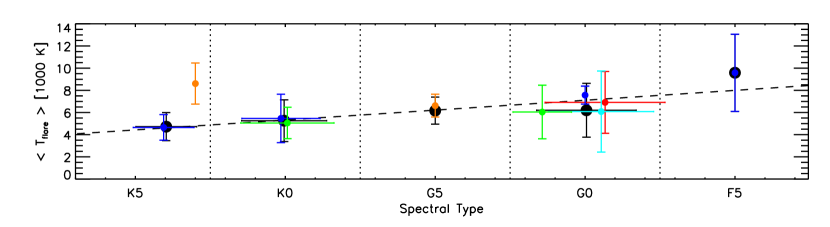
Figure 6: 1st row: Weighted mean flare temperatures, $\bar{T}_{\rm flare}$(k), of the 209 flares and their standard deviation, $\sigma_{T_{\rm flare}}(k)$. The flares in a given star are shown in the same color. They are ordered with increasing mean temperature of all flares in a given star. 2nd row: Same as the first row plot, but as function of spectral type, going from late to early type stars, in intervals of half a spectral class. The spectral type at the center of each interval is shown at the bottom of the plot. Inside each spectral class interval, the flare temperatures are in ascending order. The different colors are for the different luminosity classes. 3rd row: Weighted average of the temperature of the flares versus the average of the spectral subclass corresponding to the flares within each interval of half a spectral class. The averages for a given luminosity class, when there are 4 or more flares, are shown in different colors (as in the 2nd-row panel). The averages including all luminosity classes are shown in black and their linear regression is given by the black dashed line. The vertical error bars correspond to the standard deviation of the flare temperature weighted average and the horizontal error bars to the standard deviation of the average of the spectral subclass. The absence of a horizontal bar means that only one spectral type was used in the temperature averaged.

Figure 7: Weighted mean flare temperature, $\bar{T}_{\rm flare}$(k), as in Figure 6 (1st-row panel), for stars with 6 or more flares. The CoRoT ID and stellar spectral type are shown in each panel. The vertical dashed lines on four of the stars separate the flares obtained in different observation sequences: during 2008 and 2012. The vertical axis range is twice as large for the first three stars as for the others.

We checked whether there is any dependence of the flare temperature with stellar spectral type. Figure 6 (2nd row) shows the flare temperatures in intervals of half-spectral type, where within each interval the temperatures are in ascending order and the flares in each luminosity class are in a different color. We calculated the weighted average of the flare temperature over each interval which is shown in the 3rd-row panel. The average over all luminosity classes are shown in black. The average flare temperature, including all luminosity classes (black circles), ranges from (4700 $\pm$ 1300) K for spectral type K4 to (9600 $\pm$ 3500) K for F5 type and the slope of the linear regression is equal to (1800$\pm$1400) K per spectral type. The Pearson correlation coefficient (of the black circles) is 0.9 which has only a 5% probability of not being correlated (Bevington & Robinson, 2003). We calculated the correlation coefficient after adding normally distributed random numbers with the same standard deviation of the mean flare temperature (shown in the 3rd-row panel) to examine the effect of their uncertainty on the correlation. The average Pearson coefficient and its standard deviation of 10,000 instances is: (0.58$\pm$0.37) and the probability of not being correlated is 30%.

Next, we analyzed the frequency distribution of the estimated flare temperatures. Figure 8 shows the histogram (solid black line) of the 209 $\bar{T}_{\rm flare}(k)$ plotted in Fig. 6 (1st row). We estimated the probability density function (PDF) using the kernel density estimator (KDE) method (Silverman, 1986) - with a Gaussian kernel - without taking into account flare temperature uncertainties. It agrees well with the histogram after the PDF was multiplied by the number of flares and size of histogram bin (full red line). The kernel has an optimal window width (given by equations 3.30 and 3.31 in Silverman, 1986) equal to 983 K, which is used as the histogram bin width (solid black line). However, when including the flare temperature uncertainties in the estimation, the normalized PDF (blue line) has its maximum shifted toward a smaller flare temperature, with a mode equal to 5,300 K. The distribution no longer has a long tail, and the width of the highest density interval (HDI) is narrower by 33%. This is to be expected, since flares with high temperatures have greater uncertainties, as mentioned earlier. In Table 1, we summarize the characteristics of the distributions (called ”A”). They give us some indication of the upper and lower limits of the flare temperature distribution. The average spectral type of all flaring stars, weighted by the number of flares observed in stars in each spectral subclass, is equal to G6.

As mentioned in Section 3, we also calculated wavelength limits using a smaller uncertainty in the stellar classification (i.e., within plus/minus half a spectral class and within plus/minus one luminosity class). Reestimating $\bar{T}_{\rm flare}$ in the same way as described above, but with these wavelength limits, we find that the new $\bar{T}_{\rm flare}$ are systematically larger than before by a small amount, which is, on average, equal to 1 $\sigma_{T_{\rm flare}}$. Their histogram is shown in Fig. 8 by a black dashed line. Their normalized PDF calculated without including the uncertainties (dashed red line) and including the uncertainties (not shown in the figure) have modes and mean values that are a few percent larger than before (labeled ”B” in Table 1).

We did a simple exercise to see how higher-than-observed flare temperatures would show in the results of our analysis. We artificially increased the value of the observed equivalent duration ratio given as input to Eq. 11 to analyze the corresponding increase in $\bar{T}_{\rm flare}(k)$. After increasing the equivalent duration ratio by 50% and 100% and repeating the calculation of $\bar{T}_{\rm flare}(k)$ as described above, the estimated PDF is shifted by approx. 20% (green solid line) and $\sim$40% (green dashed line) in $T_{\rm flare}$, respectively. While the width of 75% HDI increases by $\sim$40 % and $\sim$80 %, respectively. A wide HDI width indicates a greater uncertainty in the parameter determination, which could be explained by the difficulty of observations in the visible range to measure large flare temperatures.

Table 1: PDF properties of our main results (‘A’). The table also shows for comparison the PDF properties of the results obtained assuming a smaller uncertainty in the stellar classification (‘B’) and those obtained by the arbitrary multiplication of the equivalent duration of the flare by 1.5 (‘1.5$\times$’) and 2 ( ‘2.0$\times$’). The columns are as follows: (1) PDF used; (2) y (yes) or no to indicate whether or not the flare temperature uncertainties were included in the PDF estimate; (3) colored lines as plotted in Figure 8 (if dashed, it is labeled $-$); (4) mode; (5) mean value (or expected value); (6) standard deviation of the mean; (7) lower and (8) upper limits in the 75% HDI. All values are given in Kelvin.

		line	mode	mean	$\sigma$	lower	upper
A	y	blue	5300	6400	2800	3400	8100
B	y	none	5400	6600	2700	3500	8200
A	no	red	5800	8400	4600	3300	10300
B	no	$-$red	6200	8700	4700	3700	10700
1.5$\times$	no	green	7200	10200	5000	3900	13600
2.0$\times$	no	$-$green	8400	12100	5700	4600	17300
1.5$\times$	y	none	6300	7700	3600	3400	10000
2.0$\times$	y	none	7100	9100	4500	3500	11900

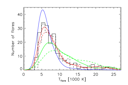
Figure 8: Histogram (solid black line) of the mean flare temperature, $\bar{T}_{\rm flare}$, for all 209 flares in intervals of 983 K, which is close to the median of flare temperature uncertainty. The PDF obtained with the kernel density estimation (Silverman, 1986) (using a Gaussian kernel) with and without taking into account flare temperature uncertainty are shown as blue and red lines, respectively. The histogram shown with dashed black line is for mean flare temperatures obtained using wavelength limits estimated assuming a smaller uncertainty in the stellar classification used (i.e., half a spectral type and one luminosity class). It is slightly displaced horizontally for a better visualization. Its PDF estimated, without taking into account the uncertainty, is shown by the dashed red line. The green solid and dashed lines show the PDF (without taking into account flare temperature uncertainty) obtained by increasing the input ED by 50% and 100%, respectively. The probability density functions plotted here were normalized to be compared with the histograms, they were multiplied by the number of flares (209) and size of histogram bin (983 K).

5 Rotation

As suggested by dynamo theories and obtained from observations of cool stars, of any spectral type, the stellar activity increases with the rate of rotation and even more so with the Rossby Ro number, where small values of Ro indicate very active stars (Donati & Landstreet, 2009). On the other hand, intermediate- and high-mass stars exhibit virtually no intrinsic variability. We calculated the stellar rotation to search for a correlation with flare temperature.

The presence of active regions on a star’s surface produces periodic variations in stellar observed brightness, due to the region’s motion relative to the observer as it follows the star’s rotation. However, other phenomena can also result in periodic variations in the light curve, such as eclipsing binaries, planetary transits, and pulsations. To distinguish them, we need not only a more detailed analysis but especially radial velocity measurements, both of which are outside the scope of this work. We analyzed the autocorrelation function (ACF) as described in McQuillan et al. (2013), after smoothing the White channel light curves using a four-hour Gaussian filter (Table 2). When the light curve is longer than two rotation periods, several maxima of the ACF will be present. In this case, the period is defined as the gradient of a straight-line fit to the ACF peak positions as a function of peak number, to obtain a more robust determination of the period and its uncertainty (see McQuillan et al., 2014, for details). In some cases, the estimated errors are very small and were arbitrarily made equal to 32 s. We visually inspected the light curves and their periodograms to check the estimated period. One of the advantages of the ACF method is its potential to give the correct rotation period even when there are two diametrically opposite active regions or, in the case of a close contact binary, when the two minima have similar depths. This is the case for CoRoT 102854684, 102718810 and 223993277, where the first two are probably eclipsing binary systems. Klagyivik et al. (2017) obtained orbital periods for them that agree with ours within 2$\sigma$, by removing the signature of an eclipsing binary from the light curve to look for transit-like features.

Two of the analyzed stars (CoRoT 102615551 and CoRoT 223983509) are in the eclipsing binary catalog of the CoRoT/Exoplanet program (Deleuil et al., 2018). The two aforementioned likely binaries reported by Klagyivik et al. (2017) are not among them. As CoRoT 102615551 has very deep and narrow eclipses (Carone et al., 2012), we report in Table 2 the value given by Deleuil et al. (2018). The other object, CoRoT 223983509, identified as a contact binary by Deleuil et al. (2018) has an orbital period that agrees with ours within 1$\sigma$ and it has also been identified as a T Tauri star (Venuti et al., 2015). Ten of our stars are members of the star-forming region NGC 2264 ($\sim$3 Myr) and were classified as weak-lined T Tauri stars (Venuti et al., 2015). In young stellar objects and binary stars, flare events can originate from magnetic reconnection in the field that connects the star to the accretion disk or to the other star, as the case may be. There is only one case (CoRoT 110741064) in which no periodic variation was detected.

Figure 9 shows the flare temperature $\bar{T}_{\rm flare}(k)$ versus stellar rotation period. We did not find any correlation between them. The T Tauri stars and eclipsing binaries are shown in color. The mean rotation period of the analyzed flaring stars, weighted by the number of flares, is equal to (5.5$\pm$0.4) days. Only 10 stars have a rotation period larger than 10 days.

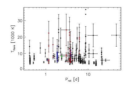
Figure 9: Flare temperature $\bar{T}_{\rm flare}(k)$ (as in top panel of Fig. 6) versus stellar rotation period. The horizontal error bars correspond to the uncertainty in the estimated rotation period, which is very small in most cases. Two flares with temperatures larger than 30,000 K have uncertainties around 10,000 K and their error bars are not shown for a better visualization. Stars identified as T Tauri are shown in red, and eclipsing binaries in blue, and their flare temperatures are connected by a dotted line of the same color. CoRoT 223983509 is shown in green as it has been classified as T Tauri and eclipsing binary. In the case of binaries, the period shown is their orbital period.

Table 2: The spectral type, rotation period, flare temperature, Gaia flare energy, and flare area for the 69 flaring stars analyzed. Their spectral type is given by the Exodat Database. Flares observed at different epochs (taken $\sim$4 years apart) are marked with a star next to their temperature. A small letter after the rotation period indicates: an eclipsing binary identified by Deleuil et al. (2018)^a, or by Klagyivik et al. (2017)^b, and a T Tauri analysed by Venuti et al. (2015)^t. The value in the $P_{\rm rot}$ column for eclipsing binaries is actually their orbital period. In the case of the eclipsing binary CoRoT 102615551, the value obtained by Deleuil et al. (2018) $-$ marked with the symbol ^† is given. Due to the large uncertainties, there are flares with the same temperature and uncertainty for some stars.

CoRoT ID	Type	Prot [d]	$T_{\rm flare}$ [1000 K]	$E_{G,f}$ [erg]	$A_{\rm flare}$ [cm2]
223941972	A0IV	4.90$\pm$0.02	8.84$\pm$0.83	(33.4$\pm$4.9)$\times 10^{34}$	(25.5$\pm$3.0)$\times 10^{19}$
224008170	A5IV	1.06$\pm$0.01	6.44$\pm$0.66	(92.6$\pm$6.6)$\times 10^{33}$	(25.7$\pm$1.2)$\times 10^{20}$
110685010	F0II	5.510$\pm$0.007	18.9$\pm$6.1	(54.1$\pm$9.5)$\times 10^{32}$	(57.6$\pm$4.4)$\times 10^{16}$
			19.6$\pm$6.4	(70.1$\pm$9.6)$\times 10^{32}$	(16.7$\pm$1.9)$\times 10^{17}$
102326330	F5III	4.141$\pm$0.001	8.2$\pm$1.4	(72.0$\pm$2.4)$\times 10^{33}$	(49.5$\pm$1.4)$\times 10^{19}$
			9.1$\pm$1.7	(88.5$\pm$2.5)$\times 10^{33}$	(45.1$\pm$1.2)$\times 10^{19}$
102332965	F5III	6.247$\pm$0.006	8.0$\pm$1.4	(12.7$\pm$1.4)$\times 10^{33}$	(20.1$\pm$2.1)$\times 10^{19}$
			17.2$\pm$5.6	(7.5$\pm$1.3)$\times 10^{33}$	(30.7$\pm$3.4)$\times 10^{18}$
102948867	F5III	8.79$\pm$0.01	9.3$\pm$1.8	(5.0$\pm$1.4)$\times 10^{32}$	(21.4$\pm$4.6)$\times 10^{18}$
			11.2$\pm$2.5	(6.0$\pm$1.5)$\times 10^{32}$	(5.4$\pm$1.0)$\times 10^{18}$
			11.2$\pm$2.5	(7.9$\pm$1.9)$\times 10^{32}$	(6.0$\pm$1.2)$\times 10^{18}$
			16.1$\pm$4.6	(11.3$\pm$1.1)$\times 10^{32}$	(37.2$\pm$2.7)$\times 10^{17}$
			16.6$\pm$4.9	(18.7$\pm$1.3)$\times 10^{32}$	(32.1$\pm$1.6)$\times 10^{17}$
			20.3$\pm$6.1	(43.7$\pm$8.5)$\times 10^{31}$	(11.8$\pm$1.1)$\times 10^{17}$
			33.8$\pm$9.5	(7.4$\pm$2.4)$\times 10^{32}$	(6.8$\pm$2.2)$\times 10^{17}$
			37$\pm$10	(17.2$\pm$5.7)$\times 10^{32}$	(7.8$\pm$2.5)$\times 10^{17}$
223940041	F5III	3.377$\pm$0.006	10.4$\pm$2.2	(70.9$\pm$2.7)$\times 10^{33}$	(32.7$\pm$1.0)$\times 10^{19}$
			13.6$\pm$3.5	(46.1$\pm$6.9)$\times 10^{32}$	(38.3$\pm$3.0)$\times 10^{18}$
223984608	F5III	6.20$\pm$0.02t	10.0$\pm$2.1	(63.8$\pm$2.3)$\times 10^{34}$	(226.9$\pm$7.4)$\times 10^{19}$
			18.8$\pm$7.1	(17.1$\pm$3.1)$\times 10^{33}$	(10.4$\pm$1.0)$\times 10^{19}$
			19.8$\pm$8.1∗	(15.7$\pm$2.2)$\times 10^{33}$	(11.1$\pm$1.1)$\times 10^{19}$
102925086	F8I	13$\pm$3	9.9$\pm$2.3	(87.0$\pm$8.2)$\times 10^{32}$	(109.6$\pm$6.3)$\times 10^{17}$
			21.0$\pm$7.0	(5.6$\pm$1.3)$\times 10^{33}$	(13.5$\pm$2.4)$\times 10^{17}$
110773079	F8I	5.29$\pm$0.05	6.19$\pm$0.95	(12.9$\pm$2.5)$\times 10^{33}$	(20.3$\pm$2.6)$\times 10^{19}$
			6.27$\pm$0.97	(32.8$\pm$8.2)$\times 10^{33}$	(16.4$\pm$2.4)$\times 10^{19}$
			9.1$\pm$1.9	(7.8$\pm$2.4)$\times 10^{34}$	(19.9$\pm$4.9)$\times 10^{19}$
			12.5$\pm$3.3	(37.3$\pm$6.9)$\times 10^{33}$	(26.6$\pm$3.6)$\times 10^{18}$
211607284	F8IV	2.013$\pm$0.001	7.7$\pm$1.1	(26.2$\pm$4.8)$\times 10^{31}$	(68.2$\pm$8.9)$\times 10^{17}$
			14.0$\pm$3.5	(20.2$\pm$6.3)$\times 10^{31}$	(13.1$\pm$3.1)$\times 10^{17}$
			14.4$\pm$3.7	(38.7$\pm$5.8)$\times 10^{31}$	(21.7$\pm$2.5)$\times 10^{17}$
			22.8$\pm$8.4	(5.4$\pm$1.5)$\times 10^{32}$	(13.6$\pm$3.4)$\times 10^{17}$
			24.5$\pm$9.2	(4.1$\pm$1.0)$\times 10^{32}$	( 9.9$\pm$2.1)$\times 10^{17}$
221628176	F8IV	3.43$\pm$0.03	6.71$\pm$0.88	(10.0$\pm$3.7)$\times 10^{34}$	(3.5$\pm$1.3)$\times 10^{21}$
223959652	F8IV	3.636$\pm$0.004t	6.19$\pm$0.70	(79.2$\pm$4.9)$\times 10^{33}$	(45.9$\pm$1.9)$\times 10^{20}$
			6.56$\pm$0.80	(18.5$\pm$1.3)$\times 10^{34}$	(28.5$\pm$1.3)$\times 10^{20}$
			6.62$\pm$0.81	(22.1$\pm$1.5)$\times 10^{34}$	(31.9$\pm$1.4)$\times 10^{20}$
			12.8$\pm$2.9	(30.1$\pm$7.8)$\times 10^{33}$	(7.9$\pm$1.6)$\times 10^{20}$
			21.2$\pm$8.0∗	(21.3$\pm$3.6)$\times 10^{33}$	(14.5$\pm$1.3)$\times 10^{19}$
			22.7$\pm$9.3∗	(18.3$\pm$4.4)$\times 10^{33}$	(13.9$\pm$1.5)$\times 10^{19}$
223970694	F8IV	1.478$\pm$0.002t	7.8$\pm$1.1	(22.7$\pm$1.4)$\times 10^{34}$	(29.8$\pm$1.4)$\times 10^{20}$
			15.4$\pm$4.1	(11.8$\pm$1.5)$\times 10^{34}$	(28.3$\pm$1.7)$\times 10^{19}$
223983509	G0III	2.383$\pm$0.003at	8.0$\pm$1.3	(25.1$\pm$2.1)$\times 10^{34}$	(168.9$\pm$8.5)$\times 10^{19}$
			8.5$\pm$1.4	(27.7$\pm$1.5)$\times 10^{34}$	(24.6$\pm$1.0)$\times 10^{20}$
102899501	G0III	1.6236$\pm$0.0004	8.3$\pm$1.3	(5.5$\pm$1.5)$\times 10^{34}$	(20.6$\pm$2.8)$\times 10^{19}$
104228454	G0III	13.69$\pm$0.02	4.57$\pm$0.54	(8.1$\pm$1.0)$\times 10^{35}$	( 97.0$\pm$7.7)$\times 10^{20}$
106054338	G0III	0.529$\pm$0.001	6.60$\pm$0.83	(149.4$\pm$8.4)$\times 10^{32}$	(39.5$\pm$1.3)$\times 10^{19}$
			7.10$\pm$0.95	(50.8$\pm$4.4)$\times 10^{32}$	(27.6$\pm$1.4)$\times 10^{19}$
			8.0$\pm$1.2	(48.5$\pm$4.5)$\times 10^{32}$	(156.1$\pm$8.2)$\times 10^{18}$
			8.6$\pm$1.4	(151.1$\pm$7.9)$\times 10^{32}$	(29.5$\pm$1.1)$\times 10^{19}$
102631863	G0III	47$\pm$11	21.1$\pm$6.8	(18.0$\pm$5.4)$\times 10^{35}$	(8.6$\pm$2.4)$\times 10^{21}$
102715243	G0IV	2.2460$\pm$0.0004	10.9$\pm$2.3	(41.9$\pm$4.3)$\times 10^{33}$	(80.8$\pm$6.8)$\times 10^{19}$
			19.4$\pm$6.1	(32.1$\pm$6.8)$\times 10^{33}$	(13.4$\pm$1.9)$\times 10^{19}$
102859855	G0IV	8.13$\pm$0.05	8.7$\pm$1.5	(64.9$\pm$8.8)$\times 10^{33}$	(67.4$\pm$6.6)$\times 10^{18}$
110744989	G0IV	0.413$\pm$0.001	8.7$\pm$1.5	(17.8$\pm$1.0)$\times 10^{33}$	(46.3$\pm$1.8)$\times 10^{19}$
			14.3$\pm$3.9	(10.4$\pm$1.1)$\times 10^{33}$	(58.3$\pm$3.7)$\times 10^{18}$
223980621	G0V	3.1$\pm$0.7t	8.5$\pm$1.3	(11.3$\pm$2.6)$\times 10^{34}$	(56.5$\pm$9.5)$\times 10^{19}$
			9.1$\pm$1.5	(25.8$\pm$3.0)$\times 10^{34}$	(19.9$\pm$2.1)$\times 10^{20}$
			24.3$\pm$9.5	(28.5$\pm$6.5)$\times 10^{33}$	(19.4$\pm$2.6)$\times 10^{19}$
105085606	G2I	5.248$\pm$0.007	8.7$\pm$1.7	(21.3$\pm$2.1)$\times 10^{32}$	(37.2$\pm$2.3)$\times 10^{18}$
			11.9$\pm$2.9∗	(8.4$\pm$1.5)$\times 10^{32}$	(70.3$\pm$6.3)$\times 10^{17}$
500007157	G2I	4.34$\pm$0.02t	5.99$\pm$0.92	(14.3$\pm$4.6)$\times 10^{34}$	(13.7$\pm$3.5)$\times 10^{20}$
223993277	G2IV	1.175$\pm$0.003t	4.23$\pm$0.41	(86.0$\pm$7.6)$\times 10^{33}$	(19.3$\pm$1.1)$\times 10^{21}$
			5.65$\pm$0.64	(42.6$\pm$1.7)$\times 10^{34}$	(84.3$\pm$3.3)$\times 10^{20}$
			6.02$\pm$0.73	(52.4$\pm$5.5)$\times 10^{34}$	(15.6$\pm$1.0)$\times 10^{21}$
			6.08$\pm$0.73∗	(13.9$\pm$1.0)$\times 10^{34}$	(69.5$\pm$3.5)$\times 10^{20}$
			14.5$\pm$3.7∗	(24.6$\pm$5.0)$\times 10^{33}$	(25.9$\pm$2.4)$\times 10^{19}$
			22.4$\pm$7.2∗	(21.0$\pm$3.7)$\times 10^{33}$	(11.1$\pm$1.4)$\times 10^{19}$
102854684	G2IV	1.097$\pm$0.003b	6.15$\pm$0.79	(48.6$\pm$1.7)$\times 10^{35}$	(46.5$\pm$1.7)$\times 10^{21}$
604183778	G2V	0.740$\pm$0.003	13.3$\pm$3.2	(24.1$\pm$4.4)$\times 10^{33}$	(41.8$\pm$4.5)$\times 10^{19}$
102926046	G2V	2.368$\pm$0.004	6.77$\pm$0.84	(164.2$\pm$7.8)$\times 10^{33}$	(239.8$\pm$8.2)$\times 10^{19}$
221649345	G2V	1.536$\pm$0.006	8.6$\pm$1.4	(70.3$\pm$5.0)$\times 10^{33}$	(75.8$\pm$3.1)$\times 10^{19}$
223945488	G2V	3.142$\pm$0.004	5.90$\pm$0.75	(24.6$\pm$2.8)$\times 10^{34}$	(135.7$\pm$8.2)$\times 10^{19}$
315258285	G2V	0.897$\pm$0.002	4.78$\pm$0.48	(10.4$\pm$1.2)$\times 10^{33}$	(119.0$\pm$7.4)$\times 10^{19}$
102632674	G5II	6.07$\pm$0.02	5.12$\pm$0.80	(13.5$\pm$3.3)$\times 10^{32}$	(19.2$\pm$2.5)$\times 10^{19}$
			6.3$\pm$1.1	(37.9$\pm$2.4)$\times 10^{32}$	(150.3$\pm$7.0)$\times 10^{18}$
			6.5$\pm$1.2	(38.3$\pm$2.5)$\times 10^{32}$	(149.8$\pm$6.7)$\times 10^{18}$
			6.6$\pm$1.2	(12.3$\pm$1.5)$\times 10^{32}$	(78.3$\pm$5.7)$\times 10^{18}$
			6.7$\pm$1.2	(16.9$\pm$5.2)$\times 10^{32}$	(10.8$\pm$2.1)$\times 10^{19}$
			7.0$\pm$1.3	(34.9$\pm$2.9)$\times 10^{32}$	(42.8$\pm$2.1)$\times 10^{18}$
			7.2$\pm$1.4	(29.2$\pm$1.8)$\times 10^{32}$	(61.6$\pm$2.7)$\times 10^{18}$
			7.2$\pm$1.4	(10.5$\pm$1.1)$\times 10^{32}$	(51.5$\pm$3.4)$\times 10^{18}$
			7.2$\pm$1.4	(45.7$\pm$2.4)$\times 10^{32}$	(68.7$\pm$2.5)$\times 10^{18}$
			7.7$\pm$1.5	(22.7$\pm$1.8)$\times 10^{32}$	(63.7$\pm$3.3)$\times 10^{18}$
			7.7$\pm$1.5	(20.0$\pm$2.2)$\times 10^{32}$	(48.6$\pm$3.6)$\times 10^{18}$
			8.4$\pm$1.8	(12.9$\pm$1.3)$\times 10^{32}$	(41.8$\pm$2.5)$\times 10^{18}$
			9.3$\pm$2.1	(17.0$\pm$3.0)$\times 10^{32}$	(23.1$\pm$1.2)$\times 10^{18}$
110680553	G5II	6.567$\pm$0.002	6.13$\pm$1.00	(37.1$\pm$5.4)$\times 10^{33}$	(89.6$\pm$7.0)$\times 10^{18}$
104150155	G5III	6.867$\pm$0.002	4.89$\pm$0.74	(61.0$\pm$9.3)$\times 10^{34}$	(57.1$\pm$5.6)$\times 10^{20}$
			5.15$\pm$0.80	(18.0$\pm$3.0)$\times 10^{34}$	(34.9$\pm$3.1)$\times 10^{20}$
102615551	G8III	3.8771$\pm$0.0004a†	6.16$\pm$0.91	(11.5$\pm$2.1)$\times 10^{32}$	(8.1$\pm$1.2)$\times 10^{19}$
			7.9$\pm$1.4	(33.6$\pm$5.2)$\times 10^{32}$	(37.1$\pm$5.2)$\times 10^{18}$
			8.7$\pm$1.8	(20.5$\pm$3.7)$\times 10^{32}$	(40.7$\pm$6.0)$\times 10^{18}$
			8.8$\pm$1.8	(16.6$\pm$2.6)$\times 10^{32}$	(39.9$\pm$5.6)$\times 10^{18}$
			9.7$\pm$2.1∗	(20.2$\pm$3.1)$\times 10^{32}$	(26.6$\pm$3.8)$\times 10^{18}$
			9.8$\pm$2.2∗	(14.1$\pm$2.5)$\times 10^{32}$	(35.1$\pm$5.7)$\times 10^{18}$
			11.1$\pm$2.8∗	(8.0$\pm$2.2)$\times 10^{32}$	(15.2$\pm$3.0)$\times 10^{18}$
			12.3$\pm$3.3∗	(12.9$\pm$8.7)$\times 10^{32}$	(2.3$\pm$1.1)$\times 10^{19}$
110662866	G8III	2.959$\pm$0.001	5.45$\pm$0.70	(19.6$\pm$4.2)$\times 10^{34}$	(13.8$\pm$2.2)$\times 10^{20}$
102590771	G8V	3.71$\pm$0.03	3.57$\pm$0.35	(9.6$\pm$1.6)$\times 10^{34}$	(8.7$\pm$1.2)$\times 10^{21}$
			4.88$\pm$0.54	(7.0$\pm$1.5)$\times 10^{34}$	(12.3$\pm$2.0)$\times 10^{20}$
			8.7$\pm$1.5	(3.5$\pm$1.5)$\times 10^{34}$	(12.8$\pm$5.0)$\times 10^{19}$
223961132	G8V	3.829$\pm$0.005t	4.59$\pm$0.58	(9.5$\pm$3.0)$\times 10^{35}$	(9.4$\pm$2.8)$\times 10^{22}$
			4.90$\pm$0.50	(60.4$\pm$8.6)$\times 10^{34}$	(17.7$\pm$2.2)$\times 10^{21}$
			5.75$\pm$0.65	(10.0$\pm$1.3)$\times 10^{35}$	(16.9$\pm$2.1)$\times 10^{21}$
			6.75$\pm$0.89	(44.7$\pm$5.8)$\times 10^{34}$	(74.8$\pm$9.3)$\times 10^{20}$
			7.9$\pm$1.4	(21.3$\pm$3.1)$\times 10^{34}$	(25.3$\pm$3.2)$\times 10^{20}$
			9.8$\pm$2.0∗	(4.9$\pm$1.2)$\times 10^{34}$	(12.5$\pm$2.3)$\times 10^{20}$
			11.3$\pm$2.6∗	(4.2$\pm$1.3)$\times 10^{34}$	(10.6$\pm$2.6)$\times 10^{20}$
			17.2$\pm$6.2∗	(45.9$\pm$8.2)$\times 10^{33}$	(33.1$\pm$4.8)$\times 10^{19}$
110681935	K0III	4.33$\pm$0.10	7.1$\pm$1.1	(5.5$\pm$1.9)$\times 10^{34}$	(4.2$\pm$1.2)$\times 10^{20}$
			7.3$\pm$1.2	(30.8$\pm$7.3)$\times 10^{33}$	(11.1$\pm$1.5)$\times 10^{19}$
			13.1$\pm$3.6	(3.6$\pm$1.3)$\times 10^{34}$	(4.0$\pm$1.3)$\times 10^{19}$
110747714	K0III	4.775$\pm$0.006	5.71$\pm$0.75	(18.5$\pm$5.5)$\times 10^{34}$	(13.8$\pm$3.5)$\times 10^{20}$
			6.51$\pm$0.94	(7.9$\pm$1.1)$\times 10^{34}$	(33.0$\pm$2.4)$\times 10^{19}$
221647275	K0III	3.732$\pm$0.001	5.11$\pm$0.66	(34.5$\pm$3.3)$\times 10^{32}$	(52.6$\pm$3.6)$\times 10^{19}$
			5.69$\pm$0.77	(30.0$\pm$1.8)$\times 10^{32}$	(21.9$\pm$1.1)$\times 10^{19}$
			7.3$\pm$1.2	(35.9$\pm$1.6)$\times 10^{32}$	(72.6$\pm$2.4)$\times 10^{18}$
			8.2$\pm$1.4	(29.9$\pm$3.0)$\times 10^{32}$	(59.4$\pm$3.0)$\times 10^{18}$
102718810	K0III	1.86$\pm$0.03b	4.93$\pm$0.61	(42.1$\pm$4.4)$\times 10^{32}$	(88.0$\pm$5.4)$\times 10^{19}$
			5.86$\pm$0.79	(31.4$\pm$1.5)$\times 10^{33}$	(81.6$\pm$3.1)$\times 10^{19}$
			6.9$\pm$1.1	(26.8$\pm$1.2)$\times 10^{33}$	(43.5$\pm$1.2)$\times 10^{19}$
			7.5$\pm$1.2	(60.4$\pm$4.1)$\times 10^{32}$	(21.2$\pm$1.0)$\times 10^{19}$
			8.0$\pm$1.3	(40.6$\pm$7.1)$\times 10^{32}$	(17.9$\pm$2.4)$\times 10^{19}$
			8.3$\pm$1.4	(28.9$\pm$4.2)$\times 10^{32}$	(25.4$\pm$2.9)$\times 10^{19}$
			8.4$\pm$1.5	(157.6$\pm$9.5)$\times 10^{32}$	(206.1$\pm$7.6)$\times 10^{18}$
			8.7$\pm$1.5	(44.4$\pm$2.0)$\times 10^{33}$	(281.8$\pm$9.4)$\times 10^{18}$
			8.9$\pm$1.6	(101.1$\pm$7.1)$\times 10^{32}$	(18.8$\pm$1.0)$\times 10^{19}$
			9.1$\pm$1.7	(43.6$\pm$7.0)$\times 10^{32}$	(14.4$\pm$1.0)$\times 10^{19}$
			9.5$\pm$1.8	(154.9$\pm$9.3)$\times 10^{32}$	(120.5$\pm$4.0)$\times 10^{18}$
			10.0$\pm$2.0	(109.1$\pm$6.8)$\times 10^{32}$	(81.2$\pm$3.6)$\times 10^{18}$
			10.6$\pm$2.3	(109.4$\pm$8.8)$\times 10^{32}$	(82.4$\pm$3.7)$\times 10^{18}$
			10.9$\pm$2.4	(76.8$\pm$7.0)$\times 10^{32}$	(107.9$\pm$6.2)$\times 10^{18}$
			14.6$\pm$3.9	(5.3$\pm$2.2)$\times 10^{33}$	(34.6$\pm$5.4)$\times 10^{18}$
223968260	K0V	1.645$\pm$0.001	5.26$\pm$0.70	(11.7$\pm$3.5)$\times 10^{34}$	(18.3$\pm$3.1)$\times 10^{20}$
110660270	K0V	1.969$\pm$0.001	5.77$\pm$0.74	(32.1$\pm$2.7)$\times 10^{34}$	(110.9$\pm$8.3)$\times 10^{20}$
110757572	K0V	6.676$\pm$0.002	4.60$\pm$0.51	(223.2$\pm$9.1)$\times 10^{32}$	(35.7$\pm$1.2)$\times 10^{20}$
			4.70$\pm$0.53	(24.1$\pm$1.4)$\times 10^{33}$	(35.2$\pm$1.3)$\times 10^{20}$
			4.77$\pm$0.54	(101.5$\pm$7.5)$\times 10^{32}$	(167.2$\pm$7.5)$\times 10^{19}$
			5.12$\pm$0.60	(114.8$\pm$8.6)$\times 10^{32}$	(152.9$\pm$6.9)$\times 10^{19}$
			5.42$\pm$0.65	(36.1$\pm$2.2)$\times 10^{33}$	(188.3$\pm$7.1)$\times 10^{19}$
			5.87$\pm$0.75	(27.0$\pm$2.2)$\times 10^{33}$	(73.4$\pm$3.8)$\times 10^{19}$
			6.86$\pm$0.99	(31.3$\pm$1.6)$\times 10^{33}$	(45.3$\pm$1.6)$\times 10^{19}$
			7.0$\pm$1.0	(21.4$\pm$1.3)$\times 10^{33}$	(82.6$\pm$3.9)$\times 10^{19}$
			7.9$\pm$1.3	(17.1$\pm$1.7)$\times 10^{33}$	(28.8$\pm$1.4)$\times 10^{19}$
211607099	K0V	0.974$\pm$0.001	10.3$\pm$2.3	(4.8$\pm$1.1)$\times 10^{34}$	(7.4$\pm$1.0)$\times 10^{19}$
101282630	K1III	13.866$\pm$0.004	4.15$\pm$0.48	(95.8$\pm$9.5)$\times 10^{34}$	(27.2$\pm$1.9)$\times 10^{21}$
			4.41$\pm$0.52	(137.2$\pm$9.2)$\times 10^{34}$	(41.0$\pm$2.5)$\times 10^{21}$
104939145	K1III	26$\pm$6	5.96$\pm$0.77	(28.6$\pm$4.8)$\times 10^{34}$	(52.9$\pm$8.1)$\times 10^{21}$
110661118	K1III	4.024$\pm$0.002	5.02$\pm$0.59	(5.7$\pm$1.9)$\times 10^{34}$	(8.3$\pm$1.3)$\times 10^{20}$
223988965	K1III	3.4$\pm$0.5t	5.18$\pm$0.73	(10.9$\pm$6.8)$\times 10^{35}$	(7.0$\pm$4.3)$\times 10^{21}$
101309841	K2III	8.587$\pm$0.007	4.42$\pm$0.62	(11.7$\pm$1.3)$\times 10^{35}$	(76.1$\pm$4.9)$\times 10^{20}$
			4.87$\pm$0.73	(94.0$\pm$8.8)$\times 10^{34}$	(44.3$\pm$2.4)$\times 10^{20}$
			12.6$\pm$3.6	(45.9$\pm$3.7)$\times 10^{34}$	(16.0$\pm$1.0)$\times 10^{19}$
105271299	K2III	10.48$\pm$0.03	3.93$\pm$0.52	(14.1$\pm$2.5)$\times 10^{34}$	(71.9$\pm$7.2)$\times 10^{20}$
			5.07$\pm$0.75	(20.5$\pm$6.8)$\times 10^{34}$	(4.9$\pm$1.4)$\times 10^{21}$
110669882	K2III	8.052$\pm$0.003	4.58$\pm$0.66	(102.0$\pm$9.3)$\times 10^{34}$	(15.3$\pm$1.0)$\times 10^{21}$
			4.68$\pm$0.68	(78.8$\pm$7.2)$\times 10^{34}$	(110.9$\pm$6.9)$\times 10^{20}$
			6.0$\pm$1.0	(110.0$\pm$5.7)$\times 10^{34}$	(79.2$\pm$3.4)$\times 10^{20}$
110741064	K2III	—	6.7$\pm$1.2	(40.0$\pm$3.6)$\times 10^{32}$	(36.8$\pm$2.1)$\times 10^{19}$
110752597	K2III	4.216$\pm$0.002	4.05$\pm$0.57	(42.5$\pm$8.7)$\times 10^{33}$	(11.5$\pm$1.1)$\times 10^{20}$
105132247	K2V	4.75$\pm$0.05	7.1$\pm$1.3	(4.9$\pm$1.3)$\times 10^{34}$	(39.0$\pm$4.0)$\times 10^{20}$
211644521	K2V	4.25$\pm$0.02	5.43$\pm$0.84	(10.9$\pm$1.1)$\times 10^{33}$	( 96.9$\pm$6.3)$\times 10^{19}$
105628093	K2V	0.5073$\pm$0.0008	4.38$\pm$0.59	(9.3$\pm$1.5)$\times 10^{33}$	(24.6$\pm$3.3)$\times 10^{20}$
300002990	K2V	6.56$\pm$0.03	4.63$\pm$0.66	(49.3$\pm$8.2)$\times 10^{33}$	(22.5$\pm$2.6)$\times 10^{20}$
			4.70$\pm$0.67	(12.8$\pm$1.2)$\times 10^{34}$	(119.8$\pm$6.8)$\times 10^{19}$
			5.23$\pm$0.79	(5.4$\pm$1.1)$\times 10^{34}$	(91.5$\pm$7.9)$\times 10^{19}$
			6.7$\pm$1.2	(9.4$\pm$1.5)$\times 10^{34}$	(36.5$\pm$3.7)$\times 10^{19}$
			8.0$\pm$1.6	(14.6$\pm$1.2)$\times 10^{34}$	(174.9$\pm$9.1)$\times 10^{18}$
500007248	K3I	3.78$\pm$0.02t	5.57$\pm$0.85	(32.4$\pm$7.6)$\times 10^{33}$	(51.8$\pm$8.0)$\times 10^{19}$
102646977	K3II	20.8$\pm$0.3	9.5$\pm$2.1	(4.4$\pm$1.0)$\times 10^{35}$	(12.5$\pm$1.9)$\times 10^{21}$
			10.5$\pm$2.5	(27.5$\pm$5.4)$\times 10^{34}$	(9.5$\pm$1.5)$\times 10^{21}$
			10.8$\pm$2.7	(36.4$\pm$7.1)$\times 10^{34}$	(7.4$\pm$1.2)$\times 10^{21}$
500007323	K3II	6$\pm$1	7.2$\pm$1.4	(22.0$\pm$2.4)$\times 10^{34}$	(15.1$\pm$1.4)$\times 10^{19}$
102379742	K3III	0.4231$\pm$0.0008	3.90$\pm$0.51	(1.7$\pm$1.1)$\times 10^{32}$	(5.5$\pm$3.8)$\times 10^{19}$
			4.27$\pm$0.57	(5.2$\pm$3.6)$\times 10^{33}$	(11.8$\pm$8.1)$\times 10^{20}$
			4.96$\pm$0.71	(2.2$\pm$1.6)$\times 10^{33}$	(5.2$\pm$3.6)$\times 10^{20}$
			5.11$\pm$0.74	(2.1$\pm$1.4)$\times 10^{34}$	(12.5$\pm$8.6)$\times 10^{20}$
			5.18$\pm$0.76	(10.8$\pm$7.4)$\times 10^{33}$	(8.8$\pm$6.0)$\times 10^{20}$
			5.33$\pm$0.79	(8.8$\pm$6.4)$\times 10^{33}$	(8.0$\pm$5.6)$\times 10^{20}$
			5.72$\pm$0.88	(5.2$\pm$3.6)$\times 10^{33}$	(3.2$\pm$2.2)$\times 10^{20}$
			5.76$\pm$0.89	(7.2$\pm$5.1)$\times 10^{33}$	(6.1$\pm$4.3)$\times 10^{20}$
			5.89$\pm$0.93	(8.0$\pm$5.5)$\times 10^{33}$	(5.9$\pm$4.0)$\times 10^{20}$
			6.2$\pm$1.0	(6.6$\pm$4.5)$\times 10^{33}$	(3.3$\pm$2.3)$\times 10^{20}$
			6.4$\pm$1.1	(2.4$\pm$1.7)$\times 10^{33}$	(2.5$\pm$1.7)$\times 10^{20}$
			6.6$\pm$1.1	(9.5$\pm$6.6)$\times 10^{33}$	(2.2$\pm$1.5)$\times 10^{20}$
			6.6$\pm$1.1	(12.8$\pm$8.8)$\times 10^{33}$	(3.3$\pm$2.2)$\times 10^{20}$
			7.1$\pm$1.3	(4.1$\pm$3.1)$\times 10^{33}$	(12.9$\pm$9.0)$\times 10^{19}$
			7.3$\pm$1.3	(12.5$\pm$8.9)$\times 10^{32}$	(1.7$\pm$1.2)$\times 10^{20}$
102646279	K3III	10.52$\pm$0.04	10.2$\pm$2.6	(15.5$\pm$1.7)$\times 10^{35}$	(20.0$\pm$1.6)$\times 10^{21}$
			12.1$\pm$3.6∗	(9.3$\pm$1.2)$\times 10^{35}$	(12.5$\pm$1.1)$\times 10^{21}$
102691871	K3III	7.138$\pm$0.004	5.9$\pm$1.0	(23.1$\pm$2.0)$\times 10^{35}$	(91.4$\pm$6.3)$\times 10^{20}$
101562259	K5III	7.4867$\pm$0.0008	4.43$\pm$0.77	(133.7$\pm$9.5)$\times 10^{33}$	(94.8$\pm$5.0)$\times 10^{20}$
			4.75$\pm$0.85	(42.0$\pm$3.2)$\times 10^{33}$	(36.9$\pm$1.9)$\times 10^{20}$
			4.84$\pm$0.87	(37.4$\pm$1.3)$\times 10^{34}$	(151.2$\pm$5.6)$\times 10^{20}$
			5.6$\pm$1.1	(54.5$\pm$4.9)$\times 10^{33}$	(21.1$\pm$1.1)$\times 10^{20}$
			6.5$\pm$1.4	(14.7$\pm$3.4)$\times 10^{33}$	(13.7$\pm$1.5)$\times 10^{20}$
102602133	K5III	21.3$\pm$0.1	3.70$\pm$0.62	(93.1$\pm$7.1)$\times 10^{35}$	(17.5$\pm$1.1)$\times 10^{22}$
			5.5$\pm$1.2∗	(24.3$\pm$4.4)$\times 10^{34}$	(11.0$\pm$1.7)$\times 10^{22}$
			5.8$\pm$1.3∗	(36.0$\pm$5.2)$\times 10^{34}$	(55.7$\pm$6.5)$\times 10^{21}$
			6.5$\pm$1.7∗	(44.7$\pm$7.2)$\times 10^{34}$	(35.7$\pm$4.4)$\times 10^{21}$
106048015	K5III	15.430$\pm$0.009	3.19$\pm$0.61	(22.5$\pm$3.9)$\times 10^{34}$	(29.8$\pm$2.5)$\times 10^{21}$
			3.35$\pm$0.65	(15.9$\pm$5.6)$\times 10^{34}$	(4.0$\pm$1.2)$\times 10^{22}$
			3.41$\pm$0.67	(13.1$\pm$2.8)$\times 10^{34}$	(16.5$\pm$2.3)$\times 10^{21}$
			3.53$\pm$0.70	(10.2$\pm$1.8)$\times 10^{34}$	(17.8$\pm$1.9)$\times 10^{21}$
			3.77$\pm$0.77	(20.3$\pm$2.7)$\times 10^{34}$	(17.2$\pm$2.0)$\times 10^{21}$
			4.20$\pm$0.90	(24.1$\pm$2.9)$\times 10^{34}$	(66.6$\pm$6.4)$\times 10^{20}$
			4.33$\pm$0.95	(34.3$\pm$4.9)$\times 10^{34}$	(84.3$\pm$7.8)$\times 10^{20}$
			4.6$\pm$1.0	(15.1$\pm$2.4)$\times 10^{34}$	(27.2$\pm$2.9)$\times 10^{20}$
			5.0$\pm$1.2	(65.7$\pm$8.8)$\times 10^{34}$	(42.1$\pm$4.2)$\times 10^{20}$

6 Calibration

The accuracy of Gaia photometry is better than any other major catalog currently available, even more with the improvements from Gaia Early Data Release 3 - Gaia EDR3 (Riello et al., 2021). We used the fact that the GAIA G band is very similar to the CoRoT White channel (see, for example, Fig.1 in Nèmec et al., 2020) to calibrate the analyzed flare flux.

Firstly, we searched the Gaia EDR3 for stars at the same coordinates ($\alpha$, $\delta$) as ours. We compared their coordinates differences and iteratively removed outliers. We ended up with a standard deviation of 0.15 arcsec in $\alpha$ and $\delta$. We selected only stars of Gaia that differ by less than 0.6 arcsec (4$\sigma$) in $\alpha$ and $\delta$ and its angular distance is less than 0.7 arcsec from the CoRoT coordinates, we found 66 out of 69 stars. The stars observed by Gaia that are closer to the three missing ones (CoRoT 102948867, 110685010 and 221647275) are 1.3, 2.1, and 2.7 arcsec away, respectively. Table 3 shows the corresponding Gaia ID EDR3. In Figure 10, we plotted GAIA G-band mean apparent magnitude (phot$\_$g$\_$mean$\_$mag), which is computed from the G-band mean flux applying the magnitude zero-point in the Vega scale, in the VEGAMAG photometric system (equation 1 in Andrae et al., 2018) versus the CoRoT magnitude in the White channel given by: -2.5 log₁₀ F_white. The CoRoT flux is in electrons per 32 s (Chaintreuil et al., 2016). After fitting a straight line to 66 stars and removing outliers from the residuals larger than 4$\sigma$ (empty blue circles), we fitted again a straight line through the selected full circles (corresponding to 64 stars) and obtained:

$$G=c_{0}+c_{1}\cdot m_{\rm CoRoT}$$ (12)

where $c_{0}$ = (27.6$\pm$0.3) mag and $c_{1}$ = 1.05$\pm$0.02. The two discarded outliers, CoRoT 500007248 and 500007323, are fainter than expected in the White channel, which may be due to an observational artifact or misidentification due to field contamination. Each of these stars contributes with only one flare in our analysis. There are eight stars in our set that have been observed twice (in 2008 and 2012). Their two CoRoT magnitudes are connected with a red horizontal line in Figure 10. The flare peak flux, $a_{0}$, observed in the White channel (Eq. 3) can be converted to GAIA G-band magnitude using Eq. 12:

$$G_{p}=c_{0}-2.5c_{1}\log_{10}(a_{0})$$ (13)

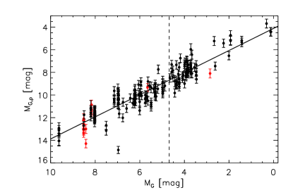
Figure 11: Absolute magnitude of the flare peak as a function of absolute stellar magnitude. Red dots correspond to flares in stars with an unreliable match to a star in the Gaia EDR3 catalog (i.e., empty circles in Fig. 10) and were not used in the fitting (full line). The vertical line shows the solar absolute magnitude estimated for the G band, $M_{G,\odot}$=4.68 mag (Andrae et al., 2018).

The uncertainty in estimating the G-band flare peak was obtained using standard error propagation. There is no perceptible dependence of the G-band flare peak, $G_{p}$, on the stellar magnitude, $G$. Using Eq. 12, the average apparent stellar magnitude of our 69 stars and its standard deviation are equal to G = (13.6$\pm$0.8) mag. However, their distances, $d$, range from 37 pc to 6.2 kpc. These stars are all in the galactic disk, as the CoRoT observations were in an area toward the Galactic center and another at the Galactic anticenter. We calculated the absolute stellar magnitude $M_{G}=G-5\log_{10}d+5$ and similarly the absolute magnitude of the flare peak, $M_{G,p}$, without taking the extinction into account. The flare peak amplitudes are in the range of $4\,<\,M_{G,p}\,<\,14$ mag. There is a good correlation between them (Figure 11). Fitting a straight line, we obtained:

$$M_{G,p}=(4.12\pm 0.09)+(0.98\pm 0.01)M_{G}$$ (14)

For a linear coefficient equal to 1, we have that the peak flare flux is $\sim$2.5% of the stellar flux in the Gaia G band.

Table 3: EDR3 Gaia identification used for each analyzed CoRoT star. The EDR3 Gaia observation corresponding to CoRoT 102379742 does not have an estimated parallax, and has been replaced by Gaia DR2 (labeled ‘R2’). The three EDR3 Gaia observations that are more than one arcsec away from the CoRoT target are marked with a $d$ and the two that are fainter than expected are indicated by an $F$.

CoRoT ID	Gaia ID	CoRoT ID	Gaia ID	CoRoT ID	Gaia ID
101282630	4263419769100038016	104228454	4479364776186624640	211644521	4269234708175942784
101309841	4287737908286241408	104939145	4284794275144637824	221628176	3323880005037073280
101562259	4287508488312311168	105085606	4283813132812345856	221647275	3324510948616275200d
102326330	3317450576432937984	105132247	4284031866916578688	221649345	3323856709134836480
102332965	3318597019166336896	105271299	4286729793567044352	223940041	3326099953372611968
102379742	3317374843273655040R2	105628093	4285482809953521920	223941972	3326973098749988736
102590771	3107330708913023488	106048015	4285502772956212480	223945488	3133881406461641088
102602133	3119470622952565504	106054338	4285618908854461184	223959652	3326704852270253056
102615551	3119353524964187520	110660270	3101935229255761408	223961132	3326895724912475648
102631863	3107228694850611968	110661118	3102183104708835328	223968260	3133861271655267072
102632674	3125806455627199104	110662866	3101991922824716416	223970694	3326703512240456064
102646279	3107323179828911104	110669882	3102084560979475840	223980621	3326929427518677504
102646977	3107338577293220480	110680553	3102338273286874240	223983509	3326931699558507648
102691871	3119514878295078144	110681935	3101134647354726272	223984608	3326685443313414144
102715243	3107267791930670976	110685010	3101901526654756864d	223988965	3326697984617869824
102718810	3107362079353715584	110741064	3102360362299563520	223993277	3326722276952860672
102854684	3106096674609281920	110744989	3101876478405414016	224008170	3326640844372957824
102859855	3106107330427498752	110747714	3101862833286509568	300002990	3102196814244084352
102899501	3106093827050203520	110752597	3102390912405546880	315258285	3120331437476706688
102925086	3106193569071435264	110757572	3101907569665841536	500007157	3326739903498311808
102926046	3106292422038384384	110773079	3102022880948173056	500007248	3326739869138571776F
102948867	3105880590514179456d	211607099	4280865410836745984	500007323	3326895342663197056F
104150155	4478967135257757056	211607284	4268382891546982528	604183778	3322004650516148992

The Gaia flare energy, $E_{G,f}$, was calculated by multiplying the flare equivalent duration ED (Eq. 4) observed in the White channel, measured in units of time, by the stellar luminosity in the Gaia bandpass filter:

$$E_{G,f}={\rm ED}_{\rm White}\cdot L_{G}$$ (15)

As the flare equivalent duration varies with the observed bandpass filter by two or more orders of magnitude (Hawley et al., 2014), we did not attempt to estimate the bolometric energy. To calculate the stellar luminosity in Gaia’s G-band, $L_{G}$, we first converted mean flux $f_{G}$ (phot$\_$g$\_$mean$\_$flux [$e^{-}s^{-1}$]) into mean energy [W m^-2 nm^-1] by multiplying it by $c_{\lambda}$ = 1.346109 $\times 10^{-21}$ as described in the Gaia photometric calibration (Montegriffo, 2021). Then we multiplied the stellar energy by 4$\pi d^{2}$ and by Gaia filter FWHM, $\Gamma_{G}$, to obtain $L_{G}$ (as in Hawley et al., 2014):

$$L_{G}=f_{G}\cdot c_{\lambda}\cdot 4\pi d^{2}\cdot\Gamma_{G}$$ (16)

where $\Gamma_{G}$ = 454.82 nm (Table 3 in Riello et al., 2021). The observed flare energies are in the range $10^{32}\,<\,E_{G,f}\,<\,10^{37}$ erg, and are given in Table 2. The energy of sixteen flares observed at five stars, for which we did not find a good match with Gaia observations (labeled in Table 3), was not used in our analysis, and their values in the table should be used with caution. Fitting a straight line to the logarithm of the flare energy as a function of the logarithm of the stellar luminosity, we get:

$$E_{G,f}=(4\pm 1)\times 10^{-6}\,L_{G}^{(1.218\pm 0.005)}$$ (17)

where $E_{G,f}$ and $L_{G}$ are in erg and erg s^-1 respectively. Flare energy exponentially increases with stellar luminosity. As in Fig. 6 (2nd row), the top panel in Figure 12 shows the flare energy in intervals of half-spectral type of its star, where the energies are in ascending order inside each range. The weighted average of the flare energy over each interval is in the bottom panel. The dashed (dotted) line indicates the weighted (unweighted) average of the mean energy including all stellar luminosity classes (black circles). There is some weak indication of a possible increase of flare energy for late-type stars.

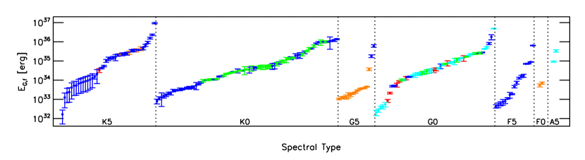
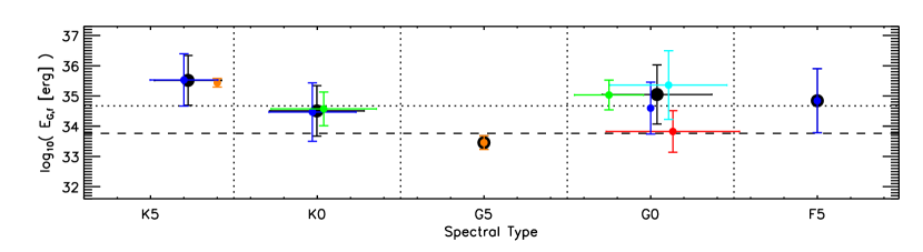
Figure 12: Top panel. Gaia flare energy as function of spectral type, going from late to early type stars, in intervals of half a spectral class. The spectral type at the center of each interval is indicated at the bottom of the plot. The flare energies are in ascending order inside each interval. The different colors represent the different luminosity classes, as in Fig. 6, where classes I to V are in red, orange, blue, cyan and, green respectively. Bottom panel. Weighted average of the flare energy as a function of the average spectral subclass corresponding to the flares within each interval of half a spectral class shown in the top panel. The averages for a given luminosity class, when there are 4 or more flares, are shown in different colors (as in the top panel). The averages including all luminosity classes are shown in black. The vertical error bars correspond to the standard deviation of the flare energy weighted average and the horizontal error bars to the standard deviation of the average of the spectral subclass. The absence of a horizontal bar means that only one spectral type was used in the energy averaged.

Howard et al. (2020) reported a weak correlation between the flare temperature, integrated over the entire flare, and flare energy in the g’ band. We do not see any indication of a dependence between our estimation of flare energy in the Gaia G band and flare temperature. Furthermore, we do not see a variation of the flare energy with the stellar rotation (Fig. 9). We looked for a complex dependence using the theoretical estimate by Namekata et al. (2017) of the bolometric flare energy:

$$E_{\rm bol}=c\,d^{3}B^{5}$$ (18)

where $c=5.8\times 10^{19}$ erg min^-3 G^-5. In addition to the implication that a flare with a longer duration ($d$) will have higher energy, they also deduced, considering the dependence of the Alfvén velocity on the magnetic field, that a stronger local magnetic field $B$ will imply a flare with larger energy. It is expected that greater amounts of magnetic energy stored, for example, at large spots, lead to more energetic flares (e.g. Candelaresi et al., 2014). The coefficient $c$ was estimated from the average values of their solar flare observations, which are: $d$ = 3.5 minutes, $E_{bol}$ = 1.5 $\times 10^{30}$ erg, and $B$= 57 G.

Figure 13 shows the flare energy in the Gaia band versus the flare duration given by the e-folding rise time plus the e-folding decay time observed by CoRoT. In the top panel, the different colors correspond to four different stellar rotation ranges and, in the bottom panel, they correspond to three different flare temperature intervals. Similarly to the relation given by Eq. 18, the panels show, for various values of $B$, the following relationship: $E_{G,f}=c^{\prime}d_{r+d}^{3}B^{5}$ where $c^{\prime}$ = 3.7 $\times 10^{18}$ erg min^-3 G^-5. To obtain $c^{\prime}$, we arbitrarily increased the flare duration value by 25% to account for the flare rising phase (not included before) and divided their bolometric energy estimate by 8 to adjust for the flare energy in the Gaia G band. This factor was roughly estimated using the relation in Eq. 15, where we assumed that the flare duration in the Gaia passband is the same as that at all wavelengths, we used the GAIA DR2 estimate of stellar luminosity (‘lum$\_$val’), and we extrapolated to the low value of the average solar flare energy. Namekata et al. (2017) also used the duration of the flare observed in visible light (more specifically, in the SDO/HMI’s narrow passband around the Fe I 6173.3Å  line) to estimate the flare bolometric energy. Since the $c^{\prime}$ coefficient was not precisely determined, all straight lines in Fig. 13 might be horizontally displaced by a small amount. We can see in the upper panel that flares observed in fast rotators, $P_{\rm rot}<$1 d (blue circles), are associated with magnetic fields slightly larger than $\sim$200 G, while slower rotators, $7\leq P_{\rm rot}<$20 d (red circles), are mostly associated with B slightly smaller than $\sim$200G. Interestingly, flares in stars with longer rotation periods, $P_{\rm rot}>$20 d (black circles), unexpectedly correspond to large magnetic fields ($B\gtrsim$800 G). These nine flares were observed on 4 stars (CoRoT 102602133, 102631863, 104939145, and 102646977), none of which were identified as an eclipsing binary star or a T Tauri star. Four of these flares were observed on CoRoT 102602133, but only one corresponds to a lower magnetic field as expected (B$\lesssim$200 G). This flare also differs from the others for having a much longer duration and a low temperature: $T_{\rm flare}$ = (3700$\pm$600) K. One of the flares on a star with $P_{\rm rot}>$20 d (black circles) has a very high temperature: $T_{\rm flare}$=(21100$\pm$6800) K (the one with $E_{G,f}$ = 1.8 $\times 10^{36}$ erg in the Figure) in contrast to the low temperature just mentioned. The bottom panel shows the variation with the flare temperature, where we see no clear interrelationship. We note, however, that flares with $T_{\rm flare}<$5,000 K (black symbols) correspond to $B\lesssim$ 400 G. In addition, most high-temperature flares ($\gtrsim$ 14,000 K) are short-lived (less than 10 minutes). For 40% of flares that last less than 10 minutes, the ascending phase is longer than the descending phase (i.e., $a_{2}<a_{3}$ in Equation 3). These flares correspond to 12% of the analyzed flares, and all but two have a duration smaller than 10 minutes.

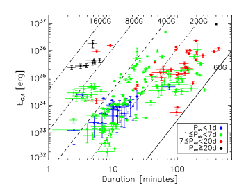
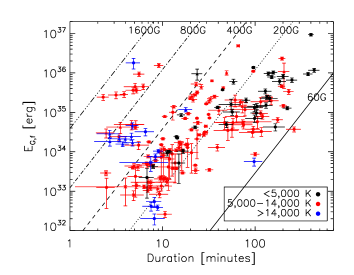
Figure 13: Gaia flare energy $E_{G,f}$ versus flare duration $d_{r+d}$. The black lines correspond to: $E_{G,f}=c^{\prime}d_{r+d}^{3}B^{5}$ for different B values (see text). The different colors stand for different intervals of stellar rotation in the top panel and for different intervals of flare temperature in the bottom panel. Eclipsing binaries are shown by stars and T Tauris by triangles.

We estimated the area of the flares, $A_{\rm flare}$, observed by the CoRoT White channel using Eq. 8 in units of energy, where the stellar luminosity, $L_{G}$, is given by Eq. 16. The flare area varies by 5 orders of magnitude, from $10^{18}$ to $10^{23}$ cm², i.e., 30 $\mu$sh to 3 sh (solar hemisphere), and is displayed in Table 2. The area uncertainty was estimated by propagating the errors of ED, duration, $L_{G}$, and flare surface brightness. Figure 14 (top panel) shows the variation of flare area with flare energy. The flare area increases (almost linearly) with flare energy: $\log_{10}A_{\rm flare}=-(7.87\pm 0.09)+(0.830\pm 0.002)\log_{10}E_{G,f}$, in cgs units (shown as red line in the top panel), This is expected (Eq. 8 and 15), as well as that the flare area is proportional to $L_{G}^{(1.144\pm 0.003)}$. The stellar luminosity is proportional to its surface area, for a given effective temperature, therefore, in principle, the area of the flare is increasing with the area of the star. However, we do not observe any clear dependence of flare area with spectral type or luminosity class in our data. Figure 14 (middle panel) shows the variation of flare area with flare temperature. For $T_{\rm flare}\lesssim$ 7,500 K, the flare area decreases, in most cases, as temperature increases. Analyzing the flare energy-to-area ratio versus temperature (Fig. 14 bottom panel), we did a log-log fit and obtained that the ratio, in cgs units, is proportional to T${}_{\rm flare}^{(2.35\pm 0.03)}$ (red dashed line). It seems that there is a change in behavior where, for flares with T${}_{\rm flare}>$ 10,000 K, the ratio seems to be constant, its weighted average is equal to E_G,f/A${}_{\rm flare}=1.7\times 10^{14}$ erg cm^-2 (horizontal dotted blue line). Fitting again now only for $T_{\rm flare}<$ 10,000 K, we obtain: E_G,f/$A_{\rm flare}\propto$ T${}_{\rm flare}^{(2.60\pm 0.04)}$ (red full line). As the temperature percentage uncertainties increase with temperature and the number of flares decreases, this possible saturation at T${}_{\rm flare}\gtrsim$ 10,000 K should be regarded with caution.

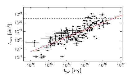
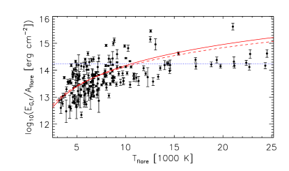
Figure 14: Flare area versus flare energy (top) and flare temperature (middle). The horizontal dashed line corresponds to the area of one solar hemisphere. The red line in the top panel shows the linear fit to the data. The bottom panel shows the flare energy divided by flare area, in cgs units, versus flare temperature. The red dashed line shows the fit to all points. The full red line shows a fit to flares with $T_{\rm flare}<$ 10,000 K. The blue dotted horizontal line is the weighted mean for flares with $T_{\rm flare}>$ 10,000 K. The flare temperature uncertainties were omitted in the middle and bottom panel for a better visualization.

7 Conclusions

Assuming that the spectrum of white-light flares can be described by blackbody radiation, we determined the effective flare temperature for more than 200 flares observed by CoRoT in 69 F, G, and K-type stars. The temperatures were obtained using the flare equivalent duration and stellar flux observed in the Blue and Red channels. The wavelength limits for the color channels were estimated using stellar spectra from the Pickles library for the spectral type and luminosity class of the star given by the Exodat Database. We took the uncertainties in the stellar classification into account and carefully propagated them in our estimate of the flare temperature.

The estimated flare temperatures vary from 3,000 K up to 30,000 K. Its uncertainties steadily increase from 10% at 3,000 K to about 40% at 25,000 K, as the blackbody radiation maximum moves toward UV wavelengths and out of the CoRoT Response Function. The expected value of the temperature distribution of the 209 analyzed flares is equal to 6,400 K with a standard deviation of 2,800 K. These flares have been observed in A5$-$K5 stars. The mean spectral type, weighted by the number of flares in each spectral subclass, is equal to G6. The narrowest range that includes 75% of the temperature distribution occurs between 3400 K and 8100 K. Only 24 stars (35%) of the analyzed stars have 3 or more flares with an estimated flare temperature. In most of them, the temperature variation of the flares observed on the same star is within the individual uncertainties, except for 10 stars. The largest variation is for CoRoT 223993277 (shown in Fig. 7) which has a standard deviation equal to 70% of its mean temperature.

It is often assumed that a stellar flare is radiated by a blackbody with a temperature of 9,000 K or 10,000 K (see Introduction). The estimated temperature probability density function (shown as a blue line in Fig. 8) gives a 6% probability that the temperature is within 9,000$\pm$500 K and even lower around 10,000 K. The probability increases to 21% at 5,300$\pm$500 K (i.e., at the mode). If we disregard the temperature uncertainties that give less weight to high temperatures, the PDF (shown as a red full line in Fig. 8) is more spread and the probability increases to 8% at 9,000$\pm$500 K, while it decreases to 15% at its mode (5,800+$\pm$500 K). In conclusion, our results do not favor a 9,000 K or higher as a representative value for the flare temperature. However, they agree with estimates of solar white-flare, around 6,000 K.

M-type stars are known to have many energetic flares (e.g. Maehara et al., 2021). Nonetheless, our analysis suggests that the mean flare temperature decreases in stars from early to late type by (1,800$\pm$1,400) K per spectral type. The average temperature seems to decrease from $\sim$6,000 K for flares in G6-type stars, the average spectral type of the analyzed stars, to less than 4,000 K in M stars. Furthermore, we found no indication that an energetic flare (observed by the CoRoT White channel) has a high temperature. The extrapolated low-temperature value for M stars does not agree with other estimations using observations in the visible. Flares on the M dwarf AD Leo were estimated to have a black-body temperature of $\sim$9,000 K by Hawley et al. (2003) and $14,000^{+17,000}_{-8,000}$ K by Namekata et al. (2020). While the values obtained by Howard et al. (2020) for 40+ flares observed on K5-M5 dwarfs have a median of 7,500 K and a large standard deviation, equal to 6600 K, with values ranging from 4,400 K to 50,000 K (given by ‘Total T_eff’ in their Table 1).

We calibrated the amplitude and energy of the analyzed flares observed in the White CoRoT channel to the Gaia photometric system. The absolute magnitude in the Gaia’s G band of the analyzed stars varies from 0 to 10 mag while the flare peaks, from 4 to 14 mag. The flare luminosity during its maximum is, on average, $\sim$2.5% of the stellar luminosity in the G-band ($L_{G}$). The G-band flare energy was calculated by multiplying $L_{G}$ by the equivalent duration of the flare observed in the CoRoT White channel. The Gaia flare energy varies between 10³² and 10³⁷ erg and is roughly proportional to $L_{G}^{1.22}$.

There is no simple or clear dependence between flare temperature, duration, energy, stellar rotation period, and local magnetic field. The latter was included in our comparison using the relation given by Namekata et al. (2017) where the flare energy is proportional to the cube of its duration and the fifth power of the local magnetic field. We arbitrarily divided the stars into four rotation period intervals. For our flare sample, we observed that flares in stars with $P_{\rm rot}<$1 d appear to have short duration ($\lesssim$ 20’) and low energy ($\lesssim 10^{34}$ erg) with $B\simeq$ 200$-$400 G. While flares in stars with $P_{\rm rot}$=7$-$20 d have the opposite behavior, that is, long duration ($\gtrsim$ 20’) and high energy ($\gtrsim 10^{34}$ erg) with $B\lesssim$ 200 G. Flares in stars with intermediate rotation period, $P_{\rm rot}$ = 1$-$7 d, have a wide range of duration, energy, and magnetic field. Unexpectedly, stars with a long rotation period, $P_{\rm rot}>$ 20 d, are associated with larger magnetic fields ($B\gtrsim$800  G), with shorter duration ($\lesssim$10’) and higher energies ($\gtrsim 10^{35}$ erg). We do not notice any correlation with flare temperature, except for some evidence that low-temperature flares ($T_{\rm flare}<$5,000 K) do not have strong magnetic fields ($B\lesssim$ 400 G).

We estimated the flare area based on our flare temperature estimate and by calibrating the CoRoT observations to the Gaia photometric system. Observed in the Gaia G band, the flare area increases with flare energy as $E_{G,f}^{0.83}$ in cgs units, varying from 3$\times 10^{-5}$ sh to 3 sh (solar hemisphere). Assuming the flare ribbon area is similar to the spot area (e.g. Toriumi et al., 2017), these values range from 2 orders of magnitude smaller to three times larger than spot areas reported by others. Okamoto et al. (2021) estimated spot areas between 1.6$\times 10^{-3}$ to 13$\times 10^{-3}$ sh for Sun-like stars. While Herbst et al. (2021) found, for K-M stars, spot areas ranging from 5$\times 10^{-3}$ to 1 sh. Although it increases almost linearly with Gaia stellar luminosity, we did not find a variation with spectral type or luminosity class. A careful stellar classification using spectroscopic observations would help clarify this. The energy output per area, given by $E_{G,f}/A_{\rm flare}$, is proportional to $T_{\rm flare}^{2.6}$ and it seems to saturate around 10,000 K at 1.7 $\times 10^{14}$ erg s^-1 cm^-2.

The lack of high-cadence, long-duration observations of stellar spectra or high-precision photometry in multiple (more than one) passband filters obtained simultaneously, has hampered the determination of the temperature of the flares. Hence, their quantity is small. This work significantly increases the number of temperature determinations. Furthermore, it shows the importance of multi-filter space missions like Plato (Rauer et al., 2014, 2016). To the best of our knowledge, this is the first estimation of WLF temperature for G-dwarfs other than the Sun using multicolor photometry. While there is still some doubt that the observed flaring G dwarfs are indeed Sun-like stars (Cliver et al., 2022), the possibility remains that the Sun is capable of producing flares as energetic as those observed in other stars, dubbed superflares. Furthermore, the study of superflares in stars of the same spectral class as our Sun is relevant not only for the possibility that this happens on our Sun but also in the search for life on exoplanets (Maehara et al., 2012; Namekata et al., 2021). Superflares may produce coronal mass ejections (CMEs) much larger than the largest observed on the Sun and affect the environment, habitability, and development of life on nearby exoplanets (Airapetian et al., 2020).

References

- Airapetian et al. (2020) Airapetian, V. S., Barnes, R., Cohen, O., et al. 2020, International Journal of Astrobiology, 19, 136, doi: 10.1017/S1473550419000132
- Andrae et al. (2018) Andrae, R., Fouesneau, M., Creevey, O., et al. 2018, A&A, 616, A8, doi: 10.1051/0004-6361/201732516
- Astropy Collaboration et al. (2013) Astropy Collaboration, Robitaille, T. P., Tollerud, E. J., et al. 2013, A&A, 558, A33, doi: 10.1051/0004-6361/201322068
- Astropy Collaboration et al. (2018) Astropy Collaboration, Price-Whelan, A. M., Sipőcz, B. M., et al. 2018, AJ, 156, 123, doi: 10.3847/1538-3881/aabc4f
- Auvergne et al. (2009) Auvergne, M., Bodin, P., Boisnard, L., et al. 2009, A&A, 506, 411, doi: 10.1051/0004-6361/200810860
- Baglin & CoRot Team (2016) Baglin, A., & CoRot Team. 2016, I.1 The general framework (EDP sciences), 5, doi: 10.1051/978-2-7598-1876-1.c011
- Bevington & Robinson (2003) Bevington, P. R., & Robinson, D. K. 2003, Data reduction and error analysis for the physical sciences (McGraw-Hill)
- Bordé et al. (2010) Bordé, P., Bouchy, F., Deleuil, M., et al. 2010, A&A, 520, A66, doi: 10.1051/0004-6361/201014775
- Borsa & Poretti (2013) Borsa, F., & Poretti, E. 2013, MNRAS, 428, 891, doi: 10.1093/mnras/sts087
- Candelaresi et al. (2014) Candelaresi, S., Hillier, A., Maehara, H., Brandenburg, A., & Shibata, K. 2014, ApJ, 792, 67, doi: 10.1088/0004-637X/792/1/67
- Carone et al. (2012) Carone, L., Gandolfi, D., Cabrera, J., et al. 2012, A&A, 538, A112, doi: 10.1051/0004-6361/201116968
- Chaintreuil et al. (2016) Chaintreuil, S., Deru, A., Baudin, F., et al. 2016, II.4 The “ready to use” CoRoT data (EDP sciences), 61, doi: 10.1051/978-2-7598-1876-1.c024
- Cliver et al. (2022) Cliver, E. W., Schrijver, C. J., Shibata, K., & Usoskin, I. G. 2022, Living Reviews in Solar Physics, 19, 2, doi: 10.1007/s41116-022-00033-8
- Damiani et al. (2016) Damiani, C., Meunier, J. C., Moutou, C., et al. 2016, A&A, 595, A95, doi: 10.1051/0004-6361/201628627
- Davenport et al. (2020) Davenport, J. R. A., Mendoza, G. T., & Hawley, S. L. 2020, AJ, 160, 36, doi: 10.3847/1538-3881/ab9536
- Davenport et al. (2014) Davenport, J. R. A., Hawley, S. L., Hebb, L., et al. 2014, ApJ, 797, 122, doi: 10.1088/0004-637X/797/2/122
- Deleuil et al. (2009) Deleuil, M., Meunier, J. C., Moutou, C., et al. 2009, AJ, 138, 649, doi: 10.1088/0004-6256/138/2/649
- Deleuil et al. (2018) Deleuil, M., Aigrain, S., Moutou, C., et al. 2018, A&A, 619, A97, doi: 10.1051/0004-6361/201731068
- Donati & Landstreet (2009) Donati, J. F., & Landstreet, J. D. 2009, ARA&A, 47, 333, doi: 10.1146/annurev-astro-082708-101833
- Drabent (2012) Drabent, A. 2012, PhD thesis, Friedrich-Schiller-Universität Jena
- Foreman-Mackey et al. (2013) Foreman-Mackey, D., Hogg, D. W., Lang, D., & Goodman, J. 2013, PASP, 125, 306, doi: 10.1086/670067
- Gershberg (1972) Gershberg, R. E. 1972, Ap&SS, 19, 75, doi: 10.1007/BF00643168
- Günther et al. (2020) Günther, M. N., Zhan, Z., Seager, S., et al. 2020, AJ, 159, 60, doi: 10.3847/1538-3881/ab5d3a
- Hawley et al. (2014) Hawley, S. L., Davenport, J. R. A., Kowalski, A. F., et al. 2014, ApJ, 797, 121, doi: 10.1088/0004-637X/797/2/121
- Hawley & Fisher (1992) Hawley, S. L., & Fisher, G. H. 1992, ApJS, 78, 565, doi: 10.1086/191640
- Hawley et al. (2003) Hawley, S. L., Allred, J. C., Johns-Krull, C. M., et al. 2003, ApJ, 597, 535, doi: 10.1086/378351
- Herbst et al. (2021) Herbst, K., Papaioannou, A., Airapetian, V. S., & Atri, D. 2021, ApJ, 907, 89, doi: 10.3847/1538-4357/abcc04
- Howard et al. (2020) Howard, W. S., Corbett, H., Law, N. M., et al. 2020, ApJ, 902, 115, doi: 10.3847/1538-4357/abb5b4
- Hunter (2007) Hunter, J. D. 2007, Computing in Science & Engineering, 9, 90, doi: 10.1109/MCSE.2007.55
- Jess et al. (2008) Jess, D. B., Mathioudakis, M., Crockett, P. J., & Keenan, F. P. 2008, ApJ, 688, L119, doi: 10.1086/595588
- Kerr & Fletcher (2014) Kerr, G. S., & Fletcher, L. 2014, ApJ, 783, 98, doi: 10.1088/0004-637X/783/2/98
- Kirchner & Allen (2020) Kirchner, J. W., & Allen, S. T. 2020, Hydrology and Earth System Sciences, 24, 17, doi: 10.5194/hess-24-17-2020
- Klagyivik et al. (2017) Klagyivik, P., Deeg, H. J., Cabrera, J., Csizmadia, S., & Almenara, J. M. 2017, A&A, 602, A117, doi: 10.1051/0004-6361/201628244
- Kleint et al. (2016) Kleint, L., Heinzel, P., Judge, P., & Krucker, S. 2016, ApJ, 816, 88, doi: 10.3847/0004-637X/816/2/88
- Kowalski et al. (2013) Kowalski, A. F., Hawley, S. L., Wisniewski, J. P., et al. 2013, ApJS, 207, 15, doi: 10.1088/0067-0049/207/1/15
- Kowalski et al. (2016) Kowalski, A. F., Mathioudakis, M., Hawley, S. L., et al. 2016, ApJ, 820, 95, doi: 10.3847/0004-637X/820/2/95
- Kowalski et al. (2019) Kowalski, A. F., Wisniewski, J. P., Hawley, S. L., et al. 2019, ApJ, 871, 167, doi: 10.3847/1538-4357/aaf058
- Kretzschmar (2011) Kretzschmar, M. 2011, A&A, 530, A84, doi: 10.1051/0004-6361/201015930
- Law et al. (2016) Law, N. M., Fors, O., Ratzloff, J., et al. 2016, in Society of Photo-Optical Instrumentation Engineers (SPIE) Conference Series, Vol. 9906, Ground-based and Airborne Telescopes VI, ed. H. J. Hall, R. Gilmozzi, & H. K. Marshall, 99061M, doi: 10.1117/12.2233349
- Léger et al. (2009) Léger, A., Rouan, D., Schneider, J., et al. 2009, A&A, 506, 287, doi: 10.1051/0004-6361/200911933
- Lin & Hudson (1976) Lin, R. P., & Hudson, H. S. 1976, Sol. Phys., 50, 153, doi: 10.1007/BF00206199
- Maehara et al. (2012) Maehara, H., Shibayama, T., Notsu, S., et al. 2012, Nature, 485, 478, doi: 10.1038/nature11063
- Maehara et al. (2021) Maehara, H., Notsu, Y., Namekata, K., et al. 2021, PASJ, 73, 44, doi: 10.1093/pasj/psaa098
- McQuillan et al. (2013) McQuillan, A., Aigrain, S., & Mazeh, T. 2013, MNRAS, 432, 1203, doi: 10.1093/mnras/stt536
- McQuillan et al. (2014) McQuillan, A., Mazeh, T., & Aigrain, S. 2014, ApJS, 211, 24, doi: 10.1088/0067-0049/211/2/24
- Mochnacki & Zirin (1980) Mochnacki, S. W., & Zirin, H. 1980, ApJ, 239, L27, doi: 10.1086/183285
- Namekata et al. (2017) Namekata, K., Sakaue, T., Watanabe, K., et al. 2017, ApJ, 851, 91, doi: 10.3847/1538-4357/aa9b34
- Namekata et al. (2020) Namekata, K., Maehara, H., Sasaki, R., et al. 2020, PASJ, 72, 68, doi: 10.1093/pasj/psaa051
- Namekata et al. (2021) Namekata, K., Maehara, H., Honda, S., et al. 2021, Nature Astronomy, 6, 241, doi: 10.1038/s41550-021-01532-8
- Nèmec et al. (2020) Nèmec, N. E., Işık, E., Shapiro, A. I., et al. 2020, A&A, 638, A56, doi: 10.1051/0004-6361/202038054
- Newville et al. (2014) Newville, M., Stensitzki, T., Allen, D. B., & Ingargiola, A. 2014, LMFIT: Non-Linear Least-Square Minimization and Curve-Fitting for Python, 0.8.0, Zenodo, Zenodo, doi: 10.5281/zenodo.11813
- Notsu et al. (2013) Notsu, Y., Shibayama, T., Maehara, H., et al. 2013, ApJ, 771, 127, doi: 10.1088/0004-637X/771/2/127
- Okamoto et al. (2021) Okamoto, S., Notsu, Y., Maehara, H., et al. 2021, ApJ, 906, 72, doi: 10.3847/1538-4357/abc8f5
- Ollivier et al. (2016) Ollivier, M., Deru, A., Chaintreuil, S., et al. 2016, II.2 Description of processes and corrections from observation to delivery (EDP sciences), 41, doi: 10.1051/978-2-7598-1876-1.c022
- Pickles (1998) Pickles, A. J. 1998, PASP, 110, 863, doi: 10.1086/316197
- Rauer et al. (2016) Rauer, H., Aerts, C., Cabrera, J., & PLATO Team. 2016, Astronomische Nachrichten, 337, 961, doi: 10.1002/asna.201612408
- Rauer et al. (2014) Rauer, H., Catala, C., Aerts, C., et al. 2014, Experimental Astronomy, 38, 249, doi: 10.1007/s10686-014-9383-4
- Ricker (2014) Ricker, G. R. 2014, \jaavso, 42, 234
- Riello et al. (2021) Riello, M., De Angeli, F., Evans, D. W., et al. 2021, A&A, 649, A3, doi: 10.1051/0004-6361/202039587
- Rodríguez Martínez et al. (2020) Rodríguez Martínez, R., Lopez, L. A., Shappee, B. J., et al. 2020, ApJ, 892, 144, doi: 10.3847/1538-4357/ab793a
- Rouan et al. (1999) Rouan, D., Baglin, A., Barge, P., et al. 1999, Physics and Chemistry of the Earth C, 24, 567, doi: 10.1016/S1464-1917(99)00093-8
- Schaefer et al. (2000) Schaefer, B. E., King, J. R., & Deliyannis, C. P. 2000, ApJ, 529, 1026, doi: 10.1086/308325
- Shibayama et al. (2013) Shibayama, T., Maehara, H., Notsu, S., et al. 2013, ApJS, 209, 5, doi: 10.1088/0067-0049/209/1/5
- Silverman (1986) Silverman, B. W. 1986, Density estimation for statistics and data analysis (Chapman and Hall)
- Toriumi et al. (2017) Toriumi, S., Schrijver, C. J., Harra, L. K., Hudson, H., & Nagashima, K. 2017, ApJ, 834, 56, doi: 10.3847/1538-4357/834/1/56
- Venuti et al. (2015) Venuti, L., Bouvier, J., Irwin, J., et al. 2015, A&A, 581, A66, doi: 10.1051/0004-6361/201526164
- Virtanen et al. (2020) Virtanen, P., Gommers, R., Oliphant, T. E., et al. 2020, Nature Methods, 17, 261, doi: 10.1038/s41592-019-0686-2
- Woods et al. (2006) Woods, T. N., Kopp, G., & Chamberlin, P. C. 2006, Journal of Geophysical Research (Space Physics), 111, A10S14, doi: 10.1029/2005JA011507