Structured Optimal Variational Inference for Dynamic Latent Space Models

Abstract

We consider a latent space model for dynamic networks, where our objective is to estimate the pairwise inner products of the latent positions. To balance posterior inference and computational scalability, we present a structured mean-field variational inference framework, where the time-dependent properties of the dynamic networks are exploited to facilitate computation and inference. Additionally, an easy-to-implement block coordinate ascent algorithm is developed with message-passing type updates in each block, whereas the complexity per iteration is linear with the number of nodes and time points. To facilitate learning of the pairwise latent distances, we adopt a Gamma prior for the transition variance different from the literature. To certify the optimality, we demonstrate that the variational risk of the proposed variational inference approach attains the minimax optimal rate under certain conditions. En route, we derive the minimax lower bound, which might be of independent interest. To best of our knowledge, this is the first such exercise for dynamic latent space models. Simulations and real data analysis demonstrate the efficacy of our methodology and the efficiency of our algorithm. Finally, our proposed methodology can be readily extended to the case where the scales of the latent nodes are learned in a nodewise manner.

Keywords: Coordinate ascent, dynamic network, mean-field, message-passing, posterior concentration.

1 Introduction

Statistical analysis of network-valued data is rapidly gaining popularity in modern scientific research, with applications in diverse domains such as social, biological, and computer sciences to name a few. While there is now an established literature on static networks (see, e.g., the survey articles by goldenberg2010survey, snijders2011statistical and newman2018networks), the literature studying dynamic networks, that is, networks evolving over time, continues to show rapid growth; see xing2010state; yang2011detecting; xu2014dynamic; hoff2015multilinear; sewell2015latent; matias2017statistical; durante2017nonparametric; durante2018bayesian; pensky2019dynamic for a flavor.

The latent class model proposed in hoff2002latent; see also handcock2007model; NIPS2007_766ebcd5; krivitsky2009representing; ma2020universal; constitutes an important class of static network models and has been widely used in visualization (sewell2015latent), edge prediction (durante2017bayesian) and clustering (ma2020universal). Latent space models represent each node $i$ by a latent Euclidean vector $\boldsymbol{x}_{i}$, with the likelihood of an edge $Y_{ij}$ between nodes $i$ and $j$ entirely characterized through some distance or discrepancy $d(\boldsymbol{x}_{i},\boldsymbol{x}_{j})$ between the respective latent coordinates. Dynamic extensions of latent space models (sarkar2005dynamic; sewell2015latent; friel2016interlocking; sewell2017latent; Liu2021variational) are also available which assume a Markovian evolution of the latent positions. We focus on statistical and computational aspects of variational inference in such dynamic latent space models in this article.

To set some preliminary notation, consider a network of $n$ individuals observed over $T$ time points. For $1\leq i\neq j\leq n$, let $Y_{ijt}$ denote the observed data corresponding to an edge between nodes $i$ and $j$ at time $t$. For example, $Y_{ijt}\in\{0,1\}$ may denote the absence/presence of an edge, or $Y_{ijt}\in\mathbb{R}$ could indicate a measure of association between nodes $i$ and $j$. Let $\boldsymbol{Y}_{t}=(Y_{ijt})\in\mathbb{R}^{n\times n}$ denote the $n\times n$ network matrix at time $t$ (with only the off-diagonal part relevant), and let $\mathcal{Y}=\{\boldsymbol{Y}_{t}\}_{t=1}^{T}$ denote the observed data. We formulate our latent space model using the commonly used negative inner product $d(\boldsymbol{x}_{it},\boldsymbol{x}_{jt})=-\boldsymbol{x}_{it}^{\prime}\boldsymbol{x}_{jt}$ as the discrepancy measure (durante2017bayesian; ma2020universal), where $\boldsymbol{x}_{it}\in\mathbb{R}^{d}$ denotes the latent Euclidean position of node $i$ at time $t$ and $\boldsymbol{x}^{\prime}$ denotes the transpose of a vector $\boldsymbol{x}$. The observed data likelihood then takes the form

$$P(\mathcal{Y}\mid\mathcal{X},\beta)=\prod_{t=1}^{T}\prod_{1\leq i\neq j\leq n}P(Y_{ijt}\mid\beta,\boldsymbol{x}_{it},\boldsymbol{x}_{jt}),$$ (1)

where $P(Y_{ijt}\mid\beta,\boldsymbol{x}_{it},\boldsymbol{x}_{jt})$ is decided by $\beta-\boldsymbol{x}_{it}^{\prime}\boldsymbol{x}_{jt}$, and $\mathcal{X}=\{\boldsymbol{X}_{t}\}_{t=1}^{T}$, with $\boldsymbol{X}_{t}=[\boldsymbol{x}_{1t},...,\boldsymbol{x}_{nt}]^{\prime}\in\mathbb{R}^{n\times d}$ the matrix of the latent positions at time $t$ and $d$ is defined as the dimension of the latent space. To model the evolution of the latent positions, assume a Markov process

$$\begin{aligned} \boldsymbol{x}_{i1}&\sim\mathcal{N}(\boldsymbol{0},\sigma_{0}^{2}\mathbb{I}_{d}),\quad i=1,...,n.\\ \boldsymbol{x}_{i(t+1)}\mid\boldsymbol{x}_{it}&\sim\mathcal{N}(\boldsymbol{x}_{it},\tau^{2}\mathbb{I}_{d}),\quad i=1,...,n,\,t=1,...,T-1,\end{aligned}$$ (2)

where $\mathbb{I}_{d}$ is a $d\times d$ identity matrix.

To alleviate computational inefficiencies of sampling-based posterior inference due to ultra high-dimensional state space in these dynamic latent space models, posterior approximations based on mean-field (MF) variational inference (sewell2017latent; Liu2021variational) have been developed where the variational posteriors of all latent positions across all times are assumed to be independent. In dynamic models, where there is already a priori dependence between the latent states over time, assuming such an independent structure is restrictive and can lead to inconsistent estimation (wang2004lack).

In this article, we propose a more flexible structured mean-field (SMF) variational family, which only assumes a node-wise factorization. An efficient block coordinate ascent algorithm targeting the optimal SMF solution is developed, which scales linearly in the network size and retains the $O(nT)$ per-iteration computational cost of MF by carefully constructing message-passing (MP) updates within each block to exploit the specific nature of the temporal dependence. Moreover, we empirically demonstrate our algorithm to achieve faster convergence across a wide range of simulated and real data examples. We also exhibit the mean of the optimal SMF solution to retain the same convergence rate as the exact posterior mean, providing strong support for its statistical accuracy. Overall, SMF achieves an optimal balance between the statistical accuracy of the exact posterior and the computational convenience of MF, retaining the best of both worlds.

To adaptively learn the initial and transition standard derivations, we adopt priors

$$\sigma_{0}^{2}\sim\mbox{Inverse-Gamma}\left(a_{\sigma_{0}},b_{\sigma_{0}}\right),\quad\tau^{2}\sim\mbox{Gamma}\left(c_{\tau},d_{\tau}\right),$$ (3)

and incorporate them into our SMF framework. Although an inverse-gamma prior on the transition variance $\tau^{2}$ (e.g., sewell2015latent) leads to simple conjugate updates, it is now well-documented that an inverse-gamma prior on a lower-level variance parameter in Bayesian hierarchical models has undesirable properties when a strong shrinkage effect towards the prior mean is desired (gelman2006prior; gustafson2006conservative; polson2012half). In contrast, adopting a Gamma prior (3) on $\tau^{2}$ places sufficient mass near the origin, which aids our subsequent theoretical analysis and also retains closed-form updates in the form of Generalized inverse Gaussian distributions (jorgensen2012statistical).

From a theoretical perspective, statistical analysis of variational posteriors has received major attention recently (pati2018statistical; wang2019frequentist; alquier2020concentration; yang2020alpha; zhang2020convergence). In particular, motivated by the recent development of Bayesian oracle inequalities for $\alpha$-Rényi divergence risks (bhattacharya2019bayesian), alquier2020concentration and yang2020alpha proposed a theoretical framework, named $\alpha$-Variational Bayes ($\alpha$-VB), to analyze the variational risk of tempered or fractional posteriors in terms of $\alpha$-Rényi divergences. Under the $\alpha$-VB framework, statistical optimality of variational estimators can be guaranteed by sufficient prior concentration around the true parameter and appropriate control on the KL divergence between the variational distribution and the prior. We adopt and extend their framework to derive Bayes risk bounds under the variational posterior towards the recovery of the latent positions in an appropriate metric. A novel ingredient of our theory is the ability to provide statistical analysis for hierarchically specified prior distributions of the form $p(\mathcal{X},\tau,\sigma_{0})=p(\mathcal{X}\mid\tau,\sigma_{0})p(\tau)p(\sigma_{0})$. We believe the developed technique is of independent interest, as there has been extensive literature about applying MF variational inference for hierarchically specified prior distributions (e.g., wand2011mean; neville2014mean).

We exhibit the optimality of our proposed variational estimator by showing its rate of convergence to be optimal up to a logarithmic term. En route, we identify an appropriate parameter space for the latent positions and derive information-theoretic lower bounds. To the best of our knowledge, this is the first derivation of a minimax lower bound for latent space models. In fact, the only other work we are aware of that studies minimax rates for dynamic network models is pensky2019dynamic in the context of dynamic stochastic block models. The flexibility of the SMF to allow for temporal dependence plays a major role in certifying its optimality.

Finally, the computational and theoretical framework developed here can be safely adapted to the case where different nodes are equipped with different initials and transitions to capture node-wise differences:

$$\begin{aligned} \boldsymbol{x}_{i1}&\sim\mathcal{N}(\boldsymbol{0},\sigma_{0i}^{2}\mathbb{I}_{d}),\quad&\boldsymbol{x}_{i(t+1)}\mid\boldsymbol{x}_{it}\sim\mathcal{N}(\boldsymbol{x}_{it},\tau_{i}^{2}\mathbb{I}_{d}),\\ \sigma_{0i}^{2}&\sim\mbox{Inverse-Gamma}\left(a_{\sigma_{0}},b_{\sigma_{0}}\right),\quad&\tau_{i}^{2}\sim\mbox{Gamma}\left(c_{\tau},d_{\tau}\right),\end{aligned}$$ (4)

for $i=1,...,n\,;\,t=1,...,T-1$. Due to space constraints, we present the computation and theoretical results for such node-wise adaptive priors (4) in Section A.7 of the supplementary material.

2 Structured mean-field in Latent Space Models

2.1 The structured mean-field family

Variational inference approximates the posterior distribution $p(\mathcal{X},\beta,\tau,\sigma_{0}\mid\mathcal{Y})\,\propto\,P(\mathcal{Y}\mid\mathcal{X},\beta)\,p(\mathcal{X}\mid\tau,\sigma)p(\tau)p(\sigma_{0})p(\beta)$ by its closest member in KL divergence from a pre-specified family of distributions $\Gamma$:

$$\begin{aligned} \hat{q}(\mathcal{X},\beta,\tau,\sigma_{0})&=\operatorname*{argmin}_{q(\mathcal{X},\beta,\tau,\sigma_{0})\in\Gamma}D_{KL}\left\{q(\mathcal{X},\beta,\tau,\sigma_{0})\mid\mid p(\mathcal{X},\beta,\tau,\sigma_{0}\mid\mathcal{Y})\right\}\\ &=\operatorname*{argmin}_{q(\mathcal{X},\beta,\tau,\sigma_{0})\in\Gamma}-\operatorname{\mathbf{E}}_{q}\left\{\log\left(\frac{p(\mathcal{Y},\mathcal{X},\beta,\tau,\sigma_{0})}{q(\mathcal{X},\beta,\tau,\sigma_{0})}\right)\right\},\end{aligned}$$ (5)

where the term $\operatorname{\mathbf{E}}_{q}\{\log(p(\mathcal{X},\beta,\tau,\sigma_{0}\mid\mathcal{Y})/q(\mathcal{X},\beta,\tau,\sigma_{0}))\}$ is called evidence-lower bound (ELBO).

For dynamic latent space models with fixed initial and transition scales $\sigma_{0}$ and $\tau$, the mean-field (MF) variational family (gollini2016joint; Liu2021variational) assumes the form

$$q(\mathcal{X},\beta)=\bigg{[}\prod_{t=1}^{T}\prod_{i=1}^{n}q(\boldsymbol{x}_{it})\bigg{]}\,q(\beta).$$ (6)

The variational posterior under MF can be obtained through simple coordinate ascent variational inference algorithm (CAVI) to maximize the ELBO (e.g. see blei2017variational):

$$q^{(new)}(\beta)\propto\exp[\operatorname{\mathbf{E}}_{-\beta}\{\log p(\mathcal{X},\beta,\mathcal{Y})\}];\quad q^{(new)}(\boldsymbol{x}_{it})\propto\exp[\operatorname{\mathbf{E}}_{-\boldsymbol{x}_{it}}\{\log p(\mathcal{X},\beta,\mathcal{Y})\}],$$ (7)

where $\operatorname{\mathbf{E}}_{-\beta}$, $\operatorname{\mathbf{E}}_{-\boldsymbol{x}_{it}}$ are the expectations taken with respect to the densities $q(\mathcal{X})$ and $\big{[}\prod_{t=1}^{T}\prod_{j\neq i}q(\boldsymbol{x}_{jt})\big{]}q(\beta)$, respectively.

Our proposed structured MF (SMF) variational family is instead given by

$$q(\mathcal{X},\beta,\tau,\sigma_{0})=\bigg{[}\prod_{i=1}^{n}q_{i}(\boldsymbol{x}_{i\cdot})\bigg{]}\,q(\beta)q(\tau)q(\sigma_{0}),$$ (8)

where $\boldsymbol{x}_{i\cdot}=[\boldsymbol{x}_{i1}^{\prime},\boldsymbol{x}_{i2}^{\prime},...,\boldsymbol{x}_{iT}^{\prime}]^{\prime}$. Compared to MF, SMF does not enforce additional independence across time points $q_{it,i(t+1)}(\boldsymbol{x}_{it},\boldsymbol{x}_{i(t+1})=q_{it}(\boldsymbol{x}_{it})q_{i(t+1)}(\boldsymbol{x}_{i(t+1)})$ for $i=1,...,n$, $t=1,...,T-1$. Figure 1 offers a visual comparison of the dependence structures among MF, SMF, and posterior predictives.

Figure 1: Graph representations for MF, SMF and exact posterior predictive distribution for latent space model given a fixed $\beta,\tau,\sigma_{0}$. Conditional on $\mathcal{Y}$, the graph structure formed by latent positions are $nT$ isolated nodes for MF, $n$ separated chains with length $T$ for SMF and a graph with many loops for posterior.

2.2 Computation for SMF

We henceforth adopt the expanded framework of a fractional posterior (walker2001bayesian), where the usual likelihood $P(\mathcal{Y}\mid\mathcal{X},\beta)$ is raised to a power $\alpha\in(0,1)$ to form a pseudo-likelihood $P_{\alpha}(\mathcal{Y}\mid\mathcal{X},\beta):=\left[P(\mathcal{Y}\mid\mathcal{X},\beta)\right]^{\alpha}$, which then leads to a fractional posterior $P_{\alpha}(\mathcal{X},\beta,\tau,\sigma_{0}\mid\mathcal{Y})\propto P_{\alpha}(\mathcal{Y}\mid\mathcal{X},\beta)\,p(\mathcal{X}\mid\tau,\sigma_{0})p(\tau)p(\sigma_{0})\,p(\beta)$. Variational approximations of fractional posteriors have recently gained prominence (bhattacharya2019bayesian; alquier2020concentration; yang2020alpha) – from a computational point of view, minor changes are needed while Bayes risk bounds for purely fractional powers ($\alpha<1$) require less conditions than the usual posterior ($\alpha=1$). Furthermore, as with the usual posterior, optimal convergence of the fractional posterior directly implies rate-optimal point estimators constructed from the fractional posterior.

Utilizing the structure of the likelihood and prior, we have

$$\begin{aligned} &p_{\alpha}(\mathcal{Y},\mathcal{X},\beta,\tau,\sigma_{0})\propto P_{\alpha}(\mathcal{Y}\mid\mathcal{X},\beta)p(\mathcal{X}\mid\tau,\sigma_{0})p(\tau)p(\sigma_{0})p(\beta)\\ &=\prod_{t=1}^{T}\prod_{1\leq i\neq j\leq n}P_{\alpha}(Y_{ijt}\mid\boldsymbol{x}_{it},\boldsymbol{x}_{jt},\beta)\prod_{i=1}^{n}\left\{\prod_{t=1}^{T-1}p(\boldsymbol{x}_{i(t+1)}\mid\boldsymbol{x}_{it},\tau)p(\boldsymbol{x}_{i1}\mid\sigma_{0})\right\}p(\beta)p(\tau)p(\sigma_{0}),\end{aligned}$$ (9)

with $p(\boldsymbol{x}_{i(t+1)}\mid\boldsymbol{x}_{it},\tau)\propto\exp(-\|\boldsymbol{x}_{i(t+1)}-\boldsymbol{x}_{it}\|_{2}^{2}/(2\tau^{2}))$ for $t=1,...,T-1$, where $\|\boldsymbol{x}\|_{2}$ represents its $\ell_{2}$ norm of a vector $\boldsymbol{x}$. Based on the variational family (8), the CAVI updating of $q(\beta)$ $q(\tau)$,$q(\sigma_{0})$ and $q_{i}(\boldsymbol{x}_{i\cdot}),\,i=1,...,n$ are performed in an alternating fashion. The update of $\beta$ is standard and deferred to the supplemental material. We discuss the updating of the variance components in Section 2.5, and at present focus on the update of $q_{i}$. Specifically, suppose $q(\beta)$, $q(\tau)$,$q(\sigma_{0})$ and $q_{j}(\boldsymbol{x}_{j\cdot}),\,j\neq i$ are fixed at their current values and the target is to update $q_{i}(\boldsymbol{x}_{i\cdot})$. The CAVI scheme gives

$$q_{i}(\boldsymbol{x}_{i\cdot})\propto\exp\left[\operatorname{\mathbf{E}}_{-\boldsymbol{x}_{i\cdot}}\left\{{\sum_{t=1}^{T}\sum_{j\neq i,j=1}^{n}\{\log P_{\alpha}(Y_{ijt}\mid\boldsymbol{x}_{it},\boldsymbol{x}_{jt},\beta)\}}\right.\right.$$ (10)

$$\left.\left.+{\sum_{t=1}^{T-1}\log p(\boldsymbol{x}_{i(t+1)}\mid\boldsymbol{x}_{it},\tau)+\log p(\boldsymbol{x}_{i1}\mid\sigma_{0})}\right\}\right],$$

where $\operatorname{\mathbf{E}}_{-\boldsymbol{x}_{it}}$ is the expectation taken with respect to the density $\big{[}\prod_{j\neq i}q_{j}(\boldsymbol{x}_{j\cdot})\big{]}q(\beta)q(\tau)q(\sigma_{0})$.

Substituting the prior and likelihood (9) into equation (10), it follows that $q_{i}(\boldsymbol{x}_{i\cdot})$ assumes the form:

$$q_{i}(\boldsymbol{x}_{i\cdot})=q_{i1}(\boldsymbol{x}_{i1})\prod_{t=1}^{T-1}q(\boldsymbol{x}_{i(t+1)}\mid q(\boldsymbol{x}_{it}))=\prod_{t=1}^{T-1}\frac{q_{it,i(t+1)}(\boldsymbol{x}_{it},\boldsymbol{x}_{i(t+1)})}{q_{it}(\boldsymbol{x}_{it})q_{i(t+1)}(\boldsymbol{x}_{i(t+1)})}\prod_{t=1}^{T}q_{it}(\boldsymbol{x}_{it}),$$ (11)

which implies that the graph of random variable $\boldsymbol{x}_{i\cdot}$ is structured by a chain from $\boldsymbol{x}_{i1}$ to $\boldsymbol{x}_{iT}$. It is important to notice that the structure (11) is not imposed by our variational family (8), rather a natural consequence of the Markov property of the prior and conditional independence of the likelihood in equation (9). Given the above structure (11), computing the building blocks, i.e., the unary marginals $\{q_{it}\}$ and binary marginals $\{q_{it,i(t+1)}\}$, can be conducted in an efficient manner using message-passing (pearl1982reverend). To that end, we first define the following quantities:

$$\begin{aligned} &\phi_{i1}(\boldsymbol{x}_{i1})=\exp\{-\mu_{1/\tau^{2}}\|\boldsymbol{x}_{i1}\|_{2}^{2}/2-\mu_{1/\sigma_{0}^{2}}\|\boldsymbol{x}_{i1}\|_{2}^{2}/2\}\prod_{j\neq i}\exp[\operatorname{\mathbf{E}}_{q(\beta)q(\boldsymbol{x}_{j1})}\{\log P_{\alpha}(Y_{ij1}\mid\boldsymbol{x}_{i1},\boldsymbol{x}_{j1},\beta)\}],\\ &\phi_{it}(\boldsymbol{x}_{it})=\exp\{-\mu_{1/\tau^{2}}\|\boldsymbol{x}_{it}\|_{2}^{2}/2\}\prod_{j\neq i}\exp[\operatorname{\mathbf{E}}_{q(\beta)q(\boldsymbol{x}_{jt})}\{\log P_{\alpha}(Y_{ij1}\mid\boldsymbol{x}_{it},\boldsymbol{x}_{jt},\beta)\}],\,\forall t\in\{2,...,T\}\\ &\psi_{it,i(t+1)}(\boldsymbol{x}_{it},\boldsymbol{x}_{i(t+1)})=\exp(\mu_{1/\tau^{2}}\boldsymbol{x}_{i(t+1)}^{\prime}\boldsymbol{x}_{it}),\,\forall t\in\{1,...,T-1\},\end{aligned}$$ (12)

where $\mu_{1/\tau^{2}}=\operatorname{\mathbf{E}}_{q(\tau)}(1/\tau^{2})$ and $\mu_{1/\sigma_{0}^{2}}=\operatorname{\mathbf{E}}_{q(\sigma_{0})}(1/\sigma_{0}^{2})$. For the ease of notation, we also denote $\psi_{i0,i1}(\boldsymbol{x}_{i0},\boldsymbol{x}_{i1})=1$ and $\psi_{iT,i(T+1)}(\boldsymbol{x}_{iT},\boldsymbol{x}_{i(T+1)})=1.$

Proposition 2.1.

The quantities appearing in the right hand side of equation (11) are given by,

$$\begin{aligned} q_{it}(\boldsymbol{x}_{it})&\,\,\propto\,\,\phi_{it}(\boldsymbol{x}_{it})m_{i(t+1),it}(\boldsymbol{x}_{it})m_{i(t-1),it}(\boldsymbol{x}_{it}),\\ q_{it,i(t+1)}(\boldsymbol{x}_{it},\boldsymbol{x}_{i(t+1)})&\propto\phi_{it}(\boldsymbol{x}_{it})\phi_{i(t+1)}(\boldsymbol{x}_{i(t+1)})m_{i(t+2),i(t+1)}(\boldsymbol{x}_{i(t+1)})m_{i(t-1),it}(\boldsymbol{x}_{it}),\end{aligned}$$ (13)

where

$$m_{i(t+1),it}(\boldsymbol{x}_{it})\propto\int\phi_{i(t+1)}(\boldsymbol{x}_{i(t+1)})\psi_{it,i(t+1)}(\boldsymbol{x}_{it},\boldsymbol{x}_{i(t+1)})m_{i(t+2),i(t+1)}(\boldsymbol{x}_{i(t+1)})d\boldsymbol{x}_{i(t+1)}$$

and

$$m_{it,i(t+1)}(\boldsymbol{x}_{i(t+1)})\propto\int\phi_{it}(\boldsymbol{x}_{it})\psi_{it,i(t+1)}(\boldsymbol{x}_{it},\boldsymbol{x}_{i(t+1)})m_{i(t-1),it}(\boldsymbol{x}_{it})d\boldsymbol{x}_{it}$$

respectively are backward and forward messages for $t=1,...,T-1$.

In the message-passing literature, messages are computational items that can be reused from different marginalization queries, which are not necessary to be distributions (see wainwright2008graphical for more details). Proposition 2.1 provides the order of updatings to obtain $q_{i}(\boldsymbol{x}_{i\cdot})$: first, the initial backward/forward messages satisfy $m_{i(T+1),iT}(\boldsymbol{x}_{iT})=m_{i0,i1}(\boldsymbol{x}_{i1})=1$, then the other backward messages are obtained in the backward order from $m_{iT,i(T-1)}(\boldsymbol{x}_{i(T-1)})$ to $m_{i2,i1}(\boldsymbol{x}_{i1})$ and forward messages in the forward order from $m_{i1,i2}(\boldsymbol{x}_{i2})$ to $m_{i(T-1),iT}(\boldsymbol{x}_{iT})$. All messages are calculated based on the graph potentials in equation (12), which can be computed analytically in conditionally conjugate Gaussian models illustrated in the next two subsections. Then updatings of all the unary and binary marginals are performed simultaneously according to equation (13). Then the update of distribution $q(\boldsymbol{x}_{i\cdot})$ can also be obtained via property (11) thereafter.

The alternate MP updatings lead to an efficient block coordinate ascent algorithm where the dynamic structure of the same node is employed through MP within each block. When updating each node, the time complexity for MP is $O(T)$, hence the overall complexity per cycle is $O(nT)$. For linear state-space models, the established Kalman smoothing (Kalman1960new) is often employed to obtain marginals of latent states efficiently. Our proposed algorithm is closely connected to Kalman smoothing. Specifically, we perform MP for a chain when updating each node, which is equivalent to Kalman smoothing for state-space models only up to updating rearrangements (weiss2010belief). Similar to the variational inference literature that uses Kalman smoothing in linear state-space models to replace MP (chiappa2007unified), our proposed algorithm can also be rewritten as blockwisely implementing Kalman smoothing; see also loyal2021eigenmodel for a parallel work in a hierarchical network model using the Kalman smoothing approach. However, it is easier to connect the present message-passing approach to the KL minimization in equation (5) as illustrated in Proposition 2.1. Hence, we stick to the message-passing version of the proposed algorithm throughout the paper.

2.3 Gaussian likelihood

We detail the steps of the SMF algorithm for a Gaussian likelihood:

$$P_{\alpha}(\mathcal{Y}\mid\mathcal{X},\beta)=\prod_{t=1}^{T}\prod_{1\leq i\neq j\leq n}\frac{1}{\sqrt{2\pi}\sigma}\exp\left[-\alpha\frac{\{Y_{ijt}-\beta-\boldsymbol{x}_{it}^{\prime}\boldsymbol{x}_{jt}\}^{2}}{2\sigma^{2}}\right].$$

where $\sigma$ is assumed to be known. Suppose at current step, the variational distribution for node $\boldsymbol{x}_{it}$ follows the normal distribution $\mathcal{N}({\boldsymbol{\mu}}_{it},{\boldsymbol{\Sigma}}_{it})$, and the MF updating of $q(\beta)$ has been already performed so that $\operatorname{\mathbf{E}}_{q(\beta)}(\beta)=\mu_{\beta}$ (provided in the supplementary material). Since $\phi_{it}(\boldsymbol{x}_{it})$ and $\psi_{it,i(t+1)}(\boldsymbol{x}_{it},\boldsymbol{x}_{i(t+1)})$ are proportional to Gaussian densities for $\boldsymbol{x}_{it}$, the MP updating can be implemented in the framework of Gaussian belief propagation networks. Given node $i$, suppose $\phi_{it}(\boldsymbol{x}_{it})$ is proportional to $N(\boldsymbol{x}_{it};\tilde{\boldsymbol{\mu}}_{it},\tilde{\boldsymbol{\Sigma}}_{it})$, which is the density function of a $\mathcal{N}(\tilde{\boldsymbol{\mu}}_{it},\tilde{\boldsymbol{\Sigma}}_{it})$ distribution evaluated at $\boldsymbol{x}_{it}$. Denoting $m_{it,i(t+1)}(\boldsymbol{x}_{i(t+1)})\propto N(\boldsymbol{x}_{i(t+1)};\boldsymbol{\mu}_{it\rightarrow i(t+1)},\boldsymbol{\Sigma}_{it\rightarrow i(t+1)})$ and $m_{it,i(t-1)}(\boldsymbol{x}_{i(t-1)})\propto N(\boldsymbol{x}_{i(t+1)};\boldsymbol{\mu}_{it\rightarrow i(t-1)},\boldsymbol{\Sigma}_{it\rightarrow i(t-1)})$, and based on calculations of Gaussian conjugate and marginalization using the Schur complement, we have the forward updating steps:

$$\boldsymbol{\mu}^{(new)}_{it\rightarrow i(t+1)}\leftarrow-\tau^{2}\left[\tilde{\boldsymbol{\Sigma}}_{it}^{-1}\tilde{\boldsymbol{\mu}}_{it}+\boldsymbol{\Sigma}_{i(t-1)\rightarrow it}^{-1}\boldsymbol{\mu}_{i(t-1)\rightarrow it}+\alpha\sum_{j\neq i}(Y_{ijt}-\mu_{\beta})\boldsymbol{\mu}_{jt}/\sigma^{2}\right];$$

$$\boldsymbol{\Sigma}^{(new)}_{it,i(t+1)}\leftarrow-\tau^{4}\left[\tilde{\boldsymbol{\Sigma}}_{it}^{-1}+\boldsymbol{\Sigma}_{i(t-1)\rightarrow it}^{-1}+\alpha\sum_{j\neq i}(\boldsymbol{\mu}_{jt}\boldsymbol{\mu}_{jt}^{\prime}+\boldsymbol{\Sigma}_{jt})/\sigma^{2}\right]^{-1}.$$

Similarly, for the backward updating, we have

$$\boldsymbol{\mu}^{(new)}_{it\rightarrow i(t-1)}\leftarrow-\tau^{2}\left[\tilde{\boldsymbol{\Sigma}}_{it}^{-1}\tilde{\boldsymbol{\mu}}_{it}+\boldsymbol{\Sigma}_{i(t+1)\rightarrow it}^{-1}\boldsymbol{\mu}_{i(t+1)\rightarrow it}+\alpha\sum_{j\neq i}(Y_{ijt}-\mu_{\beta})\boldsymbol{\mu}_{jt}/\sigma^{2}\right];$$

$$\boldsymbol{\Sigma}^{(new)}_{it,i(t-1)}\leftarrow-\tau^{4}\left[\tilde{\boldsymbol{\Sigma}}_{it}^{-1}+\boldsymbol{\Sigma}_{i(t+1)\rightarrow it}^{-1}+\alpha\sum_{j\neq i}(\boldsymbol{\mu}_{jt}\boldsymbol{\mu}_{jt}^{\prime}+\boldsymbol{\Sigma}_{jt})/\sigma^{2}\right]^{-1}.$$

2.4 Bernoulli likelihood

Next, we consider a Bernoulli likelihood

$$P_{\alpha}(Y_{ijt}\mid\beta,\boldsymbol{x}_{it},\boldsymbol{x}_{jt})=\exp[\alpha Y_{ijt}(\beta+\boldsymbol{x}_{it}^{\prime}\boldsymbol{x}_{jt})-\alpha\log\{1+\exp(\beta+\boldsymbol{x}_{it}^{\prime}\boldsymbol{x}_{jt})\}],$$

where a larger value in $-\boldsymbol{x}_{it}^{\prime}\boldsymbol{x}_{jt}$ results in a smaller probability that nodes $i$ and $j$ are connected at time $t$. We adopt the tangent transform approach proposed by jaakkola2000bayesian in the present context to obtain closed-form updates which are otherwise unavailable. The tangent-transform can be viewed as MF variational inference under Pólya–gamma data augmentation (durante2019conditionally). Statistical analysis of the tangent-transform for logistic regression was presented in ghosh2020statistical.

By introducing $\Xi=\{\xi_{ijt}:i,j=1,...,n,t=1,...,T\}$ with $A(\xi_{ijt})=-\mbox{tanh}(\xi_{ijt}/2)/(4\xi_{ijt})$ and $C(\xi_{ijt})=\xi_{ijt}/2-\log(1+\exp(\xi_{ijt}))+\xi_{ijt}\mbox{tanh}(\xi_{ijt}/2)/(4\xi_{ijt})$ for any $\xi_{ijt}$, we have the following lower bound on $P_{\alpha}(Y_{ijt}\mid\boldsymbol{x}_{it},\boldsymbol{x}_{jt},\beta)$:

$$\underline{P}_{\alpha}(Y_{ijt}\mid\beta,\boldsymbol{x}_{it},\boldsymbol{x}_{jt};\xi_{ijt})=\exp\left[\alpha A(\xi_{ijt})(\beta+\boldsymbol{x}_{it}^{\prime}\boldsymbol{x}_{jt})^{2}+\alpha\left(Y_{ijt}-\frac{1}{2}\right)(\beta+\boldsymbol{x}_{it}^{\prime}\boldsymbol{x}_{jt})+\alpha C(\xi_{ijt})\right].$$

By replacing $P_{\alpha}(Y_{ijt}\mid\boldsymbol{x}_{it},\boldsymbol{x}_{jt},\beta)$ with its lower bound $\underline{P}_{\alpha}(Y_{ijt}\mid\boldsymbol{x}_{it},\boldsymbol{x}_{jt};\xi_{ijt},\beta)$, we can update the posterior distribution of $\mathcal{X}$ in the Gaussian conjugate framework given the rest densities. After updating all the blocks, $\xi_{ijt}$ is optimized based on EM algorithm and the property of $A(\xi_{ijt})$ according to jaakkola2000bayesian: $\xi^{(new)}_{ijt}=\operatorname{\mathbf{E}}_{q(\beta,\mathcal{X})}\{(\beta+\boldsymbol{x}_{it}^{\prime}\boldsymbol{x}_{jt})^{2}\}$.

In summary, for Gaussian or Bernoulli likelihood, the SMF framework allows all updatings in the Gaussian conjugate paradigm by only assuming independence between different nodes in the variational family.

2.5 Updatings of scales

The updating of scales can also be performed in closed form. Note that with the Gamma$(c_{\tau},d_{\tau})$ prior for $\tau$, by the CAVI algorithm, we have

$$q(\tau^{2})\propto\exp\left[\operatorname{\mathbf{E}}_{q(\mathcal{X})}\left\{-\sum_{t=2}^{T}\frac{\|\boldsymbol{X}_{t}-\boldsymbol{X}_{t-1}\|_{F}^{2}}{2\tau^{2}}\right\}-\frac{n(T-1)d+c_{\tau}-1}{2}\log(\tau^{2})-d_{\tau}\tau^{2}\right].$$ (14)

Equation (14) implies that the new update of $\tau^{2}$ under CAVI follows a Generalized inverse Gaussian distribution (jorgensen2012statistical) with parameter $a=2d_{\tau},b=\operatorname{\mathbf{E}}_{q(\mathcal{X})}\{\sum_{t=2}^{T}\|\boldsymbol{X}_{t}-\boldsymbol{X}_{t-1}\|_{F}^{2}/2\},p=1/2-n(T-1)d/2-c_{\tau}/2$, where $\|\cdot\|_{F}$ is the Frobenius norm. Then the moment required in updating $\mathcal{X}$ in equation (12) can be obtained: $\operatorname{\mathbf{E}}_{q(\tau)}(1/\tau^{2})=K_{p+1}(\sqrt{b})/\left\{\sqrt{b}K_{p}(\sqrt{b})\right\}-2p/b$, where $K_{p}(\cdot)$ is the modified Bessel function of the second kind. When $p$ is large, overflow could happen in directly calculating the value of $K_{p}(\cdot)$. To address this issue, expansions of $K_{p}(\cdot)$ can be performed in the logarithm scale, which is implemented in R package Bessel (Maechler2019Bessel).

For the initial variance $\sigma_{0}$ with prior (3), the inverse-Gamma conjugate updating can be performed:

$$q(\sigma_{0}^{2})\propto\exp\left[\operatorname{\mathbf{E}}_{q(\mathcal{X})}\left(-\frac{\|\boldsymbol{X}_{1}\|_{F}^{2}}{2\sigma_{0}^{2}}\right)-\left(\frac{nd}{2}+a_{\sigma_{0}}+1\right)\log(\sigma_{0}^{2})-\frac{b_{\sigma_{0}}}{\sigma_{0}^{2}}\right].$$ (15)

Hence we have $\sigma_{0}^{(new)2}\sim$ Inverse-Gamma$((nd+a_{\sigma_{0}})/2,\{\operatorname{\mathbf{E}}_{q(\mathcal{X})}(\|\boldsymbol{X}_{1}\|_{F}^{2})+2b_{\sigma_{0}}\}/2)$, which implies $\mu_{1/\sigma_{0}^{2}}=\operatorname{\mathbf{E}}_{q(\sigma_{0})}(1/\sigma_{0}^{2})=(nd+a_{\sigma_{0}})/\{\operatorname{\mathbf{E}}_{q(\mathcal{X})}(\|\boldsymbol{X}_{1}\|_{F}^{2})+2b_{\sigma_{0}}\}$.

The choice of the priors (3) of the scales leads to both the closed-form updating algorithm in CAVI and the optimal convergence rate detailed in the next section. Finally, it is important to notice that the above computational framework can be safely extended to nodewise adaptive priors defined in equation (4), whose details are in the section A.7 in the supplementary material.

3 Theoretical Results

In this section, we provide theoretical support to the proposed methodology by showing an optimality result for the minimizer of our variational objective function. To that end, we first identify a suitable parameter space (17) for the unknown latent positions and obtain an information-theoretic lower bound to the rate of recovery (relative to a loss function defined subsequently) for said parameter space in Theorem 3.1. Such minimax lower-bound results for dynamic networks are scarce, and therefore this may be of independent interest. Next, under mild conditions on the evolution of the latent positions, we show in Theorem 3.2 that the rate of contraction of the fractional posterior matches the lower bound. Finally, we establish the same risk bound for the best variational approximation to the fractional posterior under the SMF framework in Theorem 3.3, implying the variational posterior mean is rate optimal. Given sequences $a_{n}$ and $b_{n}$, we denote $a_{n}=O(b_{n})$ or $a_{n}\lesssim b_{n}$ if there exists a constant $C>0$ such that $a_{n}\leq Cb_{n}$ for all large enough $n$. Similarly, we define $a_{n}\gtrsim b_{n}$. In addition, let $a_{n}=o(b_{n})$ to be $\lim_{n\rightarrow\infty}a_{n}/b_{n}=0$.

3.1 Lower bounds to the risk

We first state our assumptions on the data generating process. Assume data is generated according to (1) with true latent position $\mathcal{X}^{*}=\{\boldsymbol{X}_{t}^{*}\}_{t=1}^{T}$ and $\beta^{*}=0$. Since the primary goal is the recovery of the latent positions, we assume the true value of $\beta$ to be known at the model-fitting stage for our theoretical analysis. We consider Gaussian or Bernoulli distributions for $P(Y_{ijt}\mid\boldsymbol{x}_{it},\boldsymbol{x}_{jt})$ for the continuous and binary cases respectively,

$$Y_{ijt} \stackrel{{\scriptstyle ind.}}{{\sim}}\mathcal{N}(\boldsymbol{x}_{it}^{*^{\prime}}\boldsymbol{x}_{jt}^{*},\sigma^{2}),\quad 1\leq i\neq j\leq n,\ t=1,...,T,\quad\mbox{or}$$ (16)

$$Y_{ijt} \stackrel{{\scriptstyle ind.}}{{\sim}}\mbox{Bernoulli}\left[1/\{1+\exp(-\boldsymbol{x}_{it}^{*^{\prime}}\boldsymbol{x}_{jt}^{*})\}\right],\quad 1\leq i\neq j\leq n,\ t=1,...,T,$$

where $\boldsymbol{x}_{it}^{*}\in\mathbb{R}^{d}$ is the $i$th row of $\boldsymbol{X}_{t}^{*}$ and designates the true latent coordinate of individual $i$ at time $t$. To capture a smooth evolution of the latent coordinates over time, we assume the following parameter space for the latent position matrices:

$$\mbox{PWD}(L):=\left\{\mathcal{X}:\sum_{t=2}^{T}\sum_{i=1}^{n}\|\boldsymbol{x}_{it}-\boldsymbol{x}_{i(t-1)}\|_{2}\leq L\right\}.$$ (17)

Here, PWD abbreviates point-wise dependence. The quantity $L$; which may depend on $n$ or $T$; provides an aggregate quantification of the overall ‘smoothness’ in the evolution of the latent coordinates.

Given an estimator $\hat{\mathcal{X}}$ of $\mathcal{X}^{*}$, we consider the squared loss $\frac{1}{Tn(n-1)}\sum_{t=1}^{T}\sum_{i\neq j=1}^{n}(\hat{\boldsymbol{x}}^{\prime}_{it}\hat{\boldsymbol{x}}_{jt}-\boldsymbol{x}_{it}^{*^{\prime}}\boldsymbol{x}_{jt}^{*})^{2}$ to formulate the minimax lower bound. Observe that the latent positions are only identifiable up to rotation, and thus the loss function above is formulated in terms of the Gram matrix corresponding to the latent position matrix, which is rotation invariant.

Theorem 3.1.

Suppose the data generating process follows equation (16). For $\mathcal{X}\in\mathrm{PWD}(L)$, with $n-d+1\geq 16$, $n\geq 2d$, $T\geq 4$, and $d$ fixed, we have:

$$\inf_{\hat{\mathcal{X}}}\sup_{\mathcal{X}\in\mathrm{PWD}(L)}\operatorname{\mathbf{E}}_{\mathcal{X}}\left[\frac{1}{Tn(n-1)}\sum_{t=1}^{T}\sum_{i\neq j=1}^{n}\left(\hat{\boldsymbol{x}}^{\prime}_{it}\hat{\boldsymbol{x}}_{jt}-\boldsymbol{x}_{it}^{{}^{\prime}}\boldsymbol{x}_{jt}\right)^{2}\right]\gtrsim\min\left\{\frac{L^{\frac{2}{3}}}{n^{\frac{4}{3}}T^{\frac{2}{3}}},\frac{1}{n}\right\}+\frac{1}{nT}.$$

While there is a sizable literature on minimax lower bounds for various static network models (abbe2015community; gao2015rate; gao2016optimal; zhang2016minimax; klopp2017oracle), similar results for dynamic networks are scarce. To best of our knowledge, only pensky2019dynamic conducted such a analysis for dynamic stochastic block models, and there are no such results for latent space models.

Theorem 3.1 characterizes the dependence of the lower bound on the number of time points $T$, the size of the network $n$, and the smoothness parameter $L$. We assume the latent dimension $d$ to be a fixed constant in our calculations and refrain from making the dependence of the lower bound on $d$ explicit. For fixed $n,T$, the term $L^{2/3}n^{-4/3}T^{-2/3}$ is a decreasing function of $L$, implying that smoother transitions lead to better rates. However, the rate cannot be faster than $1/(nT)$ even if $L$ is arbitrarily small because under the extreme situation where all the latent positions $\boldsymbol{X}_{1},...,\boldsymbol{X}_{T}$ are the same, we still need to estimate a matrix of latent positions $\boldsymbol{X}_{1}$ with $O(n)$ parameters given $O(n^{2}T)$ observations. On the other hand, if $L$ is large enough so that $T\sqrt{n}/L=o(1)$, the lower bound is $1/n$, which is equivalent to estimating each network separately ignoring the dependence. Finally, if $n$ is fixed, the lower bound as a function of $L$ and $T$ reduces to $O(L^{2/3}T^{-2/3})$, which is the minimax rate for total variation denoising (donoho1998minimax; mammen1997locally).

3.2 Convergence rates of fractional posterior and variational risk

In this subsection, we show that under mild additional conditions, the minimax lower bound can be matched by the fractional posterior under the Gaussian random walk prior (2) and its variational approximation under the SMF framework. First, we impose an identifiability condition in terms of a norm restriction:

$$\|\boldsymbol{x}_{it}^{*}\|_{2}\leq C,\,\forall\,i=1,...,n,t=1,...,T,\mbox{ for some constant $C>0$}.$$ (18)

Condition (18) requires that all the latent positions are norm-bounded by a constant, which is mild and reasonable considering the loss is in the inner product form. Under the above condition (18), all the probabilities induced by the inner product $p_{x^{*}_{it},x^{*}_{jt}}:=1/\{1+\exp(-\boldsymbol{x}_{it}^{*^{\prime}}\boldsymbol{x}^{*}_{jt})\}$ are bounded away from $0$ and $1$ for the Bernoulli likelihood. Such an assumption is common for logistic models.

We additionally assume a homogeneity condition where we require that there exists a constant $C_{0}>0$, such that

$${\|\boldsymbol{x}^{*}_{it}-\boldsymbol{x}^{*}_{i(t-1)}\|_{2}}\leq C_{0}L/(nT),\,\forall\,i=1,...,n,t=1,...,T.$$ (19)

If the true transitions satisfy (19), it is immediate they lie in the PWD class defined in (17). The homogeneity condition is compatible with random generating processes in the literature (sewell2015latent)) such as a Gaussian random walk with bounded transition variance. Indeed, as long as $X^{*}_{ijt}-X^{*}_{ij(t-1)}$ for all $i,j,t$ are sub-Gaussian random variables centered at zero and sub-Gaussian norm bounded by $\tau^{*}$, using a concentration inequality for the maximal of sub-Gaussian random variables (Lemma A.6), we have

$$P\left(\max_{i,j,t}|X^{*}_{ijt}-X^{*}_{ij(t-1)}|\geq\sqrt{2\tau^{*2}\{\log(nTd)+t}\}\right)\leq 2e^{-t}.$$ (20)

Therefore, with probability $1-2/(nTd)$, the homogeneity condition (19) holds when $\tau^{*}\leq C_{0}L/(4nT\log(nTd))$. Similar conditions amounting to smooth transitions of the edge probabilities in a dynamic stochastic block model can also be found in pensky2019dynamic.

Under the above conditions, we have the following theorem:

Theorem 3.2 (Fractional posterior convergence rate).

Suppose the true data generating process satisfies equation (16), $\mathcal{X}^{*}\in\mbox{PWD}(L)$ with $0\leq L=o(Tn^{2})$, and conditions (18) and (19) hold. Suppose $d$ is a known fixed constant. Let $\epsilon_{n,T}=L^{1/3}/(T^{1/3}n^{2/3})+\sqrt{\log(nT)/(nT)}$. Then, under the Gaussian random walk prior on $\mathcal{X}$ defined in equation (2) and either of $(a)$ or $(b)$ below:

• choosing $\sigma_{0}$ as a fixed constant and $\tau^{2}=c_{1}\{\epsilon_{n,T}L/(nT)+\log^{2}(nT)/(nT^{2})\}$ for some constants $c_{1}>0$;

• adopting priors (3) for $\sigma_{0}$ and $\tau$,

we have for $n,T\rightarrow\infty$,

$$\operatorname{\mathbf{E}}\left[\Pi_{\alpha}\left\{\frac{1}{Tn(n-1)}\sum_{t=1}^{T}\sum_{i\neq j=1}^{n}\left(\hat{\boldsymbol{x}}^{\prime}_{it}\hat{\boldsymbol{x}}_{jt}-\boldsymbol{x}_{it}^{*^{\prime}}\boldsymbol{x}_{jt}^{*}\right)^{2}\geq M\epsilon^{2}_{n,T}\mid\mathcal{Y}\right\}\right]\rightarrow 0,$$ (21)

with $P_{\mathcal{X}^{*}}$ probability converging to one, where $M>0$ is a large enough constant.

Theorem 3.2 (a) demonstrates that the minimax lower bound can be matched by the fractional posterior under specific choices of the hyperparameters $\sigma$ and $\tau$. In particular, the choice of $\tau$ ensues from an interplay between the smoothness of the Gaussian random walk prior and the truth. If $\tau$ is too small, the prior over-smoothes and fails to optimally capture the truth; while if $\tau$ is too large, then the prior under-smoothes, leading to overfitting. In particular, the smallest choice of $\tau^{2}$ is at the rate of $\log^{2}(nT)/(nT^{2})$, which corresponds to the smallest error rate $\sqrt{\log(nT)/(nT)}$. Moreover, Theorem 3.2 (a) implies that when the dependence is weak ($L$ is large than $T\sqrt{n}$), applying Gaussian random walk priors with small transitions could damage the convergence rate of estimation accuracy. Besides, the rate implies that as long as the number of networks $T$ is at least at the order of $L/\sqrt{n}$, the temporal dependence can be utilized to gain a rate no slower than the order of static network $\sqrt{1/n}$.

Theorem 3.2 (b), which is practically more relevant, shows that the hierarchical prior on $\mathcal{X}$ specified by $\mathcal{X}\mid\sigma_{0}^{2},\tau^{2}$ as in (2) and endowing the hyperparameters $\sigma^{2}$ and $\tau^{2}$ with priors as in (3) leads to the same rate of contraction without knowledge of the smoothness parameter $L$. The Gamma prior on the transition variance $\tau^{2}$ places sufficient mass around the ‘optimal choice’ in (a), which is a key ingredient in the proof of part (b). We comment that the current proof technique does not work with an inverse-gamma prior on $\tau^{2}$, with zero density at the origin.

The proof of Theorem 3.2 is based on transforming the Gaussian random walks into initial estimations together with Brownian motions initialed at zero and traditional techniques of calculating the shifted small ball probability for Brownian motions (e.g., van2008rates).

Finally, we show in Theorem 3.3 below that the Bayes risk bound from Theorem 3.2 is retained under the optimal SMF solution $\hat{q}$. As an important upshot, the point estimate obtained from the variational solution retains the same convergence rate as the fractional posterior.

Theorem 3.3 (Variational risk bound for SMF).

Suppose the true data generating process satisfies equation (16), $\mathcal{X}^{*}\in\mbox{PWD}(L)$ with $0\leq L=o(Tn^{2})$ and conditions (18) and (19) hold. Suppose $d$ is a known fixed constant. Let $\epsilon_{n,T}=L^{1/3}/(T^{1/3}n^{2/3})+\sqrt{\log(nT)/nT}$. Then if we apply the priors defined in equation (2), and either the following $(a)$ or $(b)$ holds:

• choosing $\sigma_{0}$ as a fixed constant and $\tau^{2}=c_{1}\{\epsilon_{n,T}L/(nT)+\log^{2}(nT)/(nT^{2})\}$ for some constants $c_{1}>0$ and obtaining the optimal variational distribution $\hat{q}(\mathcal{X})$ under the SMF family $q(\mathcal{X})=\prod_{i=1}^{n}q_{i}(\boldsymbol{x}_{i\cdot})$;

• adopting priors (3) for $\sigma_{0}$ and $\tau$ and obtaining the optimal variational distribution $\hat{q}(\mathcal{X})$ under SMF family (8),

we have with $P_{\mathcal{X}^{*}}$ probability tending to one as $n,T\rightarrow\infty$,

$$\operatorname{\mathbf{E}}_{\hat{q}(\mathcal{X})}\left[\frac{1}{Tn(n-1)}\sum_{t=1}^{T}\sum_{i\neq j=1}^{n}\left(\hat{\boldsymbol{x}}^{\prime}_{it}\hat{\boldsymbol{x}}_{jt}-\boldsymbol{x}_{it}^{*^{\prime}}\boldsymbol{x}_{jt}^{*}\right)^{2}\right]\lesssim\epsilon^{2}_{n,T}.$$ (22)

While the general proof strategy of Theorem 3.3 follows yang2020alpha, a key distinction is that yang2020alpha assumed the observation and latent variable pairs to be independent across individuals, which is clearly not the case here. Indeed, the dependence structure (11) within each block aids the theoretical analysis in our case, and it is not immediate whether mean-field can achieve the same rate here. We also remark that in part (b), the mismatch between the hierarchical prior $p(\mathcal{X},\tau,\sigma_{0})=p(\mathcal{X}\mid\tau,\sigma_{0})p(\tau)p(\sigma_{0})$ and independent variational family $q(\mathcal{X},\tau,\sigma_{0})=q(\mathcal{X})q(\tau)q(\sigma_{0})$ adds some complexity in the analysis. We develop a novel way to construct a proper candidate variational solution which leads to the optimal rate. Specifically, we show that under our properly chosen candidate $\bar{q}(\mathcal{X},\tau,\sigma_{0})$ in the structure MF family (8), we have

$$D_{KL}(\bar{q}(\mathcal{X},\tau,\sigma_{0})\,||\,p(\mathcal{X},\tau,\sigma_{0}))\lesssim Tn(n-1)\epsilon_{n,T}^{2}.$$

By the chain rule of KL divergence,

$$\begin{aligned} D_{KL}(\bar{q}(\mathcal{X},\tau,\sigma_{0})\,||\,p(\mathcal{X},\tau,\sigma_{0}))=D_{KL}(\bar{q}(\tau)||p(\tau))+D_{KL}(\bar{q}(\sigma_{0})||p(\sigma_{0}))\\ +\int\bar{q}(\tau)q(\bar{\sigma}_{0})\int\bar{q}({\mathcal{X}})\log\frac{\bar{q}({\mathcal{X}})}{p(\mathcal{X}|\tau,\sigma_{0})}d\mathcal{X}d\tau d\sigma_{0},\end{aligned}$$

and we analyze these terms individually. The properly chosen candidate leads to upper bounds on all three terms in the right-hand side of the above equation at the optimal rate, and also satisfies other required conditions for proving the optimal variational risk as in yang2020alpha. We believe this general strategy can be applied in mean-field inference for other Bayesian hierarchical models as well.

Finally, all above theoretical results for the prior (3) can be extended to the nodewise adaptive prior (4), and are provided in Section A.7 of the supplementary material.

4 Simulations and Real Data Analysis

4.1 Simulation experiments

We perform replicated simulation studies to compare SMF with MF in both binary and Gaussian networks. Throughout all simulation and real data analyses, we fix the fractional power $\alpha=0.95$. We also fix the hyperparameters $a_{\sigma_{0}}=1/2,b_{\sigma_{0}}=1/2$ and $c_{\tau}=1,d_{\tau}=1/2$ whenever the prior (3) is used.

Binary Networks:

$25$ replicated datasets are generated from (1) with $Y_{ijt}\sim\mbox{Bernoulli}[1/\{1+\exp(-1+\boldsymbol{x}_{it}^{\prime}\boldsymbol{x}_{jt})\}]$ for $i\neq j=1,...,n$ and $t=1,...,T$, where $n=100,T=10,d=2$. The latent positions are initialized as $\boldsymbol{x}_{i1}\sim 0.5\mathcal{N}((1.5,0)^{\prime},0.5^{2}\mathbbm{I})+0.5\mathcal{N}((-1.5,0)^{\prime},0.5^{2}\mathbbm{I})$ with subsequent draws from $\boldsymbol{x}_{it}=\boldsymbol{x}_{i(t-1)}+\boldsymbol{\epsilon}_{t-1}$, where given any coordinate $j$ for a fixed node $i$, we have $[\epsilon_{ij1},...,\epsilon_{ijT}]^{\prime}\sim\mathcal{N}(\boldsymbol{0},\tau^{2}((1-\rho)\mathbbm{I}+\rho\boldsymbol{1}\boldsymbol{1}^{\prime}))$. The transition sd $\tau$ controls the magnitude of transition, and the auto-correlation $\rho$ controls the positive dependence. In Figure 2, results are tabulated for different $\tau=0.1,0.1,0.2,0.3$ and $\rho=0,0.4,0.8$.

As a measure of discrepancy between the true and estimated probabilities, we use the sample Pearson correlation coefficient (PCC, which is also used in other literature, e.g, sewell2017latent): $\sum_{i=1}^{n}(x_{i}-\bar{x})(y_{i}-\bar{y})/\sqrt{\sum_{i=1}^{n}(x_{i}-\bar{x})^{2}}/\sqrt{\sum_{i=1}^{n}(y_{i}-\bar{y})}$ for two lists of probabilities $(x_{1},...,x_{n})$ and $(y_{1},...,y_{n})$. Number of iterations until convergence is reported to investigate the computational efficiency. The stopping criterion is taken to be the difference between training AUCs (area under the curve) in two consecutive cycles not exceeding $0.01$ (and AUC $>0.55$, to avoid being stuck in a local optima) or the number of the iterations exceeding $50$. To implement SMF and MF, we assume the initial variance to be $\sigma_{0}=0.5$. Also, in the first simulation study, the transition variance $\tau$ in the data generating process is assumed to be known. The prior for parameter $\beta$ is set to $\mathcal{N}(0,10)$.

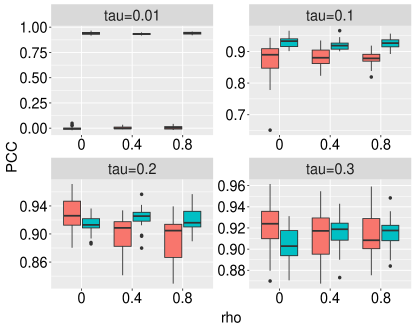
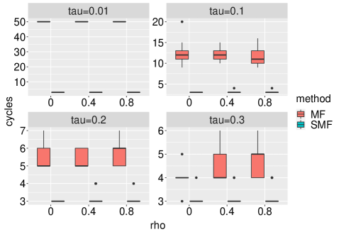
Figure 2: Performance comparison for binary networks between SMF and MF. The left 4 panels show the boxplots of PCC between true and estimated probabilities; while the right 4 panels show the boxplots of the number of cycles required for convergence.

From Figure 2, it is evident that SMF performs better than MF in terms of recovery of latent distances for most of the cases, except $\tau=0.2,0.3$ and $\rho=0$, where the dependence across time is weak. In addition, SMF uniformly requires fewer iterations to converge in all settings. Moreover, when $\tau$ becomes smaller, the iteration number required for MF is higher, while the number remains almost the same for SMF. In particular, when $\tau=0.01$, MF does not converge after 50 iterations ($10$ times the iteration number required by SMF).

Table 1 reports the median of PCC between true and estimated probabilities for SMF with $\sigma_{0}=0.5$ and known $\tau$ vs. adaptive SMF using (3). It is interesting to observe that adaptively learning the initial and transition variances using the prior (3) leads to no loss of accuracy compared to the case when these parameters are known apriori.

Table 1: Performance comparisons for binary networks between adaptive SMF and SMF with known initial and transition variances. The measure compared are the medians of Pearson correlation coefficient (PCC) between true and estimated probabilities of the repeated simulations.

$\tau$	0.01			0.1
$\rho$	0	0.4	0.8	0	0.4	0.8
Adaptive SMF	0.885	0.888	0.892	0.880	0.910	0.914
SMF	0.887	0.881	0.898	0.897	0.912	0.904
$\tau$	0.2			0.3
$\rho$	0	0.4	0.8	0	0.4	0.8
Adaptive SMF	0.907	0.915	0.918	0.908	0.919	0.923
SMF	0.895	0.918	0.915	0.904	0.919	0.931

Gaussian Networks:

25 replicated datasets are generated from $Y_{ijt}\sim\mathcal{N}(0.1+\boldsymbol{x}_{it}^{\prime}\boldsymbol{x}_{jt},0.1^{2})$ for $i\neq j=1,...,n$ and $t=1,...,T$ where $n=100,\,T=100,\,d=2$. Let $\boldsymbol{x}_{i1}\sim\mathcal{N}((0,0)^{\prime},\tau^{2}\mathbbm{I})$, and transitions $\boldsymbol{x}_{it}=\boldsymbol{x}_{i(t-1)}+\boldsymbol{\epsilon}_{t-1}$, where given any coordinate $j$ for a fixed node $i$, let $[\epsilon_{ij1},...,\epsilon_{ijT}]^{\prime}\sim\mathcal{N}(\boldsymbol{0},\tau^{2}\mathbbm{I})$. The iterations are stopped when the difference between predictive RMSEs in two consecutive cycles is less than $10^{-3}$. In the algorithm, both the initial and transition variances are learned adaptively with prior (3). The prior for the intercept is set to $\mathcal{N}(0,10)$. Table 2 shows the mean of the $25$ replicated simulations. Clearly, SMF performs much better than MF in parameter recovery when the transition is small. The result again reinforces that when the dependence among latent positions is significant, SMF should be adopted.

Table 2: Performance comparison for Gaussian networks between SMF and MF. The measure is the median of root mean square error for estimation of the latent distances of the repeated simulations.

$\tau$	0.001	0.005	0.01	0.05	0.1	0.5
MF	0.0101	0.0105	0.0129	0.0219	0.0205	0.0211
SMF	2.34 $\times 10^{-3}$	5.97 $\times 10^{-3}$	9.53 $\times 10^{-3}$	0.0200	0.0206	0.0210

4.2 Enron email data set

Using the Enron email data set (klimt2004enron), we compare our model with the latent space model with the same likelihood but with an inverse Gamma prior on the transition variance. Enron data consists of emails collected from 2359 employees of the Enron company. From all the emails, we examine a subset consisting of $n=184$ employees communicating among $T=44$ months from Nov. 1998 to June 2002 recorded in the R package networkDynamic (butts2020networkDynamic). The networks depict the email communication status of employees over that period. The edges in the network are ones if one of the corresponding two employees sent at least one email to the other during that month. According to the data set, all networks are sparse and many edges remain unchanged over time. The aim of this study is to determine whether shrinkage on transitions induced by Gamma prior on transition variance can be beneficial for sparse dynamic networks. With the dynamic networks, we consider all the edges to be missed with probability $p=0.01,0.02,...,0.1$ independently, train the two latent space models without the missed data, and then make predictions based on the missed data. We use two criteria for comparison: the testing AUC score and the ratio of true positive detection over all missed edges, which is defined as the ratio of predictive probability greater than 0.5 when the true edge value is $1$ over all missed edges. Since all networks are extreme sparse and negative predictions are trivial, the second criterion above is meaningful. The same SMF variational inference method is used in both latent space models. In both of the latent space models, we assign a latent dimension of $5$, the same initializations and stopping criteria. The variational mean of the latent positions is used to estimate the latent positions.

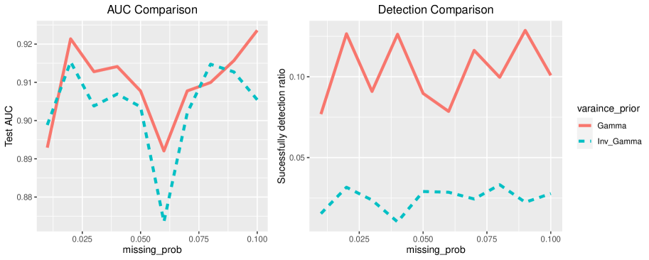
Figure 3: Comparisons of latent space models between Gamma or Inverse Gamma priors on the Enron email testing data.

Figure 3 illustrates performance comparison between the two approaches. The Gamma prior leads to a better fit based on the AUC comparison (left subfigure) and improves on the detection of missed links (right subfigure). A Gamma prior shrinks the transitions more compared to an inverse-Gamma prior so that if two employees communicate at time $t$, the predictive probability for them to communicate at time $t+1$ is high.

4.3 McFarland classroom dataset

McFarland’s streaming classroom dataset provides interactions of conversation turns from streaming observations of a class observed by Daniel McFarland in 1996 (mcfarland2001student). The dataset is available in the R package networkDynamic (butts2020networkDynamic). The class comprised of $2$ instructors and $18$ students. Of the $2$ instructors, one is the main instructor who lectured most of the time while the other is an assistant. During the class, the instructors began by providing instructions to all students. Then the students were divided into groups and assigned collaborative group works. The two instructors oversaw the activities across the groups to assist the students. Here, we aim to compare MF and SMF via prediction accuracy and visualize the dynamic evolution of the latent positions.

We divide the entire class time into $8$ equispaced time points. The edges of each of the $8$ networks represent whether the two nodes interacted related to the study task during the entire time period. We chose $d=2$ for visualization purposes. A $\mathcal{N}(0,10)$ prior is placed on the intercept and the prior (3) is adopted for both SMF and MF.

First, we compare SMF and MF in terms of prediction accuracy. The first $7$ networks are used as the training data, while the last network is used as the test data. The estimated latent positions at time point $7$ are used to predict the probabilities of edges between any two nodes at time $8$. Then the test AUC scores are obtained from the above-estimated probabilities vs. the true binary responses at time point $8$. The final test AUC scores are $0.691$ for MF and $0.738$ for SMF, which again testified to the ability for SMF to capture the dependence across time better.

Next, we implemented SMF with the networks at all 8 time points under the same hyperparameter specification to visualize the dynamic evolution of the latent positions. Since the latent positions estimated directly from the algorithm are not identifiable, Procrustes rotation is performed (hoff2002latent) where the latent positions of time $t=2,..,T$ are projected to the locations that are most close to its previous locations ($t=1,...,T-1$) through Procrustes rotation. Observe that the inner product is invariant to this transformation.

Figure 4 shows the dynamic evolution of the variational mean of the latent positions for both students and instructors (an animated version of Figure 4 is provided in the supplementary material). At time point $1$, (i.e., at the beginning of the class) the students indexed by $\{1,...,20\}\backslash\{7,14\}$ are approximately grouped into the following clusters $(6,11,15)$, $(3,8,13)$, $(10,12,4,5)$, $(1,18,9)$, $(2)$ ,$(19)$ and $(20,17,16)$. The locations of the students remained the same until time point $4$. From time point $4$ to $5$, the inner-group distances between $(13,3,8)$, $(1,9,18)$ and $(4,5,10,12)$ became smaller, which reflected the real scenario that the students were assigned into groups. Then the group structure of the students remained similar for the remainder of the class. Overall, the evolution reflected the collaborative behavior between certain groups as they performed specific tasks during the class. For the instructors (indexed by $7,14$), there were hardly any changes from time point $1$ to $3$. However, from time point $4$ to $7$, the locations of the two instructors changed significantly, as they started providing help across the different groups.

As a point of comparison, we also obtained dynamic visualization of the networks via MF (Figure 5) and the popular ndtv package (ndtv: Network Dynamic Temporal Visualization, skye2021ndtv). Although ndtv package is known for its dynamic networks visualizations through animations, static snapshots of the visualizations can also be created using filmstrip function (Figure 6). First, unlike Figure 4, the latent positions estimated via MF in Figure 5 did not have a smooth temporal evolution, as the MF assumed independence across the time points. In addition, compared to our visualization in Figure 4, results from the ndtv package in Figure 6 lacked a clear pattern of the network evolution. For example, the students indexed $\{1,18,9\}$ stayed close to each other at time points $t=5,6,7$ in Figure 4, while in Figure 6, $18$ is far away from $(1,9)$ at time $t=6$, while being connected to $1$ at the neighboring time points $t=5,7$. Similar phenomenon can be seen for student indexed $5$ at time $t=5$, where in Figure 4 it is close to $(4,10,12)$ while in Figure 6 it is not. The ability of our methodology to borrow information across time is specifically due to the Markovian structure (2) imposed on the evolution of the latent positions endowed with the Gamma prior (3) on the transition variance, allowing sufficient probability near the origin. Thus our methodology revealed a more realistic pattern in the evolution in Figure 4 compared to MF and ndtv as most of the detected changes remained concentrated in time $t=4,5$ for the students (when the students formed groups) and $5,6,7$ for the instructors (after the instructors began assisting the students).

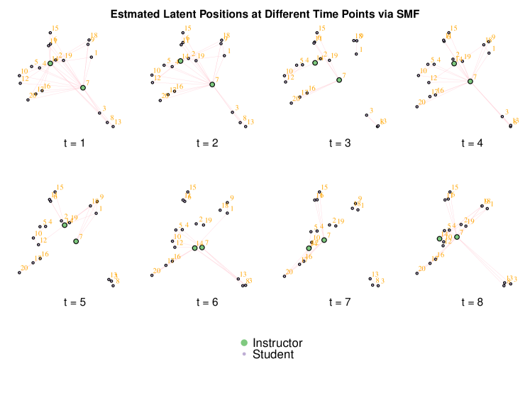
Figure 4: Dynamics of latent positions of all nodes from time point $1$ to $8$ for McFarland classroom dataset via SMF. The locations of the nodes are the estimated latent positions. The edges between two nodes imply the interaction between the two observations within the corresponding time. Each number associated with the point is the index of the node.

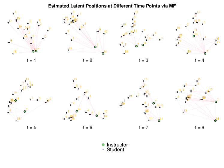
Figure 5: Dynamics of latent positions of all nodes from time point $1$ to $8$ for McFarland classroom dataset via MF. The locations of the nodes are the estimated latent positions. The edges between two nodes imply the interaction between the two observations within the corresponding time. Each number associated with the point is the index of the node.

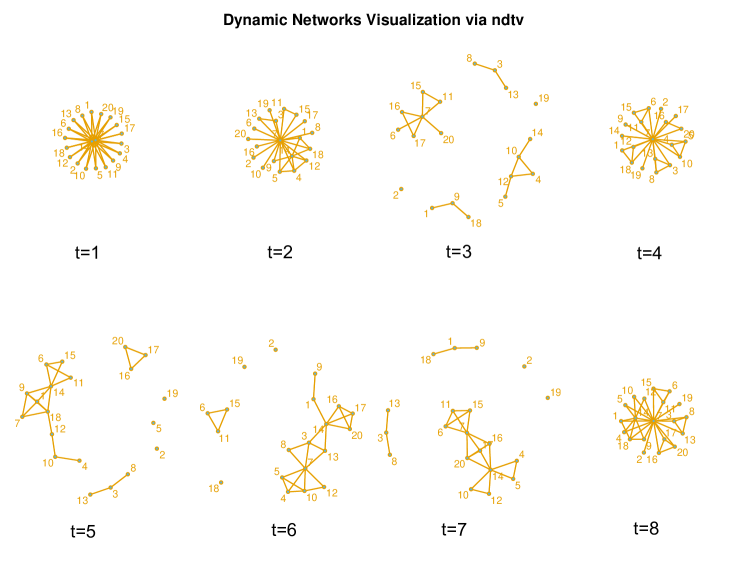
Figure 6: Visualization of the network dynamics from time point $1$ to $8$ for McFarland classroom dataset using R package ndtv. From top left to top right, we have $t=1,...,4$; from bottom left to bottom right, we have $t=5,...,8$. Each number associated with the point is the index of the node.

5 Discussion

There are a number of potential extensions of the proposed methodology and theory in this article. Properties of the Gaussian random walk prior is crucially exploited in our theory to obtain the optimal variational risk. It would be interesting to explore similar theoretical optimality results for Gaussian Process priors (e.g., durante2017bayesian). Moreover, the theoretical analysis of the lower bound can be extended to the case that the true latent positions evolve smoothly over time, like in pensky2019dynamic.

From a methodological point, it is of interest to explore how to perform community detection after estimating the latent positions. As the latent positions are characterized as vectors in the Euclidean space, it is natural to consider some distance-based approaches like K-means for clustering. Adapting to the dimension $d$ of the embedding space is also a challenging problem.

6 Supplementary Material

The supplementary material contains the proofs of the main theorems, the extension to nodewise-adaptive priors (4), algorithm details for MF variational inference and reproducible examples for simulation and real data analysis.

Appendix A Appendix

A.1 Proof of Proposition 2.1

Suppose $q(\beta)$, $q(\tau)$, $q(\sigma_{0})$ and $q(\boldsymbol{x}_{j\cdot})\,,j\neq i$ are given. By the definition of ELBO and equation (9), we have

ELBO $$=\sum_{t=1}^{T-1}\int q_{it,i(t+1)}(\boldsymbol{x}_{it},\boldsymbol{x}_{i(t+1)})\log\psi_{it,i(t+1)}(\boldsymbol{x}_{it},\boldsymbol{x}_{i(t+1)})\mathrm{d}\mathcal{X}$$

$$+\int q_{it}(\boldsymbol{x}_{it})\log\phi_{it}(\boldsymbol{x}_{it})\mathrm{d}\mathcal{X}-\sum_{t=1}^{T}\int q_{it}(\boldsymbol{x}_{it})\log q_{it}(\boldsymbol{x}_{it})\mathrm{d}\mathcal{X}$$

$$-\sum_{t=1}^{T-1}\int q_{it,i(t+1)}(\boldsymbol{x}_{it},\boldsymbol{x}_{i(t+1)})\{\log q_{it,i(t+1)}(\boldsymbol{x}_{it},\boldsymbol{x}_{i(t+1)})$$

$$-\log q_{it}(\boldsymbol{x}_{it})-\log q_{i(t+1)}(\boldsymbol{x}_{i(t+1)})\}\mathrm{d}\mathcal{X}+\mbox{other term.}$$

By introducing Lagrange multiplier $\lambda_{it,i(t+1)}(\boldsymbol{x}_{i(t+1)})$ and $\lambda_{it,i(t-1)}(\boldsymbol{x}_{i(t-1)})$ for the marginalization conditions, for the term related with $q_{it,i(t+1)}(\boldsymbol{x}_{it},\boldsymbol{x}_{i(t+1)})$, we have:

$$\log\psi_{it,i(t+1)}(\boldsymbol{x}_{it},\boldsymbol{x}_{i(t+1)})-\log\frac{q_{it,i(t+1)}(\boldsymbol{x}_{it},\boldsymbol{x}_{i(t+1)})}{q_{it}(\boldsymbol{x}_{it})q_{i(t+1)}(\boldsymbol{x}_{i(t+1)})}-\lambda_{it,i(t+1)}(\boldsymbol{x}_{i(t+1)})-\lambda_{i(t+1),it}(\boldsymbol{x}_{it})+\mbox{constant}=0.$$

For the term related to $q_{it}(\boldsymbol{x}_{it})$, we have:

$$\log\phi_{it}(\boldsymbol{x}_{it})-\log q_{it}(\boldsymbol{x}_{it})+\lambda_{i(t+1),it}(\boldsymbol{x}_{it})+\lambda_{i(t-1),it}(\boldsymbol{x}_{it})+\mbox{constant}=0.$$

Then by combining the above result, we have:

$$q_{it}(\boldsymbol{x}_{it})\propto\phi_{it}(\boldsymbol{x}_{it})\exp(\lambda_{i(t+1),it}(\boldsymbol{x}_{it})+\lambda_{i(t-1),it}(\boldsymbol{x}_{it})),$$ (A.1)

Moreover, we have

$$\begin{aligned} q_{it,i(t+1)}(\boldsymbol{x}_{it},\boldsymbol{x}_{i(t+1)})\propto\phi_{it}(\boldsymbol{x}_{it})\phi_{i(t+1)}(\boldsymbol{x}_{i(t+1)})\psi_{it,i(t+1)}(\boldsymbol{x}_{it},\boldsymbol{x}_{i(t+1)})\\ \cdot\exp(\lambda_{i(t+2),i(t+1)}(\boldsymbol{x}_{i(t+1)})+\lambda_{i(t-1),it}(\boldsymbol{x}_{it})).\end{aligned}$$ (A.2)

Finally, based on the marginalization property of $q_{it,i(t+1)}(\boldsymbol{x}_{it},\boldsymbol{x}_{i(t+1)})$, we have the backward updating:

$$\exp(\lambda_{i(t+1),it}(\boldsymbol{x}_{it}))\propto\int\phi_{i(t+1)}(\boldsymbol{x}_{i(t+1)})\psi_{it,i(t+1)}(\boldsymbol{x}_{it},\boldsymbol{x}_{i(t+1)})\exp(\lambda_{i(t+2),i(t+1)}(\boldsymbol{x}_{i(t+1)}))\mathrm{d}\boldsymbol{x}_{i(t+1)}$$

and forward updating:

$$\exp(\lambda_{it,i(t+1)}(\boldsymbol{x}_{i(t+1)}))\propto\int\phi_{it}(\boldsymbol{x}_{it})\psi_{it,i(t+1)}(\boldsymbol{x}_{it},\boldsymbol{x}_{i(t+1)})\exp(\lambda_{i(t-1),it}(\boldsymbol{x}_{it}))\mathrm{d}\boldsymbol{x}_{it}.$$

Let $m_{it,i(t+1)}(\boldsymbol{x}_{i(t+1)})=\exp(\lambda_{it,i(t+1)}(\boldsymbol{x}_{i(t+1)}))$ and $m_{it,i(t-1)}(\boldsymbol{x}_{i(t-1)})=\exp(\lambda_{it,i(t-1)}(\boldsymbol{x}_{i(t-1)}))$. The equation (13) directly follows equation (A.1) and (A.2) after plugging in the forward and backward messages and therefore the proposition is proved.

A.2 Proof of Theorem 3.1

Within the networks, we adopt the hypotheses constructions for some low-rank matrices, while among the networks, we adopt the test constructions similar to the constructions in total variational literature (padilla2017dfs).

For $\mathcal{U}=\{\boldsymbol{U}_{t}\}_{t=1}^{T}$ with $\boldsymbol{U}_{t}=[\boldsymbol{u}_{1t},...,\boldsymbol{u}_{nt}]^{\prime}$ and $\mathcal{V}=\{\boldsymbol{V}_{t}\}_{t=1}^{T}$ with $\boldsymbol{V}_{t}=[\boldsymbol{v}_{1t},...,\boldsymbol{v}_{nt}]^{\prime}$, let

$$d^{2}(\mathcal{U},\mathcal{V})=\sum_{t=1}^{T}\sum_{i\neq j=1}^{n}(\boldsymbol{u}_{it}^{\prime}\boldsymbol{u}_{jt}-\boldsymbol{v}_{it}^{\prime}\boldsymbol{v}_{jt})^{2},$$

and

$$d_{0}^{2}(\boldsymbol{U}_{t},\boldsymbol{V}_{t})=\sum_{i\neq j=1}^{n}(\boldsymbol{u}_{it}^{\prime}\boldsymbol{u}_{jt}-\boldsymbol{v}_{it}^{\prime}\boldsymbol{v}_{jt})^{2}.$$

Hypothesis constructions for the low-rank part

First we need the following lemma to obtain sparse Varshamov-Gilbert Bound under Hamming distance for the low-rank subset construction:

Lemma A.1 (Lemma 4.10 in massart2007concentration).

Let $\Omega=\{0,1\}^{n}$ and $1\leq s\leq n/4$. Then there exists a subset $\{w^{(1)},...,w^{(M)}\}\subset\Omega$ such that

1. $\|w^{(i)}\|_{0}=s$ for all $1\leq i\leq M$;

2. $\|w^{(i)}-w^{(j)}\|_{0}\geq s/2$ for $0\leq i\neq j\leq M$;

3. $\log M\geq cs\log(n/s)$ with $c\geq 0.233$.

Let $\Omega_{M}=\{\boldsymbol{w}^{(1)},...,\boldsymbol{w}^{(M)}\}\subset\{0,1\}^{(n-d+1)/2}$ constructed based on the above Lemma (the construction holds under $n-d+1\geq 8$). For each $\boldsymbol{w}$, we can construct a $n\times d$ matrix as follows:

$$\boldsymbol{U}^{w}=\begin{bmatrix}\boldsymbol{v}^{w}&\boldsymbol{0}\\ \boldsymbol{0}&\boldsymbol{I}_{d-1}\end{bmatrix}\quad\mbox{with}\quad\boldsymbol{v}^{w}=\begin{bmatrix}1\\ ...\\ 1\\ \epsilon\boldsymbol{w}\end{bmatrix}\in\mathbb{R}^{n-d+1},w\in\Omega_{M}$$

where the first $(n-d+1)/2$ components for $\boldsymbol{v}^{w}$ are all ones.

The effect of this construction is that: for different $\boldsymbol{w}_{1},\boldsymbol{w}_{2}\in\Omega_{M}$, since $s/2\leq\|\boldsymbol{w}_{1}-\boldsymbol{w}_{2}\|_{0}\leq 2s$ and $\|\boldsymbol{U}^{w}\|_{F}\leq\sqrt{n}$, we have

$$d_{0}(\boldsymbol{U}^{w_{1}},\boldsymbol{U}^{w_{2}})\leq\|\boldsymbol{U}^{w_{1}}\boldsymbol{U}^{{}^{\prime}w_{1}}-\boldsymbol{U}^{w_{2}}\boldsymbol{U}^{{}^{\prime}w_{2}}\|_{F}\leq\|\boldsymbol{U}^{w_{1}}(\boldsymbol{U}^{{}^{\prime}w_{1}}-\boldsymbol{U}^{{}^{\prime}w_{2}})\|_{F}+\|(\boldsymbol{U}^{w_{1}}-\boldsymbol{U}^{w_{2}})\boldsymbol{U}^{{}^{\prime}w_{2}}\|_{F}$$

$$\leq 2\sqrt{n}\|\boldsymbol{U}^{w_{1}}-\boldsymbol{U}^{w_{2}}\|_{F}=2\sqrt{n}\|\boldsymbol{v}^{w_{1}}-\boldsymbol{v}^{w_{2}}\|_{2}\leq 2\sqrt{{2ns}}\epsilon.$$

In addition, consider $A:=\{i+(n-d+1)/2:w_{1i}\neq 0\}$, $B:=\{j+(n-d+1)/2:w_{2j}\neq 0\}$, $C:=A\cap B$, where $w_{1i},w_{2j}$ are $i$ and $j$th component of $w_{1}$ and $w_{2}$. We have $|C|\leq s/2$, $|A-C|\geq s/2$ and $|B-C|\geq s/2$. By direct calculation, we have

$$d^{2}_{0}(\boldsymbol{U}^{w_{1}},\boldsymbol{U}^{w_{2}})=\sum_{i\neq j}^{n-d+1}(v^{w_{1}}_{i}v^{w_{1}}_{j}-v^{w_{2}}_{i}v^{w_{2}}_{j})^{2}.$$

By only considering the sum for $i\in\{1,...,(n-d+1)/2\},j\in A-C$ where $v_{i}^{w_{1}}=v_{i}^{w_{2}}=1$ $v^{w_{1}}_{j}=\epsilon$ and $v^{w_{2}}_{j}=0$ and $i\neq j$, we have

$$d^{2}_{0}(\boldsymbol{U}^{w_{1}},\boldsymbol{U}^{w_{2}})\geq\sum_{i=1}^{(n-d+1)/2}\sum_{j\in A-C}(\epsilon{w_{1}}_{j}-\epsilon{w_{2}}_{j})^{2}\geq\frac{s(n-d+1)}{4}\epsilon^{2}.$$

Hypothesis constructions for the total variational denoising part

As in the total variation denoising literature, we partition the set $\{1,...,T\}$ into $m$ groups $S_{1},S_{2},...,S_{m}$ such that $S_{1}=\{1,...,k\}$, $S_{2}=\{k+1,...,2k\}$, …, $S_{m}=\{(m-1)k+1,...,T\}$, where $k$ will be decided later. Then we have $k(m-1)+1\leq T\leq km.$ For simplicity, we assume the partition is even $T=km$, otherwise we can consider $T^{\prime}=km$, which has the same rate with $T$ since $km>T>km-k+1$. As in the literature in nonparametric regression, we need to obtain optimal order of $k$ or $m$.

Let $\boldsymbol{w}_{0}=[0,...,0]^{\prime}\in\mathbb{R}^{(n-d-1)/2}$ and

$$\boldsymbol{U}^{0}=\begin{bmatrix}\boldsymbol{v}^{w_{0}}&\boldsymbol{0}\\ \boldsymbol{0}&\boldsymbol{I}_{d-1}\end{bmatrix}\quad\mbox{with}\quad\boldsymbol{v}^{w_{0}}=\begin{bmatrix}1\\ ...\\ 1\\ \boldsymbol{w}_{0}\end{bmatrix}\in\mathbb{R}^{n-d+1}$$

and $\mathcal{U}^{0}=[\boldsymbol{U}^{0},...,\boldsymbol{U}^{0}]$. We need the Varshamov-Gilbert Bound A.1 again to introduce another binary coding: let $\Omega_{r}=\{\boldsymbol{\phi}^{(1)},...,\boldsymbol{\phi}^{(M_{0})}\}\subset\{0,1\}^{m}$, such that $\|\boldsymbol{\phi}^{(i)}\|_{0}=s_{0}$ with $s_{0}\leq m/4$ for all $1\leq i\leq M_{0}$ and and $\|\boldsymbol{\phi}^{(i)}-\boldsymbol{\phi}^{(j)}\|_{0}\geq s_{0}/2$ for $0\leq i<j\leq M_{0}$ and $\log M_{0}\geq cs_{0}\log(m/s_{0})$ with $c\geq 0.233$. The construction holds under $m\geq 4$.

Then the construction is based on a mixture of product space of $\Omega_{M}$ and group structure for $S_{1},...S_{m}$:

$$\Theta_{\epsilon}=\{\mathcal{X}^{(w,\phi)}_{...}:$$ (A.3)

$$\boldsymbol{X}^{(w,\phi)}_{t}=\boldsymbol{U}^{w^{(i)}},\quad\forall t\in S_{j}\quad\mbox{if}\quad\phi_{j}=1,$$

$$\boldsymbol{X}^{(w,\phi)}_{t}=\boldsymbol{U}^{0},\quad\forall t\in S_{j},\quad\mbox{if}\quad\phi_{j}=0,$$

$$\boldsymbol{w}^{(i)}\in\Omega_{M},\,\forall i=1,...,s_{0},\,\boldsymbol{w}^{(i)}\,\mbox{are chosen with replacement},\quad\boldsymbol{\phi}\in\Omega_{r}\},$$

For example, when $\phi=(0,1,0,1,0,1,...)$, $\boldsymbol{X}^{(w,\phi)}_{1}$,..,$\boldsymbol{X}^{(w,\phi)}_{T}$ is:

$$\underbrace{\boldsymbol{U}^{0},...,\boldsymbol{U}^{0}}_{|S_{1}|},\underbrace{\boldsymbol{U}^{w^{(1)}},...,\boldsymbol{U}^{w^{(1)}}}_{|S_{2}|},\underbrace{\boldsymbol{U}^{0},...,\boldsymbol{U}^{0}}_{|S_{3}|},\underbrace{\boldsymbol{U}^{w^{(2)}},...,\boldsymbol{U}^{w^{(2)}}}_{|S_{4}|},...$$

We have $|\Theta_{\epsilon}|=M_{0}M^{s_{0}}$. In addition, for $\mathcal{U},\mathcal{V}\in\Theta_{\epsilon}$, we have

$$d^{2}(\mathcal{U},\mathcal{V})=\sum_{t=1}^{T}d_{0}^{2}(\boldsymbol{U}_{t},\boldsymbol{V}_{t})\geq ks_{0}\frac{s(n-d+1)}{8}\epsilon^{2}.$$

Besides, the KL divergence between any elements $\mathcal{U}\in\Theta_{\epsilon}$ and $\mathcal{U}^{0}$ can be upper bounded:

$$D_{KL}(P_{\mathcal{U}}\,||\,P_{\mathcal{U}^{0}})\leq C_{0}d^{2}(\mathcal{U},\mathcal{V})\leq 16C_{0}kns_{0}s\epsilon^{2},$$ (A.4)

for some constant $C_{0}>0$ ($C_{0}=1$ for the binary case, $C_{0}=1/(2\sigma^{2})$ for the Gaussian case).

We use the following lemma to finally obtain the minimax lower bounds.

Lemma A.2 (Theorem 2.5 in tsybakov2008introduction).

Suppose $M\geq 2$ and $(\Theta,d)$ contains elements $\theta_{0},...,\theta_{M}$ such that $d(\theta_{i},\theta_{j})\geq 2s>0$ for any $0\leq i\leq j\leq M$ and $\sum_{i=1}^{M}D_{KL}(P_{\theta_{i}},P_{0})/M\leq\alpha\log M$ with $0<\alpha<1/8$. Then we have

$$\inf_{\hat{\theta}}\sup_{\theta\in\Theta}P_{\theta}(d(\hat{\theta},\theta)\geq s)\geq\frac{\sqrt{M}}{1+\sqrt{M}}\left(1-2\alpha-\sqrt{\frac{2\alpha}{\log M}}\right).$$

To adopt the above Lemma, it suffices to show

$$16C_{0}ks_{0}sn\epsilon^{2}\leq\alpha\log(M_{0}M^{s_{0}})=\alpha\log(|\Theta_{\epsilon}|),$$

with $\alpha<1/8$. Let $s=(n-d-1)/8$, $s_{0}=m/4$, according to lemma A.1, it’s enough to set

$$Tn(n-1)\epsilon^{2}\leq\frac{cm\log 4}{4}+\frac{cm(n-d-1)\log 4}{16}=\frac{cm(n-d+7)\log 4}{16},$$ (A.5)

with $c=0.233/C_{0}$.

Minimax rate for point-wise dependence

Based on our construction, $2(m-1)s\epsilon\leq L$ should be satisfied and we consider the following different cases:

Case 1: If there exist constants $c_{0},c_{0}^{\prime}>0$ such that $c_{0}^{\prime}/\sqrt{nT}<L\leq c_{0}(T-1)n^{1/2}$, which results in $16^{3}TL^{2}/\{4sc\log 4\}<T(T-1)^{2}$, and $16^{3}TL^{2}/(4c\log 4s)>36=4*(4-1)^{2}$. Therefore, since $n\geq 2d$, by assigning $\epsilon=L/\{2(m-1)s\}$ it is enough to let $m$ satisfy

$$\frac{TL^{2}}{(m-1)^{2}}\leq\frac{4cms\log 4}{16^{3}},$$

which is

$$m(m-1)^{2}\geq\frac{16^{3}TL^{2}}{4c\log 4s},$$ (A.6)

and $m$ can be chosen within $4\leq m\leq T$. Let $m$ be the least integer such that the above inequality hold, then there exists a constant $c_{2}$, such that $m\leq c_{2}T^{1/3}L^{2/3}n^{-1/3}$, which implies

$$ks_{0}\frac{s(n-d+1)}{8}\epsilon^{2}\gtrsim L^{\frac{2}{3}}n^{\frac{2}{3}}T^{\frac{1}{3}}.$$

Case 2: If there exists a constant $c_{0}>0$ such that $L>c_{0}(T-1)\sqrt{n}$, which results in $16^{3}TL^{2}/\{cs\log 4\}>T(T-1)^{2}$, then we choose $m=T$, $\epsilon=c_{0}/\sqrt{n}$ such that $(m-1)s\epsilon\leq c_{0}(T-1)\sqrt{n}\leq L/2$. Then

$$ks_{0}\frac{s(n-d+1)}{8}\gtrsim Tn.$$

Case 3: If $L<c_{0}^{\prime}/\sqrt{nT}$ for some constant $c_{0}^{\prime}>0$ such that the least integer solution of inequality (A.6) satisfying $m<4$. Then the above hypothesis construction in equation (A.3) doesn’t hold . Instead of considering the construction in equation (A.3), we consider $T$ copies of the same matrix, that implies the choice of $m$ is $1$. Note that the constraint on norm of the difference of the matrix is automatically satisfied when all matrices are the same. By constructing the following subset

$$\Theta_{\epsilon}=\{\mathcal{X}^{(w)}:\boldsymbol{X}^{(w)}_{t}=\boldsymbol{U}^{w},\quad\forall t=1,...,T,\,\boldsymbol{w}\in\Omega_{M}\}.$$ (A.7)

the KL divergence between any elements $\mathcal{U}\in\Theta_{\epsilon}$ and $\mathcal{U}^{0}$ can be upper bounded:

$$D_{KL}(P_{\mathcal{U}}\,||\,P_{\mathcal{U}^{0}})\leq C_{0}d_{0}^{2}(\boldsymbol{U}_{t},\boldsymbol{V}_{t})\leq 16C_{0}Tsn\epsilon^{2},$$ (A.8)

for some constant $C_{0}>0$. Then it suffices to let

$$16Tsn\epsilon^{2}\leq\frac{c(n-d-1)\log 4}{16}\leq\alpha\log(M).$$

Therefore, based on the above equation, we need to choose $\epsilon=\sqrt{1/(nT)}$. Then we have

$$\frac{ks_{0}s(n-d+1)\epsilon^{2}}{8}\gtrsim n.$$

Finally, based on Markov’s inequality, by combining the above three cases, we have

$$\inf_{\hat{\mathcal{X}}}\sup_{\mathcal{X}\in\Theta_{\epsilon}}\operatorname{\mathbf{E}}_{\mathcal{X}}\left[\frac{1}{Tn(n-1)}d^{2}(\hat{\mathcal{X}},\mathcal{X})\right]\gtrsim\min\left\{\frac{L^{\frac{2}{3}}}{n^{\frac{4}{3}}T^{\frac{2}{3}}},\frac{1}{n}\right\}+\frac{1}{nT}.$$

Therefore, the final conclusion holds.

A.3 Proof of Theorem 3.2 (a)

Proof.

Denote the $\epsilon$ ball for KL divergence neighborhood centered at $\mathcal{X}^{*}$ as

$$B_{n}(\mathcal{X}^{*};\epsilon)=\left\{\mathcal{X}\in\Theta:\int p_{\mathcal{X}^{*}}\log(\frac{p_{\mathcal{X}^{*}}}{p_{\mathcal{X}}})d\mu\leq n(n-1)T\epsilon^{2},\int p_{\mathcal{X}^{*}}\log^{2}(\frac{p_{\mathcal{X}^{*}}}{p_{\mathcal{X}}})d\mu\leq n(n-1)T\epsilon^{2}\right\},$$

where $\mu$ is the Lebesgue measure. As discussed in bhattacharya2019bayesian, under the prior concentration condition that

$$\Pi(B_{n}(\mathcal{X}^{*};\epsilon_{n}))\geq e^{-Tn(n-1)\epsilon_{n,T}^{2}},$$

we can obtain the convergence of the $\alpha$-divergence:

$$D_{\alpha}(p_{\mathcal{X}},p_{\mathcal{X}^{*}})=\frac{1}{\alpha-1}\log\int(p_{\mathcal{X}^{*}})^{\alpha}(p_{\mathcal{X}})^{1-\alpha}d\mu.$$

Based on calculation, for Gaussian likelihood, we have $\max\{D_{KL}(p_{\mathcal{X}},p_{\mathcal{X}^{*}}),V_{2}(p_{\mathcal{X}},p_{\mathcal{X}^{*}})\}\lesssim\sum_{i\neq j,t}(\boldsymbol{x}_{it}^{\prime}\boldsymbol{x}_{jt}-\boldsymbol{x}^{*^{\prime}}_{it}\boldsymbol{x}^{*}_{jt})^{2}$ where $V_{2}(p_{\mathcal{X}},p_{\mathcal{X}^{*}})$ is the second moment of KL ball. For the Bernoulli likelihood, by Lemma A.4, we have

$$D_{KL}(p_{\mathcal{X}},p_{\mathcal{X}^{*}})=\int p_{\mathcal{X}^{*}}\log(\frac{p_{\mathcal{X}^{*}}}{p_{\mathcal{X}}})d\mu\leq\sum_{t=1}^{T}\sum_{i\neq j=1}^{n}(\boldsymbol{x}^{\prime}_{it}\boldsymbol{x}_{jt}-\boldsymbol{x}^{*^{\prime}}_{it}\boldsymbol{x}^{*}_{jt})^{2}.$$

Moreover, we have

$$V_{2}(p_{\mathcal{X}},p_{\mathcal{X}^{*}}):=\int p_{\mathcal{X}^{*}}\log^{2}(\frac{p_{\mathcal{X}^{*}}}{p_{\mathcal{X}}})d\mu\leq\sum_{i\neq j=1}^{n}\sum_{t=1}^{T}2p_{x^{*}_{it},x^{*}_{jt}}(\log\frac{p_{x^{*}_{it},x^{*}_{jt}}}{p_{x_{it},x_{jt}}})^{2}+2(1-p_{x^{*}_{it},x^{*}_{jt}})(\log\frac{1-p_{x^{*}_{it},x^{*}_{jt}}}{1-p_{x_{it},x_{jt}}})^{2}.$$ (A.9)

Under the conditions that $p_{x^{*}_{it},x^{*}_{jt}}:=1/\{1+\exp(-\boldsymbol{x}^{*^{\prime}}_{it}\boldsymbol{x}^{*}_{jt})\}$ is bounded away from $0$ and $1$. The right hand side of equation (A.9) is bounded above by $\sum_{i\neq j,t}(\boldsymbol{x}_{it}^{\prime}\boldsymbol{x}_{jt}-\boldsymbol{x}^{*^{\prime}}_{it}\boldsymbol{x}^{*}_{jt})^{2}$ multiplied by some positive constant. Therefore, we also have $\max\{D_{KL}(p_{\mathcal{X}},p_{\mathcal{X}^{*}}),V_{2}(p_{\mathcal{X}},p_{\mathcal{X}^{*}})\}\lesssim\sum_{i\neq j,t}(\boldsymbol{x}_{it}^{\prime}\boldsymbol{x}_{jt}-\boldsymbol{x}^{*^{\prime}}_{it}\boldsymbol{x}^{*}_{jt})^{2}$ for the binary case. Hence we only need to lower bound the prior probability of the set $\{\sum_{i\neq j,t}(\boldsymbol{x}_{it}^{\prime}\boldsymbol{x}_{jt}-\boldsymbol{x}^{*^{\prime}}_{it}\boldsymbol{x}^{*}_{jt})^{2}\leq n(n-1)T\epsilon^{2}\}\supset\{\max_{t}\max_{i\neq j}(\boldsymbol{x}_{it}^{\prime}\boldsymbol{x}_{jt}-\boldsymbol{x}^{*^{\prime}}_{it}\boldsymbol{x}^{*}_{jt})^{2}\leq\epsilon^{2}\}$. Given $i\neq j,t$ we have

$$|\boldsymbol{x}_{it}^{\prime}\boldsymbol{x}_{jt}-\boldsymbol{x}^{*^{\prime}}_{it}\boldsymbol{x}^{*}_{jt}| \leq|(\boldsymbol{x}^{\prime}_{it}-\boldsymbol{x}^{*^{\prime}}_{it})\boldsymbol{x}^{*}_{jt}|+|\boldsymbol{x}^{\prime}_{it}(\boldsymbol{x}_{jt}-\boldsymbol{x}^{*}_{jt})|$$

$$\leq\max_{i}\|\boldsymbol{x}_{it}-\boldsymbol{x}^{*}_{it}\|_{2}(\|\boldsymbol{x}_{it}-\boldsymbol{x}^{*}_{it}\|_{2}+2\|\boldsymbol{x}^{*}_{it}\|_{2})\leq\max_{i}\|\boldsymbol{x}_{it}-\boldsymbol{x}^{*}_{it}\|_{2}(\|\boldsymbol{x}_{it}-\boldsymbol{x}^{*}_{it}\|_{2}+2C).$$

Then when $\max_{i}\|\boldsymbol{x}_{it}-\boldsymbol{x}^{*}_{it}\|_{2}\leq\epsilon/\{(2+c_{0})C\}\leq C$ for some constants $c_{0}>1$, we have

$$\max_{i}\|\boldsymbol{x}_{it}-\boldsymbol{x}^{*}_{it}\|_{2}(2C+\|\boldsymbol{x}_{it}-\boldsymbol{x}^{*}_{it}\|_{2})\leq\frac{\epsilon}{(2+c_{0})C}3C\leq\epsilon.$$

Denote $E_{0}=\max_{i}\|\boldsymbol{x}_{it}-\boldsymbol{x}^{*}_{it}\|_{2}\leq\epsilon/\{(2+c_{0})C\}$, $E_{1}=\{\max_{i,j,t}|(X_{ijt}-X_{ij1})-(X^{*}_{ijt}-X^{*}_{ij1})|\leq\epsilon_{0}\}$, $E_{2}=\{\max_{i,j}|X_{ij1}-X^{*}_{ij1}|\leq\epsilon_{0}\}$ with $\epsilon_{0}=\epsilon/((2+c_{0})C\sqrt{d})$. Then we have

$$\Pi(E_{0})\geq\Pi\left(E_{1}\right)\Pi\left(E_{2}\right)=\prod_{i,j}\Pi\left(\sup_{t\geq 2}|\tilde{X}_{ijt}-\tilde{X}^{*}_{ijt}|\leq{\epsilon_{0}}\right)\prod_{i,j}\Pi\left(|X_{ij1}-X^{*}_{ij1}|\leq{\epsilon_{0}}\right),$$

where $\tilde{X}_{ijt}=X_{ijt}-X_{ij1}$ for all $i,j,t$.

Given $i,j$, $\xi_{ijt}\sim\mathcal{N}(0,\tau^{2})$ for $t\geq 2$, we can denote $\tilde{X}_{ijt}=\sum_{s=1}^{t}\xi_{ijs}$ and $(\tilde{X}_{ij2},...,\tilde{X}_{ijt})^{\prime}\sim\mathcal{N}(\boldsymbol{0},\boldsymbol{\Sigma}_{0})$. Denote $\tilde{\boldsymbol{x}}_{ij}^{*^{\prime}}=(\tilde{X}^{*}_{ij2},...,\tilde{X}^{*}_{ijt})^{\prime}$. Based on multivariate Gaussian concentration through Anderson’s inequality, we have

$$\Pi(E_{1}) \geq\prod_{i,j}P\left(\sup_{t\geq 2}|\tilde{X}_{ijt}-\tilde{X}^{*}_{ijt}|\leq{\epsilon_{0}}\right)$$ (A.10)

$$\geq\prod_{i,j}\exp(-\frac{\tilde{\boldsymbol{x}}_{ij}^{*^{\prime}}\boldsymbol{\Sigma}_{0}^{-1}\tilde{\boldsymbol{x}}_{ij}^{*}}{2})\Pi\left(\sup_{t}|\tilde{X}_{ijt}|\leq{\epsilon_{0}}\right).$$

By the definition of $\boldsymbol{\Sigma}_{0}$, we have

$$-\frac{\tilde{\boldsymbol{x}}_{ij}^{*^{\prime}}\boldsymbol{\Sigma}_{0}^{-1}\tilde{\boldsymbol{x}_{ij}}^{*}}{2}=-\sum_{t=2}^{T}\frac{(\tilde{X}^{*}_{ijt}-\tilde{X}^{*}_{ij(t-1)})^{2}}{2\tau^{2}}=-\sum_{t=2}^{T}\frac{(X^{*}_{ijt}-X^{*}_{ij(t-1)})^{2}}{2\tau^{2}},$$

where $\tilde{X}^{*}_{ij1}=0$. For the second factor in equation (A.10) , given $i,j$, we consider a Gaussian process $\{\tilde{X}_{ij}(s),0\leq s\leq 1\}$ induced by $(\tilde{X}_{ij2},...,\tilde{X}_{ijt})$ such that $\tilde{X}_{ij}((s-2)/(T-2))=\tilde{X}_{ijt}$, $\tilde{X}_{ij}(0)=0$ and all other values are obtained through interpolations: $\tilde{X}_{ij}(s)=w_{0}\tilde{X}_{ij{(t-1)}}+(1-w_{0})\tilde{X}_{ij{t}}$ $\forall w_{0}\in(0,1)$ with $s=w_{0}(t-3)/(T-2)+(1-w_{0})(t-2)/(T-2)$. Then clearly we have

$$\Pi\left(\sup_{t=2,...,T}|\tilde{X}_{ijt}|\leq\delta\right)\geq\Pi\left(\sup_{s\in[0,1]}|\tilde{X}_{ij}(s)|\leq\delta\right),$$

for any $\delta>0$. Denote $\sigma^{2}(h)=E(\tilde{X}(s+h)-\tilde{X}(s))^{2}=hT\tau^{2}$. Then $\sigma^{2}(h)$ is linear in $h$ hence concave. In addition, $\sigma(h)/(h^{1/2})=\sqrt{T\tau^{2}}$, which is non-decreasing in $(0,1)$. Based on Lemma A.3, we have

$$\Pi(\sup_{0\leq s\leq 1}|\tilde{X}(s)|\leq\delta)\geq C_{4}\exp(-C_{3}\frac{T\tau^{2}}{\delta^{2}})$$

for $\delta>0$ with constants $C_{3},C_{4}>0$.

Therefore, for some constant $C_{3},C_{4}>0$, we have

$$\Pi(E_{1})\geq C_{4}\exp{\left[-\sum_{t=2}^{T}\frac{\|\boldsymbol{X}^{*}_{t}-\boldsymbol{X}^{*}_{t-1}\|_{F}^{2}}{2\tau^{2}}-C_{3}\frac{nT\tau^{2}}{\epsilon^{2}}\right]}$$ (A.11)

$$\geq C_{4}\exp{\left[-n\sum_{t=2}^{T}\max_{i}\frac{\|\boldsymbol{x}^{*}_{it}-\boldsymbol{x}^{*}_{i(t-1)}\|_{2}^{2}}{2\tau^{2}}-C_{3}\frac{nT\tau^{2}}{\epsilon^{2}}\right]}.$$

For PWD, with condition (19), we have

$$\Pi(E_{1})\geq C_{4}\exp{\left[-\frac{-C_{0}^{2}L^{2}}{2nT\tau^{2}}-C_{3}\frac{Tn\tau^{2}}{\epsilon^{2}}\right]}.$$

Moreover, by taking that

$$\tau^{2}=\epsilon L/(nT)$$

we can obtain

$$\log\Pi(E_{1})\gtrsim-\frac{L}{\epsilon}.$$

For the initial error concentration $\Pi(E_{2})$, by the mean-zero Gaussian of $X_{ij1}$ for all $i,j$, we have the concentration:

$$\Pi(E_{2})=\prod_{i,j}\Pi\left(|X_{ij1}-X^{*}_{ij1}|\leq{\epsilon_{0}}\right) \geq\frac{1}{(\sqrt{2\pi}\sigma_{0})^{nd}}\exp(-\sum_{i,j}\frac{X^{*2}_{ij1}}{2\sigma_{0}^{2}})(2\epsilon)^{nd}$$

$$\gtrsim\exp\left[-\frac{\|\boldsymbol{X}^{*}_{1}\|_{F}^{2}}{2\sigma_{0}^{2}}-nd-nd\log(\frac{1}{\epsilon})\right].$$

Note that $\sigma$ is a constant and $\|\boldsymbol{X}^{*}_{1}\|_{F}^{2}=O(n)$. We have $\log\Pi(E_{2})\gtrsim-n\log({1/\epsilon})$.

Then the rate $\epsilon_{n,T}=L^{1/3}T^{-1/3}n^{-2/3}+\sqrt{\log(nT)/nT}$ can be obtained by letting the smallest possible $\epsilon_{n,T}$ such that $n(n-1)T\epsilon_{n,T}^{2}\gtrsim\max\{L/\epsilon_{n,T},n\log({1/\epsilon_{n,T}})\}$.

Finally, this additive rate helps in the choice of the transition $\tau$. In particular, when $L<\log^{3/2}(nT)\sqrt{n/T}$ such that $L^{1/3}T^{-1/3}n^{-2/3}\lesssim\sqrt{\log(nT)/nT}$, the choice of $\tau$ can be relaxed as long as $-\log\Pi(E_{1})\lesssim n\log(nT)$. Therefore, let $\tau^{2}=\log^{2}(nT)/(nT^{2})$ in this case, we have

$$Tn\tau^{2}/\epsilon_{n,T}^{2}\lesssim n\log(nT),\quad\mbox{and}\quad L^{2}/(nT\tau^{2})=n\log(nT).$$ (A.12)

Therefore, the final choice of $\tau$ that guarantees the optimal convergence rate satisfies $\tau^{2}=\log^{2}(nT)/(nT^{2})+\epsilon_{n,T}L/(nT)$.

By Theorem 3.1 in bhattacharya2019bayesian, the prior concentration $\Pi(B_{n}(\mathcal{X}^{*};\epsilon_{n,T}))\geq\exp(-Tn(n-1)\epsilon_{n,T}^{2})$ implies that the posterior contraction of the averaged $\alpha$-divergence for any $0<\alpha<1$ is at the rate $\epsilon^{2}_{n,T}$. For the Gaussian case, by the direct calculation (gil2013renyi), we can obtain that the $\alpha$-divergence is lower bounded by the squared loss function up to some constant factor when the variance of the likelihood is fixed. For binary case, based on the boundness of the truth and Lemma A.5, which indicates that the $1/2$ divergence is lower bounded by the squared loss function up to some constant factor, we can achieve the results in equation (21).

∎

A.4 Proof of Theorem 3.2 (b)

Proof.

Let $\sigma_{0}^{*2}=1$ and $\tau^{*2}=\epsilon_{n,T}L/(nT)+\log^{2}(nT)/(nT^{2})$. In the proof of Theorem 3.2-(a), we show the prior concentration conditional on $\sigma_{0}=c_{1}\sigma_{0}^{*}$ and $\tau=c_{2}\tau^{*}$ for any constants $c_{1},c_{2}>0$ is sufficient:

$$-\log\{\Pi(B_{n}(\mathcal{X}^{*};\epsilon_{n})\mid c_{1}\sigma_{0}^{*},c_{2}\tau^{*})\}\lesssim Tn(n-1)\epsilon_{n,T}^{2}.$$

Therefore, by limiting on the subset $N(\sigma_{0}^{*},\tau^{*})=\{|\sigma_{0}^{2}-\sigma_{0}^{2*}|\leq\sigma_{0}^{2*}/2,\,|\tau^{2}-\tau^{2*}|\leq\tau^{2*}/2\}$ , we have $-\log\Pi(B_{n}(\mathcal{X}^{*};\epsilon_{n})\mid\sigma_{0},\tau)\lesssim Tn(n-1)\epsilon_{n,T}^{2}$. Then

$$\int_{N(\sigma_{0}^{*},\tau^{*})}\Pi(B_{n}(\mathcal{X}^{*};\epsilon_{n})p(\tau)p(\sigma_{0})d\tau\sigma_{0}\gtrsim P(|\tau^{2}-\tau^{*2}|\leq\tau^{*2}/2)P(|\sigma_{0}^{2}-\sigma_{0}^{*2}|\leq\sigma_{0}^{*2}/2)\exp(-Tn(n-1)c_{0}\epsilon_{n,T}^{2}),$$

for some constant $c_{0}>0$. For $\sigma_{0}$, with the Inverse-gamma$(a_{\sigma_{0}},b_{\sigma_{0}})$ prior where $a_{\sigma_{0}},b_{\sigma_{0}}$ are constants, we have

$$P(|\sigma_{0}^{2}-\sigma_{0}^{*2}|\leq\sigma_{0}^{*2}/2)=P(1/2\leq\sigma_{0}^{2}\leq 3/2),$$

which is a fixed constant. For $\tau$, with the Gamma$(c_{\tau},d_{\tau})$ prior where $c_{\tau},d_{\tau}$ are constants, we have

$$P(|\tau^{2}-\tau^{*2}|\leq\tau^{*2}/2)=\int_{\epsilon_{n,T}L/(2nT)+\log^{2}(nT)/(2nT^{2})}^{3\epsilon_{n,T}L/(2nT)+3\log^{2}(nT)/(2nT^{2})}f_{c_{\tau},d_{\tau}}(\tau^{2})d\tau^{2}$$

$$\geq\min_{|\tau^{2}-\tau^{*2}|\leq\tau^{*2}/2}f_{c_{\tau},d_{\tau}}(\tau^{2})\left\{\epsilon_{n,T}L/(2nT)+\log^{2}(nT)/(2nT^{2})\right\},$$

where $f_{c_{\tau},d_{\tau}}(\tau^{2})$ is the density function of Gamma$(c_{\tau},d_{\tau})$ prior. When $|\tau^{2}-\tau^{*2}|\leq\tau^{*2}/2$, we have

$$-\log\{\min_{|\tau^{2}-\tau^{*2}|\leq\tau^{*2}/2}f_{c_{\tau},d_{\tau}}(\tau^{2})\}\lesssim\tau^{*2}-\log(\tau^{*2})\lesssim\epsilon_{n,T}L/(nT)+\log^{2}(nT)/(4nT^{2})+\log(nT).$$

Note that $\epsilon_{n,T}=o(1)$ due to $L=o(n^{2}T)$, we have

$$\epsilon_{n,T}L/(nT)\lesssim L/(nT)\lesssim n\lesssim n\log(nT)\lesssim n(n-1)T\epsilon_{n,T}^{2}.$$

In addition, $\log^{2}(nT)/(4nT^{2})+\log(nT)\lesssim n(n-1)T\epsilon_{n,T}^{2}$ holds.

Moreover, we also have $-\log(\epsilon_{n,T}L/(nT)+\log^{2}(nT)/(2nT^{2}))\lesssim\log(nT)\lesssim n(n-1)T\epsilon_{n,T}^{2}$. Therefore, we showed that under the prior $\Pi$, it holds that $-\log\Pi(|\tau^{2}-\tau^{*2}|\leq\tau^{*2}/2)\lesssim Tn(n-1)\epsilon_{n,T}^{2}$. Hence we have

$$\Pi(B_{n}(\mathcal{X}^{*};\epsilon_{n}))\geq\exp(-Tn(n-1)M\epsilon_{n,T}^{2})$$

for large enough constant $M>0$. With the choice $\epsilon_{n,T}^{new}=\sqrt{M}\epsilon_{n,T}$, we showed that the prior concentration is sufficient enough, and the rest of the proof is similar with Theorem 3.2 (a) by applying Theorem 3.1 in bhattacharya2019bayesian. ∎

A.5 Proof of Theorem 3.3 (a)

Proof.

The proof is based on Theorem 3.3 in yang2020alpha, where we need to provide upper bounds for

$$-\int\log\frac{P(\mathcal{Y}\mid\mathcal{X})}{P(\mathcal{Y}\mid\mathcal{X}^{*})}q(\mathcal{X})d\mathcal{X}$$

and

$$D_{KL}(q(\mathcal{X})\,||\,p(\mathcal{X})),$$

where $q(\mathcal{X})$ is a variational distribution in the SMF family and $p(\mathcal{X})$ is the prior. Based on the definition of $E_{0}$ in the proof in subsection A.3, we have

$$B_{n}(\mathcal{X}^{*};\epsilon)\supset E_{0}:=\{\max_{i,t}\|\boldsymbol{x}_{it}-\boldsymbol{x}_{it}^{*}\|_{2}\leq\epsilon_{0}\},$$

with $\epsilon_{0}=c_{1}\epsilon_{n,T}$, for constant $c_{1}>0$. The above constraint can be written in a separate form:

$$E_{0}=\cap_{i,t}\{\|\boldsymbol{x}_{it}-\boldsymbol{x}_{it}^{*}\|_{2}\leq\epsilon_{0}\}.$$

Then we can choose $q(\mathcal{X})$ in the following way:

$$q(\mathcal{X})\propto\prod_{i=1}^{n}\prod_{t=2}^{T}p(\boldsymbol{x}_{it}\mid\boldsymbol{x}_{i(t-1)})\mathbbm{1}\{\|\boldsymbol{x}_{it}-\boldsymbol{x}_{it}^{*}\|_{2}\leq\epsilon_{0}\}\prod_{i=1}^{n}p(\boldsymbol{x}_{i1})\mathbbm{1}\{\|\boldsymbol{x}_{i1}-\boldsymbol{x}_{i1}^{*}\|_{2}\leq\epsilon_{0}\},$$

where $p(\boldsymbol{x}_{it}\mid\boldsymbol{x}_{i(t-1})$ and $p(\boldsymbol{x}_{i1})$ are components of priors. Note that the above variational distribution belongs to the SMF distribution family. We prove the above two bounds based on the current construction of $q(\mathcal{X})$. First, by Fubini’s theorem and the definition of the prior, we have

$$\operatorname{\mathbf{E}}_{\mathcal{X}^{*}}\left[-\int_{\mathcal{X}}q(\mathcal{X})\log\frac{P(\mathcal{Y}\mid\mathcal{X})}{P\left(\mathcal{Y}\mid\mathcal{X}^{*}\right)}d\mathcal{X}\right]$$

$$=\int_{\mathcal{X}}-\operatorname{\mathbf{E}}_{\mathcal{X}^{*}}\left[\log\frac{P(\mathcal{Y}\mid\mathcal{X})}{P\left(\mathcal{Y}\mid\mathcal{X}^{*}\right)}\right]q(\mathcal{X})d\mathcal{X}$$

$$\leq\int_{B_{n}\left(\mathcal{X}^{*},\epsilon\right)}D_{KL}\left[P\left(\mathcal{Y}\mid\mathcal{X}^{*}\right)||P\left(\mathcal{Y}\mid\mathcal{X}\right)\right]q(\mathcal{X})d\mathcal{X}\leq n(n-1)T\epsilon^{2}.$$

Similarly, for the variance, by Jensen’s inequality and Fubini’s theorem, we have

$$\mbox{Var}_{\mathcal{X}^{*}}\left[\int_{\mathcal{X}}q(\mathcal{X})\log\frac{P(\mathcal{Y}\mid\mathcal{X})}{P\left(\mathcal{Y}\mid\mathcal{X}^{*}\right)}d\mathcal{X}\right]$$

$$\leq\operatorname{\mathbf{E}}_{\mathcal{X}^{*}}\left[\int_{\mathcal{X}}q(\mathcal{X})\log\frac{P(\mathcal{Y}\mid\mathcal{X})}{P\left(\mathcal{Y}\mid\mathcal{X}^{*}\right)}d\mathcal{X}\right]^{2}$$

$$\leq\int_{B_{n}\left(\mathcal{X}^{*},\epsilon\right)}V_{2}\left[P\left(\mathcal{Y}\mid\mathcal{X}^{*}\right)||P\left(\mathcal{Y}\mid\mathcal{X}\right)\right]q(\mathcal{X})d\mathcal{X}\leq n(n-1)T\epsilon^{2}.$$

Therefore, by Chebyshev’s inequality, for any $D>1$, based on the first and second moments of the above bounds, we have

$$P_{\mathcal{X}^{*}}\left[\int_{\mathcal{X}}q(\mathcal{X})\log\frac{P(\mathcal{Y}\mid\mathcal{X})}{P\left(\mathcal{Y}\mid\mathcal{X}^{*}\right)}d\mathcal{X}\leq-Dn(n-1)T\epsilon^{2}\right]$$

$$\leq P_{\mathcal{X}^{*}}\left[\int_{\mathcal{X}}q(\mathcal{X})\log\frac{P(\mathcal{Y}\mid\mathcal{X})}{P\left(\mathcal{Y}\mid\mathcal{X}^{*}\right)}d\mathcal{X}\right.$$

$$\left.-\operatorname{\mathbf{E}}\left\{\int_{\mathcal{X}}q(\mathcal{X})\log\frac{P(\mathcal{Y}\mid\mathcal{X})}{P\left(\mathcal{Y}\mid\mathcal{X}^{*}\right)}d\mathcal{X}\right\}\leq-(D-1)n(n-1)T\epsilon^{2}\right]$$

$$\leq\mbox{Var}_{\mathcal{X}^{*}}\left[\int_{\mathcal{X}}q(\mathcal{X})\log\frac{P(\mathcal{Y}\mid\mathcal{X})}{P\left(\mathcal{Y}\mid\mathcal{X}^{*}\right)}d\mathcal{X}\right]/\left((D-1)^{2}n^{2}(n-1)^{2}T^{2}\epsilon^{4}\right)$$

$$\leq\frac{4}{(D-1)^{2}n(n-1)T\epsilon^{2}}$$

holds with probability $1-1/\{(D-1)^{2}n(n-1)T\epsilon^{2}\}$. ∎

This proves that when $n(n-1)T\epsilon\rightarrow\infty$, we have

$$-\int\log\frac{P(\mathcal{Y}\mid\mathcal{X})}{P(\mathcal{Y}\mid\mathcal{X}^{*})}q(\mathcal{X})d\mathcal{X}\leq Dn(n-1)T\epsilon^{2}$$

with probability converging to one.

In addition, based on the construction of the variational family, we have

$$D_{KL}(q(\mathcal{X})||p(\mathcal{X}))=-\log(\Pi(E_{0})),$$

since for any probability measure $\mu$ and measurable set $A$ with $\mu(A)>0$, we have $D_{KL}(\mu(\cdot\,\cap A)/\mu(A)\,||\,\mu)=-\log(\mu(A))$. By the proof in subsection A.3, we have $-\log(\Pi(E_{0}))\lesssim-\log(\Pi(E_{1}\cap E_{2}))\lesssim\max\{L/\epsilon,n\log({1/\epsilon})\}$ for PWD($L$) with Lipschitz condition. Therefore, the convergence of the $\alpha$-divergence follows by Theorem 3.3 in yang2020alpha. Finally, the $\alpha$-divergence is lower bounded by the loss according to the final part of the proof of Theorem 3.2-(a).

A.6 Proof of Theorem 3.3 (b)

Proof.

Note that the prior now satisfies $p(\mathcal{X},\tau,\sigma_{0})=p(\mathcal{X}\mid\tau,\sigma_{0})p(\tau)p(\sigma_{0})$ and the variational distribution instead satisfies $q(\mathcal{X},\tau,\sigma_{0})=\prod_{i=1}^{n}q_{i}(\boldsymbol{x}_{i\cdot})q(\tau)q(\sigma_{0})$. Let $\sigma_{0}^{*2}=1$ and $\tau^{*2}=\epsilon_{n,T}L/(nT)+\log^{2}(nT)/(nT^{2})$, we consider the following variational distribution:

$$\begin{aligned} q(\mathcal{X},\tau,\sigma_{0})\propto\prod_{i=1}^{n}\prod_{t=2}^{T}p(\boldsymbol{x}_{it}\mid\boldsymbol{x}_{i(t-1)},\tau^{*})\mathbbm{1}\{\|\boldsymbol{x}_{it}-\boldsymbol{x}_{it}^{*}\|_{2}\leq c\epsilon_{n,T}\}\\ \times\prod_{i=1}^{n}p(\boldsymbol{x}_{i1}\mid\sigma_{0}^{*})\mathbbm{1}\{\|\boldsymbol{x}_{i1}-\boldsymbol{x}_{i1}^{*}\|_{2}\leq c\epsilon_{n,T}\}\\ \times p(\tau)\mathbbm{1}\{\tau^{*2}<\tau^{2}<\tau^{*2}e^{\epsilon_{n,T}^{2}}\}p(\sigma_{0})\mathbbm{1}\{\sigma_{0}^{*2}<\sigma_{0}^{2}<\sigma_{0}^{*2}e^{\epsilon_{n,T}^{2}}\}.\end{aligned}$$ (A.13)

Given the prior, we still check the conditions

$$-\int\log\frac{P(\mathcal{Y}\mid\mathcal{X})}{P(\mathcal{Y}\mid\mathcal{X}^{*})}q(\mathcal{X},\tau,\sigma_{0})d\mathcal{X}d\tau d\sigma_{0}\lesssim Tn(n-1)\epsilon_{n,T}^{2}$$ (A.14)

$$D_{KL}(q(\mathcal{X},\tau,\sigma_{0})\,||\,p(\mathcal{X},\tau,\sigma_{0}))\lesssim Tn(n-1)\epsilon_{n,T}^{2}$$ (A.15)

First, the condition (A.14) directly follows the proof of Theorem 3.3 (a) given the MF structure $q(\mathcal{X},\tau,\sigma_{0})=q(\mathcal{X})q(\tau)q(\sigma_{0})$.

Then by the chain rule of KL divergence, we have

$$\begin{aligned} D_{KL}(q(\mathcal{X},\tau,\sigma_{0})\,||\,p(\mathcal{X},\tau,\sigma_{0}))=D_{KL}(q(\tau)||p(\tau))+D_{KL}(q(\sigma_{0})||p(\sigma_{0}))\\ +\int q(\tau)q(\sigma_{0})\int q(\mathcal{X})\log\frac{q(\mathcal{X})}{p(\mathcal{X}|\tau,\sigma_{0})}d\mathcal{X}d\tau d\sigma_{0}.\end{aligned}$$ (A.16)

With the Gamma$(c_{\tau},d_{\tau})$ prior and $\epsilon_{n,T}<1$, we have

$$\begin{aligned} D_{KL}(q(\tau)||p(\tau))&=-\log(P(\tau^{*2}<\tau^{2}<\tau^{*2}e^{\epsilon_{n,T}^{2}}))\\ &\leq-\log(\min_{\tau^{*2}<\tau^{2}<\tau^{*2}e^{\epsilon_{n,T}^{2}}}f_{c_{\tau},d_{\tau}}(\tau^{2})(e^{\epsilon_{n,T}^{2}}-1))\\ &\stackrel{{\scriptstyle(i)}}{{\leq}}-\log(\epsilon_{n,T}^{2})-\log(\min_{\tau^{*2}<\tau^{2}<\tau^{*2}e^{\epsilon_{n,T}^{2}}}f_{c_{\tau},d_{\tau}}(\tau^{2}))\\ &\stackrel{{\scriptstyle(ii)}}{{\lesssim}}Tn(n-1)\epsilon_{n,T}^{2}-\log(\min_{\tau^{*2}<\tau^{2}<\tau^{*2}e^{\epsilon_{n,T}^{2}}}f_{c_{\tau},d_{\tau}}(\tau^{2})),\end{aligned}$$ (A.17)

where in $(i)$ we use $e^{x}-1\geq x$ for any $x$ and $(ii)$ is because $\epsilon_{n,T}^{2}\geq\log(nT)/(nT)$. In addition, by the similar approach with proof in Theorem 3.2 (b), we have

$$-\log(\min_{\tau^{*2}<\tau^{2}<\tau^{*2}e^{\epsilon_{n,T}^{2}}}f_{c_{\tau},d_{\tau}}(\tau^{2}))\lesssim\tau^{*2}-\log(\tau^{*2})\lesssim n(n-1)T\epsilon_{n,T}^{2}.$$

With $\epsilon_{n,T}<1$, we have $1<\sigma_{0}^{2}<e$ in the constrained region, where the density of Inverse-Gamma$(a_{\sigma_{0}},b_{\sigma_{0}})$ is lower bounded by a constant. Hence,

$$D_{KL}(q(\sigma_{0})||p(\sigma_{0}))=-\log(P(\sigma_{0}^{*2}<\sigma_{0}^{2}<\sigma_{0}^{*2}e^{\epsilon_{n,T}^{2}}))\lesssim-\log(\epsilon_{n,T}^{2})\stackrel{{\scriptstyle(i)}}{{\lesssim}}Tn(n-1)\epsilon_{n,T}^{2},$$ (A.18)

where $(i)$ is due to $\epsilon_{n,T}^{2}\geq\log(nT)/(nT)$. For the third term of the KL divergence, we have

$$\int q(\mathcal{X})\log\frac{q(\mathcal{X})}{p(\mathcal{X}|\tau,\sigma_{0})}d\mathcal{X}=\int_{E_{0}}q(\mathcal{X})\log\frac{p(\mathcal{X}|\tau^{*},\sigma^{*}_{0})}{p(\mathcal{X}|\tau,\sigma_{0})}d\mathcal{X}-\log(\Pi(E_{0}\mid\tau^{*},\sigma_{0}^{*})).$$

Note that we already have $-\log(\Pi(E_{0}\mid\tau^{*},\sigma_{0}^{*}))\lesssim Tn(n-1)\epsilon_{n,T}^{2}$ by the proof of the prior concentration in subsection A.3.

Moreover, we have the density,

$$p(\mathcal{X}\mid\tau,\sigma_{0})=\frac{1}{(\sqrt{2\pi})^{nTd}}\exp\left\{-\frac{n(T-1)d}{2}\log(\tau^{2})-\frac{nd}{2}\log(\sigma_{0}^{2})-\frac{\|\boldsymbol{X}_{1}\|_{F}^{2}}{2\sigma_{0}^{2}}-\frac{\sum_{t=2}^{T}\|\boldsymbol{X}_{t}-\boldsymbol{X}_{t-1}\|_{F}^{2}}{2\tau^{2}}\right\},$$

which implies that

$$\log\frac{p(\mathcal{X}|\tau^{*},\sigma^{*}_{0})}{p(\mathcal{X}|\tau,\sigma_{0})}=\frac{n(T-1)d}{2}\log(\tau^{2})-\frac{n(T-1)d}{2}\log(\tau^{*2})+\frac{nd}{2}\log(\sigma_{0}^{2})-\frac{nd}{2}\log(\sigma_{0}^{*2})$$

$$+\frac{\|\boldsymbol{X}_{1}\|_{F}^{2}}{2\sigma_{0}^{2}}-\frac{\|\boldsymbol{X}_{1}\|_{F}^{2}}{2\sigma_{0}^{*2}}+\frac{\sum_{t=2}^{T}\|\boldsymbol{X}_{t}-\boldsymbol{X}_{t-1}\|_{F}^{2}}{2\tau^{2}}-\frac{\sum_{t=2}^{T}\|\boldsymbol{X}_{t}-\boldsymbol{X}_{t-1}\|_{F}^{2}}{2\tau^{*2}}.$$

With the constrained region $\tau^{*2}<\tau^{2}<\tau^{*2}e^{\epsilon_{n,T}^{2}}$ and $\sigma_{0}^{*2}<\sigma_{0}^{2}<\sigma_{0}^{*2}e^{\epsilon_{n,T}^{2}}$, we have,

$$\log\frac{p(\mathcal{X}|\tau^{*},\sigma^{*}_{0})}{p(\mathcal{X}|\tau,\sigma_{0})}\leq\frac{n(T-1)d}{2}\epsilon_{n,T}^{2}+\frac{nd}{2}\epsilon_{n,T}^{2}\lesssim Tn(n-1)\epsilon_{n,T}^{2},$$

which implies that the third term of the KL divergence (A.16) is also bounded by $Tn(n-1)\epsilon_{n,T}^{2}$. Therefore, we proved that condition (A.15) is satisfied.

Finally, the conclusion holds by applying similar arguments in the final part of the proof of Theorem 3.3 (a).

∎

A.7 Nodewise adaptive priors

In this section, we consider the likelihood (1) with nodewise adaptive priors:

$$\begin{aligned} \boldsymbol{x}_{i1}&\sim\mathcal{N}(\boldsymbol{0},\sigma_{0i}^{2}\mathbb{I}_{d}),\quad&\boldsymbol{x}_{i(t+1)}\mid\boldsymbol{x}_{it}\sim\mathcal{N}(\boldsymbol{x}_{it},\tau_{i}^{2}\mathbb{I}_{d}),\\ \sigma_{0i}^{2}&\sim\mbox{Inverse-Gamma}\left(a_{\sigma_{0}},b_{\sigma_{0}}\right),\quad&\tau_{i}^{2}\sim\mbox{Gamma}\left(c_{\tau},d_{\tau}\right),\end{aligned}$$ (A.19)

for $i=1,...,n;t=1,...,T-1$ to capture the nodewise level differences. The SMF are now in the following form:

$$q(\mathcal{X},\boldsymbol{\tau},\boldsymbol{\sigma}_{0},\beta)=\prod_{i=1}^{n}q_{i}(\boldsymbol{x}_{i\cdot})q(\tau_{i})q(\sigma_{0i})q(\beta).$$ (A.20)

First, there are only minimal changes in the computational framework. First, for the $q_{i}(\boldsymbol{x}_{i\cdot})$ updatings, we have the graph potentials $\boldsymbol{x}_{i\cdot}$ as follows:

$$\begin{aligned} &\phi_{i1}(\boldsymbol{x}_{i1})=\exp\{-\mu_{1/\tau_{i}^{2}}\|\boldsymbol{x}_{i1}\|_{2}^{2}/2-\mu_{1/\sigma_{0i}^{2}}\|\boldsymbol{x}_{i1}\|_{2}^{2}/2\}\prod_{j\neq i}\exp[\operatorname{\mathbf{E}}_{q(\beta)q(\boldsymbol{x}_{j1})}\{\log P_{\alpha}(Y_{ij1}\mid\boldsymbol{x}_{i1},\boldsymbol{x}_{j1},\beta)\}],\\ &\phi_{it}(\boldsymbol{x}_{it})=\exp\{-\mu_{1/\tau_{i}^{2}}\|\boldsymbol{x}_{it}\|_{2}^{2}/2\}\prod_{j\neq i}\exp[\operatorname{\mathbf{E}}_{q(\beta)q(\boldsymbol{x}_{jt})}\{\log P_{\alpha}(Y_{ij1}\mid\boldsymbol{x}_{it},\boldsymbol{x}_{jt},\beta)\}],\,\forall t\in\{2,...,T\}\\ &\psi_{it,i(t+1)}(\boldsymbol{x}_{it},\boldsymbol{x}_{i(t+1)})=\exp(\mu_{1/\tau_{i}^{2}}\boldsymbol{x}_{i(t+1)}^{\prime}\boldsymbol{x}_{it}),\,\forall t\in\{1,...,T-1\},\end{aligned}$$

where $\mu_{1/\tau_{i}^{2}}=\operatorname{\mathbf{E}}_{q(\tau_{i})}(1/\tau_{i}^{2})$ and $\mu_{1/\sigma_{0i}^{2}}=\operatorname{\mathbf{E}}_{q(\sigma_{0i})}(1/\sigma_{0i}^{2})$. Then the updating of $q_{i}(\boldsymbol{x}_{i\cdot})$ follows the same MP framework under the above revised potentials. In addition, for the updating of scales, we have

$$\begin{aligned} q^{(new)}(\tau_{i}^{2})&\propto\exp\left[\operatorname{\mathbf{E}}_{q_{i}(\boldsymbol{x}_{i\cdot})}\left\{-\sum_{t=2}^{T}\frac{\|\boldsymbol{x}_{it}-\boldsymbol{x}_{i(t-1)}\|_{2}^{2}}{2\tau_{i}^{2}}\right\}-\frac{(T-1)d+c_{\tau}-1}{2}\log(\tau_{i}^{2})-d_{\tau}\tau_{i}^{2}\right].\\ q^{(new)}(\sigma_{0i}^{2})&\propto\exp\left[\operatorname{\mathbf{E}}_{q(\boldsymbol{x}_{i1})}\left(-\frac{\|\boldsymbol{x}_{i1}\|_{2}^{2}}{2\sigma_{0i}^{2}}\right)-\left(\frac{d}{2}+a_{\sigma_{0}}+1\right)\log(\sigma_{0i}^{2})-\frac{b_{\sigma_{0}}}{\sigma_{0i}^{2}}\right].\end{aligned}$$ (A.21)

Therefore, we can obtain the that new update of $q(\tau_{i}^{2})$ follows a Generalized inverse Gaussian distribution with parameter $a=2d_{\tau},b=\operatorname{\mathbf{E}}_{q_{i}(\boldsymbol{x}_{i\cdot})}\{\sum_{t=2}^{T}\|\boldsymbol{x}_{it}-\boldsymbol{x}_{i(t-1)}\|_{2}^{2}/2\},p=1/2-(T-1)d/2-c_{\tau}/2$. Then the moment required in updating $\boldsymbol{x}_{it}$ can be obtained: $\operatorname{\mathbf{E}}_{q(\tau_{i})}(1/\tau_{i}^{2})=K_{p+1}(\sqrt{b})/\left\{\sqrt{b}K_{p}(\sqrt{b})\right\}-2p/b$, where $K_{p}(\cdot)$ is the modified Bessel function of the second kind. In addition, the new update of $\sigma_{0i}^{(new)2}\sim$ Inverse-Gamma$((d+a_{\sigma_{0}})/2,\{\operatorname{\mathbf{E}}_{q(\boldsymbol{x}_{i1})}(\|\boldsymbol{x}_{i1}\|_{2}^{2})+2b_{\sigma_{0i}}\}/2)$, which implies $\mu_{1/\sigma_{0i}^{2}}=\operatorname{\mathbf{E}}_{q(\sigma_{0i})}(1/\sigma_{0i}^{2})=(d+a_{\sigma_{0}})/\{\operatorname{\mathbf{E}}_{q(\boldsymbol{x}_{i1})}(\|\boldsymbol{x}_{i1}\|_{2}^{2})+2b_{\sigma_{0}}\}$.

The theoretical results can also be obtained similarly:

Theorem A.1 (Fractional posterior convergence rate for nodewise adaptive priors).

Suppose the true data generating process satisfies equation (16), $\mathcal{X}^{*}\in\mbox{PWD}(L)$ with $0\leq L=o(Tn^{2})$ and conditions (18) and (19) hold. Suppose $d$ is a known fixed constant. Let $\epsilon_{n,T}=L^{1/3}/(T^{1/3}n^{2/3})+\sqrt{\log(nT)/(nT)}$. Then if we apply the priors defined in equation (2) and adopt priors (A.19) for $\sigma_{0i}$ and $\tau_{i}$, we have for $n,T\rightarrow\infty$,

$$\operatorname{\mathbf{E}}\left[\Pi_{\alpha}\left\{\frac{1}{Tn(n-1)}\sum_{t=1}^{T}\sum_{i\neq j=1}^{n}\left(\hat{\boldsymbol{x}}^{\prime}_{it}\hat{\boldsymbol{x}}_{jt}-\boldsymbol{x}_{it}^{*^{\prime}}\boldsymbol{x}_{jt}^{*}\right)^{2}\geq M\epsilon^{2}_{n,T}\mid\mathcal{Y}\right\}\right]\rightarrow 0,$$ (A.22)

with $P_{\mathcal{X}^{*}}$ probability converging to one, where $M>0$ is a large enough constant.

Proof.

The proof is similar to proof of Theorem 3.2 (b) in section A.4. It suffices to show that the prior concentration for the set $N(\sigma_{0}^{*},\tau^{*})=\{|\sigma_{0i}^{2}-\sigma_{0}^{*2}|\leq\sigma_{0}^{*2}/2,\,|\tau_{i}^{2}-\tau^{*2}|\leq\tau^{*2}/2,\,i=1,..,n\}$ is sufficiently large. Due to the independence of the prior, we have

$$-\log P(|\sigma_{0i}^{2}-\sigma_{0}^{*2}|\leq\sigma_{0}^{*2}/2,i=1,...,n)=-\log\{P(|\sigma_{01}^{2}-\sigma_{0}^{*2}|)^{n}\}\lesssim n\lesssim n(n-1)T\epsilon_{n,T}^{2}.$$

Similarly,

$$-\log P(|\tau_{i}^{2}-\tau^{*2}|\leq\tau^{*2}/2,i=1,...,n)=-n\log\{P(|\tau_{1}^{2}-\tau^{*2}|\leq\tau^{*2}/2)\}$$

$$\lesssim-n\log(\epsilon_{n,T}L/(nT)+\log^{2}(nT)/(2nT^{2}))+n\tau^{*2}-n\log(\tau^{*2}).$$

Since $\log^{2}(nT)/(nT^{2})\leq\tau^{*2}\leq L/(nT)+\log^{2}(nT)/(nT^{2})$, we have $-n\log(\log^{2}(nT)/(2nT^{2}))\lesssim n\log(nT)$; $n\tau^{*2}\leq L/T+\log^{2}(nT)/T^{2}\lesssim n\log(nT)$ and $-n\log(\tau^{*2})\lesssim n\log(nT)$. Therefore, we show that $-\log\Pi(N(\sigma_{0}^{*},\tau^{*}))\lesssim n(n-1)T\epsilon_{n,T}^{2}$, then the rest of the proof follows the same with section A.4.

∎

Theorem A.2 (Variational risk bound for nodewise adaptive SMF).

Suppose the true data generating process satisfies equation (16), $\mathcal{X}^{*}\in\mbox{PWD}(L)$ with $0\leq L=o(Tn^{2})$ and conditions (18) and (19) hold. Suppose $d$ is a known fixed constant. Let $\epsilon_{n,T}=L^{1/3}/(T^{1/3}n^{2/3})+\sqrt{\log(nT)/nT}$. Then if we apply the priors defined in equation (2) and adopt priors (A.19) for $\sigma_{oi}$ and $\tau_{i}$ for $i=1,...,n$ and obtaining the optimal variational distribution $\hat{q}(\mathcal{X})$ under nodewise adaptive SMF family (A.20), we have with $P_{\mathcal{X}^{*}}$ probability tending to one as $n,T\rightarrow\infty$,

$$\operatorname{\mathbf{E}}_{\hat{q}(\mathcal{X})}\left[\frac{1}{Tn(n-1)}\sum_{t=1}^{T}\sum_{i\neq j=1}^{n}\left(\hat{\boldsymbol{x}}^{\prime}_{it}\hat{\boldsymbol{x}}_{jt}-\boldsymbol{x}_{it}^{*^{\prime}}\boldsymbol{x}_{jt}^{*}\right)^{2}\right]\lesssim\epsilon^{2}_{n,T}.$$ (A.23)

Proof.

We consider the following variational distribution:

$$\begin{aligned} q(\mathcal{X},\tau,\sigma_{0})\propto\prod_{i=1}^{n}\prod_{t=2}^{T}p(\boldsymbol{x}_{it}\mid\boldsymbol{x}_{i(t-1)},\tau^{*})\mathbbm{1}\{\|\boldsymbol{x}_{it}-\boldsymbol{x}_{it}^{*}\|_{2}\leq c\epsilon_{n,T}\}\\ \times\prod_{i=1}^{n}p(\boldsymbol{x}_{i1}\mid\sigma_{0}^{*})\mathbbm{1}\{\|\boldsymbol{x}_{i1}-\boldsymbol{x}_{i1}^{*}\|_{2}\leq c\epsilon_{n,T}\}\\ \times\prod_{i=1}^{n}p(\tau_{i})\mathbbm{1}\{\tau^{*2}<\tau_{i}^{2}<\tau^{*2}e^{\epsilon_{n,T}^{2}}\}\prod_{i=1}^{n}p(\sigma_{0i})\mathbbm{1}\{\sigma_{0}^{*2}<\sigma_{0i}^{2}<\sigma_{0}^{*2}e^{\epsilon_{n,T}^{2}}\}.\end{aligned}$$ (A.24)

∎

After the change of the priors and variational family, first by equation (A.18) and $-n\log(\epsilon_{n,T}^{2})\lesssim n\log(nT)$, we have

$$D_{KL}(q(\boldsymbol{\sigma}_{0})||p(\boldsymbol{\sigma}_{0}))=-n\log(P(\sigma_{0}^{*2}<\sigma_{01}^{2}<\sigma_{0}^{*2}e^{\epsilon_{n,T}^{2}}))\lesssim-n\log(\epsilon_{n,T}^{2}){\lesssim}Tn(n-1)\epsilon_{n,T}^{2}.$$

Similarly, by equation (A.17), we also have

$$\begin{aligned} D_{KL}(q(\boldsymbol{\tau})||p(\boldsymbol{\tau}))&=-n\log(P(\tau^{*2}<\tau_{1}^{2}<\tau^{*2}e^{\epsilon_{n,T}^{2}}))\\ &\lesssim-n\log(\epsilon_{n,T}^{2})-n\log(\min_{\tau^{*2}<\tau^{2}<\tau^{*2}e^{\epsilon_{n,T}^{2}}}f_{c_{\tau},d_{\tau}}(\tau^{2}))\\ &\lesssim Tn(n-1)\epsilon_{n,T}^{2}.\end{aligned}$$

Moreover, we have the density,

$$p(\mathcal{X}\mid\boldsymbol{\tau},\boldsymbol{\sigma}_{0})=\frac{1}{(\sqrt{2\pi})^{nTd}}\exp\left\{-\sum_{i=1}^{n}\frac{(T-1)d}{2}\log(\tau_{i}^{2})-\sum_{i=1}^{n}\frac{d}{2}\log(\sigma_{0i}^{2})\right.$$

$$\left.-\sum_{i=1}^{n}\frac{\|\boldsymbol{x}_{i1}\|_{2}^{2}}{2\sigma_{0i}^{2}}-\frac{\sum_{i=1}^{n}\sum_{t=2}^{T}\|\boldsymbol{x}_{it}-\boldsymbol{x}_{i(t-1)}\|_{2}^{2}}{2\tau_{i}^{2}}\right\},$$

which implies that

$$\log\frac{p(\mathcal{X}|\boldsymbol{\tau}^{*},\boldsymbol{\sigma}^{*}_{0})}{p(\mathcal{X}|\boldsymbol{\tau},\boldsymbol{\sigma}_{0})}=\sum_{i=1}^{n}\frac{(T-1)d}{2}\log(\tau_{i}^{2})-\frac{n(T-1)d}{2}\log(\tau^{*2})+\sum_{i=1}^{n}\frac{d}{2}\log(\sigma_{0i}^{2})-\frac{nd}{2}\log(\sigma_{0}^{*2})$$

$$+\sum_{i=1}^{n}\frac{\|\boldsymbol{x}_{i1}\|_{2}^{2}}{2\sigma_{0i}^{2}}-\frac{\|\boldsymbol{X}_{1}\|_{F}^{2}}{2\sigma_{0}^{*2}}+\frac{\sum_{i=1}^{n}\sum_{t=2}^{T}\|\boldsymbol{x}_{it}-\boldsymbol{x}_{i(t-1)}\|_{2}^{2}}{2\tau_{i}^{2}}-\frac{\sum_{t=2}^{T}\|\boldsymbol{X}_{t}-\boldsymbol{X}_{t-1}\|_{F}^{2}}{2\tau^{*2}},$$

where $\boldsymbol{\tau}^{*}=(\tau^{*},\tau^{*},...,\tau^{*})^{\prime}$ and $\boldsymbol{\sigma}_{0}^{*}=(\sigma_{0}^{*},\sigma_{0}^{*},...,\sigma_{0}^{*})^{\prime}$. With the constrained region $\tau^{*2}<\tau^{2}<\tau^{*2}e^{\epsilon_{n,T}^{2}}$ and $\sigma_{0}^{*2}<\sigma_{0}^{2}<\sigma_{0}^{*2}e^{\epsilon_{n,T}^{2}}$, we have,

$$\log\frac{p(\mathcal{X}|\boldsymbol{\tau}^{*},\boldsymbol{\sigma}^{*}_{0})}{p(\mathcal{X}|\boldsymbol{\tau},\boldsymbol{\sigma}_{0})}\leq\frac{n(T-1)d}{2}\epsilon_{n,T}^{2}+\frac{nd}{2}\epsilon_{n,T}^{2}\lesssim Tn(n-1)\epsilon_{n,T}^{2}.$$

Then the rest of the proofs follow the same with proof of Theorem (3.3) in section A.6.

A.8 Auxiliary lemmas

Lemma A.3 (Small ball probability of a Gaussian Process with stationary increments, Theorem 1.1 in shao1993note).

Let $\{X(t),0\leq t\leq 1\}$ be a real-valued Gaussian process with mean zero, $X(0)=0$ and stationary increments. Denote $\sigma^{2}(h)=E(X(t+h)-X(t))^{2}$ for $0\leq t\leq t+h\leq 1$. If $\sigma^{2}(h)$ is concave and $\sigma(h)/h^{\alpha}$ is non-decreasing in $(0,1)$ for some $\alpha>0$, then we have

$$P(\sup_{0\leq t\leq 1}|X(t)|\leq C_{\alpha}\sigma(x))\geq\exp(-2/x),$$

where $C_{\alpha}=1+3e\sqrt{\pi/\alpha}$.

Lemma A.4 (Upper bound for binary KL divergence).

Let $p_{a}=1/(1+\exp(-a))$ and $p_{b}=1/(1+\exp(-b))$. Define $P_{a}$ and $P_{b}$ as the Bernoulli measures with probability $p_{a}$ and $p_{b}$. Then we have

$$D_{KL}(P_{a}\,||\,P_{b})+D_{KL}(P_{b}\,||\,P_{a})\leq(a-b)^{2}.$$

Proof.

$$D_{KL}(P_{a}\,||\,P_{b})+D_{KL}(P_{b}\,||\,P_{a}) =(p_{a}-p_{b})\log\frac{p_{a}}{p_{b}}+(p_{b}-p_{a})\log\frac{1-p_{a}}{1-p_{b}}$$

$$=(p_{a}-p_{b})\log\left(\frac{p_{a}}{1-p_{a}}\frac{1-p_{b}}{p_{b}}\right) =\left\{\frac{1}{1+\exp(-a)}-\frac{1}{1+\exp(-b)}\right\}\log(e^{a}e^{-b})$$

$$=(a-b)\left\{\frac{1}{1+\exp(-a)}-\frac{1}{1+\exp(-b)}\right\}.$$

Without loss of generality, we can assume $a>b$, then by $\exp(x)\geq 1+x$, we have

$$\frac{1}{1+\exp(-a)}-\frac{1}{1+\exp(-b)}=\frac{e^{-b}-e^{-a}}{(1+\exp(-a))(1+\exp(-b))}$$

$$\leq\frac{1-e^{b-a}}{(1+e^{-a})(1+e^{b})}\leq 1-e^{b-a}\leq a-b.$$

∎

Lemma A.5 (Lower bound of the $1/2$ divergence).

Let $p_{a}=1/(1+\exp(-a))$ and $p_{b}=1/(1+\exp(-b))$. Define $P_{a}$ and $P_{b}$ as the Bernoulli measures with probability $p_{a}$ and $p_{b}$. Suppose that there exist constants $c,C>0$ such that $c<a,b<C$, then we have

$$D_{\frac{1}{2}}(P_{a},P_{b})\gtrsim(b-a)^{2}.$$

Proof.

First we have

$$D_{\frac{1}{2}}(p_{a},p_{b})=-2\log(1-h^{2}(p_{a},p_{b}))\geq 2h^{2}(p_{a},p_{b})$$

$$=\left[(\sqrt{p_{a}}-\sqrt{p_{b}})^{2}+(\sqrt{1-p_{a}}-\sqrt{1-p_{b}})^{2}\right].$$

In addition, since $a,b$ are bounded, $p_{a},p_{b}$ are bounded away form $0$ and $1$, and $(\sqrt{p_{a}}+\sqrt{p_{b}}),(\sqrt{1-p_{a}}+\sqrt{1-p_{b}})$ are bounded from $0$ as well. Hence,

$$D_{\frac{1}{2}}(p_{a},p_{b})\gtrsim\left[(\sqrt{p_{a}}-\sqrt{p_{b}})^{2}(\sqrt{p_{a}}+\sqrt{p_{b}})^{2}+(\sqrt{1-p_{a}}-\sqrt{1-p_{b}})^{2}(\sqrt{1-p_{a}}+\sqrt{1-p_{b}})^{2}\right]$$

$$\gtrsim(p_{a}-p_{b})^{2}\stackrel{{\scriptstyle(i)}}{{=}}\left\{\frac{\exp(x)}{(1+\exp(x))^{2}}\right\}^{2}(a-b)^{2}\geq\frac{1}{4}(a-b)^{2}.$$

where $(i)$ is because the mean value theorem and $a<x<b$ is bounded.

∎

Lemma A.6 (Probability bound for maximal of sub-Gaussian random variables).

Let $X_{1},...,X_{n}$ be independent sub-Gaussian random variables with mean zero and sub-Gaussian norm upper bounded by $\sigma$. Then we have for every $t>0$,

$$P\left\{\max_{i=1,...,n}|X_{i}|\geq\sqrt{2\sigma^{2}(\log n+t)}\right\}\leq 2e^{-t}.$$

Proof.

By union bound and the sub-Gaussianity, we have

$$P\left\{\max_{i=1,...,n}|X_{i}|\geq u\right\}\leq\sum_{i=1}^{n}P\{|X_{i}|\geq u\}\leq 2ne^{-\frac{u^{2}}{2\sigma^{2}}},$$

by choosing $u=\sqrt{2\sigma^{2}(\log n+t)}$, the conclusion is proved. ∎

A.9 MF Updatings for $\beta$

Suppose the prior for $\beta$ is $\mathcal{N}(\mu_{\beta},\sigma_{\beta}^{2})$. For Gaussian likelihood, the updating for $\beta$ can be obtained

$$\hat{q}(\beta) \propto\exp[\operatorname{\mathbf{E}}_{-\beta}\{\log p_{\alpha}(\mathcal{X},\beta,\mathcal{Y})\}]\propto\exp[\operatorname{\mathbf{E}}_{-\beta}\{\log P_{\alpha}(\mathcal{Y}\mid\mathcal{X},\beta)\}+\log p(\beta)]$$

$$\propto\exp\left[\operatorname{\mathbf{E}}_{-\beta}\left\{\alpha\sum_{t=1}^{T}\sum_{i\neq j}-\frac{(Y_{ijt}-\beta-\boldsymbol{x}_{it}^{\prime}\boldsymbol{x}_{jt})^{2}}{2\sigma^{2}}\right\}-\frac{(\beta-\mu_{\beta})^{2}}{2\sigma_{\beta}^{2}}\right]$$

$$\propto\exp\left[\sum_{t=1}^{T}\sum_{i\neq j}-\alpha\frac{\beta^{2}-2\beta(Y_{ijt}-\boldsymbol{\mu}_{it}^{\prime}\boldsymbol{\mu}_{jt})}{2\sigma^{2}}-\frac{(\beta-\mu_{\beta})^{2}}{2\sigma_{\beta}^{2}}\right].$$

Therefore, $q^{(\mbox{new})}(\beta)$ is the density of $\mathcal{N}(\mu_{\beta}^{(new)},\sigma_{\beta}^{(new)})$, with

$$\sigma_{\beta}^{(new)2}=\left\{\sigma_{\beta}^{-2}+\alpha Tn(n-1)\sigma^{-2}\right\}^{-1}, \mu_{\beta}^{(new)}=\sigma_{\beta}^{(new)^{2}}\left\{\sigma_{\beta}^{-2}\mu_{\beta}+\sum_{i\neq j}\sum_{t}\alpha\sigma^{-2}(Y_{ijt}-\boldsymbol{\mu}_{it}^{\prime}\boldsymbol{\mu}_{jt})\right\}.$$

For the binary case, the updating for $\beta$ after tangent transformation can also be obtained

$$q^{(\mbox{new})}(\beta;\Xi)\propto\exp[\operatorname{\mathbf{E}}_{\mathcal{X}}\{\log\underline{P}_{\alpha}(\mathcal{Y}\mid\mathcal{X},\boldsymbol{\beta};\Xi)\}+\log p(\beta)]$$

$$\propto\exp\left[\sum_{i\neq j}\sum_{t}\alpha\left\{A(\xi_{ijt})\right\}\beta^{2}+\sum_{i\neq j}\sum_{t}\alpha\left\{Y_{ijt}-\frac{1}{2}+2A(\xi_{ijt})\boldsymbol{\mu}_{it}^{\prime}\boldsymbol{\mu}_{jt}\right\}\beta-\frac{1}{2}\sigma^{-2}_{\beta}\beta^{2}+\mu_{\beta}\sigma^{-2}_{\beta}\beta\right].$$

Therefore, $q^{(\mbox{new})}(\beta;\Xi)$ is the density of $\mathcal{N}(\mu_{\beta}^{(new)},\sigma_{\beta}^{(new)})$, with

$$\sigma_{\beta}^{(new)2}=\left\{\sigma_{\beta}^{-2}-2\alpha\sum_{i\neq j}\sum_{t}A(\xi_{ijt})\right\}^{-1}, \mu_{\beta}^{(new)}=\sigma_{\beta}^{(new)^{2}}\left[\sigma_{\beta}^{-2}\mu_{\beta}+\sum_{i\neq j}\sum_{t}\alpha\left\{Y_{ijt}-\frac{1}{2}+2A(\xi_{ijt})\boldsymbol{\mu}_{it}^{\prime}\boldsymbol{\mu}_{jt}\right\}\right].$$

A.10 MF Updatings for $\mathcal{X}$

The updating for $\beta$ in MF is the same with SMF. For updating $\mathcal{X}$ in the Gaussian case, we have

$$\hat{q}(\boldsymbol{x}_{it}) \propto\exp[\operatorname{\mathbf{E}}_{-\boldsymbol{x}_{it}}\{\log p_{\alpha}(\mathcal{X},\beta,\mathcal{Y})]\propto\exp[\operatorname{\mathbf{E}}_{-\boldsymbol{x}_{it}}\{\log P_{\alpha}(\mathcal{Y}\mid\mathcal{X},\beta)\}+\log p(\mathcal{X})\}]$$

$$\propto\exp\left[\operatorname{\mathbf{E}}_{-\boldsymbol{x}_{it}}\left\{\sum_{i\neq j}-\alpha\frac{(Y_{ijt}-\beta-\boldsymbol{x}_{it}^{\prime}\boldsymbol{x}_{jt})^{2}}{2\sigma^{2}}-\frac{\|\boldsymbol{x}_{it}-\boldsymbol{x}_{i(t-1)}\|^{2}}{2\tau^{2}}-\frac{\|\boldsymbol{x}_{it}-\boldsymbol{x}_{i(t+1)}\|^{2}}{2\tau^{2}}\right\}\right]$$

$$\propto\exp\left[\left\{\sum_{i\neq j}-\alpha\frac{-2(Y_{ijt}-\mu^{(new)}_{\beta})\boldsymbol{x}_{it}^{\prime}\boldsymbol{\mu}_{jt}+\boldsymbol{x}_{it}^{\prime}(\boldsymbol{\mu}_{jt}\boldsymbol{\mu}_{jt}^{\prime}+\boldsymbol{\Sigma}_{jt})\boldsymbol{x}_{it}}{2\sigma^{2}}-\frac{\|\boldsymbol{x}_{it}\|^{2}-2\boldsymbol{x}_{it}\boldsymbol{\mu}_{i(t-1)}}{2\tau^{2}}\right.\right.$$

$$\left.\left.-\frac{\|\boldsymbol{x}_{it}\|^{2}-2\boldsymbol{x}_{it}\boldsymbol{\mu}_{i(t+1)}}{2\tau^{2}}\right\}\right].$$

Therefore, $q^{(\mbox{new})}(\boldsymbol{x}_{it})$ is the density of $\mathcal{N}(\boldsymbol{\mu}_{it}^{(new)},\boldsymbol{\Sigma}_{it}^{(new)})$, with

$$\boldsymbol{\Sigma}_{it}^{(new)}=\left\{2\tau^{-2}\mathbbm{I}+\alpha\sigma^{-2}\sum_{i\neq j}(\boldsymbol{\mu}_{jt}\boldsymbol{\mu}_{jt}^{\prime}+\boldsymbol{\Sigma}_{jt})\right\}^{-1},$$

$$\boldsymbol{\mu}_{it}^{(new)}=\boldsymbol{\Sigma}_{it}^{(new)}\left(\tau^{-2}\boldsymbol{\mu}_{i(t-1)}+\tau^{-2}\boldsymbol{\mu}_{i(t+1)}+\sum_{i\neq j}\alpha\sigma^{-2}(Y_{ijt}-\mu^{(new)}_{\beta})\boldsymbol{\mu}_{jt}\right).$$

For the binary case, here we derive the updating formula under the mean-filed approximation for $\mathcal{X}$ after performing the tangent approximation. For the mean-field updating for $\boldsymbol{x}_{it}$, we have:

$$\hat{q}(\boldsymbol{x}_{it}) \propto\exp[\operatorname{\mathbf{E}}_{-\boldsymbol{x}_{it}}\{\log\underline{p}_{\alpha}(\mathcal{X},\beta,\mathcal{Y})]\propto\exp[\operatorname{\mathbf{E}}_{-\boldsymbol{x}_{it}}\{\log\underline{P}_{\alpha}(\mathcal{Y}\mid\mathcal{X},\beta)\}+\log p(\mathcal{X})\}]$$

$$\propto\exp\left[\operatorname{\mathbf{E}}_{-\boldsymbol{x}_{it}}\left\{\sum_{i\neq j}\alpha\left(A(\xi_{ijt})(\boldsymbol{x}_{it}^{\prime}\boldsymbol{x}_{jt})^{2}+(2A(\xi_{ijt})\beta+Y_{ijt}-\frac{1}{2})\boldsymbol{x}_{it}^{\prime}\boldsymbol{x}_{jt}\right)\right.\right.$$

$$\left.\left.-\frac{\|\boldsymbol{x}_{it}-\boldsymbol{x}_{i(t-1)}\|^{2}}{2\tau^{2}}-\frac{\|\boldsymbol{x}_{it}-\boldsymbol{x}_{i(t+1)}\|^{2}}{2\tau^{2}}\right\}\right]$$

$$\propto\exp\left[\left\{\sum_{i\neq j}\alpha\left(A(\xi_{ijt})\boldsymbol{x}_{it}^{\prime}(\boldsymbol{\mu}_{jt}\boldsymbol{\mu}_{jt}^{\prime}+\boldsymbol{\Sigma}_{jt})\boldsymbol{x}_{it}+(2A(\xi_{ijt})\mu^{(new)}_{\beta}+Y_{ijt}-\frac{1}{2})\boldsymbol{x}_{it}^{\prime}\boldsymbol{\mu}_{jt}\right)\right.\right.$$

$$\left.\left.-\frac{\|\boldsymbol{x}_{it}\|^{2}-2\boldsymbol{x}_{it}\boldsymbol{\mu}_{i(t-1)}}{2\tau^{2}}-\frac{\|\boldsymbol{x}_{it}\|^{2}-2\boldsymbol{x}_{it}\boldsymbol{\mu}_{i(t+1)}}{2\tau^{2}}\right\}\right].$$

Therefore, $q^{(\mbox{new})}(\boldsymbol{x}_{it})$ is the density of $\mathcal{N}(\boldsymbol{\mu}_{it}^{(new)},\boldsymbol{\Sigma}_{it}^{(new)})$, with

$$\boldsymbol{\Sigma}_{it}^{(new)}=\left\{2\tau^{-2}\mathbbm{I}-2\alpha\sum_{i\neq j}\left(A(\xi_{ijt})(\boldsymbol{\mu}_{jt}\boldsymbol{\mu}_{jt}^{\prime}+\boldsymbol{\Sigma}_{jt})\right)\right\}^{-1},$$

$$\boldsymbol{\mu}_{it}^{(new)}=\boldsymbol{\Sigma}_{it}^{(new)}\left(\tau^{-2}\boldsymbol{\mu}_{i(t-1)}+\tau^{-2}\boldsymbol{\mu}_{i(t+1)}+\sum_{i\neq j}\alpha(2A(\xi_{ijt})\mu_{\beta}^{(new)}+Y_{ijt}-\frac{1}{2})\boldsymbol{\mu}_{jt}\right).$$

References

- Abbe and Sandon, (2015) Abbe, E. and Sandon, C. (2015). Community detection in general stochastic block models: Fundamental limits and efficient algorithms for recovery. In 2015 IEEE 56th Annual Symposium on Foundations of Computer Science, pages 670–688. IEEE.
- Alquier and Ridgway, (2020) Alquier, P. and Ridgway, J. (2020). Concentration of tempered posteriors and of their variational approximations. Annals of Statistics, 48(3):1475–1497.
- Barber and Silvia, (2007) Barber, D. and Silvia, C. (2007). Unified inference for variational bayesian linear gaussian state-space models. In Advances in neural information processing systems 19: Proceedings of the 2006 conference, volume 19, page 81. MIT Press.
- Bender-deMoll and Morris, (2021) Bender-deMoll, S. and Morris, M. (2021). ndtv: Network Dynamic Temporal Visualizations. R package version 0.13.1.
- Bhattacharya et al., (2019) Bhattacharya, A., Pati, D., and Yang, Y. (2019). Bayesian fractional posteriors. The Annals of Statistics, 47(1):39–66.
- Blei et al., (2017) Blei, D. M., Kucukelbir, A., and McAuliffe, J. D. (2017). Variational inference: A review for statisticians. Journal of the American statistical Association, 112(518):859–877.
- Butts et al., (2020) Butts, C. T., Leslie-Cook, A., Krivitsky, P. N., and Bender-deMoll, S. (2020). networkDynamic: Dynamic Extensions for Network Objects. R package version 0.10.1.
- Donoho and Johnstone, (1998) Donoho, D. L. and Johnstone, I. M. (1998). Minimax estimation via wavelet shrinkage. The Annals of Statistics, 26(3):879–921.
- Durante and Dunson, (2018) Durante, D. and Dunson, D. B. (2018). Bayesian inference and testing of group differences in brain networks. Bayesian Analysis, 13(1):29–58.
- (10) Durante, D., Dunson, D. B., and Vogelstein, J. T. (2017a). Nonparametric bayes modeling of populations of networks. Journal of the American Statistical Association, 112(520):1516–1530.
- (11) Durante, D., Mukherjee, N., and Steorts, R. C. (2017b). Bayesian learning of dynamic multilayer networks. The Journal of Machine Learning Research, 18(1):1414–1442.
- Durante and Rigon, (2019) Durante, D. and Rigon, T. (2019). Conditionally conjugate mean-field variational bayes for logistic models. Statistical Science, 34(3):472–485.
- Friel et al., (2016) Friel, N., Rastelli, R., Wyse, J., and Raftery, A. E. (2016). Interlocking directorates in irish companies using a latent space model for bipartite networks. Proceedings of the National Academy of Sciences, 113(24):6629–6634.
- Gao et al., (2016) Gao, C., Lu, Y., Ma, Z., and Zhou, H. H. (2016). Optimal estimation and completion of matrices with biclustering structures. The Journal of Machine Learning Research, 17(1):5602–5630.
- Gao et al., (2015) Gao, C., Lu, Y., and Zhou, H. H. (2015). Rate-optimal graphon estimation. The Annals of Statistics, 43(6):2624–2652.
- Gelman, (2006) Gelman, A. (2006). Prior distributions for variance parameters in hierarchical models (comment on article by browne and draper). Bayesian analysis, 1(3):515–534.
- Ghosh et al., (2020) Ghosh, I., Bhattacharya, A., and Pati, D. (2020). Statistical optimality and stability of tangent transform algorithms in logit models. arXiv preprint arXiv:2010.13039.
- Gil et al., (2013) Gil, M., Alajaji, F., and Linder, T. (2013). Rényi divergence measures for commonly used univariate continuous distributions. Information Sciences, 249:124–131.
- Goldenberg et al., (2010) Goldenberg, A., Zheng, A. X., Fienberg, S. E., and Airoldi, E. M. (2010). A survey of statistical network models.
- Gollini and Murphy, (2016) Gollini, I. and Murphy, T. B. (2016). Joint modeling of multiple network views. Journal of Computational and Graphical Statistics, 25(1):246–265.
- Gustafson et al., (2006) Gustafson, P., Hossain, S., and Macnab, Y. C. (2006). Conservative prior distributions for variance parameters in hierarchical models. Canadian Journal of Statistics, 34(3):377–390.
- Handcock et al., (2007) Handcock, M. S., Raftery, A. E., and Tantrum, J. M. (2007). Model-based clustering for social networks. Journal of the Royal Statistical Society: Series A (Statistics in Society), 170(2):301–354.
- Hoff, (2008) Hoff, P. (2008). Modeling homophily and stochastic equivalence in symmetric relational data. In Platt, J., Koller, D., Singer, Y., and Roweis, S., editors, Advances in Neural Information Processing Systems, volume 20, pages 657–664. Curran Associates, Inc.
- Hoff, (2015) Hoff, P. D. (2015). Multilinear tensor regression for longitudinal relational data. The Annals of applied statistics, 9(3):1169.
- Hoff et al., (2002) Hoff, P. D., Raftery, A. E., and Handcock, M. S. (2002). Latent space approaches to social network analysis. Journal of the american Statistical association, 97(460):1090–1098.
- Jaakkola and Jordan, (2000) Jaakkola, T. S. and Jordan, M. I. (2000). Bayesian parameter estimation via variational methods. Statistics and Computing, 10(1):25–37.
- Jorgensen, (2012) Jorgensen, B. (2012). Statistical properties of the generalized inverse Gaussian distribution, volume 9. Springer Science & Business Media.
- Kalman, (1960) Kalman, R. E. (1960). A New Approach to Linear Filtering and Prediction Problems. Journal of Basic Engineering, 82(1):35–45.
- Klimt and Yang, (2004) Klimt, B. and Yang, Y. (2004). The enron corpus: A new dataset for email classification research. In European Conference on Machine Learning, pages 217–226. Springer.
- Klopp et al., (2017) Klopp, O., Tsybakov, A. B., and Verzelen, N. (2017). Oracle inequalities for network models and sparse graphon estimation. Annals of Statistics, 45(1):316–354.
- Krivitsky et al., (2009) Krivitsky, P. N., Handcock, M. S., Raftery, A. E., and Hoff, P. D. (2009). Representing degree distributions, clustering, and homophily in social networks with latent cluster random effects models. Social networks, 31(3):204–213.
- Liu and Chen, (2021) Liu, Y. and Chen, Y. (2021). Variational inference for latent space models for dynamic networks. Statistica sinica, (accepted).
- Loyal and Chen, (2021) Loyal, J. D. and Chen, Y. (2021). An eigenmodel for dynamic multilayer networks. arXiv preprint arXiv:2103.12831.
- Ma et al., (2020) Ma, Z., Ma, Z., and Yuan, H. (2020). Universal latent space model fitting for large networks with edge covariates. Journal of Machine Learning Research, 21(4):1–67.
- Maechler, (2019) Maechler, M. (2019). Bessel: Computations and Approximations for Bessel Functions. R package version 0.6-0.
- Mammen and van de Geer, (1997) Mammen, E. and van de Geer, S. (1997). Locally adaptive regression splines. Annals of Statistics, 25(1):387–413.
- Massart, (2007) Massart, P. (2007). Concentration inequalities and model selection, volume 6. Springer.
- Matias and Miele, (2017) Matias, C. and Miele, V. (2017). Statistical clustering of temporal networks through a dynamic stochastic block model. Journal of the Royal Statistical Society Series B, 79(4):1119–1141.
- McFarland, (2001) McFarland, D. A. (2001). Student resistance: How the formal and informal organization of classrooms facilitate everyday forms of student defiance. American journal of Sociology, 107(3):612–678.
- Neville et al., (2014) Neville, S. E., Ormerod, J. T., and Wand, M. (2014). Mean field variational bayes for continuous sparse signal shrinkage: pitfalls and remedies. Electronic Journal of Statistics, 8(1):1113–1151.
- Newman, (2018) Newman, M. (2018). Networks. Oxford university press.
- Padilla et al., (2017) Padilla, O. H. M., Sharpnack, J., and Scott, J. G. (2017). The dfs fused lasso: Linear-time denoising over general graphs. The Journal of Machine Learning Research, 18(1):6410–6445.
- Pati et al., (2018) Pati, D., Bhattacharya, A., and Yang, Y. (2018). On statistical optimality of variational bayes. In International Conference on Artificial Intelligence and Statistics, pages 1579–1588. PMLR.
- Pearl, (1982) Pearl, J. (1982). Reverend Bayes on inference engines: A distributed hierarchical approach. Cognitive Systems Laboratory, School of Engineering and Applied Science ….
- Pensky, (2019) Pensky, M. (2019). Dynamic network models and graphon estimation. Annals of Statistics, 47(4):2378–2403.
- Polson and Scott, (2012) Polson, N. G. and Scott, J. G. (2012). On the half-cauchy prior for a global scale parameter. Bayesian Analysis, 7(4):887–902.
- Sarkar and Moore, (2005) Sarkar, P. and Moore, A. W. (2005). Dynamic social network analysis using latent space models. Acm Sigkdd Explorations Newsletter, 7(2):31–40.
- Sewell and Chen, (2015) Sewell, D. K. and Chen, Y. (2015). Latent space models for dynamic networks. Journal of the American Statistical Association, 110(512):1646–1657.
- Sewell and Chen, (2017) Sewell, D. K. and Chen, Y. (2017). Latent space approaches to community detection in dynamic networks. Bayesian analysis, 12(2):351–377.
- Shao, (1993) Shao, Q.-M. (1993). A note on small ball probability of a gaussian process with stationary increments. Journal of Theoretical Probability, 6(3):595–602.
- Snijders, (2011) Snijders, T. A. (2011). Statistical models for social networks. Annual review of sociology, 37:131–153.
- Tsybakov, (2008) Tsybakov, A. B. (2008). Introduction to nonparametric estimation. Springer Science & Business Media.
- Van der Vaart and Van Zanten, (2008) Van der Vaart, A. W. and Van Zanten, J. H. (2008). Rates of contraction of posterior distributions based on gaussian process priors. The Annals of Statistics, 36(3):1435–1463.
- Wainwright and Jordan, (2008) Wainwright, M. J. and Jordan, M. I. (2008). Graphical models, exponential families, and variational inference. Now Publishers Inc.
- Walker and Hjort, (2001) Walker, S. and Hjort, N. L. (2001). On bayesian consistency. Journal of the Royal Statistical Society: Series B (Statistical Methodology), 63(4):811–821.
- Wand et al., (2011) Wand, M. P., Ormerod, J. T., Padoan, S. A., and Frühwirth, R. (2011). Mean field variational bayes for elaborate distributions. Bayesian Analysis, 6(4):847–900.
- Wang and Titterington, (2004) Wang, B. and Titterington, D. (2004). Lack of consistency of mean field and variational bayes approximations for state space models. Neural Processing Letters, 20(3):151–170.
- Wang and Blei, (2019) Wang, Y. and Blei, D. M. (2019). Frequentist consistency of variational bayes. Journal of the American Statistical Association, 114(527):1147–1161.
- Weiss and Pearl, (2010) Weiss, Y. and Pearl, J. (2010). Belief propagation: technical perspective. Communications of the ACM, 53(10):94–94.
- Xing et al., (2010) Xing, E. P., Fu, W., and Song, L. (2010). A state-space mixed membership blockmodel for dynamic network tomography. Annals of Applied Statistics, 4(2):535–566.
- Xu and Hero, (2014) Xu, K. S. and Hero, A. O. (2014). Dynamic stochastic blockmodels for time-evolving social networks. IEEE Journal of Selected Topics in Signal Processing, 8(4):552–562.
- Yang et al., (2011) Yang, T., Chi, Y., Zhu, S., Gong, Y., and Jin, R. (2011). Detecting communities and their evolutions in dynamic social networks—a bayesian approach. Machine learning, 82(2):157–189.
- Yang et al., (2020) Yang, Y., Pati, D., and Bhattacharya, A. (2020). -variational inference with statistical guarantees. Annals of Statistics, 48(2):886–905.
- Zhang and Zhou, (2016) Zhang, A. Y. and Zhou, H. H. (2016). Minimax rates of community detection in stochastic block models. The Annals of Statistics, 44(5):2252–2280.
- Zhang and Gao, (2020) Zhang, F. and Gao, C. (2020). Convergence rates of variational posterior distributions. Annals of Statistics, 48(4):2180–2207.