Machine-learning classification of astronomical sources: estimating F1-score in the absence of ground truth

Abstract

Machine-learning based classifiers have become indispensable in the field of astrophysics, allowing separation of astronomical sources into various classes, with computational efficiency suitable for application to the enormous data volumes that wide-area surveys now typically produce. In the standard supervised classification paradigm, a model is typically trained and validated using data from relatively small areas of sky, before being used to classify sources in other areas of the sky. However, population shifts between the training examples and the sources to be classified can lead to ‘silent’ degradation in model performance, which can be challenging to identify when the ground-truth is not available. In this Letter, we present a novel methodology using the NannyML Confidence-Based Performance Estimation (CBPE) method to predict classifier F1-score in the presence of population shifts, but without ground-truth labels. We apply CBPE to the selection of quasars with decision-tree ensemble models, using broad-band photometry, and show that the F1-scores are predicted remarkably well (${\rm MAPE}\sim 10\%$, $R^{2}=0.74-0.92$). We discuss potential use-cases in the domain of astronomy, including machine-learning model and/or hyperparameter selection, and evaluation of the suitability of training datasets for a particular classification problem.

1 Introduction

Classification of sources is a fundamental activity in modern astronomy, allowing objects with specific properties, or in a particular evolutionary phase, to be selected for further study. While colour-colour methods have traditionally been employed for object classification (e.g., Haro, 1956; Daddi et al., 2004; Leja, Tacchella, & Conroy, 2019; Bisigello et al., 2020), template-fitting methods have also become widely used for more detailed classification and characterisation (e.g., Arnouts et al., 1999; Bolzonella, Miralles, & Pelló, 2000; da Cunha et al., 2008; Ilbert et al., 2006; Laigle et al., 2016; Gomes & Papaderos, 2017).

In recent years, supervised machine learning has seen an explosion in popularity as a tool to classify sources into phenomenological types (e.g., Cavuoti et al., 2014; Bai et al., 2019; Clarke et al., 2020; Cunha & Humphrey, 2022), or into morphological classes (e.g., Dieleman, Willett, & Dambre, 2015; Huertas-Company et al., 2015; Domínguez Sánchez et al., 2018; Tuccillo et al., 2018; Nolte et al., 2019; Bowles et al., 2021; Bretonnière et al., 2021). The supervised learning paradigm allows the efficient creation of prediction functions that can be dramatically more scalable than template-fitting methods, while often outperforming the traditional colour-colour or template-fitting methods (Euclid Collaboration: Humphrey et al., 2022).

One potential problem with the standard supervised learning paradigm is the often tacit assumption that there is no population shift (also known as ’data drift’) between the training samples and the samples to be classified, and that model performance will thus not differ between the two samples. In layman’s terms, when this assumption is true, it means there is no significant statistical difference between the samples. However, in real-world applications of supervised learning, population shift is frequently present and can cause ‘silent failure’, where model predictions are significantly reduced in quality compared to the original validation results (e.g., El-Hay & Yanover, 2022; Bennett et al., 2022).

The impact of population shift on machine-learning models in astronomy has received relatively little attention to date (see, e.g., Vilalta et al., 2019; Euclid Collaboration: Humphrey et al., 2022). However, population shift is likely to become increasingly relevant when supervised machine learning methods are used to classify, or to estimate redshifts and properties, of the billions of sources that will be detected in surveys such as the Euclid Wide Survey (Laureijs et al., 2011; Euclid Collaboration: Scaramella et al., 2021), or the Vera C. Rubin Observatory Legacy Survey of Space and Time (LSST: Ivezić et al., 2019). For example, extragalactic deep-fields offer rich multiwavelength data suitable for accurate labelling of training data (e.g., COSMOS: Scoville et al., 2007; Laigle et al., 2016), but their relatively small area may result in population shift with respect to other fields, due to cosmic or sample variance, and/or due to in-built biases (e.g., bright foregound objects may be under-represented by design). Therefore, it is crucial to identify methods to detect and overcome the impact of population shift on supervised machine learning in astronomy.

Various previous methods exist for the detection of population shifts, or to assess prediction quality (e.g., Singh Sethi & Kantardzic, 2017; Jiang et al., 2018; White et al., 2019; Malinin et al., 2020; Angelopoulos & Bates, 2022). However, the shifts detected by these methods do not necessarily correlate with changes in model performance, since population shift does not always lead to a change in model performance; furthermore, reliable estimates of model performance, in terms of classification metric values, are not provided. Thus, there is a critical need for a methodology that can reliably estimate metrics of machine learning model performance, when the test-set ‘ground-truth’ labels are not available, allowing model failure to be identified and quantified, and allowing also decisions to be taken concerning the suitability of a model or training dataset for a particular classification problem.

In this Letter, we explore the application of the NannyML Confidence-Based Performance Estimation (CBPE) method for the estimation of classification model performance, in the context of the classification of astronomical sources. This Letter is structured as follows. In $\S$2, we define the performance metrics used. Next, in $\S$3 we describe the CBPE methodology for estimating model performance in the absence of ground-truth. We describe in $\S$4 the construction of the dataset used in this study, In $\S$5, we explore the application of CBPE to the identification of quasars from broad band photometry. We briefly discuss the results and draw conclusions in $\S$6.

2 Metric definitions

2.1 Classification

To evaluate our classification results, we use the F1-score metric (Dice, 1945; Sørensen, 1948), which is the harmonic mean of the precision and recall. The F1-score is calculated as:

$${\rm F1}=\frac{{\rm TP}}{{\rm TP}+0.5({\rm FP}+{\rm FN})}\,,$$ (1)

where TP is the number of true positives, FP is the number of false positives, and FN is the number of false negatives. In addition, the number of true negatives will be referred to by the abbreviation TN. The F1-score can have values between 0 and 1, with 1 being the best score.

2.2 Regression

To evaluate the quality of F1-score estimates, we use two regression metrics. The coefficient of determination $R^{2}$ is calculated as

$$R^{2}=1-\frac{\sum\limits_{i=1}^{n}(\hat{y_{i}}-y_{i})^{2}}{\sum\limits_{i=1}^{n}(y_{i}-\bar{y})^{2}}\,,$$ (2)

where $y_{i}$ is the true value of the F1-score of the $i$-th sample, $\bar{y}$ is $y_{i}$ averaged over $n$ samples, and $\hat{y_{i}}$ is the predicted value. Higher values of $R^{2}$ indicate a better model, up to a maximum value of 1, with no minimum value. The $R^{2}$ score indicates how much of the variance in $y$ is explained by the independent variables present in the model. It is both scale and dataset dependent, which means it is often not possible to compare $R^{2}$ scores between different datasets, or even different subsets of the same dataset.

In addition, we use the mean absolute fractional error (MAFE), which is calculated as:

$${\rm MAFE}=\frac{1}{n}\sum\limits_{i=1}^{n}\left|\frac{\hat{y_{i}}-y_{i}}{y_{i}}\right|\,.$$ (3)

MAFE is scale independent, since it provides a measure of relative error. Note that MAFE is identical to the more commonly used mean absolute percentage error (MAPE) divided by 100.

3 Confidence-based performance estimation

3.1 Calculation method

The CBPE method for binary classification is part of the open-source NannyML library for Python. In brief, CBPE uses the confidence (or lack thereof) of a classifier in its ability to correctly assign the correct class to test-set examples, taking advantage of the fact that the expected quality of the classification is encoded within the class probabilities that are predicted by the model. The method takes calibrated binary class probabilities as input, and predicts the confusion matrix (i.e., ${\rm\widehat{TP}}$, ${\rm\widehat{TN}}$, ${\rm\widehat{FP}}$, and ${\rm\widehat{FN}}$), as:

$${\rm\widehat{TP}}=\sum{\{\,\hat{y}\,|\,\hat{y}\geq t\,\}\ }\,,$$ (4)

$${\rm\widehat{TN}}=\sum{\{\,1-\hat{y}\,|\,\hat{y}<t\,\}\ }\,,$$ (5)

$${\rm\widehat{FP}}=\sum{\{\,1-\hat{y}\,|\,\hat{y}\geq t\,\}\ }\,,$$ (6)

$${\rm\widehat{FN}}=\sum{\{\,\hat{y}\,|\,\hat{y}<t\,\}\ }\,,$$ (7)

where $\hat{y}$ is the calibrated probability given by the model of an example being in class 1, and $t$ is the probability threshold used to define the boundary between class 0 and class 1. Equations  4-7 can be summarized as summations of the predicted class probabilities at and above, or below, the probability theshold $t$.

Subsequently, the F1-score is predicted using equation 1. While it is possible to predict other metrics, such as precision, recall, specificity, etc., in the interest of simplicity we restrict the present study to F1-score.

3.2 Assumptions

The CBPE method relies on frequentist inference to estimate model performance, with the following main assumptions. Firstly, it is assumed that the model scores used as input are calibrated probabilities. While classification algorithms generally provide class scores in the range 0-1, these scores often cannot be treated as class probabilities because the training process usually prioritises the minimization of a loss function, with other considerations (i.e., probability calibration) being typically less important. This is true for the learning algorithms used herein, and many other commonly used machine-learning classification methods. Thus, if a classifier outputs scores that are not calibrated class probabilities, then calibration must be performed prior to the application of the CBPE method.

Second, it is assumed that concept drift (see, e.g., Bayram et al., 2022) does not take place between the training data and the data subset for which the model performance is to be estimated (i.e., the test set). When concept drift is present, the CBPE method may underestimate changes in model performance, since it only estimates the performance change due to population shift. Indeed, our preliminary experiments with other real-world datasets have shown that CBPE demonstrates reduced predictive accuracy when concept drift is present.

4 The dataset

The sample used for this study was selected from the Sloan Digital Sky Survey (SDSS; Gunn et al., 1998), using an SQL query via the SDSS SciServer CasJobs system. We selected the top 10,000,000 sources in DR15 meeting the criteria mode = 1, sciencePrimary = 1, and clean = 1. Sources with any missing photometry measurements were removed. The data were subsequently undersampled such that 9 in 10 rows were dropped, resulting in a dataset containing 351,089 sources (209,266 galaxes; 81,536 stars; 60,287 QSOs), allowing efficient model training on a ‘typical’ laptop computer. The original dataset, along with all scripts used in this work, are publicly available on GitHub.

Rudimentary feature engineering was performed using the modelMag_u, modelMag_g, modelMag_r, modelMag_i, modelMag_z, and fiberMag_r photometry measurements. First, we calculated all unique modelMag colour combinations (e.g., $u-g$ … $i-z$). To obtain a feature with sensitivity to source size, we also computed modelMag_r-fiberMag_r. These quantities, together with the $u$,$g$,$r$,$i$,$z$ values of fiberMag, petroMag, modelMag, and psfMag, were used as the input features for model training (31 in total). Finally, the dataset was sorted in order of ascending right ascension (RA).

The classification problem considered herein is the selection of quasars using broad band photometry. Thus, the target variable is a binarized version of class, where QSOs are assigned binary class 1, and stars or galaxies are assigned 0.

Fig. 1 shows some of the general characteristics of the sample. As expected, there are substantial population shifts, with the balance between stars, galaxies, and quasars showing a strong evolution with RA (Fig. 1, top panel). In particular, the number of stars relative to other sources is dramatically higher in the ranges $50\la{\rm RA}\la 110$ deg and $250\la{\rm RA}\la 340$ deg, due to the presence of the Milky Way. Significant shifts are also apparent in the colours of the three different classes of source (Fig. 1, lower panel).

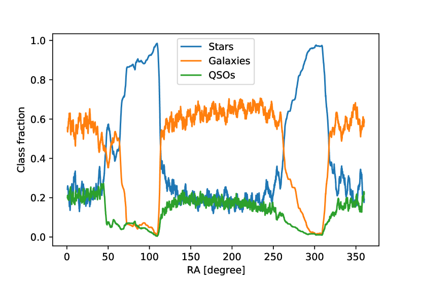
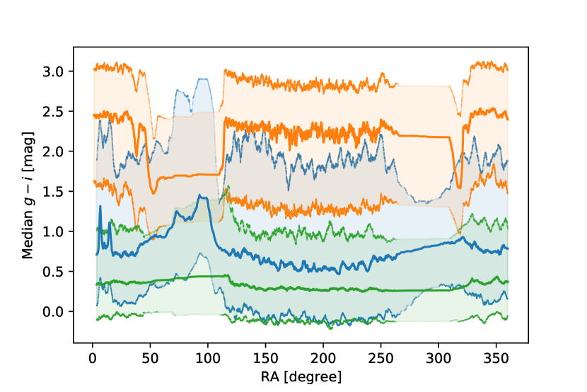
Figure 1: General characteristics of the dataset as a function of RA. Top: The fraction of sources in each of the three classes, versus RA. Bottom: The median $g-i$ colour of each class versus RA. The shaded areas show the $\pm 1\,\sigma$ range in $g-i$ for each of the three classes. In both cases, each data point represents a rolling window with a length of 1000 objects, and a step size of 1 object.

Table 1: Hyperparameters used to train the classification models. Parameters not listed here kept their default values.

Learning algorithm	Hyperparameter	Value
RandomForest	n_estimators	100
	max_depth	4
XGBoost	n_estimators	300
	max_depth	4
	tree_method	hist
	eval_metric	map
LightGBM	n_estimators	1000
	max_depth	10
	learning_rate	0.01
	colsample_bytree	0.9
	subsample	0.8

5 Model performance prediction

5.1 Model training

Models were generated using three different machine learning algorithms: the popular RandomForestClassifier method (Breiman, 2001) from the Scikit-Learn package (Pedregosa et al., 2011), and the gradient-boosting decision tree methods XGBoostClassifier (Chen & Guestrin, 2016), and LightGBMClassfier (Ke et al., 2017).

Since objective of this study is to explore the application of CBPE, rather than to identify optimal learning algorithms or hyperparameters for the selection of quasars, the most important hyperparameters were tuned manually and non-exhaustively, with the objective of producing classification models that are of an acceptably high-quality. A summary of the hyperparameters used for model training is given in Table  1.

The models were trained on 1/40 of the sources in the range $150<{\rm RA}<200$ deg. Sources used for model training were not used at any subsequent stage in the workflow.

5.2 Probability calibration

The aim of calibration is to derive and apply a transformation to class probabilities such that the transformed values correspond to the true probability of belonging to the class in question. For instance, objects assigned a class probability of 0.80 should have an 80 per cent probability of belonging to class 1. However, class probabilities produced by many classifiers are biased and poorly calibrated. Thus, as discussed in $\S$3.2, class probabilities must be calibrated before the CBPE is applied.

While there are various different methods to calibrate class probabilities (see, e.g., Niculescu-Mizil & Caruana, 2005; Kull et al., 2017), we have used the isotonic regression method, which is appropriate for relatively large datasets (≳1000 examples). This method fits a non-parametric, isotonic regressor, which yields a step wise non-decreasing function.

In the interest of simplicity and reproducibility, we have used the Scikit-Learn function CalibratedClassifierCV, which produces a calibration transformation simultaneously with the training of the classifier, using 5-fold cross-validation. Note that the same samples cannot be used to train the classifier and compute the calibration transform.

5.3 Results

For each source in the dataset that was not used for model training, the binary class and the class probability were predicted, using each of the three models. The F1-score versus RA is shown in Fig. 2 (solid blue line). The RA range from which the training sample was drawn is highlighted with cyan shading.

All three models show roughtly similar behaviour of the F1-score with respect to RA: the F1-score remains near to $\sim$0.8 over most of the RA range, but drops dramatically to $\sim 0.2$ near to ${\rm RA}\sim 90$ deg and ${\rm RA}\sim 310$ deg. Clearly, the population shifts seen in Fig. 1 have resulted in decreased classification performance in RA ranges where the number of stars is high relative to galaxies and QSOs.

Next, we apply the CBPE methodology as outlined in $\S$3 to the predictions from the classifier models. The resulting F1-score estimates are shown by the orange dashed lines in Fig. 2. The estimated score follows the measured score relatively well, with $R^{2}$-scores of 0.92, 0.76, 0.74, and MAFE scores of 0.12, 0.11, 0.12, for the RandomForestClassifier, XGBoostClassifier, and LightGBMClassifier cases, respectively. Interestingly, the CBPE method is able to predict the dramatically low F1-scores at ${\rm RA}\sim 100$ and ${\rm RA}\sim 300$ deg, but also predicts the shallow gradient in the F1-score in the range $125<{\rm RA}<250$ deg, and many of the small fluctuations.

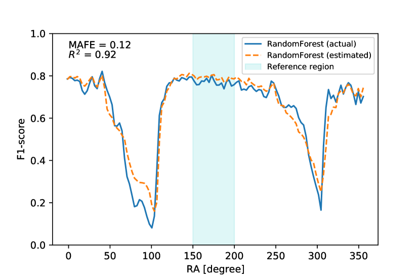
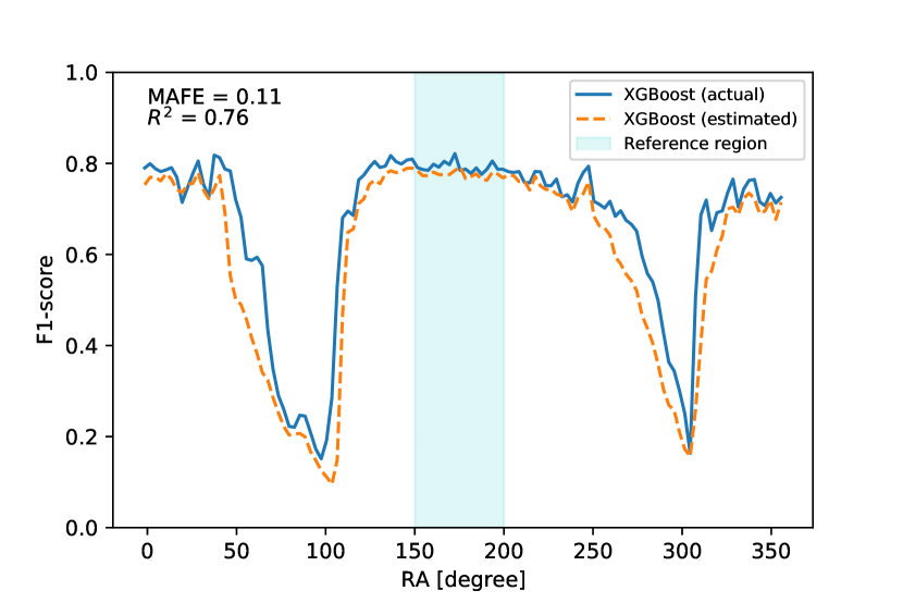
Figure 2: General characteristics of the dataset as a function of RA. Top: Estimated and actual F1-scores versus RA, for the RandomForest model. Middle: The same, but for the XGBoost model. Bottom: The same, but for the LghtGBM model. The metrics are calculated in a rolling window of length 1001 objects, with results from each window plotted at the RA value that corresponds to the central element of the bin.

6 Discussion and conclusions

We have introduced the NannyML CBPE method for the estimation of machine learning model performance in the absence of ground-truth labels. We have demonstrated that CBPE is able to predict population shift-driven changes in the performance of machine-learning models, using the selection of QSOs from SDSS photometry as an example use-case.

A number of interesting implications arise from this study. Among them is the potentially game-changing possibility to predict the classification performance of a model in the absence of ground-truth labels, even in the presence of substantial population shifts between the training and test sets. Depending on the experimental set-up employed, the application of CBPE should allow model-selection to be performed such that models (or hyperparameters) can be chosen to maximise the expected performance in unlabelled (test) data, in contrast to the traditional paradigm where performance is optimized using labelled validation data.

Another potentially fruitful use-case we envisage is the detection of population shifts in large astronomical datasets, and quantification of their impact on classification metrics (e.g., Fig. 2). We also argue that such analyses may be useful when planning wide-field surveys in which machine learning classifiers are expected to be used. For example, models trained on different deep, pencil-beam surveys might be evaluated on their performance over a wider survey area using CBPE, in order to select the model (or training sample) that is estimated to provide the highest quality result for a desired classification objective.

While the CBPE method has proven useful to predict changes in model performance under population shift, it is important to note that under concept drift, where changes occurs in the mapping between the features and the target, the performance estimates may be less accurate.

Finally, we acknowledge that the work presented in this Letter represents a restricted subset of the possible use-cases of the CBPE method in the field of astronomical source classification. A more detailed analysis and application to a wider range of classification problems is beyond the scope of this Letter, and will be the subject of a future paper.

Data Availability

The Python and SQL scripts used in this study are publicly available at https://github.com/humphrey-and-the-machine/f1_prediction.

The data were collected from the SDSS SkyServer / SciServer / CASJobs portal at https://skyserver.sdss.org/casjobs/. A CSV file containing the dataset used has been made available online, hosted by MNRAS.

References

- Angelopoulos & Bates (2022) Angelopoulos, A. N., Bates, S. 2022, ArXiv e-prints, ArXiv:2107.07511
- Arnouts et al. (1999) Arnouts, S., Cristiani, S., Moscardini, L., et al. 1999, MNRAS, 310, 540
- Bai et al. (2019) Bai, Y., Liu, J., Wang, S., et al. 2019, AJ, 157, 9
- Bayram et al. (2022) Bayram, F., Ahmed, B. S., Kassler, A. 2022, ArViv e-prints, ArXiv:2203:11070
- Bennett et al. (2022) Bennett, M., Balusu, J., Hayes, K., Kleczyk, E. J. 2022, ArXiv e-prints, ArXiv:2204.10227
- Bisigello et al. (2020) Bisigello, L., Kuchner, U., Conselice, C. J., et al. 2020, MNRAS, 494, 2337 (B20)
- Bolzonella, Miralles, & Pelló (2000) Bolzonella, M., Miralles, J.-M., & Pelló, R. 2000, A&A, 363, 476
- Bowles et al. (2021) Bowles, M., Scaife, A. M. M., Porter, F., Tang, H., & Bastien, D. J. 2021, MNRAS, 501, 4579
- Breiman (2001) Breiman, L. 2001, Mach. Learn., 45, 1
- Bretonnière et al. (2021) Bretonnière, H., Boucaud, A., & Huertas-Company, M. 2021, ArXiv e-prints, ArXiv:2111.15455
- Cavuoti et al. (2014) Cavuoti, S., Brescia, M., D’Abrusco, R., Longo, G., & Paolillo, M. 2014, MNRAS, 437, 968
- Chen & Guestrin (2016) Chen, T., Guestrin, C., 2016, ArXiv e-prints, ArXiv:1603.02754v3
- Clarke et al. (2020) Clarke, A. O., Scaife, A. M. M., Greenhalgh, R., & Griguta, V. 2020, A&A, 639, A84
- Cunha & Humphrey (2022) Cunha, P. A. C. & Humphrey, A. 2022, ArXiv e-prints, ArXiv:2204.02080. doi:10.1051/0004-6361/202243135
- da Cunha et al. (2008) da Cunha, E., Charlot, S., & Elbaz, D. 2008, MNRAS, 388, 1595
- Daddi et al. (2004) Daddi, E., Cimatti, A., Renzini, A., et al. 2004, ApJ, 617, 746
- Dice (1945) Dice, L. R., 1945, Ecology, 26(3), 297
- Dieleman, Willett, & Dambre (2015) Dieleman, S., Willett, K. W., & Dambre, J. 2015, MNRAS, 450, 1441
- Domínguez Sánchez et al. (2018) Domínguez Sánchez, H., Huertas-Company, M., Bernardi, M., et al. 2018, MNRAS, 476, 3661
- El-Hay & Yanover (2022) El-Hay, T., Yanover, C., Proceedings of the Conference on Health, Inference, and Learning. PMLR, 2022, p. 48-62. ArXiv e-prints, ArXiv:2202.13683
- Euclid Collaboration: Humphrey et al. (2022) Euclid Collaboration, Humphrey, A., et al. 2022, A&A, accepted, ArXiv e-prints, ArXiv:2209.13074
- Euclid Collaboration: Scaramella et al. (2021) Euclid Collaboration, Scaramella, R., Amiaux, J., et al. 2022, A&A, 662, A112
- Fawcett (2006) Fawcett, T., Pattern Recognition Letters 27, 2006, 861–874
- Gomes & Papaderos (2017) Gomes, J. M., & Papaderos, P. 2017, A&A, 603, A63
- Gunn et al. (1998) Gunn, J. E., Carr, M., Rockosi, C., et al. 1998, AJ, 116, 3040
- Haro (1956) Haro, G. 1956, Boletin de los Observatorios Tonantzintla y Tacubaya, 2, 8
- Harris et al. (2020) Harris, C. R., Millman, K. J., van der Walt, S. J., et al. 2020, Nature, 585, 357
- Huertas-Company et al. (2015) Huertas-Company, M., Gravet, R., Cabrera-Vives, G., et al. 2015, ApJS, 221, 8
- Ilbert et al. (2006) Ilbert, O., Arnouts, S., McCracken, H. J., et al. 2006, A&A, 457, 841
- Ivezić et al. (2019) Ivezić, Ž., Kahn, S. M., Tyson, J. A., et al. 2019, ApJ, 873, 111
- Jiang et al. (2018) Jiang, H., Kim, B., Guan, M. Y., Gupta, M., 2018, 32nd Conference on Neural Information Processing Systems (NIPS 2018), Montréal, Canada. ArXiv e-prints, ArXiv:1805.11783
- Ke et al. (2017) Ke, G., Meng, Q., Finley, T., Wang, T., Chen, W., Ma, W., Ye, Q., and Liu, T.-Y., 2017, LightGBM: A Highly Efficient Gradient Boosting Decision Tree, in Advances in Neural Information Processing Systems, vol. 30, 3146
- Kull et al. (2017) Kull, M., Silva Filho, T. M., Flach, P., 2017, Electron. J. Statist., 11 (2), 5052-5080
- Laigle et al. (2016) Laigle, C., McCracken, H. J., Ilbert, O., et al. 2016, ApJS, 224, 24
- Laureijs et al. (2011) Laureijs, R., Amiaux, J., Arduini, S., et al. 2011, ArXiv e-prints [\eprint[arXiv]1110.3193]
- Leja, Tacchella, & Conroy (2019) Leja, J., Tacchella, S., & Conroy, C. 2019, ApJ, 880, L9
- Malinin et al. (2020) Malinin, A., Prokhorenkova, L., Ustimenko, A. 2020, ArXiv e-prints, ArViv:2006.10562
- McKinney (2010) McKinney, w., 2010, Data Structures for Statistical Computing in Python, in Proceedings of the 9th Python in Science Conference, pp 51
- Niculescu-Mizil & Caruana (2005) Niculescu-Mizil, A., Caruana, R., 2005, in Proceedings of the 22nd International Conference on Machine Learning, Bonn, Germany
- Nolte et al. (2019) Nolte, A., Wang, L., Bilicki, M., Holwerda, B., & Biehl, M. 2019, arXiv e-prints, ArXiv:1903.07749
- Pedregosa et al. (2011) Pedregosa, F., et al., 2011, Journal of Machine Learning Research, 12, 2825
- Rocklin (2015) Rocklin, M., 2015, Dask: Parallel Computation with Blocked Algorithms and Task Scheduling, in Proceedings of the 14th Python in Science Conference, pp 130
- Scoville et al. (2007) Scoville, N., Aussel, H., Brusa, M., et al. 2007, ApJS, 172, 1
- Singh Sethi & Kantardzic (2017) Singh Sethi, T., Kantardzica, M. 2017, ArXiv eprints, ArXiv:1704.00023
- Sørensen (1948) Sørensen T. 1948, Kongelige Danske Videnskabernes Selskab, 5(4): 1
- Tuccillo et al. (2018) Tuccillo, D., Huertas-Company, M., Decencière, E., et al. 2018, MNRAS, 475, 894
- Vilalta et al. (2019) Vilalta, R., Dhar Gupta, K., Boumber, D., et al. 2019, PASP, 131, 108008
- Virtanen et al. (2020) Virtanen, P., Gommers, R., Oliphant, T. E., et al. 2020, Nature Methods, 17, 261
- White et al. (2019) White, C., Neiswanger, W., Savani, Y. 2019, 4th workshop on Bayesian Deep Learning (NeurIPS 2019), Vancouver, Canada. E-print: http://bayesiandeeplearning.org/2019/papers/26.pdf