Improving Power Spectral Estimation using Multitapering:
Precise asteroseismic modeling of stars, exoplanets, and beyond

Abstract

Asteroseismic time-series data have imprints of stellar oscillation modes, whose detection and characterization through time-series analysis allows us to probe stellar interiors physics. Such analyses usually occur in the Fourier domain by computing the Lomb-Scargle (LS) periodogram, an estimator of the power spectrum underlying unevenly-sampled time-series data. However, the LS periodogram suffers from the statistical problems of (1) inconsistency (or noise) and (2) bias due to high spectral leakage. In addition, it is designed to detect strictly periodic signals but is unsuitable for non-sinusoidal periodic or quasi-periodic signals. Here, we develop a multitaper spectral estimation method that tackles the inconsistency and bias problems of the LS periodogram. We combine this multitaper method with the Non-Uniform Fast Fourier Transform (mtNUFFT) to more precisely estimate the frequencies of asteroseismic signals that are non-sinusoidal periodic (e.g., exoplanet transits) or quasi-periodic (e.g., pressure modes). We illustrate this using a simulated and the Kepler-91 red giant light curve. Particularly, we detect the Kepler-91b exoplanet and precisely estimate its period, $6.246\pm 0.002$ days, in the frequency domain using the multitaper F-test alone. We also integrate mtNUFFT into the PBjam package to obtain a Kepler-91 age estimate of $3.96\pm 0.48$ Gyr. This $36$% improvement in age precision relative to the $4.27\pm 0.75$ Gyr APOKASC-2 (uncorrected) estimate illustrates that mtNUFFT has promising implications for Galactic archaeology, in addition to stellar interiors and exoplanet studies. Our frequency analysis method generally applies to time-domain astronomy and is implemented in the public Python package tapify, available at https://github.com/aaryapatil/tapify.

1 Introduction

Modern advances in the theory of stellar structure and evolution are driven by high-precision photometric observations of stars over time using space-based telescopes such as the MOST (Walker et al., 2003), CoRoT (Baglin et al., 2009; Auvergne et al., 2009), Kepler (Borucki et al., 2010; Koch et al., 2010) (and K2), BRITE (Weiss et al., 2014), TESS (Ricker et al., 2014), and the upcoming PLATO mission (Rauer et al., 2014) (e.g., Buzasi et al., 2000; Michel et al., 2008; Miglio et al., 2009; Aerts et al., 2010; De Ridder et al., 2009; Degroote et al., 2010; Chaplin et al., 2011; Li et al., 2020). Analyses of these observations in the Fourier domain exhibit the frequencies at which stars oscillate. By studying these frequencies, asteroseismology provides a unique pathway to investigate the deep interiors of stars and the physical mechanisms that drive oscillations.

To obtain Fourier domain representations of stellar oscillations, one estimates the power spectrum from the light curve, or time-series, data. The features in the power spectrum across frequencies are associated with different physical phenomena, and these features in turn depend on the type of pulsating star (refer to the pulsation HR diagram in Aerts et al., 2010, chapter 2). In the case of solar-like oscillators, we can observe the following spectral features (García & Ballot, 2019):

1. rotational modulation peaks and harmonics,

2. transitory exoplanet peaks and harmonics,

3. continuum resulting from granulation in the outer convective zones,

4. pressure (p) mode envelope of resonant oscillations,

5. and a photon noise level.

Together, these features provide the most stringent constraints on stellar structure models while also allowing precise exoplanet detection.

Solar-like oscillations are expected in stars with convective envelopes. We thus observe them in low-mass main sequence ($M\lesssim 1.5M_{\odot}$), subgiant branch, and G-K red giant stars (Hekker et al., 2011; White et al., 2011), which form the most abundant type of oscillators. A set of acoustic p-modes or standing sound waves probe the turbulent outer layers of these oscillators (refer to point 4). In theory, these modes are damped stochastically excited harmonic oscillations, represented by a sequence of quasi-evenly spaced Lorentzian profiles in frequency space (Aerts et al., 2010). We can characterize these modes in power spectra to estimate stellar masses and radii using either the model-independent or model-dependent approach. The model-independent approach uses simple scaling relations with the Sun (Kjeldsen & Bedding, 1995) and is efficient as compared to detailed stellar modeling. However, its accuracy and precision is limited by the uncertainty on $\Delta\nu$ and $\nu_{\mathrm{max}}$ estimates and the approximations underlying the scaling relations. The stellar model-dependent approach provides more accurate and precise estimates, with the frequency estimates being the major source of uncertainty.

In this paper, we target the reduction of uncertainty on $\Delta\nu$ and $\nu_{\mathrm{max}}$ as well as individual p-mode frequencies as a way to provide stringent constraints on stellar masses, radii, and therefore ages, beyond the ${\sim}3\%$, ${\sim}1\%$, and ${\sim}10\%$ precision of current methods (Bellinger et al., 2019). To reduce these uncertainties, we present a new frequency analysis method, the multitaper NUFFT (mtNUFFT) periodogram, that mitigates the statistical issues of the standard Lomb-Scargle (LS) periodogram to better estimate power spectra (detailed in 1.1). Our focus is mainly on precise estimation of red giant ages as they help characterize ensembles of stellar populations out to large distances, thereby enabling Galactic archaeological studies.

In addition to inference of stellar properties, light curve data embed information of exoplanets orbiting stars (refer to point 2). In fact, many of the space-based telescopes delivering asteroseismic data were designed for the detection of planetary transits, especially those undetectable from the ground due to their small radii (Marcy et al., 2005; Kunimoto & Matthews, 2020). Precise estimation of the fundamental properties of exoplanets and their stellar hosts such as mass, radius, and age along with orbital parameters can help resolve outstanding questions on the formation and evolution of planetary systems.

Exoplanet transits are periodic in nature, but have highly non-sinusoidal shapes and low signal-to-noise (SNR) ratios. Therefore, specialized methods that identify such signals in time-series were introduced for exoplanet detection (e.g., Lafler & Kinman, 1965; Stellingwerf, 1978), rather than the LS periodogram that is optimized for sinusoidal signals. The widely used Box periodogram (Kovács et al., 2002) is one such method that performs least squares fitting of step functions to folded time-series. Gaussian process modeling of stellar activity and transiting exoplanets is currently gaining popularity as a more precise approach but remains computationally expensive (Aigrain et al., 2015; Faria et al., 2016; Foreman-Mackey et al., 2017; Serrano et al., 2018; Barros et al., 2020).

We target the automatic detection of transitory exoplanets and uncertainty reduction of their period estimates. In addition to power spectral densities, mtNUFFT offers phase information, which when combined with the multitaper F-test (Thomson, 1982), detects periodic signals hidden in noise. Extraction and characterization of these periodic signals allows us to detect transitory exoplanets and two types of asteroseismic modes: coherent gravity (g) modes and undamped modes with quasi-infinite lifetimes. While this paper primarily focuses on solar-like oscillators, whose spectra are dominated by p-modes, we will show how our methods are applicable to other types of pulsating stars exhibiting either g or undamped modes.

1.1 Statistical Background

In order to obtain high-precision frequency estimates of p-modes or exoplanet transits using light curve data, we need a statistically reliable estimator of the power spectrum. Many non-parametric spectral estimators have been developed for data sampled regularly in time and their statistical properties are well established in the literature. The oldest of these, the classical periodogram (Schuster, 1898), is commonly used in science and engineering but is inconsistent and biased. The inconsistency comes from non-zero variance (or noise) of the estimator and bias from high spectral leakage, i.e., the leakage of power from one frequency to another. While there exists no unbiased estimator of the spectrum underlying a discrete time-series sampled over a finite time interval, estimators that taper the data significantly reduce and control bias (Brillinger, 1981). However, reduced bias is at the expense of reduced variance efficiency and loss of information. Instead of using just one taper, Thomson (1982) use multiple orthogonal tapers called Discrete Prolate Spheroidal Sequences (DPSS; Slepian, 1978) to obtain an averaged estimate of a number of single-tapered estimates. This method treats both the bias and inconsistency problems, minimizes loss of information, and outperforms un-tapered and single-tapered non-parametric estimates (with or without smoothing) (Park et al., 1987; Bronez, 1992; Riedel et al., 1994; Stoica & Sundin, 1999; Prieto et al., 2007; Thomson & Haley, 2014) as well as parametric estimates (Lees & Park, 1995). It is very popular in different fields of science and engineering; particularly interesting applications are those in geophysics, solar physics, and helioseismology since they have many similarities with asteroseismology (for e.g. Park et al., 1987; Thomson et al., 1996; Thomson & Vernon, 2015a, b; Chave, 2019; Chave et al., 2020; Mann et al., 2021).

Time-series data in astronomy are often dependent on observational factors resulting in irregular sampling. This is true for modern space-based asteroseismic data, e.g., Kepler observations (Borucki et al., 2010; Koch et al., 2010) are over Q0-Q16 quarters, each of ${\approx}3$ months duration, with data downlinks that result in gaps as well as slight uneven-sampling due to conversion of evenly-sampled time stamps to Barycentric Julian Date. While one can interpolate such irregularly-sampled time-series data to a mesh of regular times (e.g. García et al., 2014) and use estimators based on the assumption of even sampling, Lepage & Thomson (2009) and Springford et al. (2020) demonstrate that interpolation leads to spectral leakage by introducing power from the method and thus has undesirable effects on spectral estimates. Instead, the Lomb-Scargle (LS) periodogram (Lomb, 1976; Scargle, 1982) is widely regarded as a standard solution to the spectrum estimation problem for irregular sampling and is particularly popular in astronomy. However, it suffers from the same statistical issues as the classical periodogram and its spectral leakage worsens with increased irregularity of the time samples (VanderPlas, 2018). We thus develop the mtNUFFT periodogram that extends the Thomson multitaper spectral estimate to irregular sampling and improves upon the noise and spectral leakage properties of the LS periodogram. This new periodogram is particularly favourable for detecting quasi-periodic signals (e.g., p-modes) as well as periodic non-sinusoidal-shaped signals (e.g., exoplanet transits) in space-based light curves, and is an extension of the mtLS periodogram developed in Springford et al. (2020).

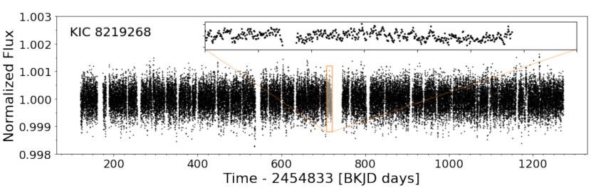
Figure 1: Photometric time series of Kepler red giant star-91. The inset shows a zoom-in plot of the time-series from 708 to 722 days, highlighting that the time sampling is uneven and that long gaps are present.

1.2 Overview

The outline of the paper is as follows. Section 2 motivates the use of multitaper spectral estimation in asteroseismology given its statistical background, and introduces our multitaper spectral estimation method, the mtNUFFT periodogram. This section presents pedagogy for readers new to time-series analysis. We thus direct the experienced reader to Section 2.2 that presents our new frequency analysis method and its novelty compared to the state-of-the-art. To demonstrate the advantageous statistical properties of our method, we apply it to an example Kepler time-series of a solar-like oscillator: the red giant KIC 8219268 (or Kepler-91). We then simulate a light curve of a solar-like oscillator to show that our method allows precise characterization of p-modes. In Section 3, we focus on harmonic analysis for the detection of transitory exoplanets in asteroseismic time-series data. We extend the Thomson F-test (Thomson, 1982) to our mtNUFFT periodogram and show that it can automatically detect the Kepler-91b exoplanet signal (Batalha et al., 2013) in the Kepler-91 time-series and precisely estimate its orbital period. Section 4 illustrates the improvement in age estimation provided by mtNUFFT as compared to the LS periodogram using our Kepler-91 case study example. We use the PBjam peakbagging Python package to perform this comparison. Finally, we compare our results with those from the APOKASC-2 catalog (Pinsonneault et al., 2018). We discuss the advantages and improvements of our methods for asteroseismology and time-domain astronomy in Section 5. The concluding Section 6 summarizes the paper and its key takeaways.

Appendix A discusses tapify, a Python package we develop for multitaper spectral analysis, and provides a workable example. Appendix B provides recommendations for choosing (or tuning) the parameters of the mtNUFFT periodogram and other practical considerations when using multitapering for time-series analysis.

2 Spectral Estimation in Asteroseismology

An important statistical problem in asteroseismology is the detection of oscillation signals given discrete time-series data over a finite time interval. To demonstrate the challenges underlying this problem, in this section we focus on analyzing a Kepler photometric time-series (light curve) KIC 8219268 for a red giant, Kepler-91, shown in Figure 1. This analysis draws inspiration from and builds upon the example in Springford et al. (2020). We refer the reader to this paper for information on the pre-processing of the Kepler-91 light curve.

Figure 1 shows that the time stamps of the Kepler light curve are unevenly spaced and long time gaps are present (see also Kallinger et al., 2014). This leads us to the first time-series analysis problem in asteroseismology, irregular sampling, which we discuss and tackle in Section 2.1. Particularly, we highlight the shortcomings of the LS periodogram in Section 2.1.1, and propose a solution in Section 2.1.2.

Figure 3 illustrates the statistical problems of bias and inconsistency. These problems have not received much attention until recently, even though they can lead to spurious peaks in the spectral estimates and cause false mode detection in asteroseismic analyses. Section 2.2 discusses this problem. The general solution to this problem is the Thomson multitaper approach (Thomson, 1982), which we discuss in Section 2.2.1. While this approach was originally developed for regularly-sampled (i.e. evenly-sampled) time-series (refer to Section 2.2.2), a multitaper version of the LS periodogram was recently developed for irregular (i.e. uneven) sampling (Springford et al., 2020). The multitaper LS (mtLS) periodogram is the same as the Thomson multitaper in the limit of regular sampling and exhibits less spectral leakage and variance compared to the un-tapered version. We discuss the advantages mtLS offers to asteroseismic mode extraction in Section 2.2.3. Finally, we introduce mtNUFFT, the extension of mtLS, in Section 2.2.4 and show that it is particularly favourable for detecting quasi-periodic modes (e.g., p-modes) in quasi-regularly sampled space-based light curves.

Table 1: Mathematical Notation

Symbol	Description
$n$	sample index in time-series
$\mathbf{x}=\{x_{n}\}$	vector of evenly or unevenly-sampled time-series
$\Delta t$	sampling interval for evenly-sampled $\mathbf{x}$
$\mathbf{t}=\{t_{n}\}$	vector of timestamps for unevenly-sampled $\mathbf{x}$
$N$	sample size of $\mathbf{x}$
$T$	time duration of $\mathbf{x}$
$\overline{\Delta t}$	mean sampling interval for unevenly-sampled $\mathbf{x}$
$M$	zero-padded length of $\mathbf{x}$
$f$	frequency
$f_{\mathrm{Nq}}$	Nyquist frequency
$\tau_{\mathrm{LS}}$	time-offset of LS periodogram
$\mathcal{FT}_{\mathbf{x}}(f)$	Fourier transform of $\mathbf{x}$
$S(f)$	true spectrum underlying $\mathbf{x}$
$\hat{S}^{(\mathrm{type})}(f)$	spectral estimate of a given type
$W,NW$	bandwidth, time-bandwidth product
$K$	number of tapers $\leq 2NW-1$
$k$	index (order) of taper
$\mathbf{v}(N,W)$	$K\times N$ matrix of evenly-sampled tapers [$v_{k,n}$]
$\mathbf{v}^{\star}(N,W)$	$K\times N$ matrix of tapers interpolated to $\mathbf{t}$
$\lambda_{k}(N,W)$	eigenvalue of taper $k$
$U_{k}(N,W;f)$	Fourier transform of taper $k$ (eigenfunction)
$y_{k}(f)$	eigencoefficient of taper $\mathbf{v}_{k}$
$\hat{S}_{k}(f)$	single-tapered spectral estimate of order $k$
$d_{k}(f)$	adaptive weight of $\hat{S}_{k}(f)$
$\hat{S}^{(\mathrm{mt})}(f)$	multitaper spectral estimate
$\hat{S}^{(\mathrm{mt})}_{\setminus j}(f)$	delete-one [$\hat{S}_{j}(f)$] multitaper spectral estimate
$M(\bm{\theta},\nu)$	Model spectrum [parameters $\bm{\theta}$ and frequency $\nu$]
$\hat{\mu}(f)$	amplitude estimate of periodic signal at $f$
$F(f)$	F-statistic for multitaper F-test
$\hat{f}_{0}$	maximum F-statistic frequency
$\mathrm{Var}\{\hat{f}_{0}\}$	F-test variance
$f_{p},\hat{f}_{p}$	strictly periodic signal of interest and estimate

Note. — We use the above mathematical notation in this paper. Note that we use $\nu$ for model frequency (and $\nu_{nl}$ for asteroseismic modes) instead of $f$ to distinguish between data and theory.

2.1 Sampling of Time-Series Data

The irregularity of Kepler time-series and other space-based observations makes spectral estimation in asteroseismology challenging. The statistical behavior of spectral estimators in the regularly-sampled case is well understood, making detection of periodic signals in time-series reliable. One such non-parametric estimator with the simplest statistical behaviour is the classical periodogram (Schuster, 1898). This estimator is commonly used and is given by

$$\hat{S}^{(\mathrm{P})}(f)=\frac{1}{N}\left|\sum_{n=0}^{N-1}x_{n}e^{-i2\pi fn}\right|^{2}$$ (1)

where $\mathbf{x}=\{x_{n}\mid n=0,...,N-1\}$ is a zero-mean (strong or weak) stationary time-series with sampling $\Delta t=1$. If we denote the discrete Fourier Transform (DFT) of $\mathbf{x}$ as $\mathcal{FT}_{\mathbf{x}}(f)$, then Equation (1) becomes

$$\hat{S}^{(\mathrm{P})}(f)=\frac{1}{N}\left|\mathcal{FT}_{\mathbf{x}}(f)\right|^{2}.$$ (2)

By exploiting symmetries in the DFT terms, the Fast Fourier Transform (FFT) algorithm (Cooley & Tukey, 1965) can efficiently and accurately compute $\mathcal{FT}_{\mathbf{x}}(f)$ in Equation (2) at $N/2$ regularly-spaced frequencies

$$f_{n}=n/N\;\;\mathrm{for}\,n=0,1,\dotsc,\lfloor{N/2}\rfloor$$ (3)

These frequencies are equivalent to a principle frequency domain of $[-\frac{1}{2},\frac{1}{2})$, where $\frac{1}{2}$ is the largest frequency we can completely recover (without aliasing). This frequency is called the Nyquist frequency, and is given by

$$f_{\mathrm{Nq}}=\frac{1}{2\Delta t}$$ (4)

for any sampling $\Delta t$.

The FFT algorithm is orders-of magnitude faster than its “slow” counterpart. It is most efficient when $N$ is a power of 2, and hence the time-series data $\mathbf{x}$ is zero padded to length $M\geq N$, where $M$ satisfies the power of 2 condition. Zero padding by at least a factor of 2 ($M\geq 2N$) can also help circumvent circular correlations. Such a zero-padded version of FFT results in a finer frequency grid as the spacing reduces from $1/N$ to $1/M$. There are many other reasons for zero-padding, and we expand upon some of them in Section 3.

While the classical periodogram definition generalizes to irregularly-sampled time-series, its statistical behavior does not directly translate to it. Therefore, certain modifications are necessary which we explore in the following section.

2.1.1 How to Handle Irregular Sampling?

The classical periodogram in the regular sampling case has well-defined statistical properties. E.g., the periodogram of an evenly-sampled Gaussian noise process has a $\chi^{2}$ distribution with 2 degrees of freedom ($\chi_{2}^{2}$) (Schuster, 1898). This attribute allows us to analyze the presence of spurious peaks in the spectral estimates. However, the simple statistical properties of the classical periodogram do not hold in the irregular sampling case, i.e., one cannot define the periodogram distributions analytically. Scargle (1982) tackle this issue by modifying the periodogram to the Lomb-Scargle (LS) periodogram for irregular time sampling. The LS estimator is given by

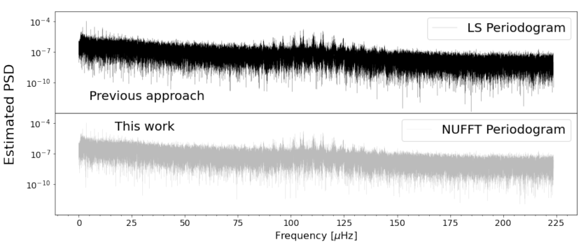
Figure 2: Comparison between the LS periodogram and the NUFFT periodogram of the Kepler-91 time-series. This illustrates that the NUFFT periodogram we introduce in Section 2.1.2 behaves similar to the LS periodogram in the case of quasi-evenly-sampled time-series with gaps.

$$\hat{S}^{(\mathrm{LS})}(f)=\frac{1}{2}\frac{\left\{\sum\limits_{n=0}^{N-1}x_{n}cos\left[2\pi f(t_{n}-\tau_{\mathrm{LS}})\right]\right\}^{2}}{\sum\limits_{n=0}^{N-1}cos^{2}\left[2\pi f(t_{n}-\tau_{\mathrm{LS}})\right]}\\ +\frac{1}{2}\frac{\left\{\sum\limits_{n=0}^{N-1}x_{n}sin\left[2\pi f(t_{n}-\tau_{\mathrm{LS}})\right]\right\}^{2}}{\sum\limits_{n=0}^{N-1}sin^{2}\left[2\pi f(t_{n}-\tau_{\mathrm{LS}})\right]}$$ (5)

where $\mathbf{x}=\{x_{n}\}$ corresponding to time stamps $\mathbf{t}=\{t_{n}\mid n=0,...,N-1\}$ is an irregularly-sampled time-series. $\tau_{\mathrm{LS}}$ is the time-offset given by

$$\tan\left(2f\tau_{\mathrm{LS}}\right)=\frac{\sum\limits_{n=0}^{N-1}sin\left(4\pi ft_{n}\right)}{\sum\limits_{n=0}^{N-1}cos\left(4\pi ft_{n}\right)}$$ (6)

that makes the periodogram invariant to time-shifts. The distribution of this modified periodogram is equivalent to the classical periodogram.

The LS periodogram was designed to detect a single periodic signal embedded in normally distributed independent noise (Scargle, 1982). It is essentially a Fourier analysis method that is statistically equivalent to performing least-squares fitting to sinusoidal waves (Lomb, 1976), which can be shown using Equation (5). We refer the reader to VanderPlas (2018) for an in-depth review of the LS periodogram estimator.

Press & Rybicki (1989) were the first to efficiently compute the LS periodogram in $\mathcal{O}(N\log{}M)$, where $M$ is the number of frequencies, using FFTs. Leroy (2012) further improve this efficiency by an order-of-magnitude using the Non-Uniform FFT (NUFFT) (refer to Keiner et al., 2009, or Section 2.1.2 for details of NUFFT). The astropy package (Astropy Collaboration et al., 2022) includes this algorithm along with several other “slow” $\mathcal{O}(NM)$ versions to compute spectral estimates on a frequency grid, $f\in[0,f_{\mathrm{Nq}}]$, with an oversampling factor of 5 (equivalent to zero-padding by $M=5N$). Here $f_{\mathrm{Nq}}$ is the average Nyquist frequency computed using $\overline{\Delta t}$ in Equation (4).

2.1.2 Periodic vs Quasi-Periodic Modes

Given the irregular time sampling of space-based light-curves such as those from Kepler, the LS periodogram is the preferred spectral estimator. However, since time gaps can be separately handled (Fodor & Stark, 2000; Smith-Boughner & Constable, 2012; Pires et al., 2015; Chave, 2019), the light-curves can be treated as quasi-evenly sampled. In this case, the statistical properties of the classical periodogram should hold to some degree. Taking advantage of this, we implement a periodogram for irregular sampling using the NUFFT (also called non-equispaced FFT) (Keiner et al., 2009; Barnett et al., 2018). Essentially, we directly generalize the classical periodogram to the irregular sampling case as

$$\hat{S}^{(\mathrm{NP})}(f)=\frac{1}{N}\left|\sum_{n=0}^{N-1}x_{n}e^{-i2\pi ft_{n}}\right|^{2}$$ (7)

and compute the non-uniform or non-equispaced DFT in the definition using the adjoint NUFFT. The principles of zero-padding apply to the adjoint NUFFT as they do to the FFT.

We can think of the NUFFT periodogram as a simpler version of the LS; instead of using the adjoint NUFFT directly to compute Equation (7), the LS uses the transform to compute the modified components in Equation (5). Thus, the NUFFT periodogram is slightly more efficient than the LS.

In addition to efficiency, we expect the NUFFT periodogram to outperform the LS periodogram at detecting quasi-periodic signals in the case of irregular sampling. The LS is tailored to strictly periodic signals hidden in white noise (Scargle, 1982), but is not ideal for analysing multiple quasi-periodic signals (e.g., p-modes) on top of red noise (or smooth background signals). P-modes have Lorentzian profiles in the frequency domain whereas background signals due to granulation and magnetic activity have a smooth low-frequency trend (Kallinger et al., 2014; Aerts, 2021); for these signals, we expect NUFFT to perform better than LS. We refer the reader to VanderPlas (2018) for more details on the shortcomings of the LS periodogram.

Figure 2 compares the NUFFT periodogram with the LS periodogram for the Kepler-91 time-series. We use the adjoint (type 1) NUFFT from the FINUFFT package (Barnett et al., 2019; Barnett, 2021) and the default astropy LS implementation for computing the two periodograms. Both have a frequency grid with an oversampling factor of 5. A comparison between the two spectral estimates shows that, excluding some random variations across the two periodograms that follow their distribution properties, the two estimates agree with each other. They are both able to extract the comb-like p-mode structure around the frequency of 115 $\mu$Hz. However, we do expect subtle differences in the mode frequency estimates of the two periodograms, which scale with the irregularity of the time-samples. In theory, the LS works better for highly irregular or random time samples, whereas the NUFFT works better for quasi-even sampling (and both would be the same for even sampling).

There are slight differences in the amplitudes of the low frequency signals on top of the granulation and magnetic background in Figure 2, which could be due to differences in the way the two estimators detect periodic components as discussed above. However, we show in Section 3 that the phase information that NUFFT offers can be leveraged to better extract purely periodic signals in addition to the quasi-periodic signals and smooth backgrounds it readily detects. Thus, the modified NUFFT periodogram we propose precisely detects different types of modes and background signals in asteroseismology.

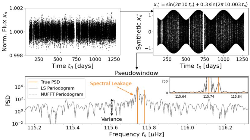
Figure 3: Spectral analysis of the pseudowindow generated using the irregular sampling times of the Kepler-91 light curve shown in the top left panel. The top right panel displays the synthetic light curve composed of two sinusoidal signals sampled at the times $t_{n}$ of the Kepler-91 series. The bottom panel shows a zoomed-in version of the LS (black) and NUFFT (grey) periodograms of the synthetic light curve $x^{\star}(t_{n})$ to focus on the two sinusoidal signals injected into the time-series and visualize their inconsistency and spectral leakage compared to the true PSD in orange. Note that the bottom panel is in log scale, whereas its inset is in linear scale to better view the difference between the signals and the noise.

2.2 Statistical issues with the Periodogram

While the LS periodogram solves the problem of detecting a periodic signal in irregularly-sampled data and has simplistic statistical behaviour, it suffers from the problems of inconsistency and spectral leakage that are inherent to the analysis of a finite, discrete, and noisy time-series. They are as follows:

1. Inconsistency: An inconsistent estimator is one whose variance does not tend to zero as the sample size $N\to\infty$. The variance of the estimator is high even for data with high SNR and it does not reduce with increasing $N$. For e.g., the LS periodogram of a Gaussian noise process is exponentially ($\chi^{2}_{2}$) distributed with large variance. The variance also does not reduce as $N$ increases because the number of frequencies recovered by the estimate, given by $N/2$ as in Equation (3), proportionally increases.

2. Spectral leakage: Spectral leakage refers to the leakage of power at a given frequency to other frequencies. Several sources of leakage are known to affect spectral estimates. The finite time interval of time-series observations represents a rectangular window and leads to side lobes that cause leakage to nearby frequencies. In contrast, the discreteness of the time-series causes leakage to distant frequencies. Thus, leakage can lead to badly biased spectral estimates, especially when the sample size $N$ is small.

The classical periodogram faces the same issues albeit with a smaller degree of spectral leakage. We can analytically define the spectral window function (the frequency response of a time-domain window) for evenly-sampled data which completely describes the spectral leakage properties of the periodogram. In contrast, the spectral leakage of the LS periodogram does not have a simple analytical definition. It depends on the exact time-sampling structure, is frequency-specific, and is often worse than that of the periodogram.

We can visualize the spectral leakage properties of the LS periodogram by investigating the pseudowindow in Figure 3. A pseudowindow is the response of a spectral estimator to a pure sinusoidal signal of a given frequency with the same sampling as the time-series of interest. It helps examine the spectral leakage for a given sampling. We create two sinusoids $x^{\star}(t)=\sin(2\pi 10t)+0.3\sin(2\pi 10.003t)$ of frequencies $10$ and $10.003$ cycles/day (or $115.74$ and $115.78\mu$Hz) respectively and sample them at the times of the Kepler-91 series. The bottom panel of Figure 3 displays the true Power Spectral Density (PSD) of the synthetic light curve that is given by two delta functions at the frequencies of the sinusoids with heights equal to the sinusoid amplitudes. It illustrates the spectral leakage and variance of the LS estimate. Particularly, we see that the leakage of power from the two sinusoid frequencies results in spurious peaks in their vicinity. These peaks can lead to false discoveries when analyzing Kepler time-series (refer to VanderPlas (2018) for more details). We expect that the NUFFT periodogram has similar spectral leakage properties (especially for strictly periodic signals) since it is a direct generalization of the classical periodogram to irregular sampling. Figure 3 also shows the pseudowindow for NUFFT to demonstrate this.

2.2.1 How does the Multitaper Spectral Estimate help?

As discussed earlier, the motive in Scargle (1982) was to detect a strictly periodic component embedded in a white noise process. However, the spectral leakage properties of the LS estimator are poor, especially if the underlying spectrum is not of the type envisioned. In this case, Scargle (1982) suggests computing the LS periodogram on tapered time-series data to mitigate spectral leakage (Brillinger, 1981).

Tapering a time-series reduces spectral leakage, but there is a tradeoff between bias control and variance reduction (or efficiency). Instead of using a single-tapered spectral estimate, Thomson (1982) develop the multitaper estimate which uses DPSS (Slepian, 1978) as tapers to optimally reduce spectral leakage along with variance. The tapers are orthogonal to each other and hence provide independent estimates of the spectrum, which are averaged to minimize variance. Thus, both spectral leakage and inconsistency are tackled by the multitaper estimate, and this makes it an improvement over the classical periodogram in the even sampling case as well as the LS periodogram in the uneven sampling case. While the multitaper estimate was originally developed for a regularly-sampled time-series, a multitaper version of the LS periodogram was recently developed for irregular sampling (Springford et al., 2020). We discuss the multitaper versions for regular and irregular sampling in Sections 2.2.2 and 2.2.3, and introduce our new mtNUFFT method in Section 2.2.4.

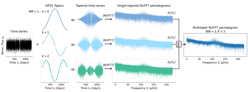
Figure 4: Schematic diagram illustrating the estimation of the mtNUFFT periodogram described in Section 2.2.4. The left panel shows the Kepler-91 time-series for which we compute the spectral estimate. The middle panels show three DPSS or Slepian tapers with time-bandwidth product $NW=2$ and order $k=0,1,2$ (number of tapers $K=2NW-1$), their corresponding tapered time-series, and the single-tapered NUFFT periodogram. The rightmost panel shows the multi-tapered NUFFT or mtNUFFT periodogram that is constructed by averaging the three single-tapered estimates with adaptive weights $d_{k}(f)$.

2.2.2 Multitaper Spectral Estimate for Regular Sampling

Thomson (1982) develop the multitaper estimate as an approximate solution of the fundamental integral equation of spectrum estimation by performing a “local” eigenfunction expansion. We refer the reader to Thomson (1982) and Percival et al. (1993) for more details on the mathematical theory behind its development.

The multitaper spectral estimate $\hat{S}^{(\mathrm{mt})}(f)$ of the true spectral density $S(f)$ underlying an evenly-sampled time-series $\mathbf{x}$ is an average of $k=0,1,\dotsc,K-1$ independent spectral estimates $\hat{S}_{k}(f)$ computed using orthonormal DPSS $\mathbf{v}_{k}(N,W)$ with corresponding eigenvalues $\lambda_{k}(N,W)$. The tapers are the same length as the time-series, indexed as $v_{k,n}(N,W)$ for $n=0,1,\dotsc,N-1$ (following the notation in Slepian, 1978), and their bandwidth $W$ denotes that the energy of a signal at frequency $f$ will be concentrated in $(f-W,f+W)$.

The zeroth-order taper $\mathbf{v}_{0}(N,W)$ has the greatest in-band fractional energy concentration, which reduces as the order of the taper increases. We can show this through the ordering of the eigenvalues $\lambda_{k}$

$$1>\lambda_{0}>\lambda_{1}>\dotsc>\lambda_{K-1}>0,$$ (8)

which represent the in-band energy concentration of the tapers $\mathbf{v}_{k}(N,W)$. Note that for large $N$, one approximates the evenly-sampled DPSS tapers using the tri-diagonal eigenvector matrix approach (Slepian, 1978). An approximation is often used because the direct solution to the Toeplitz matrix equation for the DPSS is computationally inefficient. We show three DPSS tapers of bandwidth $NW=2$ and order $k=0,1,2$ in Figure 4. Note that the tapers in the figure are unevenly-sampled, and are used to compute the mtNUFFT periodogram described later.

A rule of thumb is to use $K\lesssim\lfloor 2NW\rfloor$ tapers to avoid badly biased estimates due to out-of-band leakage. Eigencoefficients corresponding to each taper are defined by the following DFT

$$y_{k}(f)=\sum_{n=0}^{N-1}v_{k,n}x(t)e^{-i2\pi fn}$$ (9)

which we can compute using the (zero-padded) FFT algorithm (refer to Section 2.1).

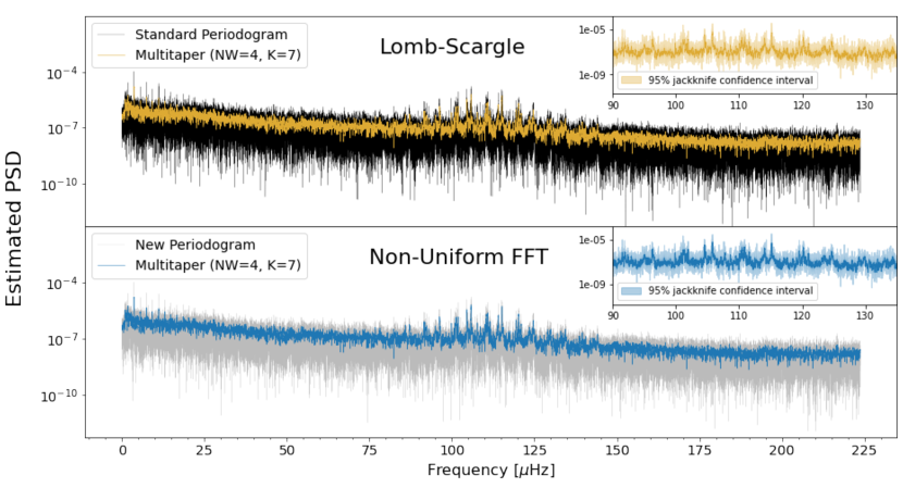
Figure 5: Comparison between the LS and the mtLS periodogram as well as that between the NUFFT and the mtNUFFT periodogram of the Kepler-91 time-series. The parameters of the multitaper periodograms are $NW=4$ and $K=7$. We clearly see that the multitaper periodograms in orange and pink have smaller variance as compared to their un-tapered counterparts in black and grey. The insets in the two panels show the zoomed-in mtLS and mtNUFFT periodograms respectively along with their 95% jackknife confidence intervals.

We can then compute the multitaper spectral estimate as follows

$$\hat{S}^{(\mathrm{mt})}(f)=\frac{1}{K}\sum_{k=0}^{K-1}\left|y_{k}(f)\right|^{2}$$ (10)

where $\left|y_{k}(f)\right|^{2}$ is the $k$th eigenspectrum $\hat{S}_{k}(f)$.

Instead of taking an average, we can weight each eigencoefficient $y_{k}(f)$ using an iterative adaptive weighting procedure (Thomson, 1982) to improve bias properties. Higher order tapers have lower bias protection and therefore are downweighted using adaptive weights $d_{k}(f)$ to obtain the spectral estimate

$$\hat{S}^{(\mathrm{mt})}(f)=\frac{\sum\limits_{k=0}^{K-1}\left|d_{k}(f)y_{k}(f)\right|^{2}}{\sum\limits_{k=0}^{K-1}\left|d_{k}(f)\right|^{2}}$$ (11)

where $d_{k}(f)$ are approximated as

$$d_{k}(f)=\frac{\sqrt{\lambda_{k}}S(f)}{\lambda_{k}S(f)+B_{k}(f)}$$ (12)

Here the spectrum $S(f)$ can be treated as signal and the broad-band bias $B_{k}(f)$ as noise. Since these two quantities are unknown, they are substituted by $\hat{S}(f)=\frac{1}{2}\left|y_{0}(f)\right|^{2}+\left|y_{1}(f)\right|^{2}$, the average of the $\hat{S}_{0}(f)$ and $\hat{S}_{1}(f)$ (lowest order) spectral estimates, and $\hat{B}_{k}(f)=(1-\lambda_{k})\sigma^{2}$, where $\sigma$ is the variance of the time-series $\bf{x}$. Then, Equations (11) and (12) are iteratively run, with $\hat{S}^{(\mathrm{mt})}(f)$ as the new $\hat{S}(f)$, until the difference between successive spectral estimates is less than a set threshold. The schematic diagram in Figure 4 illustrates the above described steps to compute multitaper spectral estimates.

We can also estimate confidence intervals on the multitaper spectral estimate by jackknifing over tapers (Thomson, 1991). Essentially, one computes delete-one spectral estimates $\hat{S}^{(\mathrm{mt})}_{\setminus j}(f)$ by omitting the $j$th eigencoefficient from Equation (10) or (11) to estimate a variance. The jackknife procedure provides a conservative variance estimate in practical scenarios where we cannot assume the data are Gaussian and stationary and/or rely on analytical distributions (e.g., $\chi^{2}$) to estimate errors. In addition to being distribution-free, it is an efficient estimator of variance as compared to the direct variance estimate obtained from individual eigenspectra $\hat{S}_{k}(f)$ (Thomson, 1991). We can see this efficiency in the case of Gaussian stationary data, where the jackknifed $\hat{S}^{(\mathrm{mt})}_{\setminus j}(f)$ have $\chi_{2K-2}^{2}$ distributions whose logarithms behave much better than those of $\hat{S}_{k}(f)$, which are $\chi_{2}^{2}$ distributed. Figure 7 demonstrates this behaviour of $\chi_{2}$ distributions, and Figure 5 shows jackknife confidence intervals for the multitaper spectral estimates described in Sections 2.2.3 and 2.2.4. We refer the reader to Thomson (1991) for more details.

2.2.3 Multitaper LS for Irregular Sampling

Springford et al. (2020) combine the Thomson multitaper statistic with the LS periodogram to compute the improved multitaper LS periodogram. Similar to the even sampling case, the mtLS tackles the problems of inconsistency and spectral leakage associated with the LS periodogram. The procedure to compute it for the series $\mathbf{x}=\{x_{n}\}$ corresponding to time stamps $\mathbf{t}=\{t_{n}\mid n=0,...,N-1\}$ is as follows:

1. Compute DPSS tapers $\mathbf{v}_{k}(N,W)$ of order $k=0,\dotsc,K-1$ at an even sampling grid with sampling interval $\overline{\Delta t}=T/N$ where $T=t_{n-1}-t_{0}$ using the tri-diagonal method,

2. Interpolate these tapers to the uneven sampling times $\mathbf{t}$ using a cubic spline and renormalize them to get $\mathbf{v}^{\star}_{k}(N,W)$, and

3. Compute $K$ independent LS periodograms $\hat{S}^{(\mathrm{LS})}_{k}(f)$ on the tapered time-series $v_{k,n}^{\star}x_{n}$. Their average represents the mtLS estimate $\hat{S}^{(\mathrm{mtLS})}(f)$.

It is important to note that the cubic spline interpolation of DPSS tapers maps the evenly-sampled tapers to irregular sampling but does not fully retain its optimal in-band concentration. The interpolation we discuss here is of the tapers only, not the time-series, to the irregularly spaced times $\mathbf{t}$. We show tapers interpolated to the Kepler-91 time stamps in Figure 4. Instead, the quadratic spectral estimator of Bronez (1988) uses generalized DPSS in the irregular sampling case to achieve minimal spectral leakage out of band. However, it comes at the expense of a computationally intensive matrix eigenvalue problem. In comparison, the mtLS statistic is fast to compute and a significant improvement over the LS periodogram, which is why we use it in this study.

Springford et al. (2020) apply this method to Kepler data to demonstrate how it improves upon the LS periodogram. We perform a similar analysis on the Kepler-91 time-series and show the results of comparison in Figure 5. The variance reduction of the mtLS periodogram is evident whereas its bias reduction is difficult to visualize even though we expect the spectral leakage properties to improve with multitapering. We therefore look at the mtLS pseudowindows and find that multitapering reduces bias and does not lead to the spurious peaks of the LS periodogram seen in Figure 3.

We extend the adaptive weighting and jackknife confidence intervals of the multitaper statistic for evenly-sampled time series (Thomson, 1982) to the mtLS. The top panel of Figure 5 shows the jackknife confidence interval of the mtLS periodogram of the Kepler-91 time-series.

2.2.4 Multitaper NUFFT for Quasi-Periodic Modes

In Section 2.1.2, we present the NUFFT periodogram that is ideal for detecting quasi-periodic modes as opposed to the purely periodic modes that the LS periodogram detects. We can combine this periodogram with the multitaper statistic to get the mtNUFFT periodogram. We use the same procedure as in Section 2.2.3 to compute this periodogram – the only modification is that in Step 3, we compute the eigencoefficients

$$y_{k}(f)=\sum_{n=0}^{N-1}v_{k,n}^{\star}x_{n}e^{-i2\pi ft_{n}},$$ (13)

using the (zero-padded) adjoint NUFFT to obtain the $\hat{S}^{(\mathrm{mt})}(f)$ through Equation (10). These eigencoefficients are the generalization of Equation (9) to the case of irregular sampling.

Figure 6: Both panels show the same pseudowindow as that in the bottom panel of Figure 3, but for the NUFFT and mtNUFFT periodograms. The top panel shows the spectral leakage properties of the mtNUFFT periodogram with $NW=1$ and $K=1$, i.e., the single-tapered spectral estimate, in blue, whereas the bottom panel shows the $NW=1.5$, $K=2$ mtNUFFT estimate in pink. It is clear that the mtNUFFT estimates have smaller spectral leakage than NUFFT. In the bottom panel, we observe that as $NW$ increases, the variance of the estimate reduces but the frequency resolution worsens.

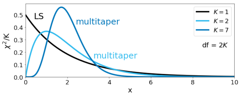
Figure 7: Comparison between distributions of LS and multitaper spectral estimates. LS is $\chi^{2}$ distributed with degrees of freedom $df=2$ as shown in black. mtLS and mtNUFFT are $\chi^{2}_{2K}$ distributed, where $K$ is the number of tapers. We show the $K=2$ ($\mathrm{df}=4$) and $K=7$ ($\mathrm{df}=14$) distributions in turquoise and blue curves. As $K$ (or df) increases, the $\chi^{2}_{2K}$ approaches a normal distribution with symmetric values around the mean, leading to better noise properties for the mtNUFFT periodogram.

The mtNUFFT estimation procedure is shown in Figure 4. In Figure 5, we compare the mtNUFFT periodogram with the NUFFT periodogram as well as with the LS and mtLS counterparts. All four spectral estimates are on the same frequency grid with an oversampling factor of 5. We see that the mtNUFFT periodogram behaves similar to the mtLS periodogram in the case of quasi-evenly-sampled time-series with gaps. We map adaptive weighting and jackknife confidence intervals to the mtNUFFT in the same way as the mtLS periodogram. Figure 5 shows the 95 % confidence interval of the mtNUFFT periodogram. In Figure 6, we use pseudowindows to show that any spurious peaks in the the NUFFT periodogram are removed by multitapering. We also observe that as the bandwidth $NW$ increases, the number of tapers one can use to generate the mtNUFFT periodogram increases ($K=2NW-1$) leading to an estimate with reduced variance, but the frequency resolution worsens due to increased local bias. We discuss this trade-off in the Appendix B and help the reader in choosing the parameters $NW$ and $K$.

In the following Section 2.3, we use a simulated asteroseismic time-series of a solar-like oscillator to illustrate that we can accurately model p-modes using mtNUFFT, significantly better than LS. We then validate these enhancements by applying mtNUFFT to the Kepler-91 light curve in Section 4. We discuss how this leads to precise age estimates for Galactic archaeology studies, and improved models of stellar structure and evolution.

Figure 8: Comparison between LS, mtNUFFT, and the true spectrum used to simulate an asteroseismic time-series (refer to Section 2.3 for more details of the simulation). The top and bottom panels show the $NW=3,\,K=5$ and $NW=4,\,K=7$ mtNUFFT periodograms respectively. The insets at the top right of the two panels zoom into two p-modes and show that mtNUFFT is able to estimate the PSD more accurately than the LS by reducing both bias and variance. We also see that the resolution slightly reduces as we increase $NW$, but it does not affect mode estimation in this case.

2.3 Simulated Time-Series of a Solar-like Oscillator

To illustrate the spectral estimation accuracy of the mtNUFFT periodogram, we simulate a light curve of a solar-like oscillator using an asteroseismic power spectrum model of a $1.0\;\mathrm{M}_{\odot}$ star of age $3.99$ Gyr and $Z=0.01$. We use a similar procedure as Ball et al. (2018) to simulate our synthetic power spectrum containing a granulation background and a p-mode envelope of a sum of Lorentzians

$$M(\bm{\theta},\nu)=b+\sum\limits_{n=1}^{N}\frac{h_{n}}{1+\frac{4}{w_{n}^{2}}(\nu-\nu_{n})^{2}}.$$ (14)

Here the parameters $\bm{\theta}$ are $T_{\mathrm{eff}},\Delta\nu,\nu_{\mathrm{max}},\epsilon$ (and more depending on the complexity of the model) which determine the background $b$, and heights $h_{n}$, widths $w_{n}$, frequencies $\nu_{n}$ of the Lorentzian profiles of the $N$ modes. $\bm{\theta}$ for a given stellar mass (and age) are easily computed using the scaling relations (Equations 25 and 26) and empirical data.

We refer to the $M(\bm{\theta},\nu)$ spectrum as the true PSD. We then use the algorithm in Timmer & Koenig (1995) to randomize the amplitude and phase of the Fourier transform corresponding to the true PSD that then generates a time-series through an inverse transform. Note that this algorithm generates an evenly-sampled time-series which we use as a simple case study for testing purposes. Similar arguments can be made for irregularly-sampled time-series, which we explore in Section 4.1 by analysing the Kepler-91 time-series.

After generating the synthetic light curve, we try to estimate the true PSD using the LS and mtNUFFT periodograms. We compute two mtNUFFT periodograms, one with bandwidth parameter $NW=3$ and another with $NW=4$. The number of tapers we use follow the $K=2NW-1$ rule. Figure 8 compares these mtNUFFT periodograms with LS. We observe the erratic behaviour and spectral leakage of the LS estimate (also shown in Figure 1 of Anderson et al. 1990), and the ability of the mtNUFFT periodogram to mitigate these problems. The noise in the LS estimate at any given frequency $\hat{S}^{(\mathrm{LS})}(f)$ is $\chi^{2}$ distributed with 2 degrees of freedom, whereas that in the mtNUFFT estimate $\hat{S}^{(\mathrm{mt})}(f)$ is $\chi^{2}_{2K}$ distributed. As $K$ increases, the $\chi^{2}_{2K}$ noise distribution approaches a (symmetric) normal, thereby improving upon the large noise values occurring in the $\chi^{2}_{2}\propto e^{-x/2}$ exponential tail. Figure 7 shows these properties of $\chi^{2}$ distributions. mtNUFFT also reduces out-of-band spectral leakage, and thus improves estimation of (central) frequencies, heights, and widths of the Lorentzians representing p-modes.

If you look closely at the inset in the bottom panel of Figure 8, you will notice the reduction of resolution and flattening of mode peaks with increasing bandwidth. However, the reduction does not affect mode estimation as the estimate has higher resolution than that required for studies of solar oscillations. Overall, this simple simulation study verifies that mtNUFFT can improve mode estimation.

Note that we do not show the low-frequency power excess in Figure 8 to focus on mode estimation, but do observe that the granulation background (or continuum) is better estimated using mtNUFFT. A good estimate of the continuum can help deduce granulation and rotational modulation properties (Kallinger et al., 2014), which when combined with mode estimates provide rigorous constraints on stellar models. These models can then inform the theory of stellar structure and evolution, and allow precise estimates of mass, radius, age, and other fundamental stellar properties.

In the following Section 3, we introduce the F-test as an extension of the mtNUFFT periodogram, and discuss how it makes this periodogram ideal for purely periodic signals, e.g. from exoplanet transits, in addition to the quasi-periodic p-modes we analyzed in this section.

3 Multitaper F-test for Exoplanet & stellar mode detection

In asteroseismology, we are often interested in determining whether a mode is strictly periodic or not because that informs us about the mode excitation mechanism. For e.g., p-modes are quasi-periodic in nature whereas g-modes and coherent quasi-infinite lifetime modes are closer to strictly periodic or sinusoidal shaped. In contrast, exoplanet transits embedded in asteroseismic time-series are observed as periodic oscillations with non-sinusoidal shapes. We illustrate these types of oscillations in Figure 9 and their corresponding frequency domain representations using the classical periodogram. Strictly or purely periodic signals are sinusoidal-shaped and are observed as line components in the Fourier domain, which are convolutions of delta functions with the rectangular window function of a time-series (refer to Figure 6 in VanderPlas 2018). The spectral representation of a quasi-periodic damped harmonic oscillation is a Lorentzian peak whose width depends on the damping rate. The periodic exoplanet transits with extremely non-sinusoidal shapes are decomposed into line components one at the fundamental frequency and the rest at harmonics. Thus, we can distinguish between different asteroseismic modes and exoplanet transits in the Fourier domain.

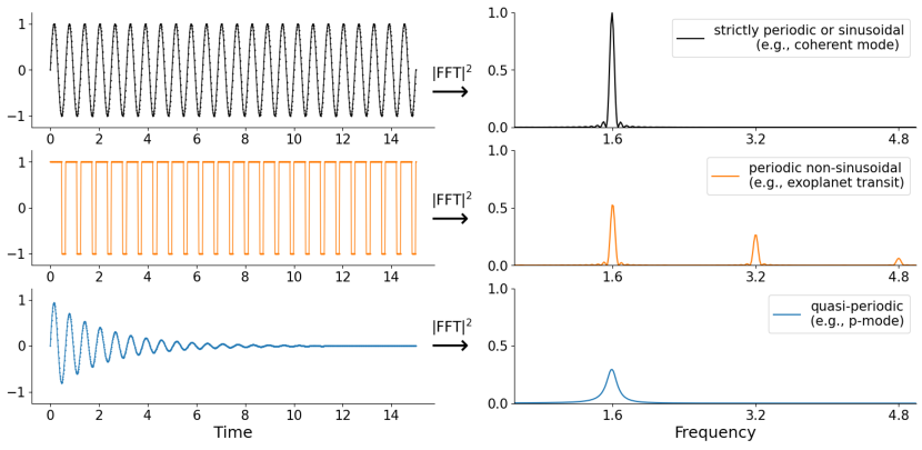
Figure 9: Comparison between strictly periodic or sinusoidal (top panel), non-sinusoidal-shaped periodic (middle panel), and quasi-periodic oscillations (bottom panel), which represent coherent modes, exoplanet transits, and p-modes respectively. The left panels show the oscillations in the time-domain using evenly-sampled time-series. The right panels show the corresponding spectral estimates by computing the classical periodogram. We see that in the Fourier domain, the strictly periodic or harmonic oscillation is seen as a peak at the frequency of the oscillation, the non-sinusoidal-shaped periodic oscillation is observed as line components representing the fundamental frequency and harmonics of the transit period, and the quasi-periodic or damped harmonic oscillations have Lorentzian frequency peaks with widths representing damping rates.

In the case of a solar-like oscillator, our aim is detect line components of exoplanet transits and Lorentzian profiles of p-modes on top of a continuous spectrum composed of stationary noise, granulation and/or magnetic backgrounds. We need harmonic analysis methods like the multitaper F-test (Thomson, 1982) to precisely detect the frequencies of line components embedded in such “mixed” spectra and estimate the periods of transitory exoplanets. We discuss this test in the next section.

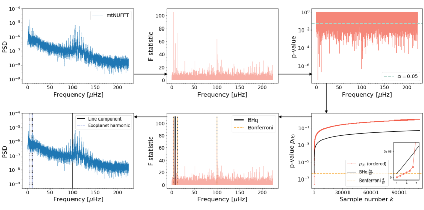
Figure 10: Schematic diagram showing the detection of purely periodic signals (line components) in the Kepler-91 time-series using multitaper F-test. First, we show the mtNUFFT periodogram with $NW=4$ and $K=7$ (top left) and its corresponding F statistic estimates (top middle). Then, we test the p-values of the F-test for significance (top right shows an example $\alpha=0.05$ level). Since we are testing multiple hypotheses, we perform selective inference by comparing the sorted p-values with the threshold curves of the Bonferroni and BHq procedures (bottom right). The inset in the bottom right panel zooms into the smallest p-values and shows that BHq rejects more hypotheses than Bonferroni. Finally, we plot the detected line components along with the F statistic estimates and the mtNUFFT periodogram (bottom middle and left). It is interesting to note that three BHq detected line components coincide with harmonic features that we expect to see due to the known transitory exoplanet Kepler-91b (Batalha et al., 2013; Lillo-Box et al., 2014).

3.1 F-test for Regular Time Sampling

Thomson (1982) develop the analysis-of-variance F-test for evenly-sampled time-series that estimates the significance of a periodic component embedded in coloured noise. It builds on top of the multitaper spectral estimate described in Section 2.2.2. Essentially, it computes a regression estimate of the power in the periodic signal of frequency $f$ using the eigencoefficients $y_{k}(f)$ of the time-series $\mathbf{x}$ and compares it with the background signal using the following $F$ variance-ratio

$$F(f)=\frac{(K-1)\left|\hat{\mu}(f)\right|^{2}\sum\limits_{k=0}^{K-1}\left|U_{k}(N,W;0)\right|^{2}}{\left|\sum\limits_{k=0}^{K-1}y_{k}(f)-\hat{\mu}(f)U_{k}(N,W;0)\right|^{2}}.$$ (15)

Here $U_{k}(N,W;0)$ is the DFT of the $k$th order DPSS taper $\mathbf{v}_{k}(N,W)$ at frequency $f=0$, and $\hat{\mu}(f)$ is the mean estimate of the amplitude of the periodic component at $f$ given by regression methods as

$$\hat{\mu}(f)=\frac{\sum\limits_{k=0}^{K-1}U_{k}(N,W;0)\,y_{k}(f)}{\sum\limits_{k=0}^{K-1}U_{k}(N,W;0)^{2}}.$$ (16)

The $F$ statistic in Equation (15) follows an F-distribution with $2$ and $2K-2$ degrees of freedom under the null hypothesis that there is no line component at frequency $f$, which we test for significance.

An important point to note here is that the F-test makes use of the phase information in the eigencoefficients $y_{k}(f)$, which are complex DFTs of DPSS tapered time-series data. Their phases help in the investigation of temporal variations and provide information that the power spectral density estimates fail to deliver. Particularly, the $y_{k}(f)$ have a complex Gaussian distribution under the F-test null hypothesis. Due to this extra information, F-test is extremely sensitive to (and preferentially picks) signals that resemble line components in the Fourier domain. In the context of asteroseismology, these purely periodic sinusoidal signals represent undamped modes or g-modes. On the other hand, the frequencies of damped quasi-periodic signals shift across a bandwidth surrounding a central frequency, e.g., a stochastically excited p-mode with intrinsic damping is described by a Lorentzian in frequency space.

3.2 F-test for Irregular Time Sampling

We extend the Thomson F-test to irregularly-sampled data using the eigencoefficients $y_{k}(f)$ computed for the mtNUFFT periodogram in Equation (13). Note that it is necessary to significantly zero pad the adjoint NUFFT that computes these $y_{k}(f)$ to ensure that the frequency grid spacing is small enough to detect all present line components. We thus zero pad to $M=5N$, similar to that in Figure 5.

Using the F-test along with the mtNUFFT periodogram opens avenues for accurately and precisely detecting different types of asteroseismic modes, backgrounds, and extrinsic features in photometric light curves. To demonstrate this, we apply our F-test to the Kepler-91 time-series and show the results in Figure 10, which we discuss in detail in the following Section 3.3.

3.3 Multiple testing problem

Each frequency in the multitaper spectral estimate has an associated F statistic, whose p-value determines the level of significance. If we test all these frequencies individually for significance, we run into the multiple testing problem. To understand this, consider the mtNUFFT periodogram in Figure 10 which has a total of 111,360 frequencies. For each frequency $f$, we either accept or reject the F-test null hypothesis by testing at the standard 5% significance level. Let us assume that there are 60 truly periodic signals amongst the 111,360 frequencies. Even in the best case scenario that our method detects all the 60 signals, it is also expected to flag 5% of the remaining 111,300 non-periodic signals as significant, i.e. $0.05*111,300=5565$ false positives (Janson et al., 2017).

To tackle this, we use selective inference, and control either the Familywise Error Rate (FWER) or the False Discovery Rate (FDR) for proper multi-hypothesis testing. These rates are defined as follows:

1. FWER is the probability of type I errors, i.e., the probability of having at least one false discovery.

2. FDR is the proportion of type I errors among discoveries.

The above definitions mean that FWER controlling procedures are generally more conservative than FDR. In Figure 10, we use both the Bonferroni and Benjamini Hochberg (BHq) procedures for controlling the FWER and FDR respectively at the 5% significance level ($\alpha=0.05$). The p-values are first sorted and then compared with the threshold curves of the two procedures. Bonferroni has a fixed threshold $\frac{\alpha}{M}$ whereas that of BHq is adaptive $\frac{k\alpha}{M}$, where $k$ is the sample number in the sorted list. We observe in the figure that BHq detects six hypotheses whereas Bonferroni detects three, and decide to choose the BHq discoveries for broader coverage of line components.

Our procedure detects four potential line components, which we follow-up to understand the nature of these signals. Note that we see four BHq lines instead of six due to splittings resulting from zero padding. The first three of these line components are at frequencies $0.320180$, $0.640186$, $0.960540$ cycles/day (${\approx}2/6.25,4/6.25,6/6.25$), which we expect to see due to the known transitory exoplanet, Kepler-91b, of period $6.246580\pm 0.000082$ days (Batalha et al., 2013). Thus, the F-test automatically detects the Kepler-91b transit harmonics, and provides period estimates of $6.246487,6.248179$ and $6.246486$ days from the three detected lines. In addition, we can estimate a variance (or uncertainty) of our frequency estimates by jackknifing over tapers (described in detail in the Section 3.4). For e.g., we obtain an estimate of $6.24648617\pm 0.002052$ days from the first line. Our uncertainty is only an order-of-magnitude higher than the most precise period estimates of the Kepler-91b exoplanet. These precise estimates are computed using specialized and computationally expensive methods, whereas the multitaper F-test is simple, efficient, and generally applicable.

The fourth detected line component seems to be situated near a $l=1$ mixed mode (Mosser et al., 2017). However, it is hard to determine if this is a genuine periodic signal linked to the mixed mode without further analysis. Fortunately, the variance of frequency estimates of line components (or the F-test statistic) is very efficient, and we leverage this property to follow-up our findings as follows.

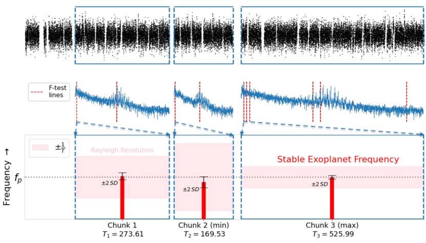
Figure 11: Schematic diagram demonstrating that the F-test frequency estimate $\hat{f}_{p}$ corresponding to the Kepler-91b transit harmonic $f_{p}=2/6.25$ is purely periodic. The top panel shows how we divide the Kepler-91 time-series into three chunks for studying the time evolution of $\hat{f}_{p}$. The middle panel shows the three corresponding mtNUFFT periodograms (blue), and their respective line detections using the BHq procedure with $\alpha=0.175$ for the F-test (red dashed lines). The bottom panel zooms into the $\hat{f}_{p}$ estimates of the three chunks (red bars) with frequency on the y-axis and chunk length ($T$) in days on the x-axis. The estimates are compared with $f_{p}$ using the two standard deviation jackknife uncertainties (black errorbars) and the Rayleigh resolution $1/T$ (pink) of the chunks. Both comparisons show that the estimates are consistent with $f_{p}$ and their uncertainties are a fraction of the Rayleigh resolution.

3.4 Variance of the F-test:
Investigating the nature of periodic signals

We demonstrate our follow-up approach by assuming an isolated periodic signal at frequency $f_{0}$ (separated from other lines by at least the bandwidth $W$). A good estimate of this frequency would be where the F-test is maximum

$$\hat{f_{0}}=\operatorname*{arg\,max}_{f}F(f)$$ (17)

In Figure 10, $\hat{f_{0}}$ corresponds to the Kepler-91b exoplanet transits. Under the assumptions of stationary Gaussian locally white noise and moderate SNR of the line $A\cos(2\pi f_{0}t+\phi)$ with constant amplitude $A$ and frequency $f_{0}$, the variance of the estimate $\hat{f_{0}}$ is given by

$$\mathrm{Var}\{\hat{f_{0}}\}=\frac{1}{\Xi_{K}}\frac{6}{{(2\pi T)}^{2}}\frac{S_{n}(f_{0})}{S_{l}(f_{0})}$$ (18)

where $\Xi_{K}$ is the variance efficiency in Thomson (1982) (refer to Appendix B for more details), $T$ is the total time duration of the observed series, $S_{n}(f_{0})$ is the noise (or background) spectrum at frequency $f_{0}$, and $S_{l}(f_{0})$ is the periodogram power spectral density of the line given by

$$S_{l}(f)=\frac{1}{4}A^{2}T$$ (19)

Equation (18) is the Cramér-Rao bound (e.g., Rife & Boorstyn, 1976) with an additional factor of ${\Xi_{K}}^{-1}$, i.e., it is a few percent larger than the bound (Thomson, 2007). Thus, for moderate ${\Xi_{K}}$ and $S_{l}(f_{0})/S_{n}(f_{0})$, the standard deviation of $\hat{f_{0}}$ is a fraction of $1/T$. This highlights an important property of the F-test estimator: it allows us to estimate line frequencies with uncertainties smaller than the Rayleigh resolution $1/T$.

In practice, we cannot directly use the analytical expression for variance because the (local) SNR $S_{l}(f_{0})/S_{n}(f_{0})$ is unknown, and the noise assumptions are rarely true. But one can estimate the variance by jackknifing over tapers as is done in Thomson (2007). There is empirical evidence that the F-test works well for lines isolated by one or two Rayleigh resolutions as opposed to the bandwidth $W$ (Thomson, 2007), and the jackknife uncertainties on frequency estimates are expected to be some fraction of Rayleigh resolution as in Equation (18).

We can further simplify Equation (18) by substituting Equation (19) in it. Doing so provides us the following relation:

$$\mathrm{Var}\{\hat{f_{0}}\}\propto\frac{1}{T^{3}}$$ (20)

which tells us that the variance of the F-test for lines is within a few percent of the Cramér-Rao bound, and so decreases like $1/T^{3}$. This proportionality demonstrates that reducing $T$ does not significantly increase the variance. Therefore, one can divide the time-series into shorter chunks and apply the F-test to detect line components across these chunks. Not only will this reduce the false detection probability (e.g., if you detect a line in two separate chunks at 99% significance, you reduce the probability to $10^{-4}$), but also help determine whether a signal is purely periodic, quasi-periodic with frequency shifts, or a false detection. Solar-like p-mode frequencies vary with activity, and hence will be rejected by the F-test for long time-series. Dividing time-series thus allows looking at the nature of stellar oscillations. We describe this as follows:

1. A purely periodic signal will be detected across all time chunks without any significant shifts (beyond estimate jackknife uncertainties) in its frequency estimates. We show this in Figure 11, which we discuss in detail later in this section.

2. Quasi-periodic p-modes with short lifetimes will undergo frequency shifts across consecutive chunks. They will also disappear and reappear in detections depending on their lifetimes. To distinguish between the shift of a mode frequency and neighbouring modes, we compare the frequency estimates to named modes and their widths in the literature. We illustrate this in Figure 12, which is also discussed later.

3. False signals will generally only appear in single isolated time chunks.

Another advantage of dividing time-series into chunks is that we can remove large gaps and analyze continuous quasi-evenly-sampled Kepler observations, thereby controlling spectral leakage and other issues associated with irregular sampling. As Kepler time-series are composed of ${\approx}3$ month quarters, using chunks of ${\sim}90$ days will ensure removal of large gaps. However, with $T=90$ days, the power spectral density of the line $S_{l}(f_{0})$ in question (refer to Equation 19) reduces significantly and detection becomes difficult. This is especially true for long periods (or low frequencies), as the variance of period estimates goes as

$$\mathrm{Var}\{\hat{P_{0}}\}=\frac{6P_{0}^{4}S_{n}(f_{0})}{\pi^{2}A^{2}T^{3}}$$ (21)

Therefore, to investigate the low-frequency $\hat{f_{0}}$ estimate in Figure 10, which corresponds to the Kepler-91b transit harmonic $f_{p}=2/6.25$ days, we remove large gaps and divide the Kepler-91 time-series into three chunks of lengths $T=273.61,169.53,525.99$ days. We show this in the top panel of Figure 11. Then, for each of the three chunks, we compute the mtNUFFT periodogram, apply the F-test to detect line components, and control the FDR using the BHq procedure with significance level $\alpha=0.175$, as described in Section 3.3. The middle panel of Figure 11 shows the three periodograms and their respective line detections. Note that we use a less conservative significance level for these detections compared to that for the entire time-series because the SNR of a line is proportional to $T$ (refer to Equation 19). We then focus on the detection $\hat{f}_{p}$ within the range $f_{p}\pm 2/T_{\mathrm{chunk}}$; we choose this range because the separability of lines for the F-test is on the order of one or two Rayleigh resolutions (as described earlier in this section). Finally, we estimate the variance of $\hat{f}_{p}$ by jackknifing over tapers. The $\hat{f}_{p}$ estimates for the three chunks and their two-standard deviation jackknife uncertainties (${\approx}95$% confidence interval) are in the bottom panel of Figure 11. This panel shows that the $\hat{f_{0}}$ estimate is very stable compared to the Rayleigh resolution as well as the jackknife uncertainties, which we expect from a purely periodic exoplanet signature. The jackknife uncertainties are ${\approx}1/6$ of the Rayleigh resolution, i.e., they are smaller for longer time chunks.

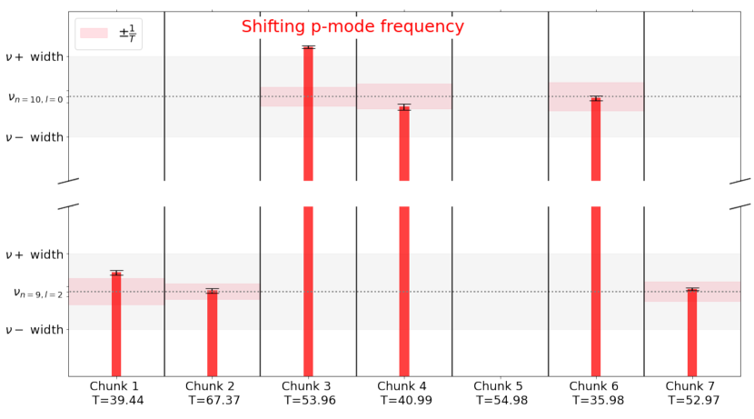
Figure 12: Detection of line components corresponding to two consecutive p-modes, $\nu_{n=9,\,l=2}=104.557\;\mu$Hz and $\nu_{n=10,\,l=0}=105.792\;\mu$Hz (Table 5 in Lillo-Box et al., 2014). The red bars indicate the $\hat{\nu}_{n,l}$ detections across seven time chunks, with roughly continuous and even sampling. The x-axis shows the lengths of these chunks ($T$) in days. The y-axis represents frequency, and helps compare the $\hat{\nu}_{n,l}$ estimates (red bars) and their jackknife uncertainties (black errorbars) with the mode frequencies $\nu_{n,l}$ and linewidths (Lillo-Box et al., 2014). The Rayleigh resolution of each chunk is also shown in pink. We see that $\nu_{n=9,\,l=2}$ is detected in chunks 1, 2, and 7, whereas $\nu_{n=10,\,l=0}$ is detected in chunks 3, 4, and 6. The frequency shifts and short-lived detections of modes is reminiscent of damped, short lifetime p-modes.

We then examine the behaviour of the high-frequency p-modes in Figure 10 by dividing the same time-series into seven chunks of length ${\sim}60$ days. Using the same method as in Figure 11, we compute the mtNUFFT periodograms and detect lines using the F statistic and multi-hypothesis testing. We then focus on two consecutive p-modes, $\nu_{n=9,l=2}=104.557\;\mu$Hz and $\nu_{n=10,l=0}=105.792\;\mu$Hz (Lillo-Box et al., 2014) by analyzing corresponding line detections. The correspondence is determined through comparison with the mode frequency and its linewidth. Across chunks, we see that the detected mode frequencies undergo shifts beyond jackknife uncertainties and the limiting Rayleigh resolution, thereby suggesting the presence of quasi-periodic p-modes. In some chunks, one of the modes is not detected at all, but it reappears at a later time; this property might have relations with the lifetime of p-modes. We can thus conclude that the F-test is a powerful tool to detect and characterize asteroseismic oscillations, thereby allowing determination of excitation mechanisms.

4 Age Estimation

In this paper, we have explored the advantages of multitaper spectral analysis for p-mode identification and characterization in red giants and other solar-like oscillators. A particularly interesting property of these solar-like modes is that they are (quasi-)evenly spaced in frequency, and their spacing has direct connections to fundamental stellar properties like mass, radius, and age. We can demonstrate these connections using the asymptotic theory of stellar oscillations as follows.

Assuming spherically symmetric stars, p-mode oscillations can be separated into radial and horizontal parts represented by radial order $n$ and spherical harmonic $Y_{l}^{m}$ with degree $l$ and azimuthal order $m$, respectively. $n$ is the total number of nodes along the radius, $l$ is the number of surface nodal lines, and $|m|\leq l$ is the number of nodal lines across the equator. We can approximate the frequencies of the high radial order modes ($l/n\to 0$) to first order (ignoring the $m$ wave number) as

$$\nu_{nl}\simeq\Delta\nu\left(n+\frac{l}{2}+\epsilon\right)$$ (22)

where $\epsilon$ is a phase term dependent on stellar boundary conditions and $\Delta\nu$ is the large frequency separation

$$\Delta\nu={\left(2\int_{0}^{R}\frac{dr}{c}\right)}^{-1}.$$ (23)

Here $c$ is the sound speed and $R$ is the stellar radius, which means that $\Delta\nu$ is the inverse of the travel time of a sound wave across the stellar diameter. Expanding Equation (22) to second order results in the small frequency separation $\delta\nu_{l\,l+2}(n)$ that breaks the degeneracy $\nu_{nl}\simeq\nu_{n-1\,l+2}$. We refer the reader to Aerts et al. (2010); Chaplin et al. (2011) for more details of the small frequency separation.

Due to its relations with the dynamical timescale of the star, it may be shown that $\Delta\nu$ is proportional to the square root of the mean density $\rho$ of the star.

$$\Delta\nu\propto\rho^{1/2}.$$ (24)

We can then obtain the following scaling relation (derivation in Kjeldsen & Bedding, 1995)

$$\frac{\Delta\nu}{\Delta\nu_{\odot}}\simeq\left(\frac{M}{M_{\odot}}\right)^{1/2}\left(\frac{R}{R_{\odot}}\right)^{-3/2}$$ (25)

which compares the $\Delta\nu$ of solar-like oscillations to that of the Sun.

Another global asteroseismic property is the frequency of maximum oscillation power $\nu_{\mathrm{max}}$ which is expected to be proportional to the acoustic cut-off frequency (Brown et al., 1991; Kjeldsen & Bedding, 1995; Belkacem et al., 2011). This proportionality forms the second scaling relation given as follows

$$\frac{\nu_{\mathrm{max}}}{\nu_{\mathrm{max,\odot}}}\simeq\left(\frac{M}{M_{\odot}}\right)\left(\frac{R}{R_{\odot}}\right)^{-2}\left(\frac{T_{\mathrm{eff}}}{T_{\mathrm{eff,\odot}}}\right)^{-1/2}$$ (26)

We can add observational constraints from non-seismic observations ($T_{\mathrm{eff}}$ estimates), and solve equations (25) and (26) to estimate stellar mass and radius as follows

$$\frac{M}{M_{\odot}}=\left(\frac{\nu_{\mathrm{max}}}{\nu_{\mathrm{max,\odot}}}\right)^{3}\left(\frac{\Delta\nu}{\Delta\nu_{\odot}}\right)^{-4}\left(\frac{T_{\mathrm{eff}}}{T_{\mathrm{eff,\odot}}}\right)^{3/2}$$ (27)

$$\frac{R}{R_{\odot}}=\left(\frac{\nu_{\mathrm{max}}}{\nu_{\mathrm{max,\odot}}}\right)\left(\frac{\Delta\nu}{\Delta\nu_{\odot}}\right)^{-2}\left(\frac{T_{\mathrm{eff}}}{T_{\mathrm{eff,\odot}}}\right)^{1/2}.$$ (28)

The mass relation then allows us to estimate precise stellar ages.

If we were to average the large frequency separation $\langle\Delta\nu\rangle$ between consecutive modes of the same degree $l$ in the power spectral estimate of a light curve, we would get a good estimate of $\Delta\nu$. However, $\langle\Delta\nu\rangle$ is sensitive to mode frequency estimates, and any noise or leakage in a power spectral estimate can lead to biased results. The same is true for $\nu_{\mathrm{max}}$ since it depends on the granulation background and power excess estimates. By reducing spectral leakage and noise (compared to LS), mtNUFFT improves p-mode characterization, and hence provides precise estimates of stellar mass, radius, and age through scaling relations. Beyond scaling relations, precise mode frequencies and damping rates as well as granulation and/or rotational modulation properties can provide fundamental constraints on stellar models.

In Section 4.1, we combine the mtNUFFT periodogram estimate of the Kepler-91 light curve with the PBjam Python package to perform peakbagging, i.e., estimate $\Delta\nu$, $\nu_{\mathrm{max}}$, and independent mode frequencies of the red giant. We show that these estimates are more precise than those from LS, and that this uncertainty improvement propagates to stellar mass, radius, and age estimation. We also demonstrate that peakbagging with mtNUFFT is more computationally efficient than LS, thereby allowing large scale asteroseismic analyses using PBjam.

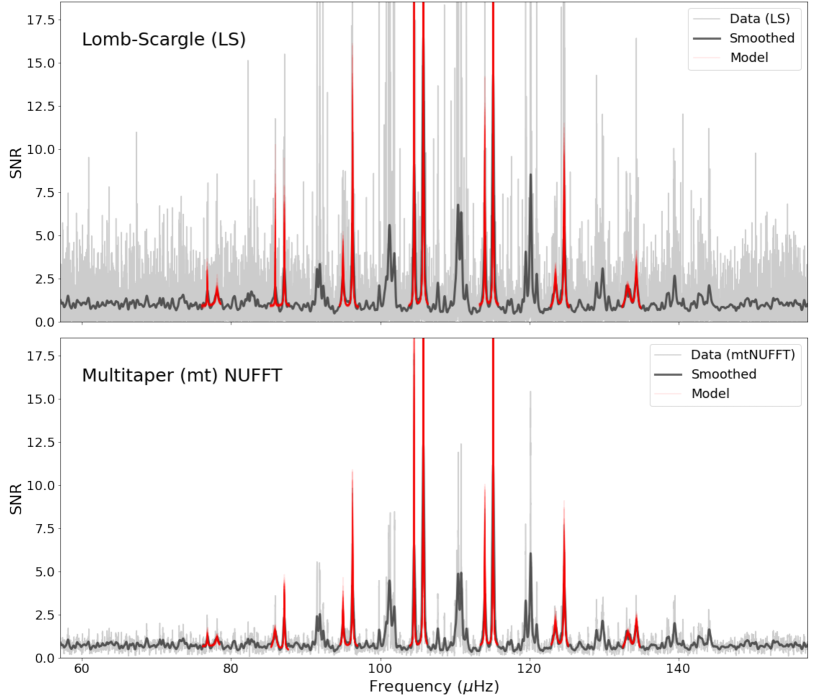
Figure 13: PBjam peakbagging fit for the Kepler-91 time-series using the LS (top panel) and mtNUFFT (bottom panel) periodograms. Both panels show a SNR spectral estimate (data) in grey along with its smoothed version using a 1D Gaussian filter kernel in black. The panels also show the model fits (red) to the radial $l=0$ and quadrupole $l=2$ modes obtained in Step 3 of PBjam. It is evident that the variance of the mtNUFFT SNR spectral estimate is much smaller than that of the LS periodogram, which leads to more efficient peakbagging than LS.

4.1 Kepler-91 Red Giant Time-Series

We now compare spectrum estimation using the LS and mtNUFFT periodograms by applying them to a Kepler light curve of a solar-like oscillator. We use the same Kepler-91 red giant case study we have been using throughout this paper. For the comparison, we use the following procedure:

1. Compute the LS and mtNUFFT periodograms of the time-series

2. Analyze the two spectral estimates using the PBjam (Nielsen et al., 2021) package that measures the frequencies of the radial ($l=0$) and quadropole ($l=2$) oscillation modes of the red giant to infer fundamental stellar properties like mass, radius, and age

3. Compare the efficiency and accuracy of stellar property inference in step (2) for the two spectral estimates

The above procedure directly applies PBjam to both the LS and mtNUFFT spectral estimates. While this seems straightforward, there are several statistical assumptions involved that we need to address. We can understand these assumptions by examining the steps involved in PBjam analysis. At its core, PBjam uses a Bayesian approach to fit a solar-like asteroseismic model to the power spectral estimate of a light curve. It obtains the posterior distribution given the likelihood and the prior distribution

$$P(\bm{\theta}|D)=P(D|\bm{\theta})*P(\bm{\theta})$$ (29)

where $\bm{\theta}$ represents the set of parameters of a solar-like power spectrum model, e.g., Equation (14), $D$ is the data that includes the SNR spectral estimate. The lightkurve package (Lightkurve Collaboration et al., 2018) generates this SNR estimate by dividing the periodogram power by an estimate of the background (a flattened periodogram). For more details on the preprocessing, refer to Lightkurve Collaboration et al. (2018). PBjam automates this procedure in three major steps:

1. KDE: This step first computes a kernel density estimate (KDE) of the prior $P(\bm{\theta})$ using previously fit $\bm{\theta}$ of 13,288 Kepler stars. Then, it uses the KDE prior and the inputs to PBjam to estimate a starting point for next step. The inputs are $T_{\mathrm{eff}}=4643.4\pm 67.3$ (APOKASC-2; Pinsonneault et al., 2018), $\Delta\nu=9.48\pm 0.88\,\mu\mathrm{Hz}$, and $\nu_{\mathrm{max}}=109.4\pm 6.1\,\mu\mathrm{Hz}$ (calculated using the A2Z pipeline of Mathur et al. 2010 in Lillo-Box et al., 2014). This step remains the same for both mtNUFFT and the standard LS spectral estimates.

2. Asy_peakbag: Given the prior $P(\bm{\theta})$ and starting point from the previous step, Asy_peakbag performs a fit to the asymptotic relation of radial and quadrupole modes (refer to Equations 22 and 14) by estimating the posterior probability as

   $$\ln P(\bm{\theta}|D)=\ln\mathcal{L}(\bm{\theta})+\ln P(\bm{\theta})$$ (30)

   where the log-likelihood is given by

   $$\ln\mathcal{L}(\bm{\theta})=\ln\mathcal{L}_{\hat{S}}(\bm{\theta})+\ln\mathcal{L}_{O}(\bm{\theta})$$ (31)

   Here $\ln\mathcal{L}_{\hat{S}}(\bm{\theta})$ is the likelihood of model $M(\bm{\theta},\nu)$ given SNR spectral estimate $\hat{S}_{j}$ at $j=\{1,\dotsc,J\}$ frequency bins (refer to Nielsen et al. 2021 for information on $\mathcal{L}_{O}$). For LS spectral estimates $\hat{S}^{(\mathrm{LS})}$ that are $\chi^{2}_{2}$ distributed about the expectation $M(\bm{\theta},\nu)$, the likelihood is (Woodard, 1984; Duvall & Harvey, 1986; Anderson et al., 1990)

   $$\ln\mathcal{L}_{\hat{S}^{(\mathrm{LS})}}(\bm{\theta})=-\sum\limits_{j=1}^{J}\left(\ln M(\bm{\theta},\nu_{j})+\frac{\hat{S}^{(\mathrm{LS})}_{j}}{M(\bm{\theta},\nu_{j})}\right)$$ (32)

   This likelihood does not directly apply to mtNUFFT estimates $\hat{S}^{(\mathrm{mt})}$ as they are $\chi^{2}_{2K}$ distributed about $M(\bm{\theta},\nu)$ (refer to Section 2.3). However, Anderson et al. (1990) show that the likelihood of a $\chi^{2}_{2K}$ distributed spectral estimate is

   $$\ln\mathcal{L}_{\hat{S}^{(\mathrm{mt})}}(\bm{\theta})=K\ln\mathcal{L}_{\hat{S}^{(\mathrm{LS})}}(\bm{\theta})$$ (33)

   which means that we can still maximize $\ln\mathcal{L}_{\hat{S}^{(\mathrm{LS})}}(\bm{\theta})$ for fitting $M(\bm{\theta},\nu_{j})$ to mtNUFFT estimates. The only difference is that the uncertainties (or errors) on $\hat{\bm{\theta}}$ reduce to

   $$\delta\hat{\bm{\theta}}^{(\mathrm{mt})}=\frac{\delta\hat{\bm{\theta}}^{(\mathrm{LS})}}{\sqrt{K}}.$$ (34)

   Thus, this step in PBjam does not change for mtNUFFT, but the errors get divided by $\sqrt{K}$.

3. Peakbag: This final step fits a more relaxed model to the spectral estimate than the asymptotic relation in Step 34. The solar-like spectrum model $M(\bm{\theta},\nu)$ in Equation (32) is refined to $M_{n}(\nu)$ for each pair of modes ($n,l=0$) and ($n-1,l=2$), and $\hat{S}^{(\mathrm{LS})}$ is over frequency bins that span the mode pair. The likelihood of the refined model given the $\chi^{2}_{2}$ distributed LS estimate stays the same as in Equation (32). Thus, this step does not change for mtNUFFT with the exception of reduced uncertainties as in Equation (34).

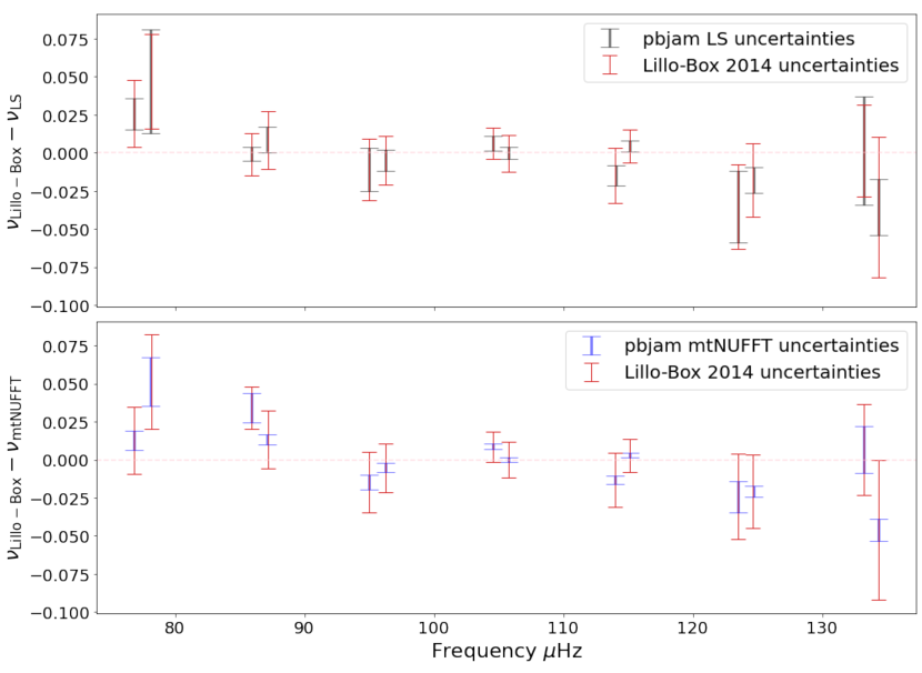
Figure 14: Comparison between mode frequency estimates $\nu_{\mathrm{Lillo-Box}}$ (Lillo-Box et al., 2014), $\nu_{\mathrm{LS}}$ (PBjam + LS) and $\nu_{\mathrm{mtNUFFT}}$ (PBjam + mtNUFFT). The x-axis of the red errorbars represents $\nu_{\mathrm{Lillo-Box}}$ for $l=0,2$ modes, whereas those in grey (top panel) and blue (bottom panel) show the PBjam $\nu_{\mathrm{LS}}$ and $\nu_{\mathrm{mtNUFFT}}$ respectively. The y-axis plots the difference between the published and PBjam estimates: $\nu_{\mathrm{Lillo-Box}}-\nu_{\mathrm{LS}}$ in the top panel and $\nu_{\mathrm{Lillo-Box}}-\nu_{\mathrm{mtNUFFT}}$ in the bottom panel. The errorbars show the $1\sigma$ uncertainties (or 68% confidence intervals) on the frequency estimates. We observe that the three sets of estimates are consistent, but $\nu_{\mathrm{mtNUFFT}}$ is much more precise than $\nu_{\mathrm{LS}}$ and $\nu_{\mathrm{Lillo-Box}}$.

Anderson et al. (1990) deal with the problem of estimating the Lorentzian profile of a mode with a given degree $l$ by averaging over $m$ mode splittings. This “m-averaging” procedure is statistically similar to averaging eigencoefficients for obtaining mtNUFFT estimates. Therefore, their problem directly translates to ours, allowing us to directly apply PBjam to both the LS and mtNUFFT periodograms. The only change is the division of estimate uncertainties by $\sqrt{K}$. Thus, mtNUFFT provides more precise estimates than LS.

Table 2: Inference of average seismic and stellar parameters

	$\Delta\nu$ ($\mu$Hz)		$\nu_{\mathrm{max}}$ ($\mu$Hz)		Mass ($\mathrm{M}_{\odot}$)		Radius ($\mathrm{R}_{\odot}$)		Log Age ($\mathrm{Myr}$)		% Age Uncertainty
	Mean	Std	Mean	Std	Mean	Std	Mean	Std	Mean	Std
mtNUFFT	9.4308	0.0014	110.0476	0.1335	1.3728	0.0303	6.5551	0.0482	3.5978	0.0495	12.0713
LS	9.4289	0.0039	109.8901	0.3721	1.3680	0.0330	6.5483	0.0528	3.6030	0.0514	12.5711
(cor) APOKASC-2	9.4370	0.0378	109.4450	0.9850	1.2190	0.0463	6.1810	0.0865	3.8320	0.0610	15.0800
(uncor) APOKASC-2					1.3473	0.0513	6.5109	0.0910	3.6299	0.0702	17.5308

Note. — Comparison between PBjam mean and standard deviation estimates of average seismic and stellar parameters using LS and mtNUFFT periodograms. These estimates are also compared with the APOKASC-2 uncorrected and corrected scaling relation estimates.

We now compare PBjam asteroseismic inference of the Kepler-91 light curve using LS and mtNUFFT periodograms. Figure 13 shows the peakbagging fit for both the periodograms. We immediately notice that since the variance of the mtNUFFT SNR spectral estimate is small, smoothing it using a 1D Gaussian filter kernel with standard deviation $\sigma=1/\Delta f$ results in a similar estimate. This is not the case for LS, where smoothing using the same Gaussian filter kernel results in a significant variance reduction. Thus, it is computationally efficient to perform peakbagging with mtNUFFT rather than LS. We compare the wall-clock time taken by the final peakbagging step 3 for the two periodograms, and find that mtNUFFT provides a factor three speed-up.

Note that smoothing or averaging the LS periodogram to compute a spectral estimate with reduced variance is not the same as computing a multitaper spectral estimate. This is because the smoothed LS estimate averages over signal and leakage leading to false mode detections and inaccurate frequency estimates. Thus, in addition to efficiency, we test the accuracy and precision of estimation. The top panel of Figure 14 compares the PBjam $l=0,2$ mode frequency estimates using LS and mtNUFFT with published estimates in Lillo-Box et al. (2014). We see that the two sets of PBjam estimates are consistent with the literature values, and that the $1\sigma$ uncertainties on the mtNUFFT estimates, especially for high SNR mode estimates, are much smaller than LS. We also see that there are small differences between the LS and mtNUFFT (mean) mode estimates, which could be because of reduction in spectral leakage and variance (noise) provided by mtNUFFT.

Along with frequency, PBjam infers mode widths and heights. We improve the precision of such (line)width estimates by using mtNUFFT. These estimates can help derive the lifetimes and damping rates of p-modes that are challenging to estimate in red giants (Hekker & Christensen-Dalsgaard, 2017). This problem is harder when dealing with mixed modes (e.g., $l=1$), which are not considered in PBjam due to their complex spectral structures. We discuss the prospects of mtNUFFT for mixed modes in Section 5.

In Table 2, we compare the estimates of average seismic parameters, $\Delta\nu$ and $\nu_{\mathrm{max}}$, using PBjam with LS and mtNUFFT periodograms. We see that the two sets of mean estimates are consistent, even more than the individual mode frequency estimates. The smaller differences are because these properties are estimated by averaging over several modes. Thus, the inferred estimates of bulk stellar properties like mass and radius are similar for mtNUFFT and LS when using scaling relations. Note that both our PBjam estimates are also consistent with those from the APOKASC-2 sample (Pinsonneault et al., 2018) that combines Kepler asteroseismic time-series with the APOGEE spectroscopic sample.

The standard deviations on the PBjam estimates are much smaller than the uncertainties on the APOKASC-2 estimates (refer to Table 2), thereby illustrating that PBjam peakbagging provides precise estimates. In addition, the standard deviations on the mtNUFFT estimates are much smaller than LS, allowing more precise estimates of bulk stellar properties. Particularly, the mtNUFFT uncertainties on $\Delta\nu$ and $\nu_{\mathrm{max}}$ are ${\approx}0.36$ (or ${\approx}1/\sqrt{K}$) times the respective LS uncertainties, leading to reduction of stellar mass and radius uncertainties to ${\approx}0.91$ times the LS uncertainties. We see that the mass and radius uncertainty reduction is smaller compared to that of $\Delta\nu$ and $\nu_{\mathrm{max}}$. We can understand this by propagating $\Delta\nu$ and $\nu_{\mathrm{max}}$ uncertainties into the mass and radius scaling relations (27) and (28). The following mass uncertainty formula is derived using error propagation through partial derivatives with the assumption that the uncertainties on $\Delta\nu$, $\nu_{\mathrm{max}}$ and $T_{\mathrm{eff}}$ are small

$$\sigma_{M/M_{\odot}}^{2}=\left(\frac{M}{M_{\odot}}\right)^{2} \left[9\left(\frac{\sigma_{\nu_{\mathrm{max}}}}{\nu_{\mathrm{max}}}\right)^{2}+16\left(\frac{\sigma_{\Delta\nu}}{\Delta\nu}\right)^{2}\right.$$

$$\left.+2.25\left(\frac{\sigma_{T_{\mathrm{eff}}}}{T_{\mathrm{eff}}}^{2}\right)\right].$$ (35)

Thus, the uncertainty on stellar mass is dominated by the fractional uncertainties of $\Delta\nu$ and $\nu_{\mathrm{max}}$ with factors 16 and 9 respectively in Equation (35). However, for our case study of Kepler-91, these uncertainties are very small, on the order of $0.01$ and $0.1$% respectively (refer to columns mtNUFFT and LS in Table 2). In contrast, the $T_{\mathrm{eff}}$ fractional uncertainty is ${\approx}1.45\%$, which contributes more to the total mass error despite its $2.25$ factor in Equation (35). The same is true for stellar radius uncertainty. Instead of directly using the formula in Equation (35) to list mass uncertainties in Table 2, we estimate these uncertainties by drawing $\Delta\nu$, $\nu_{\mathrm{max}}$, and $T_{\mathrm{eff}}$ samples from normal distributions with means and standard deviations given in Table 2 (and $T_{\mathrm{eff}}=4643.4\pm 67.3$ in APOKASC-2) and applying uncorrected scaling relations. We then confirm that these uncertainties is consistent with Equation (35). We repeat this procedure for stellar radius estimates.

Finally, we propagate the stellar mass uncertainty to age. We use the scipy piecewise linear interpolation on the APOKASC-2 sample to estimate their mapping from (mass, $[\mathrm{Fe/H}])\rightarrow$ age. This empirically approximates the stellar age function $f(\mathrm{mass},[\mathrm{Fe/H}]))$ using the stellar models computed by APOKASC-2. We then compute the implied age of Kepler-91 using our mass estimates and $[\mathrm{Fe/H}]$ estimates from APOKASC-2. The uncertainties are computed in the same way we compute age and radius uncertainties, i.e., by sampling normal distributions with means and standard deviations given by corresponding estimates of mass and $[\mathrm{Fe/H}]$. We compare our PBjam age estimates with the APOKASC-2 age estimates using uncorrected scaling relations and those with corrections applied (refer to Pinsonneault et al. 2018 for more details). We find that age uncertainties using PBjam are much more precise than those from APOKASC-2. In addition, we find that using mtNUFFT with PBjam instead of LS reduces age uncertainties from $12.6$ to $12.1$%. Thus, we expect that we improve age uncertainties for other solar-like oscillators, especially those with low SNR light curves since their $\Delta\nu$ and $\nu_{\mathrm{max}}$ fractional uncertainties will be larger. We could also aim to achieve $\lesssim 10$% precision in age by targeting the high SNR light curves.

Note that the uncorrected scaling relations (27) and (28) assume that we can scale all solar-like oscillators to the Sun, an approximation that does not entirely hold for the evolved stars. For example, the $l=1$ modes in red giants have mixed p and g-mode characteristics. These mixed mode frequencies and widths are hard to estimate and are thus not yet included in PBjam. We expect that mtNUFFT will provide more accurate stellar property estimates if stellar models are constrained using independent frequency estimates, including the $l=1$ modes. Thus, PBjam should be extended to these modes and corrections to scaling relations should be made based on stellar modeling.

5 Discussion

In this section, we discuss the advantages of our statistical methods and their prospects for asteroseismology, with a particular focus on stellar structure and evolution as well as Galactic archaeology studies. We also mention their limitations and highlight potential improvements.

5.1 Prospects for Asteroseismology

In the case of solar-like oscillators, multitaper spectral analysis allows precise estimation of the frequencies, widths, and heights of the Lorentzians that represent p-modes. This improvement can help us go beyond scaling relations and test detailed models of stellar structure and evolution. In addition, it provides more precise age estimates of solar-type and red-giant stars than the state-of-the-art, which has promising implications for Galactic Archaeology (Chaplin & Miglio, 2013).

In a forthcoming paper, we will extend mtNUFFT to red giants in old open clusters. Stars in open clusters are believed to form in well-mixed giant molecular clouds (Shu et al., 1987; Lada & Lada, 2003), and therefore have similar ages and chemical abundances. We will use these clusters to investigate the overall improvement in stellar mass, radius, and age precision provided by our method. In addition, mass estimation of red giants in open clusters allows the measurement of the mass loss along the red giant branch (RGB). Understanding RGB mass-loss is crucial for constraining models of stellar evolution; it dictates the temperature on the Horizontal Branch and the subsequent evolution on the AGB. It also plays an important role in the chemical enrichment of galaxies (Handberg et al., 2017). We will thus build upon the work of Miglio et al. (2012) and apply mtNUFFT to precisely estimate RGB mass loss using open clusters.

We then plan to apply our method to a large number of field stars in the Kepler field. To better understand the role of spectral leakage in Kepler data, we will look at stellar candidates whose LS and mtNUFFT estimates have large differences. Following this study, we will combine our precise stellar age estimates with abundances to empirically estimate the age-metallicity relation of the Milky Way disk.

In Section 4.1, we only dealt with radial and quadrupole modes in the red giant Kepler-91. The $l=1$ mixed modes are coupled to gravity waves in the stellar core, leading to deviations from the regular spacing pattern defined by $\langle\Delta\nu\rangle$ pattern. If we were to improve the precision of the $l=1$ mode width estimates using mtNUFFT, we would be able to derive damping rates and mode lifetimes of mixed modes that probe the stellar cores and the core-envelope boundary conditions, particularly the mass, size, rotation, and evolutionary state (Bedding et al., 2011) of the helium core. Frequency analysis of red giant $l=1$ modes with mtNUFFT could also help diagnose the nature of depressed dipole modes and determine if they are indeed mixed modes (Mosser et al., 2017).

mtNUFFT can further constrain the low-frequency power excess that can help deduce stellar granulation (surface convection), rotational modulation, and other stellar activity (refer to García & Ballot, 2019, for a review). Empirical evidence suggests that the properties of these granulation background signals (characteristic timescale and brightness fluctuation) scale with $\nu_{\mathrm{max}}$. Kallinger et al. (2014) compare different models for granulation backgrounds and show that a two-component super-Lorentzian function generally works well for Kepler solar-like oscillators. However, the uncertainty in the model choice introduces systematic errors in $\nu_{\mathrm{max}}$ estimates, which we can control through precise modeling using mtNUFFT. Also note that Kallinger et al. (2014) perform gap filling using interpolation to reduce leakage of the low-frequency granulation signal to high frequencies, but this method itself can lead to some spectral leakage and bias in spectral estimates (Lepage & Thomson, 2009; Springford et al., 2020). We can instead use mtNUFFT to control spectral leakage and better estimate granulation backgrounds. mtNUFFT can also be combined with the multitaper F-test to estimate rotation peaks and harmonics.

In addition to solar-like oscillators, we can use multitapering to analyze different classes of pulsating stars that span the Hertzsprung-Russell diagram (Aerts, 2021). Precise estimation of mode frequencies and lifetimes, whether they are p, g, or heat-driven undamped modes, opens avenues for detailed studies of stellar interiors. We believe that the mtNUFFT combined with the F-test would be an improvement over the iterative prewhitening (Breger et al., 1993) method, which couples frequency extraction in the Fourier domain with least-squares fitting in the time-domain to search for g or undamped modes with long lifetimes in different pulsators (e.g., the period spacing pattern estimation of $\gamma$ Doradus stars in Van Reeth et al., 2015a, b; Li et al., 2020; Aerts, 2021). We explore the detection of g-modes in slowly-pulsating B stars using the multitaper F-test in a forthcoming paper.

An important point to note is that our method has great potential for analyzing ground-based asteroseismic time-series from single or multiple sites. These time-series are strongly gapped and suffer immensely from leakage, especially when combined with a prewhitening process. We believe that our method could provide a larger improvement over LS for these data as compared to Kepler and other space-based photometry.

5.2 Statistical Advantages and Improvements

The LS periodogram is a widely-used spectral estimate for unevenly-sampled time-series analysis, particularly in asteroseismology. Scargle (1982) designed this periodogram for the detection of a single strictly periodic (sinusoidal) signal hidden in white noise. For other types and combinations of signals and/or noise, spectral leakage and variance of the periodogram is a problem. Springford et al. (2020) resolve this by combining the multitaper spectral estimator (Thomson, 1982) with the LS periodogram. We take a step further, and combine multitapering with the NUFFT periodogram to improve upon the periodicity conditions of the LS periodogram. Figures 5 and 6 demonstrate the spectral leakage and variance reduction of the mtLS and the mtNUFFT periodograms, and show that their noise properties have significant improvements compared to the LS (also seen in Figure 7). The figures also report the jackknife uncertainties on the spectral estimates, which provide realistic confidence intervals compared to the theoretical $\chi^{2}$ error distributions that depend on simplifying assumptions.

We also develop the multitaper F-test (Thomson, 1982) for the mtNUFFT periodogram, one of the first extensions of the Thomson F-test to uneven sampling. Figures 10, 11, and 12 illustrate how powerful the F-test is for diagnosing the nature of periodic signals over time. This has promising implications for asteroseismology (as discussed in Section 5.1) as well as for time-domain astronomy in general (for e.g., Huppenkothen et al., 2013).

There are several ways in which we could refine the mtNUFFT periodogram. The spline interpolation in Springford et al. (2020) could be improved for accuracy, while still maintaining its computational gain over the generalized DPSS for irregular sampling (Bronez, 1988). Chave (2019) revisit the methodology in Bronez (1988) and compute a mutlitaper estimator for time-series data with gaps. The missing data problem is solved efficiently without interpolation and improves upon previously developed approaches (Fodor & Stark, 2000; Smith-Boughner & Constable, 2012). However, the limitation of this method is that it runs into issues when dealing with truly irregular samples and several short duration gaps. We aim to compare this method with our approach, and see how much the quasi-regularity and gaps in the time-series affect the results.

In Appendix B, we discuss how the optimization of the bandwidth $NW$ and the number of tapers $K$ is an open problem, but several strategies can be used to estimate them. Using the example of a damped oscillator (Lorentzian), Haley & Anitescu (2017) optimize $NW$ for smooth spectra. We can extend this simple example to a series of Lorentzians on top of a low-frequency power excess or red noise, but work needs to be done to handle (or remove) line components using the F-test and its variance ($\hat{f}_{0}$ uncertainties). $K$ is usually set to $2NW-1$ to control out-of-band spectral leakage, but this discrete parameter could be tuned to ensure minimal spectral leakage.

Time-series analysis, and particularly spectral analysis, methods are generally well established for stationary processes, and multitaper spectral analysis is no exception. Stationarity assumes that the statistics underlying a process are constant, that is, the joint probability distribution (strongly stationary) or the mean and covariance (weakly stationary) do not evolve over time. However, real data is often not strictly stationary (Thomson, 1982; Nason, 2006), and this is true for several astrophysical processes. We could in principle search for non-stationarities in asteroseismic data using the multitaper test in Marshall et al. (2018). Note that spectral analysis is reasonably robust to non-stationarities, i.e., it can detect a periodic signal with time-varying amplitude and frequency, but its accuracy can be improved by explicitly taking stationarity and non-linearity into account (Rahim et al., 2014a). Therefore, multitaper spectral analysis has been extended to include non-stationary processes, e.g. the Loève spectrum in Thomson (1982) and the widely-used overlapping sliding window method (Hammond & White, 1996). In the future, these could be extended to unevenly-spaced asteroseismic data.

We explored the advantages of multitapering for analyzing Kepler data. These advantages are also applicable to other space-based and potentially ground-based missions, but care needs to be taken to handle different baselines and sampling times. For example, the NASA-Transiting Exoplanet Survey Satellite (TESS) mission (Ricker et al., 2014) provides high-precision photometric time-series of stars for a field of view $\sim$400 times larger than that of Kepler with baselines between 27 and 351 days and cadence of 30, 10, 2 minutes, and 20 seconds. Thus, the TESS mission has shorter baselines, particularly for observations not in the continuous viewing zones, making the Rayleigh resolution and frequency precision lower. For this case, smaller $NW$ would generally work well. On the other hand, ground-based observations have larger gaps and more uneven sampling, and thus improvements over the NUFFT algorithm might be necessary. Most NUFFT algorithms internally compute an FFT over a fine grid of evenly sampled times that is interpolated to uneven time stamps using certain kernels (e.g., FINUFFT; Barnett et al., 2019). Largely uneven sampling times could thus affect the performance of these NUFFT algorithms.

6 Conclusion

In this paper, we introduce mtNUFFT that combines the generalized periodogram with multi-tapering to accurately estimate the power spectrum underlying an irregularly-sampled time-series. The generalized periodogram is an extension of the classical periodogram (Schuster, 1898) to irregular sampling using a non-uniform FFT that is designed to detect and characterize non-sinusoidal periodic and quasi-periodic signals better than the LS periodogram. Multi-tapering (Thomson, 1982) refers to windowing of time-series using DPSS tapers that minimize bias (spectral leakage) and variance (noise) of the periodogram estimate. mtNUFFT particularly works well for quasi-regular time sampling with gaps such as that of space-based Kepler light curves.

Using simulations and the case study of the Kepler-91 red giant light curve, we show that mtNUFFT provides accurate and precise spectral estimates of solar-like oscillators. We are able to characterize quasi-periodic p-modes better than LS, and push the boundaries of stellar age precision achieved beyond the state-of-the-art. For Kepler-91 in particular, we obtain an age estimate of $3.96\pm 0.48$ Gyr with $36$% better precision than the APOKASC-2 (uncorrected) estimate of $4.27\pm 0.75$ Gyr.

We also demonstrate that our multitaper method can test the presence of line components in a spectrum using the F-statistic. Line components in an asteroseismic time-series could be due to exoplanet transits or stellar activity such as rotational modulation and coherent modes. Using this multitaper F-test alone, we detect and estimate the period of the Kepler-91b exoplanet, $6.246\pm 0.002$ days, with only an order-of-magnitude higher uncertainty than the most precise estimates. The variance of the F-test allows us to diagnose the periodicity or quasi-periodicity of different signals. For example, we can divide a Kepler time-series into shorter, more continuous chunks and test whether the frequency of a signal remains stable over the duration of the light curve. This technique has prospects for determining excitation mechanisms of asteroseismic modes, thereby providing deeper insights into stellar structure and evolution.

Our method also extends to ground-based asteroseismic time-series with potentially larger improvements over LS because these data greatly suffer from leakage. The application of our method to space and ground-based asteroseismic time-series has prospects for the following astronomical studies

1. Stellar structure and evolution:

   1. Low-mass stars: p & mixed modes

   2. Intermediate/high-mass: g & coherent modes

   We aim to extend our mtNUFFT results on p-mode characterization and frequency shifts to a sample of stars and compare with literature values. Our current focus is on red giants and slowly-pulsating B stars, whose results we will publish in forthcoming papers.

2. Exoplanet detection:
   We plan to apply our multitaper F-test to several stars with known transitory exoplanets and test how well it detects exoplanets.

3. Galactic archaeology:

   1. Open clusters

   2. Age-metallicity structure

   We will apply our method to red giants in old open clusters to measure the integrated mass loss along the red giant branch (RGB). Together with studies of chemical homogeneity in open clusters (e.g., Patil et al., 2022), we will rigorously investigate the chemical enrichment of our galaxy. We also plan to extend our method to the APOKASC-3 catalog and combine precise asteroseismic age estimates with spectroscopic abundances to empirically study the age-metallicity structure of the Galactic disk.

Note that the advantages of our method are not limited to the above studies. We present a new and powerful frequency analysis method that generally applies to time-domain astronomy, a field that has been instrumental for several astrophysical studies, e.g., of stars, exoplanets, transients, and gravitational waves. We envision that the statistical improvements provided by our method will prove beneficial for upcoming surveys such as the Rubin Observatory Legacy Survey of Space and Time (LSST Science Collaboration et al., 2009, LSST). The public Python package, tapify (refer to Appendix A), aids in the application of our method across astronomy and different fields of science and engineering.

Appendix A tapify

We develop tapify, a Python package for multitaper spectral analysis, that is generally applicable to time-domain astronomy. tapify takes inspiration from previously written R packages. These are multitaper (Rahim et al., 2014b), which provides methods for evenly-sampled time-series, and mtLS (Springford et al., 2020), which implements the mtLS periodogram for uneven-sampling. The mtLS package extends the Rahim et al. (2014b) package to uneven-sampling, but does not include the F-test and other features such as adaptive weighting and jackknife variance/confidence intervals. We thus extend the mtLS package to include these features as well as the mtNUFFT periodogram discussed in Section 2.2.4. We generate all the figures in this paper (except Figure 1) using this package.

We also add metrics and algorithms that help choose the multitaper $NW$ and $K$ parameters in the package, which we discuss in Appendix B. To aid with testing of asteroseismic analyses, we provide methods to simulate a time-series given a theoretical power spectrum. We simulate time-series of p, g, and coherent quasi-infinite lifetime modes, apply mtNUFFT spectral analysis techniques, and analyze the results. The mtNUFFT periodogram accurately and precisely recovers the true power spectra, and its F-test preferentially picks up coherent quasi-infinite lifetime modes and g-modes as opposed to the quasi-periodic p-modes. We describe the simulation methods in Section 2.3 and use them to test stellar age estimation using asteroseismic time-series.

To aid with the usage of tapify, we provide the following workable example:

⬇

from tapify import MultiTaper

# Read the time-series

t = …

y = …

# Set the parameters: bandwidth NW and the number of tapers K

NW = 4

K = 2 NW - 1

# Create a MultiTaper object of the given time-series

mt_object = MultiTaper(y, t=t, NW=NW, K=K)

# Compute the multitaper NUFFT periodogram

freq, power, f_statistic = mt_object.periodogram(method=’fft’, adaptive_weights=True,

jackknife=True, ftest=True)

For more details, refer to the GitHub repository of tapify at https://github.com/aaryapatil/tapify and its documentation at https://tapify.readthedocs.io/.

Appendix B Choosing NW and K

The one caveat of multitaper spectral estimators is the trade-off between bias and variance, which one tunes using the time-bandwidth product ($NW$) and the number of tapers ($K$) (Thomson, 1982; Springford et al., 2020). While obtaining an unbiased estimate of the spectrum underlying an observed time-series is not possible, we can choose $NW$ and $K$ for multitaper spectral estimates to approximately attain the desired statistical properties. In particular, as $NW$ increases, more tapers ($K\approx 2NW$) with large in-band spectral energy concentration and minimal spectral leakage out-of-band are available for estimating independent spectral estimates $\hat{S}^{(mt)}_{k}(f)$, thereby controlling the variance of the averaged $\hat{S}^{(mt)}(f)$ estimate. However, increasing $NW$ also leads to larger local bias that results in reduced frequency resolution (refer to Figure 6). In short, larger $NW$ preferentially reduces variance over bias. Based on these considerations, one can in general use a large $W$ as the sample size $N$ increases (Haley & Anitescu, 2017).

Since the frequency resolution is sensitive to the choice of bandwidth, one may directly choose $NW$ based on the resolution required for a particular study. For e.g., if two asteroseismic modes are spaced $2W_{\star}$ Hz apart in frequency and we wish to resolve them, we must choose the $W<W_{\star}$. However, Haley & Anitescu (2017) demonstrate that choosing a very small or large $W$ can have adverse effects on multitaper spectral estimates. Therefore, we use methods from the statistics literature for bandwidth or $W$ selection, and aim to strike a balance between desired (theoretical) frequency resolution and statistical stability.

While there is no standard method for choosing the optimum $NW$ and $K$ for any given problem, some studies provide metrics (Thomson, 1982, e.g.,) and algorithms (Haley & Anitescu, 2017, e.g.,) for tuning these parameters based on some assumptions about the process underlying the time series.

We discuss two approaches below

1. Thomson (1982) introduce the stability estimate $\upsilon(f)$ and the variance efficiency $\Xi_{K}$ that help us choose $NW$ and $K$ for a given problem. The stability estimate is given by

   $$\upsilon(f)=2\sum_{k=0}^{K-1}\left|d_{k}(f)\right|^{2}$$ (B1)

   which is an indicator of the amount of bias in a spectral estimate. If the frequency-averaged $\upsilon(f)/2K$ is $\ll 1$, then the bias is expected to be too high and this could be due to a very small $W$. Thus, one can estimate $\upsilon(f)$ for a range of $W$, to choose the best value.

   In contrast, the variance efficiency talks about the covariance of a spectral estimate at different frequencies and is given by

   $$\Xi_{K}=\frac{1}{N\sum\limits_{n=0}^{N-1}\left[\frac{1}{K}\sum\limits_{k=0}^{K-1}{[v_{k,n}(N,W)]}^{2}\right]^{2}}.$$ (B2)

   One drawback of this metric is that it relies on the assumption of white noise, and does not take bias into consideration. Thus, it should be used in combination with other metrics to compare spectral estimates (Thomson, 1982). Particularly, we can combine the stability estimate for bias protection along with the variance efficiency to get an overall efficiency measure

   $$\mathrm{\xi}\approx\bar{\upsilon}(f)\,\Xi_{K}\,N$$ (B3)

   which can be used to compare different $W$ and $K$.

   Note that the variance efficiency does not depend on a particular time-series; it is calculated using the grid approximations to the DPSS tapers $\mathbf{v}(N,W)$. On the other hand, the stability estimate uses adaptive weights $d_{k}(f)$ that minimally depend on the observed time-series and resemble $\lambda_{k}$. Thus, these metrics are more general recommendations rather than strict criteria for $NW$ and $K$ selection. Table II in Thomson (1982) shows how the above metrics change with $NW$ and $K$. Typically, $NW\approx 4$ or $5$ is a good choice; particularly, $NW$ = 4, $K=5$ has $81.4$% variance efficiency (Thomson, 1982) and a generally high stability estimate (low bias).

2. Haley & Anitescu (2017) propose a systematic method to obtain the optimal bandwidth for multitaper spectral estimation given a time-series. The method minimizes the Mean Squared Error (MSE) of the log spectrum, which is a combination of its squared (local) bias estimate and the variance estimate. Assuming that the true spectrum is smooth, one can estimate the local bias using a spline approximation that determines the curvature of the spectrum. The variance estimate is obtained using the jackknifing technique in Thomson (1991) (refer to Section 2.2.2).

   Since this method requires smooth spectra without any line components, it can only be used for analyzing asteroseismic time-series that are known to have a smooth granulation background and a comb-like p-mode pattern, i.e., those of solar-like oscillators. However, since we cannot rule out the possibility of the presence of line components due to extrinsic features such as exoplanets, a good test is to use $NW$ and $K$ based on the Thomson metrics, estimate the multitaper F-test and ensure that no line components are present. Another potential method is to perform the multitaper F-test on a given time-series to determine if line components are present and then remove them from the spectrum using a prewhitening approach. In the Kepler-91 case, this method does not work well due to the presence of several lines with uncertainties in their frequency estimates. We provide this optimization technique in the tapify package but caution that it should only be used if appropriate.

3. We can also directly use the F-test to make informed decisions about bandwidth selection. We can analyze pseudowindows with varying bandwidth and try detecting injected signals using the F-test. If $NW$ is too narrow, the F-test will be unable to detect the signal; if it is too wide, there will be spurious detections. $NW=4$ seems to work well for our case study.

We expand upon bandwidth selection in Section 2.3, where we use $NW=3$ and $4$ to see how the frequency resolution changes and the effect it has on asteroseismic mode detection.

References

- Aerts (2021) Aerts, C. 2021, Rev. Mod. Phys., 93, 015001, doi: 10.1103/RevModPhys.93.015001
- Aerts et al. (2010) Aerts, C., Christensen-Dalsgaard, J., & Kurtz, D. 2010, Asteroseismology, Astronomy and Astrophysics Library (Springer Netherlands). https://books.google.ca/books?id=N8pswDrdSyUC
- Aigrain et al. (2015) Aigrain, S., Hodgkin, S. T., Irwin, M. J., Lewis, J. R., & Roberts, S. J. 2015, MNRAS, 447, 2880, doi: 10.1093/mnras/stu2638
- Anderson et al. (1990) Anderson, E. R., Duvall, Thomas L., J., & Jefferies, S. M. 1990, ApJ, 364, 699, doi: 10.1086/169452
- Astropy Collaboration et al. (2013) Astropy Collaboration, Robitaille, T. P., Tollerud, E. J., et al. 2013, A&A, 558, A33
- Astropy Collaboration et al. (2018) Astropy Collaboration, Price-Whelan, A. M., Sipőcz, B. M., et al. 2018, AJ, 156, 123, doi: 10.3847/1538-3881/aabc4f
- Astropy Collaboration et al. (2022) Astropy Collaboration, Price-Whelan, A. M., Lim, P. L., et al. 2022, ApJ, 935, 167, doi: 10.3847/1538-4357/ac7c74
- Auvergne et al. (2009) Auvergne, M., Bodin, P., Boisnard, L., et al. 2009, A&A, 506, 411, doi: 10.1051/0004-6361/200810860
- Baglin et al. (2009) Baglin, A., Auvergne, M., Barge, P., et al. 2009, in Transiting Planets, ed. F. Pont, D. Sasselov, & M. J. Holman, Vol. 253, 71–81, doi: 10.1017/S1743921308026252
- Ball et al. (2018) Ball, W. H., Chaplin, W. J., Schofield, M., et al. 2018, ApJS, 239, 34, doi: 10.3847/1538-4365/aaedbc
- Barnett (2021) Barnett, A. H. 2021, Applied and Computational Harmonic Analysis, 51, 1
- Barnett et al. (2019) Barnett, A. H., Magland, J., & af Klinteberg, L. 2019, SIAM Journal on Scientific Computing, 41, C479
- Barnett et al. (2018) Barnett, A. H., Magland, J. F., & Klinteberg, L. a. 2018, arXiv e-prints, arXiv:1808.06736. https://arxiv.org/abs/1808.06736
- Barros et al. (2020) Barros, S. C. C., Demangeon, O., Díaz, R. F., et al. 2020, A&A, 634, A75, doi: 10.1051/0004-6361/201936086
- Batalha et al. (2013) Batalha, N. M., Rowe, J. F., Bryson, S. T., et al. 2013, ApJS, 204, 24, doi: 10.1088/0067-0049/204/2/24
- Bedding et al. (2011) Bedding, T. R., Mosser, B., Huber, D., et al. 2011, Nature, 471, 608, doi: 10.1038/nature09935
- Belkacem et al. (2011) Belkacem, K., Goupil, M. J., Dupret, M. A., et al. 2011, A&A, 530, A142, doi: 10.1051/0004-6361/201116490
- Bellinger et al. (2019) Bellinger, E. P., Hekker, S., Angelou, G. C., Stokholm, A., & Basu, S. 2019, A&A, 622, A130, doi: 10.1051/0004-6361/201834461
- Borucki et al. (2010) Borucki, W. J., Koch, D., Basri, G., et al. 2010, Science, 327, 977, doi: 10.1126/science.1185402
- Breger et al. (1993) Breger, M., Stich, J., Garrido, R., et al. 1993, A&A, 271, 482
- Brillinger (1981) Brillinger, D. 1981, IEEE Transactions on Acoustics, Speech, and Signal Processing, 29, 1075, doi: 10.1109/TASSP.1981.1163660
- Bronez (1988) Bronez, T. P. 1988, IEEE Transactions on Acoustics, Speech, and Signal Processing, 36, 1862, doi: 10.1109/29.9031
- Bronez (1992) —. 1992, IEEE Transactions on Signal Processing, 40, 2941, doi: 10.1109/78.175738
- Brown et al. (1991) Brown, T. M., Gilliland, R. L., Noyes, R. W., & Ramsey, L. W. 1991, ApJ, 368, 599, doi: 10.1086/169725
- Buzasi et al. (2000) Buzasi, D., Catanzarite, J., Laher, R., et al. 2000, ApJ, 532, L133, doi: 10.1086/312573
- Chaplin & Miglio (2013) Chaplin, W. J., & Miglio, A. 2013, Annual Review of Astronomy and Astrophysics, 51, 353, doi: 10.1146/annurev-astro-082812-140938
- Chaplin et al. (2011) Chaplin, W. J., Kjeldsen, H., Christensen-Dalsgaard, J., et al. 2011, Science, 332, 213, doi: 10.1126/science.1201827
- Chave et al. (2020) Chave, A., Thomson, D. J., Luther, D., & Riegert, D. 2020, doi: 10.21203/rs.3.rs-72827/v1
- Chave (2019) Chave, A. D. 2019, Geophysical Journal International, 218, 2165, doi: 10.1093/gji/ggz280
- Cooley & Tukey (1965) Cooley, J. W., & Tukey, J. W. 1965, Mathematics of Computation, 19, 297. http://www.jstor.org/stable/2003354
- De Ridder et al. (2009) De Ridder, J., Barban, C., Baudin, F., et al. 2009, Nature, 459, 398, doi: 10.1038/nature08022
- Degroote et al. (2010) Degroote, P., Aerts, C., Baglin, A., et al. 2010, Nature, 464, 259, doi: 10.1038/nature08864
- Duvall & Harvey (1986) Duvall, T. L., J., & Harvey, J. W. 1986, in NATO Advanced Study Institute (ASI) Series C, Vol. 169, Seismology of the Sun and the Distant Stars, ed. D. O. Gough, 105–116
- Faria et al. (2016) Faria, J. P., Haywood, R. D., Brewer, B. J., et al. 2016, A&A, 588, A31, doi: 10.1051/0004-6361/201527899
- Fodor & Stark (2000) Fodor, I., & Stark, P. 2000, IEEE Transactions on Signal Processing, 48, 3472, doi: 10.1109/78.887039
- Foreman-Mackey et al. (2017) Foreman-Mackey, D., Agol, E., Ambikasaran, S., & Angus, R. 2017, AJ, 154, 220, doi: 10.3847/1538-3881/aa9332
- García & Ballot (2019) García, R. A., & Ballot, J. 2019, Living Reviews in Solar Physics, 16, 4, doi: 10.1007/s41116-019-0020-1
- García et al. (2014) García, R. A., Mathur, S., Pires, S., et al. 2014, A&A, 568, A10, doi: 10.1051/0004-6361/201323326
- Haley & Anitescu (2017) Haley, C. L., & Anitescu, M. 2017, IEEE Signal Processing Letters, 24, doi: 10.1109/LSP.2017.2719943
- Hammond & White (1996) Hammond, J., & White, P. 1996, Journal of Sound and Vibration, 190, 419, doi: https://doi.org/10.1006/jsvi.1996.0072
- Handberg et al. (2017) Handberg, R., Brogaard, K., Miglio, A., et al. 2017, MNRAS, 472, 979, doi: 10.1093/mnras/stx1929
- Harris et al. (2020) Harris, C. R., Millman, K. J., van der Walt, S. J., et al. 2020, Nature, 585, 357
- Hekker & Christensen-Dalsgaard (2017) Hekker, S., & Christensen-Dalsgaard, J. 2017, A&A Rev., 25, 1, doi: 10.1007/s00159-017-0101-x
- Hekker et al. (2011) Hekker, S., Elsworth, Y., De Ridder, J., et al. 2011, A&A, 525, A131, doi: 10.1051/0004-6361/201015185
- Hunter (2007) Hunter, J. D. 2007, Computing in Science & Engineering, 9, 90
- Huppenkothen et al. (2013) Huppenkothen, D., Watts, A. L., Uttley, P., et al. 2013, ApJ, 768, 87, doi: 10.1088/0004-637X/768/1/87
- Janson et al. (2017) Janson, L., Dasgupta, T., Blitzstein, J., & Morris, C. 2017, Stat 211 Lecture Notes, Harvard University
- Kallinger et al. (2014) Kallinger, T., De Ridder, J., Hekker, S., et al. 2014, A&A, 570, A41, doi: 10.1051/0004-6361/201424313
- Keiner et al. (2009) Keiner, J., Kunis, S., & Potts, D. 2009, ACM Trans. Math. Softw., 36, doi: 10.1145/1555386.1555388
- Kjeldsen & Bedding (1995) Kjeldsen, H., & Bedding, T. R. 1995, A&A, 293, 87. https://arxiv.org/abs/astro-ph/9403015
- Koch et al. (2010) Koch, D. G., Borucki, W. J., Basri, G., et al. 2010, ApJ, 713, L79, doi: 10.1088/2041-8205/713/2/L79
- Kovács et al. (2002) Kovács, G., Zucker, S., & Mazeh, T. 2002, A&A, 391, 369, doi: 10.1051/0004-6361:20020802
- Kunimoto & Matthews (2020) Kunimoto, M., & Matthews, J. M. 2020, AJ, 159, 248, doi: 10.3847/1538-3881/ab88b0
- Lada & Lada (2003) Lada, C. J., & Lada, E. A. 2003, ARA&A, 41, 57
- Lafler & Kinman (1965) Lafler, J., & Kinman, T. D. 1965, ApJS, 11, 216, doi: 10.1086/190116
- Lees & Park (1995) Lees, J. M., & Park, J. 1995, Computers & Geosciences, 21, 199, doi: https://doi.org/10.1016/0098-3004(94)00067-5
- Lepage & Thomson (2009) Lepage, K. Q., & Thomson, D. J. 2009, Geophysical Journal International, 179, 1199, doi: 10.1111/j.1365-246X.2009.04339.x
- Leroy (2012) Leroy, B. 2012, A&A, 545, A50, doi: 10.1051/0004-6361/201219076
- Li et al. (2020) Li, G., Van Reeth, T., Bedding, T. R., et al. 2020, MNRAS, 491, 3586, doi: 10.1093/mnras/stz2906
- Lightkurve Collaboration et al. (2018) Lightkurve Collaboration, Cardoso, J. V. d. M., Hedges, C., et al. 2018, Lightkurve: Kepler and TESS time series analysis in Python, Astrophysics Source Code Library. http://ascl.net/1812.013
- Lillo-Box et al. (2014) Lillo-Box, J., Barrado, D., Henning, T., et al. 2014, A&A, 568, L1, doi: 10.1051/0004-6361/201424587
- Lomb (1976) Lomb, N. R. 1976, Ap&SS, 39, 447, doi: 10.1007/BF00648343
- LSST Science Collaboration et al. (2009) LSST Science Collaboration, Abell, P. A., Allison, J., et al. 2009, arXiv e-prints, arXiv:0912.0201. https://arxiv.org/abs/0912.0201
- Mann et al. (2021) Mann, M. E., Steinman, B. A., Brouillette, D. J., & Miller, S. K. 2021, Science, 371, 1014, doi: 10.1126/science.abc5810
- Marcy et al. (2005) Marcy, G., Butler, R. P., Fischer, D., et al. 2005, Progress of Theoretical Physics Supplement, 158, 24, doi: 10.1143/PTPS.158.24
- Marshall et al. (2018) Marshall, F. A., Takahara, G., & Thomson, D. J. 2018, in 2018 IEEE Statistical Signal Processing Workshop (SSP), 702–706, doi: 10.1109/SSP.2018.8450806
- Mathur et al. (2010) Mathur, S., García, R. A., Régulo, C., et al. 2010, A&A, 511, A46, doi: 10.1051/0004-6361/200913266
- Michel et al. (2008) Michel, E., Baglin, A., Auvergne, M., et al. 2008, Science, 322, 558, doi: 10.1126/science.1163004
- Miglio et al. (2009) Miglio, A., Montalbán, J., Baudin, F., et al. 2009, A&A, 503, L21, doi: 10.1051/0004-6361/200912822
- Miglio et al. (2012) Miglio, A., Brogaard, K., Stello, D., et al. 2012, MNRAS, 419, 2077, doi: 10.1111/j.1365-2966.2011.19859.x
- Mosser et al. (2017) Mosser, B., Belkacem, K., Pinçon, C., et al. 2017, A&A, 598, A62, doi: 10.1051/0004-6361/201629494
- Nason (2006) Nason, G. P. 2006, Statistics in volcanology, 60
- Nielsen et al. (2021) Nielsen, M. B., Davies, G. R., Ball, W. H., et al. 2021, AJ, 161, 62, doi: 10.3847/1538-3881/abcd39
- Park et al. (1987) Park, J., Lindberg, C. R., & Vernon III, F. L. 1987, Journal of Geophysical Research: Solid Earth, 92, 12675, doi: https://doi.org/10.1029/JB092iB12p12675
- Patil et al. (2022) Patil, A. A., Bovy, J., Eadie, G., & Jaimungal, S. 2022, ApJ, 926, 51, doi: 10.3847/1538-4357/ac35d6
- Percival et al. (1993) Percival, D., Walden, A., B, P., & T, W. 1993, Spectral Analysis for Physical Applications, Online access with purchase: Cambridge Books Online (Cambridge University Press). https://books.google.ca/books?id=86IOtxblyQcC
- Pinsonneault et al. (2018) Pinsonneault, M. H., Elsworth, Y. P., Tayar, J., et al. 2018, ApJS, 239, 32, doi: 10.3847/1538-4365/aaebfd
- Pires et al. (2015) Pires, S., Mathur, S., García, R. A., et al. 2015, A&A, 574, A18, doi: 10.1051/0004-6361/201322361
- Press & Rybicki (1989) Press, W. H., & Rybicki, G. B. 1989, ApJ, 338, 277, doi: 10.1086/167197
- Prieto et al. (2007) Prieto, G. A., Parker, R. L., Thomson, D. J., Vernon, F. L., & Graham, R. L. 2007, Geophysical Journal International, 171, 1269, doi: 10.1111/j.1365-246X.2007.03592.x
- Rahim et al. (2014a) Rahim, K. J., Burr, W. S., & Thomson, D. J. 2014a, PhD thesis, Queen’s University. https://CRAN.R-project.org/package=multitaper
- Rahim et al. (2014b) —. 2014b, PhD thesis, Queen’s University. https://CRAN.R-project.org/package=multitaper
- Rauer et al. (2014) Rauer, H., Catala, C., Aerts, C., et al. 2014, Experimental Astronomy, 38, 249, doi: 10.1007/s10686-014-9383-4
- Ricker et al. (2014) Ricker, G. R., Winn, J. N., Vanderspek, R., et al. 2014, Journal of Astronomical Telescopes, Instruments, and Systems, 1, 1 , doi: 10.1117/1.JATIS.1.1.014003
- Riedel et al. (1994) Riedel, K. S., Sidorenko, A., & Thomson, D. J. 1994, Physics of Plasmas, 1, 485, doi: 10.1063/1.870794
- Rife & Boorstyn (1976) Rife, D. C., & Boorstyn, R. R. 1976, The Bell System Technical Journal, 55, 1389
- Scargle (1982) Scargle, J. D. 1982, ApJ, 263, 835, doi: 10.1086/160554
- Schuster (1898) Schuster, A. 1898, Terrestrial Magnetism (Journal of Geophysical Research), 3, 13, doi: 10.1029/TM003i001p00013
- Serrano et al. (2018) Serrano, L. M., Barros, S. C. C., Oshagh, M., et al. 2018, A&A, 611, A8, doi: 10.1051/0004-6361/201731206
- Shu et al. (1987) Shu, F. H., Adams, F. C., & Lizano, S. 1987, ARA&A, 25, 23
- Slepian (1978) Slepian, D. 1978, AT T Technical Journal, 57, 1371
- Smith-Boughner & Constable (2012) Smith-Boughner, L. T., & Constable, C. G. 2012, Geophysical Journal International, 190, 1404, doi: 10.1111/j.1365-246X.2012.05594.x
- Springford et al. (2020) Springford, A., Eadie, G. M., & Thomson, D. J. 2020, AJ, 159, 205, doi: 10.3847/1538-3881/ab7fa1
- Stellingwerf (1978) Stellingwerf, R. F. 1978, ApJ, 224, 953, doi: 10.1086/156444
- Stoica & Sundin (1999) Stoica, P., & Sundin, T. 1999, Circuits Systems Signal Process., 18, 169
- Thomson & Haley (2014) Thomson, D., & Haley, C. 2014, Proceedings. Mathematical, physical, and engineering sciences, 470, 20140101
- Thomson (1982) Thomson, D. J. 1982, IEEE Proceedings, 70, 1055
- Thomson (1991) Thomson, D. J. 1991, Spectral Analysis and Array Processing, 58. https://ci.nii.ac.jp/naid/10003533529/en/
- Thomson (2007) —. 2007, IEEE Signal Processing Magazine, 24, 20, doi: 10.1109/MSP.2007.4286561
- Thomson et al. (1996) Thomson, D. J., Maclennan, C. G., & Lanzerotti, L. J. 1996, Nature, 381, 32, doi: 10.1038/381032a0
- Thomson & Vernon (2015a) Thomson, D. J., & Vernon, F. L. 2015a, Geophysical Journal International, 202, 1690, doi: 10.1093/gji/ggv175
- Thomson & Vernon (2015b) Thomson, D. J., & Vernon, F. L. 2015b, in AAS/AGU Triennial Earth-Sun Summit, AAS/AGU Triennial Earth-Sun Summit, 303.02
- Timmer & Koenig (1995) Timmer, J., & Koenig, M. 1995, A&A, 300, 707
- Van Reeth et al. (2015a) Van Reeth, T., Tkachenko, A., Aerts, C., et al. 2015a, A&A, 574, A17, doi: 10.1051/0004-6361/201424585
- Van Reeth et al. (2015b) —. 2015b, ApJS, 218, 27, doi: 10.1088/0067-0049/218/2/27
- Vanderplas (2017) Vanderplas, J. 2017, nfft, 0.1. https://github.com/jakevdp/nfft
- VanderPlas (2018) VanderPlas, J. T. 2018, ApJS, 236, 16, doi: 10.3847/1538-4365/aab766
- Virtanen et al. (2020) Virtanen, P., Gommers, R., Oliphant, T. E., et al. 2020, Nature Methods, 17, 261
- Walker et al. (2003) Walker, G., Matthews, J., Kuschnig, R., et al. 2003, PASP, 115, 1023, doi: 10.1086/377358
- Weiss et al. (2014) Weiss, W. W., Rucinski, S. M., Moffat, A. F. J., et al. 2014, PASP, 126, 573, doi: 10.1086/677236
- White et al. (2011) White, T. R., Bedding, T. R., Stello, D., et al. 2011, ApJ, 743, 161, doi: 10.1088/0004-637X/743/2/161
- Woodard (1984) Woodard, M. F. 1984, PhD thesis, University of California, San Diego