Generalized matrix nearness problems

Abstract.

We show that the global minimum solution of $\lVert A-BXC\rVert$ can be found in closed-form with singular value decompositions and generalized singular value decompositions for a variety of constraints on $X$ involving rank, norm, symmetry, two-sided product, and prescribed eigenvalue. This extends the solution of Friedland–Torokhti for the generalized rank-constrained approximation problem to other constraints as well as provides an alternative solution for rank constraint in terms of singular value decompositions. For more complicated constraints on $X$ involving structures such as Toeplitz, Hankel, circulant, nonnegativity, stochasticity, positive semidefiniteness, prescribed eigenvector, etc, we prove that a simple iterative method is linearly and globally convergent to the global minimum solution.

1. Introduction

In [10], Friedland and Torokhti found a closed-form analytic solution for the generalized rank constrained matrix approximation problem

$$\min_{\operatorname{rank}(X)\leq r}\;\lVert A-BXC\rVert$$ (1.1)

with $A\in\mathbb{R}^{m\times n}$, $B\in\mathbb{R}^{m\times p}$, $C\in\mathbb{R}^{q\times n}$, and $\lVert\,\cdot\,\rVert$ the Frobenius norm, generalizing the celebrated result of Eckhart and Young [9]. We extend this work in several ways, replacing the rank constraint $\operatorname{rank}(X)\leq r$ by

1. norm constraint: $\lVert X\rVert\leq\rho$ for a given $\rho>0$;

2. two-sided product constraint: $FXG=H$ for given matrices $F,G,H$;

3. spectral constraints: $X$ has a prescribed eigenvalue $\lambda$ or a prescribed eigenvector $v\neq 0$;

4. symmetry constraints: $X$ is symmetric or skew-symmetric;

5. structure constraints: $X$ is Toeplitz, Hankel, or circulant;

6. positivity constraints: $X$ is positive semidefinite, correlation, nonnegative, stochastic, or doubly stochastic.

Note that ➁ ‣ 1 includes the important special case $Xg=h$ for given vectors $g,h$. We shall provide closed-form analytic solutions for ➀ ‣ 1–➃ ‣ 1, using svd for ➀ ‣ 1–➂ ‣ 1 and gsvd for ➃ ‣ 1, with the exception of the prescribed eigenvector problem — for this and for ➄ ‣ 1 and ➅ ‣ 1, we prove that an iterative algorithm, when applied to these problems, is

1. globally convergent, i.e., converges for any initial point;

2. linearly convergent, i.e., error decreases exponentially to zero;

3. provably convergent, i.e., converges to a global minimizer, not just a stationary point or local minimizer.

As an addendum, we provide a simpler alternative solution to (1.1) in terms of singular value decompositions. While it is analytically equivalent to the solution of [10] in terms of projection matrices and pseudoinverses, which are numerically unstable to compute, an obvious advantage of our solution is that it is stably computable via singular value decompositions.

We emphasize that we do not treat the problems ➀ ‣ 1–➅ ‣ 1 as constrained optimization problems and then apply general purpose nonlinear or convex optimization methods. While these problems are stated as optimization problems, our solutions are firmly rooted in numerical linear algebra, in the tradition of [11, 12, 15, 16, 17, 18, 20, 27, 30], and crucially rely on the matrix structures in these problems. In particular, none of our methods would involve taking derivatives; all of them are zeroth order method from the perspective of optimization.

Throughout this article we assume that the dimensions of the matrices $A\in\mathbb{R}^{m\times n}$, $B\in\mathbb{R}^{m\times p}$, $C\in\mathbb{R}^{q\times n}$ satisfy $m\geq p$ and $n\geq q$ since otherwise we may simply add rows of zeros to $A$ and $B$ or columns of zeros to $A$ and $C$. While all results are stated over $\mathbb{R}$, it is routine to extend them to $\mathbb{C}$.

2. Closed-form solutions via SVD

We simplify the objective function $\lVert A-BXC\rVert$ via singular value decomposition and the orthogonal invariance of Frobenius norm and matrix rank. Let

$$B=U_{B}\begin{bmatrix}\Sigma_{B}\\ 0\end{bmatrix}V_{B}^{\scriptscriptstyle\mathsf{T}},\qquad C=U_{C}\begin{bmatrix}\Sigma_{C}&0\end{bmatrix}V_{C}^{\scriptscriptstyle\mathsf{T}}$$

be singular value decompositions. Since the Frobenius norm is invariant under left and right multiplications by orthogonal matrices, we have

$$\lVert A-BXC\rVert=\biggl{\lVert}U_{B}^{\scriptscriptstyle\mathsf{T}}AV_{C}-\begin{bmatrix}\Sigma_{B}\\ 0\end{bmatrix}V_{B}^{\scriptscriptstyle\mathsf{T}}XU_{C}\begin{bmatrix}\Sigma_{C}&0\end{bmatrix}\biggr{\rVert}=\biggl{\lVert}\widetilde{A}-\begin{bmatrix}\Sigma_{B}\\ 0\end{bmatrix}\widetilde{X}\begin{bmatrix}\Sigma_{C}&0\end{bmatrix}\biggr{\rVert}$$

where $\widetilde{A}\coloneqq U_{B}^{\scriptscriptstyle\mathsf{T}}AV_{C}$ and $\widetilde{X}\coloneqq V_{B}^{\scriptscriptstyle\mathsf{T}}XU_{C}$. Let $\operatorname{rank}(B)=s$, $\operatorname{rank}(C)=t$, $S_{B}\coloneqq\operatorname{diag}\bigl{(}\sigma_{1}(B),\dots,\sigma_{s}(B)\bigr{)}$, $S_{C}\coloneqq\operatorname{diag}\bigl{(}\sigma_{1}(C),\dots,\sigma_{t}(C)\bigr{)}$. Then

$$\begin{bmatrix}\Sigma_{B}\\ 0\end{bmatrix}=\begin{bmatrix}S_{B}&0\\ 0&0\end{bmatrix},\quad\begin{bmatrix}\Sigma_{C}&0\end{bmatrix}=\begin{bmatrix}S_{C}&0\\ 0&0\end{bmatrix}.$$

Partition $\widetilde{X}$ and $\widetilde{A}$ as

$$\widetilde{X}=\begin{bmatrix}X_{11}&X_{12}\\ X_{21}&X_{22}\end{bmatrix},\quad\widetilde{A}=\begin{bmatrix}A_{11}&A_{12}\\ A_{21}&A_{22}\end{bmatrix}$$

with $X_{11},A_{11}\in\mathbb{R}^{s\times t}$, and we obtain

$$\biggl{\lVert}\widetilde{A}-\begin{bmatrix}\Sigma_{B}\\ 0\end{bmatrix}\widetilde{X}\begin{bmatrix}\Sigma_{C}&0\end{bmatrix}\biggr{\rVert}^{2} =\biggl{\lVert}\begin{bmatrix}A_{11}&A_{12}\\ A_{21}&A_{22}\end{bmatrix}-\begin{bmatrix}S_{B}&0\\ 0&0\end{bmatrix}\begin{bmatrix}X_{11}&X_{12}\\ X_{21}&X_{22}\end{bmatrix}\begin{bmatrix}S_{C}&0\\ 0&0\end{bmatrix}\biggr{\rVert}^{2}$$

$$=\biggl{\lVert}\begin{bmatrix}A_{11}-S_{B}X_{11}S_{C}&A_{12}\\ A_{21}&A_{22}\end{bmatrix}\biggr{\rVert}^{2}$$

$$=\lVert A_{11}-S_{B}X_{11}S_{C}\rVert^{2}+\lVert A_{12}\rVert^{2}+\lVert A_{21}\rVert^{2}+\lVert A_{22}\rVert^{2}.$$ (2.1)

Note in particular that $X_{12}$, $X_{21}$, $X_{22}$ do not appear in the final expression and we are free to choose them within whatever constraint we impose on $X$.

2.1. Generalized rank constrained approximation

As an illustration, we consider the Friedland–Torokhti rank approximation problem [10]

$$\min_{\operatorname{rank}(X)\leq r}{\lVert A-BXC\rVert}.$$

We may set $X_{12}$, $X_{21}$, $X_{22}$ to be zero matrices in (2.1) and since

$$\operatorname{rank}(S_{B}X_{11}S_{C})=\operatorname{rank}(X_{11})=\operatorname{rank}(\widetilde{X})=\operatorname{rank}(X),$$

we only need to solve

$$\min_{\operatorname{rank}(S_{B}X_{11}S_{C})\leq r}\lVert A_{11}-S_{B}X_{11}S_{C}\rVert.$$

It immediately follows from Eckart–Young Theorem that the solution is $X_{11}=S_{B}^{-1}U_{r}\Sigma_{r}V_{r}^{\scriptscriptstyle\mathsf{T}}S_{C}^{-1}$, with singular value decomposition $A_{11}=U\Sigma V^{\scriptscriptstyle\mathsf{T}}$ and $U_{r}\Sigma_{r}V_{r}^{\scriptscriptstyle\mathsf{T}}$ the best rank-$r$ approximation of $A_{11}$. In fact, given that we have set all free parameters in $\widetilde{X}$ to zero, this actually gives the minimum-norm solution. We summarize our solution in Algorithm 1.

Algorithm 1 Generalized rank constrained approximation

1:$A\in\mathbb{R}^{m\times n}$, $B\in\mathbb{R}^{m\times p}$, $C\in\mathbb{R}^{q\times n}$, $r\geq 0$;

2:compute singular value decompositions $B=U_{B}\begin{bmatrix}\Sigma_{B}\\ 0\end{bmatrix}V_{B}^{\scriptscriptstyle\mathsf{T}}$ and $C=U_{C}\begin{bmatrix}\Sigma_{C}&0\end{bmatrix}V_{C}^{\scriptscriptstyle\mathsf{T}}$;

3:compute $A_{11}$ from

$$U_{B}^{\scriptscriptstyle\mathsf{T}}AV_{C}=\begin{bmatrix}A_{11}&A_{12}\\ A_{21}&A_{22}\end{bmatrix};$$

4:compute singular value decomposition $A_{11}=U\Sigma V^{\scriptscriptstyle\mathsf{T}}$;

5:set $S_{B}=\operatorname{diag}\bigl{(}\sigma_{1}(B),\dots,\sigma_{s}(B)\bigr{)}$ and $S_{C}=\operatorname{diag}\bigl{(}\sigma_{1}(C),\dots,\sigma_{t}(C)\bigr{)}$;

6:

$$X=V_{B}\begin{bmatrix}S_{B}^{-1}U_{r}\Sigma_{r}V_{r}^{\scriptscriptstyle\mathsf{T}}S_{C}^{-1}&0\\ 0&0\end{bmatrix}U_{C}^{\scriptscriptstyle\mathsf{T}}.$$

2.2. Generalized prescribed eigenvalue approximation

A consequence of our previous solution is the solution to the prescribed eigenvalue approximation problem in ➂ ‣ 1. This problem requires square matrices, so $A\in\mathbb{R}^{n\times n}$, $B\in\mathbb{R}^{n\times p}$, $C\in\mathbb{R}^{p\times n}$. Let $\lambda(X)$ denote the spectrum of $X\in\mathbb{R}^{p\times p}$ and let $\lambda$ be a given value. We want

$$\min_{\lambda\in\lambda(X)}{\lVert A-BXC\rVert}.$$

The special case where $B=C=I$ was famously discussed by Wilkinson in [29].

Since

$$\lambda\in\lambda(X)\quad\Leftrightarrow\quad\operatorname{rank}(X-\lambda I)\leq p-1,$$

we have

$$\min_{\lambda\in\lambda(X)}{\lVert A-BXC\rVert} =\min_{\lambda\in\lambda(X)}{\lVert A-\lambda BC-B(X-\lambda I)C\rVert}$$

$$=\min_{\operatorname{rank}(Y)\leq p-1}{\lVert\widetilde{A}-BYC\rVert}$$

where $\widetilde{A}=A-\lambda BC$, and the problem reduces to the one in Section 2.1.

2.3. Generalized norm constrained approximation

The problem in ➀ ‣ 1:

$$\min_{\left\lVert X\right\rVert\leq\rho}{\lVert A-BXC\rVert}$$

is of course a special case of a norm constrained least squares problem if we ignore the fact that the variables $x_{ij}$’s come from a matrix. It may thus be solved using general techniques in [1, Section 5.3]. The advantage of our approach is that it preserves the matrix structure of the problem so that, for example, we just need to decompose matrices $B$ and $C$ instead of the matrix $C\otimes B$, which is an order of magnitude larger.

By (2.1), we may set $X_{12}$, $X_{21}$, $X_{22}$ to be zero matrices. Then

$$\lVert X_{11}\rVert=\lVert X\rVert\leq\rho.$$

If $\lVert S_{B}^{-1}A_{11}S_{C}^{-1}\rVert\leq\rho$, then the solution is simply $X_{11}=S_{B}^{-1}A_{11}S_{C}^{-1}$. So we may suppose that $\lVert S_{B}^{-1}A_{11}S_{C}^{-1}\rVert>\rho$ and in which case, the solution must lie on the boundary, i.e., $\lVert X_{11}\rVert=\rho$. To see this, note that if $\lVert X_{11}\rVert<\rho$, then $X_{11}\neq S_{B}^{-1}A_{11}S_{C}^{-1}$ since $\lVert S_{B}^{-1}A_{11}S_{C}^{-1}\rVert>\rho$. Hence there exists some $t\in(0,1)$ so that $\lVert tS_{B}^{-1}A_{11}S_{C}^{-1}+(1-t)X_{11}\rVert=\rho$ and

$$\lVert A_{11}-S_{B}[tS_{B}^{-1}A_{11}S_{C}^{-1}+(1-t){X_{11}}]S_{C}\rVert=(1-t)\lVert A_{11}-S_{B}X_{11}S_{C}\rVert<\lVert A_{11}-S_{B}X_{11}S_{C}\rVert,$$

contradicting the minimality of $X_{11}$.

So the inequality constraint may be replaced by an equality constraint $\lVert X_{11}\rVert=\rho$ and standard theory of Lagrange multiplier [26, Chapter 14] applied to

$$\lVert A_{11}-S_{B}X_{11}S_{C}\rVert^{2}+\lambda(\lVert X_{11}\rVert^{2}-\rho^{2})$$

gives

$$\left\{\begin{aligned} S_{B}(S_{B}X_{11}S_{C}-A_{11})S_{C}+\lambda X_{11}&=0,\\ \lVert X_{11}\rVert^{2}&=\rho^{2}.\end{aligned}\right.$$ (2.2)

If $(X_{1},\lambda_{1})$ and $(X_{2},\lambda_{2})$ are both solutions to (2.2), then

$$\begin{split}S_{B}(S_{B}X_{1}S_{C}-A_{11})S_{C}+\lambda_{1}X_{1}=0,\\ S_{B}(S_{B}X_{2}S_{C}-A_{11})S_{C}+\lambda_{2}X_{1}=0,\end{split}$$ (2.3)

and $\lVert X_{1}\rVert^{2}=\lVert X_{2}\rVert^{2}=\rho^{2}$. Left multiply the first equation in (2.3) by $X_{1}^{\scriptscriptstyle\mathsf{T}}$ and the second by $X_{2}^{\scriptscriptstyle\mathsf{T}}$, then take the trace and subtract, we get

$$\lVert S_{B}X_{2}S_{C}\rVert^{2}-\lVert S_{B}X_{1}S_{C}\rVert^{2}-\bigl{(}\operatorname{tr}(X_{2}^{\scriptscriptstyle\mathsf{T}}S_{B}A_{11}S_{C})-\operatorname{tr}(X_{1}^{\scriptscriptstyle\mathsf{T}}S_{B}A_{11}S_{C})\bigr{)}=\lambda_{1}\lVert X_{1}\rVert^{2}-\lambda_{2}\lVert X_{2}\rVert^{2}.$$ (2.4)

Left multiply the first equation in (2.3) by $X_{2}^{\scriptscriptstyle\mathsf{T}}$ and the second by $X_{1}^{\scriptscriptstyle\mathsf{T}}$, then take trace and subtract, we get

$$-\bigl{(}\operatorname{tr}(X_{2}^{\scriptscriptstyle\mathsf{T}}S_{B}A_{11}S_{C})-\operatorname{tr}(X_{1}^{\scriptscriptstyle\mathsf{T}}S_{B}A_{11}S_{C})\bigr{)}=-(\lambda_{1}-\lambda_{2})\operatorname{tr}(X_{1}^{\scriptscriptstyle\mathsf{T}}X_{2}).$$ (2.5)

Adding (2.4) and (2.5), and noting that $\lVert X_{1}\rVert^{2}=\lVert X_{2}\rVert^{2}$, we get

$$\lVert A_{11}-S_{B}X_{2}S_{C}\rVert-\lVert A_{11}-S_{B}X_{1}S_{C}\rVert=\frac{\lambda_{1}-\lambda_{2}}{2}\lVert X_{1}-X_{2}\rVert^{2}.$$

Hence

$$\lambda_{1}>\lambda_{2}\quad\Rightarrow\quad\lVert A_{11}-S_{B}X_{2}S_{C}\rVert>\lVert A_{11}-S_{B}X_{1}S_{C}\rVert.$$

The smallest $\lVert A_{11}-S_{B}X_{11}S_{C}\rVert$ corresponds to the largest $\lambda$. Thus we seek the solution $(X_{11},\lambda)$ to (2.2) with the largest $\lambda$. Let $A_{11}=(a_{ij})$, $X_{11}=(x_{ij})$, $\sigma_{ij}=\sigma_{i}(B)\sigma_{j}(C)$. The solution to the first equation (2.2) is

$$x_{ij}=\frac{a_{ij}}{\sigma_{ij}+\lambda\sigma_{ij}^{-1}}.$$

Plugging into the second equation in (2.2), we obtain the secular equation

$$f(\lambda)\coloneqq\sum_{i=1}^{s}\sum_{j=1}^{t}\frac{a_{ij}^{2}}{(\sigma_{ij}+\lambda\sigma_{ij}^{-1})^{2}}=\rho^{2}.$$ (2.6)

The secular equation is a ubiquitous univariate nonlinear equation in matrix computation, see [13, Section 12.1.1] or [6, Section 5.3.3] for a discussion of its properties. In particular $f$ has poles at $-\sigma_{ij}^{2}$ and $\lim_{\lambda\rightarrow\pm\infty}f(\lambda)=0$ so $f(\lambda)=\rho^{2}$ has only be a finite number of solutions. We may find all real roots of $f(\lambda)=\rho^{2}$ using any standard univariate root finder, e.g., Newton–Raphson, regula falsi, Brent, etc, and identify the largest root. A well-known trick is to instead apply the root finder to $1/f(\lambda)=1/\rho^{2}$ as $1/f$ is close to linear in the vicinity of a root and convergence will be extremely fast. We summarize this solution in Algorithm 2.

Algorithm 2 Generalized norm constrained approximation

1:$A\in\mathbb{R}^{m\times n}$, $B\in\mathbb{R}^{m\times p}$, $C\in\mathbb{R}^{q\times n}$, $\rho>0$;

2:compute singular value decompositions $B=U_{B}\begin{bmatrix}\Sigma_{B}\\ 0\end{bmatrix}V_{B}^{\scriptscriptstyle\mathsf{T}}$ and $C=U_{C}\begin{bmatrix}\Sigma_{C}&0\end{bmatrix}V_{C}^{\scriptscriptstyle\mathsf{T}}$;

3:compute $A_{11}$ from

$$U_{B}^{\scriptscriptstyle\mathsf{T}}AV_{C}=\begin{bmatrix}A_{11}&A_{12}\\ A_{21}&A_{22}\end{bmatrix};$$

4:set $S_{B}=\operatorname{diag}\bigl{(}\sigma_{1}(B),\dots,\sigma_{s}(B)\bigr{)}$ and $S_{C}=\operatorname{diag}\bigl{(}\sigma_{1}(C),\dots,\sigma_{t}(C)\bigr{)}$;

5:set $\sigma_{ij}=\sigma_{i}(B)\sigma_{j}(C)$;

6:calculate largest root $\lambda$ of $f(\lambda)=\rho^{2}$;

7:set $X_{11}$ with entries

$$x_{ij}=\frac{a_{ij}}{\sigma_{ij}+\lambda\sigma_{ij}^{-1}};$$

8:

$$X=V_{B}\begin{bmatrix}X_{11}&0\\ 0&0\end{bmatrix}U_{C}^{\scriptscriptstyle\mathsf{T}}.$$

2.4. Generalized two-sided product constrained approximation

We now consider the problem ➁ ‣ 1:

$$\min_{FXG=H}{\lVert A-BXC\rVert}.$$ (2.7)

This may be viewed as a least squares counterpart to various two-sided linear matrix equations such as

$$\left\{\begin{aligned} BXC&=A,\\ FXG&=H,\end{aligned}\right.\qquad\text{or}\qquad BXC+FXG=H,$$

that have been studied in [3, 23, 28].

There is no loss of generality in assuming that $F$ has full row rank and $G$ has full column rank. Otherwise we may simply take the reduced QR factorizations $F=Q_{F}R_{F}$ where $Q_{F}^{\scriptscriptstyle\mathsf{T}}Q_{F}=I$ and $G^{\scriptscriptstyle\mathsf{T}}=Q_{G}R_{G}$ where $Q_{G}^{\scriptscriptstyle\mathsf{T}}Q_{G}=I$; observe that $FXG=H$ then becomes $R_{F}XR_{G}^{\scriptscriptstyle\mathsf{T}}=Q_{F}^{\scriptscriptstyle\mathsf{T}}HQ_{G}$, i.e., of the form $F^{\prime}XG^{\prime}=H^{\prime}$ where $F^{\prime}\coloneqq R_{F}$ has full row rank, $G^{\prime}\coloneqq R_{G}^{\scriptscriptstyle\mathsf{T}}$ has full column rank, and $H^{\prime}\coloneqq Q_{F}^{\scriptscriptstyle\mathsf{T}}HQ_{G}$.

For a closed-form solution, we will need to assume that $B$ has full column rank and $C$ has full row rank, i.e., $\operatorname{rank}(B)=p$, $\operatorname{rank}(C)=q$. Unlike the case of $F$ and $G$, there is a loss of generality in imposing these conditions on $B$ and $C$. However, the case of rank deficient $B$ and $C$ could be easily solved with our iterative algorithm in Section 4.

We start with the simpler version

$$\min_{FXG=H}\lVert A-X\rVert.$$ (2.8)

We claim that the solution to (2.8) is given by $\widehat{X}=A+F^{\scriptscriptstyle\mathsf{T}}(FF^{\scriptscriptstyle\mathsf{T}})^{-1}(H-FAG)(G^{\scriptscriptstyle\mathsf{T}}G)^{-1}G^{\scriptscriptstyle\mathsf{T}}$. First observe that

$$F\widehat{X}G=F\bigl{[}A+F^{\scriptscriptstyle\mathsf{T}}(FF^{\scriptscriptstyle\mathsf{T}})^{-1}(H-FAG)(G^{\scriptscriptstyle\mathsf{T}}G)^{-1}G^{\scriptscriptstyle\mathsf{T}}\bigr{]}G=FAG+H-FAG=H.$$

Next recall that if $\lVert\,\cdot\,\rVert_{2}$ denotes the spectral norm (matrix $2$-norm), then $\lVert YZ\rVert\leq\lVert Y\rVert_{2}\lVert Z\rVert$ for any $Y\in\mathbb{R}^{m\times n}$, $Z=[z_{1},\dots,z_{p}]\in\mathbb{R}^{n\times p}$ as

$$\lVert YZ\rVert^{2} =\sum_{i=1}^{p}\lVert Yz_{i}\rVert_{2}^{2}\leq\sum_{i=1}^{p}\lVert Y\rVert_{2}^{2}\lVert z_{i}\rVert_{2}^{2}=\lVert Y\rVert_{2}^{2}\biggl{[}\sum_{i=1}^{p}\lVert z_{i}\rVert_{2}^{2}\biggr{]}=\lVert Y\rVert_{2}^{2}\lVert Z\rVert^{2}.$$

Thus for any $X$ satisfying $FXG=H$, we have

$$\lVert A-\widehat{X}\rVert =\lVert F^{\scriptscriptstyle\mathsf{T}}(FF^{\scriptscriptstyle\mathsf{T}})^{-1}(H-FAG)(G^{\scriptscriptstyle\mathsf{T}}G)^{-1}G^{\scriptscriptstyle\mathsf{T}}\rVert$$

$$=\lVert F^{\scriptscriptstyle\mathsf{T}}(FF^{\scriptscriptstyle\mathsf{T}})^{-1}F(A-X)G(G^{\scriptscriptstyle\mathsf{T}}G)^{-1}G^{\scriptscriptstyle\mathsf{T}}\rVert$$

$$\leq\lVert F^{\scriptscriptstyle\mathsf{T}}(FF^{\scriptscriptstyle\mathsf{T}})^{-1}F\rVert_{2}\lVert A-X\rVert\lVert G(G^{\scriptscriptstyle\mathsf{T}}G)^{-1}G^{\scriptscriptstyle\mathsf{T}}\rVert_{2}=\lVert A-X\rVert$$

since $F^{\scriptscriptstyle\mathsf{T}}(FF^{\scriptscriptstyle\mathsf{T}})^{-1}F$ and $G(G^{\scriptscriptstyle\mathsf{T}}G)^{-1}G^{\scriptscriptstyle\mathsf{T}}$ are orthogonal projectors.

Now for the generalized problem (2.7). Following our notations at the beginning of Section 2, given that we have assumed $\operatorname{rank}(B)=p$ and $\operatorname{rank}(C)=q$, we have

$$S_{B}=\Sigma_{B},\quad S_{C}=\Sigma_{C},\quad\widetilde{X}=X_{11},\quad\widetilde{A}=A_{11}.$$

Let $F_{B}\coloneqq FV_{B}\Sigma_{B}^{-1}$ and $G_{C}\coloneqq\Sigma_{C}^{-1}U_{C}^{\scriptscriptstyle\mathsf{T}}G$. The constraint $FXG=H$ is then equivalent to

$$F_{B}(\Sigma_{B}\widetilde{X}\Sigma_{C})G_{C}=H.$$

By the solution to (2.8), we get

$$\widetilde{X}=\Sigma_{B}^{-1}\bigl{[}\widetilde{A}+F_{B}^{\scriptscriptstyle\mathsf{T}}(F_{B}F_{B}^{\scriptscriptstyle\mathsf{T}})^{-1}(H-F_{B}\widetilde{A}G_{C})(G_{C}^{\scriptscriptstyle\mathsf{T}}G_{C})^{-1}G_{C}^{\scriptscriptstyle\mathsf{T}}\bigr{]}\Sigma_{C}^{-1}.$$

We summarize this solution in Algorithm 3.

Algorithm 3 Generalized two-sided product constrained approximation

1:$A\in\mathbb{R}^{m\times n}$, $B\in\mathbb{R}^{m\times p}$, $C\in\mathbb{R}^{q\times n}$, $H\in\mathbb{R}^{k\times l}$, $F\in\mathbb{R}^{k\times p}$, $G\in\mathbb{R}^{q\times l}$;

2:compute singular value decompositions $B=U_{B}\begin{bmatrix}\Sigma_{B}\\ 0\end{bmatrix}V_{B}^{\scriptscriptstyle\mathsf{T}}$ and $C=U_{C}\begin{bmatrix}\Sigma_{C}&0\end{bmatrix}V_{C}^{\scriptscriptstyle\mathsf{T}}$;

3:compute

$$U_{B}^{\scriptscriptstyle\mathsf{T}}AV_{C}=\widetilde{A};$$

4:compute $F_{B}=FV_{B}\Sigma_{B}^{-1}$ and $G_{C}=\Sigma_{C}^{-1}U_{C}^{\scriptscriptstyle\mathsf{T}}G$;

5:compute

$$\widetilde{X}=\Sigma_{B}^{-1}\bigl{[}\widetilde{A}+F_{B}^{\scriptscriptstyle\mathsf{T}}(F_{B}F_{B}^{\scriptscriptstyle\mathsf{T}})^{-1}(H-F_{B}\widetilde{A}G_{C})(G_{C}^{\scriptscriptstyle\mathsf{T}}G_{C})^{-1}G_{C}^{\scriptscriptstyle\mathsf{T}}\bigr{]}\Sigma_{C}^{-1};$$

6:$X=V_{B}\widetilde{X}U_{C}^{\scriptscriptstyle\mathsf{T}}$.

3. Closed-form solutions via GSVD

We now address ➃ ‣ 1, starting with symmetry constraint:

$$\min_{X=X^{\scriptscriptstyle\mathsf{T}}}{\lVert A-BXC\rVert}$$ (3.1)

and deferring skew-symmetry constraint to later. Since $X$ is necessarily a square matrix, we require the number of columns in $B$ to equal the number of rows in $C$. So let $A\in\mathbb{R}^{m\times p}$, $B\in\mathbb{R}^{m\times n}$, $C\in\mathbb{R}^{n\times p}$. The special case where $C=I$ is called the symmetric Procrustes problem [2, 22] and was solved in [7, 16]. Exact versions of this problem, i.e., seeking symmetric solutions to $BXC=A$, have been studied in [4, 21]. The special case $B=C=I$ is a elementary and well-known: the projection of $A$ onto the spaces of symmetric and skew-symmetric matrices are given by the additive decomposition $A=(A+A^{\scriptscriptstyle\mathsf{T}})/2+(A-A^{\scriptscriptstyle\mathsf{T}})/2$ into two orthogonal components.

To preserve the symmetry, the singular value decomposition is not useful as $V_{B}^{\scriptscriptstyle\mathsf{T}}XU_{C}$ is generally not symmetric for a symmetric $X$. However, the generalized singular value decomposition [24] is perfect for our purpose. We remind the reader of this result.

Theorem 3.1 (Paige–Saunders).

Let $B\in\mathbb{R}^{m\times n}$, $C\in\mathbb{R}^{n\times p}$ with $k=\operatorname{rank}\bigl{(}\begin{bmatrix}B\\ C^{\scriptscriptstyle\mathsf{T}}\end{bmatrix}\bigr{)}$. Then there exist orthogonal matrices $U\in\mathbb{R}^{m\times m}$, $V\in\mathbb{R}^{p\times p}$, $W\in\mathbb{R}^{k\times k}$, and $Q\in\mathbb{R}^{n\times n}$ with

$$U^{\scriptscriptstyle\mathsf{T}}BQ=\Sigma_{B}\begin{bmatrix}W^{\scriptscriptstyle\mathsf{T}}R&0\end{bmatrix},\qquad V^{\scriptscriptstyle\mathsf{T}}C^{\scriptscriptstyle\mathsf{T}}Q=\Sigma_{C}\begin{bmatrix}W^{\scriptscriptstyle\mathsf{T}}R&0\end{bmatrix}$$ (3.2)

where

$$\Sigma_{B}=\begin{bmatrix}I_{B}&&\\ &S_{B}&\\ &&O_{B}\end{bmatrix},\qquad\Sigma_{C}=\begin{bmatrix}O_{C}&&\\ &S_{C}&\\ &&I_{C}\end{bmatrix},$$

and $R\in\mathbb{R}^{k\times k}$ is nonsingular with singular values equal to the nonzero singular values of $\begin{bmatrix}B\\ C^{\scriptscriptstyle\mathsf{T}}\end{bmatrix}$. Here $I_{B}\in\mathbb{R}^{r\times r}$ and $I_{C}\in\mathbb{R}^{k-r-s\times k-r-s}$ are identity matrices, $O_{B}\in\mathbb{R}^{(m-r-s)\times(k-r-s)}$ and $O_{C}\in\mathbb{R}^{(p-k+r)\times r}$ are zero matrices with possibly no rows or columns, and $S_{B}=\operatorname{diag}(\beta_{r+1},\dots,\beta_{r+s})$, $S_{C}=\operatorname{diag}(\gamma_{r+1},\dots,\gamma_{r+s})\in\mathbb{R}^{s\times s}$ with

$$1>\beta_{r+1}\geq\dots\geq\beta_{r+s}>0,\qquad 0<\gamma_{r+1}\leq\dots\leq\gamma_{r+s}<1.$$

Following Theorem 3.1, let

$$M=Q\begin{bmatrix}R^{-1}W&0\\ 0&I\end{bmatrix}.$$

Then (3.2) becomes

$$U^{\scriptscriptstyle\mathsf{T}}BM=\begin{bmatrix}\Sigma_{B}&0\end{bmatrix},\qquad V^{\scriptscriptstyle\mathsf{T}}C^{\scriptscriptstyle\mathsf{T}}M=\begin{bmatrix}\Sigma_{C}&0\end{bmatrix}.$$

Let $\widetilde{A}=U^{\scriptscriptstyle\mathsf{T}}AV$, $\widetilde{X}=M^{-1}XM^{-{\scriptscriptstyle\mathsf{T}}}$. Then

$$\lVert A-BXC\rVert=\bigl{\lVert}A-U_{M}^{-1}XM^{-{\scriptscriptstyle\mathsf{T}}}\begin{bmatrix}\Sigma_{C}&0\end{bmatrix}^{\scriptscriptstyle\mathsf{T}}V^{\scriptscriptstyle\mathsf{T}}\bigr{\rVert}=\biggl{\lVert}\widetilde{A}-\begin{bmatrix}\Sigma_{B}&0\end{bmatrix}\widetilde{X}\begin{bmatrix}\Sigma_{C}^{\scriptscriptstyle\mathsf{T}}\\ 0\end{bmatrix}\biggr{\rVert}.$$

Partition $\widetilde{A}$ and $\widetilde{X}$ to conform to the block structure of $\Sigma_{B}$ and $\Sigma_{C}^{\scriptscriptstyle\mathsf{T}}$:

$$\widetilde{A}=\begin{bmatrix}A_{11}&A_{12}&A_{13}\\ A_{21}&A_{22}&A_{23}\\ A_{31}&A_{32}&A_{33}\end{bmatrix},\qquad\widetilde{X}=\begin{bmatrix}X_{11}&X_{12}&X_{13}&X_{14}\\ X_{21}&X_{22}&X_{23}&X_{24}\\ X_{31}&X_{32}&X_{33}&X_{34}\\ X_{41}&X_{42}&X_{43}&X_{44}\end{bmatrix}.$$

We get

$$\widetilde{A}-\begin{bmatrix}\Sigma_{B}&0\end{bmatrix}\widetilde{X}\begin{bmatrix}\Sigma_{C}^{\scriptscriptstyle\mathsf{T}}\\ 0\end{bmatrix}=\begin{bmatrix}A_{11}&A_{12}-X_{12}S_{C}&A_{13}-X_{13}\\ A_{21}&A_{22}-S_{B}X_{22}S_{C}&A_{23}-S_{B}X_{23}\\ A_{31}&A_{32}&A_{33}\end{bmatrix}$$

and (3.1) reduces to minimizing

$$\lVert A_{12}-X_{12}S_{C}\rVert^{2}+\lVert A_{13}-X_{13}\rVert^{2}+\lVert A_{23}-S_{B}X_{23}\rVert^{2}+\lVert A_{22}-S_{B}X_{22}S_{C}\rVert^{2}.$$

Since $\widetilde{X}^{\scriptscriptstyle\mathsf{T}}=\widetilde{X}$, the solution is easily seen to be

$$X_{12} =A_{12}S_{C}^{-1},\qquad X_{13} =A_{13},\qquad X_{23} =S_{B}^{-1}A_{23},$$

$$X_{21} =S_{C}^{-{\scriptscriptstyle\mathsf{T}}}A_{12}^{\scriptscriptstyle\mathsf{T}},\qquad X_{31} =A_{13}^{\scriptscriptstyle\mathsf{T}},\qquad X_{32} =A_{23}^{\scriptscriptstyle\mathsf{T}}S_{B}^{-{\scriptscriptstyle\mathsf{T}}};$$

$X_{22}=(x_{ij})\in\mathbb{R}^{s\times s}$ is given by defining $\sigma_{ij}\coloneqq\beta_{r+i}\gamma_{r+j}$ and setting

$$x_{ij}=x_{ji}=\begin{cases}\dfrac{a_{ij}\sigma_{ij}+a_{ji}\sigma_{ji}}{\sigma_{ij}^{2}+\sigma_{ji}^{2}},&\sigma_{ij}^{2}+\sigma_{ji}^{2}\neq 0,\\ 0&\text{otherwise},\end{cases}$$

for $i,j=1,\dots,s$. The other blocks $X_{11},X_{33},X_{44},X_{14}=X_{41}^{\scriptscriptstyle\mathsf{T}},X_{24}=X_{42}^{\scriptscriptstyle\mathsf{T}},X_{34}=X_{43}^{\scriptscriptstyle\mathsf{T}}$ are all set to be zero matrices. Note that although we have set the free parameters in $X_{22}$ to be zeros, they may be arbitrary as long as $X_{22}^{\scriptscriptstyle\mathsf{T}}=X_{22}$. We summarize our solution in Algorithm 4.

Algorithm 4 Generalized symmetry constrained approximation

1:$A\in\mathbb{R}^{m\times n}$, $B\in\mathbb{R}^{m\times p}$, $C\in\mathbb{R}^{q\times n}$, $k\geq 0$;

2:compute generalized singular value decomposition

$$U^{\scriptscriptstyle\mathsf{T}}BQ=\Sigma_{B}\begin{bmatrix}W^{\scriptscriptstyle\mathsf{T}}R&0\end{bmatrix},\qquad V^{\scriptscriptstyle\mathsf{T}}C^{\scriptscriptstyle\mathsf{T}}Q=\Sigma_{C}\begin{bmatrix}W^{\scriptscriptstyle\mathsf{T}}R&0\end{bmatrix}$$

with $\Sigma_{B}=\operatorname{diag}(I_{B},S_{B},O_{B})$, $\Sigma_{C}=\operatorname{diag}(O_{C},S_{C},I_{C})$;

3:compute

$$M=Q\begin{bmatrix}R^{-1}W&0\\ 0&I\end{bmatrix};$$

4:compute

$$U^{\scriptscriptstyle\mathsf{T}}AV=\begin{bmatrix}A_{11}&A_{12}&A_{13}\\ A_{21}&A_{22}&A_{23}\\ A_{31}&A_{32}&A_{33}\end{bmatrix};$$

5:compute $X_{22}=(x_{ij})$ as

$$x_{ij}=x_{ji}=\begin{cases}\dfrac{a_{ij}\sigma_{ij}+a_{ji}\sigma_{ji}}{\sigma_{ij}^{2}+\sigma_{ji}^{2}},&\sigma_{ij}^{2}+\sigma_{ji}^{2}\neq 0,\\ 0&\text{otherwise};\end{cases}$$

6:

$$\widehat{X}=M\begin{bmatrix}0&A_{12}S_{C}^{-1}&A_{13}&0\\ S_{C}^{-{\scriptscriptstyle\mathsf{T}}}A_{12}^{\scriptscriptstyle\mathsf{T}}&X_{22}&S_{B}^{-1}A_{23}&0\\ A_{13}^{\scriptscriptstyle\mathsf{T}}&A_{23}^{\scriptscriptstyle\mathsf{T}}S_{B}^{-{\scriptscriptstyle\mathsf{T}}}&0&0\\ 0&0&0&0\end{bmatrix}M^{\scriptscriptstyle\mathsf{T}}.$$

It is easy to adapt the solution above for skew-symmetric matrices. The only change being that for $\widetilde{X}^{\scriptscriptstyle\mathsf{T}}=-\widetilde{X}$, we want

$$X_{12} =A_{12}S_{C}^{-1},\qquad X_{13} =A_{13},\qquad X_{23} =S_{B}^{-1}A_{23},$$

$$X_{21} =-S_{C}^{-{\scriptscriptstyle\mathsf{T}}}A_{12}^{\scriptscriptstyle\mathsf{T}},\qquad X_{31} =-A_{13}^{\scriptscriptstyle\mathsf{T}},\qquad X_{32} =-A_{23}^{\scriptscriptstyle\mathsf{T}}S_{B}^{-{\scriptscriptstyle\mathsf{T}}};$$

$X_{22}=(x_{ij})\in\mathbb{R}^{s\times s}$ is given by defining $\sigma_{ij}\coloneqq\beta_{r+i}\gamma_{r+j}$ and setting

$$x_{ij}=-x_{ji}=\begin{cases}\dfrac{a_{ij}\sigma_{ij}-a_{ji}\sigma_{ji}}{\sigma_{ij}^{2}+\sigma_{ji}^{2}}&\sigma_{ij}^{2}+\sigma_{ji}^{2}\neq 0,\\ 0&\text{otherwise},\end{cases}$$

for $i,j=1,\dots,s$.

4. Iterative solution

The other problems ➄ ‣ 1 and ➅ ‣ 1 and the prescribed eigenvector problem take the form

$$\min_{X\in\mathcal{S}}\;\lVert A-BXC\rVert$$ (4.1)

where $\mathcal{S}$ is a closed convex set of matrices having the requisite property. Although we are unable to obtain a closed-form solution for these problems directly, we may solve them by alternating between two subproblems with closed-form solutions:

1. for any given $A,B,C,Y$ and $\rho$, we have a closed-form solution for the norm constrained problem

   $$\min_{\lVert X-Y\rVert\leq\rho}\lVert A-BXC\rVert;$$

2. for any $A$, when $B=I$ and $C=I$, we have a closed-form solution for the special case

   $$\min_{Y\in\mathcal{S}}\;\lVert A-Y\rVert.$$

The problem (a) is a minor variant of the problem ➀ ‣ 1 solved in Section 2.3, with the $\rho$-ball centered at $Y$ instead of $0$. The problem (b) is a projection onto the set of interest $\mathcal{S}$, which we will solve in Section 5 for ➄ ‣ 1, ➅ ‣ 1, and the prescribed eigenvector problem. Sometimes we will have to project twice to different sets $\mathcal{S}_{1}$ and $\mathcal{S}_{2}$; this happens when there are closed-form expressions for projections onto $\mathcal{S}_{1}$ and $\mathcal{S}_{2}$ but none for the set of interest $\mathcal{S}=\mathcal{S}_{1}\cap\mathcal{S}_{2}$. An example is when $\mathcal{S}$ is the set of correlation matrices, with $\mathcal{S}_{1}$ the set of positive semidefinite matrices and $\mathcal{S}_{2}$ the set of matrices with ones on the diagonal [18]. We will discuss this variant in Section 4.2.

Alternating between (a) and (b) tradeoffs between minimizing $\lVert A-BXC\rVert$ and staying close to within distance $\rho$ of the projection $Y\in\mathcal{S}$. However if we simply alternate between these two subproblems, the iterates may end up simply oscillating between two fixed points. The well-known solution is to introduce a Dykstra correction $Z$ [8] so that we have:

$$Y_{k+1} =\operatorname*{argmin}\;\{\lVert X_{k}-Z_{k}-Y\rVert:Y\in\mathcal{S}\},$$ (4.2)

$$X_{k+1} =\operatorname*{argmin}\;\{\lVert A-BXC\rVert:\lVert X-Z_{k}-Y_{k+1}\rVert\leq\rho_{k},\;X\in\mathbb{R}^{p\times q}\},$$ (4.3)

$$Z_{k+1} =Z_{k}-X_{k+1}+Y_{k+1}.$$ (4.4)

In Theorems 4.2 and 4.3, we prove the linear and global convergence of this iterative algorithm to a global minimizer of (4.1).

We will see in Section 5 that (4.2) is readily solvable for ➄ ‣ 1, ➅ ‣ 1, and the prescribed eigenvector problem. If we set $W=Z_{k}+Y_{k+1}$, $X^{\prime}=X-W$, $A^{\prime}=A-BWC$, then step (4.3) becomes

$$\min_{\lVert X^{\prime}\rVert\leq\rho_{k}}\;\lVert A^{\prime}-BX^{\prime}C\rVert,$$

i.e., it is exactly the norm constrained problem ➀ ‣ 1 that we solved in Section 2.3. For the sequence of $\rho_{k}$, let $a_{ij}(W)$ denote the $(i,j)$th entry of $A^{\prime}=A-BWC$. As we discussed in Section 2.3, for any fixed $W$ there is a bijection between $\rho>0$ and the largest root $\lambda>0$ of the secular equation

$$f(\lambda,W)\coloneqq\sum_{i=1}^{s}\sum_{j=1}^{t}\frac{a_{ij}(W)^{2}}{(\sigma_{ij}+\lambda\sigma_{ij}^{-1})^{2}}=\rho^{2}.$$ (4.5)

We will show in Theorem 4.3 that when $B$ has full column rank and $C$ has full row rank, choosing

$$\lambda=\sigma_{\min}(B)\sigma_{\min}(C)\sigma_{\max}(B)\sigma_{\max}(C)$$ (4.6)

gives us the fastest rate of convergence. In this case we have

$$\rho(W)=\sqrt{f(\sigma_{\min}(B)\sigma_{\min}(C)\sigma_{\max}(B)\sigma_{\max}(C),W)}.$$

Note that we set $\lambda$ to be a fixed constant but $\rho$ generally depends on $W$. We write $\rho(W)$ to emphasize this dependence; in (4.3), $\rho_{k}=\rho(Z_{k}+Y_{k+1})$. Nevertheless, like Algorithm 2, $\rho_{k}$ will not make an appearance in our iterative algorithm, which only requires $\lambda$. Unlike Algorithm 2, our iterative algorithm fixes a value of $\lambda$ at the beginning, saving us the effort of solving a secular equation.

We summarize the above discussion in Algorithm 5. Aside from lines 4 and 10, the rest of the algorithm is identical to Algorithm 2 but sans the secular equation step. Yet another advantage is that the optimal $\lambda$ in (4.6) is available to us “for free” since the algorithm requires computing the singular value decompositions of $B$ and $C$ to solve (4.3).

Algorithm 5 Iterative algorithm for generalized nearness problems

1:$A\in\mathbb{R}^{m\times n}$, $B\in\mathbb{R}^{m\times p}$, $C\in\mathbb{R}^{q\times n}$;

2:precompute $B=U_{B}\begin{bmatrix}\Sigma_{B}\\ 0\end{bmatrix}V_{B}^{\scriptscriptstyle\mathsf{T}}$ and $C=U_{C}\begin{bmatrix}\Sigma_{C}&0\end{bmatrix}V_{C}^{\scriptscriptstyle\mathsf{T}}$, $\sigma_{ij}=\sigma_{i}(B)\sigma_{j}(C)$;

3:set $\lambda=\sigma_{\min}(B)\sigma_{\min}(C)\sigma_{\max}(B)\sigma_{\max}(C)$;

4:initialize $X_{0}$, $Y_{0}$, $Z_{0}$, $k=0$;

5:compute $Y_{k+1}$ by projecting $X_{k}-Z_{k}$ to the desired set $\mathcal{S}$;

6:compute $W=Y_{k+1}+Z_{k}$;

7:compute $A^{\prime}=A-BWC$;

8:compute $A_{11}$ from

$$U_{B}^{\scriptscriptstyle\mathsf{T}}A^{\prime}V_{C}=\begin{bmatrix}A_{11}&A_{12}\\ A_{21}&A_{22}\end{bmatrix};$$

9:compute $X_{11}=(x_{ij})$ as

$$x_{ij}=\frac{a_{ij}}{\sigma_{ij}+\lambda\sigma_{ij}^{-1}};$$

10:compute

$$X_{k+1}=V_{B}\begin{bmatrix}X_{11}&0\\ 0&0\end{bmatrix}U_{C}^{\scriptscriptstyle\mathsf{T}}+W;$$

11:compute $Z_{k+1}=Z_{k}-X_{k+1}+Y_{k+1}$;

12:$k=k+1$ and go to line $4$;

4.1. Convergence theorems

We will now show that the iterates generated by Algorithm 5 always converge to the global solution of (4.1) for any initialization and that the convergence rate is linear. By (2.2), a solution $X_{k+1}$ of (4.3) satisfies $B^{\scriptscriptstyle\mathsf{T}}(BX_{k+1}C-A)C^{\scriptscriptstyle\mathsf{T}}+\lambda(X_{k+1}-Z_{k}-Y_{k+1})=0$; plugging into (4.4), we get

$$\lambda Z_{k+1}=B^{\scriptscriptstyle\mathsf{T}}(BX_{k+1}C-A)C^{\scriptscriptstyle\mathsf{T}}.$$ (4.7)

A solution $Y_{k+1}$ of (4.2) clearly satisfies

$$0\leq\lVert X_{k}-Z_{k}-Y\rVert^{2}-\lVert X_{k}-Z_{k}-Y_{k+1}\rVert^{2}=2\operatorname{tr}\bigl{(}(Y_{k+1}-X_{k}+Z_{k})^{\scriptscriptstyle\mathsf{T}}(Y-Y_{k+1})\bigr{)}+\lVert Y-Y_{k+1}\rVert^{2}$$

for all $Y\in\mathcal{S}$. Thus $\operatorname{tr}\bigl{(}(Y_{k+1}-X_{k}+Z_{k})^{\scriptscriptstyle\mathsf{T}}(Y-Y_{k+1})\bigr{)}\geq 0$ for all $Y\in\mathcal{S}$. Plugging into (4.4), we get

$$\lambda\operatorname{tr}\bigl{(}(X_{k}-X_{k+1}-Z_{k+1})^{\scriptscriptstyle\mathsf{T}}(Y_{k+1}-Y)\bigr{)}\geq 0$$ (4.8)

for all $Y\in\mathcal{S}$.

Let $X_{*}$ denote a global minimizer of $\lVert A-BXC\rVert^{2}$ in $\mathcal{S}$. Note that the existence of $X_{*}$ is guaranteed since $\mathcal{S}$ is closed in all our considered choices and the function $X\mapsto\lVert A-BXC\rVert^{2}$ has bounded sublevel sets. For any $Y\in\mathcal{S}$, since $X_{*}$ is a global minimizer we must have

$$0 \leq\lVert A-BYC\rVert^{2}-\lVert A-BX_{*}C\rVert^{2}$$

$$=2\operatorname{tr}\bigl{(}(B^{\scriptscriptstyle\mathsf{T}}(BX_{*}C-A)C^{\scriptscriptstyle\mathsf{T}})^{\scriptscriptstyle\mathsf{T}}(Y-X_{*})\bigr{)}+\lVert B(Y-X_{*})C\rVert^{2}$$ (4.9)

and thus

$$\operatorname{tr}\bigl{(}(B^{\scriptscriptstyle\mathsf{T}}(BX_{*}C-A)C^{\scriptscriptstyle\mathsf{T}})^{\scriptscriptstyle\mathsf{T}}(Y-X_{*})\bigr{)}\geq 0.$$

Let $Z_{*}$ be defined by

$$\lambda Z_{*}\coloneqq B^{\scriptscriptstyle\mathsf{T}}(BX_{*}C-A)C^{\scriptscriptstyle\mathsf{T}},$$ (4.10)

where we introduce the parameter $\lambda$ for consistency with (4.7). Then the last inequality becomes

$$\lambda\operatorname{tr}\bigl{(}Z_{*}^{\scriptscriptstyle\mathsf{T}}(Y-X_{*})\bigr{)}\geq 0.$$ (4.11)

Conversely, if $X_{*}$ is such that (4.11) holds for all $Y\in\mathcal{S}$, then $X_{*}$ must be a global minimizer by virtue of (4.9).

Lemma 4.1.

The iterate $(X_{k},Z_{k})$ of Algorithm 5 satisfies

$$\lVert X_{k}-X_{*}\rVert^{2}+\lVert Z_{k}-Z_{*}\rVert^{2}-\lVert X_{k+1}-X_{*}\rVert^{2}-\lVert Z_{k+1}-Z_{*}\rVert^{2}\\ \geq\lVert X_{k}-X_{k+1}\rVert^{2}+\lVert Z_{k}-Z_{k+1}\rVert^{2}+\frac{2}{\lambda}\sigma_{\min}(B)^{2}\sigma_{\min}(C)^{2}\lVert X_{k}-X_{k+1}\rVert^{2}\\ +\frac{2}{\lambda}\sigma_{\min}(B)^{2}\sigma_{\min}(C)^{2}\lVert X_{k+1}-X_{*}\rVert^{2}.$$ (4.12)

Proof.

It is easy to see

$$\begin{split}\sigma_{\max}(B)^{2}\sigma_{\max}(C)^{2}\lVert X_{1}-X_{2}\rVert^{2}&\geq\operatorname{tr}\bigl{[}\bigl{(}B^{\scriptscriptstyle\mathsf{T}}B(X_{1}-X_{2})CC^{\scriptscriptstyle\mathsf{T}}\bigr{)}^{\scriptscriptstyle\mathsf{T}}\bigl{(}X_{1}-X_{2}\bigr{)}\bigr{]},\\ \sigma_{\min}(B)^{2}\sigma_{\min}(C)^{2}\lVert X_{1}-X_{2}\rVert^{2}&\leq\operatorname{tr}\bigl{[}\bigl{(}B^{\scriptscriptstyle\mathsf{T}}B(X_{1}-X_{2})CC^{\scriptscriptstyle\mathsf{T}}\bigr{)}^{\scriptscriptstyle\mathsf{T}}\bigl{(}X_{1}-X_{2}\bigr{)}\bigr{]}.\end{split}$$ (4.13)

Combining (4.10), (4.13), and (4.7), we have

$$\lambda\operatorname{tr}\bigl{(}(X_{k+1}-X_{*})^{\scriptscriptstyle\mathsf{T}}(Z_{k+1}-Z_{*})\bigr{)}\geq\sigma_{\min}(B)^{2}\sigma_{\min}(C)^{2}\lVert X_{k+1}-X_{*}\rVert^{2}.$$ (4.14)

Combining (4.11) and (4.8), we have

$$\lambda\operatorname{tr}\bigl{(}(Y_{k+1}-X_{*})(X_{k}-X_{k+1}-Z_{k+1}+Z_{*})\bigr{)}\geq 0.$$ (4.15)

Adding (4.14) and (4.15), and applying (4.4), we have

$$\lambda\operatorname{tr}\bigl{[}\bigl{(}Z_{k}-Z_{k+1}\bigr{)}^{\scriptscriptstyle\mathsf{T}}\bigl{(}Z_{k+1}-Z_{*}-(X_{k}-X_{k+1})\bigr{)}\bigr{]}\\ +\lambda\operatorname{tr}\bigl{(}(X_{k+1}-X_{*})^{\scriptscriptstyle\mathsf{T}}(X_{k}-X_{k+1})\bigr{)}\geq\sigma_{\min}(B)^{2}\sigma_{\min}(C)^{2}\lVert X_{k+1}-X_{*}\rVert^{2}.$$ (4.16)

Dividing (4.16) by $\lambda$ and using the identity $\lVert a-c\rVert^{2}-\lVert b-c\rVert^{2}=2\operatorname{tr}\bigl{(}(a-c)^{\scriptscriptstyle\mathsf{T}}(a-b)\bigr{)}-\lVert a-b\rVert^{2}$,

$$\lVert X_{k}-X_{*}\rVert^{2}+\lVert Z_{k}-Z_{*}\rVert^{2}-\lVert X_{k+1}-X_{*}\rVert^{2}-\lVert Z_{k+1}-Z_{*}\rVert^{2}\geq\lVert X_{k}-X_{k+1}\rVert^{2}\\ +\lVert Z_{k}-Z_{k+1}\rVert^{2}+2\operatorname{tr}\bigl{(}(Z_{k}-Z_{k+1})^{\scriptscriptstyle\mathsf{T}}(X_{k}-X_{k+1})\bigr{)}+\frac{2}{\lambda}\sigma_{\min}(B)^{2}\sigma_{\min}(C)^{2}\lVert X_{k+1}-X_{*}\rVert^{2}.$$ (4.17)

From (4.13) and (4.7), we have

$$\lambda\operatorname{tr}\bigl{(}(Z_{k}-Z_{k+1})^{\scriptscriptstyle\mathsf{T}}(X_{k}-X_{k+1})\bigr{)}\geq\sigma_{\min}(B)^{2}\sigma_{\min}(C)^{2}\lVert X_{k}-X_{k+1}\rVert^{2}.$$

Plug this into (4.17) and we obtain the desired result. ∎

Theorem 4.2 (Global convergence).

For any $\lambda>0$, the iterate $(X_{k},Z_{k})$ of Algorithm 5 converges to some $(X_{*},Z_{*})$ satisfying (4.10) and (4.11).

Proof.

By (4.12), the sequence $(\lVert X_{k}-X_{*}\rVert^{2}+\lVert Z_{k}-Z_{*}\rVert^{2})_{k=0}^{\infty}$ is monotone decreasing and thus convergent. This also implies $(X_{k})_{k=0}^{\infty}$ and $(Z_{k})_{k=0}^{\infty}$ are bounded, and therefore have convergent subsequences $(X_{k_{j}})_{j=0}^{\infty}$ with limit $\widetilde{X}$ and $(Z_{k_{j}})_{j=0}^{\infty}$ with limit $\widetilde{Z}$. Taking limits in (4.7) and (4.8) over these subsequences, we obtain

$$\lambda\widetilde{Z}=B^{\scriptscriptstyle\mathsf{T}}(B\widetilde{X}C-A)C^{\scriptscriptstyle\mathsf{T}},\qquad\lambda\operatorname{tr}\bigl{(}\widetilde{Z}^{\scriptscriptstyle\mathsf{T}}(Y-\widetilde{X})\bigr{)}\geq 0$$

for all $Y\in\mathcal{S}$. Thus $(\widetilde{X},\widetilde{Z})$ satisfies (4.10) and (4.11), implying that $\widetilde{X}$ is a global minimizer. Let $X_{*}=\widetilde{X}$ and $Z_{*}=\widetilde{Z}$. Since $(\lVert X_{k}-X_{*}\rVert^{2}+\lVert Z_{k}-Z_{*}\rVert^{2})_{k=0}^{\infty}$ is convergent, we must have $X_{k}\rightarrow X_{*}$ and $Z_{k}\rightarrow Z_{*}$. ∎

Theorem 4.3 (Linear convergence).

Suppose $B$ has full column rank and $C$ has full row rank. Then

$$\lVert X_{k}-X_{*}\rVert^{2}+\lVert Z_{k}-Z_{*}\rVert^{2}\geq(1+\delta)(\lVert X_{k+1}-X_{*}\rVert^{2}+\lVert Z_{k+1}-Z_{*}\rVert^{2})$$

with

$$\delta=\biggl{[}\frac{\lambda}{2\sigma_{\min}(B)^{2}\sigma_{\min}(C)^{2}}+\frac{\sigma_{\max}(B)^{2}\sigma_{\max}(C)^{2}}{2\lambda}\biggr{]}^{-1}.$$

In particular, choosing

$$\lambda=\sigma_{\min}(B)\sigma_{\min}(C)\sigma_{\max}(B)\sigma_{\max}(C)$$

maximizes the convergence rate with

$$\delta=\frac{\sigma_{\min}(B)\sigma_{\min}(C)}{\sigma_{\max}(B)\sigma_{\max}(C)}=\frac{1}{\kappa_{2}(B)\kappa_{2}(C)}.$$

Proof.

If $B$ has full column rank and $C$ has full row rank, then

$$\sigma_{\max}(B)^{2}\sigma_{\max}(C)^{2}\geq\sigma_{\min}(B)^{2}\sigma_{\min}(C)^{2}>0.$$

Since for any $X_{1},X_{2}\in\mathbb{R}^{m\times n}$,

$$\lVert B^{\scriptscriptstyle\mathsf{T}}B(X_{1}-X_{2})CC^{\scriptscriptstyle\mathsf{T}}\rVert^{2}\leq\sigma_{\max}(B)^{2}\sigma_{\max}(C)^{2}\operatorname{tr}\bigl{[}\bigl{(}B^{\scriptscriptstyle\mathsf{T}}B(X_{1}-X_{2})CC^{\scriptscriptstyle\mathsf{T}}\bigr{)}^{\scriptscriptstyle\mathsf{T}}(X_{1}-X_{2})\bigr{]},$$

we have

$$\lambda\operatorname{tr}\bigl{(}(X_{k+1}-X_{*})^{\scriptscriptstyle\mathsf{T}}(Z_{k+1}-Z_{*})\bigr{)}\geq\dfrac{1}{\sigma_{\max}(B)^{2}\sigma_{\max}(C)^{2}}\lVert\lambda Z_{k+1}-\lambda Z_{*}\rVert^{2}.$$ (4.18)

Taking a convex combination of (4.14) and (4.18), we get

$$\lambda\operatorname{tr}\bigl{(}(X_{k+1}-X_{*})^{\scriptscriptstyle\mathsf{T}}(Z_{k+1}-Z_{*})\bigr{)}\geq t\sigma_{\min}(B)^{2}\sigma_{\min}(C)^{2}\lVert X_{k+1}-X_{*}\rVert^{2}\\ +(1-t)\dfrac{1}{\sigma_{\max}(B)^{2}\sigma_{\max}(C)^{2}}\lVert\lambda Z_{k+1}-\lambda Z_{*}\rVert^{2}$$ (4.19)

for any $t\in[0,1]$. When we derived (4.12), the term $2\sigma_{\min}(B)^{2}\sigma_{\min}(C)^{2}\lVert X_{k+1}-X_{*}\rVert^{2}/\lambda$ came from (4.14). If we use (4.19) in place of (4.14) in our derivation, we obtain

$$\lVert X_{k}-X_{*}\rVert^{2}+\lVert Z_{k}-Z_{*}\rVert^{2}-\lVert X_{k+1}-X_{*}\rVert^{2}-\lVert Z_{k+1}-Z_{*}\rVert^{2}\\ \geq\lVert X_{k}-X_{k+1}\rVert^{2}+\lVert Z_{k}-Z_{k+1}\rVert^{2}+\frac{2}{\lambda}\sigma_{\min}(B)^{2}\sigma_{\min}(C)^{2}\lVert X_{k}-X_{k+1}\rVert^{2}\\ +t\frac{2}{\lambda}\sigma_{\min}(B)^{2}\sigma_{\min}(C)^{2}\lVert X_{k+1}-X_{*}\rVert^{2}\\ +(1-t)\dfrac{2}{\lambda\sigma_{\max}(B)^{2}\sigma_{\max}(C)^{2}}\lVert\lambda Z_{k+1}-\lambda Z_{*}\rVert^{2}.$$

Now drop the nonnegative term $2\sigma_{\min}(B)^{2}\sigma_{\min}(C)^{2}\lVert X_{k}-X_{k+1}\rVert^{2}/\lambda$ and combine the last two terms to get $\delta(\lVert X_{k+1}-X_{*}\rVert^{2}+\lVert Z_{k+1}-Z_{*}\rVert)$ with

$$t=\frac{\lambda^{2}}{1+\sigma_{\min}(B)^{2}\sigma_{\min}(C)^{2}\sigma_{\max}(B)^{2}\sigma_{\max}(C)^{2}}.\qed$$

Corollary 4.4.

The iterate $(X_{k},Z_{k})$ of Algorithm 5 satisfies

$$\lVert X_{k}-X_{k+1}\rVert^{2}+\lVert Z_{k}-Z_{k+1}\rVert^{2}\leq\frac{\lVert X_{0}-X_{*}\rVert^{2}+\lVert Z_{0}-Z_{*}\rVert^{2}}{k+1}.$$

Proof.

By subtracting two successive inequalities of the form (4.8), we get

$$\operatorname{tr}\bigl{(}(Z_{k+1}+X_{k+1}-X_{k}-Z_{k+2}-X_{k+2}+X_{k+1})^{\scriptscriptstyle\mathsf{T}}(Y_{k+2}-Y_{k+1})\bigr{)}\geq 0.$$

Adding this to $2\lambda\operatorname{tr}\bigl{(}(Z_{k+1}-Z_{k+2})^{\scriptscriptstyle\mathsf{T}}(X_{k+1}-X_{k+2})\bigr{)}\geq 0$ gives

$$\operatorname{tr}\bigl{(}(X_{k+1}-X_{k+2})^{\scriptscriptstyle\mathsf{T}}(X_{k}-2X_{k+1}+X_{k+2})\bigr{)}\\ +\operatorname{tr}\bigl{(}(Z_{k+1}+X_{k+1}-X_{k}-Z_{k+2}-X_{k+2}+X_{k+1})^{\scriptscriptstyle\mathsf{T}}(X_{k+1}-X_{k+2})\bigr{)}\geq 0,$$

It follows from (4.4) that

$$Z_{k}+Y_{k+1}-X_{k}-Z_{k+1}-Y_{k+2}+X_{k+1}=Z_{k+1}+X_{k+1}-X_{k}-Z_{k+2}-X_{k+2}+X_{k+1}.$$

So the last inequality becomes

$$\operatorname{tr}\bigl{(}(X_{k+1}-X_{k+2})^{\scriptscriptstyle\mathsf{T}}(X_{k}-2X_{k+1}+X_{k+2})\bigr{)}\\ +\operatorname{tr}\bigl{(}(Z_{k}+Y_{k+1}-X_{k}-Z_{k+1}-Y_{k+2}+X_{k+1})^{\scriptscriptstyle\mathsf{T}}(X_{k+1}-Y_{k+1}-X_{k+2}+Y_{k+2})\bigr{)}\geq 0.$$ (4.20)

Adding

$$\lVert X_{k}-2X_{k+1}+X_{k+2}\rVert^{2}+\operatorname{tr}\bigl{(}(X_{k}-Y_{k+1}-X_{k+1}+Y_{k+2})^{\scriptscriptstyle\mathsf{T}}(X_{k+1}-Y_{k+1}-X_{k+2}+Y_{k+2})\bigr{)}$$

to both sides of (4.20), we get

$$\operatorname{tr}\bigl{(}(X_{k}-X_{k+1})^{\scriptscriptstyle\mathsf{T}}(X_{k}-2X_{k+1}+X_{k+2})\bigr{)}+\operatorname{tr}\bigl{(}(Z_{k}-Z_{k+1})^{\scriptscriptstyle\mathsf{T}}(Z_{k}-2Z_{k+1}+Z_{k+2})\bigr{)}\\ \geq\lVert X_{k}-2X_{k+1}+X_{k+2}\rVert^{2}+\operatorname{tr}\bigl{(}(X_{k}-Y_{k+1}-X_{k+1}+Y_{k+2})^{\scriptscriptstyle\mathsf{T}}(X_{k+1}-Y_{k+1}-X_{k+2}+Y_{k+2})\bigr{)};$$

and with this inequality, we see that

$$\lVert X_{k} -X_{k+1}\rVert^{2}+\lVert Z_{k}-Z_{k+1}\rVert^{2}-\lVert X_{k+1}-X_{k+2}\rVert^{2}-\lVert Z_{k+1}-Z_{k+2}\rVert^{2}$$

$$=\begin{multlined}2\operatorname{tr}\bigl{(}(X_{k}-X_{k+1})^{\scriptscriptstyle\mathsf{T}}(X_{k}-2X_{k+1}+X_{k+2})\bigr{)}\\ +2\operatorname{tr}\bigl{(}(Z_{k}-Z_{k+1})^{\scriptscriptstyle\mathsf{T}}(Z_{k}-2Z_{k+1}+Z_{k+2})\bigr{)}\\ \qquad\qquad-\lVert X_{k}-2X_{k+1}+X_{k+2}\rVert^{2}-\lVert Z_{k}-2Z_{k+1}+Z_{k+2}\rVert^{2}\end{multlined}2\operatorname{tr}\bigl{(}(X_{k}-X_{k+1})^{\scriptscriptstyle\mathsf{T}}(X_{k}-2X_{k+1}+X_{k+2})\bigr{)}\\ +2\operatorname{tr}\bigl{(}(Z_{k}-Z_{k+1})^{\scriptscriptstyle\mathsf{T}}(Z_{k}-2Z_{k+1}+Z_{k+2})\bigr{)}\\ \qquad\qquad-\lVert X_{k}-2X_{k+1}+X_{k+2}\rVert^{2}-\lVert Z_{k}-2Z_{k+1}+Z_{k+2}\rVert^{2}$$

$$\geq\begin{multlined}\lVert X_{k}-2X_{k+1}+X_{k+2}\rVert^{2}\\ +2\operatorname{tr}\bigl{(}(X_{k}-Y_{k+1}-X_{k+1}+Y_{k+2})^{\scriptscriptstyle\mathsf{T}}(X_{k+1}-Y_{k+1}-X_{k+2}+Y_{k+2})\bigr{)}\\ -\lVert X_{k}-2X_{k+1}+X_{k+2}\rVert^{2}-\lVert Z_{k}-2Z_{k+1}+Z_{k+2}\rVert^{2}\end{multlined}\lVert X_{k}-2X_{k+1}+X_{k+2}\rVert^{2}\\ +2\operatorname{tr}\bigl{(}(X_{k}-Y_{k+1}-X_{k+1}+Y_{k+2})^{\scriptscriptstyle\mathsf{T}}(X_{k+1}-Y_{k+1}-X_{k+2}+Y_{k+2})\bigr{)}\\ -\lVert X_{k}-2X_{k+1}+X_{k+2}\rVert^{2}-\lVert Z_{k}-2Z_{k+1}+Z_{k+2}\rVert^{2}$$

$$\geq\begin{multlined}2\lVert X_{k}-2X_{k+1}+X_{k+2}\rVert^{2}\\ +2\operatorname{tr}\bigl{(}(X_{k}-2X_{k+1}+X_{k+2}+Z_{k}-2Z_{k+1}+Z_{k+2})^{\scriptscriptstyle\mathsf{T}}(Z_{k}-2Z_{k+1}+Z_{k+2})\bigr{)}\\ -\lVert X_{k}-2X_{k+1}+X_{k+2}\rVert^{2}-\lVert Z_{k}-2Z_{k+1}+Z_{k+2}\rVert^{2}\end{multlined}2\lVert X_{k}-2X_{k+1}+X_{k+2}\rVert^{2}\\ +2\operatorname{tr}\bigl{(}(X_{k}-2X_{k+1}+X_{k+2}+Z_{k}-2Z_{k+1}+Z_{k+2})^{\scriptscriptstyle\mathsf{T}}(Z_{k}-2Z_{k+1}+Z_{k+2})\bigr{)}\\ -\lVert X_{k}-2X_{k+1}+X_{k+2}\rVert^{2}-\lVert Z_{k}-2Z_{k+1}+Z_{k+2}\rVert^{2}$$

$$=\lVert X_{k}-2X_{k+1}+X_{k+2}+Z_{k}-2Z_{k+1}+Z_{k+2}\rVert^{2}\geq 0.$$

It follows that the sequence $(\lVert X_{k}-X_{k+1}\rVert^{2}+\lVert Z_{k}-Z_{k+1}\rVert^{2})_{k=0}^{\infty}$ is monotone decreasing. Hence

$$(k+1)(\lVert X_{k}-X_{k+1}\rVert^{2}+\lVert Z_{k}-Z_{k+1}\rVert^{2}) \leq\sum_{k=0}^{\infty}(\lVert X_{k}-X_{k+1}\rVert^{2}+\lVert Z_{k}-Z_{k+1}\rVert^{2})$$

$$\leq\lVert X_{0}-X_{*}\rVert^{2}+\lVert Z_{0}-Z_{*}\rVert^{2}$$

where the inequality follows from (4.12). ∎

4.2. Repeated projections

There are occasions when we do not have a single closed-form solution for a projection onto the desired set $\mathcal{S}=\mathcal{S}_{1}\cap\mathcal{S}_{2}$ but we do have closed-form solutions for a projections onto $\mathcal{S}_{1}$ and $\mathcal{S}_{2}$. Of course, one may then obtain an iterative method for projection onto $\mathcal{S}$ simply by alternating between projections onto $\mathcal{S}_{1}$ and $\mathcal{S}_{2}$ [8]. Nevertheless, in situations like this, standard wisdom from the design of iterative algorithms informs us that it would be better to intertwine these inexpensive projections onto $\mathcal{S}_{1}$ and $\mathcal{S}_{2}$ with other steps of Algorithm 5 — instead of projecting onto $\mathcal{S}$, an expensive endeavor requiring a separate iterative procedure, in every iteration of Algorithm 5. With this in mind, we obtain the following “two projections variant” of Algorithm 5:

$$X_{k+1} =\operatorname*{argmin}\;\{\lVert A-BXC\rVert^{2}+\lambda\lVert X-W_{k}+Z_{k}\rVert^{2}:X\in\mathbb{R}^{p\times q}\},$$ (4.21)

$$Y_{k+1} =\operatorname*{argmin}\;\{\lVert W_{k}-Z^{\prime}_{k}-Y\rVert:Y\in\mathcal{D}\},$$

$$W_{k+1} =\operatorname*{argmin}\;\{\lVert X_{k+1}+Y_{k+1}+Z_{k}+Z^{\prime}_{k})/2-W\rVert:W\in\mathcal{S}\},$$

$$Z_{k+1} =Z_{k}+X_{k+1}-W_{k+1},$$

$$Z^{\prime}_{k+1} =Z^{\prime}_{k}+Y_{k+1}-W_{k+1}.$$

It is straightforward to extend this to include three (or more) projections when we have $\mathcal{S}=\mathcal{S}_{1}\cap\mathcal{S}_{2}\cap\mathcal{S}_{3}$.

The convergence results in Section 4.1 may also be adapted to (4.21). To account for the fact that we now have two Dykstra corrections $Z_{k}$ and $Z^{\prime}_{k}$, we replace (4.7) and (4.8) by

$$\lambda(W_{k}-W_{k+1}-Z_{k+1}) =B^{\scriptscriptstyle\mathsf{T}}(BX_{k+1}C-A)C^{\scriptscriptstyle\mathsf{T}},$$

$$\lambda\operatorname{tr}\bigl{(}(W_{k}-W_{k+1}-Z^{\prime}_{k+1})^{\scriptscriptstyle\mathsf{T}}(Y_{k+1}-Y)\bigr{)} \geq 0,$$

$$\lambda\operatorname{tr}\bigl{(}(Z_{k+1}+Z^{\prime}_{k+1})^{\scriptscriptstyle\mathsf{T}}(W_{k+1}-W)\bigr{)} \geq 0$$

for all $Y\in\mathcal{S}_{1}$ and $W\in\mathcal{S}_{2}$. It is straightforward to check that with this modification the proofs of Lemma 4.1, Theorems 4.2 and 4.3, Corollary 4.4 carry through for the algorithm in (4.21).

5. Computing projections

We rely on Algorithm 5 for the generalized nearness problems ➄ ‣ 1, ➅ ‣ 1, and the prescribed eigenvector problem. Since the algorithm alternates between projection and norm constrained least squares, it remains to discuss how we may compute a projection, i.e.,

$$\min_{X\in\mathcal{S}}\;\lVert A-X\rVert$$

for the relevant sets $\mathcal{S}$. We first reminder readers that that the projection of $A\in\mathbb{R}^{n\times n}$ to the subspace of symmetric matrices $\mathbb{S}^{n}\coloneqq\{X\in\mathbb{R}^{n\times n}:X=X^{\scriptscriptstyle\mathsf{T}}\}$ is given by $X=(A+A^{\scriptscriptstyle\mathsf{T}})/2$, a fact that we will use liberally below.

For ➄ ‣ 1, $\mathcal{S}$ is the subspace of either Toeplitz, Hankel, or circulant matrices [25]:

$$\operatorname{Toep}_{n}(\mathbb{R}) \coloneqq\{X\in\mathbb{R}^{n\times n}:x_{i,i+k}=x_{j,j+k},\;-n+1\leq k\leq n-1,\;1\leq k+i,k+j,i,j\leq n\},$$

$$\operatorname{Hank}_{n}(\mathbb{R}) \coloneqq\{X\in\mathbb{R}^{n\times n}:x_{i,k-i}=x_{j,k-j},\;2\leq k\leq 2n,\;1\leq k-i,k-j,i,j\leq n\},$$

$$\operatorname{Circ}_{n}(\mathbb{R}) \coloneqq\{X\in\mathbb{R}^{n\times n}:x_{ij}=x_{kl},\;i-j\equiv k-l\bmod n\}.$$

The projections of $A\in\mathbb{R}^{n\times n}$ onto $\operatorname{Toep}_{n}(\mathbb{R})$, $\operatorname{Hank}_{n}(\mathbb{R})$, $\operatorname{Circ}_{n}(\mathbb{R})$ are then given respectively by

$$x_{ij}=\begin{cases}\displaystyle\frac{1}{n-\lvert i-j\rvert}\sum_{k-l=i-j}a_{kl}&\text{(Toeplitz)},\\[25.83325pt] \displaystyle\frac{1}{n-\lvert i+j-n-1\rvert}\sum_{k+l=i+j}a_{kl}&\text{(Hankel)},\\[25.83325pt] \displaystyle\frac{1}{n}\smash[b]{\sum_{k-l\equiv i-j\bmod{n}}}a_{kl}&\text{(circulant)},\end{cases}$$

for $i,j=1,\dots,n$.

For the prescribed eigenvector problem, given any nonzero $v\in\mathbb{R}^{n}$, we write

$$\mathbb{S}^{n}_{v}\coloneqq\{X\in\mathbb{S}^{n}:Xv=\lambda v\;\text{for some}\;\lambda\in\mathbb{R}\}.$$

For any given $A\in\mathbb{R}^{n\times n}$ and nonzero $v\in\mathbb{R}^{n}$, we may assume $\lVert v\rVert_{2}=1$, and if not, just normalize. Let $V\in\mathbb{R}^{n\times n}$ be an orthogonal matrix whose first column is $v$. Let $e=[1,0,\dots,0]^{\scriptscriptstyle\mathsf{T}}\in\mathbb{R}^{n}$. Then as $Xv=\lambda v$ iff $V^{\scriptscriptstyle\mathsf{T}}XVe=\lambda e$, the projection problem reduces to

$$\min_{X\in\mathbb{S}^{n}_{v}}{\lVert A-X\rVert}=\min_{\widetilde{X}\in\mathbb{S}^{n}_{e}}{\lVert V^{\scriptscriptstyle\mathsf{T}}AV-\widetilde{X}\rVert}.$$

With this observation, a projection of $A\in\mathbb{R}^{n\times n}$ to $X\in\mathbb{S}^{n}_{v}$ may be computed by first extending $v$ to an orthogonal matrix $V\in\mathbb{R}^{n\times n}$ (e.g., by using QR decomposition); partitioning

$$V^{\scriptscriptstyle\mathsf{T}}AV=\begin{bmatrix}\alpha_{11}&a_{12}^{\scriptscriptstyle\mathsf{T}}\\ a_{21}&A_{22}\end{bmatrix}$$

with $\alpha_{11}\in\mathbb{R}$, $a_{12},a_{21}\in\mathbb{R}^{n-1}$, and $A_{22}\in\mathbb{R}^{(n-1)\times(n-1)}$; and finally computing

$$X=V\begin{bmatrix}a_{11}&0\\ 0&(A_{22}+A_{22}^{\scriptscriptstyle\mathsf{T}})/2\end{bmatrix}V^{\scriptscriptstyle\mathsf{T}}.$$

It remains to address the projections for ➅ ‣ 1. We introduce more standard notations: nonnegative and positive semidefinite $X\in\mathbb{R}^{n\times n}$ are denoted

$$X\geq 0,\qquad X\succeq 0$$

respectively, i.e., the former means that $x_{ij}\geq 0$ for all $i,j=1,\dots,n$ whereas the latter means that the quadratic form $v^{\scriptscriptstyle\mathsf{T}}Xv\geq 0$ for all $v\in\mathbb{R}^{n}$. The convex sets of nonnegative matrices and of symmetric positive semidefinite matrices are denoted

$$\mathbb{R}^{n\times n}_{\scriptscriptstyle+}\coloneqq\{X\in\mathbb{R}^{n\times n}:X\geq 0\},\qquad\mathbb{S}^{n}_{\scriptscriptstyle+}\coloneqq\{X\in\mathbb{S}^{n}:X\succeq 0\}$$

respectively. It is well-known that the projections of a matrix $A\in\mathbb{R}^{m\times n}$ onto these sets are given by simply zeroing out negative entries or negative eigenvalues. For $\mathbb{R}^{m\times n}_{\scriptscriptstyle+}$, it is an exercise: the projection $X\in\mathbb{R}^{n\times n}_{\scriptscriptstyle+}$ is given by

$$X=\max(A,0)$$

where $\max(\,\cdot\,,0)$ is applied coordinatewise to a matrix. For $\mathbb{S}^{n}_{\scriptscriptstyle+}$, it is slightly more involved [15]: the projection $X\in\mathbb{S}^{n}_{\scriptscriptstyle+}$ is given by taking the symmetric eigenvalue decomposition $(A+A^{\scriptscriptstyle\mathsf{T}})/2=V\Lambda V^{\scriptscriptstyle\mathsf{T}}$ and setting

$$X=V\max(\Lambda,0)V^{\scriptscriptstyle\mathsf{T}}.$$

The same projection $X$ may also be computed with polar decomposition [15, 14].

The convex sets of stochastic, doubly stochastic, and correlation matrices [19] are

$$\operatorname{Stoc}_{n}(\mathbb{R}) \coloneqq\Bigl{\{}X\in\mathbb{R}^{n\times n}_{\scriptscriptstyle+}:\sum_{j=1}^{n}x_{ij}=1,\;i=1,\dots,n\Bigr{\}},$$

$$\operatorname{DStoc}_{n}(\mathbb{R}) \coloneqq\Bigl{\{}X\in\mathbb{R}^{n\times n}_{\scriptscriptstyle+}:\sum_{j=1}^{n}x_{ij}=\sum_{i=1}^{n}x_{ij}=1,\;i,j=1,\dots,n\Bigr{\}},$$

$$\operatorname{Corr}_{n}(\mathbb{R}) \coloneqq\{X\in\mathbb{S}^{n}_{\scriptscriptstyle+}:x_{ii}=1,\;i=1,\dots,n\}.$$

By our discussion in Section 4.2, we only need to address the question of projections onto

$$\mathcal{C} \coloneqq\Bigl{\{}X\in\mathbb{R}^{n\times n}:\sum_{j=1}^{n}x_{ij}=1,\;i=1,\dots,n\Bigr{\}},$$

$$\mathcal{R} \coloneqq\Bigl{\{}X\in\mathbb{R}^{n\times n}:\sum_{i=1}^{n}x_{ij}=1,\;j=1,\dots,n\Bigr{\}},$$

$$\mathcal{D} \coloneqq\{X\in\mathbb{S}^{n}:x_{ii}=1,\;i=1,\dots,n\}$$

since

$$\operatorname{Stoc}_{n}(\mathbb{R})=\mathcal{C}\cap\mathbb{R}^{n\times n}_{\scriptscriptstyle+},\qquad\operatorname{DStoc}_{n}(\mathbb{R})=\mathcal{C}\cap\mathcal{R}\cap\mathbb{R}^{n\times n}_{\scriptscriptstyle+},\qquad\operatorname{Corr}_{n}(\mathbb{R})=\mathcal{D}\cap\mathbb{S}^{n}_{\scriptscriptstyle+}.$$

The projections of $A\in\mathbb{R}^{n\times n}$ onto $\mathcal{C}$, $\mathcal{R}$, $\mathcal{D}$ are easily seen to be given respectively by

$$x_{ij}=a_{ij}-\frac{1}{n}\biggl{[}\sum_{k=1}^{n}a_{ik}-1\biggr{]},\quad x_{ij}=a_{ij}-\frac{1}{n}\biggl{[}\sum_{k=1}^{n}a_{kj}-1\biggr{]},\quad x_{ij}=\begin{cases}1,&i=j,\\ a_{ij}&i\neq j,\end{cases}$$

where $i,j=1,\dots,n$.

6. Numerical Experiments

We compare Algorithm 5, which is based on numerical linear algebra (nla), with general algorithms based on convex optimization (cvx). We use problem ➅ ‣ 1 for illustration as these nonnegativity constraints are more complex and allow us to test our two-projection variant (4.21). We will minimize $\lVert A-BXC\rVert$ with $X$ constrained to nonnegative, stochastic, positive semidefinite, and correlation matrices. The first two require just a single projection and thus Algorithm 5 suffices; the last two require two projections and thus call for (4.21). We compare our results against those obtained with convex optimization methods in cvx [5], using its ecos solver for the nonnegative and stochastic cases and its scs solver for the positive semidefinite and correlation cases.

We generate random matrices $B,C,X\in\mathbb{R}^{n\times n}$, with $X$ satisfying the constraint at hand, and set $A=BXC$. This represents the most common scenario — we minimize $\lVert A-BXC\rVert$ when we really want to solve $A=BXC$ in the presence of errors. Furthermore, as $X$ is known and (almost surely) unique, we may use the forward error $\lVert\widehat{X}-X\rVert/\lVert X\rVert$ as a metric to make comparisons.

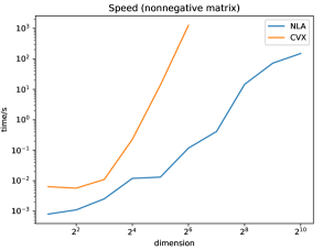
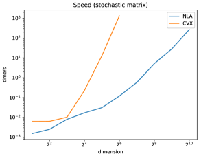
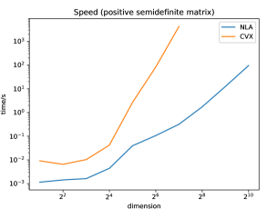
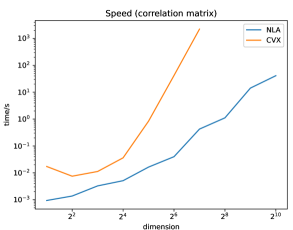
6.1. Speed

For each dimension $n=2^{d}$, we repeat our runs ten times and compare average time taken to reach a prespecified forward error. The default precisions of cvx are reltol = abstol = feastol = 1e-8 for ecos and eps_rel = eps_abs = 1e-4 for scs; we scale these parameters by the dimension of the matrix $n$. We record the final forward error of cvx and run Algorithm 5 until it achieves the same forward error. From Figure 1, Algorithm 5 outperforms cvx significantly in speed for large $n$. Indeed, the range of dimensions is limited by cvx, which fails to converge for large $n$. To get a rough idea, for $n=2^{7}$, cvx took about half an hour when Algorithm 5 took less than a second. For $n=2^{8}$ and beyond, cvx did not converge within 24 hours.

Figure 1. Speed of Algorithm 5 versus cvx.

These results are within expectation: in convex optimization, these problems are transformed to convex quadratic programs or semidefinite programs; both require at least $O(n^{4})$ operations per iteration, which is prohibitive for large $n$. In our Algorithm 5 and its two-projection variant (4.21), the dominating cost is the projection onto $\mathcal{S}$ — this is essentially free for nonnegative and stochastic matrices, requiring only $O(n^{2})$ operations per iteration; for correlation and positive semidefinite matrices, projections require around $O(n^{3})$ operations per iteration.

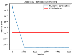
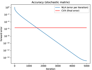
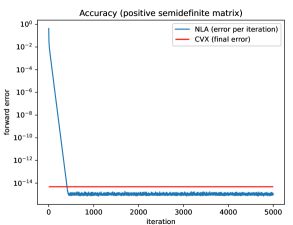
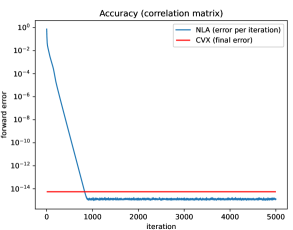
6.2. Accuracy

Here we compare the minimum possible forward error each method can achieve. We set $n=32$ as cvx may fail to converge in a reasonable amount of time for larger values of $n$. We set cvx to its maximum allowed precisions, reltol = abstol = feastol = 1e-16 for ecos and eps_rel = eps_abs = 1e-16 for scs, and record its final forward error. Then we run Algorithm 5 for 5,000 iterations and record its forward error at each iteration. Note that it is not meaningful to make iterationwise comparisons here as the two algorithms are entirely different. From Figure 2, we see that Algorithm 5 reaches beyond the maximum possible accuracy of cvx in every case. The linear convergence rate in Theorem 4.3 is also evident from these plots.

Figure 2. Accuracy of Algorithm 5 versus cvx. Here the red lines indicate the level of maximum possible accuracy of cvx.

7. Conclusion

Likely because of the increasing awareness of convex optimization as a potent tool in many areas, there has been a tendency to apply general purpose convex optimization methods to any convex problem. However convex problems like those considered in this article often have more structures than mere convexity. We show that approaching such problems through numerical linear algebra in the spirit of [11, 12, 15, 16, 17, 18, 20, 27, 30] can sometimes lead to better results, and has the advantage of working for the occasional nonconvex problem like (1.1).

Acknowledgment

The first author thanks Bartolomeo Stellato for helpful discussions.