CacheQL: Quantifying and Localizing Cache Side-Channel Vulnerabilities in Production Software

Abstract

Cache side-channel attacks extract secrets by examining how victim software accesses cache. To date, practical attacks on cryptosystems and media libraries are demonstrated under different scenarios, inferring secret keys and reconstructing private media data such as images.

This work first presents eight criteria for designing a full-fledged detector for cache side-channel vulnerabilities. Then, we propose CacheQL, a novel detector that meets all of these criteria. CacheQL precisely quantifies information leaks of binary code, by characterizing the distinguishability of logged side channel traces. Moreover, CacheQL models leakage as a cooperative game, allowing information leakage to be precisely distributed to program points vulnerable to cache side channels. CacheQL is meticulously optimized to analyze whole side channel traces logged from production software (where each trace can have millions of records), and it alleviates randomness introduced by cryptographic blinding, ORAM, or real-world noises.

Our evaluation quantifies side-channel leaks of production cryptographic and media software. We further localize vulnerabilities reported by previous detectors and also identify a few hundred new leakage sites in recent OpenSSL (ver. 3.0.0), MbedTLS (ver. 3.0.0), Libgcrypt (ver. 1.9.4). Many of our localized program points are within the pre-processing modules of cryptosystems, which are not analyzed by existing works due to scalability. We also localize vulnerabilities in Libjpeg (ver. 2.1.2) that leak privacy about input images.

1 Introduction

Cache side channels enable confidential data leakage through shared data and instruction caches. Attackers can recover program secrets like secret keys and user inputs by monitoring how victim software accesses cache units. Exploiting cache side channels has been shown particularly effective for cryptographic systems such as AES, RSA, and ElGamal [25, 53]. Recent attacks show that private user data including images and text can be reconstructed [62, 26, 66].

Both attackers and software developers are in demand to quantify and localize software information leakage. It is also vital to precisely distribute information leaks toward each vulnerable program point, given that exploiting program points that leak more information can enhance an attacker’s success rate. Developers should also prioritize fixing the most vulnerable program points. Additionally, cyber defenders are interested in assessing subtle information leaks over cryptosystems already hardened by mitigation techniques (e.g., blinding). Nevertheless, most existing cache side channel detectors focus exclusively on qualitative analysis, determining whether programs are vulnerable without quantifying information that these flaws may leak [57, 56, 59, 12, 66]. Given the complexity of real-world cryptosystems and media libraries, scalable, automated, and precise vulnerability localization is lacking. As a result, developers may be likely reluctant (or unaware) to remedy vulnerabilities discovered by existing detectors. As shown in our evaluation (Sec. 8), attack vectors in production software are underestimated.

This work initializes a comprehensive view on detecting cache side-channel vulnerabilities. We propose eight criteria to design a full-fledged detector. These criteria are carefully chosen by considering various important aspects like scalability. Then, we propose CacheQL, an automated detector for production software that meets all eight criteria. CacheQL quantifies information leakage via mutual information (MI) between secrets and side channels. CacheQL  recasts MI computation as evaluating conditional probability (CP), characterizing distinguishability of side channel traces induced by different secrets. This re-formulation largely enhances computing efficiency and ensures that CacheQL’s quantification is more precise than existing works. It also principally alleviates coverage issue of conventional dynamic methods.

We also present a novel vulnerability localization method, by formulating information leak via a side channel trace as a cooperative game among all records on the trace. Then, Shapley value [49], a well-established solution in cooperative game theory, helps to localize program points leaking secrets. We rely on domain observations (e.g., side channel traces are often sparse) to reduce the computing cost of Shapley value from $\mathcal{O}(2^{N})$ to roughly constant with nearly no loss in precision. CacheQL directly analyzes binary code, and captures both explicit and implicit information flows. CacheQL analyzes entire execution traces (existing works require traces to be cut to reduce complexity) and overcomes “non-determinism” introduced by noises or hardening techniques (e.g., cryptographic blinding, ORAM [25]).

We evaluate CacheQL using production cryptosystems including the latest versions (by the time of writing) of OpenSSL, Libgcrypt and MbedTLS. We also evaluate Libjpeg by treating user inputs (images) as privacy. To mimic debugging [57], we collect memory access traces of target software using Intel Pin as inputs of CacheQL. We also mimic automated real attacks in userspace-only scenarios, where highly noisy side channel logs are obtained via Prime+Probe [53] and fed to CacheQL. CacheQL analyzed 10,000 traces in 6 minutes and found hundreds of bits of secret leaks per software. These results confirm CacheQL’s ability to pinpoint all known vulnerabilities reported by existing works [56, 59] and quantify those leakages. CacheQL also discovers hundreds of unknown vulnerable program points in these cryptosystems, spread across hundreds of functions never reported by prior works. Developers promptly confirmed representative findings of CacheQL. Particularly, despite the adoption of constant-time paradigms to harden sensitive components, cryptographic software is not fully constant-time, whose non-trivial secret leaks are found and quantified by CacheQL. CacheQL reveals the pre-process modules, such as key encoding/decoding and BIGNUM initialization, can leak many secrets and affect all modern cryptosystems evaluated. In summary, we have the following contributions:

• We propose eight criteria for systematic cache side-channel detectors, considering various objectives and restrictions. We design CacheQL, satisfying all of them;

• CacheQL reformulates mutual information (MI) with conditional probability (CP), which reduces the computing error and cost efficiently. It then estimates CP using neural network (NN). Our NN can properly handle lengthy side channel traces and analyze secrets of various types. Moreover, it does not require manual annotations of leakage in training data;

• CacheQL further uses Shapley value to localize program points leaking secrets by simulating leakage as a cooperative game. With domain-specific optimizations, Shapley value, which is computational infeasible, is calculated with a nearly constant cost;

• CacheQL identifies subtle leaks (even with RSA blinding enabled), and its correctness has theoretical guarantee and empirical supports. CacheQL also localizes all vulnerable program points reported by prior works and hundreds of unknown flaws in the latest cryptosystems. Our representative findings are confirmed by developers. It illustrates the general concern that BIGNUM and pre-processing modules are largely leaking secrets and undermining recent cryptographic libraries.

Research Artifact. To support follow-up research, we release the code, data, and all our findings at https://github.com/Yuanyuan-Yuan/CacheQL [4].

2 Background & Motivating Example

Application Scope. CacheQL is designed as a bug detector. It shares the same design goal with previous detectors [57, 21, 56, 59, 60], whose main audiences are developers who aim to test and “debug” software. CacheQL is incapable of synthesizing proof-of-concept (PoC) exploits and is hence incapable of launching real attacks. In general, exploiting cache side channels in the real world is often a multi-step procedure [37] that involves pre-knowledge of the target systems and manual efforts. It is challenging, if not impossible, to fully automate the process. For instance, exploitability may depend on the specific hardware details [39, 37, 64], and in cloud computing, the success of co-residency attacks denotes a key pre-condition of launching exploitations [69]. These aspects are not considered by CacheQL which performs software analysis. Given that said, we evaluate CacheQL by quantifying information leaks over side channel traces logged by standard Prime+Probe attack, and as a proof of concept, we extend CacheQL to reconstruct secrets/images with reasonable quality over logged traces (see details in Appx. C). We believe these demonstrations show the potential and extensibility of CacheQL in practice.

Threat Model. Aligned with prior works in this field [6, 21, 57, 56, 12], we assume attackers share the same hardware platforms with victim software. Attackers can observe cache being accessed when victim software is running. Attackers can log all cache lines (or other units) visited by the victim software as a side channel trace [37, 64].

Given a program $g$, we define the attacker’s observation, a side channel trace, as $o\in O$ when $g$ is executing $k\in K$. $O$ and $K$ are sets of all observations and secrets. $K$ can be cryptographic keys or user private inputs like photos. We consider a “debug” scenario where developers measure leakage when $g$ executes $k$. Aligned with prior works [59, 60], we assume that developers can obtain noise-free $o$, e.g., $o$ is execution trace logged by Pin. We also assume developers are interested in assessing leaks under real attacks. Indeed, OpenSSL by default only accepts side channel reports exploitable in real scenarios [3]. We thus also launch standard Prime+Probe attack to log cache set accesses. We aim to quantify information in $k$ leaked via $o$. We also analyze leakage distribution across program points to localize flaws. Developers can prioritize patching vulnerabilities leaking more information.

Two Vulnerablities: Secret-Dependent Control Branch and Data Access. Our threat model focuses on two popular vulnerability patterns that are analyzed and exploited previously, namely, secret-dependent control branch (SCB) and secret-dependent data access (SDA) [38, 21, 22, 57, 56, 12, 6]. SDA implies that memory access is influenced by secrets, and therefore, monitoring which data cache unit is visited may likely reveal secrets [64]. SCB implies that program branches are decided by secrets, and monitoring which branch is taken via cache may likely reveal secrets [38]. CacheQL captures both SCB and SDA, and it models secret information flow. That is, if a variable $v$ is influenced (“tainted”) by secrets via either explicit or implicit information flow, then control flow or data access that depends on $v$ are also treated as SCB and SDA. The definition of SDA/SCB is standard and shared among previous detectors [57, 21, 56, 59, 60].

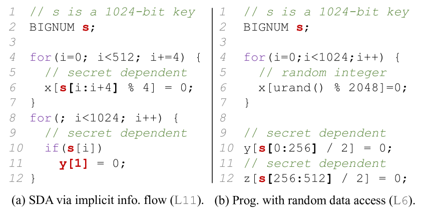
Figure 1: Two pseudocode code of secret leakage. The secrets are 1024-bit keys. s[i:j] are bits between the $i$-th (included) and $j$-th bit (excluded).

Detecting SDA Using CacheQL. Consider two vulnerable programs depicted in Fig. 1. In short, two program points in Fig. 1(a) have 128 (L6) and 512 (L11) memory accesses that are secret-dependent (i.e., SDA). Developer can use Pin to log one memory access trace $o$ when executing Fig. 1(a), and by analyzing $o$, CacheQL reports a total leakage of 768 bits. CacheQL further apportions the SDA leaked bits as: 1) 2 bits for each of 128 memory accesses at L6, and 2) 1 bit for each of 512 memory accesses at L11. For Fig. 1(b), two array lookups at L10 and L12 depend on the secret. Given a memory access trace $o$, CacheQL quantifies the leakage as 510 bits and apportions 255 bits for each SDA. We discuss technical details of CacheQL in Sec. 4, Sec. 5, and Sec. 6.

Comparison with Existing Quantitative Analysis. MicroWalk [60] measures information leakage via mutual information (MI). However, we find that its output is indeed mundane Shannon entropy rather than MI over different program execution traces, since both key and randomness like blinding can differ traces. MicroWalk has two computing strategies: whole-trace and per-instruction. For Fig. 1(b), MicroWalk reports 1024 leaked bits using the whole-trace strategy. The per-instruction strategy localizes three leakage program points, where each point leaks 1024 (L6), 255 (L10), and 255 (L12) bits, respectively. However, it is clear that those 1024 memory accesses at L6 are decided by non-secret randomness. Thus, both quantification and localization are inaccurate. Abacus [6] uses trace-based symbolic execution to measure leakage at each SDA, by estimating number of different secrets (s) that induces the access of different cache units. No implicit information flow is modelled, thereby omitting to “taint” the memory access at L11 of Fig. 1(a). Abacus quantifies leakage of Fig. 1(a) over $o$ as 256 bits, since it only finds SDA at L6.

Program points may have dependencies. For instance, one branch may have its information leaked in its parent branch, and therefore, separately adding them together largely over-estimates the leakage: Abacus outputs a total leakage of 413.6 bits in AES-128, despite its 128-bit key length. CacheQL precisely calculates the leakage as 128.0 bits (Sec. 8.2.1). Also, some static analyses [21, 22, 15] have limited scalability due to heavyweight abstract interpretation or symbolic execution. Real-world cryptosystems and media software are complex, with millions of records per side channel trace. In addition, they are often unable to localize vulnerable points.

Table 1: Benchmarking criteria for side channel detectors. ✓, $\Diamond$, ✗ denote support, partially support, and not support.

	CacheAudit [21, 22]	CacheD [57]	CaSym [12]	CacheS [56]	Abacus [6]	CHALICE [15]	DATA [59, 58]	MicroWalk [60]	CANAL [52]	Manifold [66]	CacheQL
	✗	✗	✗	✗	✗	✗	✗	✗	✗	✓	✓
	✗	✗	✗	✗	✗	✗	$\Diamond$	✗	✗	✗	✓
	✗	✓	✗	✓	✓	✗	✓	✓	✗	✓	✓
	$\Diamond$	✗	✗	✗	$\Diamond$	$\Diamond$	✗	$\Diamond$	✗	✗	✓
	✗	✓	✓	✓	✓	✗	✓	$\Diamond$	✓	✓	✓
	✗	✗	✗	✗	✗	✗	✗	✗	✗	$\Diamond$	✓
	✗	✗	✗	✗	✗	✗	✓	✓	✗	✓	✓
	✓	✗	✗	✗	✗	✓	$\Diamond$	$\Diamond$	✓	✓	✓

3 Related Works & Criteria

We propose eight criteria for a full-fledged detector. Accordingly, we review related works in this field and assess their suitability. Sec. 8.3 empirically compares them with CacheQL. Also, many studies launch cache analysis on real-time systems and estimate worst-case execution time (WCET) [16, 35, 36, 43]; we omit those studies as they are mainly for measurement, not for vulnerability detection.

Execution Trace vs. Cache Attack Logs. Most existing detectors [57, 56, 12] assume access to execution traces. In addition to recording noise-free execution traces (e.g., via Intel Pin), considering real cache attack logs is equally important. Cryptosystem developers often require evidence under real-world scenarios to issue patches. For instance, OpenSSL by default only accepts side channel reports if they can be successfully exploited in real-world scenarios [3]. In sum, we advocate that a side channel detector should  analyze both execution traces and real-world cache attack logs.

Deterministic vs. Non-deterministic Observations. Deterministic observations imply that, for a given secret, the observed side channel is fixed. Decryption, however, may be non-deterministic due to various masking and blinding schemes used in cryptosystems. Furthermore, techniques like ORAM [25] can generate non-deterministic memory accesses and prevent information leakage. Thus, memory accesses or executed branches may differ between executions using one secret. Nearly all previous works [57, 6, 56, 12] only consider deterministic side channels, failing to analyze the protection offered by blinding/ORAM and may overestimate leaks (not just keys, blinding/ORAM also change side channel observations). We suggest that a detector should  analyze both deterministic and non-deterministic observations. CacheQL uses statistics to quantify information leaks from non-deterministic observations, as explained in Sec. 4.4.

Analyze Source Code vs. Binary. A detector should typically analyze software in executable format. This allows the analysis of legacy code and third-party libraries. More importantly, by analyzing assembly code, low-level details like memory allocation can be precisely considered. Studies [22, 51] reveal that compiler optimizations could introduce side channels not visible in high-level code representations. Thus, we argue that detectors should  be able to analyze program executables.

Quantitative vs. Qualitative. Qualitative detectors decide whether software leaks information and pinpoint leakage program points [57, 56, 12]. Quantitative detectors further quantify leakage from each software execution [21, 15, 22], or at each vulnerable program point [6, 60]. We argue that a detector should  deliver both qualitative and quantitative analysis. Developers are reluctant to fix certain vulnerabilities, as they may believe those defects leak negligible secrets [6]. However, identifying program points that leak large amounts of data can push developers to prioritize fixing them. To clarify, though quantitative analysis was previously deemed costly [31], CacheQL features efficient quantification.

Localization. Along with determining information leaks, localizing vulnerable program points is critical. Precise localization helps developers debug and patch. Therefore, a detector should  localize vulnerable program points leaking secrets. Most static detectors struggle to pinpoint leakage points [21, 22], as they measure the number of different cache statuses to quantify leakage. Trace-based analysis, including CacheQL, can identify leakage instructions on the trace that can be mapped back to vulnerable program points [57, 6].

Key vs. Private Media Data. Most detectors analyze cryptosystems to detect key leakage [57, 21, 6]. Recent side channel attacks have targeted media data [62, 26]. Media data like images used in medical diagnosis may jeopardize user privacy once leaked. We thus advocate detectors to  analyze leakage of secret keys and media data. Modeling information leakage of high-dimensional media data is often harder, because defining “information” contained in media data like images may be ambiguous. CacheQL models image holistic content (rather than pixel values) leakage using neural networks.

Scalability: Whole Program/Trace vs. Program/Trace Cuts. Some prior trace-based analyses rely on expensive techniques (e.g., symbolic execution) that are not scalable. Given that one execution trace logged from cryptosystems can contain millions of instructions, existing works [57, 6] require to first cut a trace and analyze only a few functions on the cutted trace. Prior static analysis-based works may use abstract interpretation [21, 56], a costly technique with limited scalability. Only toy programs [21] or a few sensitive functions are analyzed [56, 22, 12]. This explains why most existing works overlook “non-deterministic” factors like blinding (criterion ), as blinding is applied prior to executing their analyzed program/trace cuts. Lacking whole-program/trace analysis limits the study scope of prior works. CacheQL can analyze a whole trace logged by executing production software, and as shown in Sec. 8, CacheQL  identifies unknown vulnerabilities in pre-processing modules of cryptographic libraries that are not even covered by existing works due to scalability. In sum, we advocate that a detector should be  scalable for whole-program/whole-trace analysis.

Implicit and Explicit Information Flow. Explicit information flow primarily denotes secret data flow propagation, whereas implicit information flow models subtle propagation by using secrets as code pointers or branch conditions [48]. Considering implicit information flow is challenging for existing works based on static analysis due to scalability. They thus do not fully analyze implicit information flow [57, 56, 12, 6]. We argue a detector should  consider both implicit and explicit information flow to comprehensively model potential information leaks. CacheQL delivers an “end-to-end” analysis and identifies changes in the trace due to either implicit or explicit information flow propagation of secrets.

Comparing with Existing Detectors. Table 1 compares existing detectors and CacheQL to the criteria. Abacus and MicroWalk cannot precisely quantify information leaks in many cases, due to either lacking implicit information flow modeling or neglecting dependency among leakage sites (hence repetitively counting leakage). CacheAudit only infers the upper bound of leakage. Thus, they partially satisfy . MicroWalk quantifies per-instruction MI to localize vulnerable instructions, whose quantified leakage per instruction, when added up, should not equal quantification over the whole-trace MI (its another strategy) due to program dependencies. Also, MicroWalk cannot differ randomness (e.g., blinding) with secrets. It thus partially satisfies .

DATA [59, 58] launches trace differentiation and statistical hypothesis testing to decide secret-dependency of an execution trace. Similar as CacheQL, DATA can also analyze non-deterministic traces. Nevertheless, we find that DATA, by differentiating traces to detect leakage, may manifest low precision, given it would neglect secret leakage if a cryptographic module also uses blinding. It thus partially satisfies . More importantly, DATA does not deliver quantitative analysis.

Recent research attempts to reconstruct media data like private user photos from side channels [66, 34, 61]. In Table 1, we compare CacheQL with Manifold [66], the latest work in this field. Manifold leverages manifold learning to infer media data. Manifold learning is not applicable to infer secret keys (as admitted in [66]): unlike media data which contain perception constraints retained in manifold [28], each key bit is sampled independently and uniformly from 0 or 1. It thus partially fulfills . CacheQL is the first to quantify information leaks over cryptographic keys and media data.

Implicit information flow () is not tracked by most existing static analyzers. Analyzing implicit information flow requires considering more program statements and data/control flow propagations, which often largely increases the code chunk to be analyzed. This introduces extra hurdles for static analysis-based approaches. DATA and MicroWalk also do not systematically capture implicit information flow. DATA/MicroWalk first align traces and then compare aligned segments, meaning that they can overlook holistic differences (unalignment) on traces. CacheQL satisfies as it directly observes and analyzes changes in the side channel traces. Given any information flow, either explicit or implicit, can differ traces, CacheQL captures them in a unified manner. Nevertheless, it is evident that the implicit information flow cannot be captured by CacheQL unless it is covered in the dynamic traces.

Clarification. These criteria’s importance may vary depending on the situations. Having only some of these criteria implemented is not necessarily “bad,” which may suggest that the tool is targeted for specific use cases. Analyzing private image leakage () may not be as important as others, especially for cryptosystem developers. We consider image leakage because recent works [62, 26, 66] consider recovering private media data. We present eight criteria for building full-fledged side-channel detectors. The future development of detectors can refer to this paper and prioritize/select certain criteria, according to their domain-specific need. Also, we clarify that in parallel to research works that detect side channel leaks, another line of approaches (i.e., static verification) aims at deriving precise, certified guarantees [21, 20].

As clarified above, CacheQL can analyze real attack logs () and media data (). However, for the sake of presentation coherence, we discuss them in Sec. 9. In the rest of the main paper, we explain the design and findings of CacheQL using Pin-logged traces from cryptosystems.

4 Quantifying Information Leakage

Overview. This section discusses quantitative measurement of information leaks over side channel observations. We start with preliminaries in Sec. 4.1. The overview of our approach is illustrated in Fig. 2. Sec. 4.2 introduces MI computation via Point-wise Dependence (PD). Then, Sec. 4.3 recasts calculating PD into computing conditional probability (CP). CacheQL employs parameterized neural networks $\mathcal{F}_{\theta}$ (see Sec. 5) to estimate CP, which is carefully designed to quantify leakage of keys and private images from extremely lengthy side channel traces. The error of estimating CP with $\mathcal{F}_{\theta}$ is bounded by a negligible $\epsilon$. In contrast, prior works use marginal probability (MP) to estimate MI. CP outperforms MP in terms of lower cost, fewer errors, and better coverage, as compared in Sec. 4.3. In Sec. 4.4, we extend the pipeline in Fig. 2 to handle non-deterministic side channel traces.

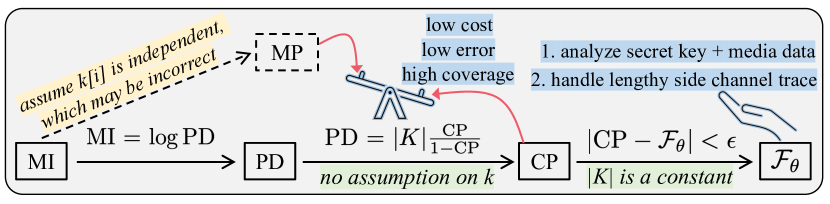
Figure 2: Overview. $|K|$ is the total number of possible keys. $|K|$ is assumed as known to detectors by all existing quantification tools including CacheQL.

4.1 Problem Setting

In general, side channel analysis aims to infer $k$ from $o$. The information leak of $K$ in $O$ can be defined as their MI:

$${I(K;O)=H(K)-H(K|O),}$$ (1)

where $H(\cdot)$ denotes the entropy of an event. According to Shannon’s information theory, $I(K;O)$ describes how much information about $K$ can be obtained by observing $O$. Consider the program in Fig. 3(a), where the probability of correctly guessing each $k\in K$ (i.e., $\texttt{s}\in\{\texttt{0},\texttt{1},\texttt{2},\texttt{3}\}$), without any observation, is $\frac{1}{4}$. Thus, $H(K)$ = $-\log\frac{1}{4}$ = $2$ bits. Nevertheless, the observation $o$ = $a[0]$ (L6) indicates that $k$ must be “0” (i.e., the probability is $1$), thus, $H(K|o$=$a[0])$ = $-\log 1$ = $0$. Therefore, $a[0]$ leaks 2 bits of information. Similarly, the memory access $b[0]$ (L9) leaks $\log\frac{4}{3}$ bits of information since $H(K|o$=$b[0])$ = $-\log\frac{1}{3}$ = $\log 3$. Ideally, a secure program should have $H(K)$ = $H(K|O)$, indicating no information in $K$ can be obtained from $O$. We continue discussing Fig. 3(b) in Sec. 4.3.

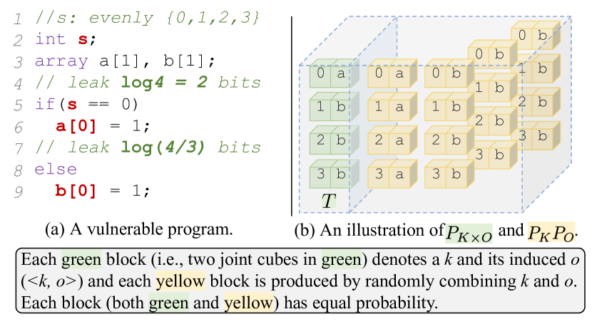
Figure 3: Quantification of side channel leaks.

4.2 Computing MI via PD

Following Eq. 1, let $k$ and $o$ be random variables whose probability density functions (PDF) are $p(k)$ and $p(o)$. The MI $I(K;O)$ can be represented in the following way,

$$I(K;O)=\int\int_{K\times O}p(k,o)\log\frac{p(k,o)}{p(k)p(o)}\mathrm{d}k\mathrm{d}o$$ (2)

$$=\mathbb{E}_{P_{K\times O}}\left[\log\frac{p(k,o)}{p(k)p(o)}\right]=\mathbb{E}_{P_{K\times O}}[\log c(k,o)],$$

where $p(k,o)$ is the joint PDF of $K$ and $O$, and $P_{K\times O}$ is the joint distribution. $c(k,o)=\frac{p(k,o)}{p(k)p(o)}$ denotes point-wise dependency (PD), measuring discrepancy between the probability of $k$ and $o$’s co-occurrence and the product of their independent occurrences. Accordingly, $\log c(k,o)$ denotes the point-wise mutual information (PMI).

The MI of $K$ and $O$, by definition, is the expectation of PMI. That is, Eq. 2 measures the dependence retained in the joint distribution (i.e., $\langle k,o\rangle\sim P_{K\times O}$) relative to the marginal distribution of $K$ and $O$ under the assumption of independence (i.e., $\langle k,o\rangle\sim P_{K}P_{O}$, where $P_{K}$ and $P_{O}$ are marginal distributions of $K$ and $O$). When $K$ and $O$ are independent, we have $p(k,o)$ = $p(k)$$\cdot$$p(o)$ and $\frac{p(k,o)}{p(k)p(o)}$ is $1$, thus, the leakage is $\log 1$=$0$. Nevertheless, whenever $o$ leaks $k$, $k$ and $o$ should co-occur more often than their independent occurrences, and therefore, $c(k,o)>1$ and $\log c(k,o)>0$.

Eq. 2 illustrates two aspects for quantitatively computing information leakage: 1) PMI $\log c(k$=$k^{*},o$=$o^{*})$, denoting per trace leakage for a specific $k^{*}$ and its corresponding $o^{*}$, and 2) MI $I(K;O)$, denoting program-level leakage over all possible secrets $k\in K$. To compute $I(K;O)$, we average PMI over a collection of $\langle k,o\rangle$, where sample-mean offers an unbiased estimation for the expectation $\mathbb{E}(\cdot)$ of a distribution [14].

Comparison with Prior Works. Abacus [6] launches symbolic execution on Pin-logged execution traces. It makes a strong assumption that $k$ is uniformly distributed, i.e., $p(k$=$k^{*})$ = $\frac{1}{|K|}$. It also assumes that each trace must be deterministic, such that $p(k$=$k^{*},o$=$o^{*})$ = $p(k$=$k^{*})$ for a given $o^{*}$ and its corresponding $k^{*}$. This way, approximating MI in Eq. 2 is recasted to estimating the marginal probability (MP) $p(o$=$o^{*})$. At a secret-dependent control transfer or data access point $l$, Abacus finds all $k\in K^{\prime}$ that cover $l$. The leakage at $l$ is computed as $-\log p(o$=$o^{*})$ = $-\log(\frac{|K^{\prime}|}{|K|})$. Deciding $|K^{\prime}|$ via constraint solving is costly, and therefore, Abacus uses sampling to approximate $|K^{\prime}|$. Nevertheless, estimating MP with sampling is unstable and error-prone (see Sec. 4.3). MicroWalk also samples $k$ to estimate MP; it thereby has similar issues. CacheAudit quantifies program-wide leakage. Using abstraction interpretation, it only analyzes small programs or code fragments, and it infers only leak upper bound. CacheQL precisely computes PMI/MI via PD and localizes flaws. We now introduce estimating PD.

4.3 Estimating PD $c(k,o)$ via CP

Because PD makes no assumption on the secret’s distribution, our approach can infer different types of secrets (e.g., key or images). We denote $k$ as a general representation of one secret, and for simplicity, we write $p(k$=$k^{*})$ as $p(k^{*})$ in followings. The same applies for $o$ and $o^{*}$. $o^{*}$ is one side channel observation produced by $k^{*}$. However, $o^{*}$ may not be the only one, given randomness like blinding can also induce different observations even with a fixed $k^{*}$. We now recast computing PD over deterministic side channels as estimating conditional probability (CP) via binary classification [54].

4.3.1 Transforming PD to CP

Let $T$ depict that a pair $\langle k,o\rangle$ co-occurs (i.e., positive pair $\langle k,o\rangle\sim P_{K\times O}$). Let $F$ denote that $k$ and $o$ in $\langle k,o\rangle$ occur independently (i.e., negative pair $\langle k,o\rangle\sim P_{K}P_{O}$). Therefore, $p(k^{*},o^{*})$ and $p(k^{*})p(o^{*})$ can be represented as the posterior PDF $p(k^{*},o^{*}|T)$ and $p(k^{*},o^{*}|F)$, respectively. According to Bayes’ Theorem, PD $c(k^{*},o^{*})$ is re-expressed as

$${\text{PD}=\frac{p(k^{*},o^{*})}{p(k^{*})p(o^{*})}=\frac{p(k^{*},o^{*}|T)}{p(k^{*},o^{*}|F)}=\frac{p(F)}{p(T)}\frac{p(T|k^{*},o^{*})}{p(F|k^{*},o^{*})},}$$ (3)

where $p(T)$ and $p(F)$ are constants (decided by the analyzed software). Given $P_{K}P_{O}$ is produced by separating each pair in $P_{K\times O}$ and collecting random combinations of $k$ and $o$, $\frac{p(F)}{p(T)}$ equals to $|K|$. In practice, $P_{K\times O}$ is prepared by running the analyzed software with each $k^{*}$ and collecting the corresponding $o^{*}$. For the program in Fig. 3(a), Fig. 3(b) colors $P_{K\times O}$ and $P_{K}P_{O}$ in green and yellow. Since $\frac{p(F)}{p(T)}$ is unrelated to $k^{*}$ or $o^{*}$, $c(k^{*},o^{*})$ — representing leaked $k^{*}$ from $o^{*}$ — is only decided by CP $p(T|k^{*},o^{*})$. A larger CP indicates that more information is leaked.

$\bullet$ Example: We demonstrate this transformation using Fig. 3: for $k$=“0” and $o$=$a[0]$, fetching a block of $\langle\texttt{0},\texttt{a}\rangle$ from Fig. 3(b) has a $50\%$ chance of selecting the green one (in the upper-left corner). That is, CP=$p(T|\text{``{0}''},a[0])$=$0.5$, and therefore, $p(T|\text{``{0}''},a[0])$= $p(F|\text{``{0}''},a[0])$. Since $\frac{p(F)}{p(T)}$=$4$, Eq. 3 yields $4\times\frac{0.5}{0.5}=4$, and therefore, $\log c(k,o)$ in Eq. 2 yields $\log 4=2$ bits, equaling the leakage result computed in Sec. 4.1.

4.3.2 Advantages of CP vs. Marginal Probability (MP)

CP captures what factors make $o^{*}$, which corresponds to $k^{*}$, distinguishable from other $o$. By observing both dependent and independent $\langle k,o\rangle$ pairs, CacheQL measures the leakage via describing how the distinguishability between different $o$ is introduced by the corresponding $k$. It is principally distinct with existing quantitative analysis [6, 21, 60]. Abacus and MicroWalk approximate MP $p(o^{*})$ via sampling, which has the following three limitations compared with CP.

Computing Cost. Estimating CP is an one-time effort over a collection of $\langle k,o\rangle$ pairs. Estimating MP, however, has to re-perform sampling for each $\langle k,o\rangle$. Note that the cost for CP to estimate over the collection of $\langle k,o\rangle$ and each re-sampling of MP is comparable. Thus, MP is much more costly.

Estimation Error. Recall that for a leakage program point $l$, Abacus finds all $k\in K^{\prime}$ that cover $l$ via constraint solving and denotes the leakage as $-\log(\frac{|K^{\prime}|}{|K|})$. Suppose it observes the first for loop in Fig. 1(a) has 128 consecutive accesses to $x[0]$. To quantify the leakage, Abacus constructs the symbolic constraint $(s[0$:$4]\%4==0)\land\ldots\land(s[508$:$512]\%4==0)$. Nevertheless, sampling one key that satisfies this constraint has only an extremely low probability of $(\frac{1}{4})^{128}$. That is, the MP can be presumably underestimated when $|K^{\prime}|$ is small. Thus, the leaked information can be largely overestimated via $-\log(\frac{|K^{\prime}|}{|K|})$. MicroWalk observes $o^{*}$’s frequency by sampling different $k$; it thus has similar issues. Worse, once $o^{*}$ is influenced by randomness like blinding, no $o^{*}$ would be identical (non-replicability). Thus, it will incorrectly regard $p(o^{*})$ as $\frac{1}{|K|}$ and report $\log|K|$ leaked bits (i.e., equals to the key length). In contrast, Eq. 3 is free from this issue: even $o^{*}$ is only produced by processing one or a few $k$, CacheQL directly characterizes PD via CP $p(\cdot|k^{*},o^{*})$.

Overall, CP reflects: 1) the portion of records in $o^{*}$ affected by its $k^{*}$ [54], and 2) to what extent $k^{*}$ affects each record in $o^{*}$ (see Example below). Further, since any difference on $o^{*}$, whether due to explicit or implicit information flows, contributes to distinguishing $o^{*}$ from the rest $o\in O$, CacheQL takes both explicit and implicit flows into consideration.

$\bullet$ Example: Consider the memory accesses at L10 and L12 of the program in Fig. 1(b) and suppose $o^{*}$ is “$y[0]$, $z[0]$”. To estimate the leakage over $o^{*}$ via MP, it requires sampling keys where $s[0$:$256]$ constitutes either 1 or 0, so do the second 256 bits, which results in a total of 4 cases for $s[0$:$512]$. $s[0$:$512]$ has $2^{512}$ cases, denoting a large search space. Nevertheless, CP can infer the leakage by only observing that, the first record in $o$ increases “1” (i.e., distinguishable from other $o$) whenever $s[0$:$256]$ increases 2 (with no need to simultaneously consider $s[256$:$512]$). The same applies to the second 256 bits.

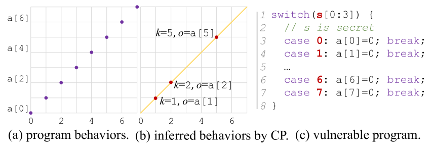
Figure 4: A schematic view of how the coverage issue of dynamic methods is alleviated via CP when quantifying leaks.

Coverage Issue. CacheQL, by using CP, principally alleviates the coverage issue of conventional dynamic methods. Consider the program in Fig. 4(c), CacheQL can quantify the 8 SDA without covering all paths, since CP captures how $o$ changes with $k$. As shown in Fig. 4(b), covering a few cases is sufficient to know that $o$ increases “one” (e.g., $a[0]\rightarrow a[1]$) when $k$ increases one (e.g., $0\rightarrow 1$), thus inferring program behavior in Fig. 4(a). Prior dynamic methods need to fully cover all paths to infer the program behavior and quantify the leaks, which is hardly achievable in practice.

4.3.3 Obtaining CP $p(T|k,o)$ via Binary Classification

We show that performing probabilistic classification can yield CP. In particular, we employ neural networks $\mathcal{F}_{\theta}$ (parameterized by $\theta$) to classify a pair of $\langle k,o\rangle$, whose associated confidence score is $p(T|k,o)$. Details of $\mathcal{F}_{\theta}$ are in Sec. 5.

Using neural networks (NN) to estimate MI is not our novelty [54, 8]. However, we deem NN as particularly suitable for our research context for three reasons: 1) non-parametric approaches, as in [24], suffer from “curse of dimensionality” [10, 11]. They are thus infeasible, as even the AES-128 key is 128-dimensional. NN shows encouraging capability of handling high-dimension data (e.g., images with thousands of dimensions). 2) Recent works show that NN can effectively process lengthy but sparse data, including side channel traces where only a few records out of millions are informative and leaking program secrets [66, 34, 61]. 3) It’s generally vague to define “information” in media data. For instance, a $64\times 64$ image may retain the same information as a $32\times 32$ version from human perspective since the content is unchanged. Recent research [66] shows that high-dimensional media data have perceptual constraints which implicitly encode image “information.” NNs are currently widely used to process media data and extract critical information for comprehension.

4.4 Handling Non-determinism

In practice, due to hardening schemes like RSA blinding and ORAM, side channel observations can be non-deterministic, where memory access traces may vary during different runs despite the same key is used. As discussed in Table 1 (i.e., ), however, non-determinism is not properly handled in previous (quantitative) analysis.

Generalizability. For deterministic side channels, only $k$ induces changes of $o$. Fitting $\mathcal{F}_{\theta}$ on enough $\langle k,o\rangle$ pairs from $P_{K\times O}$ and $P_{K}P_{O}$ can capture distinguishability for quantification. In contrast, for non-deterministic side channels, the differences between $o$ may be due to random factors, not only $k$. Therefore, in addition to distinguishability between $\langle k,o\rangle$ pairs, we also need to consider generalizability to alleviate over-estimation caused by random differences.

In statistics, cross-validation is used to test generalizability. Here, we propose a simple yet effective method by using a de-bias term with cross-validation to prune non-determinism in the estimated PD. We first mix $\langle k,o\rangle$ from $P_{K\times O}$ and $P_{K}P_{O}$ and split them into non-overlapping groups. Then, we assess if the distinguishability over one group applies to the others.

PD Estimation via De-biasing. We first extend the PD computation in Eq. 3 to handle non-determinism. In Eq. 3, $F$ and $T$ are finite sets, and $p(F)/p(T)$ equals to $|K|$. Here, we conservatively assume that there exist infinite non-deterministic side channels. That is, $F$ is a set with infinite elements. We first require $m$ positive pairs $\langle k,o\rangle\sim P_{K\times O}$, dubbed as $T^{(m)}$. We also construct $m^{\prime}\leq m^{2}$ negative pairs (i.e., $\langle k,o\rangle\sim P_{K}P_{O}$), denoted as $F^{(m^{\prime})}$, by replacing $o$ (or $k$) of a pair from $P_{K\times O}$ with that of other random pairs. This way, PD defined in Eq. 3 is extended in the following form:

$${\text{PD}=\frac{\log|K|}{\log(m^{\prime}/m)}\log\frac{p(F^{(m^{\prime})})}{p(T^{(m)})}\frac{p(T|k^{*},o^{*})}{p(F|k^{*},o^{*})},}$$ (4)

where the $p(F^{(m^{\prime})})/p(T^{(m)})$ works as a de-bias term to assess the generalizability for non-deterministic side channels. We denote $p(T|k^{*},o^{*})/p(F|k^{*},o^{*})$ as the leakage ratio: a 100% ratio implies that all bits of the key are leaked whereas 0% ratio implies no leakage. Consider the following two cases:

$\bullet$ $\textit{Case}_{1}$: In case the differences between samples from $T^{(m)}$ and $F^{(m^{\prime})}$ are all introduced by random noise (i.e., each $o^{*}$ is independent of its $k^{*}$), the distinguishable factors should not be generalizable, and the above formula yields a zero leakage. To understand this, let our neural networks $\mathcal{F}_{\theta}$ identify each pair based on random differences, which is indeed equivalent to memorizing all pairs. This way, when it predicts the label of $\langle k,o\rangle$, the output simply follows the frequency of $T^{(m)}$ and $F^{(m^{\prime})}$. Therefore, given an unseen pair $\langle k^{*},o^{*}\rangle$, $\mathcal{F}_{\theta}$  has $p(T|k^{*},o^{*})/p(F|k^{*},o^{*})=p(T^{(m)})/p(F^{(m^{\prime})})$, and the estimated leakage is thus $\log\frac{p(F^{(m^{\prime})})}{p(T^{(m)})}\frac{p(T^{(m)})}{p(F^{(m^{\prime})})}=\log 1=0$.

$\bullet$ $\textit{Case}_{2}$: If $o^{*}$ depends on $k^{*}$, $p(T|k^{*},o^{*})$ would not merely follow the distribution of $T^{(m)}$ and $F^{(m^{\prime})}$, indicating a non-zero leakage. More importantly, de-biased by $p(F^{(m)})/p(T^{(m^{\prime})})$, quantifying leakage using Eq. 4 only retains differences related to $k$. This way, we precisely quantify leakage for non-deterministic side channels.

Implementation Consideration. To alleviate randomness in each $o^{*}$, we collect four observations $o_{i}^{*}$ by running software using $k^{*}$ for four times. By classifying all $\langle k^{*},o_{i}^{*}\rangle$ as positive pairs, $\mathcal{F}_{\theta}$ is guided to extract common characters shared by $o_{i}^{*}$ while neglecting randomness in each $o_{i}^{*}$. Also, considering un-optimized neural networks generally make prediction by chance (i.e., $p(T|k,o)=p(F|k,o)$), we let $m=m^{\prime}$.

5 Framework Design

Fig. 5 shows the pipeline of CacheQL, including three components: 1) a sparse encoder $\mathcal{S}$ for converting side channel traces $o^{*}$ into latent vectors, 2) a compressor $\mathcal{R}$ to shrink information in $o^{*}$, and 3) a classifier $\mathcal{C}$ that fits the CP in Eq. 3 via binary classification. We compute CP $p(T|k^{*},o^{*})$ using the following pipeline:

$$p(T|k^{*},o^{*})=\mathcal{F}_{\theta}(k^{*},o^{*})=\mathcal{C}(k^{*},\mathcal{R}(\mathcal{S}(o^{*}))),$$ (5)

where parameters of these three components are jointly optimized, i.e., $\theta=\theta_{\mathcal{S}}\cup\theta_{\mathcal{R}}\cup\theta_{\mathcal{C}}$.

Figure 5: The framework of CacheQL. $\langle k^{*},o^{*}\rangle$$\in$$P_{K\times O}$; it is labeled as $T$. In contrast, $\langle k^{\prime},o^{*}\rangle$$\in$$P_{K}P_{O}$ and is labeled as $F$.

The framework takes a tuple $\langle k,o\rangle$ as input. As introduced in Sec. 4.3, we label a tuple $\langle k,o\rangle$ as positive if $o$ is produced when the software is processing $k$. A tuple is otherwise negative. In Fig. 5, $\langle k^{*},o^{*}\rangle$ is positive and $\langle k^{\prime},o^{*}\rangle$ is negative.

$\mathcal{S}$: Encoding Lengthy and Sparse Side Channel Traces. According to our tentative experiments, naive neural networks perform poorly when analyzing real-world software due to the highly lengthy side channel traces. An $o$, obtained via Pin or cache attacks, typically contains millions of records, exceeding the capability of typical neural networks. ORAM can add dummy memory accesses, often resulting in a tenfold increase of trace length. Yuan et. al [66] found that side channel traces are generally sparse, with few secret-dependent records. It also has spatial locality: adjacent records on a trace often come from the same or related functions. Encoder $\mathcal{S}$ is inspired by [66]: to approximate the locality, we fold the trace into a matrix (see configurations in Sec. 8). We employ the design in [66] to construct $\mathcal{S}$ as a stack of convolutional NN layers. We find that our pipeline effectively extracts informative features from $o$.

$\mathcal{R}$: Shrinking Maximal Information. A side channel trace $o^{*}$ frequently contains information unrelated to secret $k^{*}$. Our preliminary study shows that directly bridging the latent vectors (outputs of $\mathcal{S}$) to $\mathcal{C}$ is difficult to train. This stage thereby compresses $\mathcal{S}$’s output in an information-dense manner. We propose that information in $o^{*}$, namely $H(o^{*})$, should never exceed $H(k^{*})$. Accordingly, we apply mathematical transformations $\mathcal{R}$ to confine the value range of $\mathcal{S}$’s outputs. We propose various transformations for media data and secret keys; details are in Appx. B. In short, $\mathcal{R}$ aids in retrieving secret-related information from side channels. As demonstrated in Appx. B, CacheQL effectively extracts facial attributes when estimating leakage of human photos.

$\mathcal{C}$: Optimizing Parameters via Classification. Let the parameter space be $\Theta$ and $\theta\in\Theta$. To train a neural network, we search for parameter $\theta^{\dagger}\in\Theta$ to maximize a pre-defined objective. As shown in Eq. 3, we recast leakage estimation as approximating CP $p(T|k,o)$, which is further formed as a classification task using $\mathcal{F}_{\theta}$. $\theta$ is updated by gradient-guided search in $\Theta$ to maximize the following objective:

$$\mathbb{E}_{P_{K\times O}}[\log\mathcal{F}_{\theta}(k,o)]+\mathbb{E}_{P_{K}P_{O}}[\log(1-\mathcal{F}_{\theta}(k,o))],$$ (6)

which is a standard binary cross-entropy loss over $P_{K\times O}$ and $P_{K}P_{O}$. Overall, this loss function compares the output of $\mathcal{F}_{\theta}$ to the ground truth, and it calculates the score that penalizes $\mathcal{F}_{\theta}$ based on its output distance from the expected value.

$\bullet$ Example: Consider the program in Fig. 3, in which we have $\langle\texttt{0},\texttt{a}\rangle$ labeled as $T$. To prepare $P_{K}P_{O}$, there is one $\langle\texttt{0},\texttt{a}\rangle$ marked as $F$ when randomly combining $k$ and $o$ separated from pairs in $P_{K\times O}$. Thus, $\mathcal{F}_{\theta}(\text{``{0}''},a[0])$ is simultaneously guided to output 1 and 0 with equal penalty. As expected, it eventually yields 0.5 to minimize the global penalty, which outputs a leakage of 4 bits (since $|K|=4$) following Eq. 7.

Computing PD. Let the optimized parameter be $\theta^{\dagger}$, our definition of PD in Eq. 3 is re-expressed in the following way to compute point-wise information leak of $k^{*}$ in its derived $o^{*}$:

$${c_{\theta^{\dagger}}(k^{*};o^{*})=|K|\frac{\mathcal{F}_{\theta^{\dagger}}(k^{*},o^{*})}{1-\mathcal{F}_{\theta^{\dagger}}(k^{*},o^{*})}}$$ (7)

Furthermore, we have the following program-level information leak assessment over $K$ and $O$.

$${I(K;O)=\mathbb{E}_{P_{K\times O}}\left[\log c_{\theta^{\dagger}}(k,o)\right]}$$ (8)

Approximation and Correctness. Having access to all samples from a distribution $P$ is difficult, if not impossible. As a common approximation, the objective in Eq. 6 is instead optimized over the empirical distribution $P^{(n)}$ produced by $n$ samples drawn from $P$. Thus, the estimated leakage becomes:

$${\hat{I}^{(n)}_{\theta^{\dagger}}(K;O)=\mathbb{E}_{P^{(n)}_{K\times O}}[\log\hat{c}_{\theta^{\dagger}}(k,o)].}$$ (9)

Despite we estimate MI for side channels, the skeleton for analyzing correctness can be adopted from prior works [54, 8], since all approaches involve optimizing parameterized neural networks. In particular, we prove that $\exists\theta^{\dagger}\in\Theta$,

$${|\hat{I}^{(n)}_{\theta^{\dagger}}(K;O)-I(K;O)|\leq\mathcal{O}(\sqrt{\log(1/\delta)/n}),}$$ (10)

with probability at least $1-\delta$ where $0<\delta<1$. We present detailed proofs in Appx. D.

6 Apportioning Information Leakage

We analyze how leakage over $\langle o^{*},k^{*}\rangle$ is apportioned among program points. This section models information leakage as a cooperative game among players (i.e., program points). Accordingly, we use Shapley value [49], a well-developed game theory approach, to apportion player contributions.

Overview. We use Shapley value (described below) to automatically flag certain records on a trace that contribute to leakage. Those flagged records are automatically mapped to assembly instructions using Intel Pin, since Pin records the memory address of each executed instruction. We then manually identify corresponding vulnerable source code. We report identified vulnerable source code to developers and have received timely confirmation (see Appx. F for the disclosure details and their responses). To clarify, this step is not specifically designed for Pin; users may replace Pin with other dynamic instrumentors like Qemu [9] or Valgrind [45].

Shapley value decides the contribution (i.e., leaked bits) of each program point covered on one trace $o$. To compute the average leakage (as reported in Sec. 8.3), users can analyze multiple traces and average the leaked bits at each program point. We now formulate information leakage as a cooperative game and define leakage apportionment as follows.

Definition 1 (Leakage Apportionment).

Given total $n$ bits of leaked information and $m$ program points covered on the Pin-logged trace, an apportionment scheme allocates each program point $a_{i}$ bits such that $\sum_{i=1}^{m}a_{i}=n$.

Shapley Value. We address the leakage apportionment via Shapley value. Recall that each observation $o$ denotes a trace of logged side channel records when target software is processing a secret $k$. Let $\phi(o)$ be the leaked bits over one observation $o$, and let $R^{o}$ be the set of indexes of records in $o$, i.e., $R^{o}=\{1,2,\cdots,|o|\}$. For all $S\subseteq R^{o}\setminus\{i\}$, the Shapley value for the $i$-th side channel record is formally defined as

$$\pi_{i}(\phi)=\sum\limits_{S}\frac{|S|!(|R^{o}|-|S|-1)!}{|R^{o}|!}[\phi(o_{S\cup\{i\}})-\phi(o_{S})],$$ (11)

where $\pi_{i}(\phi)$ represents the information leakage contributed by the $i$-th record in $o$. $o_{S}$ denotes that only records whose indexes in $S$ serve as players in this cooperative game, and accordingly $o_{R^{o}}=o$. Eq. 11 is based on the intuition that contribution of a player (i.e., its Shapley value) should be decided by its marginal contribution to all $2^{|o|-1}$ coalitions over the remaining players. All players cooperatively form the overall leakage $\phi(o)$.

6.1 Computation and Optimization

The conventional procedure of deciding each player’s contribution $\pi_{i}(\phi)$ for $\phi$ requires to generate a collection of variants $V$ over $o$, where in each variant $o_{v}\in V$, some players involved and others removed [49]. In our scenario, it is infeasible to however remove a player when estimating leakage—removing a side channel record requires a new $\phi$. Similar to [42], we propose to involve or remove a side channel record from $o$ as follows:

Definition 2 (Involved).

The $i$-th record of $o$ gets involved in $\phi(o)$ if $o[i]$ is retained.

Definition 3 (Removed).

The $i$-th record of $o$ is removed from $\phi(o)$ if $o[i]$ is reset to a constant, namely “$base$”.

The intuition is that, given $k$, if all records in its derived side channel observation $o$, are set to the same constant, i.e., $o_{\emptyset}=[base,\ldots,base]$, it’s obvious that $o_{\emptyset}$ leaks no information of $k$, namely $\phi(o_{\emptyset})=0$. Conversely, by gradually setting $o_{\emptyset}[i]=o[i]$, which turns into $o_{\{i\}}$, we finally have $\phi(o_{R^{o}})=\phi(o)$. The $base$ is $0$ in our setting for simplicity.

As stated in Sec. 6, computing Shapley value is costly, with complexity $\mathcal{O}(2^{|o|})$. This is particularly challenging, since a side channel trace $o$ frequently contains millions of records. We now propose several simple yet highly effective optimizations which successfully reduce the time complexity to (nearly) constant. These optimizations are based on domain knowledge and observations about side channel traces.

Approximating All and Tuning Later. Shapley value given in Eq. 11 can be equivalently expressed as [14]:

$$\pi_{i}(\phi) =\sum\limits_{u\in{\rm Perm}(R^{o})}\frac{1}{|R^{o}|!}[\phi(o_{u^{i}\cup\{i\}})-\phi(o_{u^{i}})]$$ (12)

$$=\mathbb{E}_{{\rm Perm}(R^{o})}[\phi(o_{u^{i}\cup\{i\}})-\phi(o_{u^{i}})],$$

where $u$ is a permutation that assigns each position $t$ a player indexed with $u(t)$ and ${\rm Perm}(R^{o})$ is the set of all permutations over side channel records with indexes in $R^{o}$. $u^{i}$ is the set of all predecessors of the $i$-th participant in permutation $u$, e.g., if $i=u(t)$, then $u^{i}=\{u(1),\cdots,u(t-1)\}$.

This equation transforms the computation of Shapley values into calculating the expectation over the distribution of $u$. Each time for a randomly selected $u$, we can calculate $\phi(o_{\{u(1),\cdots,u(j)\}})$ and $\pi_{u(j)}(\phi)$ for all $j$ by incrementally setting $o[u(j)]$ as involved. Each $\pi_{u(j)}(\phi)$ is further updated as more permutations $u$ are sampled. From the implementation side, Eq. 11 iteratively calculates accurate Shapley values for each record (but too slow), whereas Eq. 12 approximates Shapley values for all side channel records and tunes the values in later iterations of updates. We point out that Eq. 12 is more desirable for side channels, because not all side channel records are correlated. That is, updating Shapley value for one record may not affect the results of other records (i.e., “Dummy Players”; see Theorem 3 in Appx. E). Given that sample mean converges to the true expectation when #samples increases, $\pi_{u(j)}(\phi)$ reaches its true value when it gets convergent. As a result, the calculation can be terminated early to reduce overhead, once the Shapley values stay unchanged. Our empirical results show that the Shapley values have negligible changes (i.e., the maximal difference of adjacent updates is less than 0.5) after only tens of updates.

Pruning Non-Leaking Records Using Gradients. As discussed in Sec. 5, real-world software often generates lengthy and sparse side channel records [6, 66, 12]. That is, usually only a few records in a trace $o$ really contribute to inferring secrets, and most records are “Null Players” (has no leak; see Theorem 3.1 in Appx. E) in this cooperative game. Recall that the $\phi$ is formed by neural networks, whose gradients are typically informative. Here, we use gradients to prune Null Players before computing the standard Shapley values. In general, neural networks characterize the influence of one input element (i.e., one record on $o$) via gradients, and the volumes of gradients over inputs reflect how sensitive the output is to local perturbations on these input elements: higher volumes suggest more important elements.

We first rank all records by gradient volumes. Then, starting with the top one, we gradually set each record as removed. This way, we expose Null Players, as they are the remaining ones left when the leakage is zero. We find that, by setting at most a few hundred records as removed (which is far less than $|o|$), the leakage can be reduced to zero.

Batch Computations. The above optimizations reduce cost from $\mathcal{O}(2^{|o|})$ to hundreds of calls to $\phi$. Further, modern hardware offers powerful parallel computing, allowing neural networks to accept a batch of data as inputs. Therefore, we batch the computations formed in previous steps; eventually, with one or two batched calls to $\phi$, whose cost is (nearly) constant and negligible, we obtain accurate Shapley values.

Error Analysis. Our above approximation of Shapley value is 1) unbiased: it arrives the ground truth value with enough iterations. It is also 2) convergent: such that we can finish iterating whenever the approximated value unchanged.

Let the estimated and ground truth Shapley value be $\hat{\pi}$ and $\pi$. Previous studies have pointed out that $\hat{\pi}\sim\mathcal{N}(\pi,\frac{\sigma^{2}}{m})$ where $\mathcal{N}$ is the normal distribution and $m$ is #iterations. It is also proved that $\sigma^{2}<\frac{(\pi_{\max}-\pi_{min})^{2}}{4}$ where $\pi_{\max}$ and $\pi_{\min}$ are the maximum and minimal $\hat{\pi}$ during all iterations [14, 13].

Accuracy. Shapley value is based on several important properties that ensure the accuracy of localization [49]. In short,

The standard Shapley value ensures no false negatives (see Theorem 3.1 in Appx. E). Nevertheless, since we trade accuracy for scalability to handle lengthy $o$, our optimized Shapley value may have a few false negatives. Empirically, we find that it is rare to miss a vulnerable program point, when cross-comparing with findings of previous works [56].

7 Implementation

We implement CacheQL in PyTorch (ver. 1.4.0) with about 2,000 LOC. The $\mathcal{C}$ of CacheQL uses convolutional neural networks for images and fully-connected layers for keys; see details in [4]. We use Adam optimizer with learning rate $0.0002$ for all models. We find that the learning rate does not largely affect the training process (unless it is unreasonably large or small). Batch size is 256. We ran experiments on Intel Xeon CPU E5-2683 with 256GB RAM and a Nvidia GeForce RTX 2080 GPU. For experiments based on Pin-logged traces, Sec. 8.4.1 presents the training time: CacheQL is generally comparable or faster than prior tools. Experiments for Prime+Probe-logged traces take 1–2 hours.

8 Evaluation

We evaluate CacheQL by answering the following research questions. RQ1: What are the quantification results of CacheQL on production cryptosystems and are they correct? RQ2: How does CacheQL perform on localizing side channel vulnerabilities? What are the characteristics of these localized sites? RQ3: What are the impact of CacheQL’s optimizations, and how does CacheQL  outperform existing tools? We first introduce evaluation setups below.

8.1 Evaluation Setup

Software. We evaluate T-table-AES and RSA in OpenSSL 3.0.0, MbedTLS 3.0.0, and Libgcrypt 1.9.4. We consider an end-to-end pipeline where cryptographic libraries load the private key from files and decrypt ciphertext encrypted from “hello world.” We quantify input image leaks for Libjpeg-turbo 2.1.2. We use the latest versions (by the time of writing) of all these software. We also assess old versions, OpenSSL 0.9.7, MbedTLS 2.15.0 and Libgcrypt 1.6.1, for a cross-version comparison. Some of them were also analyzed by existing works [57, 56, 6]. We compile software into 64-bit x86 executable using their default compilation settings. Supporting executables on other architectures is feasible, because CacheQL’s core technique is platform-independent.

Libjpeg & Prime+Probe. For the sake of presentation coherence, we focus on cryptosystems under the in-house setting (i.e., collecting execution traces via Pin) in the evaluation. Experiments of Libjpeg (including quantified leaks and localized vulnerabilities) and Prime+Probe are in Appx. A.

Data Preparing & Training. When collecting the data for training/analyzing, we fix the public input and randomly sample keys to generate side-channel traces. For AES, we use the Linux urandom utility to generate 40K 128-bit keys for estimating CP using their corresponding side channel traces (collected via Pin or Prime+Probe). We also generate 10K extra keys and their side channel traces to de-bias non-determinism induced by ORAM (Sec. 8.2.2). The same keys are used for benchmarking AES of all cryptosystems. For RSA, we follow the same setting but generate 1024-bit private keys using OpenSSL. We have no particular requirements for training data (e.g. achieving certain coverage) — we observe that execution flows of cryptosystems are not largely altered by different keys, except that key values may influence certain loop iterations (e.g., due to zero bits). We find that the execution flows of cryptosystems are relatively more “regulated” than general-purpose software, which is also noted previously [57]. If secrets could notably alter the execution flow, it may indicate obvious issues like timing side channels, which should have been primarily eliminated in modern cryptosystems.

Trace Logging. Pin is configured to log program memory access traces to detect cache side channels due to SDA. We primarily consider cache side channels via cache lines and cache banks: for an accessed memory address addr, we compute its cache line and bank index as $\texttt{addr}>>6$ and $\texttt{addr}>>2$, respectively. We also consider SCB, where Pin logs all control transfer destinations. Cache line/bank indexes are computed in the same way. We clarify that cache bank conflicts are inapplicable in recent Intel CPUs; we use this model for easier empirical comparison with prior works [57, 6, 56, 67, 66]. Trace statistics are presented in Table 4.

Ground Truth. To clarify, CacheQL does not require the ground truth of leaked bits. Rather, as discussed in Sec. 4.3.1, CacheQL is trained to distinguish traces produced when the software is processing different secrets. The ground truth is a one-bit variable denoting whether trace $o$ is generated when the software processing secret $k$.

Non-Determinism. We quantify the leaks when enabling RSA blinding (Sec. 8.2.3). We also evaluate PathOHeap [50], a popular ORAM protocol, and consider real attack logs.

8.2 RQ1: Quantifying Side Channel Leakage

We report quantitative results over Pin-logged traces. Table 2 and Fig. 6 summarize the quantitative leakage results computed by CacheQL regarding different software, where a large amount of secrets are leaked across all settings. We discuss each case in the rest of this section. Quantitative analyses of Libjpeg and Prime+Probe are presented in Appx. A.

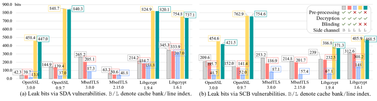
Figure 6: Leaked bits of RSA in different settings. Blinding for Libgcrypt 1.6.1 refers to RSA optimized with CRT (see Sec. 8.2.3). For cache line side channels (L in the last row of legend), we present detailed breakdown: enabling (✓ in the 4th row of legend) vs. disabling (✗ in the 4th row of legend) blinding, and with (✓ in the 2nd row) vs. w/o (✗ in the 2nd row) considering Pre-processing.

8.2.1 AES

Table 2: Leaked bits of AES/AES-NI in OpenSSL/MbedTLS.

	OpenSSL 3.0.0	OpenSSL 0.9.7	MbedTLS 3.0.0	MbedTLS 2.15.0
SCB	0	0	0	0
SDA	128.0	128.0	0	0

The side channels of AES collected from the in-house settings are deterministic. The SDA of AES standard T-table version can leak all key bits, but this implementation has no SCB [6, 57]. These facts serve as the ground truth for verifying CacheQL’s quantification and localization. MbedTLS by default uses AES-NI, which has no SDA/SCB. As shown in Table 2, CacheQL reports no leak in it.

CacheQL reports 128 bits SDA leakage in AES-128 of OpenSSL whereas the SCB leakage in this implementation is zero. This shows that the quantification of CacheQL is precise. We distribute the leaked bits to program points via Shapley value. All 128 bits are apportioned evenly toward 16 memory accesses in function _x86_64_AES_encrypt_compact. Manually, we find that these 16 memory accesses are all key-dependent table lookups.

8.2.2 Test Secure Implementations

CacheQL also examines secure cryptographic implementations with no leakage. For these cases, the quantification derived from CacheQL can also be seen as their correctness assessments. Given that said, as a dynamic method, CacheQL is for bug detection, not for verification.

ORAM. PathOHeap yields non-deterministic side channels, by randomly inserting dummy memory accesses to produce highly lengthy traces. Since it takes several hours to process one logged trace of RSA, we apply PathOHeap on AES from OpenSSL 3.0.0. Overall, PathOHeap delivers provable mitigation: memory access traces, after being processed by PathOHeap, should not depend on secrets. CacheQL  reports consistent and accurate findings to empirically verify PathOHeap, as the leaked bit is quantified as zero.

Constant-Time Implementations. 13 constant-time utilities [5] from Binsec/Rel [20] are evaluated using CacheQL. Side channel traces from these utilities are deterministic, whose quantified leaks are also zero. These results empirically show the correctness of CacheQL’s quantification.

8.2.3 RSA

RSA blinding is enabled by default in production cryptosystems. We quantify the information leakage of RSA with/without blinding, such that the logged traces are non-deterministic when blinding is on. As noted in Sec. 3 (), prior works mainly focus on the decryption fragment of RSA due to limited scalability [57, 22, 56, 6, 12]. As will be shown, this tradeoff neglects many vulnerabilities, primarily in the pre-processing modules of cryptographic libraries, e.g., key parsing and BIGNUM initialization. CacheQL efficiently analyzes the whole trace, covering Pre-processing and Decryption (see Fig. 6). As an ablation, CacheQL also analyzes only Decryption, e.g., the green bar in Fig. 6.

Setup. Libgcrypt 1.9.4 uses blinding on both ciphertext and private keys. We enable/disable them together. Libgcrypt 1.6.1 lacks blinding but implements the standard RSA and another version using Chinese Remainder Theorem (CRT). Libgcrypt 1.9.4 uses blinding in the CRT version and disables blinding in the standard one. We evaluate these two RSA versions in Libgcrypt 1.6.1. MbedTLS does not allow disabling blinding.

Results Overview. Fig. 6 shows the quantitative results. Since cache bank only discards two least significant bits of the memory addresses, it leaks more information than using cache line which discards six bits. Blinding in modern cryptosystems notably reduces leakage: blinding influences secret-dependent memory accesses, introducing non-determinism to prevent attackers from inferring secrets. Leakage varies across different software and variants of the same software. Secrets are leaked via SCB and SDA to varying degrees. If blinding is disabled, the total leak bits when considering only Decryption are close to the whole pipeline’s leakage. This is reasonable as they leak information from the same source. With blinding enabled, leakage in Decryption is inhibited, and Pre-processing contributes the most leakage. Though blinding minimizes leakage in Decryption, Pre-processing remains highly vulnerable, and it is generally overlooked previously.

OpenSSL. OpenSSL 3.0.0 has higher SCB leakage in Pre-processing with blinding enabled. As will be discussed in Sec. 8.3, this leakage is primarily introduced by BN_bin2bn and bn_expand2 functions, which convert key from string into BIGNUM. The issue persists with OpenSSL 0.9.7. Moreover, compared with ver. 3.0.0, OpenSSL 0.9.7 has more SDA (but less SCB) leakage with blinding enabled. These gaps are also primarily caused by the BN_bin2bn function in Pre-processing. We find that OpenSSL 3.0.0 skips leading zeros when converting key from string into BIGNUM, which introduces extra SCB leakage. In contrast, OpenSSL 0.9.7 first converts the key with leading zeros into BIGNUM and then uses bn_fix_top to remove those leading zeros, causing extra SDA leakage. Also, if blinding is disabled, OpenSSL 0.9.7 leaks approximately twice as many bits as OpenSSL 3.0.0. According to the localization results of CacheQL, OpenSSL 0.9.7 has memory accesses and branch conditions that directly depend on keys, which are vulnerable and lead to over 800 bits of leakage. We manually check OpenSSL 3.0.0 and find that most of those vulnerable functions have been re-implemented in a constant-time way.

MbedTLS. CacheQL finds many SDA in MbedTLS 3.0.0, which primarily occurs in the mbedtls_mpi_read_binary and mbedtls_mpi_copy functions during Pre-processing. The problem is not severe in ver. 2.15.0. We manually compare the two versions’ Pre-processing and find that the CRT initialization routines differ. In short, MbedTLS 3.0.0 avoids computing DP, DQ and QP (parts of the RSA private key in CRT) and instead reads them from the PKCS1 structure, and therefore, mbedtls_mpi_copy function is called for several times. The 2.15.0 version calculates DP, DQ and QP from the private key via BIGNUM involved functions (e.g., mbedtls_mpi_mul_mpi). The mbedtls_mpi_copy function leaks information via SDA and SCB, whereas the BIGNUM computation in the 2.15.0 version mainly leaks via SCB. This difference also explains why both versions have many SCB, which are dominated by their Pre-processing.

Libgcrypt. Libcrypt 1.9.4 has most SCB leakage in Pre-processing with blinding enabled. Nearly all leaked bits are from the do_vsexp_sscan function, which parses the key from s-expression. Decryption only leaks negligible bits. Manual studies show that in Libgcrypt 1.9.4, most BIGNUM-involved functions in Decryption are constant time and safe. Nevertheless, CacheQL identifies leaks in do_vsexp_sscan. This illustrates that CacheQL comprehensively analyzes production cryptosystems, whereas developers neglect patching all sensitive functions in a constant-time manner, enabling subtle leakages. Also, both versions have SDA leakage primarily in the _gcry_mpi_powm function; this is also noted in prior works [57, 56, 12]. As aforementioned, Libgcrypt 1.9.4 uses the standard RSA without CRT when blinding is disabled. The 1.6.1 version does not offer blinding for both the standard RSA and the CRT version. It’s obvious that the standard version leaks more than the CRT version.

Correctness. It is challenging to obtain ground truth in our evaluation. Aside from the AES cases and secure implementations in Sec. 8.2.2 who have the “ground truth” (either leaking 128 bits or zero bits) to compare with, there are several cases in RSA whose leaked bits can be calculated manually, facilitating to assess the correctness of CacheQL’s quantification.

$\text{Case}_{1}$: BN_num_bits_word function in OpenSSL 0.9.7, which is first identified by CacheD [57] and currently fixed in OpenSSL 3.0.0, has 256 different entries depending on secrets. It leaks $-\log\frac{1}{256}$ = $8.0$ bits, in case entries are accessed evenly (which should be true since key bits are generated independently and uniformly). CacheQL reports the leakage as $7.4$ bits, denoting a close quantification.

$\text{Case}_{2}$: do_vsexp_sscan function (see Fig. 7) in both versions of Libgcrypt has control branches depending on whether a secret is greater than 10. The SCB at L2 of Fig. 7, in theory, leaks $-\log\frac{1}{16}+\log\frac{1}{10}$ = $0.68$ bits of information, as the possible key values are reduced from 16 to 10 when L2 is executed. Similarly, the SCB at L4 leaks $-\log\frac{1}{16}+\log\frac{1}{6}$ = $1.42$ bits. When CacheQL analyzes one trace, it apportions around $1$ bit to each of the two records corresponding to the SCB at L2 and L4. We interpret that CacheQL  provides accurate quantification and apportionment for this case.

8.3 RQ2: Localizing Leakage Sites

This section reports the leakage program points localized in RSA by CacheQL using Shapley value. We report representative functions in Table 3. See [4] for detailed reports.

When blinding is enabled, CacheQL localizes all previously-found leak sites and hundreds of new ones.

Table 3: Representative vulnerable func. and their categories.

OpenSSL 3.0.0	Type	MbedTLS 3.0.0	Type	Libgcrypt 1.9.4	Type
bn_expand2	, ,	mbedtls_mpi _copy	, ,	mul_n_basecase	, ,
BN_bin2bn	,	mbedtls_mpi _read_binary	,	do_vsexp_sscan	,
BN_mod_exp _mont	,	mpi_montmul	, ,	_gcry_mpih_mul	, ,
	,				,

Clarification. Some leak sites localized by CacheQL are dependent, e.g., several memory accesses within a loop where only the loop condition depends on secrets. To clarify, CacheQL does not distinguish dependent/independent leak sites, because from the game theory perspective, those dependent leak sites (i.e., players) collaboratively contribute to the leakage (i.e., the game). Also, reporting all dependent/independent leak sites may be likely more desirable, as it paints the complete picture of the software attack surface. Overall, identifying independent leak sites is challenging, and to our best knowledge, prior works also do not consider this. This would be an interesting future work to explore. On the other hand, vulnerabilities identified by CacheQL are from hundreds of functions that are not reported by prior works, showing that the localized vulnerabilities spread across the entire codebase, whose fixing may take considerable effort.

8.3.1 Categorization of Vulnerabilities

We list all identified vulnerabilities in [4]. Nevertheless, given the large number of (newly) identified vulnerabilities, it is obviously infeasible to analyze each case in this paper. To ease the comparison with existing tools that feature localization, we categorize leak sites from different aspects. We first categorize the leak sites according to their locations in the codebase ( and ). We then use and to describe how secrets are propagated. Moreover, since leaking-leading-zeros is less considered by previous work, we specifically present such cases in .

Leaking secrets in Pre-processing: Leak sites belonging to occur when program parses the key and initializes relevant data structures like BIGNUM. Note that this stage is rarely assessed by previous static (trace-based) tools due to limited scalability; empirical results are given in Table 5.

Leaking secrets in Decryption: While is primarily analyzed by prior static tools, in practice, they have to trade precision for speed, omitting analysis of full implicit information flow ( in Table 1). Therefore, their findings related to compose only a small subset of CacheQL’s findings. Also, prior dynamic tools, including DATA and MicroWalk, are less capable of detecting . This is because blinding is applied at Decryption ( in Table 1). DATA likely neglects leak sites when blinding is enabled since it merely differentiates logged side channel traces with key fixed/varied. MicroWalk incorrectly regards data accesses/control branches influenced by blinding as vulnerable. Blinding can introduce a great number of records (see Table 4 for increased trace length), and MicroWalk fails to correctly analyze all these cases.

Leaking leading zeros: Besides CacheQL, findings belonging to were only partially reported by DATA. Particularly, given DATA is less applicable when facing blinding (noted in Sec. 3), it finds only in Pre-processing, where blinding is not enabled yet. Since CacheQL can precisely quantify ( in Table 1) and apportion () leaked bits, it is capable of identifying in Decryption; the same reason also holds for . At this step, we manually inspected prior static tools and found they only “taint” the content of a BIGNUM, which is an array, if BIGNUM stores secrets. The number of leading zeros, which has enabled exploitations (CVE-2018-0734 and CVE-2018-0735 [58]) and is typically stored in a separate variable (e.g., top in OpenSSL), is neglected.

Leaking secrets via explicit information flow: Most findings belonging to have been reported by existing static tools. CacheQL re-discovers all of them despite it’s dynamic. We attribute the success to CacheQL’s precise quantification, which recasts MI as CP (Sec. 4.3), and localization, where leaks are re-formulated as a cooperative game (Sec. 6).

Leaking secrets via implicit information flow: As discussed above, prior static tools are incapable of fully detecting . Also, many findings of CacheQL in overlap with that in . Since DATA cannot handle blinding well (blinding is extensively used in Decryption), only a small portion of were correctly identified by DATA. DATA also has the same issue to neglect CacheQL’s findings in .

In sum, static-/trace-based tools (CacheD, CacheS, Abacus) can detect $\cap$ but cannot identify $\cup$ $\cup$ . As noted in Sec. 3, MicroWalk cannot properly differ randomness induced by blinding vs. keys, and is inaccurate for the RSA case with blinding enabled. DATA pinpoints (accordingly include $\cap$ ) and is less applicable for . CacheQL, due to its precise quantification, localization, and scalability, can identify $\cup$ $\cup$ $\cup$ $\cup$ .

8.3.2 Characteristics of Leakage Sites

The leakage sites exist in all stages of cryptosystems. Below, we use case studies and the distribution of leaked bits to illustrate their characteristics. In short, the leaks start when parsing keys from files and initializing secret-related BIGNUM, and persist during the whole life cycle of RSA execution.

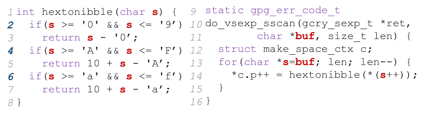
Figure 7: Simplified vulnerable program points localized in Libgcrypt 1.9.4. This function has SCB directly depending on bits of the key.

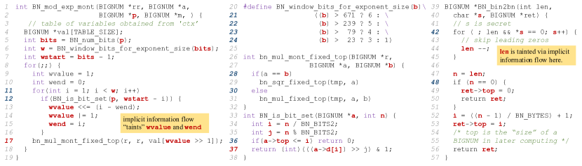
Figure 8: Vulnerable program points localized in OpenSSL 3.0.0. We mark the line numbers of SDA vulnerabilities and SCB vulnerabilities found by CacheQL. Secrets are propagated from p to other variables via explicit or implicit information flow, which confirm each SDA/SCB vulnerability found by CacheQL.

Case Study₁: Fig. 7 presents a case newly disclosed by CacheQL, which is the key parsing implemented in Libgcrypt 1.6.1 and 1.9.4. As discussed in Sec. 8.2.3 (see $\text{Case}_{2}$), this function has SCB explicitly depending on the key read from files. It therefore contains and . Similar leaks exist in other software. For instance, as localized by CacheQL and DATA, the EVP_DecodeUpdate function in two versions of OpenSSL have SDA via the lookup table data_ascii2bin when decoding keys read from files.

Case Study₂: Fig. 8 depicts the life-cycle of BIGNUM in OpenSSL 3.0.0, including initialization and computations. We show how secrets are leaked along the usage of BIGNUM.

1 BN_bin2bn@L39: A BIGNUM is initialized using s at L40, which is parsed from the key file in the .pem format. A for loop at L42 skips leading zeros, propagating s to len via implicit information flow. Then, len is propagated to top (L49 or L53). Thus, future usage of top clearly leaks secret.

2 BN_mod_exp_mont@L1: BN_num_bits is called to calculate #bits (after excluding leading zeros) of BIGNUM p. BN_num_bits further calls BN_num_bits_word which we have discussed in Sec. 8.2.3. #bits is stored in bits at L5. Later, bits is propagated to wstart at L7.

3 BN_window_bits_for_exponent_size@L20: w is propagated from bits at L6, given control branches from L21 to L24 directly depend on b.

4 BN_is_bit_set@L33: top of BIGNUM p directly decides the return value at L36. Its content, namely array d, also sets the return value at L37. Given wvalue and wend at L13 and L15 are updated according to the return value of BN_is_bit_set, they are thus implicitly propagated.

5 bn_mul_mont_fixed_top@L26: The access to array val at L17 is indexed with wvalue, and therefore, it induces SDA. Variable b at L27 is also propagated via wvalue, and the if branch at L28 thus introduces SCB.

Overall, 1 executes at Pre-processing and is only detected by DATA and CacheQL. It has both explicit (L47) and implicit (L42) information flow. Thus, it has    . Similarly, 2 contains    . Both 3 and 4 have   . 5 only has  . Among the leak sites discussed above, only five SCB at L21-L24 and L36 are detected by previous static tools; remaining ones are newly reported by CacheQL.

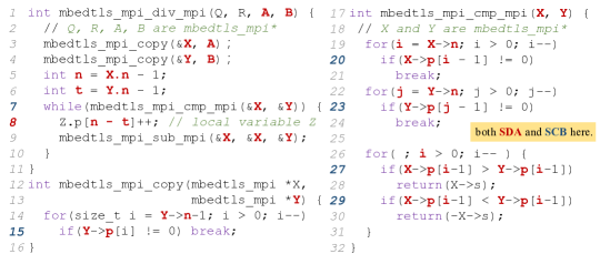
Figure 9: Vulnerable program points localized in MbedTLS 3.0.0. We mark the line numbers of SDA and SCB.

Case Study₃: Fig. 9 shows leaking sites disclosed by CacheQL in MbedTLS 3.0.0. In short, MbedTLS has similar implementation of BIGNUM with OpenSSL, where the variable n in BIGNUM stores the number of leading zeros. Later computations rely on n for optimization, for instance, the SDA at L8 in mbedtls_mpi_div_mpi@L1. It’s worth noting that mbedtls_mpi_copy@L12 is extensively called within the life cycles of all involved BIGNUM, contributing to notable leaks in the whole pipeline. Similar leaks also exist in MbedTLS 2.15.0. See our website [4] for more details.

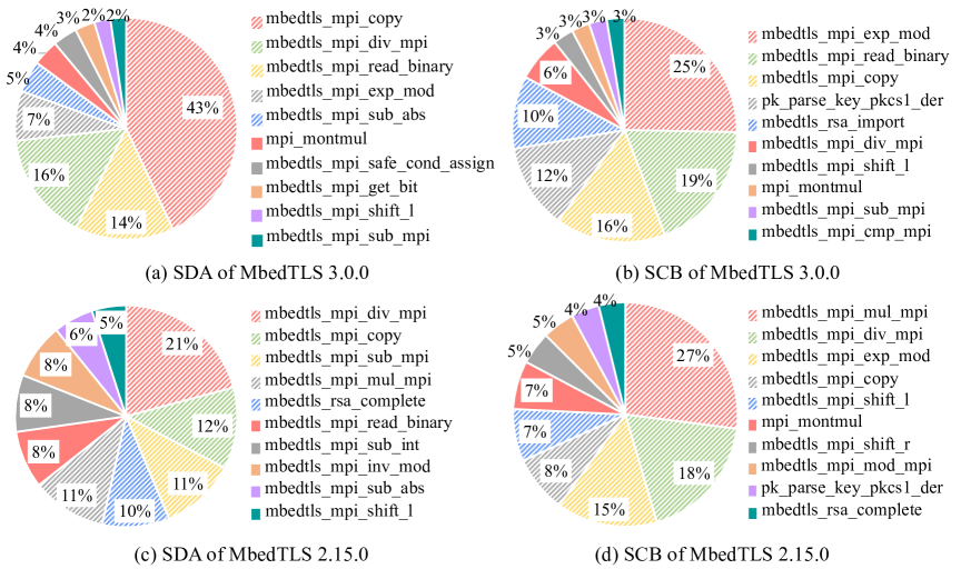
Figure 10: Distribution of top-10 functions in MbedTLS leaking most bits via either SDA or SCB vulnerabilities. Legend are in descending order.

Distribution. Fig. 10 reports the distribution of leaked bits among top-10 vulnerable functions localized in MbedTLS. The two versions of MbedTLS primarily leak bits in Pre-processing and have different strategies when initializing BIGNUMs for CRT optimization. Thus, the distributions of most vulnerable functions vary. For instance, the most vulnerable functions in ver. 2.15.0 are for multiplication and division; they are involved in calculating BIGNUMs for CRT. Notably, mbedtls_mpi_copy is among the top-5 vulnerable functions on all four charts in Fig. 10. This function leaks the leading zeros of the input BIGNUMs via both SDA and SCB. The mbedtls_mpi_copy function, as a memory copy routine function, is frequently called (e.g., more than 1,000 times in ver. 2.15.0). Though this function only leaks the leading zeros, given that its input can be the private key or key-dependent intermediate value, the accumulated leakage is substantial.

8.4 RQ3: Performance Comparison

To assess CacheQL’s optimizations and re-formulations, we compare CacheQL with previous tools on the speed, scalability, and capability of quantification and localization.

Table 4: Padded length of side channel traces collected using Intel Pin. The above/below five rows are for SDA/SCB.

	Pre-processing	-	Pre-processing	-
	Decryption	Decryption	Decryption	Decryption
	Blinding	Blinding	-	-
OpenSSL 3.0.0	$256\times 256\times 64$	$256\times 256\times 15$	$256\times 256\times 40$	$256\times 256\times 9$
OpenSSL 0.9.7	$256\times 256\times 20$	$256\times 256\times 14$	$256\times 256\times 14$	$256\times 256\times 13$
MbedTLS 3.0.0	$256\times 256\times 16$	$256\times 256\times 2$	N/A	N/A
MbedTLS 2.15.0	$256\times 256\times 14$	$256\times 256\times 2$	N/A	N/A
Libgcrypt 1.9.4	$256\times 256\times 36$	$256\times 256\times 22$	$256\times 256\times 26$	$256\times 256\times 25$
Libgcrypt 1.6.1	$256\times 256\times 5$	$128\times 128\times 19$	$256\times 256\times 11$	$256\times 256\times 10$
OpenSSL 3.0.0	$256\times 256\times 40$	$256\times 256\times 10$	$256\times 256\times 24$	$256\times 256\times 4$
OpenSSL 0.9.7	$256\times 256\times 8$	$256\times 256\times 5$	$256\times 256\times 5$	$256\times 256\times 4$
MbedTLS 3.0.0	$256\times 256\times 6$	$256\times 256\times 1$	N/A	N/A
MbedTLS 2.15.0	$256\times 256\times 6$	$256\times 256\times 1$	N//A	N/A
Libgcrypt 1.9.4	$256\times 256\times 12$	$256\times 256\times 8$	$256\times 256\times 10$	$256\times 256\times 9$
Libgcrypt 1.6.1	$256\times 256\times 3$	$128\times 128\times 8$	$256\times 256\times 6$	$256\times 256\times 5$

Trace Statistics. We report the lengths (after padding) of traces collected using Pin in Table 4. In short, all traces collected from real-world cryptosystems are lengthy, imposing high challenge for analysis. Nevertheless, CacheQL employs encoding module $\mathcal{S}$ and compressing module $\mathcal{R}$ to effectively process lengthy and sparse traces, as noted in Sec. 5.

Impact of Re-Formulations/Optimizations. CacheQL casts MI as CP when quantifying the leaks. This re-formulation is faster (see comparison below) and more precise, because calculating MI via MP (as done in MicroWalk) cannot distinguish blinding in traces. As reported in Table 4, a great number of records are related to blinding, and they lead to false positives of MicroWalk. For localization, the unoptimized Shapley value has $\mathcal{O}(2^{N})$ computing cost. Given the trace length $N$ is often extremely large (Table 4), computing Shapley value is infeasible. With our domain-specific optimizations, the cost is reduced as nearly constant.

8.4.1 Time Cost and Scalability

Table 5: Scalability comparison of static- or trace-based tools.

	CacheD	Abacus	CacheS	CacheAudit
Technique	symbolic execution		abstract interpretation
Libgcrypt	fail ($>$ 48h)	fail ($>$ 48h)	fail	fail
Libjpeg	fail	fail	fail	fail

Scalability Issue of Static-/Trace-Based Tools. As noted in in Sec. 3, prior static- or trace-based analyses rely on expensive and less scalable techniques. They, by default, primarily analyze a program/trace cut and neglect those pre-processing functions in cryptographic libraries. To faithfully assess their capabilities, we configure them to analyze the entire trace/software (which needs some tweaks on their codebase). We benchmark them on Libjpeg and RSA of Libgcrypt 1.9.4. Abacus/CacheD/CacheS/CacheAudit can only analyze 32-bit x86 executable. We thus compile 32-bit Libgcrypt and Libjpeg. Results are in Table 5. CacheS and CacheAudit throw exceptions of unhandled x86 instruction. Both tools, using rigorous albeit expensive abstraction interpretation, appear to handle a subset of x86 instructions. Fixing each unhandled instruction would presumably require defining a new abstract operator [19], which is challenging on our end. Abacus and CacheD can be configured to analyze the full trace of Libgcrypt. Nevertheless, both of them fail (in front of unhandled x86 instructions) after about 48h of processing. In contrast, CacheQL takes less than 17h to finish the training and analysis of the Libcrypt case; see Table 6.

Table 6: Training time of 50 epochs for the RSA cases.

	SDA				SCB
Configuration	Pre.	-	Pre.	-	Pre.	-	Pre.	-
	Dec.	Dec.	Dec.	Dec.	Dec.	Dec.	Dec.	Dec.
	Blind.	Blind.	-	-	Blind.	Blind.	-	-
OpenSSL 3.0.0	$22$h	$5$h	$3$h	$50$min	$13$h	$3$h	$2.5$h	$20$min
OpenSSL 0.9.7	$6.5$h	$5$h	$1$h	$1$h	$2.5$h	$1.5$h	$25$min	$20$min
MbedTLS 3.0.0	$5$h	$40$min	N/A	N/A	$2.5$h	$20$min	N/A	N/A
MbedTLS 2.15.0	$5$h	$40$min	N/A	N/A	$2.5$h	$20$min	N/A	N/A
Libgcrypt 1.9.4	$12.5$h	$7.5$h	$1.5$h	$1.5$h	$4$h	$2.5$h	$50$min	$45$min
Libgcrypt 1.6.1	$1.5$h	$1.5$h	$55$min	$50$min	$1$h	$40$min	$30$min	$25$min

• 1. Due to the limited space, we use Pre., Dec., and Blind. to denote Pre-processing, Decryption, and Blinding, respectively.

• 2. Blind. has $\times 4$ training samples.

Training/Analyzing Time of CacheQL. Table 6 presents the RSA case training time, which is calculated over 50 epochs (the maximal epochs required) on one Nvidia GeForce RTX 2080 GPU. In practice, most cases can finish in less than 50 epochs. For AES-128, training 50 epochs takes about 2 mins. Training 50 epochs for Libjpeg/PathOHeap takes 2-3 hours. As discussed in Sec. 4.3, since we transform computing MI as estimating CP, CacheQL only needs to be trained (for estimating CP) once. Once trained, it can analyze 256 traces in 1-2 seconds on one Nvidia GeForce RTX 2080 GPU, and less than 20 seconds on Intel Xeon CPU E5-2683 of 4 cores.

In sum, CacheQL is much faster than existing trace-based/static tools. By using CP, it principally reduces computing cost comparing with conventional dynamic tools (see Sec. 4). We also note that it is hard to make a fully fair comparison: training CacheQL can use GPU while existing tools only support to use CPUs. Though CacheQL has smaller time cost on the GPU (Nvidia 2080 is not very powerful), we do not claim CacheQL is faster than prior dynamic tools. In contrast, we only aim to justify that CacheQL is not as heavyweight as audiences may expect. Enabled by our theoretical and implementation-wise optimizations, CacheQL efficiently analyzes complex production software.

8.4.2 Capability of Quantification and Localization

Small Programs and Trace cuts. As evaluated in Sec. 8.4.1, previous static-/trace-based tools are incapable of analyzing the full side channel traces. Therefore, we compare them with CacheQL using small program (e.g., AES) and trace cuts.

Overall, the speed of CacheQL (i.e., training + analyzing) still largely outperforms static/trace-based methods. For instance, CacheD [57], a qualitative tool using symbolic execution, takes about 3.2 hours to analyze only the decryption routine of RSA in Libgcrypt 1.6.1 without considering blinding. CacheQL takes under one hour for this setting. In addition, Abacus [6], which performs quantitative analysis with symbolic execution, requires 109 hours to process one trace of Libgcrypt 1.8. Note that it only analyzes the decryption module (several caller/callee functions) without considering the blinding, pre-rocessing functions, etc. In contrast, CacheQL can finish the training within 2 hours (the trace length of Libgcrypt 1.9 is about the same as ver. 1.8) in this setting. It’s worth noting that, CacheQL only needs to be trained for once, and it takes only several seconds to analyze one trace. That is, when analyzing multiple traces, previous tools has fold increase on the time cost whereas CacheQL only adds several seconds.

The quantification/localization precision of CacheQL is also much higher. Abacus reports 413.6 bits of leakage for AES-128 (it neglects dependency among leakage sites, such that the same secret bits can be repetitively counted at different leakage sites), which is an overestimation since the key has only 128 bits. For RSA trace cuts, Abacus under-quantifies the leaked bits because it misses many vulnerabilities due to implicit information-flow. When localizing vulnerabilities in AES-128, we note that all static/trace-based have correct results. For localization results of RSA trace cuts, see Sec. 8.3.1. In short, none of the previous tools can identify all the categories of vulnerabilities.

Dynamic Tools. Previous dynamic tools do not suffer from the scalability issue and have comparable speed with CacheQL. Nevertheless, they require re-launching their whole pipeline (e.g., sampling + analyzing) for each trace.

For quantification, MicroWalk over-quantifies the leaked bits of RSA as 1024 when blinding is enabled, since it regards random records as vulnerable. Similarly, it reports that ORAM cases have all bits leaked despite they are indeed secure. MicroWalk can correctly quantify the leaks of whole traces for AES cases and constant-time implementations, because no randomness exists. Nevertheless, since the same key bits are repeatedly reused on the trace, its quantification results for single record, when summed up, are incorrectly inconsistent with the result of whole trace. For localization, as summarized in Sec. 8.3.1, previous dynamic tools are also either incapable of identifying all categories of vulnerabilities or yields many false positive. For instance, MicroWalk can regards all records related to blinding (over 1M in OpenSSL 3.0.0; see trace statistics in Table 4) as “vulnerable”.

9 Discussion

Handling Real-World Attack Logs. Side channel observations (e.g., obtained in cross-virtual machine attacks [70]), are typically noisy. CacheQL handles real attack logs by considering noise as non-determinism (see Sec. 4.4), thus quantifying leaked bits in those logs. Nevertheless, we do not recommend localizing vulnerabilities using real attack logs, since mapping these records back to program statements are challenging. Pin is sufficient for developers to “debug”.

Analyzing Media Data. CacheQL can smoothly quantify and localize information leaks for media software. Unlike previous static-/trace-based tools, which require re-implementing the pipeline to model floating-point instructions for symbolic execution or abstract interpretation, CacheQL only needs the compressor $\mathcal{R}$ to be changed. In addition, CacheQL is based on NN, which facilitates extracting “contents” of media data to quantify leaks, rather than simply comparing data byte differences. See evaluation results in Appx. B.

Program Taking Public Inputs. We deem that different public inputs should not largely influence our analysis over cryptographic and media libraries, whose reasons are two-fold. First, for cryptosystems like OpenSSL, the public inputs (i.e., plaintext or ciphertext) has a relatively minor impact on the program execution flow. To our observation, public input values only influence a few loop iterations and if conditions. Media libraries mainly process private user inputs, which has no “public inputs”. In practice, the influences of public inputs (including other non-secret local variables) are treated as non-determinism by CacheQL. That is, they are handled consistently as how CacheQL  handles cryptographic blinding (Sec. 4.4), because neither is related to secret.

Given that said, configurations (e.g., cryptographic algorithm or image compression mode) may notably change the execution and the logged execution traces. We view that as an orthogonal factor. Moreover, modes of cryptographic algorithms and media processing procedures are limited. Users of CacheQL are suggested to fix the mode before launching an analysis with CacheQL, then use another mode, and so on.

Keystroke Templating Attacks. Quantifying and localizing the information leaks that enable keystroke templating attacks should be feasible to explore. With side channel traces logged by Intel Pin, machine learning is used to predict the user’s key press [55]. Given sufficient data logged in this scenario, CacheQL can be directly applied to quantify the leaked information and localize leakage sites.

Large Software Monoliths. For analyzing complex software like browsers and office products, our experience is that using Intel Pin to perform dynamic instrumentation for production browsers is difficult. With this regard, we anticipate adopting other dynamic instrumentors, if possible, to enable localizing leaks in these software. With correctly logged execution trace, CacheQL can quantify the leaked bits and attribute the bits to side channel records.

Training Dataset Generalization. One may question to what degree traces obtained from one program can be used as training set for detecting leaks in another. In our current setup, we do not advocate such a “transfer” setting. Holistically, CacheQL learns to compute PD by accurately distinguishing traces produced when the software is processing different secret inputs. By learning such distinguishability, CacheQL eliminates the need for users to label the leakage bits of each training data sample. Nevertheless, knowledge learned for distinguishability may differ between programs. It is intriguing to explore training a “general” model that can quantify different side channel logs, particularly when collecting traces for the target program is costly. To do so, we expect to incorporate advanced training techniques (such as transfer learning [46]) into our pipeline.

Key Generation. In RSA evaluations, we feed cryptographic libraries with the key in a file. That is, the cryptographic library execution does not involve “key generation”, which is not due to “limited coverage” of CacheQL. Previous works [44] have exploited RSA key generation. With manual effort, we find that the key generation functions heavily use BIGNUM, involving vulnerable BIGNUM initialization and computation functions already localized by CacheQL in Sec. 8.3, e.g., BN_bin2bn in Fig. 8 and BN_sub (see our full report [4]).

BIGNUM Implementation. We also investigate other cryptosystems. LibreSSL and BoringSSL are built on OpenSSL. Their BIGNUM implementations and OpenSSL share similar vulnerable coding patterns (i.e., the leading zero leak patterns; see of Sec. 8.3). We also find similar BIGNUM vulnerable patterns in Botan (see [1]). In contrast, we find Intel IPP does not use an individual variable to record #leading zeros in BIGNUM (see [2]), hence it is likely free of .

10 Conclusion

We present CacheQL to quantify cache side channel leakages via MI. We also formulate secret leak as a cooperative game and enable localization via Shapley value. Our evaluation shows that CacheQL overcomes typical hurdles (e.g., scalability, accuracy) of prior works, and computes information leaks in real-world cryptographic and media software.

Appendix A Libjpeg and Prime+Probe Evaluation

Data Preparing. We choose the CelebA dataset [40] as the image inputs of Libjpeg. The CelebA consists of 160,000 training and 10,000 validation images. We use the training images and their corresponding side channel traces to estimate CP via $\mathcal{F}_{\theta}$. The validation images and their induced side channels are adopted for de-biasing (in case there exists non-determinism).

Trace Logging. Following the same configuration of Sec. 8, we use Pin to log execution traces of Libjpeg.

Logging via Prime+Probe. Besides using Pin, we collect cache set access traces (for both cryptosystems and Libjpeg) via Prime+Probe [53], in userspace-only scenarios. Following [66], we use Mastik [63], a micro-architectural side channel toolkit, to perform Prime+Probe and log victim’s access toward L1D and L1I cache. We use Linux taskset to pin victim software and the spy process on the same CPU core. Scripts of Prime+Probe experiments are at [4].

A.1 Libjpeg

Quantification. Libjpeg does not contain mitigations like blinding. Thus, side channels collected by Pin are deterministic. Nevertheless, we argue that merely considering the difference among SDA/SCB, which is a conventional setup for cryptosystems, will over-estimate the leakage. The reasons are two-fold: 1) Traces can be largely divergent by tweaking trivial pixels in the input images, e.g., background color pixels. 2) Even if all pixels are equally sensitive, the leakage may be insufficient to recover input images. For instance, attackers only infer whether each pixel value is larger than a threshold (as how keys are usually recovered) and obtain a binary image — it’s still infeasible to recognize humans in such images.

To handle these, we extend the generalizability consideration, which is proposed to handle non-deterministic side channels derived from cryptosystems, to quantify deterministic side channels made by Libjpeg. Therefore, our quantification is the same as for processing non-deterministic side channels of cryptosystems. Due to the aforementioned issue, we deem trivial pixels contain little information. As introduced in Sec. 4.4, CacheQL  should accordingly report a zero leakage since these non-sensitive factors are not generalizable.

Given that the #images is infinite, it’s infeasible to decide the value of $p(F)/p(T)$ in Eq. 3 which should be a constant. We thus report the leakage ratio for Libjpeg. As shown in Table 7, leakage ratios reach 100% for SDA and SCB if we only consider the distinguishability, which indicates side channels can differ images. Nevertheless, the leakage ratios are reduced to 93% for SDA and 49% for SCB when we faithfully take generalizability into account. To further prove that CacheQL indeed captures the critical information in face photos, we present the output of $\mathcal{R}$ in Fig. 11. The output manifests common human face features like eyes and noses.

Table 7: Leakage ratios (see Eq. 4) of Libjpeg without $\rightarrow$ with considering generalizability.

	SDA	SCB
cache line	100% $\rightarrow$ 93%	100% $\rightarrow$ 49%

Table 8: Representative vulnerable functions localized in Libjpeg and their types.

Function	Type
decode_mcu	SDA, SCB
jsimd_ycc_extbgrx_convert_avx2	SDA
jsimd_idct_islow_avx2	SDA, SCB

Localization. Representative vulnerable functions of Libjpeg are given in Table 8. The leaked bits are spread across hundreds of program points, mostly from the IDCT, YCC encoding, and MCU modules. Libjpeg converts JPEG images into bitmaps, whose procedure has many SDA and SCB. We manually checked our findings, which are aligned with [66]. Nevertheless, the YCC encoding-related functions are newly found by us. CacheQL  also shows that SDA in IDCT leaks the most bits, whereas the MCU modules leak more bits via SCB. [66] flags those issues without quantification.

Table 9: Leaks of side channels collected via Prime+Probe.

	RSA D	RSA D	RSA D	RSA D
#Repeating	1	2	4	8
Leakage	19.3 (1.8%)	29.4 (2.8%)	34.9 (3.4%)	35.5 (3.4%)
	RSA D	RSA I	Libjpeg D	Libjpeg I
#Repeating	16	8	8	8
Leakage	35.6 (3.4%)	21.6 (2.1%)	20.8%	12.9%

• 1. “D” denotes L1 D cache whereas “I” denotes L1 I cache.

• 2. We also report leakage ratios for RSA cases to ease comparison.

A.2 Prime+Probe

Following previous setups [66], a common Prime+Probe is launched on the same core with the victim software and periodically probes L1 cache when the victim software is executed. This mimics a practical and powerful attacker and is also the default setup of the Prime+Probe toolkit [63] leveraged in our evaluation and relevant research in this field. To prepare traces about Pre-processing, we halt the victim program after the pre-processing stage. Generally, launching Prime+Probe is costly. Without loss of generality, we use Prime+Probe to collect RSA side channels from OpenSSL 0.9.7 and Libjpeg. Attackers often repeat launching Prime+Probe [70]. As in Table 9, repeating an attack to collect more logs does improve information, but only marginal. Compared to merely doing Prime+Probe once, repeating $\times$4 yields more information. However, repeating more times does not necessarily improve, since the information source is always the same. We also note that Pre-processing has more leaks: for two (RSA, #Repeating=8) cases of L1 D and I cache (i.e., the 2nd and 3rd columns in the last row), Pre-processing has 22.5 (total 35.5) and 14.1 (total 21.6) leaked bits.

Libjpeg leaks more information than RSA. Not like recovering keys where each key bit needs to be analyzed, recovering every pixel is not necessary for inferring images. As previously stated [66], pixels conform to specific constraints to form meaningful contents (e.g., a human face), which typically have lower dimensions than pixel values. As a result, extracting these constraints can give rich information already.

Appendix B Transformations in $\mathcal{R}$

As stated in Sec. 5, we adopt different mathematical transformations in $\mathcal{R}$ for media data and cryptographic keys. In what follows, we elaborate on compressing latent vectors of media data and secret keys with different transformations in $\mathcal{R}$.

Media Data. We use image to demonstrate the cases for media data; the conclusion can be extended to other media data straightforward [66]. It is generally obscure to measure the amount of information encoded in high-dimensional media data like images [68]. To extract information, an image, before being fed into modern neural networks (e.g., classifier $\mathcal{C}$ in CacheQL), is generally normalized into $[-1,1]$ and represented as a $channel\times width\times height$ matrix [33]. Let a private image be $k_{m}$ and the associated side channel log be $o_{m}$, we set the output of $\mathcal{S}(o_{m})$ as a matrix of the same size. Accordingly, our compressor $\mathcal{R}_{m}$ is implemented using the $tanh:[-\infty,\infty]\rightarrow[-1,1]$ function, facilitating $H(o_{m})\leq H(k_{m})$. $tanh$ is parameter free (i.e., $\theta_{\mathcal{R}}=\emptyset$), eliminating extra training cost. Also, if certain properties in an image are particularly desirable by attackers, e.g., the gender of portrait images, $k_{m}$ and the matrix from $\mathcal{S}(o_{m})$ can be replaced with a vectorized representation for image properties. We refer readers to [47] for vectorizing image attributes.

Cryptographic Keys. For a cryptographic key $k_{c}$ of length $L$, there are total $2^{L}$ uniformly distributed key instances. The information in one key instance is thus $H(k)=\log 2^{L}=L$ bits. Since a key only contains binary values and neural networks are hard to be deployed with binary parameters, for the associated side channel log $o_{c}$, we need to transform the floating-point encoding output $\mathcal{S}(o_{c})$, which is accordingly a vector of length $L$, into binary bits. Existing profiling-based side channel attacks map side channels to keys via $L$ bit-wise classification tasks  [30, 32, 27]. In each task, a floating point is transformed to 1 if it is greater than a threshold. Nevertheless, this transformation is not applicable in $\mathcal{R}$, given that it is not differentiable, which impedes the optimization of $\theta$. Inspired by the optimization for binary variables  [17, 18], we design $\mathcal{R}_{c}$ by joining two components: 1) a non-parametric $sigmoid:[-\infty,\infty]\rightarrow[0,1]$ function which generates $L$ independent (as bits in $k_{c}$ are independent) probabilities, and 2) a parametric Bernoulli distribution $Bern:\Pr(Bern(\cdot)=1)+\Pr(Bern(\cdot)=0)=1$ which takes its inputs, i.e., $sigmoid(\mathcal{S}(o_{c}))$, as parameters for optimization. Thus, we have $\mathcal{R}_{c}=Bern\circ sigmoid$ and $\theta_{\mathcal{R}_{c}}=sigmoid(\mathcal{S}(o_{c}))$. See our codebase [4] for details.

Recall as we discussed in Sec. 5, $\mathcal{R}$ is designed for shrinking maximal information in a side channel trace $o$, enabled by this principle, CacheQL is “forced” to focus on secret-related information. Outputs of $\mathcal{R}$ are shown in Fig. 11: it captures common facial features, such as eyes and mouth, when quantifying information leaks for human photos.

Figure 11: Outputs of $\mathcal{R}$ when quantifying leakage of images.

Appendix C Reconstruct Secrets From Side Channels

Appx. B demonstrates that $\mathcal{R}$ captures facial attributes when quantifying leakage of portrait photos. Readers may question whether CacheQL  can directly reconstruct secrets from side channels. To this end, we extend CacheQL by tweaking the optimization objectives (only adds one line of code; see our manuals [4]), and present results in Table 10. We show reconstructed images on our website [4]. Overall, keys/images with reasonable quality are reconstructed using traces logged by Intel Pin or Prime+Probe. In particular, reconstructed images have more vivid appearance than Fig. 11; it’s reasonable since quantifying leaks emphasizes on the distinguishability. These promising results illustrate the superiority of CacheQL’s design and extendability, and the exploitability of localized program points. Having stated that, we clarify that aligned with prior works in this field, CacheQL is a bug detector, not for reconstructing secret in real attacks. Also, as a proof of concept, the extended CacheQL shows the feasibility of key/image reconstruction; the quality of reconstructed keys/images may be further improved [66], which we leave as one future work.

Table 10: Quantitative evaluation of the reconstruction.

	∗Libjpeg (Pin)	†OpenSSL 0.9.7 (Pin)	∗Libjpeg (Prime+Probe)
DA/D cache	41.5%	58.2%	36.8%
CB/I cache	40.4%	57.7%	36.0%

• * We report percentage of reconstructed photos that are recognized as the same faces with the reference photos. We use the criterion of [66].

• $\dagger$ Pre-processing + Decryption with blinding enabled. We report percentage of correct bits. Random guess (baseline) should be 50%.

Appendix D Extended Proof of Eq. 10

This Appendix section proves Eq. 10 in a two-step approach; we refer the following proof skeleton to [8, 54]. Since $c(k,o)$ is only decided by $\mathcal{F}_{\theta}$, for simplicity, we also denote it as a parameterized function. In particular, Lemma 1 first shows that the empirically measured $\hat{I}^{(n)}_{\theta^{\dagger}}(K;O)$ is consistent with $\hat{I}_{\theta^{\dagger}}(K;O)$. Lemma 2 then proves that $\hat{I}_{\theta^{\dagger}}(K;O)$ stays close to $I(K;O)$. In all, Tsai et al. [54] has pointed out that the following two prepositions hold for neural networks:

Proposition 1 (Boundness).

$\forall\hat{c}_{\theta}$ and $\forall k,o$, there exist two constant bounds $B_{l}$ and $B_{u}$ such that $B_{l}\leq\log\hat{c}_{\theta}(k,o)\leq B_{u}$.

Proposition 2 ($\log$-smoothness).

$\forall k,o$ and $\forall\theta_{1},\theta_{2}\in\Theta$, $\exists\alpha>0$ such that $|\log\hat{c}_{\theta_{1}}(k,o)-\log\hat{c}_{\theta_{2}}(k,o)|\leq\alpha\|\theta_{1}-\theta_{2}\|$.

Proposition 1 states that outputs of a neural network are bounded and Proposition 2 clarifies that the output of a neural network will not change too much if the parameter $\theta$ change slightly [54]. By incorporating the bounded rate of uniform convergence on parameterized functions [7], we have:

Lemma 1 (Estimation).

$\forall\epsilon>0$,

$$\Pr\limits_{\{\langle k,o\rangle\}^{(n)}}\left(\sup\limits_{\hat{c}_{\theta^{\dagger}}\in\mathcal{C}}\left|\hat{I}_{\theta^{\dagger}}^{(n)}(K;O)-\mathbb{E}_{P_{K\times O}}[\log\hat{c}_{\theta^{\dagger}}(k,o)]\right|\geq\epsilon\right)$$

$$\leq 2|\Theta|\exp\left(\frac{-n\epsilon^{2}}{2(B_{u}-B_{l})^{2}}\right).$$

Lemma 1 applies the classical consistency theorem [23] for extremum estimators. Here, extremum estimators denote parametric functions optimized via maximizing or minimizing certain objectives; note that $\hat{c}_{\theta}$ is optimized to maximize the binary cross-entropy in Eq. 6. It illustrates that $\hat{I}^{(n)}_{\theta^{\dagger}}(K;O)$ convergent to $\hat{I}_{\theta^{\dagger}}(K;O)$ as $n$ grows. Future, based the universal approximation theory of neural networks [29], we have:

Lemma 2 (Approximation).

$\forall\epsilon>0$, there exists a family of neural networks $N=\{\hat{c}_{\theta}:\theta\in\Theta\}$ such that

$$\inf\limits_{\hat{c}_{\theta}\in N}|\mathbb{E}_{P_{K\times O}}[\log\hat{c}_{\theta}(k,o)]-I(K,O)|\leq\epsilon.$$

Lemma 2 states that $\hat{I}_{\theta^{\dagger}}(K;O)$ can approximate $I(K;O)$ with arbitrary accuracy. Therefore, Eq. 10 can be derived from Lemma 1 and Lemma 2 based on the triangular inequality.

Appendix E Key Properties of Shapley Values

Following Sec. 6, this Appendix shows several key properties of Shapley value. We discuss why it is suitable for side channel analysis and how the properties help our localization. To clarify, the following theorems are not proposed by this paper; they are for reader’s reference only.

Theorem 1 (Efficiency [49]).

The sum of Shapley value of all participants (i.e., side channel records) equals to the value of the grand coalition:

$$\sum_{i\in R^{o}}\pi_{i}(\phi)=\phi(o)-\phi(o_{\emptyset}).$$ (13)

Theorem 1 states that the assigned Shapley value for each side channel record satisfies the apportionment defined in Definition 1. $\phi(o_{\emptyset})=0$ since an empty $o$ leaks no secret.

Theorem 2 (Symmetry [49]).

If $\forall S\subseteq R^{o}\setminus\{i,j\}$, $i$- and $j$-th players are equivalent, i.e., $\phi(o_{S\cup\{i\}})=\phi(o_{S\cup\{j\}})$, then $\pi_{i}(\phi)=\pi_{j}(\phi)$.

Theorem 2 states records in $o$ contributing equally to leakage have the same Shapley value. Divergent Shapley values suggest divergent leakage on the relevant program points. It ensures that all contributions are awarded Shapley values.

Theorem 3 (Dummy Player [49]).

If the $i$-th participant is a dummy player, i.e., $\forall S\subseteq R^{o}\setminus\{i\},\phi(o_{S\cup\{i\}})-\phi(o_{S})=\phi(o_{\{i\}})-\phi(o_{\emptyset})$, then $\pi_{i}(\phi)=\phi(o_{\{i\}})-\phi(o_{\emptyset})$.

Theorem 3, dubbed as “Dummy Player,” states that the information leakage in one program point is not distributed to non-correlated points. In sum, Theorem 2 and Theorem 3 guarantee that the Shapley value apportionment is accurate. Further, if $\phi(o_{\{i\}})=\phi(o_{\emptyset})$, we have the following theorem.

Theorem 3.1 (Null player [49]).

If the $i$-th participant has no contribution to any grand coalition game $\phi$, i.e., $\forall S\subseteq R^{o}\setminus\{i\},\phi(o_{S\cup\{i\}})=\phi(o_{S})$, then $\pi_{i}(\phi)=0$.

Theorem 3.1 is one special case of Theorem 3, and it guarantees that the Shapley value has no false negative. That is, program points assigned with a zero Shapley value is guaranteed to not contribute to information leakage.

Theorem 4 (Linearity [49]).

If two coalition games, namely $\phi$ and $\psi$, are combined, then $\pi_{i}(\phi+\psi)=\pi_{i}(\phi)+\pi_{i}(\psi)$ for $\forall i\in R^{o}$.

Theorem 4 implies that if a secret has several independent components, then the assigned Shapley value for each side channel record equals to the linear sum of secrets leaked on this record from all components. For instance, let $\pi(\phi_{g})$ and $\pi(\phi_{a})$ be the leaked information by recovering two privacy-related properties, “gender” and “age,” over portrait photos. Since these two properties are independent, when considering both, the newly-computed leakage $\pi(\phi)$ must equal the sum of $\pi(\phi_{g})$ and $\pi(\phi_{a})$ according to Theorem 4. While this property allows for fine-grained leakage analysis, we currently do not separate a secret into independent components. We view this exploration as one future work.

Theorem 5 (Uniqueness [49]).

The apportionment derived from Shapley value is the only one that simultaneously satisfies Theorem 1, Theorem 2, Theorem 3 & 3.1, and Theorem 4.

Appendix F Responsible Disclosure

Table 11: Statistics of reported vulnerabilities.

	Reported flaws	Answered	Acknowledged flaws
OpenSSL	10 (functions)	10	10
MbedTLS	62 (leakage sites)	62	62
Libgcrypt	5 (functions)	0	0
Libjpeg	2 (functions)	2	2

We have reported our findings to developers. Since we find many vulnerabilities in each cryptosystems and media software (see a complete list at [4]), we summarize representative cases and also clarify the leakage to developers to seek prompt confirmation. Sometimes, as required, we further annotate the vulnerable statements (e.g., for MbedTLS developers). Table 11 lists the exact numbers of vulnerable functions/program points we reported.

By the time of writing, OpenSSL developers have confirmed BIGNUM related findings. MbedTLS developers also positively responded to our reports. We are discussing with them the disclosure procedure. Libjpeg developers agreed with our reported SDA/SCB cases but required PoC exploitations and patches to assess cost vs. benefit. We did not receive response from Libgcrypt developers.

References

- [1] Bignum implementation in botan. https://github.com/randombit/botan/blob/3.0.0-alpha1/src/lib/math/bigint/bigint.cpp#L210.
- [2] Bignum implementation in intel ipp. https://www.intel.com/content/www/us/en/develop/documentation/ipp-crypto-reference/top/appendix-a-support-functions-and-classes/classes-and-functions-used-in-examples/bignumber-class.html.
- [3] Openssl security policy. https://www.openssl.org/policies/secpolicy.html.
- [4] Research artifact. https://github.com/Yuanyuan-Yuan/CacheQL.
- [5] Test cases from binsec/rel. https://github.com/binsec/rel_bench/tree/82b9ad267a8a86c2cfd8560755aa0d9a0ef5a627/src/ct/openssl_utility.
- [6] Qinkun Bao, Zihao Wang, Xiaoting Li, James R Larus, and Dinghao Wu. Abacus: Precise side-channel analysis. ICSE, 2021.
- [7] Peter L Bartlett. The sample complexity of pattern classification with neural networks: the size of the weights is more important than the size of the network. IEEE transactions on Information Theory, 44(2), 1998.
- [8] Mohamed Ishmael Belghazi, Aristide Baratin, Sai Rajeshwar, Sherjil Ozair, Yoshua Bengio, Aaron Courville, and Devon Hjelm. Mutual information neural estimation. ICML, 2018.
- [9] Fabrice Bellard. Qemu, a fast and portable dynamic translator. In USENIX annual technical conference, FREENIX Track, volume 41, pages 10–5555. Califor-nia, USA, 2005.
- [10] Richard Bellman. Dynamic programming. Science, 153(3731), 1966.
- [11] Yoshua Bengio, Aaron Courville, and Pascal Vincent. Representation learning: A review and new perspectives. TPAMI, 2013.
- [12] Robert Brotzman, Shen Liu, Danfeng Zhang, Gang Tan, and Mahmut Kandemir. CaSym: Cache aware symbolic execution for side channel detection and mitigation. In IEEE SP, 2018.
- [13] Javier Castro, Daniel Gómez, Elisenda Molina, and Juan Tejada. Improving polynomial estimation of the shapley value by stratified random sampling with optimum allocation. Computers & Operations Research, 82:180–188, 2017.
- [14] Javier Castro, Daniel Gómez, and Juan Tejada. Polynomial calculation of the shapley value based on sampling. Computers & Operations Research, 2009.
- [15] Sudipta Chattopadhyay, Moritz Beck, Ahmed Rezine, and Andreas Zeller. Quantifying information leakage in cache attacks via symbolic execution. TECS, 2019.
- [16] Duc-Hiep Chu, Joxan Jaffar, and Rasool Maghareh. Precise cache timing analysis via symbolic execution. RTAS, pages 1–12, 2016.
- [17] Matthieu Courbariaux, Yoshua Bengio, and Jean-Pierre David. Binaryconnect: Training deep neural networks with binary weights during propagations. In NIPS, 2015.
- [18] Matthieu Courbariaux, Itay Hubara, Daniel Soudry, Ran El-Yaniv, and Yoshua Bengio. Binarized neural networks: Training deep neural networks with weights and activations constrained to+ 1 or-1. arXiv preprint arXiv:1602.02830, 2016.
- [19] Patrick Cousot and Radhia Cousot. Abstract interpretation: a unified lattice model for static analysis of programs by construction of fixpoints. POPL, 1977.
- [20] Lesly-Ann Daniel, Sébastien Bardin, and Tamara Rezk. Binsec/rel: Efficient relational symbolic execution for constant-time at binary-level. IEEE S&P, 2020.
- [21] Goran Doychev, Dominik Feld, Boris Kopf, Laurent Mauborgne, and Jan Reineke. CacheAudit: A tool for the static analysis of cache side channels. In USENIX Sec., 2013.
- [22] Goran Doychev and Boris Köpf. Rigorous analysis of software countermeasures against cache attacks. PLDI, 2017.
- [23] Sara A Geer, Sara van de Geer, and D Williams. Empirical Processes in M-estimation. 2000.
- [24] Benedikt Gierlichs, Lejla Batina, Pim Tuyls, and Bart Preneel. Mutual information analysis, a generic side-channel distinguisher. In CHES’08, 2008.
- [25] Oded Goldreich and Rafail Ostrovsky. Software protection and simulation on oblivious rams. JACM, 1996.
- [26] Marcus Hähnel, Weidong Cui, and Marcus Peinado. High-resolution side channels for untrusted operating systems. USENIX ATC, 2017.
- [27] Benjamin Hettwer, Stefan Gehrer, and Tim Güneysu. Profiled power analysis attacks using convolutional neural networks with domain knowledge. SAC, 2018.
- [28] Geoffrey E Hinton and Richard S Zemel. Autoencoders, minimum description length, and helmholtz free energy. NIPS, 1994.
- [29] Kurt Hornik, Maxwell Stinchcombe, and Halbert White. Multilayer feedforward networks are universal approximators. Neural networks, 2(5):359–366, 1989.
- [30] Gabriel Hospodar, Benedikt Gierlichs, Elke De Mulder, Ingrid Verbauwhede, and Joos Vandewalle. Machine learning in side-channel analysis: a first study. Journal of Cryptographic Engineering, 2011.
- [31] Jan Jancar, Marcel Fourné, Daniel De Almeida Braga, Mohamed Sabt, Peter Schwabe, Gilles Barthe, Pierre-Alain Fouque, and Yasemin Acar. “they’re not that hard to mitigate”: What cryptographic library developers think about timing attacks. IEEE S&P, 2021.
- [32] Jaehun Kim, Stjepan Picek, Annelie Heuser, Shivam Bhasin, and Alan Hanjalic. Make some noise. unleashing the power of convolutional neural networks for profiled side-channel analysis. TCHES, 2019.
- [33] Alex Krizhevsky, Ilya Sutskever, and Geoffrey E Hinton. ImageNet classification with deep convolutional neural networks. NIPS, 2012.
- [34] Donggeun Kwon, HeeSeok Kim, and Seokhie Hong. Improving non-profiled side-channel attacks using autoencoder based preprocessing. IACR Cryptol., 2020.
- [35] Xianfeng Li, Tulika Mitra, and Abhik Roychoudhury. Accurate timing analysis by modeling caches, speculation and their interaction. DAC, 2003.
- [36] Yan Li, Vivy Suhendra, Yun Liang, Tulika Mitra, and Abhik Roychoudhury. Timing analysis of concurrent programs running on shared cache multi-cores. IEEE RTSS, 2009.
- [37] F. Liu, Q. Ge, Y. Yarom, F. Mckeen, C. Rozas, G. Heiser, and R. B. Lee. Catalyst: Defeating last-level cache side channel attacks in cloud computing. In HPCA, 2016.
- [38] F. Liu, Y. Yarom, Q. Ge, G. Heiser, and R. B. Lee. Last-level cache side-channel attacks are practical. In IEEE SP, 2015.
- [39] Fangfei Liu and Ruby B. Lee. Random fill cache architecture. In MICRO, 2014.
- [40] Ziwei Liu, Ping Luo, Xiaogang Wang, and Xiaoou Tang. Deep learning face attributes in the wild. ICCV, 2015.
- [41] Chi-Keung Luk, Robert Cohn, Robert Muth, Harish Patil, Artur Klauser, Geoff Lowney, Steven Wallace, Vijay Janapa Reddi, and Kim Hazelwood. Pin: building customized program analysis tools with dynamic instrumentation. PLDI, 2005.
- [42] Scott M Lundberg and Su-In Lee. A unified approach to interpreting model predictions. In NIPS, 2017.
- [43] Tulika Mitra, Jürgen Teich, and Lothar Thiele. Time-critical systems design: A survey. IEEE Design & Test, 35(2):8–26, 2018.
- [44] Daniel Moghimi, Jo Van Bulck, Nadia Heninger, Frank Piessens, and Berk Sunar. CopyCat: Controlled Instruction-Level attacks on enclaves. USENIX Security, 2020.
- [45] Nicholas Nethercote and Julian Seward. Valgrind: a framework for heavyweight dynamic binary instrumentation. ACM Sigplan notices, 42(6):89–100, 2007.
- [46] Sinno Jialin Pan and Qiang Yang. A survey on transfer learning. IEEE Transactions on knowledge and data engineering, 22(10):1345–1359, 2009.
- [47] Albert Pumarola, Antonio Agudo, Aleix M Martinez, Alberto Sanfeliu, and Francesc Moreno-Noguer. Ganimation: Anatomically-aware facial animation from a single image. ECCV, 2018.
- [48] E. J. Schwartz, T. Avgerinos, and D. Brumley. All you ever wanted to know about dynamic taint analysis and forward symbolic execution (but might have been afraid to ask). IEEE S&P, 2010.
- [49] Lloyd S Shapley. A value for n-person games. Princeton University Press, 2016.
- [50] Elaine Shi. Path oblivious heap: Optimal and practical oblivious priority queue. IEEE SP, 2020.
- [51] Laurent Simon, David Chisnall, and Ross Anderson. What you get is what you C: Controlling side effects in mainstream C compilers. IEEE EuroS&P, 2018.
- [52] Chungha Sung, Brandon Paulsen, and Chao Wang. CANAL: a cache timing analysis framework via LLVM transformation. ASE, 2018.
- [53] Eran Tromer, Dag Arne Osvik, and Adi Shamir. Efficient cache attacks on AES, and countermeasures. J. Cryptol., 2010.
- [54] Y-H Tsai, H Zhao, M Yamada, L-P Morency, and R Salakhutdinov. Neural methods for point-wise dependency estimation. NeurIPS, 2020.
- [55] Daimeng Wang, Ajaya Neupane, Zhiyun Qian, Nael B Abu-Ghazaleh, Srikanth V Krishnamurthy, Edward JM Colbert, and Paul Yu. Unveiling your keystrokes: A cache-based side-channel attack on graphics libraries. In NDSS, 2019.
- [56] Shuai Wang, Yuyan Bao, Xiao Liu, Pei Wang, Danfeng Zhang, and Dinghao Wu. Identifying cache-based side channels through secret-augmented abstract interpretation. USENIX Security, 2019.
- [57] Shuai Wang, Pei Wang, Xiao Liu, Danfeng Zhang, and Dinghao Wu. CacheD: Identifying cache-based timing channels in production software. USENIX Sec, 2017.
- [58] Samuel Weiser, David Schrammel, Lukas Bodner, and Raphael Spreitzer. Big numbers-big troubles: Systematically analyzing nonce leakage in (ec) dsa implementations. USENIX Security, 2020.
- [59] Samuel Weiser, Andreas Zankl, Raphael Spreitzer, Katja Miller, Stefan Mangard, and Georg Sigl. DATA – differential address trace analysis: Finding address-based side-channels in binaries. In USENIX Sec., 2018.
- [60] Jan Wichelmann, Ahmad Moghimi, Thomas Eisenbarth, and Berk Sunar. MicroWalk: A framework for finding side channels in binaries. In ACSAC, 2018.
- [61] Lichao Wu and Stjepan Picek. Remove some noise: On pre-processing of side-channel measurements with autoencoders. TCHES, 2020.
- [62] Yuanzhong Xu, Weidong Cui, and Marcus Peinado. Controlled-channel attacks: Deterministic side channels for untrusted operating systems. IEEE SP, 2015.
- [63] Yuval Yarom. Mastik: A micro-architectural side-channel toolkit. Retrieved from Adelaide: http://cs.adelaide.edu.au/yval/Mastik, 16, 2016.
- [64] Yuval Yarom, Daniel Genkin, and Nadia Heninger. Cachebleed: a timing attack on openssl constant-time rsa. JCEN, 2017.
- [65] Yuanyuan Yuan, Zhibo Liu, and Shuai Wang. Cacheql: Quantifying and localizing cache side-channel vulnerabilities in production software. USENIX Security, 2023.
- [66] Yuanyuan Yuan, Qi Pang, and Shuai Wang. Automated side channel analysis of media software with manifold learning. USENIX Security, 2022.
- [67] Yuanyuan Yuan, Shuai Wang, and Junping Zhang. Private image reconstruction from system side channels using generative models. ICLR, 2021.
- [68] Richard Zhang, Phillip Isola, Alexei A Efros, Eli Shechtman, and Oliver Wang. The unreasonable effectiveness of deep features as a perceptual metric. CVPR, 2018.
- [69] Yinqian Zhang, Ari Juels, Alina Oprea, and Michael K. Reiter. HomeAlone: Co-residency detection in the cloud via side-channel analysis. In IEEE SP, 2011.
- [70] Yinqian Zhang, Ari Juels, Michael K. Reiter, and Thomas Ristenpart. Cross-VM side channels and their use to extract private keys. CCS, 2012.