aligntableaux=center
[title=Index des définitions, program=makeindex, columns=2]
3-Plethysms of homogeneous and elementary symmetric functions
Florence Maas-Gariépy, Étienne Tétreault
Abstract
We introduce the new combinatorial approach of plethystic type of tableaux, as a method to understand coefficients of Schur functions appearing in plethysms and , for any partitions and . We first give general results about this approach, then use results on tableaux, ribbon tableaux and integer points in polytopes to understand the case where is a partition of and has one part. We then use a Kronecker map to extend these results to any partition .
Plethysm of symmetric functions is an operation which arises naturally in representation theory as the character of a composition of representations. In general, we are interested in understanding plethysms for any two symmetric functions , which are characters of polynomial representations of the general linear group. The plethysm is also a character, so we are interested in understanding its decomposition into the basis of Schur functions , as these are the irreducible characters of the general linear group, which are indexed by partitions . The general problem can be reduced (slightly) to that of understanding for any Schur function , but this remains extremely difficult, and an open problem. Our approach exploits the classical decomposition into irreducibles of the -tensor power representation. Under composition, this decomposition translates to the decomposition of the -tensor power of any representation. Coined as plethysm of characters, this gives the symmetric function identity
, where is the number of standard tableaux of shape . Therefore the study of powers of symmetric functions can enlighten us in our quest to understand plethysm.
In this article, we completely describe the plethystic decomposition of when and is either a homogeneous symmetric function or an elementary symmetric function . We also give partial advances on the general question, for any .
After a review of basic notions about symmetric functions in section 1, we explain our combinatorial approach of plethystic type in section 2, and state general results in section 3. We then use these rules in the case in section 4. We establish results on ribbon tableaux and integer points in polytopes in sections 5 and 6, and use them to understand the decomposition of in section 7. There are already formulas for the coefficients of these plethysms, known as Chen’s formulas [Che82], but we give an explicit combinatorial description. By using the involution on symmetric functions, we can also understand the decomposition of in section 8. Finally, using properties of plethysm, Kronecker coefficients and jeu de taquin, we use these results to understand the decomposition of and in section 9. This last part extends the results of [MGT22], which introduced the description of the plethystic decomposition of and in terms of plethystic type of tableaux.
1 Background
As much as possible, results, definitions and notations will be introduced when needed. The following gives a very basic overview of the notations and the definitions that are used throughout the article. We refer to [Ful96], [Sag01] or [Sta12] for more detailed descriptions.
Recall that partitions are weakly decreasing sequences of integers. If all parts of a partition add up to , we say that is a partition of , denoted . We identify partitions with their diagrams, the left- and top-justified arrays of boxes with cells in the row. We can also form skew partitions by removing the cells of from , if is contained in . A filling of the cells of a diagram by positive integers is called a tableau of shape . We say that a tableau is semistandard if its rows weakly increase from left to right, and its columns strictly increase from top to bottom. Unless otherwise stated, we use the word tableau to mean semistandard tableau further on, and we denote by the set of tableaux of shape . If every entry from to appears exactly once, we say that the tableau is standard, and we denote it by or other lowercase letters to distinguish them.
The content of a tableau is the sequence , where is the number of entries in . For , the monomial associated to is .
, and .
Figure 1: Tableau of shape ,
content and associated monomial .
Schur functions are defined as the sum of the weights of all tableaux of shape : . Homogeneous symmetric functions are defined as the product , where . Elementary symmetric functions are defined as the product , where . The sets , and are three bases of the algebra of symmetric functions: formal sums on a countable set of variables , with coefficients in , such that exchanging any two variables gives back the original formal sum.
In particular, there is a scalar product on this algebra, for which Schur functions are orthonormal.
We use the Pieri rule to describe the power of homogeneous symmetric functions:
Proposition 1.1 :
For any partition and positive integer :
where the sum is over all partitions such that has cells and does not have two cells in the same column.
Using this rule, we can easily derive the following formula:
where are Kostka numbers, counting the number of tableaux of shape and content , each entry to appearing times. The set of such tableaux is denoted .
2 Plethysm and plethystic type
Plethysm is a binary operation on symmetric functions, denoted . The easiest way to define it is via power sum symmetric functions , which form an algebraic basis of the ring of symmetric functions, just as the ’s and ’s respectively do.
Plethysm is then the unique operation such that, for any symmetric functions and any nonnegative integers :
•
,
•
,
•
,
•
,
•
.
Using these rules, one can show the following equality, which is a standard result; we call it the plethystic decomposition of .
Proposition 2.1 :
For every symmetric function , and ,
where is the number of standard tableaux of shape .
Denote the set of standard tableaux with cells. We have the equality:
This equality means that for any , there is a way to partition the set into distinct subsets , one for each standard tableau , such that . We call such a partition a type attribution.
We say that a tableau has type when , and that the copy of indexed by (in ) contributes to the copy of indexed by , if has shape .
Attributing a type to every tableau of shape can then give a combinatorial description of the plethystic decomposition of . However, how to do so explicitly is a difficult problem, and remains open in general.
This article is about the case , so we want to attribute to tableaux of content either the type , , or . We explore conditions that must be respected by this attribution, and describe the simplest, and most elegant, type attribution for tableaux of filling . We then use this result to understand the plethystic decomposition of , and .
In order to navigate between plethysms on homogeneous and elementary symmetric functions, we use the involution on symmetric functions defined on Schur functions by , where is the conjugate of : the partiton obtained from by reflecting it along its main diagonal, exchanging lengths of rows and columns. As and , we have that . Note that this involution preserves the scalar product. It is possible to show ([Mac98], chapter 1, example 8.1) that:
if for evenif for odd ,
In section 8, we show how the involution translates a plethystic decomposition of into a plethystic decomposition for .
3 General rules for attributing types
Before we study the case , we study the general case. This allows us to have rules that can be applied in our case, but also guide future researches when .
We show that we can use a recursive process to describe type attribution for in terms of that for , and that we can reduce our study by decomposing tableaux into simpler ones, while describing the corresponding change of plethystic type.
3.1 Types and -subtypes
Using the formulas above, we have that
where the last line is obtained by using , and the product rule of plethysm.
For any tableau , denote its subtableau with entries to . Suppose is such that . Then the Schur function associated to in the Schur expansion of comes from the product , and is obtained from by adding a horizontal band of entries .
Now, suppose the type of is , such that . Then the type of is , as multiplying by corresponds to adding a cell to , and so the type of is obtained from the type of by adding one cell.
Using the above result recursively, we obtain an important rule for attributing types: if has type , then the type of is for any . For this reason, we call the -subtype of . Using this rule, the plethystic decomposition of can be understood in terms of that of , by understanding how adding cells to a tableau adds a cell to its type.
Let’s consider previously known results for . When , the -subtype is always . When , we have the following well-known formulas, attributed to Littlewood [Lit36], which describe the -subtypes (for the proof, see [Mac98], chapter 1, example 8.9):
This means that if is such that , for , the -subtype of is if is even, and if is odd.
Now, we describe how we can decompose tableaux of filling into simpler tableaux, while keeping track of changes of plethystic type.
To do so, we need the following notation.
If and are two tableaux of respective shape and , denote the tableau of shape (where addition is component-wise) obtained by concatenating each row, and reorder the entries in the rows so that they appear in weakly increasing order (if the result is not a tableau, then ). For example:
We also denote for .
3.2 Adding columns of height
Let , and . Then is of the form , where has at most rows.
The following proposition states that the type of is then determined by the type of and the number of columns. The proof uses results of [dPW21], and solves a previous conjecture in Chapter 4 of de Boeck’s thesis [dB15].
Proposition 3.1 :
For every and , we have
Proof.
We use a special case of theorem 1.1 of [dPW21]. It gives us that
where is the partition obtained by adding a part of length to .
If we suppose that is even, the involution defined in section 2 gives that
.
If is odd, then and in the bottom equation are interchanged. The desired result therefore arises no matter the parity of .
∎
This proposition gives us a rule to attribute types : the type of is the conjugate of the type of . Thus, the type of is the same as the one of if is even, and its conjugate if is odd.
3.3 Adding elements in the first row
We also consider the following result, which is a special case of a theorem from Brion [Bri93]:
Proposition 3.2 :
Let be a partition of an integer , and . Then:
with the equality when is large enough.
Note that is an injection from to . This proposition then gives us another rule for types: the type of is the same as the type of .
More generally, let , and suppose that there exists a positive integer and a tableau such that . Then, the type of is the same as the type of .
Let’s recall the three rules found so far to attribute types to a tableau of content :
•
The -subtype of is the type of .
•
The type of is the conjugate of the type of ;
•
The type of is the same as the type of ;
We use them in the next section for .
4 Tableaux of content
Our goal in this section is to understand the characteristics of the tableaux , for any , and explore what should be considered when attributing a type to such tableaux.
4.1 Number of tableaux
There is a very simple formula for the coefficients of the Schur functions in , which can be found in [Thr42]:
Proposition 4.1 :
The Kostka number counting tableaux of shape and content is given by
when has at most three parts, and otherwise.
Proof.
A tableau of content must have at most three rows, so let be its shape. Recall that columns of height 3 must be of the form , and all ’s must be on the first row. There are then two cases to consider.
Suppose that , which is equivalent to . Then, we can fill the second row entirely with ’s. All other tableaux can be obtained by exchanging some of the 2’s with 3’s on the first row. So, there are possible tableaux.
Otherwise, , which is equivalent to . Then, we can fill the first row entirely with 1’s and 2’s.We obtain all other tableaux by exchanging some 2’s in the first row with 3’s on the second, but at least 2’s must remain since they cover 3’s. So, there are possible tableaux.
In both cases, the number of tableaux is exactly .
∎
For example, let . In the illustration below, there is cells in red, and cells in blue. We can always fill the smallest of the two parts with 2’s; in this example, it corresponds to the red part. Then, we can exchange each of these 2’s, starting with the rightmost one, with 3’s that are in the other part (here the blue part). So, there are tableaux of shape .
Therefore, we can consider the (unique) tableau which maximizes the number of ’s on the first row, and obtain all the others by making exchanges with ’s on the second row.
4.2 Chen’s formulas
The formulas below are due to Chen [Che82], and give the number of copies of that lie in each part of the plethystic decomposition of . The formula for was already known to Thrall [Thr42], although given in another form. These formulas say that roughly a sixth of the tableaux in must be of type , a sixth of type , and a third of each type and .
For a fixed , we have . Chen’s formulas [Che82] state that the coefficients appearing in the plethysms of can be computed as following.
For :
For :
For : .
These formulas were proven using the SXP algorithm [Che82]. Thus, we have a way to prove if a choice of type for all tableaux of content is valid. Note that in Chen’s article, the notation is used for .
4.3 Using general results
We have seen that the -subtype of a tableau of content is given by the parity of the number of ’s in its second row. Then,
•
has type or if the number of 2’s in its second row is even;
•
has type or if the number of 2’s in its second row is odd.
About a half of tableaux will have either of these -subtypes. Among tableaux with -subtype (resp. ), about a third should be of type (resp. ), and about two thirds, type (resp. ), to respect Chen’s rule.
We use rules of section 3 to restrict further our study. We have seen that any tableau , for , can be expressed as . Then,
•
If is even, the type of is the same as the type of ;
•
If is odd, the type of is the conjugate of the type of .
We can moreover break down into for a certain . Then and have the same type. When is maximal, then the minimal tableaux have interesting properties, which we study in section 6 (see Figure 4).
We now describe the construction of a polytope which integer points represent tableaux of content . The coordinates of these integer points are given by the characteristics of what we call Yamanouchi -ribbon tableaux.
5 3-ribbon tableaux
In this section, we define Yamanouchi -ribbon tableaux, and show they are in bijection with tableaux of content .
5.1 General definition of -ribbon tableaux
A -ribbon is a connected skew diagram with cells, and no squares (sets of boxes). Its head is its northeast-most cell. The -ribbon below has its head marked in red.
We say that a shape is pavable by -ribbons if there is a sequence of skew shapes such that each is a -ribbon. Each ribbon in the paving can be filled by an positive integer to form a -ribbon tableau. Its content is the composition where is the number of ribbons with entry .
We say that a -ribbon tableau is semistandard if the subset of ribbons with entry form a horizontal band: a sequence of partitions , such that is a ribbon with entry , and the head of lies weakly northeast of that of .
We can define the reading word of a ribbon tableau to be the word read off by reading rows left to right, bottom to top, recording a ribbon only when its head is scanned. A reading word is said to be Yamanouchi (or reverse lattice) if the content of each of its suffix is a partition. A ribbon tableau with Yamanouchi reading word is said to be Yamanouchi.
Using this reading order, the semistandard -ribbon tableau below has reading word , which is not Yamanouchi, since it admits a suffix whose content is not a partition ().
5.2 Yamanouchi -ribbon tableaux
Carré and Leclerc described in [CL93] the product of two Schur functions in terms of domino tableaux (-ribbon tableaux).
They showed that the number of Yamanouchi domino tableaux of a certain shape and content give the multiplicity of in .
For a square , they showed that the parity of the cospin of the Yamanouchi domino tableaux determines whether the associated Schur function contributes to or , where the cospin equal the number of horizontal dominoes divided by two.
We generalize their strategy to -ribbon tableaux. The bijection described by Carré and Leclerc is a particular case of a bijection given by Stanton and White [SW85], between -tuples of tableaux and -ribbon tableaux. The -ribbon version gives a bijection between triples of tableaux and -ribbon tableaux. In particular, when all tableaux of the triple have shape , the corresponding -ribbon tableaux have shape .
This approach is interesting as it has the potential to generalize to -ribbon tableaux (and so -plethysms).
We define Yamanouchi -ribbon tableaux of shape to be built out of blocks of types illustrated below, with the following conditions: if is the number of blocks of type , then
•
with ,
•
and
•
.
Proposition 5.1 :
Any -ribbon tableau defined as above have content
where is a partition of , and has Yamanouchi reading word
Proof.
We only need to verify that , which we have since , and . The fact that the reading work is Yamanouchi is easily verified: the length of the sequence of ’s is greater than that of the following sequence of ’s (reading right to left) since . The sequence of ’s is shorter than that of the first sequence of ’s since appears in its length . Finally, adding the last sequence of
’s also does not break the Yamanouchi condition.∎
We say these -ribbon tableaux are Yamanouchi -ribbon tableaux of shape .
Remark 5.2 :
There are other ways to pave and fill which may also give Yamanouchi words. However, the next proposition seems to confirm that our construction is good.
Let be the number of in row of a tableau. We use this notation in the proof of the following result.
Proposition 5.3 :
Yamanouchi -ribbon tableaux of shape and content are in bijection with tableaux of shape and content counted by the Kostka numbers .
Proof.
For a given , the shape is given, as well as . Any tableau of shape and content has all its entries in its first row, and columns of height filled with . The leftover cells are filled with the equal amount of entries and , so a tableau is entirely determined by the position of those ’s and ’s in row 1 and 2. So, and are enough to determine uniquely a tableau of content .
Starting from a tableau of shape and content , we can recover .
Let
1.
,
2.
,
3.
,
4.
,
5.
.
We can easily verify that it is a composition of , and that . It remains to show that . This is equivalent to , itself equivalent to . But as , this inequality is true.
∎
Remark 5.4 :
As we have seen in section 4, tableaux of content having the same shape are obtained by exchanging ’s in row or 2 with 3’s in the other row. In terms of the tuples describing Yamanouchi 3-ribbon tableaux, exchanging a in row with a in row corresponds to:
This bijection tells us that tableaux counted by are in bijection with compositions of in parts that are solutions to a certain equation system.
We study these compositions as integer points on polytopes in the next section. We denote the set of solutions (for fixed) by , and the set of all possible solutions (for any ) by . We generally identify these solutions, the corresponding Yamanouchi -ribbon tableaux and tableaux of content further on.
6 Integer points on polytopes
The compositions can be seen as positive integer points on the polytope defined by the following equations.
•
,
•
,
•
,
•
.
Each point with is in , and corresponds to a tableau counted by , the one with ’s on its second row.
6.1 Visualizing
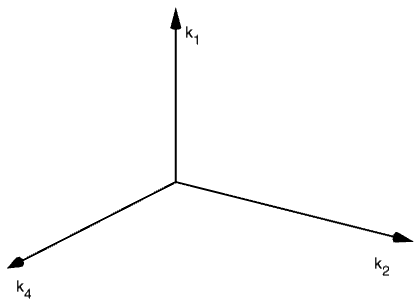
The polytope lies in a dimension space. In order to visualize it, we consider the projection onto with :
•
,
•
,
•
.
This corresponds to the restriction of with and .
We have seen that compositions of with a fixed are in bijection with the compositions of (corresponding to removing columns of height 3), so we do not lose information by considering this projection, because we know that adding such a column conjugates the type.
Moreover, when , we can still consider the points on the same object, since the points simply lie in the "inner" polytope with .
Therefore we can build the union of polytopes consisting of all points of such that , with either or . All points of occur this way, so visualizing all the , for , give us a good understanding of . Further on, we oversimplify the situation by calling these polytopes.
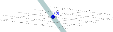
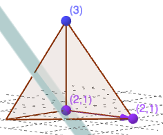
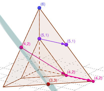
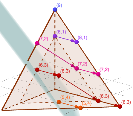
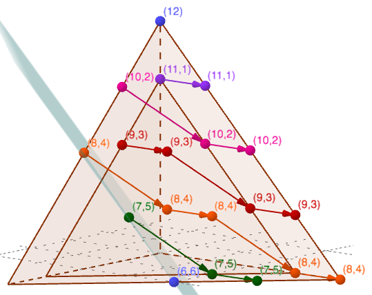
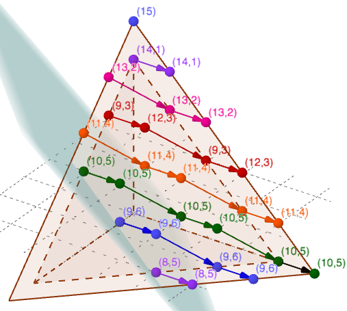
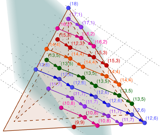
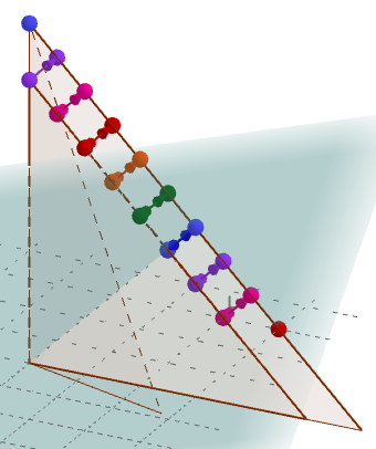
See figure 2 for the first , for . Together, they give projections of at . Figure 3 illustrates the fact that is the union of two polytopes.
Figure 2: Projections of at . The shaded plane is .
The partition strands are colored identically from one figure to the next if they occur as a shift of by . This allows to visualize how . Figure 3: Side cut of which illustrates the fact that is the union of two polytopes, an inner one with , and an outer one with . Integer points of both polytopes of the same -strand lie on the line of direction , by the geometry of transformations.
In the appendix, we give a closed formula for the number of integer points in both and . This is of interest, since they respectively give the number of tableaux of content with at most two rows, and the number of tableaux of content of any shape.
We can focus on tableaux of content with at most two parts, the ones who appear in . A partition of with at most two parts is of the form , for . We call the collection of points corresponding to tableaux of that shape in the -strand. They correspond to points such that .
As we have seen in section 5, the transformations between points which preserve the associated partition are or , depending on the value of . Therefore the points giving are linked by these transformations, and form an actual strand.
These transformations correspond precisely to exchanging a on the first row with a on the second row of the associated tableaux.
6.2 Inclusion of polytopes, complete and incomplete strands
Proposition 6.1 :
The polytope is included in for , with the strands of becoming that of .
Proof.
This injection corresponds to the operation defined in section 3. This gives a shift to all points of by adding 1 to .
∎
A -strand is called complete when this injection of into does not modify the number of tableaux it contains. The complete -strands of are associated to partitions with , and correspond to the case where . The initial point of a complete -strand corresponds to the tableau which only have ’s on the second row, and its final point, to the one which only have ’s on the second row.
For , the -strands of are incomplete. There are three tableaux in the -strand of which are not obtained from tableaux of by adding three cells with filling in their first row: the first tableau of the -strand which has no three on it’s first row, the last one which has no two’s on it’s first row, and the previous to last one, which becomes non standard when removing three cells with filling in its first row. See figure 4.
Going from to either preserve the -strands (if ) or removes three tableaux to them: one at the beginning of each -strand, and two at their end. The inclusion of in also justifies the notation of -strand, since it doesn’t modify the second part of the associated partitions, the strands depend only on the values of and .
Remark 6.2 :
The three tableaux which are removed from the -stand when going from to are removed because they do not have the form .
-strand in
-strand in
-strand in
Impossible, no ’s on the first row
Impossible, no ’s on the first row, and gives a non-partition shape.
Impossible, gives a non-semistandard tableau
Impossible, no ’s on the first row
Figure 4: Reduction of the -strand from to . The -strand is complete in , and counts tableaux. The -strand in counts only tableau, and it vanishes in .
Proposition 6.3 :
An (incomplete) -strand first appears in , grows until complete, and remains complete for with .
It holds respectively , or tableaux in its first occurrence, depending on whether or , the first one being such that and .
Proof.
Tableaux in different which have the same second row correspond to the same points of the -strand, using the inclusion. In a complete -stand, the second row of the first tableau has no ’s. After exchanges, the second row holds ’s and ’s, so this is the second row of the first tableau of the -strand at its first occurrence.
∎
We have seen in section 3 that adding three cells with entries to the first row does not change the type. If a tableau first appears in , we can keep the same type for the corresponding tableau in for .
7 Types for tableaux of content
We can use results of previous sections to define types for points in . We say is of type if and only if the corresponding tableau has type .
We can now consider the type conditions the points of must satisfy to agree with the results of previous sections. Proposition 6.1 tells us we can restrict ourselves to in .
Certain type attributions are determined, but others require choices. We discuss both, and highlight which choices appear to be the simplest and should therefore be used.
7.1 Determined type attributions
The next lemma tells us about subtypes. Recall that and have -subtype , and and have -subtype .
Lemma 7.1 :
Along a -strand of , the types have alternatingly -subtype and .
The first tableau of any complete -stands of () has -subtype , and its last tableau, -subtype
.
The first tableau of any incomplete -stands of () has -subtype
,
and its last tableau, -subtype
.
Proof.
The alternance between -subtypes follows from the fact that the parity of the number of ’s on the second row of tableaux determines the -subtype.
In the case of complete -strands, the first tableau have no entry on its second row. Then its -subtype is .
For the last tableau, it has entries on it’s second row. Therefore its -subtype depends only on the parity of .
In the case of incomplete -strands, the first tableau has entries on its second row. Therefore, the number of ’s on the second row is even when and have the same parity, and odd otherwise, which gives us the -subtypes as noted.
The last tableau has entries on its second row, so its -subtype depends only on the parity of .
∎
Using the inclusion of proposition 3.2, we see that a plethystic decomposition of for all is equivalent to coloring the points of strands of (by their type). Let’s start by examining the tableaux of which have . These lie in the "center" of the , at the junction of the planes and which mark the frontiers between and . These tableaux are the first to appear in a new -strand.
Lemma 7.2 :
In order to agree with Chen’s rule and proposition 3.2, a type is determined for the integer points (tableaux) of on the plane , according to the value of the second part of the associated partition :
Proof.
There are two points in which have for a certain : . The first lies in the strand associated to the partition , and the second, to that associated to . Therefore, the only strands with a point on the plane have second part .
Recall that a -strand appears first in for .
If , . In the first case, is even, so the unique tableau in the incomplete -strand must be of type .
In the second case, is odd, so the unique tableau in the incomplete -strand must have type . This agrees with using the parity of the number of ’s on the second row.
We have only if , so the two parts of must have the same length , and must be even.
The second row then holds entries , which has the same parity as .
For , , so the second part must be one less than the first part: , and must be odd. Therefore the two tableaux in the incomplete -strand must have type or . The first tableau of the -strand has ’s on the second row, and the second, ’s. Note that only the first rests on the plane .
In the case , is odd, so the first tableau must be associated to , and the second to . In the case , is even, so it is the opposite.
∎
7.2 Choice of order for undetermined type attributions
The new -strands of have () or () tableaux if even, and () tableaux if odd. If a new -strand holds or tableaux, their types are entirely determined as we have seen above. If it holds three tableaux, the type of the middle one is determined: if even, if odd. For the first and last attribution of the -strand, however, the two types are determined, but not which is attributed to the first or last tableau.
Moreover, going from to adds three tableaux to all incomplete -strands, one to their start, and two to their end, until they become complete. At each step, the type of one of the two tableaux added at the end of a -strand is determined, the two other types are also determined, but not the order of the attribution.
The type of the tableau added at the start of the -strand is always undetermined, so fixing a rule for the attribution of these types determines the others. Any pattern which starts with either or , alternates between both subtypes and , and ends with the wanted "middle" attribution, at , gives a type attribution which agrees with Chen’s rules and our rules.
There are infinitely many possible patterns which agree with the above conditions, however some reveal interesting patterns. We now discuss one such type attribution, and argue that it is the simplest, and most elegant, one.
7.3 Simplest type attribution
This construction rests on the choice that all first type attributions of a -strand are in turn or . It was found independantly by Mike Zabrocki and coauthors [COS+22].
Theorem 1 :
Let be a tableau of shape with entries , and entries , on its second row. Define the type of to be
.
The number of tableaux of each type coincides with Chen’s formulas. Explicitly, the coefficient of in the plethysm indexed by the standard tableau is given by .
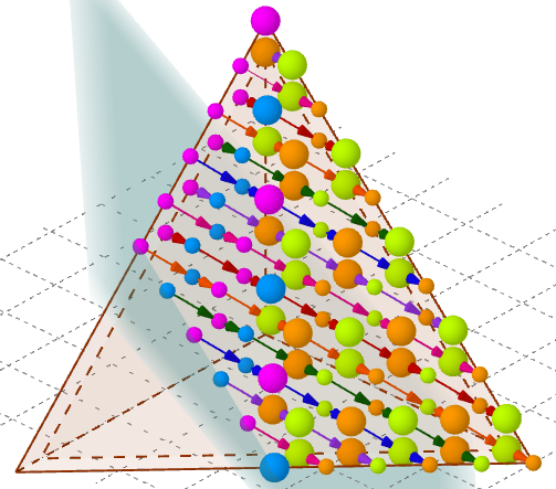
This gives the coloring of figure 5. It appears visually to be the simplest type attribution.
Figure 5: Coloring of the points of according to theorem 1, where pink points are of type , orange points, of type , green points, of type and blue points, of type . Larger points indicate points with determined type.
Remark 7.3 :
Since , the conditions account to verifying whether or , and if , what is the value of modulo .
Proof.
The complete -strands have tableaux. The first tableau of a -strand has only ’s on its second row, and each exchange increases the number of ’s on the second row by , so the last tableau has only ’s on its second row.
The condition is valid for , since , so the first tableaux have alternatingly type and . The condition is valid for , so the last tableaux have alternatingly type and .
Let’s verify we get the exact cardinalities obtained through Chen’s rules for , . Suppose , so .
We have seen that the -strand has one point on the line if , with attributions given in proposition 7.2.
Then the "middle attribution" here is , which gives
tableaux of type , tableaux of type , and tableaux of each type and . This gives exactly the cardinalities obtained through Chen’s rule for .
The proof that this is true for the other complete -strands is done using exactly the same reasoning.
Let’s now see what happens when and the -strand is incomplete in . The number of tableaux in the -strand is then .
We start by considering the types of the tableaux in the first occurrence of a -strand, verify it satisfies Chen’s rule, and verify that adding tableaux according to the attributions above also does.
At its first occurrence, a -strand counts either (), () or () tableaux. The attributions described in the proof of proposition 7.2 agree with Chen’s rule, and with the parity of the number of ’s on the second row.
Going from to adds one tableau to the start of the strand with type either or , and two tableaux to its end, of type and (in one order or the other).
When starting with one tableau, it gives four tableaux, one for each plethysms. When starting with two tableaux, it gives five tableaux, of type either ( even) or ( odd) and two times and . When starting with three tableaux, it gives six tableaux, one of each type and and two of each type and . This agrees with Chen’s rule and with the rules for -subtypes, since the attributions alternate between the two -subtypes.
Going from to then adds the six types above, and gives back the same number of tableaux modulo as in the first occurrence of the -strand. Since these attributions
agree with Chen’s rule (and with the rules for -subtypes), then all attributions do.
∎
Remark 7.4 :
This construction is particularly interesting when considering the antidiagonals appearing in : the tableaux in different strands that hold the same number of entries on their second row. They must all have the same -subtype.
In a specific antidiagonal, the attributions are segregated in two blocks, again before and after passing the threshold plane : when the number of ’s on the second line is greater to two times the number of (but not a difference of ), the type is either or (depending on the -subtype), and when it is smaller than two times the number of ’s, the type is either or . For the point with (exactly two points on each complete antidiagonal), the types are exchanged. This means that when constructing a tableau of content , there is a threshold when adding ’s to the second line after which the plethystic attribution change, and this threshold occurs when about a third of the second row holds ’s.
This also points towards a certain "stability" condition under the operation , where it preserves the plethystic attribution up to a threshold point, after which it is stable again. Proving this stability condition whould then show that the attribution described above is the unique one, as it is the only one with this property.
7.4 Other type attributions
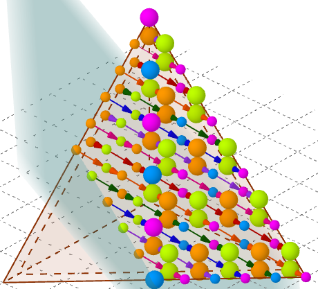
Another possible type attribution rests on the choice that all first type attributions are alternatingly and . This construction was first found by Mike Zabrocki. The resulting coloring is illustrated in figure 6. There are infinitely many other
plethystic attributions which also respect the rules discussed above.
Figure 6: Another coloring of the points of , where pink points are of type , orange points, of type , green points, of type and blue points, of type . Large points indicate determined plethystic attributions.
8 Generalizing to
All results above can be generalized to . To do so, first note that:
The Kostka numbers can be interpreted as the number of conjugate tableaux of shape and content , which are tableaux such that the entries are strictly increasing along the rows and weakly increasing along the columns. This is because each of them are obtained by conjugating a tableau of shape (i.e. reflecting it along the main diagonal).
We can understand the plethystic decomposition of by attributing types to conjugate tableaux. By using the involution introduced in section 2, we have that
So, we have that the type of a conjugate tableau is:
•
The same type as its conjugate tableau if is even;
•
The conjugate type of its conjugate tableau if is odd.
Using this, it means that our results for the plethystic decomposition of also gives the plethystic decomposition of . So, the previous results for are easily extended to .
9 Plethysm of a product of symmetric functions
Let be symmetric functions. We investigate how one can understand the plethystic decomposition of using the knowledge of the plethystic decomposition of each . It turns out that it involves an understanding of the Kronecker coefficients, which we don’t have in general. For small values of , we can compute them, and doing so, we give explicit results for . We then apply results from [MGT22] to show how to apply this technique to and . We then get an explicit plethystic decomposition of and .
9.1 The general case
Consider the symmetric function . There are two possible plethystic decompositions, depending on whether we decompose the whole product or each function separately.
In our case, we know the latter decomposition, and we want to recover the former. That is, we would like to find a map such that
We call such a map a Kronecker map. We can construct one recursively on . When , we use the following result, which can be found in [Mac98] (chapter 1, equation 7.9).
Proposition 9.1 :
For and two symmetric functions. Then:
where are the Kronecker coefficients.
These coefficients are the coefficients of in the internal product , which is defined in [Mac98] (chapter 1, section 7).
This result tells us that the map must be such that the number of pairs , where is of shape and is of shape , is equal to . This is the reason why we call a Kronecker map. Kronecker coefficients have no nice combinatorial description, so constructing such a map for all seems unlikely. However, it is doable for small values of . There are usually many choices for a Kronecker map, because Kronecker coefficients only tells us about the shape of the pairs of tableaux, not the tableaux themselves.
When , there is only one choice of Kronecker map, which is:
When , there are many possible choices. The map below is such that if , then . However this choice still doesn’t determine all pairs.
For , there is standard tableaux with cells, so there are pairs of tableaux to divide in sets. While it is not too difficult to construct a Kronecker map in that case, we can see that the difficulty increases rapidly.
Note that all possible pairs of tableaux will always appear exactly once.
Once has been found, then using proposition 9.1 recursively, we can define the map to be the map . Thus, the only difficulty to construct is to construct the map .
Example 9.2 :
Using the map as above, then:
It means that the copy of indexed respectively by tableaux and contributes to the copy of indexed by .
9.2 The case
Let be a partition. Recall that We denote
the partition where each part is repeated times. We use this notation so that .
We show how to use the plethystic decomposition of and the map from the previous section to obtain the plethystic decomposition of . This has been done in [MGT22] for , and we generalize this construction. This generalization is somewhat straightforward; see the article for a more detailed exposition.
By the Pieri rule, we have that:
We can decompose a tableau of content into a tuple of tableaux by considering subtableaux with some subsets of entries and using Schützenberger’s jeu de taquin [Sch77] to rectify them.
See [Ful96] or [Sag01] for more details about jeu de taquin and its properties. A jeu de taquin slide starts at an inner corner of the tableau, exchanges that empty cell with the cell directly under it or to its right, respecting the conditions on rows and columns for tableaux, and continues exchanges until the empty cell can no longer be moved. Below is illustrated the jeu de taquin slide starting at the inner corner in red:
Doing this until there are no more inner corners, we obtain a (straight) tableau. Schützenberger proved [Sch77] that no matter the order of the slides applied of a skew tableau , we always obtain the same rectification of , denoted . The rectification of the skew tableau above is .
Using this, let and . For , let be the skew tableau obtained by taking the cells with entries in . Then, let be the tableau obtained by subtracting to each entry; this way, has content . Finally, let . We define the decomposition to be the tuple . We can then determine the type of each according to theorem 1, and use the Kronecker map given in section 9.1 to get the type of .
It is easy to derive from results in [MGT22] that:
Proposition 9.3 :
Let be a partition and a positive integer. For , let be a tableau of content . Then, we have:
where the sum is over all of content such that .
Remark 9.4 :
In [MGT22], we construct skew tableaux , where has filling , so only the numbner of different entries differs here. This skew tableau is then rectified using jeu de taquin to obtain the straight tableau . The tableaux we sum on are then exactly tableaux of filling which are rectifications of such skew tableaux.
As a corollary, we obtain:
Corollary 9.5 :
Suppose that we know the plethystic decomposition of for all , i.e. we can attribute types to tableaux of content . Then, for any , we have
where the sum is over all tableaux of content such that if , then has type for all .
Then, by using results from the previous section, we finally obtain that:
Theorem 9.6 :
Suppose that we know the plethystic decomposition of for all , and that we know a Kronecker map (as defined in the previous section). Let be a partition and be a tableau of content . If , let be the type of . Define to be the type of . Then:
where the sum is over all tableaux of content having type .
Thus, to understand the plethystic decomposition of , we only need to understand the plethystic decomposition of (for all ) and a Kronecker map , and then apply the results of this section. This has been done in this article for , so we can understand the plethystic decomposition of . See figure 7 as an example, where the types are attributed as in section 7, and has been computed in example 9.2.
Figure 7: Attributing a type to a tableau of shape and content .
9.3 The case
The same technique can be applied to understand the plethystic decomposition of , by applying the involution. We have seen how to obtain the plethystic decomposition of from the one of in section 8, by attributing types to conjugate tableaux of content .
So we have:
Recall that counts the number of conjugate tableaux of shape and content . Let be such a conjugate tableau. As before, define to be the skew conjugate tableau obtained by taking the cells with entries in . Then, let be the skew conjugate tableau obtained by subtracting to every entry of . Finally, let (so we rectify the conjugate of , and conjugate again). We define . Then, we have the following theorem:
Theorem 9.7 :
Suppose that we know the plethystic decomposition of for all (see section 8), and that we know a Kronecker map . Let be a partition, and be a conjugate tableau of content . If , let be the type of . Define to be the type of . Then,
where the sum is over all conjugate tableaux of content having type .
This theorem is obtained by applying the involution on results of the previous section.
10 Conclusion
We have shown in this article two possible plethystic decompositions for , using various techniques. Moreover, we have shown how to extend these results to understand the plethystic decomposition of , and .
In the future, we hope to be able to understand the plethystic decomposition of . Using results in this article, it would imply a plethystic decomposition of , and by constructing a Kronecker map , of and . We also hope to be able to use these results for the plethystic decomposition of when we know the one of .
Acknowledgements
The authors are grateful to Franco Saliola for his support, and to Mike Zabrocki who shared some of his related conjectures. FMG received support from NSERC.
References
[Bri93]
Michel Brion.
Stable properties of plethysm: on two conjectures of Foulkes.
Manuscripta mathematica, 80:347–371, 1993.
[Che82]
Y.-M. Chen.
Combinatorial Algorithms for Plethysm.
PhD thesis, University of California, San Diego, 1982.
[CL93]
C. Carré and B. Leclerc.
Domino tableaux, functions and plethysms. (tableaux de dominos,
fonctions et pléthysmes.).
Séminaire Lotharingien de Combinatoire [electronic only], 31,
1993.
[COS+22]
Laura Colmenarejo, Rosa Orellana, Franco Saliola, Anne Schilling, and Mike
Zabrocki.
The mystery of plethysm coefficients, 2022.
[dB15]
Melanie de Boeck.
On the structure of Foulkes modules for the symmetric group.
PhD thesis, University of Kent, July 2015.
[dPW21]
Melanie de Boeck, Rowena Paget, and Mark Wildon.
Plethysms of symmetric functions and highest weight representations.
Transactions of the American Mathematical Society, 2021.
[Ful96]
W. Fulton.
Young Tableaux: With Applications to Representation Theory and
Geometry.
London Mathematical Society Student Texts. Cambridge University
Press, 1996.
[Lit36]
D. E. Littlewood.
Polynomial concomitants and invariant matrices.
Journal of the London Mathematical Society, s1-11(1):49–55,
1936.
[Mac98]
I.G. Macdonald.
Symmetric Functions and Hall Polynomials.
Oxford classic texts in the physical sciences. Clarendon Press, 1998.
[MGT22]
Florence Maas-Gariépy and Étienne Tétreault.
Splitting the square of homogeneous and elementary functions into
their symmetric and anti-symmetric parts, 2022.
Preprint.
[Sag01]
B. Sagan.
The Symmetric Group: Representations, Combinatorial Algorithms,
and Symmetric Functions.
Graduate Texts in Mathematics. Springer, 2001.
[Sch77]
M.-P. Schützenberger.
La correspondance de robinson.
In Dominique Foata, editor, Combinatoire et Représentation
du Groupe Symétrique, pages 59–113, Berlin, Heidelberg, 1977. Springer
Berlin Heidelberg.
[Sta12]
Richard P. Stanley.
Enumerative combinatorics. Volume 1, volume 49 of Cambridge Studies in Advanced Mathematics.
Cambridge University Press, Cambridge, second edition, 2012.
[SW85]
D.W. Stanton and D.E. White.
A Schensted algorithm for rim hook tableaux.
Journal of Combinatorial Theory, Series A, 40(2):211–247,
1985.
[Thr42]
R. M. Thrall.
On symmetrized kronecker powers and the structure of the free lie
ring.
American Journal of Mathematics, 64(1):371–388, 1942.
Appendix : Counting integer points on
The integer points on the polytope , defined in section 6 count tableaux with content , and of any shape . We have seen that can be visualized through its projection onto the union of polytopes , which represent tableaux of content , and of shape with . Figure 2 illustrates the first ’s, for . Together, they give projections onto at .
The numbers of points in these ’s are etc., which give the numbers of points in : etc.
These two series are known on the OEIS as sequences and . This interpretation of these sequences as counting tableaux however appears to be new.
Proposition A.1 :
Let . The number of integer points on is equal to the sum of integer point in all for :
The proof rests on the following lemmas. In particular, we show that the last part of the formula for gives the number of points which are added to incomplete stands when going from to .
Lemma A.2 :
Final points of strands in are integer points on lines (so or on with ( so ). In particular, and they lie on .
The position of the final point of the -strand in is if , and if .
Proof.
Let’s start by noting that all final points must lay on the lines or .
If , we can always apply the transformation , which changes the boolean value of . So final points must have , and must lie on the polytope .
If neither or (and ), then we can apply the two transformations iteratively until one or both are zero. Then no more transformations can be applied, and the final point must lie on the wanted lines. Note that if any considered starting point has , then so will the final point.
Recall that points on that give , are such that , and . Therefore, the final point of in will be such that , and .
Final point will have either , or , as seen above.
If , then and , which is greater or equal to zero if and only if .
Therefore, the partitions such that will have their final point on (), in position .
Now, if , then and , which is greater or equal to zero if and only if .
Therefore, the partitions such that will have their final point on (), in position .
∎
Remark A.3 :
Final points of will lie on when , and on otherwise.
Corollary A.4 :
The partitions with are in bijection with integer points in on the lines () and with ().
Lemma A.5 :
For fixed, the value of is given by , for the final point of the strand of in .
Proof.
We have seen that if then the final point is in position in . Then .
Similarly, if , then the final point is in position in . Then .
∎
The strands in associated with partitions with have their final points on line , and have . Therefore the number of integer points on in these strands is .
The strands associated with partitions with have their final point on the line , with . Then they have , where .
The number of point on these strands is .
This gives the wanted result for the number of points in .
As discussed above, is constructed from all the with , by letting . Therefore, we have the wanted result for as well.
∎