Spiking Neural Networks for event-based action recognition: A new task to understand their advantage

Abstract

Spiking Neural Networks (SNN) are characterised by their unique temporal dynamics, but the properties and advantages of such computations are still not well understood. In order to provide answers, in this work we demonstrate how Spiking neurons can enable temporal feature extraction in feed-forward neural networks without the need for recurrent synapses, showing how their bio-inspired computing principles can be successfully exploited beyond energy efficiency gains and evidencing their differences with respect to conventional neurons. This is demonstrated by proposing a new task, DVS-Gesture-Chain (DVS-GC), which allows, for the first time, to evaluate the perception of temporal dependencies in a real event-based action recognition dataset. Our study proves how the widely used DVS Gesture benchmark could be solved by networks without temporal feature extraction, unlike the new DVS-GC which demands an understanding of the ordering of the events. Furthermore, this setup allowed us to unveil the role of the leakage rate in spiking neurons for temporal processing tasks and demonstrated the benefits of ”hard reset” mechanisms. Additionally, we also show how time-dependent weights and normalization can lead to understanding order by means of temporal attention.

Code for the DVS-GC task is available.

1 Introduction

Research in neuromorphic computing aims at advancing artificial intelligence (AI) by extracting the computing principles behind biological neural networks. To this end, a large body of work has focused on developing Spiking neural networks (SNN), a closer approximation to real brains [1]. From an application point of view, SNN’s sparse and asynchronous computations have been demonstrated to provide great gains in energy efficiency when implemented in neuromorphic hardware [2], thus becoming their major selling point. Still, their differences with respect to conventional ANNs go beyond, as their event-driven temporal dynamics provide an alternative paradigm for temporal processing. The potential advantages of this paradigm have often been overlooked; therefore, a study demonstrating its exploitable properties demands attention.

To provide such demonstration, in this work we will make use of the task of event-based action recognition. This is motivated by the fact that SNNs are naturally suited for the processing of event-based data. These networks are able to integrate input over time and their neurons are activated in an event-based manner, hence their application to event-based data has been a topic of interest [3, 4, 5]. Additionally, given the recent surge in popularity of event-based cameras, research on event-based action recognition is a major priority, making neuromorphic video [6, 7] the perfect target.

Despite the ample variety of conventional frame-based action recognition datasets, the options for event-based action recognition are very limited [8, 3], forcing many researchers to resort to artificially generated datasets, which either convert frame sequences to events [9, 10] or generate them from simulations [11, 12]. Alternatively, those works employing real data from an event camera [13, 14, 15, 16] have mainly resorted to IBM’s DVS Gesture Dataset [3].

In this work, we prove how the action recognition task in the DVS Gesture dataset does not require processing of temporal information in order to be solved. This goes one step further than [17] where it was shown how spike timing was not relevant for N-MNIST while it was for DVS-Gesture.

To bypass the limitation of DVS Gesture, we propose DVS-Gesture-Chain (DVS-GC), a new task that can only be solved by those systems capable of perceiving the ordering of events in time. This new benchmark is based on the temporal combination of multiple gestures from the original DVS-Gesture, and allows testing the temporal perception of an action recognition system on real event-based data. Additionally, our method permits making the task arbitrarily complex in time, allowing systematic testing of the limits of a system’s memory.

Using this new task, we show how Spiking Neurons enable spatio-temporal feature extraction without the need for recurrent synapses, demonstrating a form of temporal computation which is different from the one in conventional ANNs and providing an alternative approach to time processing. We analyse the differences in this new computing paradigm with respect to conventional Recurrent Neural Networks (RNN), and further develop the current understanding of it by demonstrating the effects of membrane potential leak and reset mechanism. Specifically, we show how the reset by subtraction approach can cause slow adaptation to incoming inputs, translating to what we call a ”repetition error”. Then we prove how this can be alleviated by voltage leak or by using a reset to zero strategy, leading to improved action recognition accuracy.

Finally, we also explore the role of temporal attention when perceiving order through time-dependent weights and normalization, which implement a type of attention that is hard-coded in time.

2 Related work

2.1 Temporal processing

When processing temporal sequences of stimuli, a property of cognitive systems that is considered essential for the task is working memory, which holds information from previous events and allows to relate it to those perceived later [18, 19]. In the field of neural network engineering, working memory has historically been implemented by recurrent connections, and their memory capabilities have been further enhanced by the use of advanced memory cells such as LSTM [20] and LMU [21]. More recently, temporal processing tasks [22, 23, 24] have also been solved by the increasingly popular Transformer architectures [25]. When using these networks, temporal events are not presented in a succession as they happen, instead, multiple time-steps are accumulated (or the whole sequence in many cases) and then processed offline by the system. These approaches can be considered to implement working memory outside of the neural network by accumulating stimuli over time and then feeding them to the network together as a single input. Transformers have achieved state of the art accuracy in the majority of temporal tasks, but are limited by their computational and memory complexity, which scale as $O(L^{2})$ with the sequence length $L$ or $O(L\,logL)$ in efficient versions such as [26]. Hence, research in recurrent architectures is still of interest in order to create lighter systems with dynamic memory management.

Regarding SNNs, the state of the art in temporal tasks is based on RNN architectures. The authors in [27] proposed Recurrent SNNs (RSNNs) of Leaky integrate-and-fire (LIF) neurons with neuronal adaptation, a process that reduces the excitability of neurons based on preceding firing activity. Their resulting network is tested in the Sequential MNIST (S-MNIST) and TIMIT tasks. Subsequent work applied LSTM cells to SNN networks, achieving higher performance in S-MNIST [28].

Still, for the processing of visual event-based datasets such as DHP19 or DVS-Gesture, the state of the art is set by feed-forward SNNs with no recurrency [29, 30, 31]. The remaining question is then whether these feed-forward SNNs implement working memory or, on the contrary, the aforementioned tasks do not require temporal feature extraction. The experiments presented in this work will prove how both statements are true.

2.2 Event-based datasets

The event-based sensor market is still in its infancy and its still limited commercial adoption has not allowed to collect large volumes of event-based data. Currently, many of the datasets used in computer vision are artificially created from frame-based data or simulations. N-MNIST, N-Caltech101 [32] and DVS-CIFAR10 [33] are three popular datasets created through screen recordings of the original frame-based data with a neuromorphic camera. Alternatively, frame-based datasets have also been converted into events directly through software [9, 10, 34]. Finally, [12, 35] provide simulators for the generation of synthetic event data.

Still, the most desirable option for the development of event-based systems is to use data from a real-world acquisition. In the present day, most of the available natively neuromorphic datasets are still simple compared to traditional frame-based ones. Among them we can find N-CARS [36] a binary classification dataset, ASL-DVS [37] a 24 class sign language classification task, DHP19 [38] a 33 class pose estimation dataset, DailyActionDVS [39] a 12 class action recognition task and DVS-Gesture [3] the widely used 11 class action recognition dataset.

3 Methodology

3.1 DVS Gesture Chain

The objective is to define an action recognition task on event-based sequences that requires the perception of temporal dependencies when solving it. In order to create such temporal dependencies, the sequences to classify should be composed of a succession of smaller actions, then, the ordering of these sub-actions will have a relevant meaning for the final classification. DVS-GC achieves these requirements by leveraging the DVS-Gesture dataset and combining its gestures into chains of gestures. The result is a dataset where the classes to recognise are successions of multiple gestures and the order in which they appear is essential to its correct classification, as each possible gesture chain has a different label. This poses a challenge requiring both spatial recognition and temporal perception, where the spatial recognition part is reasonably simple, allowing to focalize evaluation on its temporal aspect.

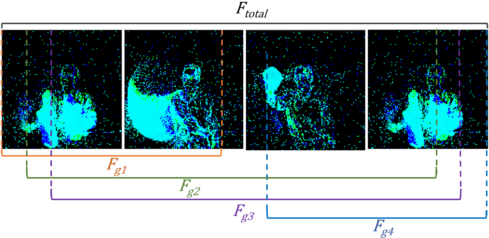
Figure 1: Example gesture chain with variable $F_{g}$ duration ($\alpha_{1}=0.2$ and $\alpha_{2}=1$). The coloured underscores represent, for each gesture in the chain, the temporal window in which they could appear given the values of $\alpha_{1}$ and $\alpha_{2}$. This allows to understand why the gesture transition is not predictable and most time-steps have no guarantees of belonging to a certain position in the chain.

3.1.1 Creation of the action classes

The creation of classes in DVS-GC is parametrized by the length of the gesture chain $L$ and the number of gestures $N$ used in the chain. Then the number of generated classes $C$ will be equal to all possible combinations (Eq. 1). Alternatively, we also provide a class generation method which does not allow to repeat the same gesture in consecutive positions of the chain, reducing the possible permutations of the chain (Eq. 2). Using different values of $N$, $L$ and the methodology with and without repetition, we created different datasets that we use to evaluate our networks (results shown in section 4).

$$C=N^{L}\\$$ (1)

$$C=N(N-1)^{L-1}$$ (2)

3.1.2 Chaining of events

Given the stream of 4-dimensional events (x, y, time, polarity) provided by the DVS-Gesture dataset, as done in most state of the art systems [40, 29, 13, 41], we transform them into frames by accumulating events in a time window. The initial number of generated frames $F$ per sequence is user defined and will be constant for all instances in the dataset. The resulting frames have two channels, one for positive polarity and one for negative.

Given that the gesture instances are obtained from a set of users under different lighting conditions, the gesture chains are created combining the gestures from the same user under the same lighting condition. This avoids sudden changes in illumination or the appearance of the user, which could help the system identify the transition between a gesture and the next. It is also worth noting that the subjects are split in the Training and Testing sets following the original DVS-Gesture split, therefore users appearing in the test set do not appear in the training set.

When building the gesture chains, having a constant number of frames for each gesture can also allow the machine to know when the transition will happen. To solve this, the duration in frames of each gesture $F_{g}$ is made variable. Let $F$ be the initial number of frames that the gesture sequences have and $F_{total}$ the target number of frames for the final gesture chains, which is user defined. Then, as seen in Eq. 3, the duration of each gesture $F_{g}$ will be a fraction of $F$ (parameterized by the coefficients $\alpha_{1}$ and $\alpha_{2}$) which satisfies that the total sum equal to $F_{total}$.

$$F_{g}\in[\alpha_{1}F,\alpha_{2}F]\mid\sum_{g=1}^{L}F_{g}=F_{total}$$ (3)

Then, the value for $F_{g}$ is chosen randomly from the set we just defined, and the resampling from $F$ to $F_{g}$ is carried out by taking the first $F_{g}$ frames of the original sequence (Fig. 1 demonstrates this variability visually). In our experiments, we define two datasets with $\alpha_{1}=0.5$ $\alpha_{2}=0.7$ and one with $\alpha_{1}=0.2$ $\alpha_{2}=1$. Both work well when using the sequences in DVS-Gesture because each gesture is repeated several times per recording, and therefore it is recognisable even after discarding a substantial part of the sequence.

Finally, when targeting a specific $F_{total}$, the number of initial frames $F$ that will allow the values of $F_{g}$ to have a uniform distribution between $\alpha_{1}F$ and $\alpha_{2}F$ is given by Eq. 4:

$$F=\frac{F_{total}}{L}\frac{2}{\alpha_{1}+\alpha_{2}}$$ (4)

3.2 Neural network architecture

For our experiments, we make use of the state of the art SNN system presented in [41], the S-ResNet, which uses a LIF neuron model and reset by subtraction [42]. The output layer is defined as a layer without leakage and without spiking activation, and its membrane potential after the last time-step provides the final class scores (complete specification in Appendix A). Apart from that, the S-ResNet uses BNTT as noramlization strategy. As seen in Eq. 5, for a time-dependent input of $d$ dimensions $x_{t}=(x_{1,t}...x_{d,t})$, the method defines an individual BN module per time-step. This not only normalizes each feature $k$ (or convolutional channel in the case of CNNs) independently, as regular BN would do, but also defines independent statistics (mean $\mu_{k,t}$ and standard deviation $\sigma_{k,t}$) and learnable weights ($\gamma_{k,t}$ and $\beta_{k,t}$) per time-step $t$.

$$BNTT(x_{k,t})=\gamma_{k,t}\frac{x_{k,t}-\mu_{k,t}}{(\sigma_{k,t})^{2}+\epsilon}+\beta_{k,t}$$ (5)

In order to compare to non-spiking ANNs, we also define a non-spiking version of the same architecture. We substitute the neuron model by the Rectified Linear Unit (ReLU) activation function, and instead of BNTT we use regular BN. With these changes, the network becomes a conventional feed-forward ResNet. These networks process the input instantaneously, without temporal dynamics, which means that, for a sequence classification task such as action recognition, they can give an output per time-step but not a global one for the whole sequence. We solve this by adding the same output layer used by the SNN, which can be seen as a voting system that accumulates the outputs for all time-steps by summing them together. We refer to this network as ANN-BN.

4 Results

In this section, we first prove how a network without the capability for temporal feature extraction (ANN-BN) can solve the classification task in DVS-Gesture but fails to do so in the new DVS-GC, which demands a perception of temporal order. We then demonstrate how, in contrast, an SNN of the same architecture learns to perceive the temporal dependencies in DVS-GC. From there, we evaluate the effects of the membrane potential reset strategy, voltage leak, time-dependent weights, and time-dependent normalization. Finally, we compare SNNs to conventional RNNs.

4.1 DVS-Gesture evaluation

Many previous works reporting accuracy performances in DVS-Gestures have taken the approach of training with the whole training set, evaluating test set performance through training epochs, and then reporting the highest test accuracy as the final test accuracy. We consider this approach to be reporting validation accuracy rather than test. Therefore, in our setup, we only evaluate the test set after training is completed, without using its value to tune the training.

Table 1 shows how both SNN and ANN achieve high accuracy in the DVS-Gestures task. As previously stated, the ANN final prediction is just a sum of the individual predictions made at each time-step. Each of these is made using the information from a frame which integrates the events received within a time window; in the case of our experiments, the time window is $\frac{1}{50}$ of the total event sequence. Given that the ANN has no way of combining information from other frames and because it has no notion of the timing in where frames happened, this means that the spatial information in the DVS-Gesture events is enough to solve the task and it is not necessary to interpret their ordering or correlation in time. This implies that the action recognition task in DVS-Gesture does not evaluate perception of temporal dependencies, and it can be solved by systems designed for the classification of static images.

Additionally, we also report the accuracy obtained by the SNN with conventional BN (SNN-BN) and the accuracy of the ANN with BNTT (ANN-BNTT). It can be seen how the ANN does not benefit from the time-dependent computations of BNTT and obtains a very similar result. On the contrary, the SNN performance decreases when using regular BN, demonstrating how, for a system where activity statistics change through time such as SNN, timing-aware normalization is beneficial.

Table 1: Test performance on DVS-Gesture. SNN* was initialized with pre-trained weights as proposed in [41]. Training and testing were run for 3 times, accuracies presented as mean ± std.

Network Normalization DVS-Gesture Accuracy SNN BN 70.31 ± 3.27 % SNN BNTT 89.82 ± 1.50% SNN* BNTT 94.84 ± 1.06 % ANN BN 97.35 ± 0.45 % ANN BNTT 96.95 ± 0.61%

4.2 DVS-Gesture-Chain evaluation

Using the methodology described in the previous section 3.1 we created three DVS-GC datasets, which are summarised in Table 2. Datasets 81-p and 96-p define a smaller variability for the duration $F_{g}$ of each individual gesture ($\alpha_{1}=0.5$, $\alpha_{2}=0.7$), while 96-u defines a larger one, making it much harder to predict the transition between gestures in time (Fig. 1 demonstrates this variability visually).

For all three, we create a validation set with 20% of the training data and evaluate it at every epoch. The test performance is then evaluated using the weights with the highest validation accuracy.

Table 2: Parameters per dataset. In the naming convention, -p stands for predictable time windows while -u stands for unpredictable time windows.

Name N L $\boldsymbol{\alpha_{1}}$ $\boldsymbol{\alpha_{2}}$ Repetition # classes 81-p 3 4 0.5 0.7 Yes (Eq. 1) 81 96-p 3 6 0.5 0.7 No (Eq. 2) 96 96-u 3 6 0.2 1 No (Eq. 2) 96

4.2.1 ANN vs SNN and time-dependent weights

We begin by evaluating the networks on the 81-p and 96-p datasets. As seen in Table 3, now that the task requires distinguishing the ordering of the events, the non-temporal ANN (ANN-BN) fails to solve it. Moreover, its accuracy value implicitly reveals the computations performed by the network: Taking the 81 class data set as an example, one can see how the ANN accuracy (16.91%±0.5) is higher than random chance (1.23%). This is because the network is capable of detecting the gestures present in the sequence and the number of times they appear, but is unable to perceive their ordering. With such conditions, and assuming a perfect accuracy in gesture detection, the probability of correctly classifying a sequence for the 81 class dataset is $p_{d}=16.05\%$ (proof in Appendix B).

Table 3: Test performance on DVS-GC. Training and testing were run for 3 times, accuracies presented as mean ± std.

Network Normalization Dataset Accuracy ANN BN 81-p 16.91 ± 0.50 % ANN BNTT 81-p 99.52 ± 0.31 % ANN None 81-p 1.24 % ANN BN + TW 81-p 89.44 ± 5.74 % ANN BN + TWC 81-p 91.08 ± 8.10 % SNN BN 81-p 86.00 ± 2.38 % SNN BNTT 81-p 95.83 ± 0.62 % SNN None 81-p 1.24 % ANN BN 96-p 12.96 ± 0.74 % ANN BNTT 96-p 99.52 ± 0.55 % SNN BN 96-p 80.62 ± 2.76 % SNN BNTT 96-p 96.32 ± 0.02 % ANN BNTT 96-u 74.66 ± 0.64 % SNN BNTT 96-u 91.16 ± 1.30 %

On the other hand, the results show how the SNN still achieves high accuracy on these same datasets, implying that its temporal dynamics allow to perceive order in time. In order to analyse which components of the network enable this capacity, we also test the performance of the SNN with conventional BN (SNN-BN) and the accuracy of the ANN with BNTT (ANN-BNTT). The accuracies obtained by both systems indicate that they are successfully learning to perceive order, meaning that both, spiking neurons and BNTT can enable a neural network to recognise temporal sequences on their own. Additionally, it is also worth noticing how, for the 81-p and 96-p datasets, the ANN with BNTT is more accurate than the SNN.

In BNTT, the perception of order is gained by learning time-dependent values that are used to scale the activation maps of the network, providing temporal attention. In order to decorrelate this capacity from the normalization strategy, we create a modified version of the non-temporal ANN with regular BN that we call ANN-TW (ANN with temporal weight). This version adds a learnable weight $w_{l,t}\in\mathbb{R}^{1}$ per time-step $t$ at each layer $l$, which is used to scale the activation map after the convolution (Conv) and BN layers as: $y_{l,t}=BN(Conv(x_{l,t}))\cdot w_{l,t}$. Additionally, because BNTT learns independent parameters for each channel, we also define an alternative version (ANN-TWC) where each channel learns a different temporal weight.

The performance of ANN-TW (Table 3) proves how a single time-dependent weight per layer is enough to recognise the temporal sequences in 81-p and how the learned value does not need to be different between channels for temporal perception purposes. Still, the ANN-TWC obtains a slightly higher accuracy. Apart from that, the performances of both networks are lower to those of the systems using time-dependent normalization statistics, proving how these are not essential but indeed beneficial. A BNTT ablation study is available in Appendix C.

Finally, we evaluate the performances of the networks with the 96-u configuration, where the variability of the duration $F_{g}$ of each individual gesture is higher. The results (last two rows of Table 3) demonstrate how this set-up greatly decreases the performance of the ANN-BNTT, meaning that temporal attention is not enough for the task. In contrast, SNN-BNTT exhibits a smaller decrease and still solves the task with high accuracy, proving how the capacity of SNNs for spatio-temporal feature extraction goes beyond that of temporal attention. The complete analysis justifying these results is provided in Section 5.

4.2.2 Leak and reset mechanism

When using regular BN, the SNN does not have temporal weights, making voltage leak the only time-aware component in the network. This motivates us to explore its relevance to solving the task.

Table 4 compares the results of the same network trained with LIF neurons and IF neurons (no leak). Because the performance comparison between LIF and IF can be affected by the chosen leak coefficient, we searched for its optimal value through hyper-parameter search. We find the best results with $0.87$ for the 81 class dataset and $0.80$ for the 96 class one.

The original network, which uses reset by subtraction, suffers a major performance drop when not equipped with leak. We found that the reason behind this is the excess of voltage in neurons reset by subtraction, which can trigger delayed spikes that slow down adaptation to newer inputs. We quantify this effect by means of what we call ”repetition error” (R-error). The R-error is measured as the percentage of wrong classifications where at least one of the miss-classified gestures in the chain has been predicted to be the same as the preceding one. As there are three different gestures to choose from at each position in the chain, the standard R-error is 33.3%. Values higher than this one will indicate a tendency towards repeating previous predictions. (Notice that the 96-class dataset does not allow repetition in its classes and therefore cannot present R-error, still, not clearing old voltage also decreases the performance in it)

These results demonstrate how voltage leak prevents old information from corrupting current calculations. In addition to that, we evaluated how a reset to zero strategy can also prevent this same issue (Table 4). Interestingly, reset to zero consistently achieves the best performance when paired with IF neurons, while implementing leak decreases its accuracy.

Table 4: Test accuracy and R-error of the SNN-BN under different setups. IF neurons do not leak. Zero stands for reset to zero and Sub for subtraction. LIF neurons use a leakage factor of 0.87 except for LIF-Sub in 96-u, which uses 0.80. Training and testing were run for 3 times, accuracies presented as mean ± std.

Neuron Reset Dataset Accuracy R-error LIF Sub 81-p 86 ± 2.38 % 33.54 ± 5.20 % IF Sub 81-p 48.27 ± 1.38 % 70.41 ± 2.44 % LIF Zero 81-p 82.31 ± 2.14 % 35.30 ± 8.09 % IF Zero 81-p 92.59 ± 2.67 % 31.01 ± 2.15 % LIF Sub 96-u 68.74 ± 1.45 % n/a LIF Zero 96-u 63.58 ± 3.09 % n/a IF Zero 96-u 71.40 ± 4.55 % n/a

4.2.3 RNN vs SNN

After demonstrating how SNNs can perform temporal computations without the need for recurrent connections, we further validate our results by comparing their performance with that of RNNs. For this, we define a different architecture based on a non-spiking ResNet14, which acts as spatial feature extractor, and append (1 or 2) fully connected ”temporal layers” of 128 features before the final classification layer, to act as temporal feature extractor. As temporal layers we test feed-forward SNN layers, recurrent SNN layers (RSNN), vanilla RNN and LSTM.

Table 5 shows how, for 96-u, SNNs outperform vanilla RNNs while LSTMs outperform SNNs. The RSNN demonstrates a substantial improvement with respect to the SNN when using two layers, getting closer to the LSTM performance. On the other hand, in the dataset with predictable time windows, 81-p, all networks perform at a similar level, implying that all networks manage to exploit its predictable time windows, arguably, demonstrating time-dependent feature extraction.

The performance differences between SNN, RSNN, RNN, and LSTM are well justified by their computing principles, which we analyse in section 5.2.1.

Table 5: Test accuracy in DVS-GC 81-p and 96-u. SNNs use IF neurons and reset to zero. Training and testing were run for 3 times, accuracies presented as mean ± std. ”# TL” stands for number of temporal layers.”# params” presents the number of parameters used in the temporal layers as a factor of the parameters of a 128-dimensional dense layer. *RNN presents the maximum accuracy instead of the mean, as numerous trials failed to learn.

Temporal layers # TL # params Dataset Accuracy SNN 1 $\times$1 96-u 61.53 ± 3.27 % SNN 2 $\times$2 96-u 67.09 ± 1.57 % RSNN 1 $\times$2 96-u 64.62 ± 0.69 % RSNN 2 $\times$4 96-u 77.80 ± 1.92 % RNN 1 $\times$2 96-u 44.08* % RNN 2 $\times$4 96-u 65.58* % LSTM 1 $\times$8 96-u 87.31 ± 2.79 % LSTM 2 $\times$16 96-u 88.80 ± 3.47 % SNN 2 $\times$2 81-p 84.60 ± 3.08 % RSNN 2 $\times$4 81-p 86.47 ± 1.44 % RNN 2 $\times$4 81-p 72.32 ± 16.91 % LSTM 2 $\times$16 81-p 89.83 ± 3.34 %

5 Analysis of temporal computations

After proving through empirical results how spiking neurons and time-dependent weights enable temporal order perception, in this section we analyse the in-depth mechanics that implement this capability.

5.1 Temporal attention analysis

Networks with time-dependent weights such as ANN-TW or those using BNTT use temporal attention to store the time at which a visual detection occurred. This is achieved by constraining the activation of certain layers or channels to a time window, then the feature detected by those neurons will be known to happen within that time-window.

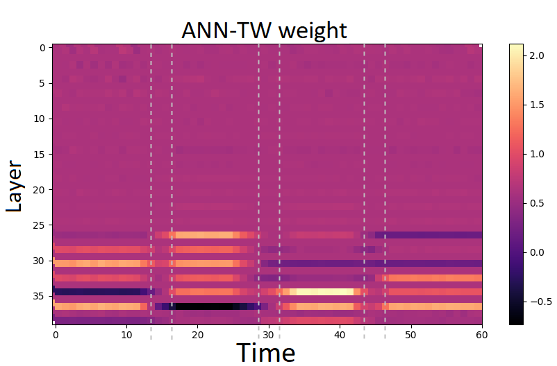
Figure 2: Value of the time weight in TW-ANN. Dotted lines highlight the gesture transition zone. The last two layers of the graph correspond to the layers in the residual connection downsampling. Trained in the 81-p DVS-GC.

In order to prove how the networks are using this strategy, in Fig. 2, we visualize the value of the temporal weight in ANN-TW when trained in the 81-p dataset. Notice that, when designing DVS-GC, we made the gesture chaining procedure variable in time, so that the transition between gestures does not always happen in the same time-step. Now, visualising the graph, it can be seen how the network learned to reduce the weight in the uncertainty zone of the transition and defined its detection time windows between the time-steps which are guaranteed to belong to the n-th gesture. Then, we observe how the weight restricts the last layers to only be active in time windows corresponding to specific positions in the 4-gesture chain. This specializes different layers in detecting gestures at certain positions in the chain, acting as a temporal attention coefficient. This is equivalent to associating timestamps to the detected spatial features and then combining this information in the last layer by accumulation. This last layer is the only element in the system implementing memory for the non-spiking networks. The same principle was proven for BNTT in Appendix D.

Given this computational logic, it is then clear why in the 96-u dataset the performance of these networks dropped. With $\alpha_{1}=0.2$ and $\alpha_{2}=1$ time-steps are not guaranteed to contain a specific position in the chain (except for the first and last gestures), since the transition zones now overlap. Therefore, in that scenario, time-dependent features calculated using temporal attention are not a reliable descriptor.

5.2 Spiking neuron analisys

Unlike temporal attention, spiking neurons achieve high accuracy in all three datasets. This shows how SNN can perform two types of spatio-temporal tasks:

1. Sequence recognition with predictable action time windows in the 81-p dataset.

2. Sequence recognition with unpredictable time windows in the 96-u dataset.

Task 1 can be solved by means of time-dependent features, as shown by the analysis performed on temporal weights. Moreover, as this dataset allows repetition, these kind of features are indispensable in order to distinguish individual gestures when the same one is repeated in succession.

Task 2, to the best of our knowledge, can only be solved by recognising each gesture transition in the chain, as the timing of an action is not enough to find its chain location and, therefore, the relative order of appearance is the only usable information.

Following that logic, by performing successfully in Task 2, SNNs demonstrate that they can detect gesture transitions in a time-invariant manner, while in Task 1, they demonstrate the ability to localise gestures in time. Such behaviour implies that spiking neurons enable time-invariant spatio-temporal feature extraction as well as time-dependent feature extraction.

5.2.1 Comparing SNN to RNN

A layer of spiking neurons can be seen as a recurrent cell where the current input $x_{t}$ passes through a layer and is summed to the previous state $v_{t-1}$. The contribution of $v_{t-1}$ is weighted by the leak factor, and the final voltage $v_{t}$ is decreased by subtracting voltage in the event of a spike. Therefore, they retain memory by integrating inputs over time until the threshold is surpassed. Then, when the information is released in form of a spike, it is deleted from memory through the reset mechanism. On the contrary, in a non-spiking vanilla RNN, the neuron itself has no memory, recurrency is implemented only at layer level by defining a recurrent synapse from each neuron to itself and lateral synapses within the layer. Therefore, it is to be expected for SNN/RSNN to have better performance than RNNs.

On the other hand, LSTM adds a cell state to their computations to integrate inputs through time, like spiking neurons do, but, as seen in Figure 3, it has three differences: First, the integration is weighted by two gating layers, the input and forget gates, while LIF neurons compute which information to forget through the reset mechanism and the leak factor. Second, in LSTM the non-linearity is applied before integration, while the spiking neuron applies its non-linearity (thresholding) only to the output. Finally, in an LSTM the output is weighted by another gating layer.

This side by side comparison illustrates how spiking neurons define a computing principle similar to LSTM units, but without the use of gating layers, resulting in a lighter network. Additionally, it allows to understand how, as seen in the experiments, an internal state can be enough to calculate temporal features. Recurrent connections can be beneficial, but they are not indispensable.

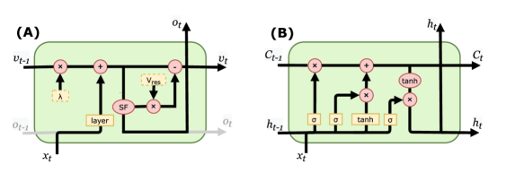
Figure 3: (A): Diagram of a layer of LIF neurons. $layer$ are the synaptic weights, $SF$ the spiking function, $V_{res}$ the voltage reset value. Gray lines show the architecture with recurrent connections, without them, the architecture is feed-forward. (B): LSTM diagram. $C_{t}$ is the cell state, $h_{t}$ the hidden state and output, the yellow $tanh$ is a layer of synaptic weights with Hyperbolic Tangent activation. $\sigma$ stands for the gating layer with Sigmoid activation.

6 Discussion

In this work, we showed how spiking neurons can be exploited to solve temporal tasks without the need of recurrent synapses. This proves how their temporal dynamics are not only a vehicle for computational efficiency, but also a tool for the extraction of temporal features. This can allow to bypass the need for recurrent connections when a lighter network is needed and to reuse feed-forward networks for temporal tasks. Moreover, the parallelism drawn between LSTM and SNN allows to appreciate how SNN computation is closer to LSTM than to vanilla RNNs. Understanding their similarities and differences allows to make informed choices when designing temporal processing systems and paves the way to distilling more biologically inspired principles into machine learning. Additionally, it also contributes to closing the gap between neuroscience and machine learning knowledge.

In our experiments, we evaluated the two components that allow an SNN to clean its memory, the leak and reset mechanism. The effect of the leak factor has been previously evaluated in static data [43], but understanding its relevance for temporal computations was still necessary. Our results contribute to develop this understanding by showing how voltage leak prevents old information from stagnating in the network when using reset by subtraction. Looking at the reset strategy, we find that zero-reset also solves the aforementioned problem. Reset by subtraction has been a popular option given that it prevents loss of information, and has been proved especially useful in ANN to SNN conversion approaches [44]. Still, our results indicate that retaining such information can come at the cost of slower adaptation to dynamic inputs. Therefore, we believe that this effect should be taken into account when designing SNNs for temporal processing tasks, and appropriately handling it will lead to improved results, as shown in our experiments.

Additionally, the analysis of temporal weights demonstrated a clear use case for temporal attention, showing how time-dependent features are learned by a network when the meaning of the events is dictated by their timing. In this work, the implementation of temporal weights and time-dependent normalization requires learning a parameter per time-step, which would be a limitation for inputs of variable length. Still, it is enough to demonstrate the aforementioned computing principle. Moreover, it serves as a tool to prove which tasks can be solved with time-dependent features without the need for time-invariant ones.

These insights were obtained thanks to the newly proposed DVS-GC, a task which was created by means of a novel chaining technique. The relevance of this task is that, first, it fulfils the current need for event-based action recognition datasets. Apart from that, it provides an approach that allows the creation of controlled scenarios in order to evaluate specific capacities of a learning system. The datasets built in this work serve as examples, where 81-p and 96-p could be solved by timing-aware features, and 96-u could only be solved with time-invariant spatio-temporal features. Moreover, the chains can be made arbitrarily long, which allows to test the limits of a system’s memory. Looking ahead, the results provided in the proposed DVS-GC configurations can serve as a baseline when evaluating new systems. Apart from that, if a more challenging task is needed, the method allows to build longer sequences with more gestures.

Appendix

Appendix A Neural Network architecture

Here we present the full specifications of the implemented neural network and the neuron model.

The neurons in the SNN are defined by the LIF neuron model. Let $i$ be a post-synaptic neuron, $u_{i,t}$ its membrane potential, $o_{i,t}$ its spiking activation and $\lambda$ the leak factor (which we set to 0.874 following the original S-ResNet paper, unless specified otherwise). The index $j$ represents the pre-synaptic neuron and the weights $w_{i,j}$ dictate the value of the synapses between neurons. Then, the iterative update of the neuron activation is calculated as follows:

$$o_{i,t}=g\left(\sum_{j}(w_{i,j}o_{j,t})\ +\lambda\cdot u_{i,t-1}\right)$$ (6)

where $g(x)$ is the thresholding function, which converts voltage to spikes:

$$g(x)=\begin{cases}&\text{1, if }x\geq U_{th}\\ &\text{0, if }x<U_{th}\end{cases}$$ (7)

After spiking, a reset is performed by the subtraction $u_{i,t}^{*}=u_{i,t}-U_{th}$, where $u_{i,t}^{*}$ is the membrane potential after resetting. In experiments using zero reset, $u_{i,t}^{*}=0$.

We use a Spikes to Spikes (S2S) implementation for the residual connection and the output layer is defined as a layer without leakage ($\lambda=1$) and without spiking activation ($U_{th}=\infty$). This output layer accumulates the network output through all time-steps and its voltage $u_{i,t}$ at the last time-step $t=T$ provides the final class scores (Eq. 8). At training time, these are compared to the ground truth labels by means of a cross-entropy loss and the network is trained by Backpropagation Through Time (BPTT), using Stochastic Gradient Descent with a momentum of 0.9.

$$u_{i,T}=\sum_{t}^{T}\sum_{j}(w_{i,j}o_{j,t})$$ (8)

Given the non-differentiability of the thresholding function, a triangle shaped surrogate gradient is used as its derivative (Eq. 9). We use $\alpha=0.3$.

$$\frac{\partial o_{t,i}}{\partial u_{t,i}}=\alpha\max\{0,1-|u_{t,i}|\}$$ (9)

We use a depth of 38 layers and a width of 32 base filters unless otherwise specified. Training was performed using 4 Nvidia GeForce GTX 1080 Ti GPUs.

Appendix B Proof for the probability of correct classification without order perception

Assume a system with perfect gesture classification but no perception of order that is evaluated in DVS-GC. This system will know which gestures are present in the sequence and the number of times they appear, but will be unable to perceive their ordering.

For this system, depending on the number of detected gestures, the candidates to be the correct output are reduced. Therefore, to calculate its accuracy, we can calculate the probability of correctly classifying each individual class $x_{i}$ in the dataset and then, assuming a constant number of class examples, their average will be the final accuracy.

We calculate this for the 81-class DVS-GC dataset in equation 10.

$$p(x)=\begin{cases}&1\text{, if gesture repeated 4 times }\\ &\frac{1}{4}\text{, if gesture repeated 3 times }\\ &\frac{1}{6}\text{, if 2 gestures repeated 2 times }\\ &\frac{1}{36}\text{, otherwise }\end{cases}$$

$$P_{d}=\frac{1}{C}\sum_{i}^{C}p(x_{i})=$$

$$=\frac{1}{81}(3\cdot 1+24\cdot\frac{1}{4}+18\cdot\frac{1}{6}+36\cdot\frac{1}{36})=0.1605$$ (10)

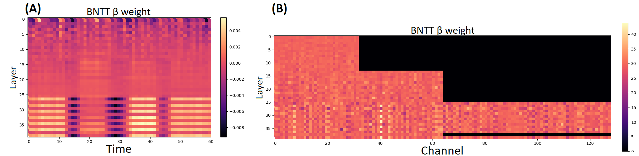
Figure 4: (A): Bias weight average value across channels in the BNTT layers of ANN-BNTT. (B): Value of the center of mass in the time dimension (60 time-steps) of the bias weight of the BNTT layers in ANN-BNTT. The last two layers of all graphs correspond to the layers in the residual connection downsampling. Trained in the 81-class DVS-GC.

Appendix C BNTT Ablation study

The BNTT module has 4 time-varying parameters, namely mean, variance, $\gamma$ weight and $\beta$ weight. In order to analyse their role in temporal understanding, we perform an ablation study where we eliminate the temporal dimension of some of this components by averaging across all time-steps. This allows to isolate the temporal performance of individual components and evaluate the accuracy degradation. Note that the experiment is performed by first training the regular network and then averaging the necessary parameters, with no retraining after the ablation.

Table 6 presents the results for each of the 4 BNTT parameters in isolation (all the other parameters were averaged in time). It can be seen how any of them is enough to maintain accuracy well above 16.05%, meaning that they all encode part of the temporal attention learned by the network. Still, there is a clear difference in accuracy between them, with $\gamma$ and $\beta$ weights having the highest accuracy and the mean having the lowest one. Of course, after averaging all of them, the network falls back to the performances seen by the ANN with regular BN.

Table 6: Test accuracy of the ANN-BNTT after averaging certain components through time. ”Non-averaged components” indicates which parts have not been averaged and therefore are still time-dependent.

Non-averaged components Accuracy Full BNTT 99.16 % $\beta$ weight 97.63 % $\gamma$ weight 93.77 % Variance 72.24 % Mean 35.96 % None 17.09 %

Appendix D BNTT’s temporal attention

Following on the study presented in section 4.2.1, we analyse the temporal attention in BNTT. Fig. 4.A displays the value of BNTT’s $\beta$ weight, which scales neuron activations. Unlike the ANN-TW graph, this one does not show large changes in the coefficient value. This is because the $\beta$ weight has a different value per channel, something that is not visible in Fig. 4.A, as it averages through channels. Therefore, in order to visualize the temporal windowing of the BNTT weight, in Fig. 4.B we plot the center of mass $m$ in the time dimension for the weights at each channel as:

$$m=\frac{1}{T}\sum_{t}^{T}(x_{t}-min(x))t$$ (11)

Where $x$ is a vector that contains a weight value $x_{t}$ per time-step $t$.

With a uniform distribution of weight through the time-steps, the center of mass would have a value equal to $T/2$, which in the case of our network would be 30. Consequently, all the values in Fig. 4.B that are far from this number are indicators of the existence of a time window. It can be seen how the centre of mass varies among different channels, demonstrating how they specialise on detecting features inside different temporal windows. This proves how BNTT hard-codes a different temporal attention for each channel in a layer.

References

- [1] Wolfgang Maass. Networks of spiking neurons: the third generation of neural network models. Neural networks, 10(9):1659–1671, 1997.
- [2] Mike Davies, Andreas Wild, Garrick Orchard, Yulia Sandamirskaya, Gabriel A Fonseca Guerra, Prasad Joshi, Philipp Plank, and Sumedh R Risbud. Advancing neuromorphic computing with loihi: A survey of results and outlook. Proceedings of the IEEE, 109(5):911–934, 2021.
- [3] Arnon Amir, Brian Taba, David J. Berg, Timothy Melano, Jeffrey L. McKinstry, Carmelo di Nolfo, Tapan Kumar Nayak, Alexander Andreopoulos, Guillaume Garreau, Marcela Mendoza, Jeffrey A. Kusnitz, Michael V. DeBole, Steven K. Esser, Tobi Delbrück, Myron Flickner, and Dharmendra S. Modha. A low power, fully event-based gesture recognition system. 2017 IEEE Conference on Computer Vision and Pattern Recognition (CVPR), pages 7388–7397, 2017.
- [4] Alexander Kugele, Thomas Pfeil, Michael Pfeiffer, and Elisabetta Chicca. Efficient processing of spatio-temporal data streams with spiking neural networks. Frontiers in Neuroscience, 14:439, 2020.
- [5] Paul Kirkland, Davide Manna, Alex Vicente-Sola, and Gaetano Di Caterina. Unsupervised spiking instance segmentation on event data using stdp features. IEEE Transactions on Computers, 2022.
- [6] Patrick Lichtsteiner, Christoph Posch, and Tobi Delbruck. A 128 128 120 db 15 s latency asynchronous temporal contrast vision sensor. IEEE Journal of Solid-State Circuits, 43(2):566–576, 2008.
- [7] Tobi Delbrück, Bernabé Linares-Barranco, Eugenio Culurciello, and Christoph Posch. Activity-driven, event-based vision sensors. Proceedings of 2010 IEEE International Symposium on Circuits and Systems, pages 2426–2429, 2010.
- [8] Junhaeng Lee, Tobi Delbrück, Michael Pfeiffer, Paul K. J. Park, Chang-Woo Shin, Hyunsurk Ryu, and Byung-Chang Kang. Real-time gesture interface based on event-driven processing from stereo silicon retinas. IEEE Transactions on Neural Networks and Learning Systems, 25:2250–2263, 2014.
- [9] Yin Bi and Yiannis Andreopoulos. Pix2nvs: Parameterized conversion of pixel-domain video frames to neuromorphic vision streams. 2017 IEEE International Conference on Image Processing (ICIP), pages 1990–1994, 2017.
- [10] Daniel Gehrig, Mathias Gehrig, Javier Hidalgo-Carri’o, and Davide Scaramuzza. Video to events: Recycling video datasets for event cameras. 2020 IEEE/CVF Conference on Computer Vision and Pattern Recognition (CVPR), pages 3583–3592, 2020.
- [11] Elias Mueggler, Henri Rebecq, Guillermo Gallego, Tobi Delbrück, and Davide Scaramuzza. The event-camera dataset and simulator: Event-based data for pose estimation, visual odometry, and slam. The International Journal of Robotics Research, 36:142 – 149, 2017.
- [12] Henri Rebecq, Daniel Gehrig, and Davide Scaramuzza. Esim: an open event camera simulator. In Aude Billard, Anca Dragan, Jan Peters, and Jun Morimoto, editors, Proceedings of The 2nd Conference on Robot Learning, volume 87 of Proceedings of Machine Learning Research, pages 969–982. PMLR, 29–31 Oct 2018.
- [13] Wei Fang, Zhaofei Yu, Yanqi Chen, Timothée Masquelier, Tiejun Huang, and Yonghong Tian. Incorporating learnable membrane time constant to enhance learning of spiking neural networks. In Proceedings of the IEEE/CVF International Conference on Computer Vision, pages 2661–2671, 2021.
- [14] Davide L Manna, Alex Vicente-Sola, Paul Kirkland, Trevor J Bihl, and Gaetano Di Caterina. Simple and complex spiking neurons: perspectives and analysis in a simple stdp scenario. Neuromorphic Computing and Engineering, 2(4):044009, 2022.
- [15] S. Shrestha and Garrick Orchard. Slayer: Spike layer error reassignment in time. In NeurIPS, 2018.
- [16] Yannan Xing, Gaetano Di Caterina, and John Soraghan. A new spiking convolutional recurrent neural network (scrnn) with applications to event-based hand gesture recognition. Frontiers in neuroscience, 14:590164, 2020.
- [17] Laxmi R Iyer, Yansong Chua, and Haizhou Li. Is neuromorphic mnist neuromorphic? analyzing the discriminative power of neuromorphic datasets in the time domain. Frontiers in neuroscience, 15:608567, 2021.
- [18] Adele Diamond. Executive functions. Annual review of psychology, 64:135–168, 2013.
- [19] Nelson Cowan. What are the differences between long-term, short-term, and working memory? Progress in brain research, 169:323–338, 2008.
- [20] Sepp Hochreiter and Jürgen Schmidhuber. Long short-term memory. Neural computation, 9(8):1735–1780, 1997.
- [21] Aaron Voelker, Ivana Kajić, and Chris Eliasmith. Legendre memory units: Continuous-time representation in recurrent neural networks. Advances in neural information processing systems, 32, 2019.
- [22] Sho Takase and Shun Kiyono. Lessons on parameter sharing across layers in transformers. arXiv preprint arXiv:2104.06022, 2021.
- [23] Haoyi Zhou, Shanghang Zhang, Jieqi Peng, Shuai Zhang, Jianxin Li, Hui Xiong, and Wancai Zhang. Informer: Beyond efficient transformer for long sequence time-series forecasting. In Proceedings of AAAI, 2021.
- [24] Chen Wei, Haoqi Fan, Saining Xie, Chao-Yuan Wu, Alan Yuille, and Christoph Feichtenhofer. Masked feature prediction for self-supervised visual pre-training. arXiv preprint arXiv:2112.09133, 2021.
- [25] Ashish Vaswani, Noam Shazeer, Niki Parmar, Jakob Uszkoreit, Llion Jones, Aidan N Gomez, Łukasz Kaiser, and Illia Polosukhin. Attention is all you need. Advances in neural information processing systems, 30, 2017.
- [26] Nikita Kitaev, Łukasz Kaiser, and Anselm Levskaya. Reformer: The efficient transformer. arXiv preprint arXiv:2001.04451, 2020.
- [27] Guillaume Bellec, Darjan Salaj, Anand Subramoney, Robert Legenstein, and Wolfgang Maass. Long short-term memory and learning-to-learn in networks of spiking neurons. Advances in neural information processing systems, 31, 2018.
- [28] Ali Lotfi Rezaabad and Sriram Vishwanath. Long short-term memory spiking networks and their applications. In International Conference on Neuromorphic Systems 2020, pages 1–9, 2020.
- [29] Hanle Zheng, Yujie Wu, Lei Deng, Yifan Hu, and Guoqi Li. Going deeper with directly-trained larger spiking neural networks. In AAAI, 2021.
- [30] Wei Fang, Zhaofei Yu, Yanqi Chen, Tiejun Huang, Timothée Masquelier, and Yonghong Tian. Deep residual learning in spiking neural networks. Advances in Neural Information Processing Systems, 34, 2021.
- [31] Youngeun Kim and Priyadarshini Panda. Optimizing deeper spiking neural networks for dynamic vision sensing. Neural Networks, 144:686–698, 2021.
- [32] Garrick Orchard, Ajinkya Jayawant, Gregory K Cohen, and Nitish Thakor. Converting static image datasets to spiking neuromorphic datasets using saccades. Frontiers in neuroscience, 9:437, 2015.
- [33] Hongmin Li, Hanchao Liu, Xiangyang Ji, Guoqi Li, and Luping Shi. Cifar10-dvs: an event-stream dataset for object classification. Frontiers in neuroscience, 11:309, 2017.
- [34] Alex Zihao Zhu, Ziyun Wang, Kaung Khant, and Kostas Daniilidis. Eventgan: Leveraging large scale image datasets for event cameras. In 2021 IEEE International Conference on Computational Photography (ICCP), pages 1–11. IEEE, 2021.
- [35] Damien Joubert, Alexandre Marcireau, Nic Ralph, Andrew Jolley, André van Schaik, and Gregory Cohen. Event camera simulator improvements via characterized parameters. Frontiers in Neuroscience, page 910, 2021.
- [36] Amos Sironi, Manuele Brambilla, Nicolas Bourdis, Xavier Lagorce, and Ryad Benosman. Hats: Histograms of averaged time surfaces for robust event-based object classification. In Proceedings of the IEEE Conference on Computer Vision and Pattern Recognition, pages 1731–1740, 2018.
- [37] Yin Bi, Aaron Chadha, Alhabib Abbas, Eirina Bourtsoulatze, and Yiannis Andreopoulos. Graph-based object classification for neuromorphic vision sensing. In Proceedings of the IEEE/CVF International Conference on Computer Vision, pages 491–501, 2019.
- [38] Enrico Calabrese, Gemma Taverni, Christopher Awai Easthope, Sophie Skriabine, Federico Corradi, Luca Longinotti, Kynan Eng, and Tobi Delbruck. Dhp19: Dynamic vision sensor 3d human pose dataset. In Proceedings of the IEEE/CVF conference on computer vision and pattern recognition workshops, pages 0–0, 2019.
- [39] Qianhui Liu, Dong Xing, Huajin Tang, De Ma, and Gang Pan. Event-based action recognition using motion information and spiking neural networks. In Zhi-Hua Zhou, editor, Proceedings of the Thirtieth International Joint Conference on Artificial Intelligence, IJCAI-21, pages 1743–1749. International Joint Conferences on Artificial Intelligence Organization, 8 2021. Main Track.
- [40] Jacques Kaiser, Hesham Mostafa, and Emre Neftci. Synaptic plasticity dynamics for deep continuous local learning (decolle). Frontiers in Neuroscience, 14:424, 2020.
- [41] Alex Vicente-Sola, Davide Liberato Manna, Paul Kirkland, Gaetano Di Caterina, and Trevor J Bihl. Keys to accurate feature extraction using residual spiking neural networks. Neuromorphic Computing and Engineering, 2022.
- [42] Andrew S. Cassidy, Paul Merolla, John V. Arthur, Steve K. Esser, Bryan Jackson, Rodrigo Alvarez-Icaza, Pallab Datta, Jun Sawada, Theodore M. Wong, Vitaly Feldman, Arnon Amir, Daniel Ben-Dayan Rubin, Filipp Akopyan, Emmett McQuinn, William P. Risk, and Dharmendra S. Modha. Cognitive computing building block: A versatile and efficient digital neuron model for neurosynaptic cores. In The 2013 International Joint Conference on Neural Networks (IJCNN), pages 1–10, 2013.
- [43] Sayeed Shafayet Chowdhury, Chankyu Lee, and Kaushik Roy. Towards understanding the effect of leak in spiking neural networks. Neurocomputing, 464:83–94, 2021.
- [44] Bodo Rueckauer, Iulia-Alexandra Lungu, Yuhuang Hu, Michael Pfeiffer, and Shih-Chii Liu. Conversion of continuous-valued deep networks to efficient event-driven networks for image classification. Frontiers in Neuroscience, 11, 2017.