Learning Low-Frequency Motion Control for
Robust and Dynamic Robot Locomotion

Abstract

Robotic locomotion is often approached with the goal of maximizing robustness and reactivity by increasing motion control frequency. We challenge this intuitive notion by demonstrating robust and dynamic locomotion with a learned motion controller executing at as low as $8\text{\,}\mathrm{Hz}$ on a real ANYmal C quadruped. The robot is able to robustly and repeatably achieve a high heading velocity of $1.5\text{\,}\mathrm{m}\text{\,}{\mathrm{s}}^{-1}$, traverse uneven terrain, and resist unexpected external perturbations. We further present a comparative analysis of deep reinforcement learning (RL) based motion control policies trained and executed at frequencies ranging from $5\text{\,}\mathrm{Hz}$ to $200\text{\,}\mathrm{Hz}$. We show that low-frequency policies are less sensitive to actuation latencies and variations in system dynamics. This is to the extent that a successful sim-to-real transfer can be performed even without any dynamics randomization or actuation modeling. We support this claim through a set of rigorous empirical evaluations. Moreover, to assist reproducibility, we provide the training and deployment code along with an extended analysis at https://ori-drs.github.io/lfmc/.

I Introduction

Legged systems can execute agile motions by leveraging their ability to reach appropriate and disjoint support contacts, thereby enabling outstanding mobility in complex and unstructured environments. This, however, requires control solutions that are able to recover from unexpected perturbations, adapt to variations in system and environment dynamics, and execute safe and reliable locomotion. For feedback-based control systems, taking a corrective control action as soon as a sensory signal is detected allows for minimizing motion tracking errors while offering high reactivity to address external disturbances and modeling inaccuracies. This design motivation has been employed for achieving dynamic locomotion behaviors in [1, 2, 3] through generation of low-level actuation commands at frequencies ranging from $400\text{\,}\mathrm{Hz}$ to $1\text{\,}\mathrm{kHz}$.

In contrast, animals are able to demonstrate remarkably agile locomotion in spite of sensory noise [4] and considerable sensorimotor latencies [5] associated with nerve conduction, electro-mechanical, and force generation delays [6] which limits their motion control frequency. The sensing and actuation delays for a medium-sized $20\text{\,}\mathrm{kg}$ dog, for example, can be approximately $58\text{\,}\mathrm{ms}$ of which $23.2\text{\,}\mathrm{ms}$ are required to process sensory feedback, generate an actuation signal, and deliver electro-mechanical commands [7]. The remaining delay corresponds to the ramp-up time for achieving peak muscle force. For a $40\text{\,}\mathrm{kg}$ animal, the total delay is estimated to be $67\text{\,}\mathrm{ms}$ with processing, generation and delivery latency of $30.4\text{\,}\mathrm{ms}$.

In [8], Ashtiani et al. present an example in which a house cat exhibiting a locomotion frequency of $5\text{\,}\mathrm{Hz}$ [9] is sensor-blind for half its stance-phase. This duration corresponds to the entirety of the muscle force ramp-up time suggesting that high-frequency feedback-based decision-making may not be critical for locomotion over challenging terrains. Ashtiani et al. investigate this discrepancy between biological and mechanical systems and propose a parallel compliant joint system along with a leg-length controller to realize actuation response similar to that of animal muscle-tendon units. This is based on the motivation that elastic actuation allows for self-stability [10].

In this regard, the ANYmal C quadruped [11] houses series elastic actuators (SEAs) that offer high compliance making the system robust to impacts. SEAs, however, trade-off controllability for compliance [12]. In comparison, quasi-direct drives offer better actuation command tracking performance with lower control latencies enabling highly dynamic locomotion [13]. This makes it possible for the Mini Cheetah to sprint at $3.74\text{\,}\mathrm{m}\text{\,}{\mathrm{s}}^{-1}$ [14] while for the ANYmal C, Miki et al. reported heading and lateral velocities of up to $1.2\text{\,}\mathrm{m}\text{\,}{\mathrm{s}}^{-1}$ even with an extremely robust locomotion controller [15].

Figure 1: ANYmal C quadruped walking over uneven terrain with a perceptive reinforcement learning policy executed at a frequency of $8\text{\,}\mathrm{Hz}$. Accompanying video can be found at https://youtu.be/pSuX223zLvM

This work explores and presents our findings, alluding to a bio-inspired control design choice: if animals can perform robust and dynamic locomotion at low motion control frequencies, can robots do so too?

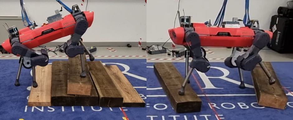
For this, we develop blind and perceptive control strategies for the ANYmal C quadruped and evaluate its performance for robust and dynamic locomotion over flat and uneven terrain as shown in Fig. 1.

I-A Related Work

Model-free data-driven deep reinforcement learning (RL) enables obtaining control solutions that have the potential to thoroughly utilize the system capabilities of current robots. This property has been leveraged for learning agile and dynamic robotic locomotion skills to perform blind bipedal traversal over stairs [16], quadrupedal locomotion over challenging terrains [17] and even robust quadrupedal state recovery [18]. Model-based techniques have also demonstrated dynamic and complex locomotion [19, 20, 21]. A combination of model-based and model-free methods have also been proposed [22, 23, 24, 25]. These approaches, however, often employ finite-order motion parameterization which inhibits the discovery of optimal behaviors. In contrast, motions executed by RL policies that map robot state information to desired joint states are not constrained by motion primitives. This makes RL particularly suitable for our task of obtaining motion control policies operating at frequencies as low as $5\text{\,}\mathrm{Hz}$. In such a case, the optimal behavior is not bounded by carefully tuned model-based controllers. Instead, the objective of finding the appropriate style to achieve dynamic and stable locomotion is addressed by the RL agent.

Despite the significant progress in RL for robotic locomotion, there remains an inconsistency in the design motivations for much of the proposed control architectures. In [26], Hwangbo et al. train an RL locomotion policy to map robot states to desired joint positions. This policy is queried at $200\text{\,}\mathrm{Hz}$ and the authors especially note that introducing a history of joint states into the RL state space is essential to obtain a locomotion policy. Rudin et al., however, train a locomotion policy at $50\text{\,}\mathrm{Hz}$ without utilizing joint state history [27]. The obtained policy is transferable to the real platform even with access to only the current proprioceptive state. In [28], Duan et al. also show bipedal locomotion at $40\text{\,}\mathrm{Hz}$ without utilizing joint state history. We study these differences and observe that at higher motion control frequencies, the controller is more sensitive to the actuation dynamics compared to at lower-frequencies. In the context of this work, low-frequency refers to $25\text{\,}\mathrm{Hz}$ or less. For a swing and stance phase duration of approximately $600\text{\,}\mathrm{ms}$ during locomotion, this corresponds to 15 or less control set points generated during each of these phases. We also observed that at less than $5\text{\,}\mathrm{Hz}$, corresponding to less than 3 set points generated during swing phase, the controller is unable to maintain stability during locomotion. We detail upon our findings in Section IV of this manuscript.

It is also worth mentioning that a rich body of work focuses on bio-inspired mechanical designs [29, 30, 31]. Although this is beyond the scope of our current work, we believe it serves as an important reminder that control intelligence and mechanical design complement each other [32].

I-B Contribution

Our main contribution with this work is presenting that low-frequency motion control is sufficient to perform robust and dynamic locomotion. We further show that dynamics randomization or actuation modeling may not even be necessary for successful sim-to-real transfer. We additionally provide a comparative analysis of motion control policies trained and deployed at a range of frequencies. We believe this work will provide an important reference to the robotic control research community with regards to design motivations for developing custom control solutions.

We additionally highlight our contributions relating to sharing of training and deployment code, the low-frequency motion control (LFMC) framework. We provide a RaiSim [33] based optimized implementation for training locomotion policies for ANYmal C at various motion control frequencies. This allows users to train policies in less than thirty minutes on a standard computer without requiring expensive hardware for massive parallelization [27]. We additionally provide minimal deployment code in both C++ and Python. For the Python version, we also provide an option to choose between the RaiSim and PyBullet [34] simulation engines. We hope this encourages reproducibility and allows colleagues to easily perform benchmarking against our approach.

II Preliminaries

II-A System Model

We model a quadrupedal robot as a floating base $B$ with four attached limbs. The robot state is measured and expressed in a global reference frame where the position is written as $\mathbf{r}_{B}\in\mathbb{R}^{3}$. The orientation is represented as the rotation matrix $\mathbf{R}_{B}\in\mathit{SO}(3)$. Each limb comprises three rotational joints. The angular joint positions are denoted by the vector $\mathbf{q}_{j}\in\mathbb{R}^{12}$. The linear and angular base velocities are represented as $\mathbf{v}_{B}\in\mathbb{R}^{3}$ and $\mathbf{\omega}_{B}\in\mathbb{R}^{3}$ respectively.

The joint control torques $\bm{\tau}_{j}\in\mathbb{R}^{12}$ actuate the quadrupedal system and are computed using the impedance control model,

$$\bm{\tau}_{j}=k_{p}\Delta\mathbf{q}_{j}-k_{d}\mathbf{\dot{q}}_{j}.$$ (1)

Here, $k_{p}$ and $k_{d}$ represent tracking gains and $\Delta\mathbf{q}_{j}=\mathbf{q}^{\ast}_{j}-\mathbf{q}_{j}$ where $\mathbf{q}^{\ast}_{j}$ denotes the desired joint positions.

II-B Control Architecture

Figure 2: Control architecture of our proprioceptive locomotion framework comprising a motion controller and an actuation tracker.

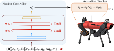
Our control architecture comprises a high-level motion controller and a low-level actuation tracker. This design is motivated by prior works on RL for robotic locomotion [26, 35, 36]. The motion controller, executed at a deployment frequency $f_{m}$, processes robot state information to generate desired joint states. The actuation tracker, executed at a frequency $f_{a}$ where $f_{a}\geq f_{m}$, tracks these desired joint states by generating $\bm{\tau}_{j}$ using the model described in Eq. 1.

We model the motion controller policy as a multi-layer perceptron (MLP), $\pi_{\theta}$. Here, $\theta$ represents the network parameters. The policy, $\pi_{\theta}:\mathbf{s}\mapsto\mathbf{a}$, maps the input state tuple $\mathbf{s}$ to actions $\mathbf{a}\in\mathbb{R}^{12}$. The tuple $\mathbf{s}$ comprises observations that can be accessed on the real robot. Since we perform comparative analysis of different types of policies, the dimensionality of $\mathbf{s}$ depends on the individual motion control policy. We discuss this in the following subsection.

Each of the policies outputs an action tuple, $\mathbf{a}:=\langle\mathbf{q}^{\ast}_{j}\rangle$, representing the desired joint positions and is based on the motivation that low-impedance joint position control can offer improved training and control performance over torque control [37].

II-C Motion Control Policies

We represent the motion control policies as $\pi_{\theta}$ where $\theta$ denotes the parameters of a generic motion controller. To refer to specific policies, we introduce the notation

$$\pi^{f_{t}}_{M:H}$$

where $f_{t}$ is the motion control frequency at which the policy was trained, $M$ is the mode of operation which can either be $b$ (for blind) or $p$ (for perceptive), and $H\in\mathbb{R}$ represents history length of joint states introduced in the state tuple $\mathbf{s}$. The joint state history is recorded at a frequency of $f_{j}$ with a corresponding time step $t_{j}$. In this work, the joint state recording frequency $f_{j}\geq{}f_{m}$. We use $f_{j}=$200\text{\,}\mathrm{Hz}$$ which we obtained empirically as part of [24].

As an example, $\pi^{8}_{b:2}$ represents a blind motion control policy trained at $8\text{\,}\mathrm{Hz}$. The state space of $\pi^{8}_{b:2}$ also contains $\mathbf{q}_{j}$ and $\mathbf{\dot{q}}_{j}$ at joint recording steps $t_{j}-1$ and $t_{j}-2$, corresponding to a history length of 2.

For brevity, we omit $f_{t}$ while referring to a class of motion control policies with the same operation mode and history length. For blind policies, $\pi_{b:0}$, with no joint state history, the state tuple $\mathbf{s}_{b:0}\in\mathbb{R}^{48}$ is defined as

$$\mathbf{s}_{b:0}:=\langle\mathbf{R}_{B}^{T}\mathbf{e}_{z},\mathbf{q}_{j},\mathbf{R}_{B}^{T}\mathbf{v}_{B},\mathbf{R}_{B}^{T}\mathbf{\omega}_{B},\mathbf{\dot{q}}_{j},\Delta\mathbf{q}_{j},\mathbf{c}^{\ast}\rangle,$$

where $\mathbf{e}_{z}=[0,0,1]^{T}$ represents the vertical $z$-axis and $\mathbf{c}^{\ast}\in\mathbb{R}^{3}$ comprises the desired heading velocity, lateral velocity and yaw rate commands represented in the base frame. The objective of the motion control policies is thus to track user-generated desired velocity commands.

The state space of perceptive policies $\pi_{p:0}$ is written as $\mathbf{s}_{p:0}\in\mathbb{R}^{235}$. $\mathbf{s}_{p:0}$ augments $\mathbf{s}_{b:0}$ with robo-centric terrain information $\mathbf{T}\in\mathbb{R}^{17\times{}11}$ observed between $[-0.8,0.8]\,$\mathrm{m}$$ along the heading axis and $[-0.5,0.5]\,$\mathrm{m}$$ along the lateral axis with a resolution of $0.1\text{\,}\mathrm{m}$. The perceptive state space design is based on [27].

The joint state history augments the state space dimensionality by $H\times 24$. For a blind policy with history length of 4, $\pi_{b:4}$, its state tuple $\mathbf{s}_{b:4}\in\mathbb{R}^{144}$ is written as

$$\mathbf{s}_{b:4}:=\langle\mathbf{s}_{b:0},\mathbf{q}_{t_{j}-1},\mathbf{q}_{t_{j}-2},\mathbf{q}_{t_{j}-3},\mathbf{q}_{t_{j}-4}\rangle.$$

Here, $\mathbf{q}_{t_{j}}$ represents the joint state tuple comprising joint positions and joint velocities recorded at time step $t_{j}$. The control architecture, including the dense neural network policy architecture, is illustrated in Fig. 2.

III Methodology

III-A Training

We represent our problem as a sequential Markov decision process (MDP) [38] with the goal of obtaining a policy, or a class of policies, that maximizes the expected cumulative discounted return,

$$J\left(\pi\right)\doteq\underset{\mathcal{T}\sim\pi_{\theta}}{\text{{E}}}\left[\sum_{t=0}^{N}{{\gamma}^{t}R}\right]\text{,}$$ (2)

where $\gamma\in\left[0,1\right)$ represents the discount factor and $\mathcal{T}$, dependent on $\pi_{\theta}$, denotes a finite-horizon trajectory with episode length $N$. Our reward function, $R$, comprises several reward terms that allow for efficient and stable tracking of reference base velocity commands. We use the proximal policy optimization (PPO) [39] strategy to train each of our policies. Our training approach, including the reward function, has been derived from prior works [26, 35, 27].

While our method is quite standard, training several policies for different motion control frequencies requires tuning of individual reward terms and hyperparameters such as $\gamma$. For example, for an episodic length of $1\text{\,}\mathrm{s}$, executing a policy at $200\text{\,}\mathrm{Hz}$ would imply collection of forty times more samples than for a $5\text{\,}\mathrm{Hz}$ policy. Additionally, the half-life of $\gamma$ can be given by,

$$n_{\gamma_{0.5}}=\frac{\log{}{0.5}}{\log{}\gamma}\approx\frac{-0.3}{\log{}\gamma}.$$ (3)

For $\gamma=0.98$, the half-life would correspond to 34 control steps. For a $200\text{\,}\mathrm{Hz}$ policy, this is equivalent to $0.17\text{\,}\mathrm{s}$ while for a $5\text{\,}\mathrm{Hz}$ policy, this represents a duration of $6.8\text{\,}\mathrm{s}$.

To ensure consistency across different training frequencies, we denote the duration of $n_{\gamma_{0.5}}$ in seconds as opposed to control steps. For a training frequency $f_{t}$, the discount factor can then be computed by

$$\gamma=exp\left(\frac{\log{}{0.5}}{f_{t}\times n_{\gamma_{0.5}}}\right).$$ (4)

In our training setup, we use $n_{\gamma_{0.5}}=$3\text{\,}\mathrm{s}$$. For an episodic length $N=$1\text{\,}\mathrm{s}$$, we ensure the batch size per policy iteration remains the same for every control frequency. For this, we perform parallel data collection wherein the number of parallel environments are scaled up to fit the desired batch size, $b_{s}=f_{t}\times{}n_{env}$. For $b_{s}=$48\text{\,}\mathrm{k}{}$$, we use $n_{env}=240$ for $f_{t}=$200\text{\,}\mathrm{Hz}$$, and $n_{env}=9600$ for $f_{t}=$5\text{\,}\mathrm{Hz}$$.

To avoid retuning the reward function, we compute and aggregate the returns at each simulation step, $t_{s}$ as opposed to each control step $t_{m}$. Normally, $t_{s}\leq t_{m}$ and we use $t_{s}=$0.0025\text{\,}\mathrm{s}$$ in this work. While this largely addresses exhaustive reward function tuning, we observed that reward terms representing deviation from nominal joint configuration and action smoothness needed to be slightly tuned for individual frequencies to achieve visually similar locomotion behavior. We provide the different training configurations on the project website.

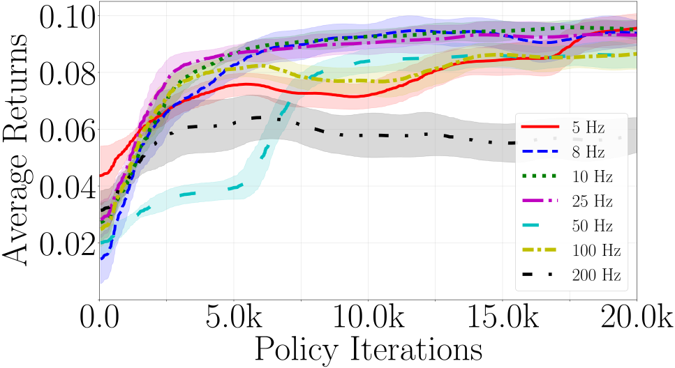
We train each of the $\pi_{b:0}$ policies for $20\text{\,}\mathrm{k}{}$ iterations. The iteration time is dependent on $f_{t}$ and varies between $0.4\text{\,}\mathrm{s}$ (for $f_{t}=$25\text{\,}\mathrm{Hz}$$ and $f_{t}=$50\text{\,}\mathrm{Hz}$$) to $1.5\text{\,}\mathrm{s}$ (for $f_{t}=$5\text{\,}\mathrm{Hz}$$ and $f_{t}=$200\text{\,}\mathrm{Hz}$$). on a standard desktop computer housing an 8-core $3.6\text{\,}\mathrm{GHz}$ Intel i9-9900K and an Nvidia RTX 2080Ti. The returns plot for each of the trained policies is shown in Fig. 3. The policies trained at low-frequencies ($8\text{\,}\mathrm{Hz}$, $10\text{\,}\mathrm{Hz}$ and $25\text{\,}\mathrm{Hz}$) converge a lot faster ($<$10k iterations) compared to high-frequency policies. Note, $\pi^{5}_{b:0}$ suffers from poor reactivity and is therefore harder to train.

Figure 3: Average returns for each of the trained policies $\pi_{b:0}$.

We do not perform any dynamics randomization (DR) while training the blind policies. Although we do use an actuator network [26] to model the real actuation dynamics, in Section IV, we show that introducing the actuator network during training may not even be necessary for LFMC.

III-B Evaluation

We follow the narrative of bio-inspired low-frequency motion control (LFMC) and discuss the following key observations and reasoning in Section IV.

• LFMC policies are less sensitive to actuation dynamics under the assumption that actuation settling time [40] is less than control step time (Section IV-A).

• LFMC policies do not perform implicit modeling of system dynamics necessary for predictive control at high frequencies. Instead, LFMC policies can operate as motion planners (Section IV-B). To support this, we visualize the policy network Jacobians in Fig. 7.

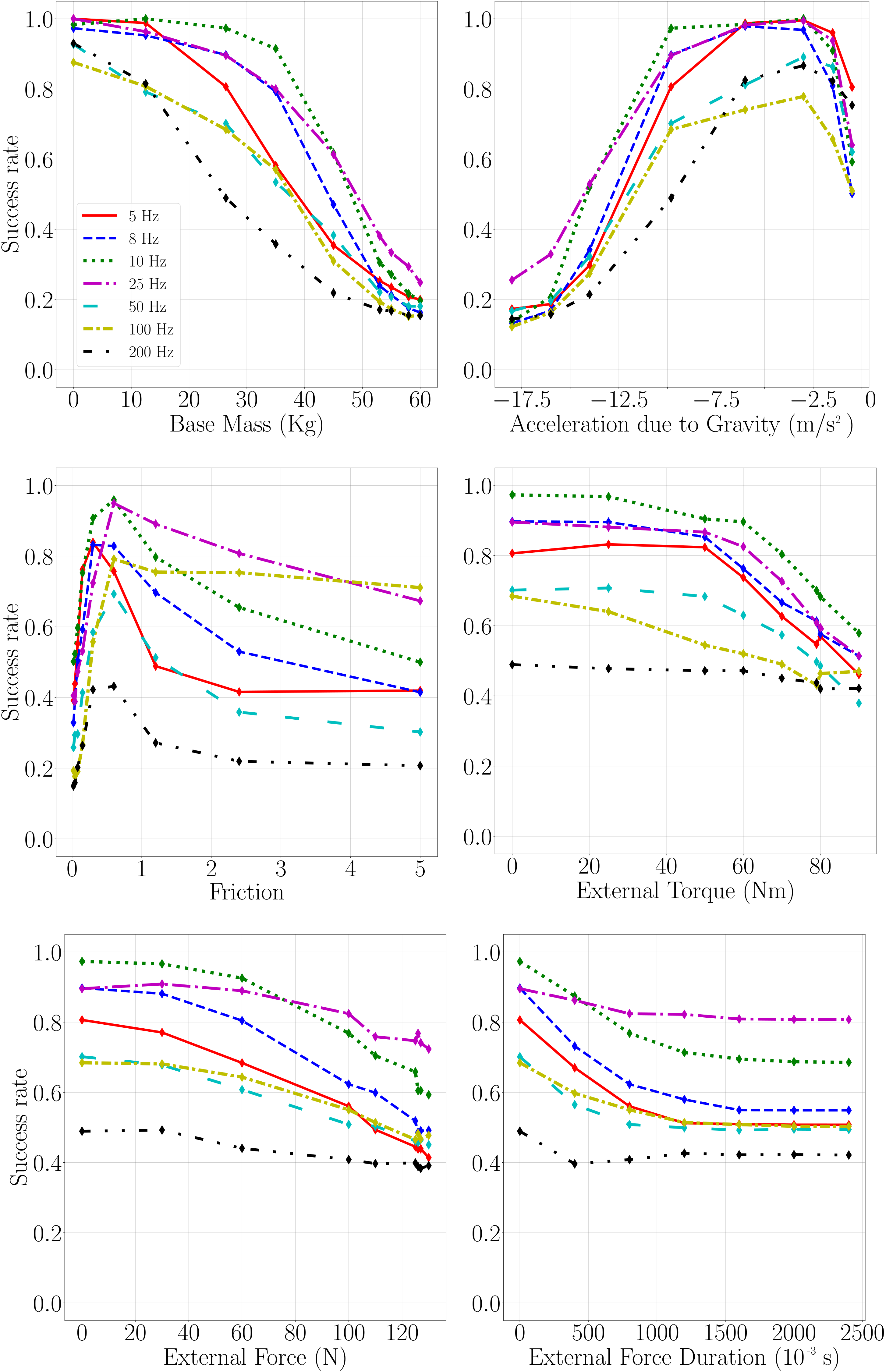
• Since LFMC policies operate as motion planners, they show more robustness to variations in system dynamics. This is based on the assumption that the low-level actuation tracker stably and reliably tracks the motion plans. We show this to be the case in Fig. 9.

• LFMC policies are faster to train (Fig. 3).

To support these points, we evaluate the performance of each of the individual blind $\pi_{b:0}$ policies in RaiSim with unstructured rough terrain generated using Perlin noise [41] with maximum extrusion of $0.15\text{\,}\mathrm{m}$. This is shown in Fig. 4. Our motivation for this setup is twofold: (1) the terrain noise introduces randomness allowing us to measure a probability distribution and (2) the unexpected perturbations highlight the reactivity of each of the policies.

We introduce success rate (SR) as a performance metric defined as,

$$\mathrm{SR}=1-\frac{N_{e}}{N_{T}}$$ (5)

where $N_{e}$ refers to the number of episodic rollouts that were terminated early due to an invalid robot state and $N_{T}$ represents the total number of rollouts. In this work, we use $N_{T}=100$. For each rollout, we randomize the base heading direction. This randomization occurs with the same seed across each of the policies. An invalid robot state is defined by the criteria: (1) $\arccos{(\mathbf{R}_{B_{3,3}})}>0.4\pi$ which relates to base orientation, (2) self-collisions, or (3) collision of the robot base with ground.

We train and compare $\pi^{10}_{b:4}$ and $\pi^{200}_{b:4}$ to show that joint state history is relevant for modeling system dynamics and is essential for high-frequency motion control as presented in [26]. This, however, is not the case for LFMC. We also evaluate the performance of perceptive locomotion policies on terrains comprising rough ground, stairs and bricks as shown in Fig. 4. Our evaluation method for perceptive locomotion policies is based on the setup introduced in [24].

Figure 4: RaiSim simulation set up for evaluation of blind and perceptive locomotion policies with ANYmal C traversing terrains comprising unstructured ground, stairs and bricks.

IV Results

This section presents the key results in support of our contribution. We provide an extended analysis on the project website. The project website also contains qualitative demonstrations of $8\text{\,}\mathrm{Hz}$ motion control in non-stationary environments such as unexpected slippery surfaces.

IV-A Intuitive Reasoning

Figure 5 (top) illustrates a toy example of a 1 DoF PD controller tracking sinusoidal set points updated at $5\text{\,}\mathrm{Hz}$ and $200\text{\,}\mathrm{Hz}$ for $k_{p}\in\{50,65,80,95\}$ and $k_{d}=2$. For the $5\text{\,}\mathrm{Hz}$ update frequency, the joint trajectories converge to very similar states before a new set point is generated. Note that, we use $k_{p}=80$ and $k_{d}=2.0$ for deploying our policies on to the real robot. For a $5\text{\,}\mathrm{Hz}$ controller, this implies the sensory readings at each update step are less effected by actuation tracking dynamics in comparison for higher update frequencies such as $200\text{\,}\mathrm{Hz}$. This implies that, for an effective control behavior, the $200\text{\,}\mathrm{Hz}$ policy requires observability of the actuation dynamics.

Figure 5: Top: Tracking of sinusoidal set points updated at $5\text{\,}\mathrm{Hz}$ and $200\text{\,}\mathrm{Hz}$ for various position tracking gains. Bottom: Step responses observed for $k_{p}\in\{60,100\}$ and $k_{d}\in\{0,2\}$ for a series elastic actuator present on the ANYmal C quadruped.

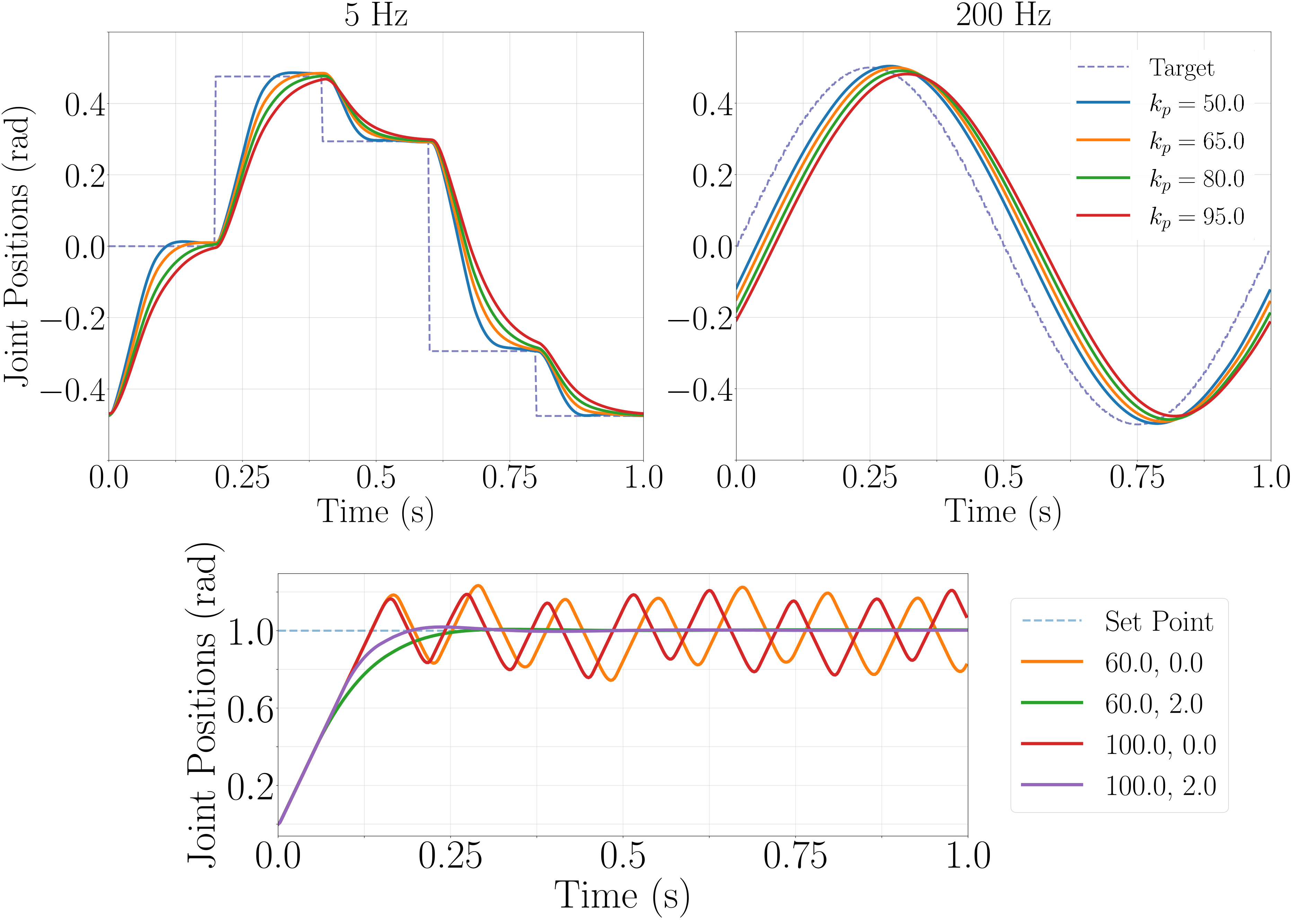
We hypothesize that LFMC allows for operation as a planner and refer to it as motion planning hypothesis. In this context, motion planning refers to generation of target states without an adaptive tracking system as is common in optimization-based approaches [2] which utilize a planner in addition to a whole-body controller. This makes low-frequency motion controllers robust to actuation dynamics under the assumption that the low-level actuation controller stably tracks the generated joint states. Figure 5 (bottom) illustrates why the stable tracking is necessary. For cases of under or over-damping, the motion controller may be required to adapt to the settling state even with low-frequency control.

Figure 6: Gait sequences for various $\pi_{b:0}$ motion control policies. The coloured regions represent stance phase.

Figure 7: Visualization of the mean of network Jacobians recorded for $\pi^{10}_{b:4}$ and $\pi^{200}_{b:4}$ for $2\text{\,}\mathrm{s}$. Dark blue regions correspond to high gradients whereas white corresponds to zero gradients. The brown regions separate different observations and have only been included for visual aid. Note that, joint state history is sampled at $200\text{\,}\mathrm{Hz}$ for both the policies. Sampling joint state history at $10\text{\,}\mathrm{Hz}$ for $\pi^{10}_{b:4}$ resulted in near-zero gradients for history terms.

Figure 8: Motion control policy trained and deployed at $8\text{\,}\mathrm{Hz}$ stably tracking heading base velocity of $1.5\text{\,}\mathrm{m}\text{\,}{\mathrm{s}}^{-1}$.

Figure 9: Success rate observed for various motion control policies, $\pi_{b:0}$, for different perturbations and dynamics parameters.

IV-B Qualitative and Behavioral Analysis

We test the motion planning hypothesis by transferring the trained motion control policies on to the real ANYmal C quadruped. We observe extremely aggressive actuation tracking for $\pi^{200}_{b:0}$ resulting in vibrations at the rotary joints. This aggressive behavior is reduced with lower-frequency policies and no vibrations are recorded for $\pi^{25}_{b:0}$ and lower. We suspect that, since no dynamics randomization (DR) was performed during training, and due to imperfect actuation modeling, high-frequency policies overfit to the simulation domain affecting sim-to-real transfer. Note, while we are able to transfer $\pi^{5}_{b:0}$ onto the real robot, we are only able to stably execute low-velocity motions. The $5\text{\,}\mathrm{Hz}$ policy suffers from poor reactivity and is unable to execute recovery actions in unstable states.

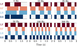
We observe interesting behavior with regards to the stance (foot-in-contact) and swing (foot-not-in-contact) phase duration. Low-frequency policies exhibit larger stance and swing phases compared to high-frequency policies (Fig. 6). We expected this to be an artifact of the scaling of action smoothness reward term (which penalizes large deviations between current and previous actions) with variations in motion control training frequencies. This, however, was not the case when we introduced joint state history ($N\geq 4$) into the state space. Hwangbo et al. hypothesized that the joint state history implicitly modeled contact detection [26]. While this has been consistent with our analysis of observing the absolute of policy Jacobians, $\absolutevalue{d\pi_{\theta}(s)/d{}s}$, as presented in [17], we also observed that high-frequency control policies are more dependent on joint state history than low-frequency policies. We posit that joint state history improves the domain observability through implicit encoding of actuation dynamics [42] and is therefore more relevant for high-frequency policies.

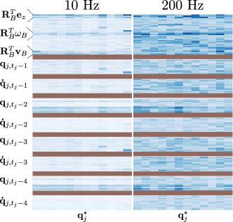
We further investigate this for $\pi^{10}_{b:4}$ and $\pi^{200}_{b:4}$. Figure 7 illustrates the mean of the policy Jacobians recorded for a duration of $2\text{\,}\mathrm{s}$. Dark blue regions suggest higher gradients, implying larger dependency. Compared to $10\text{\,}\mathrm{Hz}$, the $200\text{\,}\mathrm{Hz}$ policy requires more observations to execute the same task relating to larger dependency on system dynamics. Interestingly, the gradients for joint velocities are quite low for $\pi^{10}_{b:4}$ while $\pi^{200}_{b:4}$ utilizes joint velocities more than joint positions. The gradients observed along the base velocity states were also negligible for $10\text{\,}\mathrm{Hz}$ policy, compared to $200\text{\,}\mathrm{Hz}$, even during high-speed locomotion suggesting that LFMC policies do not considerably rely on base-velocity measurements.

For high-frequency $\pi_{b:0}$, we suspect the fast contact switching behavior occurs due to partial observability of the system dynamics. In our experience, we have observed this to be the case for poorly designed state spaces. This, however, needs further investigating. For the $200\text{\,}\mathrm{Hz}$ policy, the increase in stance and swing phase duration, compared to $100\text{\,}\mathrm{Hz}$ policy, is due to poor tracking with lower stability.

IV-C Robustness Analysis

One of our main objectives with this work is to demonstrate robustness with low-frequency motion control. Figure 9 shows that $\pi^{10}_{b:0}$ performs better than most of the policies. $\pi^{25}_{b:0}$ offers both high robustness and reactivity whereas $\pi^{8}_{b:0}$ falls behind $\pi^{10}_{b:0}$ due to inadequate reactivity for traversal over rough terrain. We also investigate robustness to actuation latencies and show that LFMC policies offer higher robustness than high-frequency policies (Table I).

TABLE I: Maximum actuation delay that $\pi_{b:0}$ policies can be robust to right before failure measured at a resolution of $5\text{\,}\mathrm{ms}$.

Training Frequency (Hz)	5	10	25	50	100	200
Latency (ms)	90	90	65	50	30	20

IV-D Dynamic Locomotion

We perform qualitative evaluation on the real robot and demonstrate high-speed dynamic locomotion with $\pi^{8}_{b:0}$. As shown in Fig. 8, we are able to achieve a heading velocity of approximately $1.5\text{\,}\mathrm{m}\text{\,}{\mathrm{s}}^{-1}$ traversing a distance of $2\text{\,}\mathrm{m}$ in roughly $1.33\text{\,}\mathrm{s}$.

We also train a perceptive locomotion policy $\pi^{8}_{p:0}$ based on [27]. We show that $8\text{\,}\mathrm{Hz}$ motion control is sufficient for robust traversal over considerable obstacles (wooden railway sleepers) and steps (both up and down) as presented in Fig. 1.

We further compare the behavior of policies trained with and without DR. The DR parameters are based on [35] and have been provided on the project website. This is shown for $10\text{\,}\mathrm{Hz}$ and $200\text{\,}\mathrm{Hz}$ perceptive policies in Table II. As expected, DR allows for better performance over uneven terrain. Introduction of joint state history is not as effective as doing both, introducing joint state history and DR. Joint state history and DR allow for better observability of environment interactions, necessary for uneven terrains [17], while also encouraging generalizability to unseen domains.

We are also able to demonstrate transfer on to the physical system with policies trained without the actuator network. The behavior is stable, however, not as smooth as policies trained with the actuator network. We detail upon the extended analysis on the project website and summarize our evaluation in the overview video.

TABLE II: Success rates of $10\text{\,}\mathrm{Hz}$ and $200\text{\,}\mathrm{Hz}$ perceptive policies measured for 100 runs each.

	$10\text{\,}\mathrm{Hz}$				$200\text{\,}\mathrm{Hz}$
	$\pi_{p:0}$	$\pi_{p:0}$ (DR)	$\pi_{p:4}$	$\pi_{p:4}$ (DR)	$\pi_{p:0}$	$\pi_{p:0}$ (DR)	$\pi_{p:4}$	$\pi_{p:4}$ (DR)
Rough	0.94	0.94	0.94	0.95	0.87	0.92	0.93	0.94
Stairs	0.86	0.93	0.92	0.94	0.52	0.59	0.88	0.95
Bricks	0.66	0.71	0.69	0.80	0.58	0.62	0.64	0.76

V Conclusion

This work aims to start the discussion within the robotics community about the role and benefit of high- versus low-frequency motion control, especially within the context of learning-based approaches. From biological studies we know that animals can perform robust and dynamic locomotion at low motion control frequencies and, with this work, we showed how real robots can achieve this too.

We demonstrated dynamic and robust quadrupedal locomotion with as low as $8\text{\,}\mathrm{Hz}$ of motion control frequency. We further provided empirical evaluations to support our claim that motion control policies trained at low-frequencies do not require dynamics randomization or actuation modeling to perform a successful sim-to-real transfer.

References

- [1] J. Di Carlo, P. M. Wensing, B. Katz, G. Bledt, and S. Kim, “Dynamic locomotion in the mit cheetah 3 through convex model-predictive control,” in 2018 IEEE/RSJ international conference on intelligent robots and systems (IROS). IEEE, 2018, pp. 1–9.
- [2] C. D. Bellicoso, F. Jenelten, C. Gehring, and M. Hutter, “Dynamic locomotion through online nonlinear motion optimization for quadrupedal robots,” IEEE Robotics and Automation Letters, vol. 3, no. 3, pp. 2261–2268, July 2018.
- [3] Y. Yang, T. Zhang, E. Coumans, J. Tan, and B. Boots, “Fast and efficient locomotion via learned gait transitions,” in Conference on Robot Learning. PMLR, 2022, pp. 773–783.
- [4] A. A. Faisal, L. P. Selen, and D. M. Wolpert, “Noise in the nervous system,” Nature reviews neuroscience, vol. 9, no. 4, pp. 292–303, 2008.
- [5] H. L. More, J. R. Hutchinson, D. F. Collins, D. J. Weber, S. K. Aung, and J. M. Donelan, “Scaling of sensorimotor control in terrestrial mammals,” Proceedings of the Royal Society B: Biological Sciences, vol. 277, no. 1700, pp. 3563–3568, 2010.
- [6] H. L. More, S. M. O’Connor, E. Brøndum, T. Wang, M. F. Bertelsen, C. Grøndahl, K. Kastberg, A. Hørlyck, J. Funder, and J. M. Donelan, “Sensorimotor responsiveness and resolution in the giraffe,” Journal of Experimental Biology, vol. 216, no. 6, pp. 1003–1011, 2013.
- [7] H. L. More and J. M. Donelan, “Scaling of sensorimotor delays in terrestrial mammals,” Proceedings of the Royal Society B, vol. 285, no. 1885, p. 20180613, 2018.
- [8] M. S. Ashtiani, A. Aghamaleki Sarvestani, and A. Badri-Spröwitz, “Hybrid parallel compliance allows robots to operate with sensorimotor delays and low control frequencies,” Frontiers in Robotics and AI, p. 170, 2021.
- [9] J. E. Bertram, A. Gutmann, J. Randev, and M. Hulliger, “Domestic cat walking parallels human constrained optimization: optimization strategies and the comparison of normal and sensory deficient individuals,” Human Movement Science, vol. 36, pp. 154–166, 2014.
- [10] R. Blickhan, A. Seyfarth, H. Geyer, S. Grimmer, H. Wagner, and M. Günther, “Intelligence by mechanics,” Philosophical Transactions of the Royal Society A: Mathematical, Physical and Engineering Sciences, vol. 365, no. 1850, pp. 199–220, 2007.
- [11] E. Ackerman, “Anybotics introduces sleek new anymal c quadruped,” IEEE Spectrum. https://spectrum.ieee.org/automaton/robotics/industrial-robots/anybotics-introduces-sleek-new-anymal-c-quadruped, 2019.
- [12] G. A. Pratt and M. M. Williamson, “Series elastic actuators,” in Proceedings 1995 IEEE/RSJ International Conference on Intelligent Robots and Systems. Human Robot Interaction and Cooperative Robots, vol. 1. IEEE, 1995, pp. 399–406.
- [13] G. Bledt, M. J. Powell, B. Katz, J. Di Carlo, P. M. Wensing, and S. Kim, “Mit cheetah 3: Design and control of a robust, dynamic quadruped robot,” in 2018 IEEE/RSJ International Conference on Intelligent Robots and Systems (IROS). IEEE, 2018, pp. 2245–2252.
- [14] G. Ji, J. Mun, H. Kim, and J. Hwangbo, “Concurrent training of a control policy and a state estimator for dynamic and robust legged locomotion,” IEEE Robotics and Automation Letters, vol. 7, no. 2, pp. 4630–4637, 2022.
- [15] T. Miki, J. Lee, J. Hwangbo, L. Wellhausen, V. Koltun, and M. Hutter, “Learning robust perceptive locomotion for quadrupedal robots in the wild,” Science Robotics, vol. 7, no. 62, p. eabk2822, 2022.
- [16] J. Siekmann, K. Green, J. Warila, A. Fern, and J. Hurst, “Blind bipedal stair traversal via sim-to-real reinforcement learning,” arXiv preprint arXiv:2105.08328, 2021.
- [17] J. Lee, J. Hwangbo, L. Wellhausen, V. Koltun, and M. Hutter, “Learning quadrupedal locomotion over challenging terrain,” Science Robotics, vol. 5, no. 47, 2020. [Online]. Available: https://robotics.sciencemag.org/content/5/47/eabc5986
- [18] C. Yang, K. Yuan, Q. Zhu, W. Yu, and Z. Li, “Multi-expert learning of adaptive legged locomotion,” Science Robotics, vol. 5, no. 49, p. eabb2174, 2020.
- [19] R. Grandia, F. Farshidian, R. Ranftl, and M. Hutter, “Feedback mpc for torque-controlled legged robots,” in 2019 IEEE/RSJ International Conference on Intelligent Robots and Systems (IROS), 2019, pp. 4730–4737.
- [20] F. Jenelten, T. Miki, A. E. Vijayan, M. Bjelonic, and M. Hutter, “Perceptive locomotion in rough terrain–online foothold optimization,” IEEE Robotics and Automation Letters, vol. 5, no. 4, pp. 5370–5376, 2020.
- [21] D. Kim, D. Carballo, J. Di Carlo, B. Katz, G. Bledt, B. Lim, and S. Kim, “Vision aided dynamic exploration of unstructured terrain with a small-scale quadruped robot,” in 2020 IEEE International Conference on Robotics and Automation (ICRA). IEEE, 2020, pp. 2464–2470.
- [22] T. Zhang, G. Kahn, S. Levine, and P. Abbeel, “Learning deep control policies for autonomous aerial vehicles with mpc-guided policy search,” in 2016 IEEE international conference on robotics and automation (ICRA). IEEE, 2016, pp. 528–535.
- [23] Z. Xie, G. Berseth, P. Clary, J. W. Hurst, and M. van de Panne, “Feedback control for cassie with deep reinforcement learning,” CoRR, vol. abs/1803.05580, 2018. [Online]. Available: http://arxiv.org/abs/1803.05580
- [24] S. Gangapurwala, M. Geisert, R. Orsolino, M. Fallon, and I. Havoutis, “Rloc: Terrain-aware legged locomotion using reinforcement learning and optimal control,” 2020.
- [25] ——, “Real-time trajectory adaptation for quadrupedal locomotion using deep reinforcement learning,” in Proceedings of the International Conference on Robotics and Automation (ICRA). Institute of Electrical and Electronics Engineers, 2021.
- [26] J. Hwangbo, J. Lee, A. Dosovitskiy, D. Bellicoso, V. Tsounis, V. Koltun, and M. Hutter, “Learning agile and dynamic motor skills for legged robots,” Science Robotics, vol. 4, no. 26, p. eaau5872, 2019.
- [27] N. Rudin, D. Hoeller, P. Reist, and M. Hutter, “Learning to walk in minutes using massively parallel deep reinforcement learning,” in Conference on Robot Learning. PMLR, 2022, pp. 91–100.
- [28] H. Duan, J. Dao, K. Green, T. Apgar, A. Fern, and J. Hurst, “Learning task space actions for bipedal locomotion,” in 2021 IEEE International Conference on Robotics and Automation (ICRA). IEEE, 2021, pp. 1276–1282.
- [29] A. A. Saputra, N. Takesue, K. Wada, A. J. Ijspeert, and N. Kubota, “Aquro: A cat-like adaptive quadruped robot with novel bio-inspired capabilities,” Frontiers in Robotics and AI, vol. 8, p. 562524, 2021.
- [30] A. J. Ijspeert, “Central pattern generators for locomotion control in animals and robots: a review,” Neural networks, vol. 21, no. 4, pp. 642–653, 2008.
- [31] S. Coyle, C. Majidi, P. LeDuc, and K. J. Hsia, “Bio-inspired soft robotics: Material selection, actuation, and design,” Extreme Mechanics Letters, vol. 22, pp. 51–59, 2018.
- [32] R. Pfeifer, M. Lungarella, and F. Iida, “The challenges ahead for bio-inspired’soft’robotics,” Communications of the ACM, vol. 55, no. 11, pp. 76–87, 2012.
- [33] J. Hwangbo, J. Lee, and M. Hutter, “Per-contact iteration method for solving contact dynamics,” IEEE Robotics and Automation Letters, vol. 3, no. 2, pp. 895–902, 2018.
- [34] E. Coumans and Y. Bai, “Pybullet, a python module for physics simulation for games, robotics and machine learning,” http://pybullet.org, 2016–2021.
- [35] S. Gangapurwala, A. Mitchell, and I. Havoutis, “Guided constrained policy optimization for dynamic quadrupedal robot locomotion,” IEEE Robotics and Automation Letters, vol. 5, no. 2, pp. 3642–3649, 2020.
- [36] Z. Xie, X. Da, M. van de Panne, B. Babich, and A. Garg, “Dynamics randomization revisited: A case study for quadrupedal locomotion,” in 2021 IEEE International Conference on Robotics and Automation (ICRA). IEEE, 2021, pp. 4955–4961.
- [37] X. B. Peng and M. van de Panne, “Learning locomotion skills using deeprl: Does the choice of action space matter?” in Proceedings of the ACM SIGGRAPH/Eurographics Symposium on Computer Animation, 2017, pp. 1–13.
- [38] R. S. Sutton, A. G. Barto, et al., Introduction to reinforcement learning. MIT press Cambridge, 1998, vol. 135.
- [39] J. Schulman, F. Wolski, P. Dhariwal, A. Radford, and O. Klimov, “Proximal policy optimization algorithms,” 2017.
- [40] S. N. Vukosavic, Electrical machines. Springer Science & Business Media, 2012.
- [41] K. Perlin, “Improving noise,” in Proceedings of the 29th annual conference on Computer graphics and interactive techniques, 2002, pp. 681–682.
- [42] I. Akkaya, M. Andrychowicz, M. Chociej, M. Litwin, B. McGrew, A. Petron, A. Paino, M. Plappert, G. Powell, R. Ribas, et al., “Solving rubik’s cube with a robot hand,” arXiv preprint arXiv:1910.07113, 2019.