A case study of spatiotemporal forecasting techniques for weather forecasting

Abstract

The majority of real-world processes are spatiotemporal, and the data generated by them exhibits both spatial and temporal evolution. Weather is one of the most important processes that fall under this domain, and forecasting it has become a crucial part of our daily routine. Weather data analysis is considered the most complex and challenging task. Although numerical weather prediction models are currently state-of-the-art, they are resource intensive and time-consuming. Numerous studies have proposed time-series-based models as a viable alternative to numerical forecasts. Recent research has primarily focused on forecasting weather at a specific location. Therefore, models can only capture temporal correlations. This self-contained paper explores various methods for regional data-driven weather forecasting, i.e., forecasting over multiple latitude-longitude points to capture spatiotemporal correlations. The results showed that spatiotemporal prediction models reduced computational cost while improving accuracy; in particular, the proposed tensor train dynamic mode decomposition-based forecasting model has comparable accuracy to ConvLSTM without the need for training. We use the NASA POWER meteorological dataset to evaluate the models and compare them with the current state of the art.

[inst1]organization=CAIT, Skolkovo institute of science and technology,addressline=Bolshoy Bulvar, city=skolkovo, postcode=121205, state=Moscow, country=Russia

1 Introduction

Time series forecasting has played a vital role in a range of real-world applications, including financial investments, traffic forecasting, supply chain management, epidemiology, and health monitoring. Weather forecasting is one of the essential applications of time-series analysis, which has been the most appealing research area in statistical physics, data assimilation, data science, etc. We all know that the sky can be clear one moment and cloudy, rainy, or completely different the very next. The chaotic nature of the weather makes weather forecasting extremely challenging. Weather forecasting deals with temperature, vapour pressure, precipitation, humidity, irradiance, wind speeds, and other variables. Precise forecasting of these variables is crucial for maintaining safety and helps us mitigate the hazardous effects of upcoming natural disasters, including floods, storms, tornadoes, and many others. An accurate weather forecast is also crucial to many businesses and industries, such as agriculture and mining, as well as tourism and food processing, sports, naval systems, and airports. In the agriculture sector, for example, prior knowledge of these variables will assist farmers in taking the necessary actions to improve crop yield. We need prior knowledge of wind speed and rainfall to make the proper control parameter settings to maximize energy harvesting from wind and hydroelectric turbines. Solar irradiation, which varies depending on location, is critical for solar PV projects, as shown in [1].

Until the 1950s, weather predictions were primarily based on weather charts. Meteorologists regularly prepared synoptic weather maps to predict the average climate dynamics after observing these charts. In 1922 [2], the author proposed a numerical model for weather prediction by formulating a set differential equation for meteorological variables; however, the results presented were poor due to the author’s manual solution of the system equations. The basic idea behind numerical weather prediction (NWP) is to solve a set of nonlinear PDEs (also known as primitive equations) over the different grid points in latitude and longitude space with known initial conditions. Finally, the solutions of the system equations govern the atmospheric evolution [3]. The first successful NWP with barotropic vorticity equations was done in [4]. In [5], authors presented different aspects for better and simplified forecasting by solving approximated equations. The approximate models reduced computation costs and enabled researchers to have more control over model resolution. However, there are several issues with numerical weather prediction models, some of which are related to the physics of meteorological variables and some of which are technical. One fundamental issue with NWP is the uncertainty associated with initial conditions; we know that accurate initial conditions are essential for evolving nonlinear chaotic system states; otherwise, the solution trajectory will be completely different, a phenomenon known as the butterfly effect. Many researchers have incorporated newly observed data and compared it to previous forecasts in order to update model states in such a way that the forecast trajectory remains close to true measurements; this approach is known as data assimilation, and it has been very successful in weather forecasting [5], [6]. Computational resources and computation time are two other significant issues with NWP models. Models with high spatial and temporal resolution require a lot of computing power, and current implementation methods take long model run times [7]. With these issues in mind and the enormous success of data-driven approaches, researchers are now focusing on data-driven weather forecasting methods. Some researchers use data-driven approaches for preprocessing and postprocessing, while others have focused exclusively on data-driven techniques for weather forecasting.

Weather data is typically spatiotemporal, meaning it is collected across the space and time axes. Given that the climate phenomenon results from the interaction of spatial and temporal dynamic patterns, we examine what happens at a particular location and time. Researchers have mainly focused on using location-specific time-series-based models for weather forecasts. Therefore, models can only capture temporal correlations since they do not have a spatial component in modelling, which is essential for spatiotemporal processes. This paper explores regional data-driven weather forecasting, i.e., forecasting over multiple latitude-longitude points to capture spatiotemporal correlations. Weather forecasting is assumed to be extremely difficult and even theoretically impossible. Therefore, this work aims to determine the extent to which existing methodologies can produce meaningful forecasts. More specifically, the paper provides a stand-alone spatiotemporal forecasting background and methodologies, including the following major contributions:

• We set out to investigate the idea of including spatiotemporal correlations in different models.

• We populate the idea by presenting two spatiotemporal modelling approaches (sampling and clustering) based on dimensionality reduction, in which we identify important locations/subregions on the earth’s surface using haversine distance-based clustering, train models on centered locations, and use these models to make forecasts at each location within their respective clusters. These two models have significantly decreased the computation compared to the naive strategy, which is to train separate models on each latitude-longitude grid point.

• We adapt tensor-based dynamic mode decomposition (DMD) for spatiotemporal forecasting; the proposed methodology extends the classical DMD forecasting approach to predict 2D matrices rather than vectors. We evaluated the model on the NASA POWER weather dataset and compared it to state-of-the-art models.

Let’s highlight a few of the important notations used in this work before moving on to the next section.

Notations

$x,\mathbf{x},\mathbf{X}$	scalar, vector, and matrix
$\underline{\mathbf{X}}\in\mathbb{R}^{n_{1}\times\cdots\times n_{d}}$	$d^{\small th}$order tensor with $n_{l}$ denoting
	the size of the $l$th mode
$x_{i_{1},i_{2},\cdots i_{d}}=\underline{\mathbf{X}}_{i_{1},\ldots,i_{d}}$	A particular entry of $d^{\small th}$ order tensor
$\mathbf{X^{\top}},\mathbf{X^{-1}},\mathbf{X^{\dagger}}$	transpose, inverse, and pseudo-inverse
	of a matrix $\mathbf{X}$
$\odot,\otimes$	Khatri–Rao, Kronecker products
vec$(\mathbf{X})$, vec$(\underline{\mathbf{X}})$	vectorization of $\mathbf{X}$ or $\underline{\mathbf{X}}$
$\underline{\mathbf{A}}^{(l)},~{}\underline{\mathbf{X}}^{(l)},~{}\underline{\mathbf{Y}}^{(l)}$	core tensors

The rest of the paper is organised as follows: The section 2 below describes the current state of the art in time series and spatiotemporal weather forecasting. Section 3 discusses various types of spatiotemporal weather forecasting models. The experimental results are presented in the section 4. The last section discusses the conclusion and future extensions.

2 Related work

2.1 Time series forecasting

Data-driven forecasting models use past states to predict the future states. Mathematically, we can write :

$$\hat{\mathbf{x}}_{t+1},\hat{\mathbf{x}}_{t+2},\cdots,\hat{\mathbf{x}}_{t+h}=\mathbf{f}\left(\mathbf{x}_{t-T+1},\cdots,\mathbf{x}_{t-1},\mathbf{x}_{t}\right),$$ (1)

where $\mathbf{f}$ is function that takes set of past states and predicts $h$ future states. One of the simplest methods is the naive time series model, which sets the prediction state as the most recent state in the past. Another basic idea is to predict the future by linearly regressing a set of previous states; this method is known as autoregression. Another similar method is the moving average model, which predicts the arithmetic mean of the most recent past states. Jenkins and Box proposed a statistical model based on past sequences, the most famous being the auto-regressive integrated moving average (ARIMA). This model combined the features of both auto-regression and moving average [8]. ARIMA was used by researchers in [9], for monthly rainfall forecasting and synthetic generation. They tested ARIMA(1,1) and found it the best model for forecasting and synthetic generation of rainfall time series, passing the goodness-of-fit test in every case. They also investigated seasonally differenced and multiplicative models and applied them to the square-root of time series, concluding that differenced models are only useful for forecasting and cannot be used for a synthetic generation because the monthly standard deviation of time series is lost. Researchers in [10], have used singular spectrum analysis to decompose the annual run-off time-series into simple sub-series, and then used ARIMA on each simple sub-time series. Finally, they combine these individual forecasts using a correlation procedure. They compared this hybrid model to a variety of other models and found that the hybrid model outperformed them by a good margin. In [11], authors used time-series data of monthly mean temperature from an automatic weather station located at lat=118°54’, lon=31°56’, with the training data spanning 1951 to 2014 and the test data spanning 2015 to 2017. They have used the SARIMA model with different parameters to forecast on a normalized dataset. The accuracy of the model was validated by a diagnosis check, and they concluded that the MSE was quite low, with an increasing trend of 0.05/year.

The current success of AI-driven algorithms and their applicability for approximating any complex functions [12], [13]. In [14], researchers used the support vector machine (SVM) [15] and the extreme gradient boosting (XGB) proposed in [16], to estimate global solar radiation. XGB and SVM performed very well in terms of accuracy and stability when compared with known empirical models [17], [18]. They claimed that XGB has comparable forecast accuracy while also being more stable. In [19], the authors found a helpful way of using neural networks to model and forecast trends in time series data. The researchers in [20], compared the ANN models to forecast daily flows at multiple gauging stations. Several neural network architectures have been proposed for time series prediction in the last decade. Because of their promising results for forecasting tasks, some researchers are also developing hybrid models, such as [21], in which the researchers combine wavelet analysis with NN.

2.2 Spatio-temporal sequence forecasting

In the above section, we discussed the models for forecasting univariate or multivariate time series at a specific location. This section will review the literature on spatiotemporal sequences, i.e., datasets that vary in time and space.

Spatiotemporal sequence forecasting (STSF) is similar to the time series prediction problem shown in equation 1, except that instead of simple vectors at each time instant, we now have matrices or higher-order tensors. For example, video is a spatiotemporal series with dimensions of $H\times W\times T$, where $H$ denotes frame height, $W$ denotes frame width, and $T$ denotes sequence length. At each time instance, we have a frame of size $H\times W$. Researchers in [22], and [23] classified spatiotemporal datasets broadly into three categories based on their spatial and temporal coordinates. In the first case, both the space and time coordinates are fixed, but the dataset contains distinct events with associated location and time stamps; the data does not exhibit temporal or spatial evolution. In the second case, we have a fixed space (locations), but the values of measurements change along the temporal axis, as illustrated in Figure 2, the regional weather dataset and the video data are real-world examples. Moreover, the dataset used in this paper falls into this category. In the final category, both spatial and temporal coordinates change; GPS tracking is a classic example, as illustrated in Figure 2.

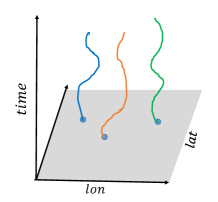
Figure 1: Locations are fixed, measurement values vary over time axis.

Figure 2: Measurement values change over location and time coordinates.

Researchers in [24] have shown how to use spatial information in autoregressive models, the so-called spatiotemporal autoregressive model (STAR). The idea of the STAR model is to include the neighbouring effects in the classical autoregressive model by explicitly modelling spatial and temporal dependencies. The authors of [25] used STAR on the Fairfax housing dataset, which is evolving in both time and space dimensions. The authors claimed that the spatiotemporal autoregressive model reduced median absolute error by 37.35% as compared to the indicator-based model. In [25], the authors propose a spatiotemporal precipitation model, which they evaluate on three-hourly Swiss rainfall data collected from 26 stations. These models are sometimes referred to as feature-based models due to the fact that they require human-engineered spatiotemporal features [23]. The major downside of these models is that their performance is highly dependent on these designed features and is not feasible when data size increases.

Machine learning and deep learning models are also now being used to forecast spatiotemporal sequences. Spatiotemporal prediction models are typically developed by combining convolutional neural networks (CNNs) (to account for spatial features, [26]) and recurrent neural networks (to account for temporal evolution [27]). Researchers have proposed a combined convolutional neural network and long short-term memory (LSTM) prediction scheme for the Urban PM2.5 Concentration (air pollution) dataset in [28]. They used a convolutional layer as the base layer for extracting features from massive environmental data and the LSTM at the output layer to account for temporal ordering. They compared the proposed model’s performance to that of numerical models and concluded that combining convolution and LSTM results in superior performance. The main breakthrough model, which was a modification of the classical LSTM, used convolution operations inside the LSTM model to include spatial features [29]. They conducted experiments on radar echo datasets for precipitation nowcasting and found that ConvLSTM outperformed FC-LSTM and the state-of-the-art Real-time Optical flow by Variational methods for Echoes of Radar (ROVER) algorithm [30]. In [31], researchers presented the spatiotemporal convolution sequence network, which uses only convolution layers for spatial and temporal modelling. The main downside of conventional CNN is that it cannot respect the temporal ordering and cannot produce an output sequence length greater than the input sequence length [32], so it hinders to forecast several steps as per needed. The authors in [31] have mainly solved these two difficulties by developing a model solely utilizing convolution layers. Basically, they split the 3D convolution operation (kernel decomposition) into two blocks: temporal and spatial. The temporal block is used to learn temporal correlation, while the spatial block is used to learn spatial features. The temporal generation block handles the causality requirement and generates output sequences that are longer than the input sequences. Only spatial representations are extracted by the spatial block; for details, please see [31], [33]. Most of the deep learning models we described above consider spatiotemporal sequence forecasting as a video prediction problem, i.e., the model takes input a set of $l$ frames and outputs the future $h$ frames, where $l$ is lookback, and $h$ is the forecast horizon.

3 Spatiotemporal weather forecasting models

Weather time series are collected across various latitude and longitude points and fall into the category where we have fixed spatial coordinates and the measurements change over time, as shown in Figure 2. There are many ways to make predictions in this situation. One of the most straightforward ideas for forecasting time series at multiple locations is to use location-specific models to forecast at each location separately. This method has two major flaws: first, it is computationally expensive and requires a large amount of memory to save separate models, limiting its applicability to small areas; second, it ignores the effects of neighbouring time series. In general, this approach is not feasible. Instead of training models at each individual location, one may select a subset of locations to train the models and then test/evaluate them at all locations, with each trained model being tested in its neighbourhood. The main issue now is how to sample these points in the region. One of the simplest methods is naive sampling, which randomly draws a desired number of points from latitude-longitude space. However, naive sampling methods are ineffective because they may ignore some important regions. Although many factors influence climate, latitude direction is crucial when analyzing temperature, irradiance, etc., because different latitudes receive different amounts of solar energy [34], i.e., the temperature gradient changes more rapidly in the direction of latitude than in the direction of longitude. Therefore, a clever approach would be to sample more points in the latitude direction than in the longitude direction, as shown in Figure 3.

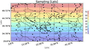
Figure 3: Sampling various models for training along latitude lines, as the temperature gradient is more apparent in this direction.

After sampling these models, one can simply train these few models. Predictions can be made simply by evaluating these trained models at all locations and selecting the trained model with the smallest latitude distance between selected and trained locations (then, longitude distance is given second priority) or some weighted distance of [lats, lons], with latitude having a high weight.

3.1 Clustering based

Although the approach outlined above makes logical sense, it highly depends on the problem at hand. The nature of the underlying problem is frequently unknown to us, so we may not always be able to determine which geospatial direction is the most important. When it comes to more general problems, we prefer clustering, where the idea is to cluster geospatial locations based on some metric distance. In this case, the basic assumption is that the nearby locations have similar climate behaviour.

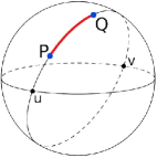
Figure 4: Shortest distance between $P\&Q$

In the context of clustering spatiotemporal data, some authors have suggested that DBSCAN performs well in some cases [35], but this was not the case for our dataset. As we know, the shortest distance between two points on the Earth’s surface is not the shortest in the Euclidean sense due to the curvature of the Earth’s surface. Thus, the optimal solution is to use a different distance, such as geodesic or haversine, as a distance metric for the nearest-neighbour algorithm. Haversine distance can be mathematically written as

$r=$ radius of earth, $r\approx 6367\mathrm{~{}km}$
$\varphi_{1},\varphi_{2}$ are the latitude of point $P$ and the latitude of point $Q$ as shown in Figure 4, $\lambda_{1},\lambda_{2}$ are the longitude of point $P$ and the longitude of point $Q$, respectively.

There are many options to use such distance metrics for nearest-neighbor lookup, one can simply use Balltree from sklearn, or scipy’s cKDTree based, here we can give distance argument as (’haversine’), other option is to use K-Means with haversine distance.

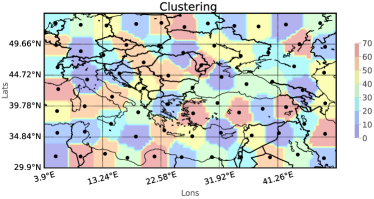
Figure 5: The models for training are sampled using Haversine distance based clustering.

Finally, after clustering, the idea is to train the location-specific models on centered time series (the mean of all time series within a particular cluster), as indicated by the black dots in Figure 5, and then perform prediction by evaluating the trained models on each location within its respective cluster.

3.2 Snapshot LSTM

In order to use the vector autoregression or LSTM model, we vectorize a temperature field at each time instant, also called the ”method of snapshots in the fluid community” Consider a multivariate or multiple time series $\mathbf{Y}\in\mathbb{R}^{K\times T},$ where $K$ is the number of variables (here in our case, K is the dimension of the vectorized temperature field or the number of longitude-latitude grid points), and $T$ is the total number of time-stamps. This reshaped dataset now consists of a single spatial dimension instead of two and a temporal dimension, i.e., each row of $\mathbf{Y}$ represents a time series at a specific geospatial location, while each column corresponds to the temperature at all locations at a specific time instant (vectorized temperature field). The main problem with this method is that it removes inter-spatial relationships, which are often crucial, but here this approach allowed us to use classical LSTM to evolve these snapshots in time as a multivariate time series.

3.3 Matrix autoregression

In the above discussion of the snapshot approach, we have seen the main problem of vectorizing the maps (2D-temperature field), i.e., it removes the inter-spatial correlations. To tackle this problem, we use the matrix auto-regression, originally proposed in [36]; the main idea of matrix autoregression (MAR) is to generalize the vector autoregression (VAR).

Consider a spatiotempoal tensor $\underline{\mathbf{X}}\in\mathbb{R}^{M\times N\times T}$ at each time $t$, we have a weather map as matrix $\mathbf{X}_{t}$ of size $M\times N$, where $M,N$ correspond to spatial locations/dimensions. The authors have formulated the first order MAR model in a bilinear structure as shown below.

$$\mathbf{X}_{t}=\mathbf{A}\mathbf{X}_{t-1}\mathbf{B^{\top}}+\mathcal{E}_{t},$$ (3)

where $\mathcal{E}_{t}$ is the error matrix at time $t$, $\mathbf{A}$ having size of $M\times M$, and $\mathbf{B}$ having size of $N\times N$. The authors claim that framing matrix values time series as above has two main benefits:

• This formulation offers substantial reduction of parameters as compared vectorization based. That is, MAR only needs $(M^{2}+N^{2})$, while VAR for the same data will require $(MN)^{2}$ parameters.

• The coefficients $\mathbf{A}$ &  $\mathbf{B}$ are well interpretable depending upon problem at hand.

The authors propose many approaches to find the coefficient matrices; here, we will use the alternating least-squares-based method. Finally, we can formulate the optimization problem as below:

$$\quad\min_{\mathbf{A},\mathbf{B}}\frac{1}{2}\sum_{t=2}^{1}\left\|\mathbf{X}_{t}-\mathbf{A}\mathbf{X}_{t-1}\mathbf{B}^{\top}\right\|_{F}^{2}$$

The above problem has a proven closed-form solution, which can be found by simply setting the corresponding partial derivative of the objective function to zero, and update rules can be written as:

$$\mathbf{A}^{k+1} =\left(\sum_{t=2}^{T}\mathbf{X}_{t}\mathbf{B}^{k}\mathbf{X}_{t-1}^{\top}\right)\left(\sum_{t=2}^{T}\mathbf{X}_{t-1}\left(\mathbf{B}^{k}\right)^{\top}\mathbf{B}^{k}\boldsymbol{X}_{t-1}^{\top}\right)^{-1}$$

$$\mathbf{B}^{k+1} =\left(\sum_{t=2}^{T}\mathbf{X}_{t}^{\top}\mathbf{A}^{k+1}\mathbf{X}_{t-1}\right)\left(\sum_{t=2}^{T}\mathbf{X}_{t-1}^{\top}\left(\mathbf{A}^{k+1}\right)^{\top}\mathbf{A}^{k+1}\mathbf{X}_{t-1}\right)^{-1}$$

Once the optimal coefficients have been determined, the prediction can simply be found as:

$$\mathbf{\hat{X}}_{t+1}=\mathbf{A}_{opt}\mathbf{X}_{t}\mathbf{B}_{opt}^{\top},$$

3.4 ConvLSTM

Researchers proposed a model in [29] that enabled LSTM to include spatial features by using convolution operations within LSTM, i.e., convolution operator in input-to-state and state-to-state transition. Cell outputs, hidden states, input gate, output gate, and forget gate are 3D tensors with the last two dimensions corresponding to the spatial dimension, and they use spatial features inherited in design automatically, as shown in Figure 6.

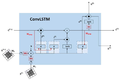
Figure 6: ConvLSTM cell

The key equations of ConvLSTM cell is shown below:

$$\mathbf{i}_{t} =\sigma\left(\mathbf{W}_{ix}*\mathbf{X}_{t}+\mathbf{W}_{ih}*\mathbf{H}_{t-1}+\mathbf{W}_{ic}\circ\mathbf{C}_{t-1}+\mathbf{b}_{i}\right)$$ (4)

$$\mathbf{f}_{t} =\sigma\left(\mathbf{W}_{fx}*\mathbf{X}_{t}+\mathbf{W}_{fh}*\mathbf{H}_{t-1}+\mathbf{W}_{fc}\circ\mathbf{C}_{t-1}+\mathbf{b}_{f}\right)$$

$$\mathbf{S}_{t} =\tanh\left(\mathbf{W}_{cx}*\mathbf{X}_{t}+\mathbf{W}_{ch}*\mathbf{H}_{t-1}+\mathbf{b}_{c}\right)$$

$$\mathbf{C}_{t} =\mathbf{f}_{t}\circ\mathbf{C}_{t-1}+\mathbf{i}_{t}\circ\mathbf{S}_{t}$$

$$\mathbf{o}_{t} =\sigma\left(\mathbf{W}_{ox}*\mathbf{X}_{t}+\mathbf{W}_{oh}*\mathbf{H}_{t-1}+\mathbf{W}_{oc}\circ\mathbf{C}_{t}+\mathbf{b}_{o}\right)$$

$$\mathbf{H}_{t} =\mathbf{o}_{t}\circ\tanh\left(\mathbf{C}_{t}\right),$$

where $\circ$ denotes Hadamard product and * denotes convolution operation.

Encoder-decoder prediction network:
The future prediction model can be formed by stacking multiple ConvLSTM layers [29]. We use an encoder-decoder network, in which the encoder part compresses the whole input sequence into a hidden tensor, and the forecaster (decoder) part decodes the compressed part to generate predictions. The similar classical LSTM model was very successful in generating predictions as proposed in [37], [38]. The encoder-forecaster model shown in Figure 7 also copies the last hidden state and cell outputs from the encoder to the decoder/forecasting part, and similarly for other ConvLSTM decoder layers. This architecture has been quite successful in precipitation nowcasting [29].

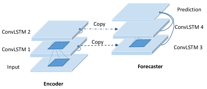
Figure 7: Encoder-Forecaster Network

3.5 Tensor based dynamic mode decomposition

DMD is a dimensionality reduction algorithm that decomposes spatiotemporal data into different spatial/DMD modes, each with a temporal behaviour defined by a single frequency and growth/decay rate (DMD eigenvalues) [39], [40]. This is similar to matrix factorization, in which a spatiotemporal matrix is decomposed into spatial and temporal factors. DMD has a wide range of applications; most notably, it is capable of multivariate time series forecasting.

Consider a time-series data vectors $\left\{\mathbf{z}_{0},\ldots,\mathbf{z}_{m}\right\}$, where each snapshots $\mathbf{z}_{k}\in\mathbb{R}^{n}.$ Assuming some linear dynamical system generated the data, we can write

$$\mathbf{z}_{k+1}=\mathbf{A}\mathbf{z}_{k}$$ (5)

where matrix $\mathbf{A}$ is unknown, $\mathbf{z}_{k}=\mathbf{z}(k\Delta t)$; $\Delta t$ being fixed sampling rate. The main aim of DMD is to approximate $\mathbf{A}$, such that $\mathbf{Y}\approx\mathbf{AX},$ where $\mathbf{X}$ and $\mathbf{Y}$ are snapshot matrices arranged as, $\mathbf{X\triangleq\left[\begin{array}[]{lll}z_{0}&\cdots&z_{m-1}\end{array}\right],\quad Y\triangleq\left[\begin{array}[]{lll}z_{1}&\cdots&z_{m}\end{array}\right],}$ we can find bit-fit operator $\mathbf{A}=\mathbf{YX^{\dagger}}$ [41], but this operation is computationally expensive. Instead, we use DMD to approximate the dynamics of $\mathbf{A}$ by finding its eigenmodes and eigenvalues, as shown below:

After finding the DMD modes and eigenvalues, one can easily reconstruct or forecast the snapshots a shown below:

$$\mathbf{z}_{k}=\boldsymbol{\Phi}\boldsymbol{\Lambda}^{k}\boldsymbol{\Phi}^{\dagger}\mathbf{z}_{0},$$ (6)

where $\boldsymbol{\Phi}$ is the matrix of whose columns are DMD modes ($\hat{\varphi}^{\prime}$s), and $\boldsymbol{\Lambda}$ is a diagonal matrix containing of eigenvectors of $\tilde{\mathbf{A}},$ since $\mathbf{A}$ and $\tilde{\mathbf{A}}$ share same eigenvalue spectrum.

This approach is reasonable, but it only applies to the 2D case, i.e., we have a snapshot vector at each time point. But what if each snapshot itself is a matrix or we have a 3D data tensor? Using tensor train decomposition [42], researchers in [43] have extended the DMD to higher order tensors.
TT-format
Let $\underline{\mathbf{A}}\in\mathbb{R}^{n_{1}\times\cdots\times n_{d}}$ be the $d$th order tensor with $n_{l}$ denoting the size of the $l$th mode. In TT-format $\underline{\mathbf{A}}$ is factored into $d$ core tensors $\underline{\mathbf{A}}^{(l)}\in$ $\mathbb{R}^{{r}_{l-1}\times n_{1}\times r_{l}}$, where $r_{0}=r_{d}=1,\text{ where }r_{l}$ is TT-rank of $l$th mode. Simply, any element of $\underline{\mathbf{A}}$ is given by

$$\underline{\mathbf{A}}_{i_{1},\ldots,i_{d}}=\sum_{k_{0}=1}^{r_{0}}\ldots\sum_{k_{d}=1}^{r_{d}}\underline{\mathbf{A}}_{k_{0},i_{1},k_{1}}^{(1)}\cdots\cdot\underline{\mathbf{A}}_{k_{d-1},i_{d},k_{d}}^{(d)},$$ (7)

where indices are written in subscripts. Furthermore, for two vectors $\boldsymbol{v}\in\mathbb{R}^{n_{1}}$ and $w\in\mathbb{R}^{n_{2}}$, the tensor product $\boldsymbol{v}\otimes\boldsymbol{w}\in\mathbb{R}^{n_{1}\times n_{2}}$ is given by $(\boldsymbol{v}\otimes\boldsymbol{w})_{i,j}=\left(\boldsymbol{v}\cdot\boldsymbol{w}^{\top}\right)_{i,j}=$ $v_{i}\cdot w_{j}.$ Using this we can write

$$\underline{\mathbf{A}}=\sum_{k_{0}=1}^{r_{0}}\ldots\sum_{k_{d}=1}^{r_{d}}\underline{\mathbf{A}}_{k_{0},:,k_{1}}^{(1)}\otimes\cdots\otimes\underline{\mathbf{A}}_{k_{d-1},:,k_{d}}^{(d)},$$ (8)

Matlab-like notation. Matricizations and vectorizations can be described as, let $\underline{\mathbf{A}}_{i_{1},\ldots,i_{l},:,i_{l+1}\ldots,i_{d}}$, where $1\leq$ $l\leq d-1.$ For the two ordered subsets $N^{\prime}=\left\{n_{1},\ldots,n_{l}\right\}$ and $N^{\prime\prime}=$ $\left\{n_{l+1},\ldots,n_{d}\right\}$ of $N=\left\{n_{1},\ldots,n_{d}\right\}$, the matricization of $\underline{\mathbf{A}}$ with respect to $N^{\prime}$ and $N^{\prime\prime}$ is denoted by $\underline{\mathbf{A}}\mid\begin{array}[]{l}N^{\prime\prime}\\ N^{\prime}\end{array}\in\mathbb{R}^{\left(n_{1}\cdots\cdot n_{l}\right)\times\left(n_{l+1}\cdots\cdot n_{d}\right)}$, i.e; concatenating the mode-$l$ fibers of $\underline{\mathbf{A}}$ [43]. The special case where $N^{\prime}=N$ and $N^{\prime\prime}=\varnothing$, is simply vectorization of $\underline{\mathbf{A}}$ is denoted by vec$(\underline{\mathbf{A}})\in\mathbb{R}^{n_{1}\cdots\cdot\cdot n_{d}}$
Tensor-train DMD
So, we have seen the central part of the DMD algorithm is to find the pseudo-inverse first; let us see how we compute pseudo-inverse in TT-format. The procedure for computing pseudo-inverse has been already proposed in [43] and [44]. For, tensor based DMD, consider $m$ snapshots of $d$-dimensional tensor-trains $\underline{\mathbf{X}},\underline{\mathbf{Y}}\in\mathbb{R}^{n_{1}\times\cdots\times n_{d}\times m}$, where $\underline{\mathbf{X}}_{:,\ldots,:,i+1}\in\mathbb{R}^{n_{1}\times\cdots\times n_{d}}$ for $i=0,\ldots,m-1$ and $\underline{\mathbf{Y}}_{:,\ldots,:,i}$ for $i=1,\ldots,m.$ Let $r_{0},\ldots,r_{d+1}$ and $s_{0},\ldots,s_{d+1}$ be the TT-ranks of $\underline{\mathbf{X}}$ and $\underline{\mathbf{Y}}$, respectively. Now, let $\mathbf{X},\mathbf{Y}\in\mathbb{R}^{n_{1}\cdots.\cdot n_{d}\times m}$ be the matricizations of $\underline{\mathbf{X}}$ and $\underline{\mathbf{Y}}$ around $m$, where we contract the dimensions $n_{1},\ldots,n_{d}$ such that every column of $\mathbf{X}$ and $\mathbf{Y}$ is the vectorization of the corresponding $m=n_{d+1}$ snapshot, respectively. To efficiently compute tensor-train DMD (TT-DMD) only with matrix products, first, we do TT-decomposition of $\underline{\mathbf{X}}$ and matricize to $\mathbf{X}$, $\ni$ $\mathbf{X}=\mathbf{M}\boldsymbol{\Sigma}\mathbf{N}$ with

$$\mathbf{M}=\left(\sum_{k_{0}=1}^{r_{0}}\cdots\sum_{k_{d-1}=1}^{r_{d-1}}\underline{\mathbf{X}}_{k_{0},:,k_{1}}^{(1)}\otimes\cdots\otimes\underline{\mathbf{X}}_{k_{d-1},:,:}^{(d)}\right)\Biggm{|}\begin{array}[]{l}r_{d}\\ n_{1},\ldots,n_{d}\end{array}$$

$\mathbf{N}=\left.\left(\underline{\mathbf{X}}_{:,:,k_{d+1}}^{(d+1)}\right)\right|_{r_{d}}^{m}$, with $\boldsymbol{\Sigma}$ being the diagonal matrix with singular values on its diagonal elements, which are computed by performing the SVD of $\underline{\mathbf{X}}^{(d)}\mid\begin{array}[]{l}r_{d}\\ r_{d-1},n_{d}\end{array}$ Also, $\mathbf{N}$ is equivalent to the last core $\underline{\mathbf{X}}^{(d+1)}$, which is a matrix because $r_{d+1}=k_{d+1}=1$. The is similar to SVD for matrices, but SVD and this matricization after TT-decomposition are different. $\mathbf{M}\in\mathbb{R}^{n_{1}\cdots n_{d}\times r_{d}}$ is computed by $d$ cores (first) of $\underline{\mathbf{X}}$ is left-orthogonal, using procedure for tensor-train-factorization highlighted algorithm in [42], and this represents some share of tensor structure of $\underline{\mathbf{A}}$ when folding back to full-format. Here also, we assume a linear relationship between the pairs of data vectors, i.e.

$$\mathbf{Y=AX}$$ (9)

with $\mathbf{A}\in\mathbb{R}^{n_{1}\cdots n_{d}\times n_{1}\cdots n_{d}},$ where $\mathbf{A=Y\cdot X^{\dagger}}$. Finally, pseudoinverse $\mathbf{X^{\dagger}}$ can be as:

$$\mathbf{X^{\dagger}}=\left(\underline{\mathbf{X}}\Biggm{|}\begin{array}[]{l}m\\ n_{1},\ldots,n_{d}\end{array}\right)^{\dagger}=\mathbf{N}^{\top}\boldsymbol{\Sigma}^{-1}\mathbf{M}^{\top}$$

Similarly, the unfolding $\underline{\mathbf{Y}}$ can be written as a matrix product as:

$$\begin{split}&\mathbf{Y}=\left.\underline{\mathbf{Y}}\right|_{n_{1},\ldots,n_{d}}^{m}\\ &=\left.\left(\sum_{l_{0}=1}^{s_{0}}\cdots\sum_{l_{d-1}=1}^{s_{d-1}}\underline{\mathbf{Y}}_{l_{0},:,l_{1}}^{(1)}\otimes\ldots\otimes\underline{\mathbf{Y}}_{l_{d-1},:,:}^{(d)}\right)\right|_{n_{1},\cdots,n_{d}}^{s_{d}}\left.\cdot\underline{\mathbf{Y}}^{(d+1)}\right|_{s_{d}}^{m}=\mathbf{PQ}\end{split}$$

Here we don’t have to care about specific properties of the tensor cores of $\mathbf{Y}$. Finally on combining the representations of $\mathbf{X}^{\dagger}$ and $\mathbf{Y}$, we generalize the procedure to tensor-form. So, the reduced matrices can be written as

$$\tilde{\mathbf{A}}=\mathbf{M}^{\top}\cdot\mathbf{PQ\cdot N}^{\top}\boldsymbol{\Sigma}^{-1}$$ (10)

For effcient compuataion, we split the above expression into different parts. First, consider $\mathbf{M^{\top}\cdot P}$, any element can be found by

$$\begin{split}&\left(\mathbf{M}^{\top}\cdot\mathbf{P}\right)_{i,j}=\\ &\sum_{k_{0}=1}^{r_{0}}\cdots\sum_{k_{d-1}=1}^{r_{d-1}}\sum_{l_{0}=1}^{s_{0}}\cdots\sum_{l_{d-1}=1}^{s_{d-1}}\left(\underline{\mathbf{X}}_{k_{0},:,k_{1}}^{(1)}\right)^{\top}\underline{\mathbf{Y}}_{l_{0},:,l_{1}}^{(1)}\ldots\left(\underline{\mathbf{X}}_{k_{d-1},:,i}^{(d)}\right)^{\top}\underline{\mathbf{Y}}_{l_{d-1},:,j}^{(d)}\end{split}$$

This is following this expression:

$$\operatorname{vec}(\underline{\mathbf{X}})^{\top}\cdot\operatorname{vec}(\underline{\mathbf{Y}})=\Pi_{l=1}^{d}\left(\underline{\mathbf{X}}^{(l)}\right)^{\top}\cdot\underline{\mathbf{X}}^{(l)}.$$

Here again, we will use TT-format for computation of $\mathbf{M}^{\top}\cdot\mathbf{P}$ since we only need to reshape some TT-cores. For efficient computation, we use Algorithm 4 from [42]. Assuming tensor train-ranks of $\underline{\mathbf{X}}$ and $\underline{\mathbf{Y}}$ are small with respect to the whole state-space. The tensor ranks $r_{d}$ and $s_{d}$ are both bounded by $m$. Finally, we can write $\mathbf{Q}\cdot\mathbf{N}^{\dagger}=\left.\underline{\mathbf{Y}}^{(d+1)}\right|_{s_{d}}^{m}\cdot\left(\underline{\mathbf{X}}^{(d+1)}\Biggm{|}\begin{array}[]{l}m\\ r_{d}\end{array}\right)^{\dagger}$
Considering the exact DMD algorithm proposed in Algorithm-2 in [45], we can simple compute DMD modes of $\tilde{\mathbf{A}}$. If $\lambda_{1},\ldots,\lambda_{p}$ are the eigenvalues of $\tilde{\mathbf{A}}$ corresponding to the eigenvectors $\boldsymbol{w}_{1},\ldots,\boldsymbol{w}_{p}\in\mathbb{R}^{r_{d+1}}$, then the vectorized DMD modes $\mathbf{\varphi}_{1},\ldots,\mathbf{\varphi}_{p}\in\mathbb{R}^{n_{1}\cdots\cdot\cdot n_{d}}$ of $\mathbf{A},$

$$\mathbf{\varphi}_{j}=\left(1/\lambda_{j}\right)\cdot\mathbf{P}\mathbf{Q}\cdot\mathbf{N}^{\dagger}\boldsymbol{\Sigma}^{-1}\cdot\mathbf{w}_{j},$$ (11)

for $j=1,\ldots,p$. To sum-up all these modes in single tensor i.e, $\underline{\boldsymbol{\Phi}}\in\mathbb{R}^{n_{1}\times\cdots\times n_{d}\times p}$ which is given by:

$$\underline{\boldsymbol{\Phi}}=\sum_{l_{0}=1}^{s_{0}}..\sum_{l_{d}=1}^{s_{d}}\underline{\mathbf{Y}}_{l_{0},:,l_{1}}^{(1)}\otimes.. \otimes\underline{\mathbf{Y}}_{l_{d-1},:,l_{d}}^{(d)}$$ (12)

$$\otimes\left(\mathbf{Q}\cdot\mathbf{N}^{\dagger}\boldsymbol{\Sigma}^{-1}\cdot\mathbf{W}\cdot\boldsymbol{\Lambda}^{-1}\right)_{l_{d},:^{\prime}}$$

again with $\operatorname{vec}\left(\underline{\boldsymbol{\Phi}}_{:,\ldots,:,j}\right)=\mathbf{\varphi}_{j}$ and $\boldsymbol{\Lambda}$ is a diagonal matrix of eigenvectors. So, the summary of the whole algorithm is shown below: see [43].
Finally, we can sum up the algorithm as below in Algorithm 2

We use the tensor-train framework to generalize the DMD forecasting algorithm, which is basically designed to predict vectors, as studied in [46], to higher-order tensors (2D matrices here). The algorithm below is designed to work with the original weather map dimensions and is able to reconstruct and predict matrices directly. The Algorithm 3 is shown below:

where $\Omega$ is vector of logarithm of eigenvalues. Also, the sample code is available

4 Experiments and discussion of the results

4.1 Dataset description

The NASA Power database was used. This is a global database of regular weather data, primarily for agricultural purposes. The spatial resolution is 0.5°x0.5°, with a temporal resolution of one day. We collected the maximum temperature time series (TMAX in degrees Celsius). The collected dataset is formatted as a time series at various latitude-longitude coordinates between the 30-Oct-2015 and 15-November-2020 time range, containing approximately 1844 timestamps at each coordinate point (i.e., the length of each time series). We chose specific geographic locations, such as a range of lat $\times$ lon: [30.0° to 54.5°] $\times$ [4.0° to 51.5°]. Around 4700 latitude-longitude points ($50\times 94$) are contained within this latitude-longitude range. This latitude-longitude range encompasses parts of Europe and Central Asia.

4.2 Evaluation criteria

In order to measure the model’s performance, we can use different kinds of metrics. These metrics estimate the model’s forecasting precision. Generally, these metrics measure the error between actual data and predicted data. Depending upon the need, we may use scale-dependent metrics, i.e., on the same scale on which the data itself is, for example, root mean square error (RMSE), mean absolute error (MAE), or scale-independent, which are more general, for example, absolute percentage error (MAPE, SMAPE). Here, we have used the following metrics to measure the performance, see [47].

1. Root mean square error:

   $$\mathbf{RMSE}=\sqrt{\frac{1}{n}\sum_{i=1}^{n}\left(y_{i}^{\mathrm{obs}}-y_{i}^{\mathrm{pred}}\right)^{2}}$$

2. Mean absolute error:

   $$\mathbf{MAE}=\frac{\sum_{i=1}^{n}\left|y_{i}^{\mathrm{obs}}-y_{i}^{\mathrm{pred}}\right|}{n}$$

3. Symmetric mean absolute percentage error:

   $$\mathbf{SMAPE}=\frac{100\%}{n}\sum_{t=1}^{n}\frac{\left|y^{\mathrm{pred}}_{i}-y^{\mathrm{obs}}_{i}\right|}{\left(\left|y^{\mathrm{obs}}_{i}\right|+\left|y^{\mathrm{pred}}_{i}\right|\right)/2}$$

   where $y_{i}^{\mathrm{obs}}$ and $y_{i}^{\mathrm{pred}}$ are the real and predicted data observations, respectively.

4.3 Numerical Experiments

The experiments are performed to predict the temperature time series across all longitude-latitude coordinate points ([30.0° to 54.5°] $\times$ [4.0° to 51.5°]), in the following way: First, we make the short-term predictions (i.e., the next seven days) using all the spatiotemporal forecasting approaches described in section 3, and then, based on a performance comparison, we select models which are computationally less expensive to make long-term predictions (250 steps ahead) and compare their performance to ensure their ability to predict temperature fields for multiple time steps ahead.

Train-test split: In the short-term prediction case, we choose a subset of data from 2015-10-30 to 2019-12-07 for training and 2019-12-08 to 2019-12-14 for testing. For the long-term prediction experiments, the training data is the same as that of the short-term case, but the test data ranges from 2019-12-08 to 2020-08-13.

4.3.1 Short-term predictions:

Training procedure:  For sampling and clustering-based approaches, we sampled 70 locations as described in the section 3, similarly as shown in Figure 3, Figure 5 respectively. We trained a 2-layer LSTM model at each of the 70 selected locations. We trained each LSTM model on centred time series (time series calculated by averaging all time series within a given cluster/sub-region), with a time-lag (a.k.a., lookback) = 5 days, output sequence length = 7, with 500 epochs, and a learning rate = 2.3e-4. We optimize these models over MSE loss, i.e.,

$$L(y,\hat{y})=\frac{1}{N}\sum_{i=0}^{N}(y-{\hat{y}}_{i})^{2}$$

where $y,~{}\hat{y}$, are the actual and predicted values, respectively. The training procedure of Snapshot LSTM is identical to the above methods, except that in this model, the input data is the set of vectorized temperature fields (a set of vectors where in each vector, we have temperature values collected across all locations).

ConvLSTM data preparation is similar to the LSTM data preparation, except that frames are used instead of vectors; data instances consist of twelve frames; five for input and seven for prediction. Similarly to what was proposed in the original work [29], the four-layer ConvLSTM model shown in Figure 7 was trained with each layer containing a hidden size of 32 and a $3\times 3$ kernel size. This model was also optimized on MSE loss with Adam optimizer $(lr=5e-3$, decay rate$=0.9)$ for 50 epochs. ConvLSTM, TT-DMD, and matrix autoregression (MAR) models work with the original dimensions of data and are capable of directly predicting a two-dimensional $(50\times 94)$ temperature field for next seven time steps, i.e, $\underline{\mathbf{X}}_{predition}\in\mathbb{R}^{50\times 94\times steps}$. The matrix auto-regression (MAR) of order one was chosen as the baseline, and the MAR coefficient was learned using the ALS algorithm with $500$ iterations. We prepared shifted tensors $(\underline{\mathbf{X}},\underline{\mathbf{Y}}),$ for TT-DMD and used Algorithm 2 as in section 3.5 to find TT-DMD modes ($\underline{\boldsymbol{\Phi}}$) and eigenvalues with $rank(R)=70$ (optimal by grid search).

Results:

We compared the 7-steps-ahead predictions of the various spatiotemporal models. In Figure 8, we plotted the target temperature field and corresponding prediction across all the locations on 2020-08-13 (this is the prediction’s seventh time-step). We can see that the ConvLSTM and TT-DMD models predict the temperature field quite well. However, the MAR predictions on the seventh-time step is the least accurate since this MAR is only of order one. Also, it is interesting to note that models based on dimensionality reduction are pretty good at predicting regional temperature, despite being trained on a small number of selected locations.

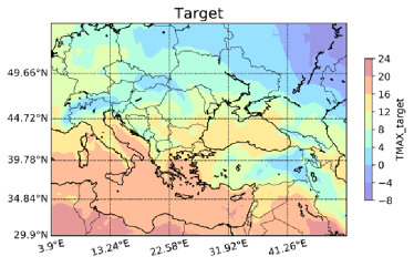
Figure 8: Target temperature distribution 2020-08-13

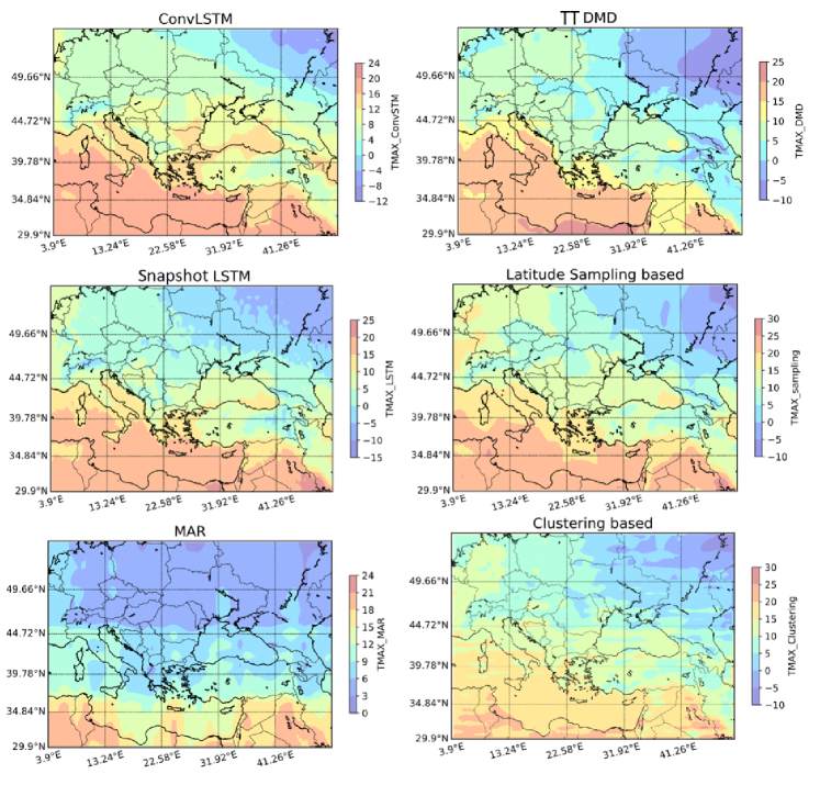
Figure 8: Predicted temperature distributions using different forecasting methods 2020-08-13

The RMSE distribution across the locations is shown in Figure 9, and we infer that the RMSE for a ConvLSTM is least, while others have nearly similar. The plots show that error in the sampling-based model is uniformly distributed, whereas error in other models is much higher in some regions.

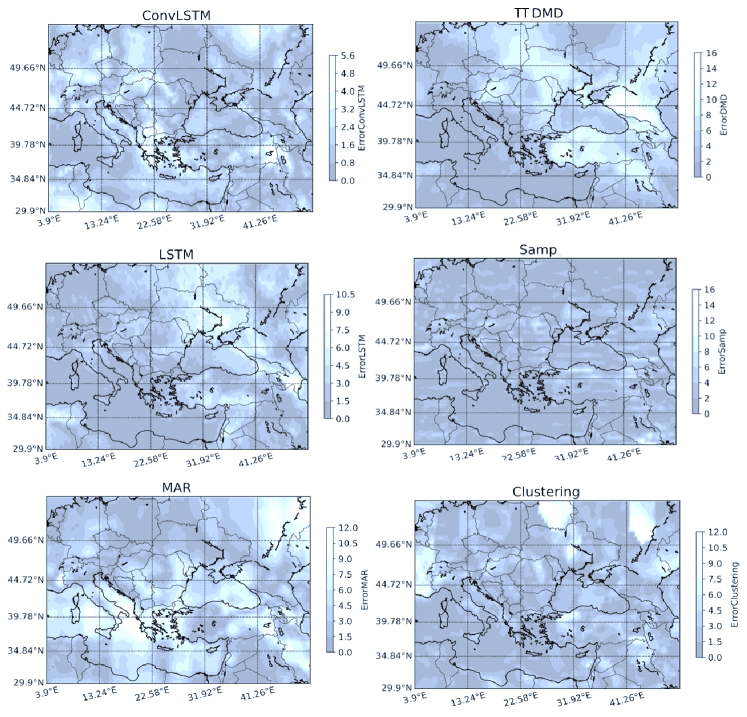
Figure 9: Regional RMSE distribution between predictions and target

To draw a general conclusion about these models, we compared their performance for seven-step predictions, recorded their training and inference times and other error metrics, and presented the results in Table 1.

Table 1: Overall Comparison of different spatiotemporal models on short-term prediction (7 step ahead)

Metrics	ConvLSTM	TT-DMD	MAR	LSTM (Snapshot)	Sampling Lats based	Clustering based
RMSE	1.70	3.01	4.45	2.88	2.46	2.95
MAE	1.37	2.98	3.68	2.34	1.97	2.79
SMAPE	22.89	45.70	52.23	49.72	30.09	33.80
Time (training+inference)	4mins + 54 sec	91 sec	84 sec	4 min, 44 sec + 1 mins, 19 sec	14 mins, 2 sec + 7 mins, 37 sec	14 mins, 49 sec + 8 mins, 3 sec

Based on the results presented in Table 1, we can infer that ConvSTM performed the best while MAR performed the worst in terms of the error metric. The rest show roughly similar behaviour. TT-DMD is optimal in terms of the total time taken for data fitting and predictions. Models based on clustering and sampling took significantly longer to train and evaluate, suggesting they are not best suited for long-term predictions. In conclusion, we can say that spatiotemporal models that work directly with the original dimensions work significantly better since they capture both spatial and temporal correlations. Furthermore, TT-DMD is an excellent choice when quick spatiotemporal predictions are required.

4.3.2 Long-term predictions:

We concluded in the preceding section that ConvLSTM, TT-DMD, and MAR models could be easily tested for long-term predictions because they are computationally less expensive. This section validates their success for long-term forecasting (250-time steps ahead).

Training procedure:  The ConvLSTM training procedure is the same as the short-term prediction training procedure discussed in the previous section, except that the data instances now have a longer lookback (i.e., to incorporate more past states/history) and forecast horizons; we used thirty frames, fifteen for input and fifteen for prediction and used iterative (recursive) prediction strategy to get 250 step predictions, as shown in [48], [49]. The training for TT-DMD and MAR is the same, but the prediction length has been increased to 250 steps. Although rolling forecasting mechanisms can be used in MAR or TT-DMD, we limited our technique in this work to simple prediction mechanisms only.

Results:

We compare the predictions of MAR, ConvLSTM, and TT-DMD with the target, as shown in Figure 10. From the plots, we can deduce that the MAR model is incapable of correctly predicting multiple steps ahead, whereas TT-DMD and ConvLSTM predictions are quite close to target frames. According to the predictions, TT-DMD is superior to ConvLSTM at capturing spatial information for the first few steps, and as shown in Figure 12, TT-DMD also has the lowest frame-wise normalized root mean square error (NRMSE) for the first eight steps, then it starts increasing and becomes slightly higher than ConvLSTM, but is far better than MAR throughout the prediction length.

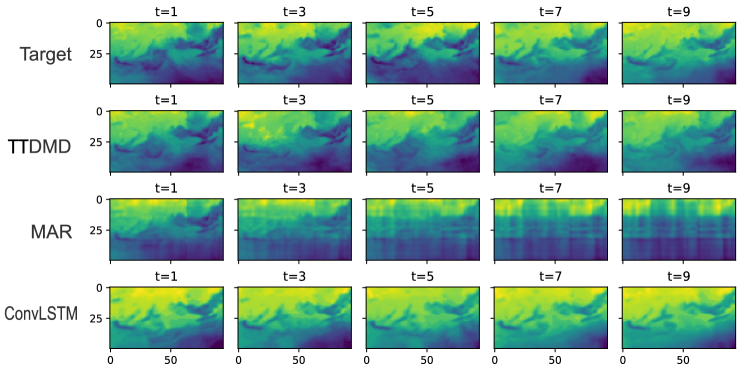
Figure 10: Performance comparison of frame-wise predictions over multiple future time steps.

We chose four arbitrary locations to compare the performance of models at different latitude-longitude coordinate points, i.e., we took four time fibres (individual temperature time series) of the spatiotemporal prediction tensor, $\underline{\mathbf{X}}_{predition}$  and observed how they evolved over time. These time series are depicted in Figure 11.

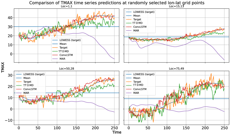
Figure 11: Performance comparison of at randomly selected locations over latitude-longitude grids

We compared the predictions to the target, the target’s mean, and the local weighted scatterplot smoothness (LOWESS), as shown in the plots, and found that ConvLSTM and TT-DMD are successful in capturing trends, and their trajectories are close to the target, whereas MAR predictions are unable to follow the target trajectory. The reason for this is that MAR does not incorporate long-range space-time correlations because it is only of order-1 matrix-auto-regressor, i.e., MAR(1). This implies that our model must take into account long-range correlations in both space and time, like TT-DMD and ConvLSTM. Finally, the MAR, ConvLSTM, and TT-DMD predictions are compared to the target time-series at multiple locations (30 distinct locations), and the mean RMSE and SMAPE metrics are listed in Table. 2.

Table 2: Here, we compared individual location-wise MAR, TT-DMD, and ConvLSTM time fibers predictions over 30 different locations and presented average errors.

Metrics	TT-DMD	MAR	ConvLSTM
RMSE	4.677	12.248	3.298
SMAPE	19.093	59.188	14.511

The spatiotemporal prediction ability among these models is assessed in this case by comparing each model’s 100 prediction steps frame by frame (slice-wise) with the target. For each time step, we calculated frame-wise mean-square error (MSE), normalised root mean-square error (NMSE), structural similarity index (SSIM), and peak signal-to-noise ratio (PSNR). As shown in Figure 12, frame-wise errors increased significantly for MAR but remained nearly constant for TT-DMD and ConvLSTM. ConvLSTM error is smaller and smoother than TT-DMD error, implying that ConvLSTM is more stable and better than TT-DMD. Furthermore, we can see that ConvLSTM has a higher structural similarity index than TT-DMD and MAR, while NRMSE is lowest for TT-DMD.

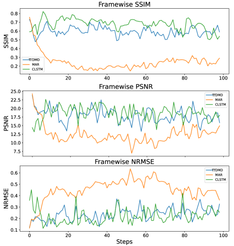
Figure 12: We plotted framewise SSIM, PSRN, and NRMSE to compare performance and see how prediction errors evolve over time (prediction time steps).

In Table 3, we listed the mean performance (mean errors/accuracy across all 250 prediction slices) of models on given metrics and discovered that ConvLSTM predictions are 68% structurally similar to the target, while TT-DMD predictions are 66% similar. ConvLSTM has the greatest average PSNR, followed by TT-DMD. TT-DMD has the lowest mean NRMSE, followed by ConvLSTM. The performance of MAR is the worst among them.

Table 3: Framewise-comparison between MAR, TT-DMD, and ConvLSTM

Metric	TT-DMD	MAR	ConvLSTM
MSE	1143.08	4327.14	986.86
NRMSE	0.22	0.46	0.23
PSNR	19.13	13.74	20.83
SSIM	0.66	0.24	0.68

To get a broader picture of these models, we summarised the primary findings in Table 4, where we emphasised the key advantages and shortcomings of various forecasting models.

Table 4: Summary Table

Model	Pros	Cons
ConvLSTM	1. The prediction accuracy is good. 2. It is quite effective in capturing spatiotemporal correlations. 3. To boost performance, we can easily incorporate an attention mechanism. 4. Suitable for long-term forecasting.	1. A significant amount of training data and time are needed for this model. 2. In comparison to classical LSTM, it performs poorly when data across successive time intervals does not vary significantly.
TT-DMD	1. This is a better choice when dataset is small. 2. Captures spatiotemporal correlations. 3. Provides faster and more accurate forecasts for shorter forecasting horizons. 4. Training and inference time is short.	1. It struggles to learn from massive datasets. 2. It does not work well with the irregularly sampled dataset (i.e., time series data must be regularly sampled).
MAR	1. This model generalizes vector autoregression. 2. It captures inter-spatial correlations. 3. Reduces computational cost. 4. It works well when the forecast horizon is very small.	1. Prediction error is very high. 2. Cannot capture long-term correlations easily. 3. Optimizing model coefficients becomes a challenge on increasing MAR order.
Snapshot LSTM	1. Ease of implementation and data preparation. 2. Works good for most of the prediction problems	1. Prohibits long lookbacks for high dimensional vectors. 2. Removes inter-spatial correlation by vectoriza- tion (in spatiotemporal datasets). 3. Does not perform well for data with high spatial correlations.
Sampling and Clustering based	1. In terms of computational cost and the inclusion of spatiotemporal correlations, these models are better than training separate models for each coordinate point. 2. These models are intuitive and easy to implement. 3. Easy to include domain knowledge. For example, we used temperature gradient knowledge to sample the models for training from latitude- longitude space.	1. Assumes nearby locations have similar weather- patterns, which doesn’t always hold. It may not hold at certain locations, such as shores, river- banks, and islands. 2. These models are not suitable for long-term predictions since their training and inference time is relatively high.

5 Concluding remarks

We present various purely data-driven approaches for spatiotemporal forecasting, and we show how to condition these models for forecasting weather states over multiple locations simultaneously by exploiting spatiotemporal correlations. We observed that incorporating spatiotemporal correlations improves performance and reduces the computational cost, as can be seen by comparing LSTM to the ConvLSTM model, in which simple multiplications are replaced with convolutions inside the classical LSTM layer to incorporate spatiotemporal correlations effectively. We proposed a TT-DMD spatiotemporal forecasting model and found that its predictions are comparable to those of the ConvLSTM without the need for training, and it significantly reduces computational time. We evaluated the proposed methods for both short-term and long-term forecasting to ensure their capability to predict temperature fields for multiple time steps ahead. Moreover, the proposed model is an excellent choice for quick and short-term spatiotemporal predictions. It should, however, be noted that TT-DMD is struggling to learn spatiotemporal correlations with massive, incomplete, or irregularly sampled datasets. Future work should therefore take care of these two issues.

References

-
[1]
IRENA, Innovation landscape brief: Advanced forecasting of
variable renewable power generation, international renewable energy agency,
isbn 978-92-9260-179-9, IRENA, Abu Dhabi, 2020.
URL www.irena.org - [2] L. F. Richardson, Weather prediction by numerical process, Cambridge (University Press), 1922. 4°. Pp. xii + 236. 30s.net, Vol. 48, 1922, pp. 282–284. doi:https://doi.org/10.1002/qj.49704820311.
- [3] J. Charney, The use of the primitive equations of motion in numerical prediction, Tellus 7 (1) (1955) 22–26. doi:https://doi.org/10.1111/j.2153-3490.1955.tb01138.x.
- [4] J. G. Charney, R. FjÖrtoft, J. V. Neumann, Numerical integration of the barotropic vorticity equation, Tellus 2 (4) (1950) 237–254. doi:10.3402/tellusa.v2i4.8607.
- [5] E. Kalnay, Atmospheric Modeling, Data Assimilation and Predictability, Cambridge University Press, 2002. doi:10.1017/CBO9780511802270.
- [6] G. Evensen, Sequential data assimilation with a nonlinear quasi‐geostrophic model using monte carlo methods to forecast error statistics, Journal of Geophysical Research 99 (1994) 10143–10162.
- [7] M. Tolstykh, A. Frolov, Some current problems in numerical weather prediction, Izvestiya Atmospheric and Oceanic Physics 41 (2005) 285–295.
- [8] G. E. P. Box, G. Jenkins, Time Series Analysis, Forecasting and Control, Holden-Day, Inc., USA, 1990.
- [9] J. Delleur, M. Kavvas, Stochastic models for monthly rainfall forecasting and synthetic generation, Journal of Applied Meteorology 17 (1978) 1528–1536. doi:10.1175/1520-0450(1978)017<1528:SMFMRF>2.0.CO;2.
- [10] Q. Zhang, B.-D. Wang, B. He, Y. Peng, M.-L. Ren, Singular Spectrum Analysis and ARIMA Hybrid Model for Annual Runoff Forecasting, Water Resources Management: An International Journal, Published for the European Water Resources Association (EWRA) 25 (11) (2011) 2683–2703. doi:10.1007/s11269-011-9833-y.
- [11] P. Chen, A. Niu, D. Liu, W. Jiang, B. Ma, Time series forecasting of temperatures using sarima: An example from nanjing, IOP Conference Series: Materials Science and Engineering 394 (2018) 052024. doi:10.1088/1757-899X/394/5/052024.
- [12] K. Hornik, M. Stinchcombe, H. White, Multilayer feedforward networks are universal approximators, Neural Networks 2 (5) (1989) 359–366. doi:https://doi.org/10.1016/0893-6080(89)90020-8.
- [13] T. Nishijima, Universal approximation theorem for neural networks (2021). arXiv:2102.10993.
- [14] X. Yu, Comparison of support vector machine and extreme gradient boosting for predicting daily global solar radiation using temperature and precipitation in humid subtropical climates: A case study in china, Energy Conversion and Management 164 (03 2018). doi:10.1016/j.enconman.2018.02.087.
- [15] V. Vapnik, The nature of statistical learning theory, Springer science & business media, 1999. doi:https://doi.org/10.1007/978-1-4757-3264-1.
- [16] T. Chen, T. He, M. Benesty, V. Khotilovich, Y. Tang, H. Cho, K. Chen, et al., Xgboost: extreme gradient boosting, R package version 0.4-2 1 (4) (2015) 1–4.
- [17] C. Rensheng, K. Ersi, J. Yang, S. Lyu, W. Zhao, Validation of five global radiation models with measured daily data in china, Energy Conversion and Management 45 (2004) 1759–1769. doi:10.1016/j.enconman.2003.09.019.
- [18] B. Scott, Estimation of solar radiation in australia from rainfall and temperature observations, Agricultural and Forest Meteorology 106 (2001) 41–59. doi:10.1016/S0168-1923(00)00173-8.
- [19] M. Qi, G. P. Zhang, Trend time–series modeling and forecasting with neural networks, IEEE Transactions on Neural Networks 19 (5) (2008) 808–816. doi:10.1109/TNN.2007.912308.
- [20] E. Mutlu, I. Chaubey, H. Hexmoor, S. G. Bajwa, Comparison of artificial neural network models for hydrologic predictions at multiple gauging stations in an agricultural watershed, Hydrological Processes 22 (26) (2008) 5097–5106. doi:https://doi.org/10.1002/hyp.7136.
- [21] S. Wei, H. Yang, J. Song, K. Abbaspour, Z. Xu, A wavelet-neural network hybrid modelling approach for estimating and predicting river monthly flows, Hydrological Sciences Journal 58 (2) (2013) 374–389. doi:10.1080/02626667.2012.754102.
-
[22]
M. Das, S. K. Ghosh,
Data-driven approaches for
spatio-temporal analysis: A survey of the state-of-the-arts, J. Comput. Sci.
Technol. 35 (3) (2020) 665–696.
doi:10.1007/s11390-020-9349-0.
URL https://doi.org/10.1007/s11390-020-9349-0 - [23] X. Shi, D.-Y. Yeung, Machine learning for spatiotemporal sequence forecasting: A survey, ArXiv abs/1808.06865 (2018).
-
[24]
L. Anselin, Spatial
Econometrics: Methods and Models, Studies in Operational Regional Science,
Springer Netherlands, 2013.
URL https://books.google.ru/books?id=G47tCAAAQBAJ - [25] R. Pace, R. Barry, J. Clapp, M. Rodriquez, Spatio-temporal autoregressive models of neighborhood effects, The Journal of Real Estate Finance and Economics 17 (1998) 15–33. doi:10.1023/A:1007799028599.
- [26] Y. Lecun, L. Bottou, Y. Bengio, P. Haffner, Gradient-based learning applied to document recognition, Proceedings of the IEEE 86 (11) (1998) 2278–2324. doi:10.1109/5.726791.
- [27] R. A. Rajagukguk, R. A. A. Ramadhan, H.-J. Lee, A review on deep learning models for forecasting time series data of solar irradiance and photovoltaic power, Energies 13 (24) (2020). doi:10.3390/en13246623.
- [28] D. Qin, J. Yu, G. Zou, R. Yong, Q. Zhao, B. Zhang, A novel combined prediction scheme based on cnn and lstm for urban pm2.5 concentration, IEEE Access 7 (2019) 20050–20059. doi:10.1109/ACCESS.2019.2897028.
- [29] X. Shi, Z. Chen, H. Wang, D.-Y. Yeung, W.-k. Wong, W.-c. Woo, Convolutional lstm network: A machine learning approach for precipitation nowcasting, in: Proceedings of the 28th International Conference on Neural Information Processing Systems - Volume 1, NIPS’15, MIT Press, Cambridge, MA, USA, 2015, p. 802–810.
- [30] W. chun Woo, Application of optical flow techniques to rainfall nowcasting, 2014.
- [31] R. C. Nascimento, Y. M. Souto, E. S. Ogasawara, F. A. M. Porto, E. Bezerra, Stconvs2s: Spatiotemporal convolutional sequence to sequence network for weather forecasting, ArXiv abs/1912.00134 (2021).
- [32] S. Bai, J. Z. Kolter, V. Koltun, An empirical evaluation of generic convolutional and recurrent networks for sequence modeling, ArXiv abs/1803.01271 (2018).
- [33] D. Tran, H. Wang, L. Torresani, J. Ray, Y. LeCun, M. Paluri, A closer look at spatiotemporal convolutions for action recognition, 2018 IEEE/CVF Conference on Computer Vision and Pattern Recognition (2018) 6450–6459.
- [34] C. G. Wang K, Sun J, Effect of altitude and latitude on surface air temperature across the qinghai-tibet plateau, j. mt. sci, 2011. doi:doi.org/10.1007/s11629-011-1090-2.
- [35] N.-A. Le-Khac, M. Bue, M. Whelan, M.-T. Kechadi, A clustering-based data reduction for very large spatio-temporal datasets, in: L. Cao, J. Zhong, Y. Feng (Eds.), Advanced Data Mining and Applications, Springer Berlin Heidelberg, Berlin, Heidelberg, 2010, pp. 43–54.
- [36] R. Chen, H. Xiao, D. Yang, Autoregressive models for matrix-valued time series, Journal of Econometrics 222 (1, Part B) (2021) 539–560, annals Issue:Financial Econometrics in the Age of the Digital Economy. doi:https://doi.org/10.1016/j.jeconom.2020.07.015.
- [37] I. Sutskever, O. Vinyals, Q. V. Le, Sequence to sequence learning with neural networks, in: Z. Ghahramani, M. Welling, C. Cortes, N. D. Lawrence, K. Q. Weinberger (Eds.), Advances in Neural Information Processing Systems 27: Annual Conference on Neural Information Processing Systems 2014, December 8-13 2014, Montreal, Quebec, Canada, 2014, pp. 3104–3112.
- [38] N. Srivastava, E. Mansimov, R. Salakhutdinov, Unsupervised learning of video representations using lstms, in: Proceedings of the 32nd International Conference on International Conference on Machine Learning - Volume 37, ICML’15, JMLR.org, 2015, p. 843–852.
- [39] P. J. SCHMID, Dynamic mode decomposition of numerical and experimental data, Journal of Fluid Mechanics 656 (2010) 5–28. doi:10.1017/S0022112010001217.
- [40] J. N. Kutz, Data-Driven Modeling and Scientific Computation: Methods for Complex Systems and Big Data, Oxford University Press, Inc., USA, 2013.
- [41] R. Penrose, On best approximate solutions of linear matrix equations, Mathematical Proceedings of the Cambridge Philosophical Society 52 (1) (1956) 17–19. doi:10.1017/S0305004100030929.
- [42] I. V. Oseledets, Tensor-train decomposition, SIAM Journal on Scientific Computing 33 (5) (2011) 2295–2317. doi:10.1137/090752286.
- [43] S. Klus, P. Gelß, S. Peitz, C. Schütte, Tensor-based dynamic mode decomposition, Nonlinearity 31 (7) (2018) 3359–3380. doi:10.1088/1361-6544/aabc8f.
- [44] K. Fujii, Y. Kawahara, Dynamic mode decomposition in vector-valued reproducing kernel hilbert spaces for extracting dynamical structure among observables, Neural Networks 117 (2019) 94–103. doi:10.1016/j.neunet.2019.04.020.
- [45] J. H. Tu, , C. W. Rowley, D. M. Luchtenburg, S. L. Brunton, J. N. K. and, On dynamic mode decomposition: Theory and applications, Journal of Computational Dynamics 1 (2) (2014) 391–421. doi:10.3934/jcd.2014.1.391.
- [46] E. V. Filho, P. Lopes dos Santos, A dynamic mode decomposition approach with hankel blocks to forecast multi-channel temporal series, IEEE Control Systems Letters 3 (3) (2019) 739–744. doi:10.1109/LCSYS.2019.2917811.
- [47] A. Botchkarev, Performance metrics (error measures) in machine learning regression, forecasting and prognostics: Properties and typology, ArXiv abs/1809.03006 (2018).
- [48] N. H. An, D. T. Anh, Comparison of strategies for multi-step-ahead prediction of time series using neural network, in: 2015 International Conference on Advanced Computing and Applications (ACOMP), 2015, pp. 142–149. doi:10.1109/ACOMP.2015.24.
- [49] R. Chandra, S. Goyal, R. Gupta, Evaluation of deep learning models for multi-step ahead time series prediction, IEEE Access 9 (2021) 83105–83123. doi:10.1109/ACCESS.2021.3085085.