Millionfold improvement in multivibration-feedback optomechanical refrigeration via auxiliary mechanical coupling

Abstract

The simultaneous ground-state refrigeration of multiple vibrational modes is a prerequisite of observing significant quantum effects of multiple-vibration systems. Here we propose how to realize a giant amplification in the net-refrigeration rates based on cavity optomechanics, and to largely improve the cooling performance of multivibration modes beyond the resolved-sideband regime. By employing an auxiliary mechanical coupling (AMC) between two mechanical vibrations, the dark mode, which is induced by the coupling of these vibrational modes to a common optical mode and cuts off cooling channels, can be fully removed. We use fully analytical treatments for the effective mechanical susceptibilities and net-cooling rates, and find that when the AMC is turned on, the amplification of the net-refrigeration rates can be observed by more than six orders of magnitude. In particular, we reveal that the simultaneous ground-state cooling beyond the resolved-sideband regime arises from the introduced AMC, without which it vanishes. Our work paves a route for the quantum control of multiple vibrational modes in the bad-cavity regime.

I Introduction

Cavity optomechanics Bowen2015CRCpress ; Kippenberg2008Science ; Meystre2013AP ; Aspelmeyer2014RMP provides a promising platform to explore mechanical properties of quantum system via optical means and to manipulate cavity-field statistics by mechanically changing the boundary of a cavity Rabl2011PRL ; Nunnenkamp2011 ; Liao2012PRA ; Liao2013PRA ; Liao2013 ; Wang2013PRL ; Liu2013PRL0 ; Vitali2007PRL ; Agarwal2010PRA ; Genes2011PRA ; Cirio2017PRL ; Xu12015PRA ; Hou2015PRA ; Zou2020OE ; Bai2016PRA ; Yang2017OE ; Lai2020PRAOMIT ; Xu2021PRA ; Qian2021PRA ; Wu2018PRApplied ; Qin2018PRL ; Zippilli2018PRA ; Wang2015 ; Li2019 ; Jiao2020 . As a prominent application closely related to this optomechanical platform, optomechanical refrigeration has become a hot research topic Wilson-Rae2007PRL ; Marquardt2007PRL ; Genes2008PRA ; Chan2011Nature ; Teufel2011Nature ; Clarkl2017Nature . This is due to the fact that for observing significantly quantum effects of systems, a prerequisite is to cool these systems to their quantum ground states by effectively suppressing their thermal noise. Until now, cooling a single mechanical mode to its quantum ground state of optomechanical systems, has been mainly achieved by the resolved-sideband-refrigeration Wilson-Rae2007PRL ; Marquardt2007PRL ; Genes2008PRA ; Chan2011Nature ; Teufel2011Nature ; Clarkl2017Nature and feedback-aided-refrigeration Mancini1998PRL ; Steixner2005PRA ; Bushev2006PRL ; Rossi2017PRL ; Rossi2018Nature ; Conangla2019PRL ; Tebbenjohanns2019PRL ; Sommer2019PRL ; Guo2019PRL ; Sommer2020PRR mechanisms, which are preferable in the good-cavity and bad-cavity regimes, respectively.

In recent years, much attention has been paid to multivibration-mode systems Bowen2015CRCpress ; Kippenberg2008Science ; Meystre2013AP ; Aspelmeyer2014RMP . This is because these systems can provide an incomparable platform to investigate topological energy transfer Xu2016Nature , macroscopic mechanical coherence Mancini2002PRL ; Tian2004PRL ; Massel2012Nc ; Mari2013PRL ; Matheny2014PRL ; Zhang2015PRL ; Ockeloen-Korppi2018 ; Riedinger2018Nature ; Stefano2019PRL ; Qin2019npj ; Kotler2021Science ; Ockeloen-Korppi2021Science , and quantum many-body effects Heinrich2011PRL ; Xuereb2012PRL ; Ludwig2013PRL ; Xuereb2014PRL ; Xuereb2015NJP ; Mahmoodian2018PRL ; Rabl2010NP . In particular, they have been widely applied in high-performance sensors Massel2011Nature ; Huang2013PRL ; Bernier2016PRL , quantum mechanical computers Masmanidis2007science ; Yamaguchi2008NN , and nonreciprocal devices Malz2018PRL ; Shen2016NP ; Shen2018NC ; Shen2022arXiv ; Fang2017NP ; Xu2019Nature ; Mathew2018arXiv ; Yang2020NC ; SanavioPRB2020 . These applications relevant to multivibration-mode systems, however, are fundamentally limited by thermal noise. To effectively suppress these thermal noise, simultaneously cooling these multivibration systems to their quantum ground states, becomes an important and urgent task. Although cooling a single vibrational mode to its quantum ground state has been realized in both optical Chan2011Nature ; Teufel2011Nature ; Clarkl2017Nature ; MXu2020PRL ; Qiu2020PRL ; Liu2013PRL ; Liu2014PRA ; Wang2011PRL ; Li2011PRB ; Yan2016PRA ; Liao2011PRA ; Machnes2012PRL ; Lai2020PRARC ; Lai2018PRA ; Lai2021PRA1 ; Lai2021PRA2 and microwave Grajcar2008PRB ; Zhang2009PRA ; Liberato2011PRA ; Xue2007PRB ; You2008PRL ; Nori2008NP ; Xiang2013RMP domains, the simultaneous cooling of multiple vibrational modes remains an outstanding challenge in cavity optomechanics. The physical origin behind this challenge can be explained by cooling suppression due to dark modes Scully1997QO ; Agarwal2013QO , which are induced by the coupling of multiple vibrational modes to a common cavity-field mode Shkarin2014PRL ; Sommer2019PRL ; Massel2012Nc ; Genes2008NJP ; Ockeloen-Korppi2019PRA ; Kuzyk2017PRA ; Huang2021arXiv ; Liu2021arXiv ; Lai2022PRL ; Lai2022PRR1 ; Lai2022PRR2 .

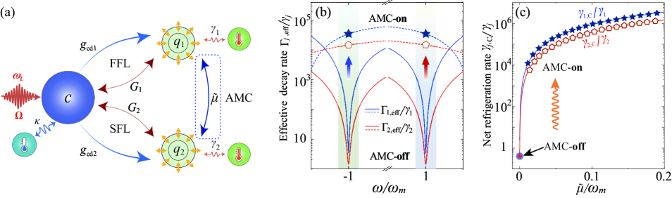
Figure 1: (a) Schematic diagram of a three-mode optomechanical system. An optical mode $c$ (with frequency $\omega_{c}$ and decay rate $\kappa$) is coupled to two vibrational modes $q_{j}$ (with frequency $\omega_{j}$ and damping rate $\gamma_{j}$) via radiation-pressure couplings (with strength $G_{j}$), and the two vibrational modes are coupled to each other through an AMC (with strength $\tilde{u}$). The cavity-field mode interacts with the vacuum bath, and the two vibrational modes are connected to their high-temperature heat baths. Note that the FFL denotes the strength of the first feedback loop, and the SFL describes the strength of the second feedback loop. (b) The effective mechanical damping $\Gamma_{j,\mathrm{eff}}(\omega)$ of the $j$th vibrational mode versus the frequency $\omega$, when the system operates without ($\tilde{\mu}=0$, solid curves) and with ($\tilde{\mu}/\omega_{m}=0.02$, dashed curves) the AMC. (c) The net-refrigeration rate $\gamma_{j,\mathrm{C}}(\omega)$ of the $j$th vibrational mode as a function of the AMC strength $\tilde{\mu}$. The parameters used are: $\omega_{j=1,2}=\omega_{m}=2\pi\times 10^{7}$, $G_{1}/\omega_{m}=0.4$, $G_{2}=0.7G_{1}$, $g_{\mathrm{cd1}}=1$, $g_{\mathrm{cd2}}=0.6$, $\kappa/\omega_{m}=4$, $\gamma_{j}/\omega_{m}=10^{-6}$, $\vartheta=0.8$, $\omega_{\mathrm{fb}}/\omega_{m}=3$, and $\bar{n}_{1}=\bar{n}_{2}=10^{3}$.

In this paper, based on the feedback-cooling mechanism, we proposed a dark-mode-removing method to achieve the simultaneous ground-state cooling of the two mechanical modes in the unresolved-sideband regime. This is realized by employing auxiliary mechanical coupling (AMC) to break the symmetry of the system, and, then, both dark and bright modes can be effectively controlled. By obtaining the exact analytical results of the net-cooling rates, effective mechanical susceptibilities, and steady-state mean phonon numbers, we find that when the AMC is turned on in the system, a giant amplification in the net-refrigeration rates can be observed. Specifically, these net-refrigeration rates can be amplified to more than six orders of magnitude by properly tuning the AMC strength.

In particular, we show that the tremendously amplified net-refrigeration rates can result in a giant improvement for the refrigeration performance of the mechanical modes. Without AMC, the two vibrational modes cannot be efficiently cooled due to an inefficient net-cooling rate. However, when the AMC is turned on, the simultaneous ground-state cooling of these vibrations is achieved beyond the resolved-sideband regime, owing to the giant amplification in the net-cooling rates. Remarkably, we reveal that the larger is the feedback-loop strength of the resonator, the better is the cooling efficiency of this resonator. Physically, the introduced AMC offers an effective strategy to remove the dark mode and, in turn, to rebuild cooling channels for extracting thermal phonons stored in the dark mode. This study could pave the way for studying quantum control and observing quantum mechanical coherence effects involving multiple vibrational modes.

II Model and hamiltonian

As shown in Fig. 1(a), we consider a three-mode optomechanical system, in which two vibrational modes are optomechanically coupled to a common optical mode. An AMC between the two vibrational modes is introduced to improve the net-cooling rates and the cooling performance of the system. To control the system, an external control laser with amplitude $\Omega$ and frequency $\omega_{L}$ is applied to the optical cavity. The Hamiltonian of the system reads ($\hbar=1$)

$$H_{0}= \;\omega_{c}c^{{\dagger}}c+\sum_{j=1}^{2}(\frac{1}{2m_{j}}p_{x,j}^{2}+\frac{1}{2}m_{j}\tilde{\omega}_{j}^{2}x_{j}^{2})-\lambda_{1}c^{\dagger}cx_{1}-\lambda_{2}c^{\dagger}cx_{2}$$

$$+\mu(x_{1}-x_{2})^{2}+\Omega(c^{\dagger}e^{-i\omega_{L}t}+ce^{i\omega_{L}t}),$$ (1)

where $c$ ($c^{{\dagger}}$) denotes the annihilation (creation) operator of the optical mode. The operators $p_{x,j}$ ($j=1,2$) and $x_{j}$ are, respectively, the momentum and position operators of the $j$th vibrational mode, with frequency $\tilde{\omega}_{j}$ and mass $m_{j}$. The $\lambda_{j}$ terms describe the optomechanical interactions between the optical mode and the $j$th vibrational mode, and the $\mu$ term denotes the AMC between the two vibrations. Note that the FFL denotes the strength of the first feedback loop, and the SFL describes the strength of the second feedback loop.

For the convenience of studying the system, we introduce the dimensionless position ($q_{j}=\sqrt{m_{j}\omega_{j}}x_{j}$) and momentum ($p_{j}=\sqrt{1/(m_{j}\omega_{j})}p_{x,j}$) operators, and the normalized resonance frequencies $\omega_{j}=\sqrt{\tilde{\omega}_{j}^{2}+2\mu/{m_{j}}}$ for $j=1,2$. In a rotating frame, defined by $\rm exp$$(-i\omega_{L}c^{{\dagger}}ct)$, the system Hamiltonian (1) becomes

$$H= \;\Delta_{c}c^{\dagger}c+\sum_{j=1}^{2}\dfrac{\omega_{j}}{2}(q_{j}^{2}+p_{j}^{2})-\tilde{\lambda}_{1}c^{\dagger}cq_{1}-\tilde{\lambda}_{2}c^{\dagger}cq_{2}$$

$$-2\tilde{\mu}q_{1}q_{2}+\Omega(c^{\dagger}+c),$$ (2)

where $\tilde{\lambda}_{1}=\lambda_{1}\sqrt{1/(m_{1}\omega_{1})}$, $\tilde{\lambda}_{2}=\lambda_{2}\sqrt{1/(m_{2}\omega_{2})}$, $\tilde{\mu}=\mu\sqrt{1/(m_{1}m_{2}\omega_{1}\omega_{2})}$, and $\Delta_{c}=\omega_{c}-\omega_{L}$. We here need to emphasize that the Hamiltonian in Eq. (2) is the starting point of our analysis and numerical simulations.

III Langevin equations and steady-state mean phonon numbers

In this section, we obtain the Langevin equations of the system, analyze a cold-damping feedback-cooling scheme, and derive the steady-state average phonon numbers.

III.1 Langevin equations

We consider the case where the two vibrational modes are subjected to quantum Brownian forces, and the optical mode interacts with their vacuum baths. Then, the quantum Langevin equations can be used to describe the evolution of the system:

$$\dot{c} =-[\kappa+i(\Delta_{c}-\tilde{\lambda}_{1}q_{1}-\tilde{\lambda}_{2}q_{2})]c-i\Omega+\sqrt{2\kappa}c_{in},$$

$$\dot{q}_{j} =\omega_{j}p_{j},~{}~{}j=1,2$$

$$\dot{p}_{1} =-\omega_{1}q_{1}+2\tilde{\mu}q_{2}+\tilde{\lambda}_{1}c^{\dagger}c-\gamma_{1}p_{1}+\xi_{1},$$

$$\dot{p}_{2} =-\omega_{2}q_{2}+2\tilde{\mu}q_{1}+\tilde{\lambda}_{2}c^{\dagger}c-\gamma_{2}p_{2}+\xi_{2},$$ (3)

where the operators $c_{in}$ and $\xi_{j}$ are, respectively, the input noise operator of the cavity-field mode and the Brownian noise operator resulting from the coupling of the corresponding vibrational modes to the thermal baths. These noise operators satisfy zero mean values and the following correlation functions:

$$\langle c_{in}(t)c_{in}^{\dagger}(t^{{}^{\prime}})\rangle=\delta(t-t^{{}^{\prime}}),$$

$$\langle c_{in}^{\dagger}(t)c_{in}(t^{{}^{\prime}})\rangle=\langle c_{in}^{\dagger}(t^{{}^{\prime}})c_{in}(t)\rangle=0,$$

$$\langle\xi_{j}(t)\xi_{j}(t^{{}^{\prime}})\rangle=\frac{1}{2\pi}\dfrac{\gamma_{j}}{\omega_{j}}\int\omega e^{-i\omega(t-t^{{}^{\prime}})}\left[1+\coth(\dfrac{\hbar\omega}{2k_{\mathrm{B}}T_{j}})\right]d\omega,$$ (4)

where $k_{\mathrm{B}}$ is the Boltzmann constant, and $T_{j}$ is the thermal bath temperature associated with the $j$th vibrational mode.

We assume that the cavity is strongly driven, and this allows us to linearize the dynamics of the system by writing each operator as the sum of their averages and fluctuations, i.e., $A=\langle A\rangle_{ss}+\delta A$ for $A\in\{c,c^{{\dagger}},q_{j},p_{j}\}$. By neglecting higher-order fluctuation terms, the linearized quantum Langevin equations, which are described by the quadrature fluctuations $\delta X=(\delta c^{{\dagger}}+\delta c)/\sqrt{2}$ and $\delta Y=i(\delta c^{\dagger}-\delta c)/\sqrt{2}$, are given by

$$\delta\dot{X}= -\kappa\delta X+\Delta\delta Y+\sqrt{2\kappa}X_{in},$$

$$\delta\dot{Y}= -\kappa\delta Y-\Delta\delta X+G_{1}\delta q_{1}+G_{2}\delta q_{2}+\sqrt{2\kappa}Y_{in},$$

$$\delta\dot{q}_{j}= \;\omega_{j}\delta p_{j},~{}~{}j=1,2,$$

$$\delta\dot{p}_{1}= -\omega_{1}\delta q_{1}+2\tilde{\mu}\delta q_{2}+G_{1}\delta X-\gamma_{1}\delta p_{1}+\xi_{1},$$

$$\delta\dot{p}_{2}= -\omega_{2}\delta q_{2}+2\tilde{\mu}\delta q_{1}+G_{2}\delta X-\gamma_{2}\delta p_{2}+\xi_{2},$$ (5)

where $X_{in}=(\delta c_{in}^{{\dagger}}+\delta c_{in})/\sqrt{2}$ and $Y_{in}=i(\delta c_{in}^{\dagger}-\delta c_{in})/\sqrt{2}$ are the corresponding Hermitian input noise quadratures, and the parameter $\Delta=\Delta_{c}-\tilde{\lambda}\langle q_{1}\rangle_{ss}-\tilde{\lambda}\langle q_{2}\rangle_{ss}$ is the normalized effective driving detuning. Moreover, $G_{1}=\sqrt{2}\tilde{\lambda}_{1}\langle c\rangle_{ss}$ and $G_{2}=\sqrt{2}\tilde{\lambda}_{2}\langle c\rangle_{ss}$ are the effective optomechanical coupling strengths, with $\langle c\rangle_{ss}=-i\Omega/(\kappa+i\Delta)$. Note that the phase reference of the cavity field $\langle c\rangle_{ss}$ is assumed to be real and positive.

III.2 Cold-damping feedback

To realize the cold-damping feedback refrigeration, the case of $\Delta=0$ is considered, so that the highest sensitivity for the position measurements of the vibrational modes can be achieved Mancini1998PRL ; Steixner2005PRA ; Bushev2006PRL ; Rossi2017PRL ; Rossi2018Nature ; Conangla2019PRL ; Tebbenjohanns2019PRL ; Sommer2019PRL ; Guo2019PRL ; Sommer2020PRR . This feedback-refrigeration mechanism is essentially different from the sideband-cooling mechanism requiring the red-sideband resonance, i.e., $\Delta=\omega_{j}$ Wilson-Rae2007PRL ; Marquardt2007PRL ; Genes2008PRA ; Chan2011Nature ; Teufel2011Nature ; Clarkl2017Nature . By using a negative-derivative feedback, the effective decay rate of the mechanical mode can be largely developed by the cold-damping feedback technique.

Physically, the position of the two mechanical modes is measured through the phase-sensitive detection of the cavity output field, and, then, the readout of the cavity output field is fed back onto the two vibrational modes by applying feedback forces. The intensity of these feedback forces is proportional to the time derivative of the output signal, and, therefore, to the velocity of the mechanical modes. Then, the linearized quantum Langevin equations in Eq. (5) become

$$\delta\dot{X}=-\kappa\delta X+\sqrt{2\kappa}X_{\mathrm{in}},$$

$$\delta\dot{Y}=-\kappa\delta Y+G_{1}\delta q_{1}+G_{2}\delta q_{2}+\sqrt{2\kappa}Y_{\mathrm{in}},$$

$$\delta\dot{q}_{j}=\omega_{j}\delta p_{j},$$

$$\delta\dot{p}_{1}= -\omega_{1}\delta q_{1}+2\tilde{\mu}\delta q_{2}+G_{1}\delta X-\gamma_{1}\delta p_{1}+\xi_{1}$$

$$-\int^{t}_{-\infty}g_{1}(t-s)\delta Y^{\mathrm{est}}(s)ds,$$

$$\delta\dot{p}_{2}= -\omega_{2}\delta q_{2}+2\tilde{\mu}\delta q_{1}+G_{2}\delta X-\gamma_{2}\delta p_{2}+\xi_{2}$$

$$-\int^{t}_{-\infty}g_{2}(t-s)\delta Y^{\mathrm{est}}(s)ds,$$ (6)

where the convolution term $\int^{t}_{-\infty}g_{j}(t-s)\delta Y^{\mathrm{est}}(s)ds$ $(j=1,2)$ denotes the feedback force acting on the $j$th vibrational mode. These feedback forces depend on the past dynamics of the detected quadrature $\delta Y$, which is driven by a weighted sum of the fluctuations of the vibrational modes. Here, the causal kernel is defined by

$$g_{j}(t)=g_{\mathrm{cd},j}\dfrac{d}{dt}[\theta(t)\omega_{\mathrm{fb}}e^{-\omega_{\mathrm{fb}}t}],$$ (7)

where $g_{\mathrm{cd},j}$ and $\omega_{\mathrm{fb}}$ are the dimensionless feedback gain and feedback bandwidth associated the $j$th vibrational mode, respectively. In Eq. (7), we have assumed that the electronic loop can provide an instantaneous feedback onto the system, and this assumption is included in the argument of the Heaviside function $\theta(t)$ Genes2008PRA ; Sommer2019PRL ; Sommer2020PRR . This assumes fast electronics that can respond much quicker than the oscillation time of the system Genes2008PRA ; Sommer2019PRL ; Sommer2020PRR . The estimated intracavity phase quadrature $\delta Y^{\mathrm{est}}$ results from the homodyne measurement of the output quadrature $\delta Y^{\mathrm{out}}(t)$. Here we generalize the usual input-output relation,

$$\delta Y^{\text{out}}(t)=\sqrt{2\kappa}\delta Y(t)-Y^{\text{in}}(t),$$ (8)

to the case of a nonunit detection efficiency by modeling a detector with quantum efficiency $\vartheta$ with an ideal detector preceded by a beam splitter (with transmissivity $\sqrt{\vartheta}$), which mixes the incident field with the uncorrelated vacuum field $Y^{\upsilon}(t)$. Then, we obtain the generalized input-output relation,

$$Y^{\text{out}}(t)=\sqrt{\vartheta}[\sqrt{2\kappa}\delta Y(t)-Y^{\mathrm{in}}(t)]-\sqrt{1-\vartheta}Y^{\upsilon}(t).$$ (9)

The estimated phase quadratures $\delta Y^{\text{est}}(t)$ are obtained as

$$\delta Y^{\text{est}}(t)=\frac{Y^{\text{out}}(t)}{\sqrt{2\vartheta\kappa}}=\delta Y(t)-\frac{Y^{\text{in}}(t)+\sqrt{\vartheta^{-1}-1}Y^{\upsilon}(t)}{\sqrt{2\kappa}}.$$ (10)

Below, we seek the steady-state solution of Eq. (6) by solving it in the frequency domain with the Fourier transform. $r(t)=(1/2\pi)^{1/2}\int_{-\infty}^{\infty}e^{-i\omega t}\tilde{r}(\omega)d\omega$ (for $r=\delta X$, $\delta Y$, $\delta q_{j}$, $\delta p_{j}$, $\xi_{j}$, $X_{\text{in}}$, and $Y_{\text{in}}$), and consequently the quantum Langevin equations in Eq. (6), with the cold-damping feedback, can be solved in the frequency domain. Based on the steady-state solution, we can calculate the spectra of the position and momentum operators for two mechanical modes, and, then, the steady-state mean phonon numbers in these resonators can be obtained by integrating the corresponding fluctuation spectra.

III.3 Final average phonon numbers

The final steady-state average phonon numbers in the $j$th vibrational mode can be obtained by

$$n^{f}_{j}=\dfrac{1}{2}[\langle\delta q^{2}_{j}\rangle+\langle\delta p^{2}_{j}\rangle-1],~{}~{}~{}j=1,2,$$ (11)

where $\langle\delta q^{2}_{j}\rangle$ and $\langle\delta p^{2}_{j}\rangle$ are the variances of the position and momentum operators, respectively. We solve Eq. (6) in the frequency domain and integrate the corresponding fluctuation spectra, and then, the corresponding variances can be obtained as

$$\langle\delta q^{2}_{j}\rangle=\dfrac{1}{2\pi}\int^{\infty}_{-\infty}S_{q_{j}}(\omega)d\omega,$$

$$\langle\delta p^{2}_{j}\rangle=\dfrac{1}{2\pi\omega^{2}_{j}}\int^{\infty}_{-\infty}\omega^{2}S_{q_{j}}(\omega)d\omega.$$ (12)

The fluctuation spectra of the position and momentum operators are defined by

$$S_{A}(\omega)=\int^{\infty}_{-\infty}e^{-i\omega\tau}\langle\delta A(t+\tau)\delta A(t)\rangle_{\mathrm{ss}}d\tau,~{}(A=q_{j},p_{j})$$ (13)

where $\langle\cdot\rangle_{\mathrm{ss}}$ denotes the steady-state average of the system. The fluctuation spectra in the frequency domain are expressed as

$$\langle\delta\tilde{A}(\omega)\delta\tilde{A}(\omega^{\textquotesingle})\rangle_{\mathrm{ss}}=S_{A}(\omega)\delta(\omega+\omega^{{}^{\prime}}).$$ (14)

Thus, in the frequency domain, we can solve this system and obtain the analytical results of the steady-state average phonon numbers.

III.4 Dark-mode effect and its removing

We next show the dark-mode effect and its removing from the two-vibrational-mode optomechanical system. For convenience, we introduce the annihilation (creation) operators of the two vibrational modes: $b_{j}=(q_{j}+ip_{j})/\sqrt{2}$ [$b_{j}^{\dagger}=(q_{j}-ip_{j})/\sqrt{2}$]. In the process of optomechanical cooling, the beam-splitting-type interactions (corresponding to the rotating-wave interaction term) between these bosonic modes dominate the linearized couplings in this system. By considering a red-detuned driving of the cavity and performing the rotating-wave approximation (RWA), the Hamiltonian of the system can be simplified as (discarding the noise terms),

$$H_{\text{RWA}} = \Delta\delta c^{\dagger}\delta c+\sum^{2}_{j=1}[\omega_{j}\delta b_{j}^{\dagger}\delta b_{j}+G_{j}(\delta c\delta b_{j}^{\dagger}+\delta b_{j}\delta c^{\dagger})]$$ (15)

$$+\eta(\delta b_{1}^{\dagger}\delta b_{2}+\delta b_{2}^{\dagger}\delta b_{1}).$$

To show the dark-mode effect and its removing in the system, we discuss in detail the physical system when the AMC is absent ($\eta=0$) and present ($\eta\neq 0$), respectively

(i) To study the dark-mode effect, we first assume that the AMC is turned off (i.e., $\eta=0$). In this case, the system can induce a bright mode and a dark mode:

$$B_{+}= \;(G_{1}\delta b_{1}+G_{2}\delta b_{2})/G_{0},~{}~{}~{}bright$$ (16a)

$$B_{-}= \;(G_{2}\delta b_{1}-G_{1}\delta b_{2})/G_{0},~{}~{}~{}dark$$ (16b)

where $G_{0}=\sqrt{G^{2}_{1}+G^{2}_{2}}$. Then, the Hamiltonian in Eq. (15) can be rewritten with the bright and dark modes as

$$H_{\text{hyb}} = \Delta\delta c^{\dagger}\delta c+\sum_{j=\pm}\omega_{\pm}B_{\pm}^{\dagger}B_{\pm}+G_{+}(\delta cB_{+}^{\dagger}+B_{+}\delta c^{\dagger})$$ (17)

$$+G_{-}(B_{+}^{\dagger}B_{-}+B_{-}^{\dagger}B_{+}),$$

where we introduced the resonance frequencies $\omega_{+}=(G^{2}_{1}\omega_{1}+G^{2}_{2}\omega_{2})/G_{0}^{2}$ and $\omega_{-}=(G^{2}_{2}\omega_{1}+G^{2}_{1}\omega_{2})/G_{0}^{2}$. The coupling strengths $G_{+}$ and $G_{-}$ are, respectively, defined as

$$G_{+}=\sqrt{G^{2}_{1}+G^{2}_{2}},~{}~{}~{}~{}G_{-}=G_{1}G_{2}(\omega_{1}-\omega_{2})/G_{0}^{2}.$$ (18)

We see from Eq. (18) that when $\omega_{1}=\omega_{2}$, the mode $B_{-}$ is decoupled from the system and it becomes a dark mode.

(ii) We then turn on the AMC (i.e., $\eta\neq 0$), so that the dark-mode effect can be efficiently removed. We introduce the two new bosonic modes $\tilde{B}_{\pm}$ associated with the AMC, defined by

$$\delta b_{1}=f\tilde{B}_{+}+h\tilde{B}_{-},~{}~{}~{}~{}\delta b_{2}=-h\tilde{B}_{+}+f\tilde{B}_{-},$$ (19)

and, then, the Hamiltonian in Eq. (15) becomes

$$H_{\text{RWA}} = \Delta\delta c^{\dagger}\delta c+\sum_{j=\pm}[\tilde{\omega}_{j}\tilde{B}_{j}^{\dagger}\tilde{B}_{j}+(\tilde{G}_{j}^{\ast}\delta c\tilde{B}_{j}^{\dagger}+\tilde{G}_{j}\tilde{B}_{j}\delta c^{\dagger})],$$ (20)

where the resonance frequencies $\tilde{\omega}_{\pm}=(\omega_{1}+\omega_{2}\pm\sqrt{(\omega_{1}-\omega_{2})^{2}+4\eta^{2}})/2$, and the redefined-coupling strengths $\tilde{G}_{\pm}$ are:

$$\tilde{G}_{+}=fG_{1}-hG_{2},~{}~{}~{}~{}\tilde{G}_{-}=hG_{1}+fG_{2},$$ (21)

with $f=\frac{|\tilde{\omega}_{-}-\omega_{1}|}{\sqrt{(\tilde{\omega}_{-}-\omega_{1})^{2}+\eta^{2}}}$, $h=\frac{\eta f}{\tilde{\omega}_{-}-\omega_{1}}$. When $\omega_{1}=\omega_{2}=\omega_{m}$, the coupling strengths in Eq. (21) can be simplified as

$$\tilde{G}_{\pm}=(G_{2}\pm G_{1})/\sqrt{2},$$ (22)

It is shown in Eqs. (20) and (22) that the dark mode $\tilde{B}_{-}$ can be fully removed when the strengths of the two optomechanical coupling are different (i.e., $G_{1}\neq G_{2}$). The underlying physical mechanism behind our proposed method can be explained as follows: By tuning the coupling strength between the optical mode and each mechanical mode, the symmetry of the system is broken and both bright and dark mechanical modes can be effectively manipulated.

IV Cooling of two mechanical modes

In this section, we derive the analytical expressions of the effective mechanical susceptibilities and net-refrigeration rates, and study the cooling performance of the two vibrational modes.

IV.1 Analytical results of effective susceptibilities, cooling rates, and noise spectra

We obtain the position fluctuation spectra of the two vibrational modes as

$$S_{q_{j}}(\omega)= \mid\chi_{j,\mathrm{eff}}(\omega)\mid^{2}[S_{\mathrm{fb,}j}(\omega)+S_{\mathrm{rp,}j}(\omega)$$

$$+S_{\mathrm{th,}j}(\omega)+S_{\mathrm{me,}j}(\omega)].$$ (23)

In the coordinate fluctuation spectra, we introduce the effective susceptibility of the $j$th vibration mode as

$$\chi_{j,\mathrm{eff}}(\omega)=\omega_{j}[\Omega_{j,\mathrm{eff}}^{2}(\omega)-\omega^{2}-i\omega\Gamma_{j,\mathrm{eff}}(\omega)]^{-1},$$ (24)

where $\Omega_{j,\mathrm{eff}}(\omega)$ and $\Gamma_{j,\mathrm{eff}}(\omega)$ are, respectively, the effective mechanical resonance frequency and the effective mechanical decay rate of the $j$th vibrational mode, defined as

$$\Gamma_{j,\mathrm{eff}}(\omega)=\gamma_{j}+\gamma_{j,\mathrm{C}}(\omega),$$ (25)

$$\Omega_{j,\mathrm{eff}}(\omega)=\omega_{j}+\delta\omega_{j}(\omega).$$ (26)

The net refrigeration rates $\gamma_{j,\mathrm{C}}$ of the $j$th vibrational modes are

$$\gamma_{1,\mathrm{C}}= \dfrac{-\left[G_{1}g_{\mathrm{cd1}}F_{1}(\omega)+2\tilde{\mu}F_{3}(\omega)\right]}{\left[A_{1}^{2}(\omega)+A_{2}^{2}(\omega)\right]\left[C_{1}^{2}(\omega)+C_{2}^{2}(\omega)\right]},$$

$$\gamma_{2,\mathrm{C}}= \dfrac{-\left[G_{2}g_{\mathrm{cd2}}F_{2}(\omega)+2\tilde{\mu}F_{4}(\omega)\right]}{\left[A_{1}^{2}(\omega)+A_{2}^{2}(\omega)\right]\left[Y_{1}^{2}(\omega)+Y_{2}^{2}(\omega)\right]},$$ (27)

and the mechanical frequency shifts $\delta\omega_{j}(\omega)$ of the $j$th vibrational mode are caused by the optical spring effect, given by

$$\delta\omega_{1}= \sqrt{\omega_{1}^{2}+\dfrac{E_{3}(\omega)}{\left[A_{1}^{2}(\omega)+A_{2}^{2}(\omega)\right]\left[C_{1}^{2}(\omega)+C_{2}^{2}(\omega)\right]}}-\omega_{1},$$

$$\delta\omega_{2}= \sqrt{\omega_{2}^{2}+\dfrac{T_{3}(\omega)}{\left[A_{1}^{2}(\omega)+A_{2}^{2}(\omega)\right]\left[Y_{1}^{2}(\omega)+Y_{2}^{2}(\omega)\right]}}-\omega_{2}.$$ (28)

In Eq. (23), we introduced the feedback-induced noise spectrum $S_{\mathrm{fb,}j}(\omega)$, the radiation-pressure noise spectrum $S_{\mathrm{rp,}j}(\omega)$, the mechanically-coupling-induced noise spectrum $S_{\mathrm{me,}j}(\omega)$, and the thermal noise spectrum $S_{\mathrm{th,}j}(\omega)$ of the $j$th vibrational mode, which are given by

$$S_{\mathrm{th,}j}(\omega)= \;\dfrac{\gamma_{j}\omega}{\omega_{j}}\coth\beta_{j},$$ (29)

$$S_{\mathrm{me,1}}(\omega)= \;\dfrac{N_{1}(\omega)}{N_{2}(\omega)}\dfrac{\gamma_{2}\omega}{\omega_{2}}\coth\beta_{2},$$ (30)

$$S_{\mathrm{me,2}}(\omega)= \;\dfrac{M_{1}(\omega)}{M_{2}(\omega)}\dfrac{\gamma_{1}\omega}{\omega_{1}}\coth\beta_{1},$$ (31)

$$S_{\mathrm{fb,1}}(\omega)= \;\dfrac{\omega^{2}(\kappa^{2}+\omega^{2})\omega_{\mathrm{fb}}^{2}}{4\kappa\vartheta}\dfrac{N_{3}(\omega)}{N_{2}(\omega)},$$ (32)

$$S_{\mathrm{fb,2}}(\omega)= \;\dfrac{\omega^{2}(\kappa^{2}+\omega^{2})\omega_{\mathrm{fb}}^{2}}{4\kappa\vartheta}\dfrac{M_{3}(\omega)}{M_{2}(\omega)},$$ (33)

$$S_{\mathrm{rp,1}}(\omega)= \;\kappa\omega_{\mathrm{fb}}^{2}\dfrac{N_{4}(\omega)}{N_{2}(\omega)},$$ (34)

$$S_{\mathrm{rp,2}}(\omega)= \;\kappa\omega_{\mathrm{fb}}^{2}\dfrac{M_{4}(\omega)}{M_{2}(\omega)},$$ (35)

where $\beta_{j}=\hbar\omega/(2k_{\mathrm{B}}T_{j})$ and the other used parameters are given in the Appendix A.

IV.2 Giant amplification of both mechanical decay rates and net-cooling rates via the AMC

We here study how to achieve a giant enhancement in both effective mechanical decay rates $\Gamma_{j,\text{eff}}$ and net-cooling rates $\gamma_{j,\text{C}}$ of the $j$th vibrational mode by introducing the AMC.

In Fig. 1(b), we plot the effective mechanical decay rates $\Gamma_{j,\text{eff}}$ as a function of the frequency $\omega$, when the system operates without (i.e., $\tilde{\mu}=0$, see the solid curves) and with (i.e., $\tilde{\mu}/\omega_{m}=0.02$, see the dashed curves) the AMC. We find that by introducing the AMC, the effective mechanical decay rates $\Gamma_{j,\text{eff}}$ are largely enhanced at resonance $\omega=\pm\omega_{m}$. Specifically, the effective mechanical decay rates $\Gamma_{\text{eff},j}$ without the AMC (i.e., $\tilde{u}=0$) are approximately equal to $2\gamma_{j}$ at $\omega=\pm\omega_{m}$, and this means the cooling of these vibrational modes is inefficient [see the solid curves]. However, when the AMC is switched on (i.e., $\tilde{u}\neq 0$), the effective mechanical decay rates $\Gamma_{\text{eff},j}$ at $\omega=\pm\omega_{m}$ can be amplified from $\approx 2\gamma_{j}$ to $\gg 10^{4}\gamma_{j}$ [see the dashed curves in Fig. 1(b)]. This indicates that, by employing the AMC, a giant amplification of the effective mechanical decay rates can be realized, which makes the simultaneous refrigeration of the two vibrational modes feasible.

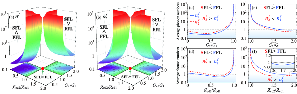
Figure 2: Steady-state mean thermal phonon numbers (a) $n_{1}^{f}$ and (b) $n_{2}^{f}$ in two vibrational modes as functions of the effective optomechanical-coupling ratio $G_{2}/G_{1}$ and the feedback-gain ratio $g_{\mathrm{cd2}}/g_{\mathrm{cd1}}$ of the two vibrational modes, when the system operates with the AMC (i.e., $\tilde{\mu}/\omega_{m}=0.02$). Here the red disks denote the case of SFL$=$FFL, i.e., $g_{\mathrm{cd},2}=g_{\mathrm{cd},1}$ and $G_{2}=G_{1}$. When the strength of the second feedback loop is smaller (larger) than that of the first one [i.e., SFL$<$FFL (SFL$>$FFL)], $n_{1}^{f}$ (blue solid curves) and $n_{2}^{f}$ (red dashed curves) versus (c,e) $G_{2}/G_{1}$ and (d,f) $g_{\mathrm{cd2}}/g_{\mathrm{cd1}}$. Note that SFL$<$FFL (SFL$>$FFL) describes the parameter conditions: $g_{\mathrm{cd}2}<g_{\mathrm{cd}1}$ and $G_{2}<G_{1}$ ($g_{\mathrm{cd}2}>g_{\mathrm{cd}1}$ and $G_{2}>G_{1}$). Here the parameters used are : for (c) $g_{\mathrm{cd1}}=1$ and $g_{\mathrm{cd2}}=0.6$, (d) $G_{\mathrm{1}}=0.4\omega_{1}$ and $G_{\mathrm{2}}=0.7G_{1}$, (e) $g_{\mathrm{cd1}}=1$ and $g_{\mathrm{cd2}}=1.7$, and (f) $G_{\mathrm{1}}=0.4\omega_{1}$ and $G_{\mathrm{2}}=1.8G_{1}$. The inset in (f) is a zoomed-in plot of $n^{f}_{1}$ as a function of $g_{\mathrm{cd2}}/g_{\mathrm{cd1}}$, which clearly shows the dependence of $n^{f}_{1}$ on $g_{\mathrm{cd2}}/g_{\mathrm{cd1}}$. Other parameters are the same as those in Fig.1.

To further illustrate the underlying physics of the multimode refrigeration under the AMC mechanism, we plot the net-refrigeration rate $\gamma_{j,\text{C}}$ of the $j$th vibrational mode versus the AMC strength $\tilde{u}$ at the resonance $\omega=\omega_{m}$, as shown in Fig. 1(c). We find that when turning off the AMC (i.e., $\tilde{u}=0$), the net-refrigeration rates are extremely small (i.e., $\gamma_{j,\mathrm{C}}\approx\gamma_{j}$). These results indicate that all the vibrational modes cannot be cooled when the AMC is absent, i.e., $\tilde{u}=0$. However, when we turn on the AMC (i.e., $\tilde{u}\neq 0$), the net-refrigeration rates $\gamma_{j,\text{C}}$ are giantly enhanced with the increase of the AMC strength $\tilde{u}$. For example, the net-refrigeration rates $\gamma_{j,\mathrm{C}}$ can be increased from $\gamma_{j,\mathrm{C}}/\gamma_{j}\approx 1$ to more than $10^{6}$ in our simulations.

IV.3 Dependence of the multimode optomechanical cooling on the system parameters

In cavity optomechanics, the cold-damping feedback refrigeration of a single vibrational mode can be achieved using the cold-damping effect, which employs a designed feedback force applied to this vibrational mode, and this leads to the freezing of their thermal fluctuations Mancini1998PRL ; Genes2008PRA ; Steixner2005PRA ; Bushev2006PRL ; Rossi2017PRL ; Rossi2018Nature ; Conangla2019PRL ; Tebbenjohanns2019PRL ; Sommer2019PRL ; Guo2019PRL ; Sommer2020PRR . Correspondingly, in principle, the feedback refrigeration of multiple vibrational modes can also be realized based on this feedback-cooling mechanism.

However, in contrast to this anticipation, we find that by using this feedback refrigeration mechanism, a counterintuitive cooling phenomenon emerges, i.e., the multiple vibrational modes cannot be cooled. Physically, the dark mode, which is induced by the coupling of the multiple vibrational modes to a common optical mode, cuts off the thermal-phonon extraction channels. Since the dark mode leads to this counterintuitive uncooling phenomenon, it is natural to ask the question whether one can remove this dark mode to further cool these vibrational modes to their quantum ground states. To this end, the AMC is introduced to our system for removing the dark mode and controlling the refrigeration performance of these vibrational modes.

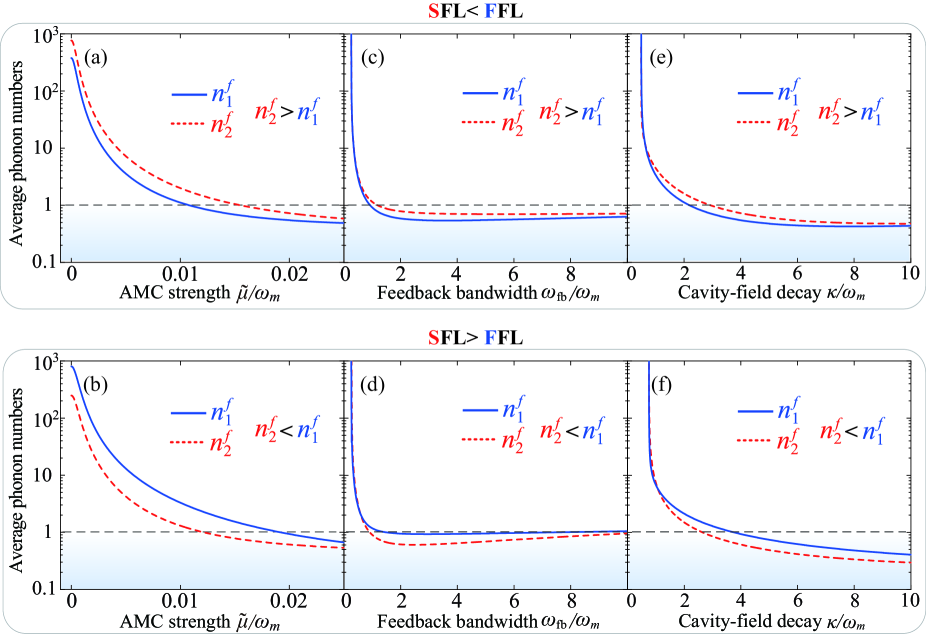
Figure 3: Steady-state mean thermal occupations $n_{1}^{f}$ (blue solid curves) and $n_{2}^{f}$ (red dashed curves) versus: (a, b) the AMC strength $\tilde{u}$, (c,d) the feedback bandwidth $\omega_{\mathrm{fb}}$, and (e,f) the cavity-field decay rate $\kappa$, for the cases when SFL$<$FFL and SFL$>$FFL. Other parameters are the same as those in Fig. 2

Specifically, when the AMC is on, we plotted the steady-state mean phonon numbers $n^{f}_{1}$ and $n^{f}_{2}$ versus the optomechanical-coupling-strength ratio $G_{2}/G_{1}$ and the feedback-gain ratio $g_{\mathrm{cd},2}/g_{\mathrm{cd},1}$ of the two vibrational modes, as shown in Figs. 2(a) and 2(b). It is seen that the two vibrational modes can be efficiently cooled to their quantum ground states ($n^{f}_{1}<1$, $n^{f}_{2}<1$), when the system operates in the regimes for SFL$<$FFL (i.e., $g_{\mathrm{cd},2}<g_{\mathrm{cd},1}$ and $G_{2}<G_{1}$) or SFL$>$FFL (i.e., $g_{\mathrm{cd},2}>g_{\mathrm{cd},1}$ and $G_{2}>G_{1}$). In contrast to the above ground-state refrigeration results, we find that when SFL$=$FFL (i.e., $g_{\mathrm{cd},2}=g_{\mathrm{cd},1}$ and $G_{2}=G_{1}$, see the red disks), the two vibrational modes are not cooled. The physical origin behind this no cooling phenomenon is due to the dark mode, which decouples from the system and prevents the extraction of the phonons. These results mean that the simultaneous ground-state refrigeration of these vibrational modes is achievable owing to the breaking of the system symmetry by introducing the AMC. Breaking the system symmetry leads to the removing of the dark mode.

To further elucidate how the refrigeration performance of the two vibrational modes depends on the parameters of the SFL and FFL, we plot $n^{f}_{1}$ and $n^{f}_{2}$ versus $G_{2}/G_{1}$ [see Figs. 2(c) and 2(e)] and $g_{\mathrm{cd},2}/g_{\mathrm{cd},1}$ [see Figs. 2(d) and 2(f)]. We can see from Figs. 2(c) and 2(d) that when SFL$<$FFL (i.e., $g_{\mathrm{cd},2}<g_{\mathrm{cd},1}$ and $G_{2}<G_{1}$), these mechanical modes can be cooled effectively, and that the refrigeration performance of the first vibrational mode is better than that of the second one. Correspondingly, when SFL$>$FFL (i.e., $g_{\mathrm{cd},2}>g_{\mathrm{cd},1}$ and $G_{2}>G_{1}$), the simultaneous ground-state refrigeration of these vibrational modes can also be realized, and the cooling performance of the second vibrational mode is better than that of the first one. Physically, the strength of the feedback loop directly governs the feedback cooling performance, and this means that the larger is the feedback-loop strength of the resonator, the better is the cooling efficiency of this resonator.

Since the AMC plays a key role in removing the dark mode and achieving the simultaneous refrigeration of the two vibrational modes, the effect of the AMC on the refrigeration performance should be studied in detail. To this end, we plotted the steady-state mean phonon numbers $n^{f}_{1}$ and $n^{f}_{2}$ as functions of the AMC strength $\tilde{u}$ when SFL$>$FFL and SFL$<$FFL, as shown in Figs. 3(a) and 3(b). We find that in the absence of the AMC (i.e., $\tilde{u}=0$), neither of the two vibrational modes can be cooled. In contrast to this, the simultaneous ground-state refrigeration of these vibrational modes is achieved [ i.e., ($n^{f}_{1},n^{f}_{2}<1$)] by introducing the AMC. This is because by employing the AMC, the dark mode can be completely removed and the refrigeration channels of these vibrational modes can be opened.

In addition, in Figs. 3(c) and 3(d), we plot $n_{1}^{f}$ and $n_{2}^{f}$ versus the feedback bandwidth $\omega_{\mathrm{fb}}$, when the AMC is on. We find that the simultaneous ground-sate refrigeration of the two vibrational modes is realized (i.e., $n^{f}_{1},n^{f}_{2}<1$) under the proper parameter conditions, and that the optimal refrigeration of these vibrational modes can be observed for the parameter $\omega_{\mathrm{fb},j}/\omega_{m}>2$. In particular, we demonstrate that, with decreasing the feedback bandwidth, i.e., $\omega_{\mathrm{fb},j}\rightarrow 0$, the refrigeration of the two vibrations becomes inefficient. The physical origin behind this is that a smaller feedback bandwidth corresponds to a longer time delay of the feedback loop, and it leads to a lower cooling efficiency for the vibrational modes.

In particular, we find from in Figs. 3(c) and 3(d) that, when SFL$<$FFL (SFL$>$FFL), the refrigeration performance of the first (second) vibrational mode is better than that of the second (first) one with increasing feedback bandwidth $\omega_{\mathrm{fb},j}$. This asymmetrical cooling is directly induced by the asymmetrical feedback-loop strength, which indicates that the cooling performance is better for a stronger feedback loop.

Furthermore, in Figs. 3(e) and 3(f), the final average phonon numbers $n^{f}_{1}$ and $n^{f}_{2}$ are plotted as a function of the cavity-field decay rate $\kappa$ when SFL$<$FFL and SFL$>$FFL. We see that when we decrease the cavity-field decay rate $\kappa$, the refrigeration performance of the two vibrational modes becomes much worse in the resolved-sideband regimes (i.e., $\kappa/\omega_{m}\ll 1$). However, by increasing $\kappa$, these vibrational modes are efficiently cooled to their quantum ground states (i.e., $n^{f}_{1},n^{f}_{2}<1$), beyond the resolved-sideband regimes: $\kappa/\omega_{m}>1$. In addition, the optimal refrigeration can be observed for $\kappa/\omega_{m}\geqslant 4$. These unresolved-sideband refrigerations are fundamentally different from those in the sideband cooling, for which the optimal cooling is reached only in the resolved-sideband regime Wilson-Rae2007PRL ; Marquardt2007PRL ; Teufel2011Nature .

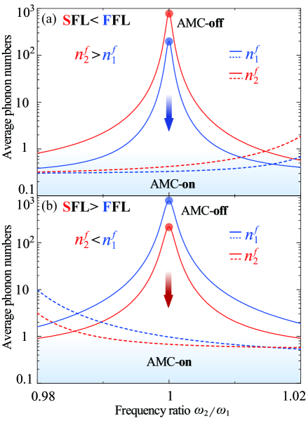
Figure 4: Steady-state mean phonon numbers $n_{1}^{f}$ (blue curves) and $n_{2}^{f}$ (red curves) as a function of the frequency ratio $\omega_{2}/\omega_{1}$ of the two vibrational modes, without ($\tilde{\mu}=0$, solid curves) and with ($\tilde{\mu}=0.02\omega_{1}$, dashed curves) the AMC. The parameters used for (a) are: $g_{cd2}=0.5$ and $G_{2}=0.5G_{1}$, and for (b) are: $g_{cd2}=1.9$ and $G_{2}=1.9G_{1}$. Other parameters are set as Fig. 1.

We find that, surprisingly, the dark-mode effect can also cause a cooling suppression for the near-degenerate-vibration case. To see the width of the frequency-detuning window associated with this dark-mode effect, in Fig. 4 we plotted $n_{1}^{f}$ and $n_{2}^{f}$ versus the ratio $\omega_{2}/\omega_{1}$ without (i.e., $\tilde{u}=0$) and with (i.e., $\tilde{u}/\omega_{1}=0.02$) the AMC. We find that without the AMC, the simultaneous ground-state refrigeration of the two vibrational modes is unfeasible in the frequency-detuning range $0.98<\omega_{2}/\omega_{1}<1.02$. However, when the AMC is turned on, the simultaneous ground-state cooling can be realized in the corresponding region. Our findings mean that the AMC mechanism can lead to the simultaneous ground-state refrigeration of both near-degenerate and degenerate vibrational modes. In particular, when SFL$<$FFL (SFL$>$FFL), the cooling efficiency of the first (second) vibrational mode is better than that of the second (first) one. This is because the cooling is governed by the feedback loop, and the cooling performance is better for a larger feedback loop.

V Discussion and conclusion

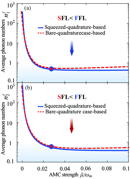
Figure 5: Steady-state average phonon numbers (a) $n^{f}_{1}$ and (b) $n^{f}_{2}$ are plotted as a function of the AMC $\tilde{\mu}$ for the cooling cases of the squeezed (blue solid curves) and bare (red dashed curves) quadratures, under SFL$<$FFL. Here the bare- and squeezed-quadrature-based cases are, respectively, based on the quadratures in Eqs. (1) and (2).

Here, we present some discussions to compare the cooling performance based on both bare and squeezed quadratures. It is obvious that the quadratures $q_{j}$ and $p_{j}$ in Eq. (2) are squeezed with respect to the bare quadratures, and that our present cooling pertains to the squeezed quadratures. Due to the fact that the anti-squeezing may have an effect on phonon number, it is worth to further discuss the cooling results in the bare-quadrature-based case. To this end, we plot the final mean phonon numbers $n^{f}_{j}$ as a function of the AMC strength $\tilde{\mu}$ in both bare- and squeezed-quadrature-based cases, as shown in Figs. 5(a) and 5(b). Here, the blue solid curves show the cooling results in the squeezed-quadrature-based case, while the red dashed curves correspond to that in the bare-quadrature-based case. We find that the two mechanical resonators can be simultaneously cooled to their quantum ground states by introducing the AMC. Physically, the introduced AMC offers an effective strategy to remove the dark mode and, in turn, to rebuild cooling channels for extracting thermal phonons stored in the dark mode. This implies that no actual cooling is observed for the two mechanical resonators when $\tilde{\mu}=0$.

Moreover, we find that when $\tilde{\mu}/\omega_{m}\leqslant 0.025$, an excellent agreement is observed between the bare-quadrature-based (red dashed curves) and squeezed-quadrature-based (blue solid curves) cooling results, i.e., the cooling performances in both bare- and squeezed-quadrature cases are approximately the same in the region $\tilde{\mu}/\omega_{m}\leqslant 0.025$. This can be explained that a weaker AMC strength leads to a smaller squeezing effect with respect to the bare quadratures. In the region $\tilde{\mu}/\omega_{m}>0.025$, the cooling performance of the bare-quadrature-based case becomes worse, while that of the squeezed-quadrature-based case becomes better with increasing $\tilde{\mu}$. Physically, by increasing the AMC strength, the quadratures $q_{j}$ and $p_{j}$ in Eq. (2) are significantly squeezed with respect to the bare quadratures, and, thus, the cooling performance in the squeezed-quadrature-based case can be improved. These results mean that, when the AMC strength $\tilde{\mu}$ is properly chosen (i.e., $\tilde{\mu}/\omega_{m}\leqslant 0.025$), the squeezing effect caused by the AMC has a little effect on cooling performance. However, when $\tilde{\mu}/\omega_{m}>0.025$, the difference of the cooling results in the bare- and squeezed-quadrature-based cases cannot be neglected owing to a significant squeezing effect. Namely, the squeezed-quadrature-based cooling is more efficient than that with the bare quadratures for larger values of the AMC strength, but the differences between these two cases are negligible if the strength is $\tilde{\mu}/\omega_{m}\leqslant 0.025$. Note that in our other simulations, we set $\tilde{\mu}/\omega_{m}=0.02<0.025$, and this indicates that squeezed-quadrature-based cooling can be used to implement bare-quadrature-based cooling when $\tilde{\mu}/\omega_{m}\leqslant 0.025$.

In summary, we proposed a method to achieve the simultaneous ground-state refrigeration of multiple vibrational modes beyond the resolved-sideband regime, and to realize a giant amplification in the net-refrigeration rates. This is realized by introducing an AMC to break the symmetry of the system and, then, it leads to removing the dark-mode effect. By fully analytical treatments, we showed that when the AMC is switched on, the amplification of the net-refrigeration rates can be observed for more than six orders of magnitude. Remarkably, we reveal that without the AMC, the simultaneous ground-state refrigeration of the two vibrational modes is unfeasible; while with the AMC, these vibrational modes can be efficiently cooled to their quantum ground states. Our work could potentially be used for observing quantum mechanical effects and controlling macroscopic mechanical coherence in the unresolved-sideband regime.

*

Appendix A Calculation of the steady-state mean phonon numbers

In this Appendix, we show the remaining expressions of the parameters used in the Eqs. (27)-(35). These expressions are defined as:

$$A_{1}= \omega(\kappa+\omega_{\mathrm{fb}}),A_{2}=\kappa\omega_{\mathrm{fb}}-\omega^{2},A_{3}=\omega(\gamma_{2}\omega^{2}-\kappa\Delta_{2}),A_{4}=\omega^{2}(\gamma_{2}\kappa+\Delta_{2}),$$

$$A_{5}= \omega\omega_{\mathrm{fb}}(\gamma_{2}\kappa-\omega^{2}),A_{6}=\omega^{2}\omega_{\mathrm{fb}}(\gamma_{2}+\kappa),A_{7}=G_{2}g_{\mathrm{cd2}}\omega\omega_{2}\omega_{\mathrm{fb}},A_{8}=\omega\omega_{2}^{2}\omega_{\mathrm{fb}},A_{9}=\kappa\omega_{2}^{2}\omega_{\mathrm{fb}},$$

$$W_{1}= \omega(\gamma_{1}\omega^{2}-\kappa\Delta_{1}),W_{2}=\omega^{2}(\gamma_{1}\kappa+\Delta_{1}),W_{3}=\omega\omega_{\mathrm{fb}}(\gamma_{1}\kappa-\omega^{2}),W_{4}=\omega^{2}\omega_{\mathrm{fb}}(\gamma_{1}+\kappa),$$

$$W_{5}= G_{1}g_{\mathrm{cd1}}\omega\omega_{1}\omega_{\mathrm{fb}},W_{6}=\omega\omega_{1}^{2}\omega_{\mathrm{fb}},W_{7}=\kappa\omega_{1}^{2}\omega_{\mathrm{fb}},B_{1}=A_{1}A_{3}-A_{2}A_{4},$$

$$B_{2}= A_{2}A_{3}+A_{1}A_{4},B_{3}=A_{1}A_{5}+A_{2}A_{6}+A_{1}A_{7}+A_{1}A_{8}-A_{2}A_{9},$$

$$B_{4}= A_{2}A_{5}-A_{1}A_{6}+A_{2}A_{7}+A_{2}A_{8}+A_{1}A_{9},C_{1}=B_{1}-B_{3},$$

$$C_{2}= B_{2}-B_{4},D_{1}=2\tilde{\mu}A_{1}-G_{2}g_{\mathrm{cd1}}\omega\omega_{\mathrm{fb}},D_{2}=2\tilde{\mu}A_{1}-G_{1}g_{\mathrm{cd2}}\omega\omega_{\mathrm{fb}},D_{3}=2\tilde{\mu}A_{2},$$

$$E_{j}= C_{1}D_{1}D_{j+1}+D_{2}D_{3}C_{3-j}+(-1)^{j}(D_{3}^{2}C_{j}-C_{2}D_{1}D_{4-j}),$$

$$Y_{j}= L_{j}-L_{j+2},L_{j}=A_{j}W_{1}+(-1)^{j}A_{3-j}W_{2},$$

$$F_{j}= \omega_{j}\omega_{\mathrm{fb}}x^{2}y^{2}[\gamma_{3-j}^{2}\omega^{2}(\omega^{2}-\kappa\omega_{\mathrm{fb}})$$

$$-G_{3-j}g_{\mathrm{cd(3-j)}}\gamma_{3-j}\omega^{2}\omega_{3-j}\omega_{\mathrm{fb}}+\Delta_{3-j}^{2}(\omega^{2}-\kappa\omega_{\mathrm{fb}})],$$

$$T_{j}= D_{j+1}D_{1}Y_{1}+(-1)^{j}D_{3}^{2}Y_{j}+(-1)^{j+1}D_{1}Y_{2}D_{4-j}+D_{2}D_{3}Y_{3-j},$$ (36)

$$E_{j+2}= \omega_{1}[E_{j}\omega_{2}(A_{1}^{2}+A_{2}^{2})+(-1)^{j+1}A_{j}G_{1}g_{\mathrm{cd1}}\omega\omega_{\mathrm{fb}}(C_{1}^{2}+C_{2}^{2})],L_{j+2}=A_{j}(W_{3}+W_{5}+W_{6})+(-1)^{j+1}A_{3-j}(W_{4}-W_{7}),$$

$$F_{j+2}= \omega_{1}\omega_{2}x^{2}y^{2}\{[-(G_{2}g_{\mathrm{cd1}}+G_{1}g_{\mathrm{cd2}})\omega^{2}+2G_{3-j}g_{\mathrm{cd(3-j)}}\tilde{\mu}\omega_{3-j}+(G_{2}g_{\mathrm{cd1}}+G_{1}g_{\mathrm{cd2}})\omega_{3-j}^{2}]\omega_{\mathrm{fb}}(\omega^{2}-\kappa\omega_{\mathrm{fb}})$$

$$+\gamma_{3-j}[(G_{2}g_{\mathrm{cd1}}+G_{1}g_{\mathrm{cd2}})\omega^{2}\omega_{\mathrm{fb}}(\kappa+\omega_{\mathrm{fb}})-2\tilde{\mu}xy]\},$$

$$T_{j+2}= \omega_{2}[T_{j}\omega_{1}(A_{1}^{2}+A_{2}^{2})+(-1)^{j+1}A_{j}G_{2}g_{\mathrm{cd2}}\omega\omega_{\mathrm{fb}}(Y_{1}^{2}+Y_{2}^{2})],N_{1}=\omega_{2}^{2}f_{+}f_{-},f_{\pm}=2\tilde{\mu}(\kappa\pm i\omega)(\omega\mp i\omega_{\mathrm{fb}})-G_{2}g_{\mathrm{cd1}}\omega\omega_{\mathrm{fb}},$$

$$N_{2}= \omega^{2}x[\gamma_{2}^{2}\omega^{2}+\Delta_{2}^{2}]-2G_{2}g_{\mathrm{cd2}}\omega^{2}\omega_{2}\omega_{\mathrm{fb}}[\omega^{2}\gamma_{2}-\kappa\Delta_{2}]+\{\gamma_{2}^{2}\omega^{2}x+2G_{2}g_{\mathrm{cd2}}\gamma_{2}\kappa\omega^{2}\omega_{2}$$

$$+\kappa^{2}\Delta_{2}^{2}+[\omega^{3}-\omega\omega_{2}(G_{2}g_{\mathrm{cd2}}+\omega_{2})]^{2}\}\omega_{\mathrm{fb}}^{2},$$

$$N_{3}= 4g_{\mathrm{cd2}}^{2}\tilde{\mu}^{2}\omega_{2}^{2}+4g_{\mathrm{cd1}}g_{\mathrm{cd2}}\tilde{\mu}\omega_{2}\Delta_{2}+g_{\mathrm{cd1}}^{2}[\gamma_{2}^{2}\omega^{2}+\Delta_{2}^{2}],N_{4}=(G_{2}\omega_{2}x_{+}+y_{-})(G_{2}\omega_{2}x_{-}+y_{+}),$$

$$x_{\pm}= \omega(G_{2}g_{\mathrm{cd1}}-G_{1}g_{\mathrm{cd2}})/(\kappa\pm i\omega),y_{\pm}=(\omega\mp i\omega_{\mathrm{fb}})[G_{1}\omega(\omega\mp i\gamma_{2})-2G_{2}\tilde{\mu}\omega_{2}-G_{1}\omega_{2}^{2}]/\omega_{\mathrm{fb}},M_{1}=\omega_{1}^{2}w_{+}w_{-},$$

$$M_{2}= \omega^{2}(\kappa^{2}+\omega^{2})[\gamma_{1}^{2}\omega^{2}+\Delta_{1}^{2}]-2G_{1}g_{\mathrm{cd1}}\omega^{2}\omega_{1}\omega_{\mathrm{fb}}[\omega^{2}\gamma_{1}-\kappa\Delta_{1}]+\omega_{\mathrm{fb}}^{2}\{\gamma_{1}^{2}\omega^{2}x+2G_{1}g_{\mathrm{cd1}}\gamma_{1}\kappa\omega^{2}\omega_{1}$$

$$+\kappa^{2}\Delta_{1}^{2}+[\omega^{3}-\omega\omega_{1}(G_{1}g_{\mathrm{cd1}}+\omega_{1})]^{2}\},~{}~{}w_{\pm}=2\tilde{\mu}(\kappa\pm i\omega)(\omega\mp i\omega_{\mathrm{fb}})-G_{1}g_{\mathrm{cd2}}\omega\omega_{\mathrm{fb}},$$

$$M_{3}= 4g_{\mathrm{cd1}}^{2}\tilde{\mu}^{2}\omega_{1}^{2}+4g_{\mathrm{cd1}}g_{\mathrm{cd2}}\tilde{\mu}\omega_{1}\Delta_{1}+g_{\mathrm{cd2}}^{2}[\gamma_{1}^{2}\omega^{2}+\Delta_{1}^{2}],$$

$$M_{4}= (G_{1}\omega_{1}x_{+}+z_{-})(G_{1}\omega_{1}x_{-}+z_{+}).~{}~{}z_{\pm}=(\omega\pm i\omega_{\mathrm{fb}})[2G_{1}\tilde{\mu}\omega_{1}+G_{2}(\Delta_{1}\mp i\gamma_{1}\omega)]/\omega_{\mathrm{fb}},$$

where $j=1,2$, $\Delta_{j}=\omega_{j}^{2}-\omega^{2}$, $\Delta_{3-j}=\omega_{3-j}^{2}-\omega^{2}$, $x=\kappa^{2}+\omega^{2}$, and $y=\omega_{\mathrm{fb}}^{2}+\omega^{2}$.

References

- (1) W. P. Bowen and G. J. Milburn, Quantum Optomechanics (CRC Press, Boca Raton, 2015).
- (2) T. J. Kippenberg and K. J. Vahala, Cavity Optomechanics: Back-Action at the Mesoscale, Science 321, 1172 (2008).
- (3) P. Meystre, A short walk through quantum optomechanics, Ann. Phys. (Berlin) 525, 215 (2013).
- (4) M. Aspelmeyer, T. J. Kippenberg, and F. Marquardt, Cavity optomechanics, Rev. Mod. Phys. 86, 1391 (2014).
- (5) P. Rabl, Photon Blockade Effect in Optomechanical Systems, Phys. Rev. Lett. 107, 063601 (2011).
- (6) A. Nunnenkamp, K. Børkje, and S. M. Girvin, Single-Photon Optomechanics, Phys. Rev. Lett. 107, 063602 (2011).
- (7) J.-Q. Liao, H. K. Cheung, and C. K. Law, Spectrum of single-photon emission and scattering in cavity optomechanics, Phys. Rev. A 85, 025803 (2012).
- (8) J.-Q. Liao and C. K. Law, Correlated two-photon scattering in cavity optomechanics, Phys. Rev. A 87, 043809 (2013).
- (9) J.-Q. Liao and F. Nori, Photon blockade in quadratically coupled optomechanical systems, Phys. Rev. A 88, 023853 (2013).
- (10) F. Zou, D.-G. Lai, and J.-Q. Liao, Enhancement of photon blockade effect via quantum interference, Opt. Express 28, 16175 (2020).
- (11) D. Vitali, S. Gigan, A. Ferreira, H. R. Böhm, P. Tombesi, A. Guerreiro, V. Vedral, A. Zeilinger, and M. Aspelmeyer, Optomechanical Entanglement between a Movable Mirror and a Cavity Field, Phys. Rev. Lett. 98, 030405 (2007).
- (12) G. S. Agarwal and S. Huang, Electromagnetically induced transparency in mechanical effects of light, Phys. Rev. A 81, 041803(R) (2010).
- (13) C. Genes, H. Ritsch, M. Drewsen, and A. Dantan, Atom-membrane cooling and entanglement using cavity electromagnetically induced transparency, Phys. Rev. A 84, 051801(R) (2011).
- (14) Y.-D. Wang and A. A. Clerk, Reservoir-Engineered Entanglement in Optomechanical Systems, Phys. Rev. Lett. 110, 253601 (2013).
- (15) Y.-C. Liu, Y.-F. Xiao, Y.-L. Chen, X.-C. Yu, and Q. Gong, Parametric Down-Conversion and Polariton Pair Generation in Optomechanical Systems, Phys. Rev. Lett. 111, 083601 (2013).
- (16) X.-W. Xu and Y. Li, Optical nonreciprocity and optomechanical circulator in three-mode optomechanical systems, Phys. Rev. A 91, 053854 (2015).
- (17) B. P. Hou, L. F. Wei, and S. J. Wang, Optomechanically induced transparency and absorption in hybridized optomechanical systems, Phys. Rev. A 92, 033829 (2015).
- (18) C. Bai, B. P. Hou, D.-G. Lai, and D. Wu, Tunable optomechanically induced transparency in double quadratically coupled optomechanical cavities within a common reservoir, Phys. Rev. A 93, 043804 (2016).
- (19) Q. Yang, B. P. Hou, and D.-G. Lai, Local modulation of double optomechanically induced transparency and amplification, Opt. Express textbf25(9), 009697 (2017).
- (20) D.-G. Lai, X. Wang, W. Qin, B.-P. Hou, F. Nori, and J.-Q. Liao, Tunable optomechanically induced transparency by controlling the dark-mode effect, Phys. Rev. A 102, 023707 (2020).
- (21) H. Xu, D.-G. Lai, Y.-B. Qian, B.-P. Hou, A. Miranowicz, and F. Nori, Optomechanical dynamics in the PT- and broken-PT-symmetric regimes, Phys. Rev. A 104, 053518 (2021).
- (22) Y.-B. Qian, D.-G. Lai, M.-R. Chen, and B.-P. Hou, Nonreciprocal photon transmission with quantum noise reduction via cross-Kerr nonlinearity, Phys. Rev. A 104, 033705 (2021).
- (23) M. Cirio, K. Debnath, N. Lambert, and F. Nori, Amplified Optomechanical Transduction of Virtual Radiation Pressure, Phys. Rev. Lett. 119, 053601 (2017).
- (24) X.-Y. Lü, L.-L. Zheng, G.-L. Zhu, and Y. Wu, Single-Photon-Triggered Quantum Phase Transition, Phys. Rev. Applied 9, 064006 (2018).
- (25) S. Zippilli, N. Kralj, M. Rossi, G. D. Giuseppe, and D. Vitali, Cavity optomechanics with feedback-controlled in-loop light, Phys. Rev. A 98, 023828 (2018).
- (26) W. Qin, V. Macrì, A. Miranowicz, S. Savasta, and F. Nori, Emission of photon pairs by mechanical stimulation of the squeezed vacuum, Phys. Rev. A 100, 062501 (2019).
- (27) H. Wang, X. Gu, Y.-X. Liu, A. Miranowicz, and F. Nori, Tunable photon blockade in a hybrid system consisting of an optomechanical device coupled to a two-level system, Phys. Rev. A 92, 033806 (2015).
- (28) B. Li, R. Huang, X.-W. Xu, A. Miranowicz, and H. Jing, Nonreciprocal unconventional photon blockade in a spinning optomechanical system, Phot. Res. 7, 630-641 (2019).
- (29) Y.-F. Jiao, Y. -L. Zhang, A. Miranowicz, L. -M. Kuang, and H. Jing, Nonreciprocal Quantum Entanglement Against Backscattering, Phys. Rev. Lett. 125, 143605 (2020).
- (30) I. Wilson-Rae, N. Nooshi, W. Zwerger, and T. J. Kippenberg, Theory of Ground State Cooling of a Mechanical Oscillator Using Dynamical Backaction, Phys. Rev. Lett. 99, 093901 (2007).
- (31) F. Marquardt, J. P. Chen, A. A. Clerk, and S. M. Girvin, Quantum Theory of Cavity-Assisted Sideband Cooling of Mechanical Motion, Phys. Rev. Lett. 99, 093902 (2007).
- (32) C. Genes, D. Vitali, P. Tombesi, S. Gigan, and M. Aspelmeyer, Ground-state cooling of a micromechanical oscillator: Comparing cold damping and cavity-assisted cooling schemes, Phys. Rev. A 77, 033804 (2008).
- (33) J. Chan, T. P. Alegre, A. H. Safavi-Naeini, J. T. Hill, A. Krause, S. Groeblacher, M. Aspelmeyer, and O. Painter, Laser cooling of a nanomechanical oscillator into its quantum ground state, Nature (London) 478, 89 (2011).
- (34) J. D. Teufel, T. Donner, D. Li, J. W. Harlow, M. S. Allman, K. Cicak, A. J. Sirois, J. D. Whittaker, K. W. Lehnert, and R. W. Simmonds, Sideband cooling of micromechanical motion to the quantum ground state, Nature (London) 475, 359 (2011).
- (35) J. B. Clark, F. Lecocq, R. W. Simmonds, J. Aumentado, and J. D. Teufel, Sideband cooling beyond the quantum backaction limit with squeezed light, Nature (London) 541, 191 (2017).
- (36) S. Mancini, D. Vitali, and P. Tombesi, Optomechanical Cooling of a Macroscopic Oscillator by Homodyne Feedback, Phys. Rev. Lett. 80, 688 (1998).
- (37) V. Steixner, P. Rabl, and P. Zoller, Quantum feedback cooling of a single trapped ion in front of a mirror, Phys. Rev. A 72, 043826 (2005).
- (38) P. Bushev, D. Rotter, A. Wilson, F. M. C. Dubin, C. Becher, J. Eschner, R. Blatt, V. Steixner, P. Rabl, and P. Zoller, Feedback Cooling of a Single Trapped Ion, Phys. Rev. Lett. 96, 043003 (2006).
- (39) M. Rossi, N. Kralj, S. Zippilli, R. Natali, A. Borrielli, G. Pandraud, E. Serra, G. D. Giuseppe, and D. Vitali, Enhancing Sideband Cooling by Feedback-Controlled Light, Phys. Rev. Lett. 119, 123603 (2017).
- (40) M. Rossi, D. Mason, J. Chen, Y. Tsaturyan, and A. Schliesser, Measurement-based quantum control of mechanical motion, Nature (London) 563, 53 (2018).
- (41) G. P. Conangla, F. Ricci, M. T. Cuairan, A. W. Schell, N. Meyer, and R. Quidant, Optimal Feedback Cooling of a Charged Levitated Nanoparticle with Adaptive Control, Phys. Rev. Lett. 122, 223602 (2019).
- (42) F. Tebbenjohanns, M. Frimmer, A. Militaru, V. Jain, and L. Novotny, Cold Damping of an Optically Levitated Nanoparticle to Microkelvin Temperatures, Phys. Rev. Lett. 122, 223601 (2019).
- (43) C. Sommer and C. Genes, Partial Optomechanical Refrigeration via Multimode Cold-Damping Feedback, Phys. Rev. Lett. 123, 203605 (2019).
- (44) J. Guo, R. Norte, and S. Gröblacher, Feedback Cooling of a Room Temperature Mechanical Oscillator close to its Motional Ground State, Phys. Rev. Lett. 123, 223602 (2019).
- (45) C. Sommer, A. Ghosh, and C. Genes, Multimode cold-damping optomechanics with delayed feedback, Phys. Rev. Research 2 033299 (2020).
- (46) H. Xu, D. Mason, L. Jiang, and J. G. E. Harris, Topological energy transfer in an optomechanical system with exceptional points, Nature (London) 537, 80 (2016).
- (47) S. Mancini, V. Giovannetti, D. Vitali, and P. Tombesi, Entangling Macroscopic Oscillators Exploiting Radiation Pressure, Phys. Rev. Lett. 88, 120401 (2002).
- (48) L. Tian and P. Zoller, Coupled Ion-Nanomechanical Systems, Phys. Rev. Lett. 93, 266403 (2004).
- (49) F. Massel, S. U. Cho, J.-M. Pirkkalainen, P. J. Hakonen, T. T. Heikkilä, and M. A. Sillanpää, Multimode circuit optomechanics near the quantum limit, Nat. Commun. 3, 987 (2012).
- (50) A. Mari, A. Farace, N. Didier, V. Giovannetti, and R. Fazio, Measures of Quantum Synchronization in Continuous Variable Systems, Phys. Rev. Lett. 111, 103605 (2013).
- (51) M. H. Matheny, M. Grau, L. G. Villanueva, R. B. Karabalin, M. C. Cross, and M. L. Roukes, Phase Synchronization of Two Anharmonic Nanomechanical Oscillators, Phys. Rev. Lett. 112, 014101 (2014).
- (52) M. Zhang, S. Shah, J. Cardenas, and M. Lipson, Synchronization and Phase Noise Reduction in Micromechanical Oscillator Arrays Coupled through Light, Phys. Rev. Lett. 115, 163902 (2015).
- (53) C. F. Ockeloen-Korppi, E. Damskägg, J.-M. Pirkkalainen, M. Asjad, A. A. Clerk, F. Massel, M. J. Woolley, and M. A. Sillanpää, Stabilized entanglement of massive mechanical oscillators, Nature (London) 556, 478 (2018).
- (54) R. Riedinger, A. Wallucks, I. Marinković, C. Löschnauer, M. Aspelmeyer, S. Hong, and S. Gröblacher, Remote quantum entanglement between two micromechanical oscillators, Nature (London) 556, 473 (2018).
- (55) W. Qin, A. Miranowicz, G. L. Long, J. Q. You, and F. Nori, Proposal to test quantum wave-particle superposition on massive mechanical resonators, npj Quantum Information 5, 58 (2019).
- (56) O. D. Stefano, A. Settineri, V. Macrì, A. Ridolfo, R. Stassi, A. F. Kockum, S. Savasta, and F. Nori, Interaction of Mechanical Oscillators Mediated by the Exchange of Virtual Photon Pairs, Phys. Rev. Lett. 122, 030402 (2019).
- (57) S. Kotler, et al., Direct observation of deterministic macroscopic entanglement, Science 372, 622 (2021).
- (58) L. M. de Lépinay, C. F. Ockeloen-Korppi, M. J. Woolley, and M. A. Sillanpää, Quantum mechanics-free subsystem with mechanical oscillators, Science 372, 625 (2021).
- (59) G. Heinrich, M. Ludwig, J. Qian, B. Kubala, and F. Marquardt, Collective Dynamics in Optomechanical Arrays, Phys. Rev. Lett. 107, 043603 (2011).
- (60) A. Xuereb, C. Genes, and A. Dantan, Strong Coupling and Long-Range Collective Interactions in Optomechanical Arrays, Phys. Rev. Lett. 109, 223601 (2012).
- (61) M. Ludwig and F. Marquardt, Quantum Many-Body Dynamics in Optomechanical Arrays, Phys. Rev. Lett. 111, 073603 (2013).
- (62) A. Xuereb, C. Genes, G. Pupillo, M. Paternostro, and A. Dantan, Reconfigurable Long-Range Phonon Dynamics in Optomechanical Arrays, Phys. Rev. Lett. 112, 133604 (2014).
- (63) A. Xuereb, A. Imparato, and A. Dantan, Heat transport in harmonic oscillator systems with thermal baths: application to optomechanical arrays, New J. Phys. 17, 055013 (2015).
- (64) O. Černotík, S. Mahmoodian, and K. Hammerer, Spatially Adiabatic Frequency Conversion in Optoelectromechanical Arrays, Phys. Rev. Lett. 121, 110506 (2018).
- (65) P. Rabl, S. J. Kolkowitz, F. H. L. Koppens, J. G. E. Harris, P. Zoller, and M. D. Lukin, A quantum spin transducer based on nanoelectromechanical resonator arrays, Nat. Phys. 6, 602 (2010).
- (66) F. Massel, T. T. Heikkilä, J.-M. Pirkkalainen, S. U. Cho, H. Saloniemi, P. J. Hakonen, and M. A. Sillanpää, Microwave amplification with nanomechanical resonators, Nature (London) 480, 351 (2011).
- (67) P. Huang, P. Wang, J. Zhou, Z. Wang, C. Ju, Z. Wang, Y. Shen, C. Duan, and J. Du, Demonstration of Motion Transduction Based on Parametrically Coupled Mechanical Resonators, Phys. Rev. Lett. 110, 227202 (2013).
- (68) P. Huang, L. Zhang, J. Zhou, T. Tian, P. Yin, C. Duan, and J. Du, Nonreciprocal Radio Frequency Transduction in a Parametric Mechanical Artificial Lattice, Phys. Rev. Lett. 117, 017701 (2016).
- (69) S. C. Masmanidis, R. B. Karabalin, I. D. Vlaminck, G. Borghs, M. R. Freeman, and M. L. Roukes, Multifunctional Nanomechanical Systems via Tunably Coupled Piezoelectric Actuation, Science 317, 780 (2007).
- (70) I. Mahboob and H. Yamaguchi, Bit storage and bit flip operations in an electromechanical oscillator, Nat. Nanotechnol. 3, 275 (2008).
- (71) D. Malz, L. D. Tóth, N. R. Bernier, A. K. Feofanov, T. J. Kippenberg, and A. Nunnenkamp, Quantum-Limited Directional Amplifiers with Optomechanics, Phys. Rev. Lett. 120, 023601 (2018).
- (72) Z. Shen, Y.-L. Zhang, Y. Chen, C.-L. Zou, Y.-F. Xiao, X.-B. Zou, F.-W. Sun, G.-C. Guo, and C.-H. Dong, Experimental realization of optomechanically induced non-reciprocity, Nat. Photonics 10, 657 (2016).
- (73) Z. Shen, Y.-L. Zhang, Y. Chen, F.-W. Sun, X.-B. Zou, G.-C. Guo, C.-L. Zou, and C.-H. Dong, Reconfigurable optomechanical circulator and directional amplifier, Nat. Commun. 9, 1797 (2018).
- (74) Z. Shen, Y.-L. Zhang, Y. Chen, Y.-F. Xiao, C.-L. Zou, G.-C. Guo, C.-H. Dong, Non-reciprocal frequency conversion and mode routing in a microresonator, arXiv:2111.07030 (2022).
- (75) K. Fang, J. Luo, A. Metelmann, M. H. Matheny, F. Marquardt, A. A. Clerk, and O. Painter, Generalized non-reciprocity in an optomechanical circuit via synthetic magnetism and reservoir engineering, Nat. Phys. 13, 465 (2017).
- (76) H. Xu, L. Jiang, A. A. Clerk, and J. G. E. Harris, Nonreciprocal control and cooling of phonon modes in an optomechanical system, Nature (London) 568, 65 (2019).
- (77) J. P. Mathew, J. d. Pino, and E. Verhagen, Synthetic gauge fields for phonon transport in a nano-optomechanical system, Nat. Nanotechnol. 15, 198 (2020).
- (78) C. Yang, X. Wei, J. Sheng, and H. Wu, Phonon heat transport in cavity-mediated optomechanical nanoresonators, Nat. Commun. 11, 4656 (2020).
- (79) C. Sanavio, V. Peano, and A. Xuereb, Nonreciprocal topological phononics in optomechanical arrays, Phys. Rev. B 101, 085108 (2020).
- (80) Y.-C. Liu, Y.-F. Xiao, X. Luan, and C. W. Wong, Dynamic Dissipative Cooling of a Mechanical Resonator in Strong Coupling Optomechanics, Phys. Rev. Lett. 110, 153606 (2013)
- (81) Y.-C. Liu, Y.-F. Shen, Q. Gong, and Y.-F. Xiao, Optimal limits of cavity optomechanical cooling in the strong-coupling regime, Phys. Rev. A 89, 053821 (2014).
- (82) X.-T. Wang, S. Vinjanampathy, F. W. Strauch, and K. Jacobs, Ultraefficient Cooling of Resonators: Beating Sideband Cooling with Quantum Control, Phys. Rev. Lett. 107, 177204 (2011).
- (83) Y. Li, L.-A. Wu, Y.-D. Wang, and L.-P. Yang, Nondeterministic ultrafast ground-state cooling of a mechanical resonator, Phys. Rev. B 84, 094502 (2011).
- (84) L.-L. Yan, J.-Q. Zhang, S. Zhang, and M. Feng, Efficient cooling of quantized vibrations using a four-level configuration, Phys. Rev. A 94, 063419 (2016).
- (85) J.-Q. Liao and C. K. Law, Cooling of a mirror in cavity optomechanics with a chirped pulse, Phys. Rev. A 84, 053838 (2011).
- (86) S. Machnes, J. Cerrillo, M. Aspelmeyer, W. Wieczorek, M. B. Plenio, and A. Retzker, Pulsed Laser Cooling for Cavity Optomechanical Resonators, Phys. Rev. Lett. 108, 153601 (2012).
- (87) D.-G. Lai, J.-F. Huang, X.-L. Yin, B.-P. Hou, W. Li, D. Vitali, F. Nori, and J.-Q. Liao, Nonreciprocal ground-state cooling of multiple mechanical resonators, Phys. Rev. A 102, 011502(R) (2020).
- (88) D.-G. Lai, F. Zou, B.-P. Hou, Y.-F. Xiao, and J.-Q. Liao, Simultaneous cooling of coupled mechanical resonators in cavity optomechanics, Phys. Rev. A 98, 023860 (2018).
- (89) D.-G. Lai, J. Huang, B.-P. Hou, F. Nori, and J.-Q. Liao, Domino cooling of a coupled mechanical-resonator chain via cold-damping feedback, Phys. Rev. A 103, 063509 (2021).
- (90) D.-G. Lai, W. Qin, B.-P. Hou, A. Miranowicz, and F. Nori, Significant enhancement in refrigeration and entanglement in auxiliary-cavity-assisted optomechanical systems, Phys. Rev. A 104, 043521 (2021).
- (91) M. Xu, X. Han, C.-L. Zou, W. Fu, Y. Xu, C. Zhong, L. Jiang, and H. X. Tang, Radiative Cooling of a Superconducting Resonator, Phys. Rev. Lett. 124, 033602 (2020).
- (92) L. Qiu, I. Shomroni, P. Seidler, and T. J. Kippenberg, Laser Cooling of a Nanomechanical Oscillator to Its Zero-Point Energy, Phys. Rev. Lett. 124, 173601 (2020).
- (93) F. Xue, Y. D. Wang, Y. X. Liu, and F. Nori, Cooling a micro-mechanical beam by coupling it to a transmission line, Phys. Rev. B 76, 205302 (2007).
- (94) J. Q. You, Y. X. Liu, and F. Nori, Simultaneous cooling of an artificial atom and its neighboring quantum system, Phys. Rev. Lett. 100, 047001 (2008).
- (95) J. Zhang, Y. X. Liu, and F. Nori, Cooling and squeezing the fluctuations of a nanomechanical beam by indirect quantum feedback control, Phys. Rev. A 79, 052102 (2009).
- (96) S. D. Liberato, N. Lambert, and F. Nori, Quantum noise in photothermal cooling, Phys. Rev. A 83, 033809 (2011).
- (97) M. Grajcar, S. Ashhab, J. R. Johansson, and F. Nori, Lower limit on the achievable temperature in resonator-based sideband cooling, Phys. Rev. B 78, 035406 (2008).
- (98) F. Nori, Atomic physics with a circuit, Nat. Physics 4, 589 (2008).
- (99) Z. L. Xiang, S. Ashhab, J. Q. You, and F. Nori, Hybrid quantum circuits: Superconducting circuits interacting with other quantum systems, Rev. Mod. Phys. 85, 623 (2013).
- (100) M. O. Scully and M. S. Zubairy, Quantum Optics (Cambridge University Press, Cambridge, 1997).
- (101) G. S. Agarwal, Quantum Optics (Cambridge University Press, Cambridge, 2013).
- (102) C. Genes, D. Vitali, and P. Tombesi, Simultaneous cooling and entanglement of mechanical modes of a micromirror in an optical cavity, New J. Phys. 10, 095009 (2008).
- (103) A. B. Shkarin, N. E. Flowers-Jacobs, S. W. Hoch, A. D. Kashkanova, C. Deutsch, J. Reichel, and J. G. E. Harris, Optically Mediated Hybridization between Two Mechanical Modes, Phys. Rev. Lett. 112, 013602 (2014).
- (104) M. C. Kuzyk and H. Wang, Controlling multimode optomechanical interactions via interference, Phys. Rev. A 96, 023860 (2017).
- (105) C. F. Ockeloen-Korppi, M. F. Gely, E. Damskägg, M. Jenkins, G. A. Steele, and M. A. Sillanpää, Sideband cooling of nearly degenerate micromechanical oscillators in a multimode optomechanical system, Phys. Rev. A 99, 023826 (2019).
- (106) J. Huang, D.-G. Lai, C. Liu, J.-F. Huang, F. Nori, J.-Q. Liao, Multimode Optomechanical Cooling via General Dark-Mode Control, Phys. Rev. A 106, 013526 (2022).
- (107) J.-Y. Liu, W. Liu, D. Xu, J.-C. Shi, H. Xu, Q. Gong, and Y.-F. Xiao, Ground-state cooling of multiple near-degenerate mechanical modes, Phys. Rev. A 105, 053518 (2022).
- (108) D.-G. Lai, J.-Q. Liao, A. Miranowicz, and F. Nori, Noise-Tolerant Optomechanical Entanglement via Synthetic Magnetism, Phys. Rev. Lett. 129, 063602 (2022).
- (109) D.-G. Lai, W. Qin, A. Miranowicz, and F. Nori, Efficient optomechanical refrigeration of two vibrations via an auxiliary feedback loop: Giant enhancement in mechanical susceptibilities and net cooling rates, Phys. Rev. Research 4, 033102 (2022).
- (110) D.-G. Lai, Y.-H. Chen, W. Qin, A. Miranowicz, and F. Nori, Tripartite optomechanical entanglement via optical-dark-mode control, Phys. Rev. Research 4, 033112 (2022).