Learning Gradient-based Mixup towards Flatter Minima for Domain Generalization

Abstract

To address the distribution shifts between training and test data, domain generalization (DG) leverages multiple source domains to learn a model that generalizes well to unseen domains. However, existing DG methods generally suffer from overfitting to the source domains, partly due to the limited coverage of the expected region in feature space. Motivated by this, we propose to perform mixup with data interpolation and extrapolation to cover the potential unseen regions. To prevent the detrimental effects of unconstrained extrapolation, we carefully design a policy to generate the instance weights, named Flatness-aware Gradient-based Mixup (FGMix). The policy employs a gradient-based similarity to assign greater weights to instances that carry more invariant information, and learns the similarity function towards flatter minima for better generalization. On the DomainBed benchmark, we validate the efficacy of various designs of FGMix and demonstrate its superiority over other DG algorithms.

1 Introduction

The success of machine learning systems relies on the assumption that the training and test data are drawn from the same distribution. However, this i.i.d. assumption does not always hold in real-world applications, e.g., when the training and test data are acquired with different devices or under different conditions. When such distribution shifts occur, the systems may fail to generalize to test data if they learn to rely on the spurious cues for prediction (e.g., texture or backgrounds). 

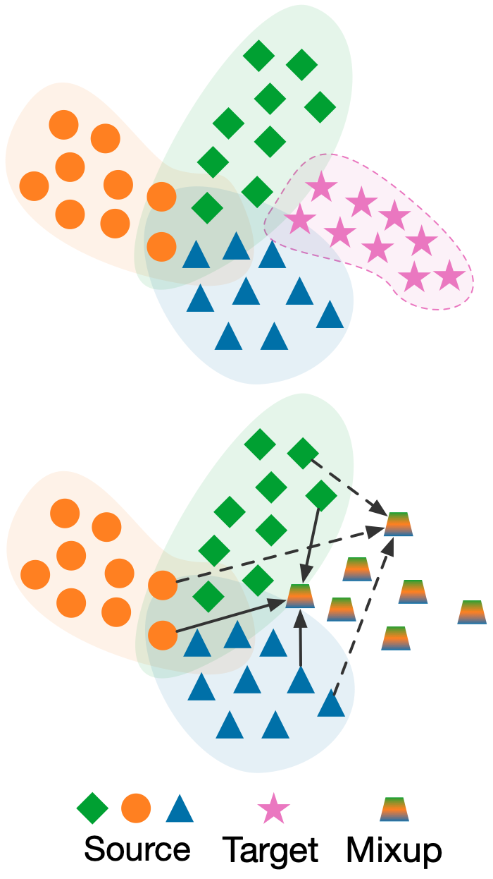
Figure 1: Mixup via interpolation or extrapolation.

Domain generalization (DG) [5, 29, 24, 22] addresses this problem by leveraging data from multiple source domains to train a model that generalizes well to unseen target domain. Existing methods mainly focus on extracting invariant features from source domains or leveraging meta-learning approach to learn a transferable model [29, 24, 23, 2, 25]. Nevertheless, most of the DG methods still suffer from the problem of overfitting to the source domains. As illustrated in Figure 1, the upper subfigure depicts some latent representations of data from multiple domains. The classifier is trained to perform well on the source domains (i.e., diamonds, circles and triangles). If the target domain (i.e., stars) is located at a region that is not covered by the source domains, it is possible that the learned classifier will perform poorly on it. Recently, mixup-based methods are developed to address this issue [46, 42, 27, 49, 43]. Generally, interpolated data are used for model training such that the unseen regions within the convex hull of the source domains will also be covered, as shown by the solid arrows in the lower subfigure of Figure 1. But what if the target domain is located outside of the convex hull? In that case, interpolated data are clearly not sufficient, and one may need to consider data extrapolation, as shown by the dotted arrows.

Data extrapolation is rarely considered in the existing mixup-based methods, probably due to that without proper mixup strategy, extrapolated data may deviate too much from the expected region and become devastating to model training. Hence, unlike the existing methods which simply adopt random weights for mixup, a carefully designed weight generation policy is required to produce meaningful extrapolated data. To begin with, the weight associated with each instance involved in a linear combination should be based on its relations with other instances involved in the same combination - an idea similar to context-aware attention. Inspired by the gradient-based approach for DG [23, 31, 28, 37], which relies on gradient alignment for domain-invariant learning, we propose to compute the relation or similarity between instances based on gradients. Since the gradient similarity indicates how much information are shared between two instances from the perspective of learning, instances with greater sum of similarities with respect to all the other instances in the same combination can be considered as carrying more invariant information, and hence should be assigned greater weights. As a result, the mixup data will absorb a larger portion from the instances containing more invariant features.

To further encourage better generalization of the classifier learned with the mixup data, instead of using a pre-defined similarity metric, we employ a learnable similarity function and optimize it towards flatter minima of the classifier. A flat minimum is defined as a region in loss surface where the loss varies slowly with changes in model parameters [17]. It has long been established that the flatness of a model minimizer is strongly associated with its generalization ability [20, 12, 19]. In the field of DG, Cha et al. [6], Arpit et al. [1] recently demonstrate the importance of seeking flat minima, achieving evident performance gains on the DomainBed benchmark [13].

Different from the existing flatness-aware optimization methods which are designed to search for flat minima in a given loss surface (i.e., based on the original training data), we propose to flatten the loss surface by generating new mixup data - an approach that is orthogonal to the existing flatness-aware solvers. Specifically, we propose to learn the policy of generating instance weights such that the resultant loss surface based on the mixture of original and generated data is flatter. This method can be considered as providing a flatter loss surface for the optimizer to explore, increasing the chance of covering the test optima. Using it jointly with a flatness-aware optimizer further enhances performance, as will be illustrated later. In addition to the flatness-aware learning objective for the generation policy, we further impose an auxiliary adversarial loss to constrain that the generated data conform to a prior distribution for regularization purpose. 

To summarize, we propose a Flatness-aware Gradient-based Mixup (FGMix) method which performs mixup with instance weights based on gradient similarity. A learnable similarity function is optimized towards generating a flatter loss surface for better generalization and encouraged to conform to a prior to avoid over-extrapolation. Through extensive experiments, we validate the efficacy of various designs of FGMix quantitatively and qualitatively, and show that FGMix achieves the state-of-the-art performance on the DomainBed benchmark.

2 Related Work

Mixup-based Methods

Mixup [46] is a data augmentation method that extends the training distribution by linearly interpolating random pairs of examples and labels. Incorporating mixup data for training is equivalent to minimizing the vicinal risk [7] which enables better generalization. Recently, different forms of mixup are developed. Cutmix [45] cuts out a patch from an image and switch it with another image. Remix [9] assigns greater weights to the minority class label to tackle the class imbalance issue. Manifold Mixup [42] performs interpolations at the intermediate layers to enable smoothness in higher-level semantics. Related to our work, MetaMixup [27] and AdaMixup [14] learn the interpolation policy adaptively from data. The former learns by simulating pseudo-target and pseudo-source from the actual source domains, while the latter learns to avoid the “manifold intrusion" issue caused by the conflicts between mixup labels and original labels. Focusing on DG, MixStyle [49] interpolates the feature statistics (known as styles) to synthesize novel domains. Wang et al. [43] adapt mixup to heterogeneous setting where the label spaces are disjoint for source and target. Despite the effectiveness of various mixup methods, they mainly perform interpolation, while our work further explores the potential of data extrapolation to tackle the situation where the distribution shift between source and target is significant.

Gradient-based Methods

Gradients as the update steps for SGD-based optimizers normally lie at the heart of deep learning algorithms. However, learning a single model for multiple tasks or distributions often runs into the problem of gradient interference which can lead to ineffective optimization [35]. In the context of DG, conflicting gradients often correspond to spurious domain-specific information which can be detrimental for learning an invariant model [28]. The first approach to solve gradient conflicts focuses on performing some gradient surgery at each gradient step. PCGrad [44] for multi-task learning projects a task’s gradient onto the normal plane of gradients of other tasks that it has conflicts with. For DG, Mansilla et al. [28], Parascandolo et al. [31] propose to mask out gradient components that have conflicting signs across domains. Shahtalebi et al. [36] further develop a smoothed-out masking method by promoting agreement among the gradient magnitudes as well. The second approach to tackle gradient conflicts typically include gradient alignment in the learning objective. Fish [37] explicitly optimizes the dot product between domain gradients with an efficient first-order algorithm. Fishr [34] further enforces that the variances of gradients are matched across domains. MLDG [23] employs a meta-learning approach where the meta-objective is equivalent to aligning the gradients between pseudo-source and pseudo-target domains. Different from the previous works, here we implicitly perform gradient alignment by assigning greater weights to instances whose gradients have greater overall similarity to the others in the same combination. As a result, the mixup data will contain more invariant information for learning the classifier.

Flatness-aware Optimization

The connection between flatness of minima and generalization has long been established through various theories [20, 17, 26, 8]. Intuitively, a flatter minimum is more robust against shifts in loss landscape between training and test data. In order to find model minimizer with better generalization, algorithms that search for flat minima are developed, which either penalizing sharpness explicitly in the objective function [17, 8, 11] or performing weight averaging to reach the flatter central region of the found minima [18, 15]. The latter has recently been shown to deliver remarkable gains on DG tasks [6, 1]. Orthogonal to the existing methods that search for flat minima, we propose to generate new data to flatten the loss surface, which allows for the optimizer to explore in a wider region where the chance of covering the target domain is higher. We show that when used jointly with weight averaging for variance reduction, our method achieves better results.

3 Methodology

In the DG setting, suppose there are $k$ source domains $\mathcal{S}=\{\mathcal{S}_{1},...,\mathcal{S}_{k}\}$ available for training, and we have the training data $S_{i}=\{(\mathbf{x}_{i,j},y_{i,j})\}_{j=1}^{|S_{i}|}$ drawn from the $i$-th source domain $\mathcal{S}_{i}$. Our goal is to learn a domain-invariant model $f:\mathbf{x}\rightarrow y$ from $S=\{S_{1},...,S_{k}\}$, which generalizes well to an unseen target domain $\mathcal{T}$. We assume the model is formed by two parts: a feature extractor $g_{\theta}$ and a classifier $h_{\phi}$, i.e., $f(\mathbf{x})=h_{\phi}(g_{\theta}(\mathbf{x}))$. Following Berthelot et al. [4], we refer to the data instances projected onto the latent space through $g_{\theta}$ as latent codes, i.e., the latent code of an instance $\mathbf{x}$ is $\mathbf{z}=g_{\theta}(\mathbf{x})$. The classifier is learned on top of the latent codes. Here, we only consider the homogeneous DG setting where the source and target domains share the same label space, i.e., $\mathcal{Y}_{\mathcal{S}_{i}}=\mathcal{Y}_{\mathcal{T}},\forall i\in\{1,...,k\}$. In this case, a single classifier $h_{\phi}$ is learned and shared across domains.

3.1 Latent Code Augmentation

We follow the standard mixup implementation [27] to combine latent codes from multiple domains. Specifically, we sample $k$ instances $\{\mathbf{x}_{1},...,\mathbf{x}_{k}\}$, each from one of the $k$ source domains, and feed them into the feature extractor $g_{\theta}$ to obtain the respective $k$ latent codes $\{\mathbf{z}_{1},...,\mathbf{z}_{k}\}$. A mixup latent code is generated by linearly combining the $k$ latent codes, and the classifier $h_{\phi}$ is learned to optimize the combined loss of the $k$ labels $\{y_{1},...,y_{k}\}$ associated with the $k$ instances. Formally, given the linear weights $\{a_{1},...,a_{k}\}$ where $\sum_{i=1}^{k}a_{i}=1$, the newly generated latent code $\mathbf{z}_{new}$ and the corresponding loss $l_{new}$ are obtained by:

$$\mathbf{z}_{new}=\sum_{i=1}^{k}a_{i}\mathbf{z}_{i},\ \ \ l_{new}=\sum_{i=1}^{k}a_{i}l(y_{i},h_{\phi}(\mathbf{z}_{new})).\$$ (1)

To allow for both interpolation and extrapolation to occur, here we do not enforce positivity constraint on $a_{i}$. Note that when $0\leq a_{i}\leq 1$ for all $i\in\{1,...,k\}$, the generated $\mathbf{z}_{new}$ is an interpolation (i.e., within the convex hull formed by $\{\mathbf{z}_{1},...,\mathbf{z}_{k}\}$), and when $a_{i}<0$ for any $i\in\{1,...,k\}$, the generated $\mathbf{z}_{new}$ is an extrapolation (i.e., outside the convex hull formed by $\{\mathbf{z}_{1},...,\mathbf{z}_{k}\}$).

The generated latent codes are used together with the original latent codes to train the classifier $h_{\phi}$. The feature extractor $g_{\theta}$ is also trained jointly to learn the domain-invariant, discriminative latent representations. Formally, suppose $n$ instances are generated from mixup, the model parameters $\{\theta,\phi\}$ are optimized by the following objective:

$$\mathop{\min}_{\theta,\phi}\frac{1}{|S|+n}\left(\sum_{i=1}^{k}\sum_{j=1}^{|S_{i}|}l(y_{i,j},h_{\phi}(\mathbf{z}_{i,j}))+\sum_{j=1}^{n}l_{new,j}\right).$$ (2)

This strategy to train with the mixup data serves to promote better generalization of the learned classifier. Figure 2(a) shows an overview of model training with the augmented data.

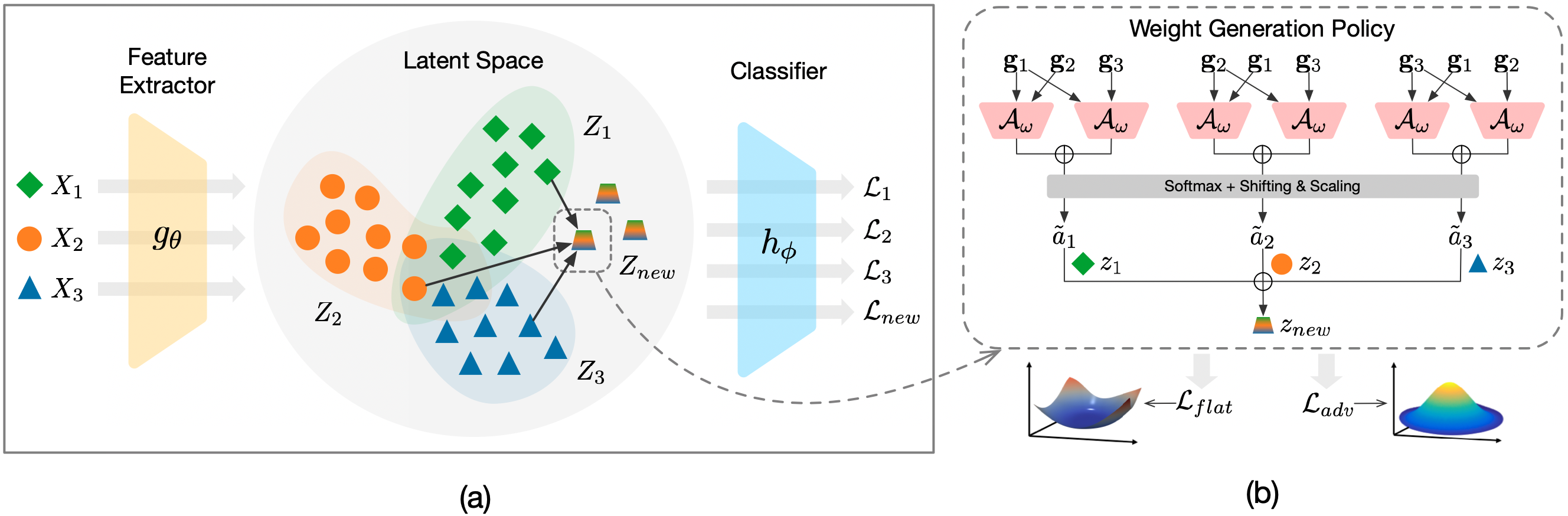
Figure 2: Overview of the proposed FGMix. (a) Latent Code Augmentation: the mixup latent codes $Z_{new}$ are used together with the original latent codes $\{Z_{1},Z_{2},Z_{3}\}$ to train the classifier $h_{\phi}$. (b) Weight Generation Policy: the weight assigned to each latent code is based on the sum of its gradient’s similarities w.r.t. other latent codes. A softmax and a shifting & scaling layers are applied to enable extrapolation. The similarity function $\mathcal{A}_{\omega}$ is learned towards flatter minima (i.e., $\mathcal{L}_{flat}$) and matching the generated codes to a prior via adversarial training (i.e., $\mathcal{L}_{adv}$).

3.2 Gradient-based Weight Generation

Unlike the previous methods which sample weights $\{a_{i}\}_{i=1}^{k}$ from a pre-defined distribution [46, 42, 49, 43], here we consider a context-aware approach which assigns weight to an instance based on its relations with other instances in the same combination. While the feature-based approach specifies similarity in the latent space, it does not indicate what the classifier considers as similar. In order to promote invariant-learning of the classifier, we propose to measure similarity between instances using gradients.

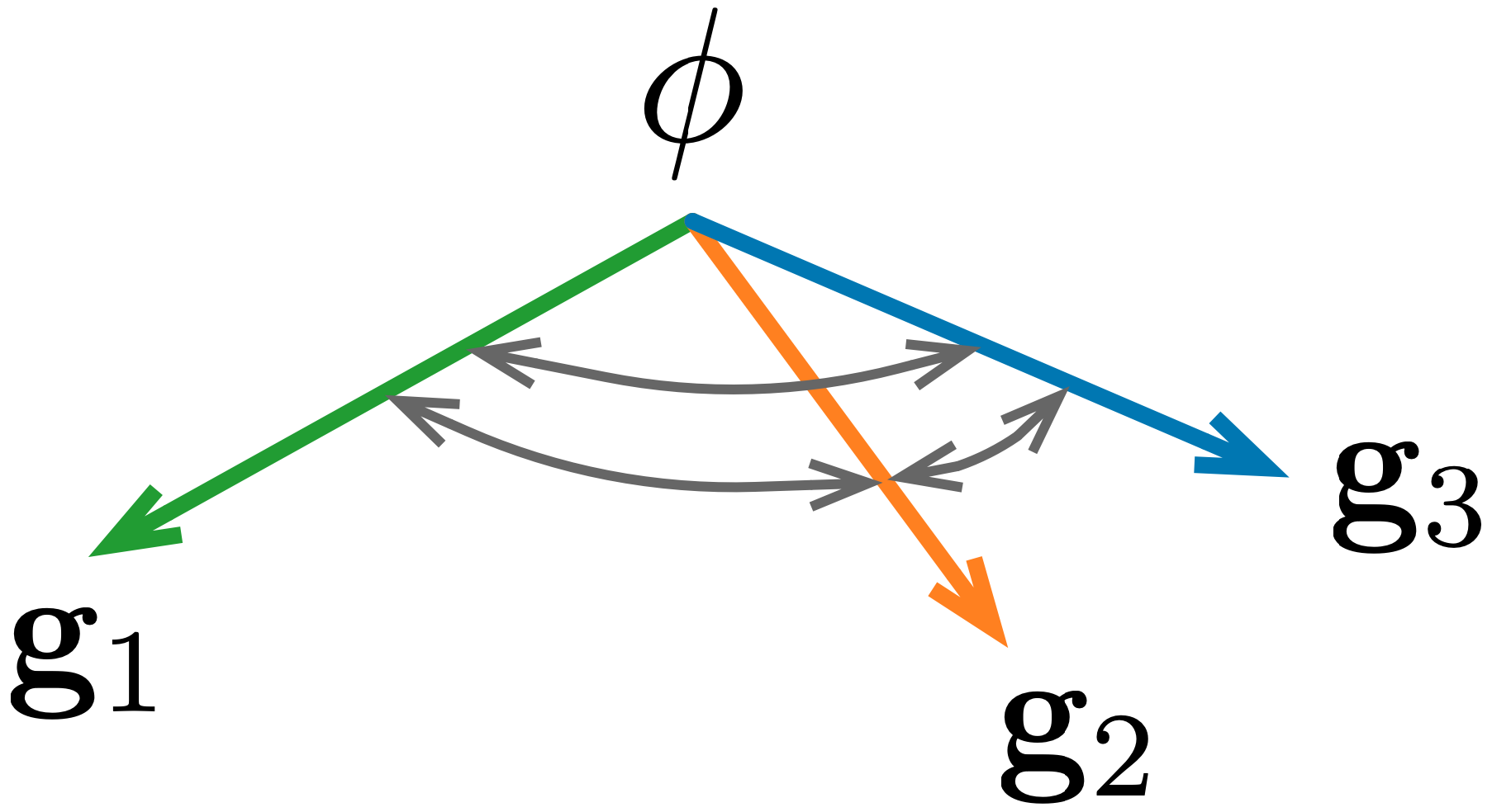
Figure 3: Gradients w.r.t. the classifier $\phi$ for 3 instances.

Gradient similarity indicates the level of information sharing between instances in terms of model learning. To illustrate this, let $\mathbf{g}_{i}$ denote the gradient of the $i$-th instance loss $l(y_{i},h_{\phi}(\mathbf{z}_{i}))$ w.r.t. the classifier $\phi$, i.e., $\mathbf{g}_{i}=\frac{\partial{l(y_{i},h_{\phi}(\mathbf{z}_{i}))}}{\partial{\phi}}$. We consider 3 gradients $\{\mathbf{g}_{1},\mathbf{g}_{2},\mathbf{g}_{3}\}$ of instances $\{\mathbf{z}_{1},\mathbf{z}_{2},\mathbf{z}_{3}\}$ from 3 different domains as shown in Figure 3. Since $\mathbf{g}_{2}$ and $\mathbf{g}_{3}$ are pointing towards similar directions (i.e., $\cos{\psi_{2,3}}>0$, where $\psi_{2,3}$ is the angle between $\mathbf{g}_{2}$ and $\mathbf{g}_{3}$), taking a step along $\mathbf{g}_{2}$ or $\mathbf{g}_{3}$ will improve the classifier’s performance on both $\mathbf{z}_{2}$ and $\mathbf{z}_{3}$. This implies that $\mathbf{z}_{2}$ and $\mathbf{z}_{3}$ contain some shared/invariant information as recognized by the classifier. Conversely, for $\mathbf{g}_{1}$ and $\mathbf{g}_{3}$, since they are pointing towards different directions (i.e., $\cos{\psi_{1,3}}<0$), gradient update on one will degrade the classifier’s performance on the other, as the level of information sharing between $\mathbf{z}_{1}$ and $\mathbf{z}_{3}$ is low. In this specific example, following the direction of $\mathbf{g}_{2}$ seems to be the best option as it helps classify $\mathbf{z}_{3}$ well while will not jeopardize too much the performance on $\mathbf{z}_{1}$. That is, it contains the most invariant information among the 3 candidate instances. This amount of invariant information an instance carries can be quantified by the sum of similarities of the instance’s gradient w.r.t. all the other instances, e.g., $s_{i}=\sum_{j\neq i}\cos{\psi_{i,j}}$, which can be used as a criterion to assign weights.

To endow the weight generation policy with some flexibility to learn towards generating a desired distribution, we employ a learnable similarity function $\mathcal{A}_{\omega}(\cdot,\cdot)$ (instead of a pre-defined similarity function like cosine similarity) to measure the similarity between gradients. Specifically, we compute the sum of gradient similarities $s_{i}$ (also referred to as score) for the $i$-th latent code $\mathbf{z}_{i}$ as:

$$s_{i}=\sum_{j\neq i,j\in\{1,...,k\}}\mathcal{A}_{\omega}(\mathbf{g}_{i},\mathbf{g}_{j}).$$ (3)

In practice, we use a neural network (i.e., 2-layer MLP) to model $\mathcal{A}_{\omega}$, where the two gradients $\mathbf{g}_{i}$ and $\mathbf{g}_{j}$ are concatenated in order (i.e., $\mathbf{g}_{i}$ followed by $\mathbf{g}_{j}$) and fed into the network. Note that this similarity function is asymmetric, i.e., $\mathcal{A}_{\omega}(a,b)\neq\mathcal{A}_{\omega}(b,a)$. Hence, even when we only have 2 source domains, it is possible that the 2 latent codes will be assigned with different weights.

To ensure that the weights sum to 1, we apply a softmax layer on top of the score $s_{i}$:

$$a_{i}=\frac{\exp(s_{i})}{\sum_{i^{\prime}=1}^{k}\exp(s_{i^{\prime}})}.$$ (4)

Since the softmax normalization produces $a_{i}\in(0,1)$, this corresponds to generating $\mathbf{z}_{new}$ as an interpolation of $\{\mathbf{z}_{1},...,\mathbf{z}_{k}\}$. To enable extrapolation, we further introduce a scaling and shifting operation to be applied on $a_{i}$, which lifts off the positivity constraint and allows for weight value to be greater than 1. Generally, it serves to reduce the uncertainty in the weight distribution. Specifically, we introduce a scaling factor $\lambda$ and a shifting factor $\frac{\lambda-1}{k}$ to process the weight $a_{i}$ by:

$$\tilde{a}_{i}=\lambda a_{i}-\frac{\lambda-1}{k},$$ (5)

where the constraint $\sum_{i=1}^{k}\tilde{a}_{i}=1$ is still fulfilled after the processing. The generated $\mathbf{z}_{new}$ is now computed by $\mathbf{z}_{new}=\sum_{i=1}^{k}\tilde{a}_{i}\mathbf{z}_{i}$. Note that for the mixup loss $l_{new}$ in (1), we do not apply the scaling and shifting process on the weights as negative loss values are prohibited. Figure 2(b) depicts the proposed weight generation policy.

3.3 Learning the Weight Generation Policy

As mentioned before, a learnable function $\mathcal{A}_{\omega}$ is employed to compute the similarity between gradients and to generate the instance weights. To encourage better generalization ability of the classifier learned with the augmented latent codes, we propose to optimize $\omega$ towards generating a flatter loss surface in the neighbourhoods of the classifier $\phi$. Generally, the flatness can be measured using Hessian-based quantities [20, 8, 33] or Monte-Carlo approximations of the loss value in the model’s neighbourhoods [11, 6]. For computational efficiency, we adopt the Monte-Carlo approach and measure flatness by the loss difference between the current classifier $\phi$ and its neighbourhoods $\phi^{\prime}$ within $\gamma$ distance. Formally, we optimize $\omega$ with the objective:

$$\mathop{\min}_{\omega}\mathbb{E}_{\|\phi-\phi^{\prime}\|\leq\gamma}[\triangle\mathcal{L}_{new}^{2}],$$ (6)

where $\triangle\mathcal{L}_{new}=\frac{1}{n}\sum_{j=1}^{n}l(y_{new,j},h_{\phi}(\mathbf{z}_{new,j}))-l(y_{new,j},h_{\phi^{\prime}}(\mathbf{z}_{new,j}))$. In practice, we approximate the expectation by sampling 100 directions from a unit sphere.

To prevent the undesirable effects of over-extrapolation, we further impose an auxiliary adversarial loss to constrain that the generated latent codes conform to a prior distribution. Similar to Li et al. [24], we match the generated distribution to a prior via adversarial training. Specifically, a discriminator $d(\cdot)$ is introduced to distinguish the generated latent codes from the ones sampled from the prior distribution. Our weight generation policy will learn to fool the discriminator to believe that the generated codes are from the prior. The minimax objective is formulated as:

$$\mathop{\min}_{\omega}\mathop{\max}_{d}\mathbb{E}_{\hat{\mathbf{z}}_{new}\sim p(\hat{\mathbf{z}}_{new})}[\log d(\hat{\mathbf{z}}_{new})]+\mathbb{E}_{(\mathbf{z}_{1},...,\mathbf{z}_{k})\sim p_{source}(\mathbf{z})}[\log(1-d(\sum_{i=1}^{k}\tilde{a}_{i}\mathbf{z}_{i}))],$$ (7)

where $p(\hat{\mathbf{z}}_{new})$ is a pre-defined prior distribution. In theory, we can use any arbitrary distribution for the prior. Here, we employ a Gaussian whose mean $\mu$ and variance $\sigma^{2}$ are computed from the source domains, i.e., $\mu=\frac{1}{|S|}\sum_{i=1}^{|S|}\mathbf{z}_{i}$ and $\sigma^{2}=\frac{1}{|S|}\sum_{i=1}^{|S|}(\mathbf{z}_{i}-\mu)\circ(\mathbf{z}_{i}-\mu)$, where $\circ$ denotes the Hadamard product (i.e., only the diagonal entries of the covariance matrix are used). In practice, since the feature extractor (and hence the latent distribution) evolves over the course of training, we compute moving averages of the mean and variance of the mini-batch to approximate the Gaussian.

The weight generation policy $\omega$ is jointly learned with the base model $f$, i.e., we optimize (6) and (7) simultaneously with (2). To ensure that the feature extractor is well-trained and produces meaningful latent codes for mixup, learning of ${\omega}$ (as well as the addition of generated latent codes for classifier training) will only commence at the later stage of training (i.e., starting from the $\tau$-th iteration). The overall training procedure is summarized in Algorithm 1.

Required: Source data $S=\{S_{1},...,S_{k}\}$; Total number of iterations $T$; Iteration to start training and applying the weight generation policy $\tau$; Number of mixup instances generated in each iteration $n$; Learning rate of base model $\alpha$; Learning rate of weight generation policy $\beta$; Scaling factor $\lambda$; Neighbourhood size $\gamma$.

Output: Learned feature extractor $g_{\theta}(\cdot)$ and classifier $h_{\phi}(\cdot)$.

1 Randomly initialize all learnable parameters.

2 for $t\in\{1,...,T\}$ do

3       Sample a mini-batch $B=\{B_{1},...,B_{k}\}$ from $k$ source datasets $\{S_{1},...,S_{k}\}$.

4       if $t\geq\tau$ then

5             for $j\in{1,...,n}$ do

6                  Sample $(\mathbf{x}_{i},y_{i})\in B_{i}$ for $i=1,...,k$.

7                   Obtain latent code $\mathbf{z}_{i}=g_{\theta}(\mathbf{x}_{i})$ for $i=1,...,k$.

8                   Compute linear weights $\{\tilde{a}_{i}\}_{i=1}^{k}$ by (3)-(5).

9                   Compute $\mathbf{z}_{new,j}$ and its loss $l_{new,j}$ by (1).

10            Compute weight generation policy loss $\mathcal{L}_{\omega}=\mathbb{E}_{\|\phi-\phi^{\prime}\|\leq\gamma}[\triangle\mathcal{L}_{new}^{2}]+\frac{1}{n}\sum_{j=1}^{n}\log(1-d(\mathbf{z}_{new,j}))$.

11             Compute discriminator loss $\mathcal{L}_{d}=-\frac{1}{n}\sum_{j=1}^{n}(\log d(\hat{\mathbf{z}}_{new,j})+\log(1-d(\mathbf{z}_{new,j})))$.

12             Update policy and discriminator $\omega\leftarrow\omega-\beta\nabla_{\omega}\mathcal{L}_{\omega}$, $d\leftarrow d-\beta\nabla_{d}\mathcal{L}_{d}$.

13             Compute base model loss $\mathcal{L}_{base}=\frac{1}{|B|+n}\left(\sum_{i=1}^{k}\sum_{j=1}^{|B_{i}|}l(y_{i,j},h_{\phi}(g_{\theta}(\mathbf{x}_{i,j})))+\sum_{j=1}^{n}l_{new,j}\right)$.

14            

15      else

16            Compute base model loss $\mathcal{L}_{base}=\frac{1}{|B|}\sum_{i=1}^{k}\sum_{j=1}^{|B_{i}|}l(y_{i,j},h_{\phi}(g_{\theta}(\mathbf{x}_{i,j})))$.

17      Update base model $\theta\leftarrow\theta-\alpha\nabla_{\theta}\mathcal{L}_{base}$, $\phi\leftarrow\phi-\alpha\nabla_{\phi}\mathcal{L}_{base}$.

Algorithm 1 Training Procedure of FGMix

4 Experiments

Dataset Details

We conduct experiments mainly on DomainBed [13], a recently introduced testbed that provides a unified evaluation procedure for DG algorithms. Following the previous DG studies [1, 6], we focus on five real-world benchmark datasets available on DomainBed: PACS [22] (4 domains, 7 classes, and 9,991 images), VLCS [10] (4 domains, 5 classes, and 10,729 images), OfficeHome [41] (4 domains, 65 classes, and 15,588 images), TerraIncognita [3] (4 domains, 10 classes, and 24,788 images) and DomainNet [32] (6 domains, 345 classes, and 586,575 images).

Implementation Details

For a fair comparison, we follow the experimental settings by Gulrajani and Lopez-Paz [13], including data splits (20% data are reserved for validation for each training domain), hyper-parameter search (a search distribution is pre-defined for each hyper-parameter), number of iterations (default to be 5,000), image augmentation (cropping, resizing, horizontal flips, color jitter, grayscaling, normalization, etc.) and the base model backbone (ResNet-50 [16] pre-trained on ImageNet as initialization). For our proposed FGMix, we set the iteration $\tau$ to start training and applying weight generation as 3,000, and the learning rate of weight generation policy $\beta$ as 1e-3. We perform model selection by tuning the scaling factor $\lambda$ from $\text{RandomChoice}([1,3,5,10,20])$ and the neighbourhood size $\gamma$ from $10^{\text{Uniform}(0,2)}$ on the training domain validation sets. All experiments are repeated for 5 trials with different random seeds.

Table 1: Overall comparison of selected algorithms on five datasets. Model selection is based on training domain validation. The result reported for each dataset is the average performance over all the test domains for that dataset. Most of the results are obtained directly from the literature, except for those denoted with ^†, which are from our reproduction on DomainBed.

	Algorithm	PACS	VLCS	OfficeHome	TerraInc	DomainNet	Avg.
	ERM [40]	85.5$\pm$0.2	77.5$\pm$0.4	66.5$\pm$0.3	46.1$\pm$1.8	40.9$\pm$0.1	63.3
Mixup-based Methods	Mixup [43]	84.6$\pm$0.6	77.4$\pm$0.6	68.1$\pm$0.3	47.9$\pm$0.8	39.2$\pm$0.1	63.4
	Manifold Mixup† [42]	86.2$\pm$0.6	76.7$\pm$1.1	67.3$\pm$1.0	48.8$\pm$2.1	41.2$\pm$0.3	64.0
	MixStyle† [49]	85.3$\pm$1.9	77.4$\pm$0.8	67.3$\pm$0.9	46.8$\pm$1.1	40.9$\pm$0.2	63.5
	MetaMixup† [27]	85.2$\pm$1.2	77.9$\pm$0.8	68.2$\pm$0.7	47.1$\pm$1.8	41.8$\pm$0.3	64.0
Gradient-based Methods	PCGrad† [44]	85.0$\pm$0.9	77.5$\pm$0.8	65.5$\pm$0.9	48.3$\pm$2.3	41.1$\pm$0.2	63.5
	AND-Mask [31]	84.4$\pm$0.9	78.1$\pm$0.9	65.6$\pm$0.4	44.6$\pm$0.3	37.2$\pm$0.6	62.0
	Fish [37]	85.5$\pm$0.3	77.8$\pm$0.3	68.6$\pm$0.4	45.1$\pm$1.3	42.7$\pm$0.2	63.9
	Fishr [34]	85.5$\pm$0.4	77.8$\pm$0.1	67.8$\pm$0.1	47.4$\pm$1.6	41.7$\pm$0.0	64.0
Augmentation Methods	L2A-OT† [48]	85.8$\pm$1.9	77.4$\pm$0.9	68.1$\pm$1.6	48.6$\pm$2.1	40.2$\pm$0.5	64.0
	CNSN† [39]	85.6$\pm$0.9	77.1$\pm$1.0	67.3$\pm$1.2	48.4$\pm$1.6	40.7$\pm$0.4	63.8
	DDG† [47]	85.3$\pm$1.6	76.8$\pm$1.2	68.1$\pm$1.0	47.7$\pm$2.1	40.0$\pm$0.5	63.6
DomainBed SOTA	SelfReg [21]	85.6$\pm$0.4	77.8$\pm$0.9	67.9$\pm$0.7	47.0$\pm$0.3	41.5$\pm$0.2	64.0
	SagNet [30]	86.3$\pm$0.2	77.8$\pm$0.5	68.1$\pm$0.1	48.6$\pm$1.0	40.3$\pm$0.1	64.2
	CORAL [38]	86.2$\pm$0.3	78.8$\pm$0.6	68.7$\pm$0.3	47.6$\pm$1.0	41.5$\pm$0.1	64.6
	FGMix (ours)	86.6$\pm$1.1	77.9$\pm$0.7	68.9$\pm$1.2	49.0$\pm$1.6	42.0$\pm$0.4	64.9
Combined with flatness-aware solver SWA [18, 1]
	ERM + SWA†	87.0$\pm$0.5	77.2$\pm$0.6	69.5$\pm$0.4	50.1$\pm$0.7	44.0$\pm$0.2	65.6
	SelfReg + SWA	86.5$\pm$0.3	77.5$\pm$0.0	69.4$\pm$0.2	51.0$\pm$0.4	44.6$\pm$0.1	65.8
	CORAL + SWA†	87.5$\pm$0.5	78.2$\pm$0.4	70.7$\pm$0.1	51.1$\pm$0.6	44.6$\pm$0.4	66.4
	FGMix + SWA (ours)	88.5$\pm$0.7	78.8$\pm$0.6	71.4$\pm$0.3	52.2$\pm$0.9	45.1$\pm$0.3	67.2

Table 2: Ablation study on PACS and TerraInc. From A to FGMix we add one component at a time, where A is simply interpolation with random weights. We test for both w/o and w/ SWA.

Variant	Components					w/o SWA		w/ SWA
	similarity- based weights	gradient- based similarity	scaling & shifting	$\mathcal{L}_{flat}$	$\mathcal{L}_{adv}$	PACS	TerraInc	PACS	TerraInc	Avg.
A (baseline)						84.3$\pm$0.8	48.1$\pm$0.9	86.7$\pm$0.8	50.2$\pm$0.8	67.4
B	✓					85.4$\pm$0.7	48.0$\pm$0.7	87.4$\pm$0.5	50.9$\pm$1.2	67.9
C	✓	✓				85.5$\pm$0.2	48.0$\pm$1.4	87.9$\pm$0.3	51.4$\pm$0.7	68.2
D	✓	✓	✓			85.8$\pm$0.9	48.8$\pm$1.5	87.7$\pm$0.9	51.5$\pm$1.1	68.5
E	✓	✓	✓	✓		86.5$\pm$1.6	49.1$\pm$2.1	88.2$\pm$1.2	52.0$\pm$1.5	69.0
FGMix (ours)	✓	✓	✓	✓	✓	86.6$\pm$1.1	49.0$\pm$1.6	88.5$\pm$0.7	52.2$\pm$0.9	69.1

4.1 Overall Comparison

We select several baselines related to our method for overall comparison on DomainBed: (1) naive baseline without any DG strategy: ERM [40] (empirical risk minimization); (2) mixup-based methods: Mixup [43] (mixup at the input level), Manifold Mixup [42] (mixup at the feature level), MixStyle [49] (mixup of feature statistics) and MetaMixup [27] (meta-learn the interpolation policy); (3) gradient-based methods: PCGrad [44] (project gradients onto the normal plane of conflicting gradients), AND-Mask [31] (mask out conflicting gradient components), Fish [37] (gradient alignment) and Fishr [34] (gradient covariance alignment); (4) augmentation methods: L2A-OT [48] (generate pseudo-source by enlarging divergence to the source domains), CNSN [39] (exchange and normalize instances’ styles), DDG [47] (disentangle and swap instances’ variation factors) (5) current SOTA on DomainBed: SagNet [30] (reduce style bias), SelfReg [21] (self-supervised contrastive regularization) and CORAL [38] (correlation alignment). Hyper-parameters settings of the baselines reproduced by us can be found in Appendix B.

The results on 5 datasets are presented in Table 1 (see Appendix A.1 for results on each test domain). We observe that most of the DG algorithms outperform ERM in terms of average accuracy (except for AND-Mask). Our proposed FGMix achieves consistent performance gains over ERM for all the 5 datasets: +1.1pp for PACS, +0.4pp for VLCS, +2.4pp for OfficeHome, +2.9pp for TerraInc and +1.1pp for DomainNet. We notice that FGMix performs exceptionally well on the more challenging datasets where the distribution shifts between source and target domains might be significant, i.e., the gains are most significant for OfficeHome and TerraInc whose test accuracies are relatively low as compared to other datasets. Overall, our FGMix tops in 3 out of 5 datasets, achieving the best average accuracy with 0.3pp higher than the previous SOTA (CORAL), and 0.9pp higher than the strongest related baselines (Manifold Mixup, MetaMixup, Fishr and L2A-OT).

We further conduct experiments to combine FGMix with the flatness-aware solver SWA (Stochastic Weight Averaging) [18, 1]. SWA simply performs weight averaging which yields minimizer at the flatter central region of the minimum. A recent study by Arpit et al. [1] found that SWA not only boosts performance of DG algorithms, but also ensures better correlation between in-domain validation and out-domain test results, facilitating more reliable model selection. We combine SWA with FGMix and 3 other strong and representative DG algorithms (i.e., ERM, SelfReg and CORAL) for comparison. From Table 1, we see that FGMix + SWA achieves the best results for all 5 datasets. Notably, the average gain of FGMix over CORAL increases from 0.3pp to 0.8pp after combining with SWA. This shows that FGMix is more orthogonal to SWA, as its benefits still persist after combining with SWA. To understand the reason behind, recall that FGMix serves to widen the loss surface for the optimizer to explore. While this increases the chance of covering the target area, it also enlarges the reachable off-target area. SWA with weight averaging along the training helps mitigate the risk of optimizer running into undesirable region.

4.2 Ablation Study

We test the efficacy of various components of FGMix by introducing 5 variants, each includes one more component at a time: A is a simple interpolation baseline with random instance weights drawn from Dirichlet distribution; B employs cosine similarity to compute the weights based on instances’ feature vectors; C computes similarity based on instances’ gradients w.r.t. the classifier; D further includes the scaling & shifting process to enable extrapolation; E replaces the cosine similarity with a learnable similarity function and optimizes it towards the flatness-aware loss $\mathcal{L}_{flat}$. Further including the adversarial training for prior matching results in our proposed FGMix.

Table 2 presents the results (see Appendix A.2 for results on each test domain). Based on the average results, from A to FGMix we obtain the incremental gains: +0.5pp, +0.3pp, +0.3pp, +0.5pp, +0.1pp. Firstly, similarity-based weights with attention to the other instances involved in the same combination give better performance than the random weights. Replacing feature-based similarity with gradient-based similarity further improves the performance, as gradients indicate what the classifier considers as invariant information. Enabling data extrapolation (i.e., scaling & shifting) and learning towards flatter loss surface (i.e., $\mathcal{L}_{flat}$) both serve to increase the chance of covering the target domain. Last but not least, though matching the generated distribution to a prior (i.e., $\mathcal{L}_{adv}$) may seem to have minor effects on the mean accuracies, it helps reduce the variance significantly from E to FGMix, demonstrating its regularization effects to prevent over-extrapolation.

4.3 Qualitative Analysis

4.3.1 Mixup Distribution Visualization

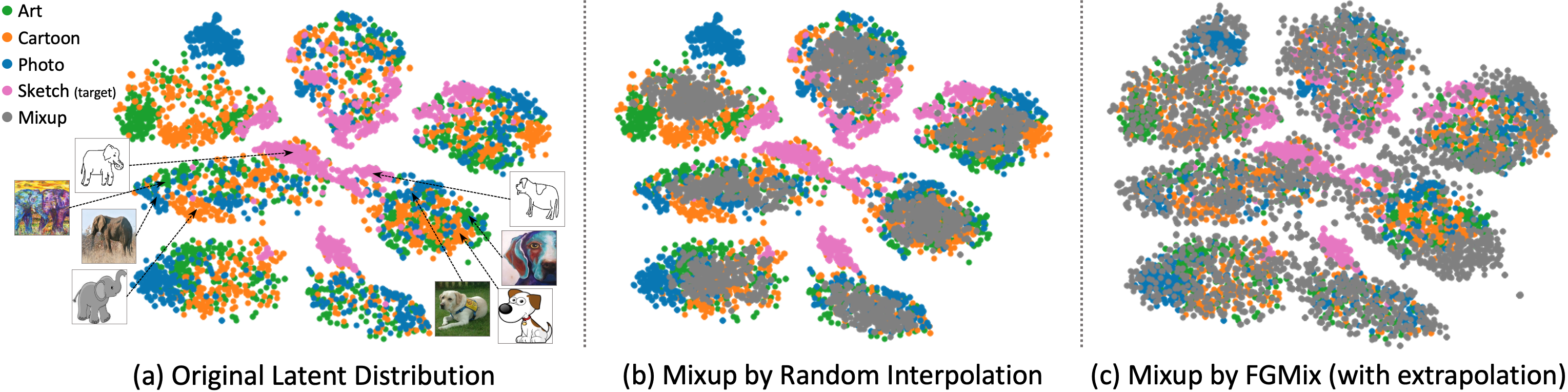
Figure 4: t-SNE visualization of the latent distributions of PACS trained by using “Art", “Cartoon", “Photo" as the source domains and “Sketch" as the target domain. We plot the mixup distribution generated by random interpolation and by our FGMix which involves extrapolation. For clearer visualization, the mixup is generated using same-class examples.

To understand how the generated distribution facilitates the learning of classifier, we visualize the latent codes of PACS in 2D space using t-SNE. For this visualization, we train a model (i.e., feature extractor + classifier) with FGMix and obtain the latent codes from the feature extractor. To compare different mixup methods, we plot the mixup distribution generated by random interpolation (i.e., variant A) and by our FGMix which involves extrapolation. For clearer visualization, the mixup is generated using same-class examples. In this experiment, we use “Sketch" as the target domain, as it is the most difficult domain when training with the other 3 domains.

Figure 4 shows the distributions of the original latent codes (4a) and the mixup latent codes generated by random interpolation (4b) and by FGMix (4c) respectively. Firstly, we see that by training with FGMix, 7 clusters corresponding to 7 class labels are clearly separated in the learned latent space. In 4a, we observe that the latent codes of the target domain “Sketch" (i.e., the pink dots) are located near the decision boundary, especially for the “dog" and “elephant" categories which are inseparable at the central region. In 4b, the mixup codes generated by random interpolation mostly lie within the convex hull formed by the source latent codes in the respective cluster, leaving the target region uncovered. Our FGMix with extrapolation, on the other hand, is able to generate codes outside of the convex hull (as shown in 4c), resulting in better coverage of the target region and hence better generalization of the classifier learned from the mixup latent codes.

4.3.2 Loss Landscape Visualization

In this section, we verify that FGMix indeed generates a flatter loss surface. We also observe how the change in loss landscape affects the optimization process. The experiments are conducted on TerraInc dataset using “L100", “L43", “L45" as the source domains and “L38" as the target domain. Additional visualization on other target domains can be found in Appendix A.3.

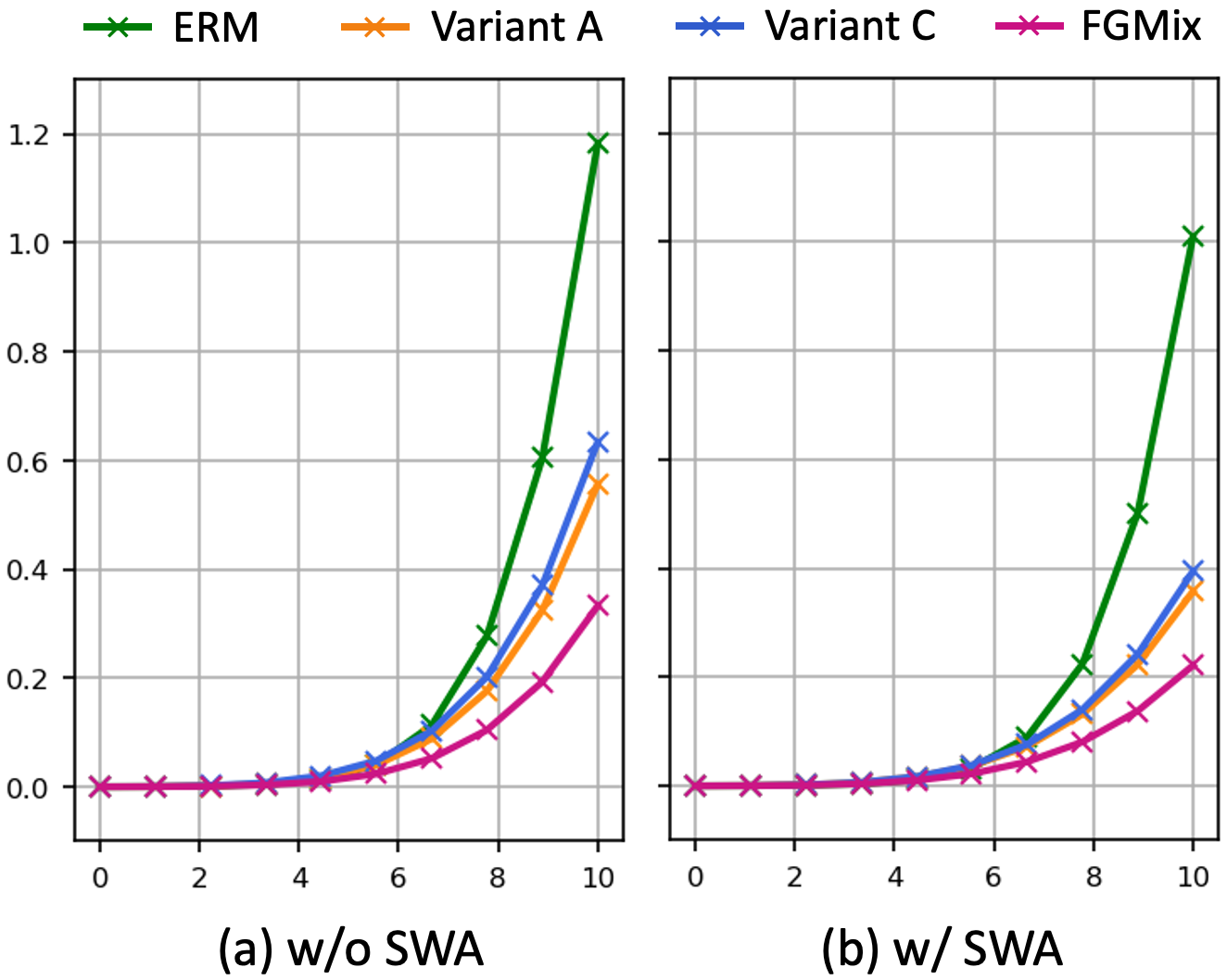
Figure 5: We plot for 4 methods the square loss difference between the minimizer and its neighbourhoods at distance $\gamma=1,...,10$. The value is averaged over 50 random directions.

Flatness Analysis

We compare the flatness of FGMix minimizer with that of ERM, random mixup (i.e., variant A) and gradient-based similarity mixup (i.e., variant C), for both w/o and w/ SWA. Following Izmailov et al. [18], Cha et al. [6], for each method, we plot the square loss difference between the minimizer $\phi^{*}$ and its neighbourhoods $\phi^{\prime}$ at distance $\gamma$, i.e., $\mathbb{E}_{\|\phi^{*}-\phi^{\prime}\|=\gamma}[\mathcal{L}(\phi^{*})-\mathcal{L}(\phi^{\prime})]^{2}$, for $\gamma=1,...,10$. The expectation is approximated by averaging over 50 randomly sampled directions. Note that for ERM, the loss is based on the original training data, while for variant A, variant C and FGMix, the loss is based on the mixture of original and mixup data. Figure 5 shows the plots for w/o and w/ SWA. We see that applying SWA results in flatter minima for all methods. Comparing ERM with variant A and C, we see that simply adding mixup data yields flatter loss surface. Our FGMix explicitly optimized for smaller loss difference further flattens the minima compared to its variants.

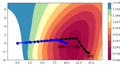
(a) ERM Train Loss Surface

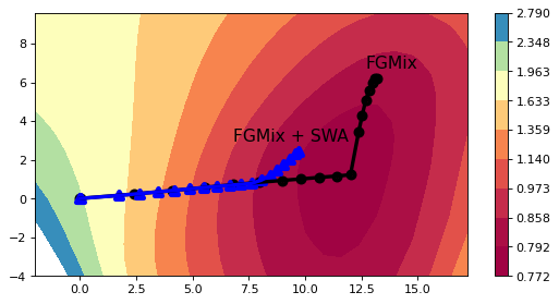
(b) FGMix Train Loss Surface

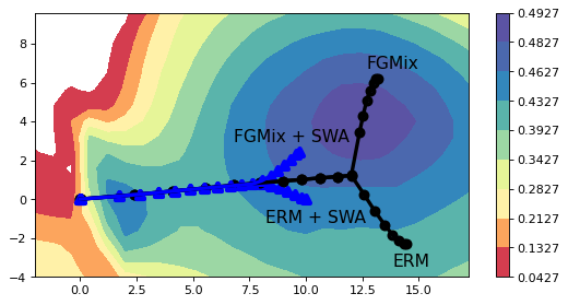
(c) Test Accuracy Surface

Figure 6: 2D loss and accuracy surfaces generated using 3 models at the initialization, the end of ERM + SWA, and the end of FGMix + SWA respectively. Note that only these 3 models are actually on the 2D plane. Also note that since (b) is the loss surface including the mixup data, while the mixup data is only added for FGMix training from the 3,000-th iteration onwards, the loss values indicated for the optimization path before the 3,000-th iteration in (b) do not reflect the actual loss during training. For direct comparison of the flatness, we use the same scale interval for (a) and (b).

Loss Surface & Optimization Path

To observe how the generated data affects the optimization, we plot the 2D loss surface of the original training data (i.e., ERM) as well as the one after adding the generated data (i.e., FGMix). We also plot the accuracy surface of the test data to visualize the distribution shifts from the training domains. Note that we include the generated data for model training only from the 3,000-th iteration onwards, hence ERM and FGMix will have the exact same path for the first 2,999 steps, and start to diverge from the 3,000-th step. We consider the original optimization paths of ERM and FGMix and the ones with SWA, as weight averaging helps stablize the optimization paths and converge to better minima. To generate the 2D loss surface, we follow Izmailov et al. [18] by choosing 3 models to compute the orthonormal basis of the 2D plane (more details included in Appendix A.4). For better span of the 2D perspective, the 3 models selected are 1) at the initialization, 2) at the end of ERM + SWA, and 3) at the end of FGMix + SWA.

Figure 6 shows the train loss surfaces of ERM and FGMix and the respective optimization paths (14(a) & 14(b)), and the test accuracy surface with both paths on it (14(c)). Firstly, we observe that the loss surface of FGMix is wider and flatter. Comparing the loss surface of ERM with the test accuracy surface, we see that there is a clear shift in optimum. With wider minimum in the FGMix loss surface, the test maximum is better covered, and the optimization converges to a point with higher test accuracy (i.e., in 14(c), FGMix + SWA terminates at a darker region than ERM + SWA).

5 Conclusion and Discussion

In this work, we explore a mixup method with data extrapolation. We propose a weight generation policy named FGMix, which computes instance weights based on gradients and learns towards flatter minima. We also employ an adversarial loss for regularization. Extensive experiments on the DomainBed benchmark demonstrates FGMix’s effectiveness. Perhaps the major limitation of FGMix is the large variance caused by data extrapolation, as we lack strategies to direct the extrapolation towards the expected region. In the future, we will consider exploiting the domain-specific information as well as the source domain relations to design a more effective extrapolation strategy.

Appendix A Additional Experimental Results

A.1 Full Results for Overall Comparison

Table 3: Overall comparison of selected algorithms on PACS.

	Algorithm	A	C	P	S	Avg.
	ERM [40]	84.7$\pm$0.4	80.8$\pm$0.6	97.2$\pm$0.3	79.3$\pm$1.0	85.5
Mixup-based Methods	Mixup [43]	86.1$\pm$0.5	78.9$\pm$0.8	97.6$\pm$0.1	75.8$\pm$1.8	84.6
	Manifold Mixup† [42]	88.8$\pm$0.6	80.9$\pm$0.9	95.8$\pm$0.7	79.8$\pm$0.1	86.2
	MixStyle† [49]	83.7$\pm$0.1	80.7$\pm$3.7	95.5$\pm$1.2	81.4$\pm$2.6	85.3
	MetaMixup† [27]	84.9$\pm$1.5	79.6$\pm$0.6	96.3$\pm$0.9	80.1$\pm$1.4	85.2
Gradient-based Methods	PCGrad† [44]	85.9$\pm$1.0	80.4$\pm$0.1	95.5$\pm$0.1	78.2$\pm$2.2	85.0
	AND-Mask [31]	85.3$\pm$1.4	79.2$\pm$2.0	96.9$\pm$0.4	76.2$\pm$1.4	84.4
	Fish [37]	-	-	-	-	85.5
	Fishr [34]	88.4$\pm$0.2	78.7$\pm$0.7	97.0$\pm$0.1	77.8$\pm$2.0	85.5
Augmentation Methods	L2A-OT† [48]	87.9$\pm$1.5	81.4$\pm$2.3	96.7$\pm$1.3	77.2$\pm$2.4	85.8
	CNSN† [39]	86.7$\pm$0.2	80.2$\pm$1.1	96.2$\pm$0.7	79.2$\pm$1.5	85.6
	DDG† [47]	87.4$\pm$1.2	79.2$\pm$1.8	97.4$\pm$1.2	77.3$\pm$2.1	85.3
DomainBed SOTA	SelfReg [21]	87.9$\pm$1.0	79.4$\pm$1.4	96.8$\pm$0.7	78.3$\pm$1.2	85.6
	SagNet [30]	87.4$\pm$1.0	80.7$\pm$0.6	97.1$\pm$0.1	80.0$\pm$0.4	86.3
	CORAL [38]	88.3$\pm$0.2	80.0$\pm$0.5	97.5$\pm$0.3	78.8$\pm$1.3	86.2
	FGMix (ours)	87.2$\pm$1.0	81.2$\pm$1.0	97.9$\pm$0.8	80.2$\pm$1.4	86.6
Combined with flatness-aware solver SWA [18, 1]
	ERM + SWA†	88.1$\pm$0.6	82.0$\pm$0.6	96.9$\pm$0.5	80.8$\pm$0.2	87.0
	SelfReg + SWA	85.9$\pm$0.6	81.9$\pm$0.4	96.8$\pm$0.1	81.4$\pm$0.6	86.5
	CORAL + SWA†	87.6$\pm$0.3	83.1$\pm$0.7	97.5$\pm$0.2	81.6$\pm$0.8	87.5
	FGMix + SWA (ours)	90.4$\pm$0.9	83.0$\pm$0.7	97.8$\pm$0.4	82.8$\pm$0.6	88.5

Table 4: Overall comparison of selected algorithms on VLCS.

	Algorithm	C	L	S	V	Avg.
	ERM [40]	97.7$\pm$0.4	64.3$\pm$0.9	73.4$\pm$0.5	74.6$\pm$1.3	77.5
Mixup-based Methods	Mixup [43]	98.3$\pm$0.6	64.8$\pm$1.0	72.1$\pm$0.5	74.3$\pm$0.8	77.4
	Manifold Mixup† [42]	97.4$\pm$1.3	63.8$\pm$1.9	73.7$\pm$0.0	72.0$\pm$1.3	76.7
	MixStyle† [49]	97.9$\pm$0.7	63.3$\pm$1.7	70.7$\pm$0.2	77.5$\pm$0.4	77.4
	MetaMixup† [27]	98.6$\pm$1.2	63.4$\pm$0.8	72.8$\pm$0.1	76.7$\pm$1.1	77.9
Gradient-based Methods	PCGrad† [44]	98.1$\pm$0.1	66.2$\pm$0.1	70.1$\pm$1.1	75.7$\pm$1.9	77.5
	AND-Mask [31]	97.8$\pm$0.4	64.3$\pm$1.2	73.5$\pm$0.7	76.8$\pm$2.6	78.1
	Fish [37]	-	-	-	-	77.8
	Fishr [34]	98.9$\pm$0.3	64.0$\pm$0.5	71.5$\pm$0.2	76.8$\pm$0.7	77.8
Augmentation Methods	L2A-OT† [48]	98.2$\pm$0.8	64.1$\pm$0.4	71.6$\pm$1.5	75.5$\pm$0.8	77.4
	CNSN† [39]	97.9$\pm$0.4	65.2$\pm$1.3	69.8$\pm$1.4	75.6$\pm$0.7	77.1
	DDG† [47]	98.5$\pm$0.9	64.2$\pm$1.7	70.2$\pm$0.8	74.3$\pm$1.4	76.8
DomainBed SOTA	SelfReg [21]	96.7$\pm$0.4	65.2$\pm$1.2	73.1$\pm$1.3	76.2$\pm$0.7	77.8
	SagNet [30]	97.9$\pm$0.4	64.5$\pm$0.5	71.4$\pm$1.3	77.5$\pm$0.5	77.8
	CORAL [38]	98.3$\pm$0.1	66.1$\pm$1.2	73.4$\pm$0.3	77.5$\pm$1.2	78.8
	FGMix (ours)	97.4$\pm$0.6	64.3$\pm$1.1	72.7$\pm$0.8	77.3$\pm$0.5	77.9
Combined with flatness-aware solver SWA [18, 1]
	ERM + SWA†	97.0$\pm$0.9	64.3$\pm$0.8	72.4$\pm$0.6	75.2$\pm$0.1	77.2
	SelfReg + SWA	97.4$\pm$0.4	63.5$\pm$0.3	72.6$\pm$0.1	76.7$\pm$0.7	77.5
	CORAL + SWA†	98.6$\pm$0.3	63.2$\pm$0.2	72.8$\pm$0.2	78.2$\pm$1.1	78.2
	FGMix + SWA (ours)	98.2$\pm$0.6	63.3$\pm$0.1	75.1$\pm$0.4	78.6$\pm$1.6	78.8

Table 5: Overall comparison of selected algorithms on OfficeHome.

	Algorithm	A	C	P	R	Avg.
	ERM [40]	61.3$\pm$0.7	52.4$\pm$0.3	75.8$\pm$0.1	76.6$\pm$0.3	66.5
Mixup-based Methods	Mixup [43]	62.4$\pm$0.8	54.8$\pm$0.6	76.9$\pm$0.3	78.3$\pm$0.2	68.1
	Manifold Mixup† [42]	61.6$\pm$0.8	55.1$\pm$3.1	75.6$\pm$0.2	77.0$\pm$0.0	67.3
	MixStyle† [49]	61.7$\pm$0.6	53.3$\pm$1.6	76.3$\pm$1.0	77.8$\pm$0.5	67.3
	MetaMixup† [27]	63.5$\pm$1.1	54.6$\pm$0.4	75.9$\pm$0.9	78.7$\pm$0.4	68.2
Gradient-based Methods	PCGrad† [44]	60.6$\pm$1.1	52.1$\pm$1.7	74.4$\pm$0.6	74.0$\pm$0.3	65.5
	AND-Mask [31]	59.5$\pm$1.2	51.7$\pm$0.2	73.9$\pm$0.4	77.1$\pm$0.2	65.6
	Fish [37]	-	-	-	-	68.6
	Fishr [34]	62.4$\pm$0.5	54.4$\pm$0.4	76.2$\pm$0.5	78.3$\pm$0.1	67.8
Augmentation Methods	L2A-OT† [48]	64.5$\pm$1.0	53.8$\pm$2.8	76.2$\pm$1.3	77.9$\pm$1.1	68.1
	CNSN† [39]	63.1$\pm$0.7	53.2$\pm$2.1	74.1$\pm$1.3	78.6$\pm$0.6	67.3
	DDG† [47]	63.7$\pm$0.8	54.5$\pm$1.2	75.9$\pm$1.0	78.2$\pm$0.9	68.1
DomainBed SOTA	SelfReg [21]	63.6$\pm$1.4	53.1$\pm$1.0	76.9$\pm$0.4	78.1$\pm$0.4	67.9
	SagNet [30]	63.4$\pm$0.2	54.8$\pm$0.4	75.8$\pm$0.4	78.3$\pm$0.3	68.1
	CORAL [38]	65.3$\pm$0.4	54.4$\pm$0.5	76.5$\pm$0.1	78.4$\pm$0.5	68.7
	FGMix (ours)	64.2$\pm$1.9	55.3$\pm$1.7	77.1$\pm$0.5	79.1$\pm$0.8	68.9
Combined with flatness-aware solver SWA [18, 1]
	ERM + SWA†	65.7$\pm$1.1	56.2$\pm$0.4	77.3$\pm$0.1	78.9$\pm$0.6	69.5
	SelfReg + SWA	64.9$\pm$0.8	55.4$\pm$0.6	78.4$\pm$0.2	78.8$\pm$0.1	69.4
	CORAL + SWA†	68.3$\pm$0.2	57.0$\pm$0.0	77.9$\pm$0.3	79.7$\pm$0.0	70.7
	FGMix + SWA (ours)	67.9$\pm$0.6	58.1$\pm$0.5	78.9$\pm$0.2	80.6$\pm$0.1	71.4

Table 6: Overall comparison of selected algorithms on TerraIncognita.

	Algorithm	L100	L38	L43	L46	Avg.
	ERM [40]	49.8$\pm$4.4	42.1$\pm$1.4	56.9$\pm$1.8	35.7$\pm$3.9	46.1
Mixup-based Methods	Mixup [43]	59.6$\pm$2.0	42.2$\pm$1.4	55.9$\pm$0.8	33.9$\pm$1.4	47.9
	Manifold Mixup† [42]	57.7$\pm$2.9	42.4$\pm$3.0	55.8$\pm$0.4	39.2$\pm$1.9	48.8
	MixStyle† [49]	53.9$\pm$0.6	42.3$\pm$0.9	53.2$\pm$2.7	37.6$\pm$0.1	46.8
	MetaMixup† [27]	53.2$\pm$1.7	43.7$\pm$2.6	54.5$\pm$1.9	36.9$\pm$1.1	47.1
Gradient-based Methods	PCGrad† [44]	55.9$\pm$2.0	43.2$\pm$3.8	56.4$\pm$2.5	37.7$\pm$1.0	48.3
	AND-Mask [31]	50.0$\pm$2.9	40.2$\pm$0.8	53.3$\pm$0.7	34.8$\pm$1.9	44.6
	Fish [37]	-	-	-	-	45.1
	Fishr [34]	50.2$\pm$3.9	43.9$\pm$0.8	55.7$\pm$2.2	39.8$\pm$1.0	47.4
Augmentation Methods	L2A-OT† [48]	58.7$\pm$2.0	43.5$\pm$2.7	54.8$\pm$1.9	37.4$\pm$1.8	48.6
	CNSN† [39]	58.2$\pm$1.9	43.2$\pm$2.1	57.1$\pm$1.3	35.2$\pm$1.1	48.4
	DDG† [47]	59.6$\pm$3.0	41.2$\pm$2.4	56.0$\pm$1.8	33.9$\pm$1.2	47.7
DomainBed SOTA	SelfReg [21]	48.8$\pm$0.9	41.3$\pm$1.8	57.3$\pm$0.7	40.6$\pm$0.9	47.0
	SagNet [30]	53.0$\pm$2.9	43.0$\pm$2.5	57.9$\pm$0.6	40.4$\pm$1.3	48.6
	CORAL [38]	51.6$\pm$2.4	42.2$\pm$1.0	57.0$\pm$1.0	39.8$\pm$2.9	47.6
	FGMix (ours)	53.7$\pm$3.7	45.0$\pm$0.7	56.9$\pm$0.9	40.6$\pm$1.1	49.0
Combined with flatness-aware solver SWA [18, 1]
	ERM + SWA†	53.5$\pm$0.9	47.6$\pm$0.8	58.2$\pm$0.4	41.0$\pm$0.8	50.1
	SelfReg + SWA	56.8$\pm$0.9	44.7$\pm$0.6	59.6$\pm$0.3	42.9$\pm$0.8	51.0
	CORAL + SWA†	55.6$\pm$0.5	48.1$\pm$0.7	58.5$\pm$0.1	42.2$\pm$1.0	51.1
	FGMix + SWA (ours)	55.7$\pm$1.5	49.4$\pm$1.0	60.6$\pm$0.4	43.2$\pm$0.8	52.2

Table 7: Overall comparison of selected algorithms on DomainNet.

	Algorithm	clip	info	paint	quick	real	sketch	Avg.
	ERM [40]	58.1$\pm$0.3	18.8$\pm$0.3	46.7$\pm$0.3	12.2$\pm$0.4	59.6$\pm$0.1	49.8$\pm$0.4	40.9
Mixup-based Methods	Mixup [43]	55.7$\pm$0.3	18.5$\pm$0.5	44.3$\pm$0.5	12.5$\pm$0.4	55.8$\pm$0.3	48.2$\pm$0.5	39.2
	Manifold Mixup† [42]	60.7$\pm$0.4	19.4$\pm$0.1	47.1$\pm$0.3	11.4$\pm$0.2	59.6$\pm$0.6	48.7$\pm$0.2	41.2
	MixStyle† [49]	59.9$\pm$0.2	19.0$\pm$0.3	47.0$\pm$0.1	11.5$\pm$0.1	58.9$\pm$0.4	48.8$\pm$0.0	40.9
	MetaMixup† [27]	60.7$\pm$0.3	20.0$\pm$0.5	47.1$\pm$0.4	12.8$\pm$0.1	60.1$\pm$0.1	50.1$\pm$0.3	41.8
Gradient-based Methods	PCGrad† [44]	60.3$\pm$0.2	18.1$\pm$0.4	47.0$\pm$0.4	12.9$\pm$0.1	59.8$\pm$0.0	48.4$\pm$0.3	41.1
	AND-Mask [31]	52.3$\pm$0.8	16.6$\pm$0.3	41.6$\pm$1.1	11.3$\pm$0.1	55.8$\pm$0.4	45.4$\pm$0.9	37.2
	Fish [37]	-	-	-	-	-	-	42.7
	Fishr [34]	58.2$\pm$0.5	20.2$\pm$0.2	47.7$\pm$0.3	12.7$\pm$0.2	60.3$\pm$0.2	50.8$\pm$0.1	41.7
Augmentation Methods	L2A-OT† [48]	58.7$\pm$0.3	18.5$\pm$0.4	46.2$\pm$0.5	11.3$\pm$0.7	57.6$\pm$0.8	48.9$\pm$0.2	40.2
	CNSN† [39]	60.2$\pm$0.2	19.0$\pm$0.1	46.3$\pm$0.5	11.6$\pm$0.3	58.2$\pm$0.6	48.7$\pm$0.4	40.7
	DDG† [47]	59.7$\pm$0.5	18.7$\pm$0.2	45.1$\pm$0.9	12.1$\pm$0.4	56.8$\pm$0.3	47.5$\pm$0.7	40.0
DomainBed SOTA	SelfReg [21]	58.5$\pm$0.1	20.7$\pm$0.1	47.3$\pm$0.3	13.1$\pm$0.3	58.2$\pm$0.2	51.1$\pm$0.3	41.5
	SagNet [30]	57.7$\pm$0.3	19.0$\pm$0.2	45.3$\pm$0.3	12.7$\pm$0.5	58.1$\pm$0.5	48.8$\pm$0.2	40.3
	CORAL [38]	59.2$\pm$0.1	19.7$\pm$0.2	46.6$\pm$0.3	13.4$\pm$0.4	59.8$\pm$0.2	50.1$\pm$0.6	41.5
	FGMix (ours)	61.7$\pm$0.2	19.8$\pm$0.6	46.5$\pm$0.4	12.9$\pm$0.1	61.1$\pm$0.4	50.2$\pm$0.9	42.0
Combined with flatness-aware solver SWA [18, 1]
	ERM + SWA†	62.0$\pm$0.1	21.0$\pm$0.0	50.8$\pm$0.2	13.6$\pm$0.3	62.7$\pm$0.1	54.0$\pm$0.2	44.0
	SelfReg + SWA	62.4$\pm$0.1	22.6$\pm$0.1	51.8$\pm$0.1	14.3$\pm$0.1	62.5$\pm$0.2	53.8$\pm$0.3	44.6
	CORAL + SWA†	63.0$\pm$0.3	22.1$\pm$0.5	51.7$\pm$0.4	14.9$\pm$0.5	63.0$\pm$0.3	53.1$\pm$0.1	44.6
	FGMix + SWA (ours)	63.8$\pm$0.3	21.1$\pm$0.6	52.5$\pm$0.2	15.0$\pm$0.1	64.0$\pm$0.2	54.4$\pm$0.2	45.1

A.2 Full Results for Ablation Study

Table 8: Ablation study of FGMix on PACS w/o SWA.

Variant	Components					w/o SWA
	similarity- based weights	gradient- based similarity	scaling & shifting	$\mathcal{L}_{flat}$	$\mathcal{L}_{adv}$	A	C	P	S	Avg.
A (baseline)						85.2$\pm$1.0	80.0$\pm$0.1	95.4$\pm$0.1	79.7$\pm$2.0	84.3
B	✓					84.8$\pm$0.4	80.7$\pm$1.2	95.9$\pm$0.4	80.0$\pm$0.8	85.4
C	✓	✓				86.9$\pm$0.1	79.8$\pm$0.3	96.0$\pm$0.0	79.3$\pm$0.5	85.5
D	✓	✓	✓			88.0$\pm$1.2	80.2$\pm$1.6	95.3$\pm$0.5	79.7$\pm$0.3	85.8
E	✓	✓	✓	✓		88.2$\pm$0.1	81.6$\pm$3.1	96.3$\pm$1.2	79.8$\pm$2.0	86.5
FGMix (ours)	✓	✓	✓	✓	✓	87.2$\pm$1.0	81.2$\pm$1.0	97.9$\pm$0.8	80.2$\pm$1.4	86.6

Table 9: Ablation study of FGMix on TerraIncognita w/o SWA.

Variant	Components					w/o SWA
	similarity- based weights	gradient- based similarity	scaling & shifting	$\mathcal{L}_{flat}$	$\mathcal{L}_{adv}$	L100	L38	L43	L46	Avg.
A (baseline)						52.0$\pm$1.0	43.1$\pm$1.5	57.8$\pm$0.8	39.5$\pm$0.4	48.1
B	✓					50.0$\pm$0.7	44.8$\pm$0.4	57.3$\pm$1.2	39.8$\pm$0.5	48.0
C	✓	✓				50.3$\pm$1.3	44.9$\pm$2.1	57.9$\pm$1.4	38.8$\pm$0.8	48.0
D	✓	✓	✓			52.5$\pm$2.1	44.6$\pm$1.4	56.8$\pm$0.8	41.4$\pm$1.6	48.8
E	✓	✓	✓	✓		52.5$\pm$3.1	43.7$\pm$1.8	58.3$\pm$2.1	41.7$\pm$1.5	49.1
FGMix (ours)	✓	✓	✓	✓	✓	53.7$\pm$3.7	45.0$\pm$0.7	56.9$\pm$0.9	40.6$\pm$1.1	49.0

Table 10: Ablation study of FGMix on PACS w/ SWA.

Variant	Components					w/ SWA
	similarity- based weights	gradient- based similarity	scaling & shifting	$\mathcal{L}_{flat}$	$\mathcal{L}_{adv}$	A	C	P	S	Avg.
A (baseline)						87.4$\pm$0.8	81.3$\pm$1.2	96.7$\pm$0.4	81.3$\pm$0.9	86.7
B	✓					88.1$\pm$0.6	82.6$\pm$1.1	97.2$\pm$0.3	81.5$\pm$0.1	87.4
C	✓	✓				86.9$\pm$0.4	82.7$\pm$0.5	97.4$\pm$0.1	81.9$\pm$0.3	87.9
D	✓	✓	✓			88.5$\pm$0.7	81.6$\pm$0.6	97.2$\pm$1.0	83.5$\pm$1.4	87.7
E	✓	✓	✓	✓		89.9$\pm$1.2	81.7$\pm$1.5	96.9$\pm$0.5	84.2$\pm$1.7	88.2
FGMix (ours)	✓	✓	✓	✓	✓	90.4$\pm$0.9	83.0$\pm$0.7	97.8$\pm$0.4	82.8$\pm$0.6	88.5

Table 11: Ablation study of FGMix on TerraIncognita w/ SWA.

Variant	Components					w/ SWA
	similarity- based weights	gradient- based similarity	scaling & shifting	$\mathcal{L}_{flat}$	$\mathcal{L}_{adv}$	L100	L38	L43	L46	Avg.
A (baseline)						52.6$\pm$1.2	46.6$\pm$0.7	59.7$\pm$0.6	42.0$\pm$0.8	50.2
B	✓					53.9$\pm$0.8	47.3$\pm$1.4	60.0$\pm$0.9	42.5$\pm$1.6	50.9
C	✓	✓				53.8$\pm$0.5	48.4$\pm$0.9	60.0$\pm$1.0	43.2$\pm$0.4	51.4
D	✓	✓	✓			54.5$\pm$1.3	48.7$\pm$0.7	60.1$\pm$0.9	42.7$\pm$1.4	51.5
E	✓	✓	✓	✓		54.4$\pm$1.9	49.2$\pm$2.1	60.4$\pm$1.2	44.0$\pm$0.9	52.0
FGMix (ours)	✓	✓	✓	✓	✓	55.7$\pm$1.5	49.4$\pm$1.0	60.6$\pm$0.4	43.2$\pm$0.8	52.2

A.3 Additional Loss Landscape Visualization

A.3.1 Flatness Analysis

On TerraIncognita dataset, we compare the flatness of FGMix minimizer with that of ERM, random mixup (i.e., variant A) and gradient-based similarity mixup (i.e., variant C) for both w/ and w/o SWA. We measure flatness by the square loss difference between the minimizer $\phi^{*}$ and its neighbourhoods $\phi^{\prime}$ at distance $\gamma$, i.e., $\mathbb{E}_{\|\phi^{*}-\phi^{\prime}\|=\gamma}[\mathcal{L}(\phi^{*})-\mathcal{L}(\phi^{\prime})]^{2}$, for $\gamma=1,...,10$. The expectation is approximated by Monte-Carlo sampling of 50 random directions from a unit sphere.

Figures 7-10 show the results when the test domain is L100, L38, L43 and L46 respectively. In each figure, the first row shows the results without SWA and the second row shows the results with SWA. For each compared method, we also plot the 50 curves corresponding to the 50 sampled directions (shown in grey colour). From the plots, we see that SWA generally leads to flatter loss surface for all methods. Mixup methods with augmented data innately have flatter minima than ERM, and FGMix further flatten the minima by learning the weight generation policy for mixup. By plotting the curves for individual directions, we see that FGMix generally produces flatter loss surface in all directions, i.e., both the mean and variance of the square loss difference are low.

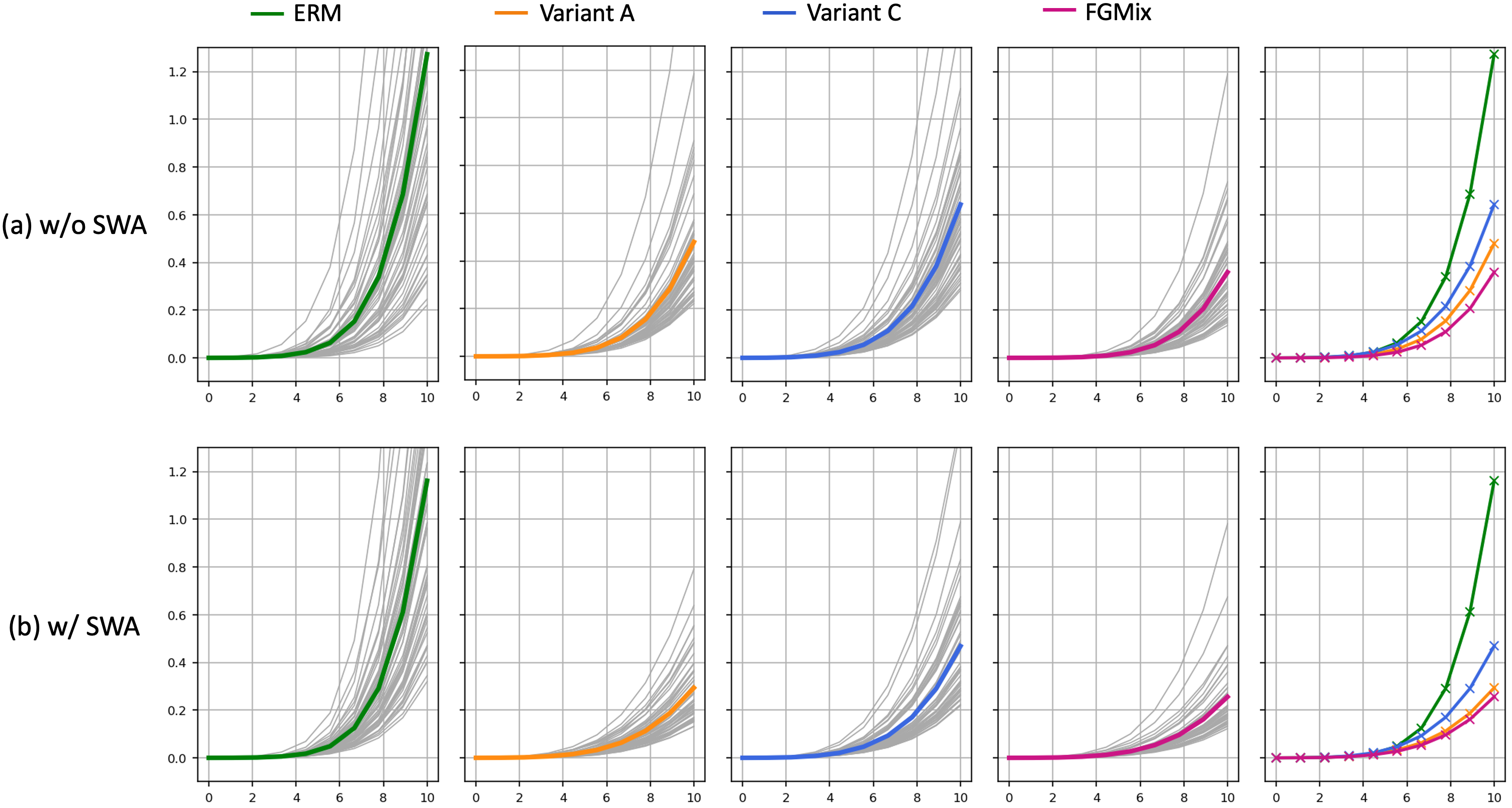
Figure 7: Target: L100; Source: L38, L43, L46.

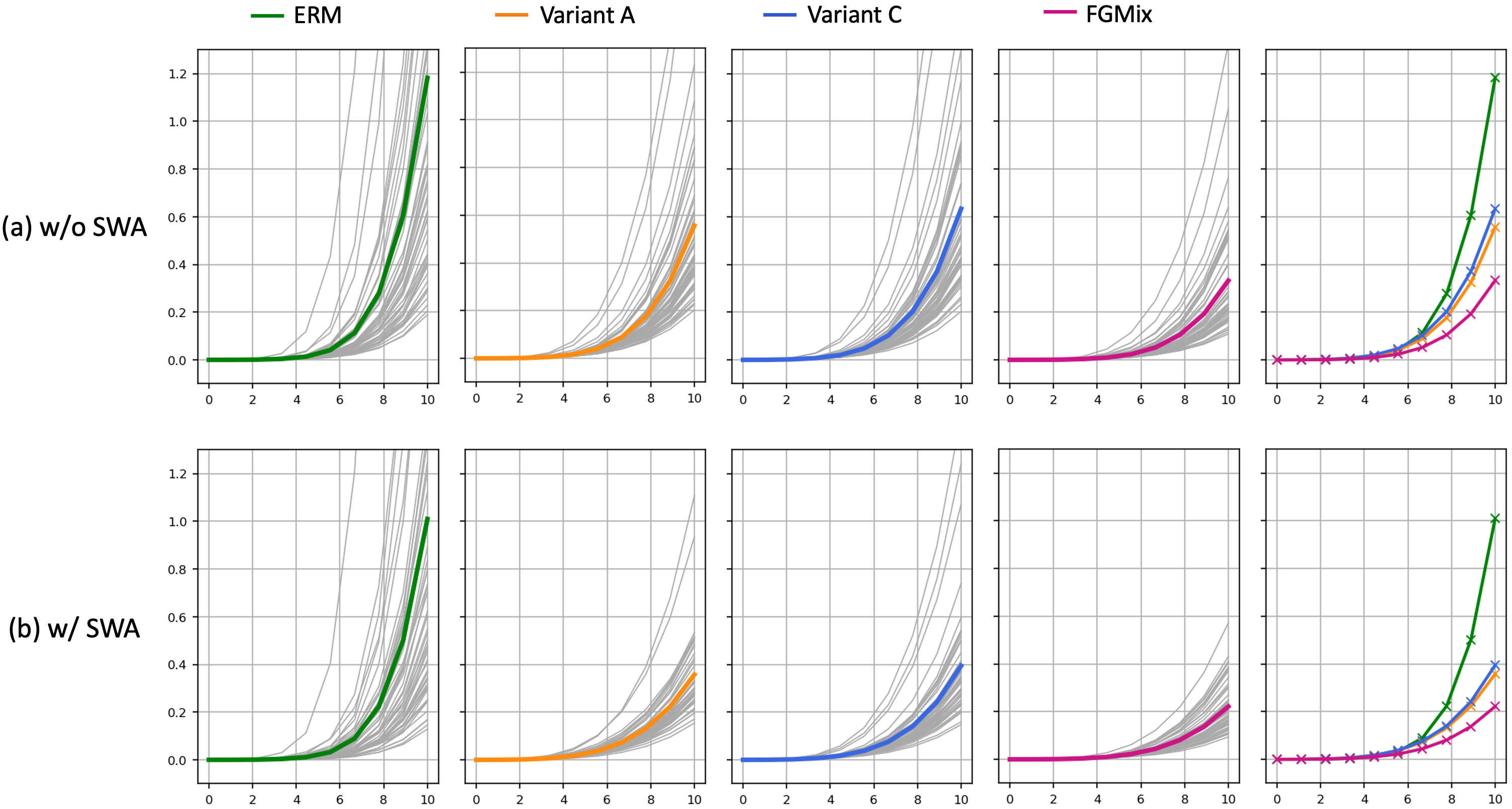
Figure 8: Target: L38; Source: L100, L43, L46.

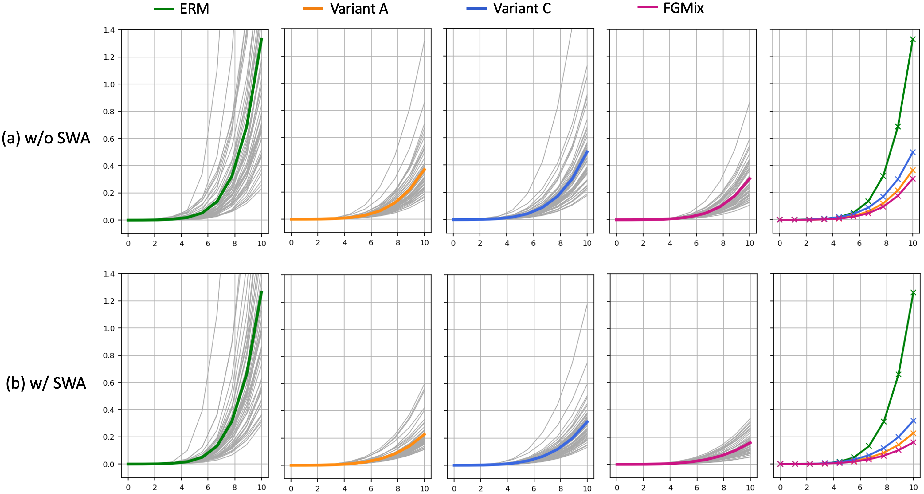
Figure 9: Target: L43; Source: L100, L38, L46.

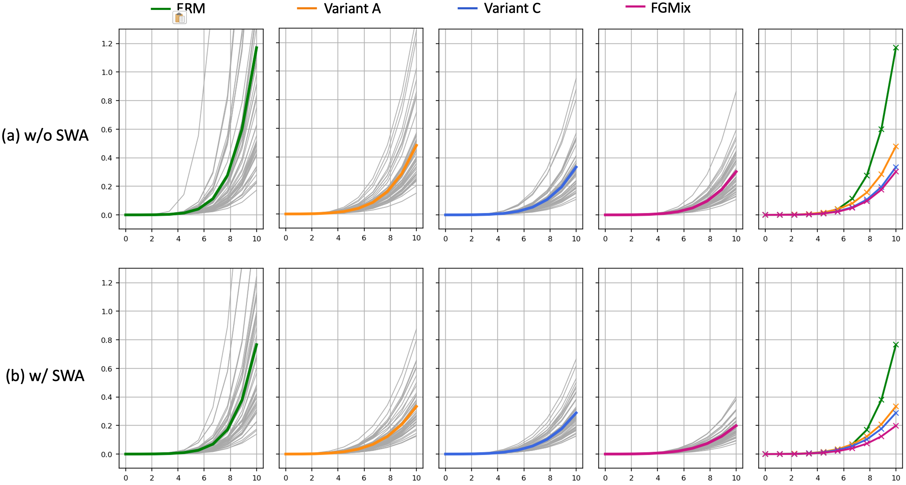
Figure 10: Target: L46; Source: L100, L38, L43.

A.3.2 Loss Surface & Optimization Path

To observe how the generated data affects the optimization process, we plot the 2D loss surface of the original training data (i.e., ERM) and the one after adding the generated mixup data (i.e., FGMix). We also plot the accuracy surface of the test data to visualize the distribution shift from the training domains. Since we include the mixup data for training only at the later stage of training, ERM and FGMix share the same optimization path at the beginning.

Figures 11-14 show the results when the test domain is L100, L38, L43 and L46 respectively. For test domain L100 and L38 (shown by Figure 11 and 12), we observe clear shift in optimum between the ERM train loss surface and the test accuracy surface. In this case, the narrow minima of ERM train loss surface is unable to cover the maxima of test accuracy surface. On the other hand, FGMix train loss surface yields wider and flatter minima, which better cover the test maxima. As a result, FGMix + SWA converges to a region with better test performance than ERM + SWA. Even for the case where the distribution shift is not significant (for test domain L43 and L46 shown by Figure 13 and 14 respectively), we observe that widening of the loss minima with FGMix will not cause harm to the optimization results, as both ERM + SWA and FGMix + SWA converge to a region with high test performance.

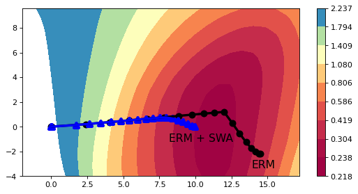
(a) ERM Train Loss Surface

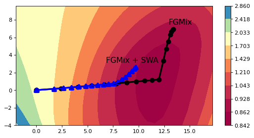
(b) FGMix Train Loss Surface

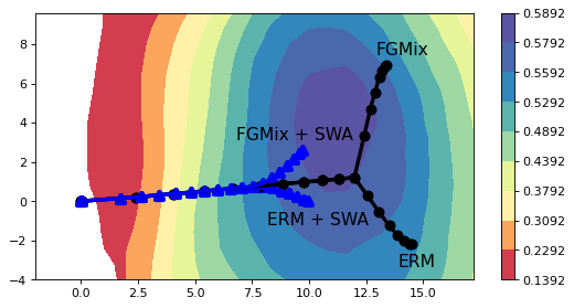
(c) Test Accuracy Surface

Figure 11: Target: L100; Source: L38, L43, L46.

(a) ERM Train Loss Surface

(b) FGMix Train Loss Surface

(c) Test Accuracy Surface

Figure 12: Target: L38; Source: L100, L43, L46.

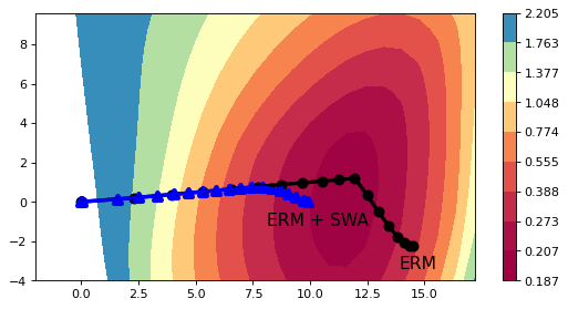
(a) ERM Train Loss Surface

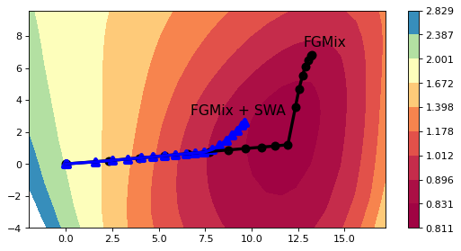
(b) FGMix Train Loss Surface

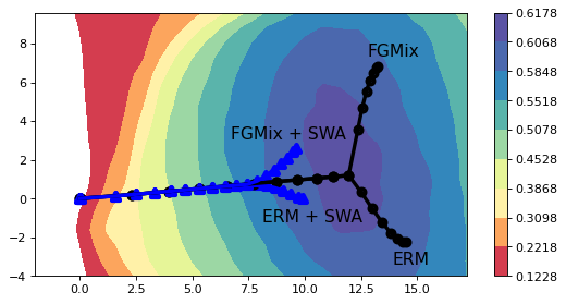
(c) Test Accuracy Surface

Figure 13: Target: L43; Source: L100, L38, L46.

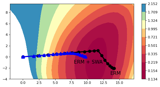
(a) ERM Train Loss Surface

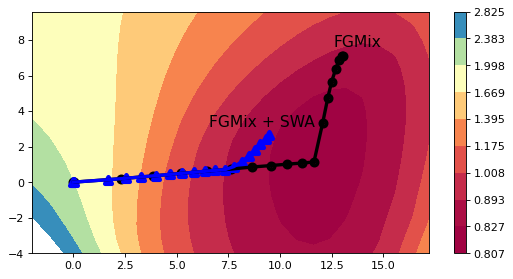
(b) FGMix Train Loss Surface

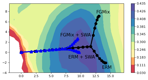
(c) Test Accuracy Surface

Figure 14: Target: L46; Source: L100, L38, L43.

A.4 2D Loss/Accuracy Surface Construction

Following Izmailov et al. [18], Cha et al. [6], we select 3 model weights $\{w_{1},w_{2},w_{3}\}$ at the initialization, the end of ERM + SWA optimization path, and the end of FGMix + SWA optimization path, respectively. Note that $w_{i}$ is the concatenation of vectorized $\theta_{i}$ and $\phi_{i}$ for the $i$-th selected model. We define the orthogonal basis $\{u,v\}$ of the 2D plane as:

$$u=w_{2}-w_{1},\ \ \ \ v=\frac{(w_{3}-w_{1})-\langle w_{3}-w_{1},w_{2}-w_{1}\rangle}{\|w_{2}-w_{1}\|^{2}\cdot(w_{2}-w_{1})}.$$

The orthonormal basis of the 2D plane is $\hat{u}=u/\|u\|$ and $\hat{v}=v/\|v\|$.

We project the optimization path onto the 2D plane by computing the coordinates of each point on the path. That is, for the point at the $j$-th step, its $u$- and $v$-coordinates are $\langle(w_{j}-w_{1}),\hat{u}\rangle$ and $\langle(w_{j}-w_{1}),\hat{v}\rangle$ respectively. To plot the loss surface, we define ranges on $u$- and $v$-axes that fully contain the optimization paths, say $[u_{1},u_{2}]$ for $u$-axis and $[v_{1},v_{2}]$ for $v$-axis. We then obtain the model weight corresponding to each grid point in the defined range, i.e., $w=w_{1}+a\hat{u}+b\hat{v}$, $\forall a\in[u_{1},u_{2}],b\in[v_{1},v_{2}]$, and compute the loss/accuracy of the entire training/test dataset using the model weight. The loss/accuracy values are visualized with a contour plot. For direct comparison, we use the same $u,v$ ranges for all three plots (ERM & FGMix train loss plots and test accuracy plot), and set the scale interval to be the same for the two train loss plots for flatness comparison.

A.5 Experiments on the Monte-Carlo Sample Size for the Flatness-Aware Objective

To optimize the flatness-aware objective, we propose to sample 100 directions to approximately measure the flatness in the model’s neighbourhoods. This involves computing the forward pass to the final classification layer for 100 times at each iteration, which contributes to the bulk of the computational cost of FGMix. To investigate whether this number can be further reduced to save cost, we vary the sample size in {10, 30, 50, 80, 100, 150, 200} and test the performance of FGMix (w/o SWA) on PACS. We conduct 5 trials for each case and report the mean values. The results are shown in Table 12.

Table 12: Effects of varying the sample size for FGMix on PACS (w/o SWA).

Sample Size	A	C	P	S	Avg.
10	86.3$\pm$0.8	79.7$\pm$1.0	97.6$\pm$1.1	80.2$\pm$1.0	86.0
30	87.0$\pm$1.1	79.2$\pm$1.3	97.7$\pm$0.9	80.1$\pm$1.2	86.0
50	87.2$\pm$1.3	80.4$\pm$1.3	97.8$\pm$0.6	80.5$\pm$1.1	86.5
80	86.9$\pm$1.3	81.7$\pm$0.9	97.8$\pm$0.7	80.4$\pm$1.2	86.7
100	87.2$\pm$1.0	81.2$\pm$1.0	97.9$\pm$0.8	80.2$\pm$1.4	86.6
150	87.3$\pm$0.8	80.6$\pm$1.1	97.6$\pm$1.0	81.0$\pm$0.8	86.6
200	87.2$\pm$0.7	81.4$\pm$0.8	97.8$\pm$0.6	80.7$\pm$0.9	86.8

From the results, we can see that the performance improvements from 10 to 150 are +0.0pp, +0.5pp, +0.2pp, -0.1pp, +0.0pp, +0.2pp respectively. The largest performance gain is from 30 to 50, after that the improvements seem to be minor. Hence, to save computational cost, we may consider reduce the sample size from 100 to 50 without serious compromise on the performance. Nevertheless, in this specific case, the best trade-off between efficiency and performance is to have a sample size of 80.

Appendix B Hyper-Parameters Settings

For our FGMix and all the reproduced algorithms (except for DDG, which will be detailed later), we set the batch size as 32 (due to constraint in computational resources), and tune dropout rate in {0, 0.1, 0.5}, learning rate in {1e-5, 3e-5, 5e-5} and weight decay in {1e-4, 1e-6}, following Cha et al. [6].

We reproduced 7 baselines (i.e., Manifold Mixup [42], MixStyle [49], MetaMixup [27], PCGrad [44], L2A-OT [48], CNSN [39] and DDG [47]) due to their lack of results on DomainBed benchmark [13]. We directly adopt the official implementations released by the respective authors into the DomainBed environment (refer to appendix of Gulrajani and Lopez-Paz [13] for how to incorporate new algorithms into DomainBed).

For Manifold Mixup, we set $\alpha=0.2$ for beta distribution from which the interpolation constant is sampled. For MixStyle, we set $\alpha=0.1$ for beta distribution and $p=0.5$ for the probability of applying MixStyle. As recommended, we insert the MixStyle layer after the 1st and 2nd residual blocks. For MetaMixup, we set the learning rate for the interpolation constant to 1e-3 (similar to our weight generation policy). PCGrad is free of additional hyper-parameters. For L2A-OT, we adopt ResNet-50 for both the classifier and the domain discriminator used to compute the domain divergence. Following the suggestions by the authors, we search $\lambda_{\text{Domain}}$ in {0.5, 1, 2}, $\lambda_{\text{Cycle}}$ in {10, 20} and $\lambda_{\text{CE}}$ in {1}. For CNSN, we apply both CrossNorm (2-instance mode) and SelfNorm and insert them at the end of each residual block of ResNet-50. Following the suggestions, we set the number of active CrossNorm layers to 1 and the probability to apply CrossNorm to 0.5 to avoid over data augmentation. For DDG, a 2-stage procedure is adopted, where the generator is pre-trained as a part of GANs in the first stage, and applied (and further updated) in the second stage. Following the official implementation, the batch size is set to 2 and the number of training steps is enlarged to 25,000 for the first stage and 10,000 for the second stage. Due to the 2-stage training and larger number of training steps, DDG takes a much longer time to train as compared to other baselines, making it less superior.

For our proposed FGMix, we set the iteration $\tau$ to start training and applying weight generation as 3,000, and the learning rate for weight generation policy $\beta$ as 1e-3. We tune the scaling factor $\lambda$ from {1, 3, 5, 10, 20}, the neighbourhood size $\gamma$ from $10^{\text{Uniform}(0,2)}$ and the size of generated mixup data as a multiple of the batch size from {1, 3, 5}. Regarding the network architecture, we use a 2-layer MLP for the similarity function $\mathcal{A}_{\omega}$ accompanied with $\tanh$ activation. The hidden sizes for both layers are set to 64. The discriminator $d$ is also a 2-layer MLP with hidden size 64. To apply SWA, we follow Arpit et al. [1] which suggests skipping the first few iterations and start applying weight averaging from the 100-th iteration.

References

- Arpit et al. [2021] Devansh Arpit, Huan Wang, Yingbo Zhou, and Caiming Xiong. Ensemble of averages: Improving model selection and boosting performance in domain generalization. arXiv preprint arXiv:2110.10832, 2021.
- Balaji et al. [2018] Yogesh Balaji, Swami Sankaranarayanan, and Rama Chellappa. Metareg: towards domain generalization using meta-regularization. In Proceedings of the 32nd International Conference on Neural Information Processing Systems, pages 1006–1016, 2018.
- Beery et al. [2018] Sara Beery, Grant Van Horn, and Pietro Perona. Recognition in terra incognita. In Proceedings of the European conference on computer vision (ECCV), pages 456–473, 2018.
- Berthelot et al. [2018] David Berthelot, Colin Raffel, Aurko Roy, and Ian Goodfellow. Understanding and improving interpolation in autoencoders via an adversarial regularizer. In International Conference on Learning Representations, 2018.
- Blanchard et al. [2011] Gilles Blanchard, Gyemin Lee, and Clayton Scott. Generalizing from several related classification tasks to a new unlabeled sample. Advances in neural information processing systems, 24, 2011.
- Cha et al. [2021] Junbum Cha, Sanghyuk Chun, Kyungjae Lee, Han-Cheol Cho, Seunghyun Park, Yunsung Lee, and Sungrae Park. Swad: Domain generalization by seeking flat minima. In Advances in Neural Information Processing Systems, 2021.
- Chapelle et al. [2000] Olivier Chapelle, Jason Weston, Léon Bottou, and Vladimir Vapnik. Vicinal risk minimization. In NIPS, 2000.
- Chaudhari et al. [2019] Pratik Chaudhari, Anna Choromanska, Stefano Soatto, Yann LeCun, Carlo Baldassi, Christian Borgs, Jennifer Chayes, Levent Sagun, and Riccardo Zecchina. Entropy-sgd: Biasing gradient descent into wide valleys (international conference on learning representations, iclr 2017). In 5th International Conference on Learning Representations, ICLR 2017, 2019.
- Chou et al. [2020] Hsin-Ping Chou, Shih-Chieh Chang, Jia-Yu Pan, Wei Wei, and Da-Cheng Juan. Remix: rebalanced mixup. In European Conference on Computer Vision, pages 95–110. Springer, 2020.
- Fang et al. [2013] Chen Fang, Ye Xu, and Daniel N Rockmore. Unbiased metric learning: On the utilization of multiple datasets and web images for softening bias. In Proceedings of the IEEE International Conference on Computer Vision, pages 1657–1664, 2013.
- Foret et al. [2020] Pierre Foret, Ariel Kleiner, Hossein Mobahi, and Behnam Neyshabur. Sharpness-aware minimization for efficiently improving generalization. In International Conference on Learning Representations, 2020.
- Garipov et al. [2018] T Garipov, P Izmailov, AG Wilson, D Podoprikhin, and D Vetrov. Loss surfaces, mode connectivity, and fast ensembling of dnns. In Advances in Neural Information Processing Systems, pages 8789–8798, 2018.
- Gulrajani and Lopez-Paz [2020] Ishaan Gulrajani and David Lopez-Paz. In search of lost domain generalization. arXiv preprint arXiv:2007.01434, 2020.
- Guo et al. [2019] Hongyu Guo, Yongyi Mao, and Richong Zhang. Mixup as locally linear out-of-manifold regularization. In Proceedings of the AAAI Conference on Artificial Intelligence, volume 33, pages 3714–3722, 2019.
- Guo et al. [2022] Hao Guo, Jiyong Jin, and Bin Liu. Stochastic weight averaging revisited. arXiv preprint arXiv:2201.00519, 2022.
- He et al. [2016] Kaiming He, Xiangyu Zhang, Shaoqing Ren, and Jian Sun. Deep residual learning for image recognition. In Proceedings of the IEEE conference on computer vision and pattern recognition, pages 770–778, 2016.
- Hochreiter et al. [1997] Sepp Hochreiter, J urgen Schmidhuber, and Corso Elvezia. Flat minima. Neural Computation, 9(1):1–42, 1997.
- Izmailov et al. [2018] P Izmailov, AG Wilson, D Podoprikhin, D Vetrov, and T Garipov. Averaging weights leads to wider optima and better generalization. In 34th Conference on Uncertainty in Artificial Intelligence 2018, UAI 2018, pages 876–885, 2018.
- Jiang et al. [2019] Yiding Jiang, Behnam Neyshabur, Hossein Mobahi, Dilip Krishnan, and Samy Bengio. Fantastic generalization measures and where to find them. In International Conference on Learning Representations, 2019.
- Keskar et al. [2017] Nitish Shirish Keskar, Jorge Nocedal, Ping Tak Peter Tang, Dheevatsa Mudigere, and Mikhail Smelyanskiy. On large-batch training for deep learning: Generalization gap and sharp minima. In 5th International Conference on Learning Representations, ICLR 2017, 2017.
- Kim et al. [2021] Daehee Kim, Youngjun Yoo, Seunghyun Park, Jinkyu Kim, and Jaekoo Lee. Selfreg: Self-supervised contrastive regularization for domain generalization. In Proceedings of the IEEE/CVF International Conference on Computer Vision, pages 9619–9628, 2021.
- Li et al. [2017] Da Li, Yongxin Yang, Yi-Zhe Song, and Timothy M Hospedales. Deeper, broader and artier domain generalization. In Proceedings of the IEEE international conference on computer vision, pages 5542–5550, 2017.
- Li et al. [2018a] Da Li, Yongxin Yang, Yi-Zhe Song, and Timothy M Hospedales. Learning to generalize: Meta-learning for domain generalization. In Thirty-Second AAAI Conference on Artificial Intelligence, 2018.
- Li et al. [2018b] Haoliang Li, Sinno Jialin Pan, Shiqi Wang, and Alex C Kot. Domain generalization with adversarial feature learning. In Proceedings of the IEEE Conference on Computer Vision and Pattern Recognition, pages 5400–5409, 2018.
- Li et al. [2019] Da Li, Jianshu Zhang, Yongxin Yang, Cong Liu, Yi-Zhe Song, and Timothy M Hospedales. Episodic training for domain generalization. In Proceedings of the IEEE/CVF International Conference on Computer Vision, pages 1446–1455, 2019.
- MacKay [1992] David JC MacKay. A practical bayesian framework for backpropagation networks. Neural Computation, 4(3):448–472, 1992.
- Mai et al. [2021] Zhijun Mai, Guosheng Hu, Dexiong Chen, Fumin Shen, and Heng Tao Shen. Metamixup: Learning adaptive interpolation policy of mixup with metalearning. IEEE Transactions on Neural Networks and Learning Systems, 2021.
- Mansilla et al. [2021] Lucas Mansilla, Rodrigo Echeveste, Diego H Milone, and Enzo Ferrante. Domain generalization via gradient surgery. In Proceedings of the IEEE/CVF International Conference on Computer Vision, pages 6630–6638, 2021.
- Muandet et al. [2013] Krikamol Muandet, David Balduzzi, and Bernhard Schölkopf. Domain generalization via invariant feature representation. In International Conference on Machine Learning, pages 10–18. PMLR, 2013.
- Nam et al. [2021] Hyeonseob Nam, HyunJae Lee, Jongchan Park, Wonjun Yoon, and Donggeun Yoo. Reducing domain gap by reducing style bias. In Proceedings of the IEEE/CVF Conference on Computer Vision and Pattern Recognition, pages 8690–8699, 2021.
- Parascandolo et al. [2020] Giambattista Parascandolo, Alexander Neitz, ANTONIO ORVIETO, Luigi Gresele, and Bernhard Schölkopf. Learning explanations that are hard to vary. In International Conference on Learning Representations, 2020.
- Peng et al. [2019] Xingchao Peng, Qinxun Bai, Xide Xia, Zijun Huang, Kate Saenko, and Bo Wang. Moment matching for multi-source domain adaptation. In Proceedings of the IEEE/CVF international conference on computer vision, pages 1406–1415, 2019.
- Petzka et al. [2021] Henning Petzka, Michael Kamp, Linara Adilova, Cristian Sminchisescu, and Mario Boley. Relative flatness and generalization. In Advances in Neural Information Processing Systems, 2021.
- Rame et al. [2021] Alexandre Rame, Corentin Dancette, and Matthieu Cord. Fishr: Invariant gradient variances for out-of-distribution generalization. arXiv preprint arXiv:2109.02934, 2021.
- Riemer et al. [2018] Matthew Riemer, Ignacio Cases, Robert Ajemian, Miao Liu, Irina Rish, Yuhai Tu, and Gerald Tesauro. Learning to learn without forgetting by maximizing transfer and minimizing interference. In International Conference on Learning Representations, 2018.
- Shahtalebi et al. [2021] Soroosh Shahtalebi, Jean-Christophe Gagnon-Audet, Touraj Laleh, Mojtaba Faramarzi, Kartik Ahuja, and Irina Rish. Sand-mask: An enhanced gradient masking strategy for the discovery of invariances in domain generalization. arXiv preprint arXiv:2106.02266, 2021.
- Shi et al. [2021] Yuge Shi, Jeffrey Seely, Philip HS Torr, N Siddharth, Awni Hannun, Nicolas Usunier, and Gabriel Synnaeve. Gradient matching for domain generalization. arXiv preprint arXiv:2104.09937, 2021.
- Sun and Saenko [2016] Baochen Sun and Kate Saenko. Deep coral: Correlation alignment for deep domain adaptation. In European conference on computer vision, pages 443–450. Springer, 2016.
- Tang et al. [2021] Zhiqiang Tang, Yunhe Gao, Yi Zhu, Zhi Zhang, Mu Li, and Dimitris N Metaxas. Crossnorm and selfnorm for generalization under distribution shifts. In Proceedings of the IEEE/CVF International Conference on Computer Vision, pages 52–61, 2021.
- Vapnick [1998] Vladimir N Vapnick. Statistical learning theory. Wiley, New York, 1998.
- Venkateswara et al. [2017] Hemanth Venkateswara, Jose Eusebio, Shayok Chakraborty, and Sethuraman Panchanathan. Deep hashing network for unsupervised domain adaptation. In Proceedings of the IEEE conference on computer vision and pattern recognition, pages 5018–5027, 2017.
- Verma et al. [2019] Vikas Verma, Alex Lamb, Christopher Beckham, Amir Najafi, Ioannis Mitliagkas, David Lopez-Paz, and Yoshua Bengio. Manifold mixup: Better representations by interpolating hidden states. In International Conference on Machine Learning, pages 6438–6447. PMLR, 2019.
- Wang et al. [2020] Yufei Wang, Haoliang Li, and Alex C Kot. Heterogeneous domain generalization via domain mixup. In ICASSP 2020-2020 IEEE International Conference on Acoustics, Speech and Signal Processing (ICASSP), pages 3622–3626. IEEE, 2020.
- Yu et al. [2020] Tianhe Yu, Saurabh Kumar, Abhishek Gupta, Sergey Levine, Karol Hausman, and Chelsea Finn. Gradient surgery for multi-task learning. Advances in Neural Information Processing Systems, 33:5824–5836, 2020.
- Yun et al. [2019] Sangdoo Yun, Dongyoon Han, Seong Joon Oh, Sanghyuk Chun, Junsuk Choe, and Youngjoon Yoo. Cutmix: Regularization strategy to train strong classifiers with localizable features. In Proceedings of the IEEE/CVF international conference on computer vision, pages 6023–6032, 2019.
- Zhang et al. [2018] Hongyi Zhang, Moustapha Cisse, Yann N Dauphin, and David Lopez-Paz. mixup: Beyond empirical risk minimization. In International Conference on Learning Representations, 2018.
- Zhang et al. [2022] Hanlin Zhang, Yi-Fan Zhang, Weiyang Liu, Adrian Weller, Bernhard Schölkopf, and Eric P Xing. Towards principled disentanglement for domain generalization. In Proceedings of the IEEE/CVF Conference on Computer Vision and Pattern Recognition, pages 8024–8034, 2022.
- Zhou et al. [2020a] Kaiyang Zhou, Yongxin Yang, Timothy Hospedales, and Tao Xiang. Learning to generate novel domains for domain generalization. In European conference on computer vision, pages 561–578. Springer, 2020.
- Zhou et al. [2020b] Kaiyang Zhou, Yongxin Yang, Yu Qiao, and Tao Xiang. Domain generalization with mixstyle. In International Conference on Learning Representations, 2020.