The Helmholtz equation with uncertainties in the wavenumber

Abstract

We investigate the Helmholtz equation with suitable boundary conditions and uncertainties in the wavenumber. Thus the wavenumber is modeled as a random variable or a random field. We discretize the Helmholtz equation using finite differences in space, which leads to a linear system of algebraic equations including random variables. A stochastic Galerkin method yields a deterministic linear system of algebraic equations. This linear system is high-dimensional, sparse and complex symmetric but, in general, not hermitian. We therefore solve this system iteratively with GMRES and propose two preconditioners: a complex shifted Laplace preconditioner and a mean value preconditioner. Both preconditioners reduce the number of iteration steps as well as the computation time in our numerical experiments.

Keywords:

Helmholtz equation, polynomial chaos, stochastic Galerkin method, GMRES, complex shifted Laplace preconditioner, mean value preconditioner

AMS Subject Classification (2020):

65N30, 65C20, 35R60

1 Introduction

The Helmholtz equation is a linear partial differential equation (PDE), whose solutions are time-harmonic states of the wave equation, see [14, 19]. Important applications of this model are given in acoustics and electromagnetics [2]. The Helmholtz equation includes a wavenumber, which is either a constant parameter or a space-dependent function. Furthermore, boundary conditions are imposed on the spatial domain.

We consider uncertainties in the wavenumber. Thus the wavenumber is replaced by a random variable or a spatial random field to quantify the uncertainties. The solution of the Helmholtz equation changes into a random field, which can be expanded into the (generalized) polynomial chaos, see [30]. We employ the stochastic Galerkin method to compute approximations of the unknown coefficient functions. Stochastic Galerkin methods were used for linear PDEs of different types including random variables, for example, see [12, 32] on elliptic type, [13, 22] on hyperbolic type, and [21, 31] on parabolic type. Wang et al. [29] applied a multi-element stochastic Galerkin method to solve the Helmholtz equation including random variables. We investigate the ordinary stochastic Galerkin method, which is efficient if the wavenumbers are not close to resonance.

The stochastic Galerkin method transforms the random-dependent Helmholtz equation into a deterministic system of linear PDEs. Likewise, the original boundary conditions yield boundary conditions for this system. We examine the system of PDEs in one and two space dimensions. A finite difference method, see [15], produces a high-dimensional linear system of algebraic equations. When considering absorbing boundary conditions, the coefficient matrices are complex-valued and non-hermitian.

We focus on the numerical solution of the linear systems of algebraic equations. The dimension of these linear systems rapidly grows for increasing numbers of random variables. Hence we use iterative methods like GMRES [24] in the numerical solution. The efficiency of an iterative method strongly depends on an appropriate preconditioning of the linear systems. We propose two preconditioners in the general case where the wavenumber can depend on space and on multiple random variables: a complex shifted Laplace preconditioner, see [6, 8], and a mean value preconditioner, see [10, 29]. Statements on the location of spectra and estimates of matrix norms are shown. Furthermore, results of numerical computations are presented for both settings.

The article is organized as follows. The stochastic Helmholtz equation is introduced in Section 2 and discretized in Section 3. We discuss the complex shifted Laplace preconditioner in Section 4 and the mean value preconditioner in Section 5. Sections 6 and 7 contain numerical experiments in one and two spatial dimensions, respectively, which show the effectiveness of the preconditioners. An appendix includes the detailed formulas of the discretizations in space.

2 Problem Definition

We illustrate the stochastic problem associated to the Helmholtz equation.

2.1 Helmholtz equation

The Helmholtz equation is a PDE of the form

$$-\Delta u-k^{2}u=f\quad\text{in }Q$$ (2.1)

with an (open) spatial domain $Q\subseteq\mathbb{R}^{d}$ and given source term $f:Q\to\mathbb{R}$. The wavenumber $k$ is either a positive constant or a function $k:\overline{Q}\rightarrow\mathbb{R}_{+}$. The unknown solution is $u:\overline{Q}\rightarrow\mathbb{K}$ with either $\mathbb{K}=\mathbb{R}$ or $\mathbb{K}=\mathbb{C}$. Here $\Delta=\sum_{j=1}^{d}\frac{\partial^{2}}{\partial x_{j}^{2}}$ denotes the Laplace operator with respect to $x=[x_{1},\ldots,x_{d}]^{\top}\in\mathbb{R}^{d}$.

Often homogeneous Dirichlet boundary conditions, i.e.,

$$u=0\quad\text{on }\partial Q,$$ (2.2)

are applied for simplicity. Alternatively, absorbing boundary conditions read as

$$\partial_{n}u-{\operatorname{i}}ku=0\quad\text{on }\partial Q,$$ (2.3)

where $\partial_{n}$ denotes the derivative with respect to the outward normal of $Q$ and ${\operatorname{i}}=\sqrt{-1}$ is the imaginary unit.

2.2 Stochastic modeling

We consider uncertainties in the wavenumber. A simple model to include a variation of the wavenumber is to replace the constant $k$ by a random variable on a probability space $(\Omega,\mathcal{A},P)$. We write $k=k(\xi)$, where $\xi:\Omega\rightarrow\mathbb{R}$ is some random variable with a traditional probability distribution. More generally, the wavenumber can be a space-dependent function on $\overline{Q}$ including a multidimensional random variable $\xi:\Omega\rightarrow\Xi$ with $\Xi\subseteq\mathbb{R}^{s}$. We assume $\xi=(\xi_{1},\ldots,\xi_{s})^{\top}$ with independent random variables $\xi_{\ell}$ for $\ell=1,\ldots,s$. Now the wavenumber becomes a random field

$$k(x,\xi)=k_{0}(x)+\sum_{\ell=1}^{s}\xi_{\ell}k_{\ell}(x)$$ (2.4)

with given functions $k_{\ell}:\overline{Q}\rightarrow\mathbb{R}$ for $\ell=0,1,\ldots,s$, as in [29]. A truncation of a Karhunen-Loève expansion, see [11, p. 17], also yields a random input of the form (2.4). Consequently, the solution of the deterministic Helmholtz equation (2.1) changes into a random field $u:\overline{Q}\times\Xi\rightarrow\mathbb{K}$. We write $u(x,\xi)$ to indicate the dependence of the solution on space as well as the random variables.

We assume that each random variable $\xi_{\ell}$ has a probability density function $\rho_{\ell}$. Since the random variables are independent, the product $\rho=\rho_{1}\cdots\rho_{s}$ is the joint probability density function. Without loss of generality, let $\rho(\xi)>0$ for almost all $\xi\in\Xi$. The expected value of a measurable function $f:\Xi\rightarrow\mathbb{K}$ depending on the random variables is

$$\mathbb{E}(f)=\int_{\Omega}f(\xi(\omega))\;\textrm{d}P(\omega)=\int_{\Xi}f(\xi)\,\rho(\xi)\,\textrm{d}\xi,$$

if the integral exists. The inner product of two square-integrable functions $f,g$ is

$$\langle f,g\rangle=\int_{\Xi}f(\xi)\,\overline{g(\xi)}\,\rho(\xi)\,\textrm{d}\xi.$$ (2.5)

In the following, $\mathcal{L}^{2}(\Xi,\rho)$ denotes the Hilbert space of square-integrable functions. The associated norm is $\lVert f\rVert_{\mathcal{L}^{2}(\Xi,\rho)}=\sqrt{\langle f,f\rangle}$.

Later we will focus on uniformly distributed random variables $\xi_{\ell}:\Omega\to[-1,1]$. In this case, the joint probability density function is constant, i.e., $\Xi=[-1,1]^{s}$ and $\rho\equiv 2^{-s}$.

2.3 Polynomial chaos expansions

We assume that there is an orthonormal polynomial basis $(\phi_{i})_{i\in\mathbb{N}_{0}}$ in $\mathcal{L}^{2}(\Xi,\rho)$. Thus it holds that

$$\langle\phi_{i},\phi_{j}\rangle=\delta_{i,j}=\begin{cases}1&\text{for }i=j\\ 0&\text{for }i\neq j\\ \end{cases}$$

with the inner product (2.5). In the case of uniform probability distributions, the multivariate functions $\phi_{i}$ are products of the (univariate) Legendre polynomials. We assume that $\phi_{0}\equiv 1$. The number $m+1$ of multivariate polynomials in $s$ variables up to a total degree $r$ is

$$m+1=\frac{(s+r)!}{s!\,r!},$$ (2.6)

see [30, p. 65]. This number grows fast for increasing $r$ or $s$.

Let $u(x,\cdot)\in\mathcal{L}^{2}(\Xi,\rho)$ for each $x\in\overline{Q}$. The polynomial chaos (PC) expansion is

$$u(x,\xi)=\sum_{i=0}^{\infty}v_{i}(x)\phi_{i}(\xi)$$ (2.7)

with (a priori unknown) coefficient functions

$$v_{i}(x)=\langle u(x,\xi),\phi_{i}(\xi)\rangle\quad\text{for }i\in\mathbb{N}_{0}.$$ (2.8)

The series (2.7) converges in $\mathcal{L}^{2}(\Xi,\rho)$ pointwise for $x\in\overline{Q}$. If the wavenumber $k$ is an analytic function of the random variables, then the rate of convergence is exponentially fast for traditional probability distributions.

3 Discretization of the stochastic Helmholtz equation

We consider the stochastic Helmholtz equation

$$-\Delta u(x,\xi)-k(x,\xi)^{2}u(x,\xi)=f(x),\quad x\in Q\subseteq\mathbb{R}^{d},$$ (3.1)

with given source term $f:Q\to\mathbb{R}$ and random wavenumber $k:\overline{Q}\times\Xi\to\mathbb{R}_{+}$, together with either homogeneous Dirichlet boundary conditions

$$u(x,\xi)=0,\quad x\in\partial Q,\quad\xi\in\Xi,$$ (3.2)

or with absorbing boundary conditions

$$\partial_{n}u(x,\xi)-{\operatorname{i}}k(x,\xi)u(x,\xi)=0,\quad x\in\partial Q,\quad\xi\in\Xi.$$ (3.3)

All derivatives are taken with respect to $x$. We discretize this boundary value problem in two steps, with a finite difference method (FDM) in space and the stochastic Galerkin method in the random-dependent part. The steps can be done in any order. We first give an overview of the procedure when beginning with the FDM in Section 3.1. In Section 3.2, we discuss the discretization when beginning with the stochastic Galerkin method.

3.1 FDM and stochastic Galerkin method

A spatial discretization of the boundary value problem with a FDM leads to a (stochastic) linear algebraic system

$$S(\xi)U(\xi)=F_{0}$$ (3.4)

with $S(\xi)\in\mathbb{K}^{n,n}$ for $\xi\in\Xi$ (see Section A for details) and constant vector $F_{0}\in\mathbb{R}^{n}$. In a second step, we consider a PC approximation of $U(\xi)$ of the form

$$\widetilde{U}_{m}(\xi)=\sum_{i=0}^{m}\phi_{i}(\xi)V_{i},\quad\text{where }V_{i}=\begin{bmatrix}v_{\ell,i}\end{bmatrix}_{\ell=1}^{n}\in\mathbb{R}^{n}\text{ for }i=0,1,\ldots,m,$$ (3.5)

and $\phi_{i}$ are polynomials as in Section 2.3. The coefficient vectors $V_{i}$ are determined by the orthogonality of the residual

$$R_{m}(\xi)=S(\xi)\widetilde{U}_{m}(\xi)-F_{0}.$$ (3.6)

to the subspace $\operatorname{span}\{\phi_{0},\phi_{1},\ldots,\phi_{m}\}$ with respect to the inner product $\langle\cdot,\cdot\rangle$ in (2.5), i.e., by $\langle R_{m}(\xi),\phi_{i}(\xi)\rangle=0$ for $i=0,1,\ldots,m$. Here the inner product is taken component-wise. The orthogonality condition is equivalent to

$$\langle S(\xi)\widetilde{U}_{m}(\xi),\phi_{i}(\xi)\rangle=\langle 1,\phi_{i}(\xi)\rangle F_{0}=\delta_{i,0}F_{0},\quad i=0,1,\ldots,m,$$ (3.7)

due to $\phi_{0}\equiv 1$. This leads to a (deterministic) linear algebraic system

$$AV=F,\quad V=\begin{bmatrix}V_{0}\\ \vdots\\ V_{m}\end{bmatrix},\quad F=\begin{bmatrix}F_{0}\\ \vdots\\ F_{m}\end{bmatrix},$$ (3.8)

where the stochastic Galerkin projection $A\in\mathbb{K}^{(m+1)n,(m+1)n}$ is a block matrix with $m+1$ blocks of size $n\times n$, and $F_{i}=0\in\mathbb{R}^{n}$ for $i=1,\ldots,m$.

Remark 3.1.

The Galerkin approximation (3.5) can be interpreted as a spatial discretization of a Galerkin approximation $\widetilde{u}_{m}(x,\xi)=\sum_{i=0}^{m}v_{i}(x)\phi_{i}(\xi)$ of $u(x,\xi)$. Evaluating $\widetilde{u}_{m}$ at discretization points $x_{1},\ldots,x_{n}$ yields

$$\begin{bmatrix}\widetilde{u}_{m}(x_{1},\xi)\\ \vdots\\ \widetilde{u}_{m}(x_{n},\xi)\end{bmatrix}=\sum_{i=0}^{m}\phi_{i}(\xi)\begin{bmatrix}v_{i}(x_{1})\\ \vdots\\ v_{i}(x_{n})\end{bmatrix}.$$ (3.9)

Hence $V_{i}$ in (3.5) can be interpreted as a discretization of $v_{i}(x)$ by $v_{\ell,i}=v_{i}(x_{\ell})$.

As it turns out, the matrix $S(\xi)$ is a (complex) linear combination of symmetric positive (semi-)definite matrices. The following lemma shows that this structure is preserved in the stochastic Galerkin method; see [20, Lem. 1] and its proof. These properties of the matrix $S$ and thus $A$ will be essential for our analysis of shifted Laplace preconditioners in Section 4.

Lemma 3.2.

Let $A(\xi)=\begin{bmatrix}a_{\mu,\nu}(\xi)\end{bmatrix}_{\mu,\nu}\in\mathbb{R}^{n,n}$ with $a_{\mu,\nu}\in\mathcal{L}^{2}(\Xi,\rho)$, and $V\in\mathbb{R}^{n}$. Define

$$A_{ij}\coloneq\begin{bmatrix}\langle a_{\mu,\nu}(\xi)\phi_{i}(\xi),\phi_{j}(\xi)\rangle\end{bmatrix}_{\mu,\nu}\in\mathbb{R}^{n,n},\quad i,j=0,1,\ldots,m,$$ (3.10)

and the stochastic Galerkin projection

$$A\coloneq\begin{bmatrix}A_{ij}\end{bmatrix}_{i,j}\in\mathbb{R}^{(m+1)n,(m+1)n}.$$ (3.11)

We then obtain for $i,j=0,1,\ldots,m$

$$\langle A(\xi)\phi_{i}(\xi)V,\phi_{j}(\xi)\rangle=A_{ij}V,$$ (3.12)

where the inner product is taken component-wise. Additionally, $A_{ij}=A_{ji}$. Moreover, if $A(\xi)$ is symmetric, then $A$ is symmetric, and if $A(\xi)$ is symmetric positive (semi-)definite for almost all $\xi\in\Xi$ then $A$ is symmetric positive (semi-)definite.

Corollary 3.3.

In the notation of Lemma 3.2, if $A(\xi)=A_{0}$ is independent of $\xi$, then $A_{ij}=\delta_{ij}A_{0}$ and $A=I_{m+1}\otimes A_{0}$, with the identity matrix $I_{m+1}\in\mathbb{K}^{m+1,m+1}$ and the Kronecker product.

Finally, we obtain the following result on the structure of the matrix $A$ in (3.8).

Theorem 3.4.

Let the spatial dimension be $d\in\{1,2\}$. A finite difference and stochastic Galerkin approximation of the Helmholtz equation (3.1) with either homogeneous Dirichlet or absorbing boundary conditions leads to a linear system (3.8) with coefficient matrix

$$A=L-{\operatorname{i}}B-K$$ (3.13)

and real-valued matrices $L,B,K$. The matrix $K$ is symmetric positive definite, $B,L$ are symmetric positive semidefinite. In case of homogeneous Dirichlet boundary conditions, $L$ is symmetric positive definite and $B=0$.

Proof.

The FD discretizations leading to $S(\xi)U(\xi)=F_{0}$ in (3.4) are given in Section A. The statement of the theorem follows in each case by applying the stochastic Galerkin approximation as described above and using Lemma 3.2 as well as Corollary 3.3 separately for each term composing $S(\xi)$. ∎

The matrix $L$ results essentially from the discretization of the Laplacian, $B$ from the (absorbing) boundary conditions, and $K$ is the discretization of the term including the wavenumber; see Section A for details.

3.2 Stochastic Galerkin method and FDM

Alternatively, we can begin with the stochastic Galerkin method. This leads to a system of deterministic PDEs, which are subsequently discretized by a FDM. The PC expansion (2.7) suggests a stochastic Galerkin approximation of $u(x,\xi)$ of the form

$$\widetilde{u}_{m}(x,\xi)=\sum_{i=0}^{m}v_{i,m}(x)\phi_{i}(\xi).$$ (3.14)

The coefficient functions $v_{i,m}$ in the stochastic Galerkin method are in general distinct from the coefficients $v_{i}$ in (2.8). Nevertheless, we will usually write $v_{i}$ instead of $v_{i,m}$ in the sequel for notational convenience. The coefficients in the Galerkin approach are determined by the orthogonality of the residual

$$R_{m}(x,\xi) =-\Delta\widetilde{u}_{m}(x,\xi)-k(x,\xi)^{2}\widetilde{u}_{m}(x,\xi)-f(x)$$

$$=-\sum_{i=0}^{m}\Delta v_{i}(x)\phi_{i}(\xi)-k(x,\xi)^{2}\sum_{i=0}^{m}v_{i}(x)\phi_{i}(\xi)-f(x)$$

to the subspace $\operatorname{span}\{\phi_{0},\phi_{1},\ldots,\phi_{m}\}$, i.e., by $\langle R_{m}(x,\xi),\phi_{j}(\xi)\rangle=0$ for $j=0,1,\ldots,m$ and each $x\in Q$. The latter is equivalent to

$$-\Delta v_{j}(x)-\sum_{i=0}^{m}\langle k(x,\xi)^{2}\phi_{i}(\xi),\phi_{j}(\xi)\rangle v_{i}(x)=\langle 1,\phi_{j}(\xi)\rangle f(x)=\delta_{j,0}f(x)$$ (3.15)

for $j=0,1,\ldots,m$ in $Q$. Thus we obtain a system of PDEs for the unknown coefficient functions $v_{0},v_{1},\ldots,v_{m}$. Define $C(x)=[c_{ij}(x)]\in\mathbb{R}^{m+1,m+1}$ for $x\in Q$ by

$$c_{ij}(x)=\langle k(x,\xi)^{2}\phi_{i}(\xi),\phi_{j}(\xi)\rangle=\int_{\Xi}\phi_{i}(\xi)\phi_{j}(\xi)k(x,\xi)^{2}\rho(\xi)\,\textrm{d}\xi,\quad i,j=0,1,\ldots,m.$$ (3.16)

Since by assumption $k(x,\xi)>0$ for all $x$ and $\xi$, the matrix $C(x)$ is symmetric positive definite (as Gramian of an inner product with weight function $k(x,\xi)^{2}\rho(\xi)$). Setting

$$v(x)=\begin{bmatrix}v_{0}(x)&v_{1}(x)&\cdots&v_{m}(x)\end{bmatrix}^{\top},\quad F(x)=\begin{bmatrix}f(x)&0&\cdots&0\end{bmatrix}^{\top},$$ (3.17)

we write the system of PDEs (3.15) as

$$-\Delta v(x)-C(x)v(x)=F(x)\quad\text{in }Q,$$ (3.18)

which is a larger deterministic system of linear PDEs. Still we require boundary conditions for the system (3.18).

The homogeneous Dirichlet boundary condition (3.2) implies $v_{j}(x)=0$ for $x\in\partial Q$ and $j=0,1,\ldots,m$, hence

$$v(x)=0\quad\text{on }\partial Q.$$ (3.19)

Inserting the Galerkin approximation (3.14) into the absorbing boundary conditions (3.3) yields the residual

$$R_{m}(x,\xi) =\sum_{i=0}^{m}(\partial_{n}v_{i})(x)\phi_{i}(\xi)-{\operatorname{i}}k(x,\xi)\sum_{i=0}^{m}v_{i}(x)\phi_{i}(\xi).$$ (3.20)

By the orthogonality $\langle R_{m}(x,\xi),\phi_{j}(\xi)\rangle=0$ in the Galerkin approach, we obtain

$$\partial_{n}v_{j}(x)-{\operatorname{i}}\sum_{i=0}^{m}\langle k(x,\xi)\phi_{i}(\xi),\phi_{j}(\xi)\rangle v_{i}(x)=0,\quad j=0,1,\ldots,m.$$ (3.21)

The matrix $B(x)=[b_{ij}(x)]\in\mathbb{R}^{m+1,m+1}$ with

$$b_{ij}(x)=\langle k(x,\xi)\phi_{i}(\xi),\phi_{j}(\xi)\rangle=\int_{\Xi}\phi_{i}(\xi)\phi_{j}(\xi)k(x,\xi)\rho(\xi)\,\textrm{d}\xi,\quad i,j=0,1,\ldots,m,$$ (3.22)

is symmetric and positive definite (since $k(x,\xi)>0$ by assumption). The boundary condition (3.21) can be written with $B(x)$ as

$$(\partial_{n}v)(x)-{\operatorname{i}}B(x)v(x)=0\quad\text{on }\partial Q.$$ (3.23)

The boundary value problem (3.18) with (3.19) or (3.23) is discretized in Section A.4 (in dimension $d=1$). The resulting linear algebraic system is the same as the one obtained in Section 3.1.

4 Complex shifted Laplace preconditioner

Following the investigation in [9], we consider the Helmholtz equation (3.1) with a complex shift in the wavenumber

$$-\Delta u(x,\xi)-(1+{\operatorname{i}}\beta)k(x,\xi)^{2}u(x,\xi)=f(x),\quad x\in Q,$$ (4.1)

with $\beta\in\mathbb{R}$, together with either homogeneous Dirichlet boundary conditions (3.2) or absorbing boundary conditions (3.3). We discretize this boundary value problem as described in Section 3.1. For $\beta=0$, we have the matrix (3.13) in Theorem 3.4, and for $\beta\in\mathbb{R}$ we obtain

$$M\coloneq M(\beta)\coloneq L-{\operatorname{i}}B-(1+{\operatorname{i}}\beta)K=A-{\operatorname{i}}\beta K,$$ (4.2)

since only the constant term is multiplied by $1+{\operatorname{i}}\beta$. Motivated by [27, p. 1945], we call $M$ a complex shifted Laplace preconditioner (CSL preconditioner).

For the deterministic Helmholtz equation, preconditioning with the CSL preconditioner is a widely studied and successful technique for solving the discretized Helmholtz equation; see, e.g., [6, 1, 23, 3, 7] and [9], as well as references therein. See also [5] for a survey and [17] for recent developments. In the deterministic case, the spectrum of the preconditioned matrix $AM^{-1}$ lies in the disk (4.3), and the improved localization of the spectrum typically leads to a faster convergence of Krylov solvers. The CSL preconditioner $M$ can be inverted efficiently, for example, by multigrid techniques.

Here, we focus on locating the spectrum of the preconditioned matrix in the stochastic case, in analogy to [27, 8, 9] for the deterministic Helmholtz equation.

Theorem 4.1.

Let the notation be as in Theorem 3.4, let $\beta>0$, let $A$ be the discretization (3.13) of the stochastic Helmholtz equation (3.1) and $M$ be the discretization (4.2) of the shifted Helmholtz equation (4.1).

1. In the case of absorbing boundary conditions (3.3), the spectrum of the preconditioned matrix $AM^{-1}$ is contained in the closed disk

   $$\mathcal{D}=\{z\in\mathbb{C}:\lvert z-1/2\rvert\leq 1/2\}.$$ (4.3)

2. In the case of homogeneous Dirichlet boundary conditions (3.2), the spectrum of the preconditioned matrix $AM^{-1}$ lies on the circle

   $$\mathcal{C}=\{z\in\mathbb{C}:\lvert z-1/2\rvert=1/2\}.$$ (4.4)

Proof.

We begin with the case of absorbing boundary conditions. The proof closely follows [27, Sect. 3] with minor modifications. We have

$$A=L-{\operatorname{i}}B-z_{1}K,\quad M=L-{\operatorname{i}}B-z_{2}K$$ (4.5)

with $z_{1}=1$ and $z_{2}=1+{\operatorname{i}}\beta$ and where $L,B,K$ are symmetric, $K$ is positive definite and $L,B$ are positive semidefinite; see Theorem 3.4. Then $A$ and $M$ are of the form in [27, Sect. 3], except for the opposite sign of $B$. The opposite sign affects the positive semidefiniteness, but not the overall strategy of the proof. Nevertheless, we give a full proof here.

Step 1: Observe first that $AM^{-1}$ and $M^{-1}A$ have the same spectrum, and that $M^{-1}Ax=\sigma x$ is equivalent to the generalized eigenproblem $Ax=\sigma Mx$.

Step 2: $x$ is an eigenvector of $Ax=\sigma Mx$ if and only if $(L-{\operatorname{i}}B)x=\lambda Kx$, which can be seen as follows:

$$(L-{\operatorname{i}}B-z_{1}K)x=\sigma(L-{\operatorname{i}}B-z_{2}K)x\Leftrightarrow(1-\sigma)(L-{\operatorname{i}}B)x=(z_{1}-\sigma z_{2})Kx.$$ (4.6)

For $\sigma\neq 1$, we obtain $(L-{\operatorname{i}}B)x=\lambda Kx$ with $\lambda=(z_{1}-\sigma z_{2})/(1-\sigma)$. (Note that $\sigma=1$ is equivalent to $z_{1}=z_{2}$, i.e., to $A=M$, which is excluded since $\beta>0$.) Conversely, if $(L-{\operatorname{i}}B)x=\lambda Kx$, then $(L-{\operatorname{i}}B-z_{1}K)x=(\lambda-z_{1})Kx=\frac{\lambda-z_{1}}{\lambda-z_{2}}(L-{\operatorname{i}}B-z_{2}K)x$ and $\sigma=\frac{\lambda-z_{1}}{\lambda-z_{2}}$, provided that $\lambda\neq z_{2}$. (Note that $(L-{\operatorname{i}}B)x=z_{2}Kx$, i.e., $\lambda=z_{2}$, implies that $M$ is singular and thus not eligible as preconditioner.)

Step 3: Location of $\lambda$ in the generalized eigenvalue problem $(L-{\operatorname{i}}B)x=\lambda Kx$. Since $K$ is symmetric positive definite, it has a Cholesky factorization $K=UU^{\top}$ and the generalized eigenvalue problem is equivalent to

$$U^{-1}(L-{\operatorname{i}}B)U^{-\top}y=\lambda y,$$ (4.7)

where $y=U^{\top}x$. Multiplication of (4.7) by $y^{\top}$ and division by $y^{\top}y$ yields

$$\lambda=\frac{y^{\top}U^{-1}LU^{-\top}y}{y^{\top}y}-{\operatorname{i}}\frac{y^{\top}U^{-1}BU^{-\top}y}{y^{\top}y}.$$ (4.8)

This shows $\operatorname{Re}(\lambda)\geq 0$ and $\operatorname{Im}(\lambda)\leq 0$ since $L$ and $B$ are symmetric positive semidefinite.

Step 4: Estimate of the eigenvalues $\sigma$ of $M^{-1}A$. Since it holds that $z_{1}\neq z_{2}$,

$$\mu(z)=\frac{z-z_{1}}{z-z_{2}}$$ (4.9)

is a Möbius transformation. By step 2, $\sigma=\mu(\lambda)$ where $\lambda$ is an eigenvalue of the generalized eigenvalue problem $(L-{\operatorname{i}}B)x=\lambda Kx$ which satisfies $\operatorname{Im}(\lambda)\leq 0$. To determine $\mu(\mathbb{R})$, we compute

$$\mu(0)=\frac{z_{1}}{z_{2}}=\frac{1}{1+{\operatorname{i}}\beta}=\frac{1-{\operatorname{i}}\beta}{1+\beta^{2}},\quad\mu(z_{1})=0,\quad\mu(\infty)=1$$ (4.10)

and

$$\left\lvert\mu(0)-\frac{1}{2}\right\rvert^{2}=\left\lvert\frac{1}{1+\beta^{2}}-\frac{1}{2}-{\operatorname{i}}\frac{\beta}{1+\beta^{2}}\right\rvert=\frac{(1-\beta^{2})^{2}}{4(1+\beta^{2})^{2}}+\frac{\beta^{2}}{(1+\beta^{2})^{2}}=\frac{1}{4}.$$ (4.11)

Hence $\mu$ maps the real line onto the circle $\mathcal{C}$ in (4.4) (for any $\beta\neq 0$). For $\beta>0$, the lower half-plane is mapped by $\mu$ onto the interior of $\mathcal{C}$ (for $\beta<0$ onto the exterior); see Figure 1. This completes the proof in case of absorbing boundary conditions.

The proof in the case of Dirichlet boundary conditions is very similar. The only difference is in the location of the eigenvalues $\lambda$ in step 3. Since $L$ is symmetric positive definite and $B=0$, (4.7) implies $\lambda>0$, hence $\sigma=\mu(\lambda)$ lies on the circle (4.4). ∎

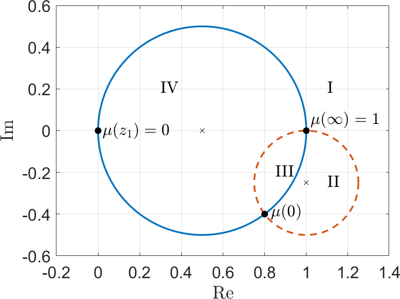
Figure 1: Images under $\mu$ of the real and imaginary axis (solid and dashed circles, respectively) and of the four quadrants; see Remark 4.2 and the proof of Theorem 4.1.

Remark 4.2.

In the proof of Theorem 4.1, we additionally have $\operatorname{Re}(\lambda)\geq 0$. Hence $\sigma$ is located in the image of the (closed) fourth quadrant under $\mu$ in (4.9). To determine this image, note that $\mu$ maps the imaginary axis onto the circle

$$\mathcal{C}_{\beta}=\{z\in\mathbb{C}:\lvert z-(1-{\operatorname{i}}(\beta/2))\rvert=\lvert\beta\rvert/2\},$$ (4.12)

which intersects $\mu(\mathbb{R})=\mathcal{C}$ orthogonally in $\mu(0)$ and $\mu(\infty)=1$. Considering the orientations shows that $\mu$ maps the right half-plane onto the exterior of $\mathcal{C}_{\beta}$; see Figure 1. Thus the spectrum satisfies

$$\sigma(AM^{-1})\subseteq\{z\in\mathbb{C}:\lvert z-1/2\rvert\leq 1/2\}\setminus\{z\in\mathbb{C}:\lvert z-(1-{\operatorname{i}}(\beta/2))\rvert<\lvert\beta\rvert/2\}.$$ (4.13)

In case of Dirichlet boundary conditions, the eigenvalues of $AM^{-1}$ lie on the arc of the circle $\mathcal{C}$ from $\mu(0)$ to $\mu(\infty)=1$ that contains the origin.

This observation further tightens the inclusion set of $\sigma(AM^{-1})$, also in the case of a deterministic wavenumber. This tighter inclusion set is already visible in [8, Fig. 1, Fig. 2] and [9, Fig. 2.1] but we are not aware of a proof in the literature.

5 Mean value preconditioner

We consider the discretization from Section 3.1. Let $S(\xi)\in\mathbb{K}^{n,n}$ be the coefficient matrix of a linear system resulting from a spatial discretization of the Helmholtz equation (2.1) including boundary conditions and wavenumber $k(x,\xi)$. We assume that $S(\xi)$ is non-singular for almost all realizations $\xi\in\Xi$. Let $\bar{\xi}\in\Xi$ be the expected value of the multidimensional random variable $\xi$. It holds that

$$S(\xi)=S(\bar{\xi})+(S(\xi)-S(\bar{\xi}))\eqcolon S(\bar{\xi})+\Delta S(\xi).$$

The stochastic Galerkin method applied to $S(\xi)$ yields a matrix $A\in\mathbb{K}^{(m+1)n,(m+1)n}$ as shown in Section 3.1. Furthermore, we define the constant matrix

$$\bar{A}=I_{m+1}\otimes S(\bar{\xi}).$$ (5.1)

This matrix allows for the construction

$$A=\bar{A}+(A-\bar{A})\eqcolon\bar{A}+\Delta A.$$ (5.2)

We employ the Frobenius matrix norm $\|\cdot\|_{\rm F}$ in the following.

Theorem 5.1.

Using the Frobenius norm, it holds that

$$\|\bar{A}^{-1}A-I_{(m+1)n}\|_{\rm F}\leq C_{m}\,\|S(\bar{\xi})^{-1}\|_{\rm F}\,\big{\|}\|\Delta S(\xi)\|_{\rm F}\big{\|}_{\mathcal{L}^{2}(\Xi,\rho)}$$ (5.3)

with the constants

$$C_{m}=\sqrt{m+1}\,\bigg{(}\sum_{i,j=0}^{m}\|\phi_{i}(\xi)\phi_{j}(\xi)\|_{\mathcal{L}^{2}(\Xi,\rho)}^{2}\bigg{)}^{\frac{1}{2}}$$

provided that the $\mathcal{L}^{2}$-norm of the matrix norm is finite.

Proof.

The definition (5.2) directly yields

$$\bar{A}^{-1}A-I_{(m+1)n}=I_{(m+1)n}+\bar{A}^{-1}\Delta A-I_{(m+1)n}=\bar{A}^{-1}\Delta A.$$

We obtain $\|\bar{A}^{-1}\Delta A\|_{\rm F}\leq\|\bar{A}^{-1}\|_{\rm F}\,\|\Delta A\|_{\rm F}$. The properties of the Kronecker product and (5.1) imply $\|\bar{A}^{-1}\|_{\rm F}^{2}=(m+1)\|S(\bar{\xi})^{-1}\|_{\rm F}^{2}$. We estimate $\lVert\Delta A\rVert_{\rm F}$ using the Cauchy-Schwarz inequality with respect to the inner product (2.5)

$$\|\Delta A\|_{\rm F}^{2} =\sum_{i,j=0}^{m}\sum_{\mu,\nu=1}^{n}\left|\langle\phi_{i}(\xi)\phi_{j}(\xi),\Delta S_{\mu,\nu}(\xi)\rangle\right|^{2}$$

$$\leq\sum_{i,j=0}^{m}\sum_{\mu,\nu=1}^{n}\|\phi_{i}(\xi)\phi_{j}(\xi)\|_{\mathcal{L}^{2}(\Xi,\rho)}^{2}\,\|\Delta S_{\mu,\nu}(\xi)\|_{\mathcal{L}^{2}(\Xi,\rho)}^{2}$$

$$=\bigg{(}\sum_{i,j=0}^{m}\|\phi_{i}(\xi)\phi_{j}(\xi)\|_{\mathcal{L}^{2}(\Xi,\rho)}^{2}\bigg{)}\,\big{\|}\|\Delta S(\xi)\|_{\rm F}\big{\|}_{\mathcal{L}^{2}(\Xi,\rho)}^{2}.$$

In the last step, we used that the square of an $\mathcal{L}^{2}$-norm is an integral and thus summation (with respect to $\mu,\nu$) and integration can be interchanged. Applying the square root to the above estimate yields the statement (5.3). ∎

Remark 5.2.

Rough estimates are used in the proof of Theorem 5.1. Thus the true matrix norms of $\bar{A}^{-1}A-I_{(m+1)n}$ are often much smaller than the upper bounds in (5.3).

Remark 5.3.

If the random variable $\Delta S(\xi)$ is essentially bounded, then it follows that

$$\big{\|}\|\Delta S(\xi)\|_{\rm F}\big{\|}_{\mathcal{L}^{2}(\Xi,\rho)}\leq\sup_{\xi\in\Xi\backslash\Upsilon}\|\Delta S(\xi)\|_{\rm F}<\infty$$

with a set $\Upsilon\subseteq\Xi$ of measure zero due to the normalization $\|1\|_{\mathcal{L}^{2}(\Xi,\rho)}=1$.

Remark 5.4.

The bound of Theorem 5.1 also holds true for the Frobenius norm of $A\bar{A}^{-1}-I_{(m+1)n}$.

Theorem 5.1 together with Remark 5.2 demonstrate that the matrix $\bar{A}$ is a good preconditioner for solving linear systems with coefficient matrix $A$. In this context, $\bar{A}$ is called the mean value preconditioner, as in [29] for the multi-element method. When $\bar{A}$ is used as a preconditioner (left-hand or right-hand), linear systems with coefficient matrix $\bar{A}$ have to be solved. The matrix $\bar{A}$ from (5.1) is block-diagonal with $m+1$ identical blocks in this application. Thus just a single $LU$-decomposition of the matrix $S(\bar{\xi})$ is required. Many linear systems with different right-hand sides are solved using this $LU$-decomposition in an iterative method like GMRES, for example.

Theorem 5.5.

Let $S(\xi)=S_{0}+\theta T(\xi)$ with a non-singular constant matrix $S_{0}$, a matrix $T=\begin{bmatrix}t_{\mu,\nu}\end{bmatrix}_{\mu,\nu}$ depending on a random variable $\xi$ with components $t_{\mu,\nu}\in\mathcal{L}^{2}(\Xi,\rho)$ and a real parameter $\theta>0$. Using $A_{0}=I_{m+1}\otimes S_{0}$, the Frobenius norm exhibits the asymptotic behavior

$$\|A_{0}^{-1}A-I_{(m+1)n}\|_{\rm F}=O(\theta).$$ (5.4)

Proof.

Since the entries of $T(\xi)$ are assumed to be square-integrable, also the expected values are finite. Let $\bar{T}$ be the constant matrix containing the expected values of $T(\xi)$. We apply the decomposition

$$S(\xi)=(S_{0}+\theta\bar{T})+\theta(T(\xi)-\bar{T}).$$

The matrix $S_{0}+\theta\bar{T}$ is non-singular for sufficiently small $\theta$. Moreover, we obtain the relation $(S_{0}+\theta\bar{T})^{-1}=S_{0}^{-1}+O(\theta)$. Theorem 5.1 yields

$$\|\bar{A}^{-1}A-I_{(m+1)n}\|_{\rm F}\leq C_{m}\,\|(S_{0}+\theta\bar{T})^{-1}\|_{\rm F}\,\big{\|}\|\theta(T-\bar{T})\|_{\rm F}\big{\|}_{\mathcal{L}^{2}(\Xi,\rho)}$$

with $\bar{A}=I_{m+1}\otimes(S_{0}+\theta\bar{T})$. It holds that $\bar{A}=A_{0}+O(\theta)$ and thus $\bar{A}^{-1}=A_{0}^{-1}+O(\theta)$. We conclude

$$\|{A}_{0}^{-1}A-I_{(m+1)n}\|_{\rm F}\leq\left(C_{m}\,\left(\|S_{0}^{-1}\|_{\rm F}+O(\theta)\right)\,\theta\,\big{\|}\|T-\bar{T}\|_{\rm F}\big{\|}_{\mathcal{L}^{2}(\Xi,\rho)}\right)+O(\theta)=O(\theta),$$

which confirms (5.4). ∎

An important case of Theorem 5.5 is $\bar{T}=0$, i.e., these expected values are zero. Then $A_{0}=\bar{A}$ is the mean value preconditioner.

Corollary 5.6.

Under the assumptions of Theorem 5.1, the Frobenius norm satisfies the estimate

$$\|\bar{A}^{-1}A-I_{(m+1)n}\|_{\rm F}<1$$ (5.5)

for all sufficiently small $\Delta S$.

Likewise, the Frobenius norm using $A_{0}$ instead of $\bar{A}$ is smaller than one if the parameter $\theta$ is sufficiently small in the context of Theorem 5.5.

A stationary iterative scheme for solving a linear system $Ax=b$ reads as

$$Bx^{(i+1)}=b-(A-B)x^{(i)}\qquad\mbox{for}\;i=0,1,2,\ldots$$ (5.6)

with a non-singular matrix $B$ which should approximate $A$, see [26, p. 621]. In each iteration step, we have to solve a linear system with coefficient matrix $B$. The property (5.5) is sufficient for the global convergence of the iteration (5.6) using $B=\bar{A}$. The computational cost of an iteration step is much less than the steps in GMRES using $\bar{A}$ as preconditioner, because the construction of Krylov subspaces is avoided. In practice, we do not know if $\Delta S$ is sufficiently small such that the bound (5.5) is guaranteed. Nevertheless, it is worth to try this stationary iteration, as we will observe in Section 7.

6 Numerical experiments in 1D

Our model problem in one space dimension is the stochastic Helmholtz equation (3.1) on $Q=]0,1[$ with absorbing boundary conditions. The right-hand side is the point source $f(x)=\delta(x-\frac{1}{2})$, similarly to, e.g., [9, 18, 25, 27], where the right-hand side is a (possibly scaled) point source. We consider a random wavenumber $k(x,\xi)=k(\xi)$ constant in space, which is uniformly distributed in some interval $[k_{\min},k_{\max}]$ with $0<k_{\min}<k_{\max}$. Equivalently, we define

$$k(\xi)=(1+\theta\xi)\overline{k}$$ (6.1)

with a random variable $\xi$ that is uniformly distributed in $[-1,1]$, a mean value $\overline{k}$, and a real parameter $\theta\in]0,1[$. It follows that $k_{\min}=(1-\theta)\overline{k}$ and $k_{\max}=(1+\theta)\overline{k}$.

In our numerical experiments in one and two spatial dimensions, we compute the mesh-size $h=\frac{1}{q+1}$ in the FD discretization by

lev = max(ceil(log2((15*maxk)/(2*pi))), 1);
q = 2^lev - 1;

where maxk is the maximal value of the wavenumber. Then the relation $\frac{2\pi}{kh}\approx\text{constant}$, advocated in [16, Sect. 4.4.1], is satisfied. Indeed, the estimate $x\leq\lceil x\rceil\leq x+1$ for $x\in\mathbb{R}$ implies $\frac{15k}{2\pi}\leq q+1\leq 2\frac{15k}{2\pi}$ for large $k$. In particular, $q$ grows linearly with $k$ and thus the size of the matrices $S(\xi)$ and $A$ (see Section A) grows with $k$; see, e.g., Figure 3. Our choice for $q$ can be adapted for a future use of a multigrid method (as in [9]).

Discretizing the model problem yields a linear algebraic system

$$Ax=b$$ (6.2)

as given in Theorem A.2. This one-dimensional problem can be solved by a direct method, since the computational work is not too large. Nevertheless we also consider its solution with the GMRES method [24] and investigate the application of CSL and mean value preconditioners introduced in Sections 4 and 5, respectively.

By Theorem A.2, the matrix $A$ has the form

$$A=I_{m+1}\otimes T-{\operatorname{i}}[B_{ij}]-[C_{ij}].$$ (6.3)

If needed, we write $A_{\theta}$ to indicate the dependence of $A$ on $\theta$, and in particular $A_{0}$ for $\theta=0$, which corresponds to the mean value preconditioner. Since the wavenumber in (6.1) is constant in space, the matrices $[B_{ij}]$ and $[C_{ij}]$ simplify to

$$[B_{ij}] =\begin{bmatrix}\langle k(\xi)\phi_{j}(\xi),\phi_{i}(\xi)\rangle\end{bmatrix}_{ij}\otimes D_{1}, D_{1} =\frac{1}{h}\operatorname{diag}(1,0,\ldots,0,1),$$ (6.4)

$$[C_{ij}] =\begin{bmatrix}\langle k(\xi)^{2}\phi_{j}(\xi),\phi_{i}(\xi)\rangle\end{bmatrix}_{ij}\otimes D_{2}, D_{2} =\operatorname{diag}\Bigl{(}\frac{1}{2},1,\ldots,1,\frac{1}{2}\Bigr{)},$$ (6.5)

see Lemma A.4, and, by Lemma A.3,

$$B_{ij}=0\quad\text{for }\lvert i-j\rvert>1,\quad C_{ij}=0\quad\text{for }\lvert i-j\rvert>2.$$ (6.6)

In other words, the matrices $\begin{bmatrix}\langle k(\xi)\phi_{j}(\xi),\phi_{i}(\xi)\rangle\end{bmatrix}_{ij}$ and $\begin{bmatrix}\langle k(\xi)^{2}\phi_{j}(\xi),\phi_{i}(\xi)\rangle\end{bmatrix}_{ij}$ are tridiagonal and pentadiagonal, respectively, due to the orthogonality properties of the polynomials.

Remark 6.1.

In the deterministic case $k(\xi)=\overline{k}$ in (6.1), i.e., $\theta=0$, the matrices $[B_{ij}]=\overline{k}I_{m+1}\otimes D_{1}$ and $[C_{ij}]=\overline{k}^{2}I_{m+1}\otimes D_{2}$ are diagonal, and

$$A_{0}=I_{m+1}\otimes(T-{\operatorname{i}}\overline{k}D_{1}-\overline{k}^{2}D_{2})=I_{m+1}\otimes S(0)$$ (6.7)

with $S(\xi)$ from Theorem A.2. This shows that $A_{0}$ is block-diagonal with $m+1$ identical diagonal blocks. The latter are the FD-discretization of the deterministic Helmholtz equation with wavenumber $\overline{k}$ (associated to $\xi=0$).

If not specified otherwise, we use $m=3$ in the stochastic Galerkin method and $\theta=0.1$ in (6.1). Finally, we also consider the shifted Helmholtz equation (4.1) with shift $\beta=\frac{1}{2}$ and denote the CSL preconditioner by $M=M(\frac{1}{2})$, see (4.2). As for $A$, we write $M_{\theta}$ if we wish to emphasize the dependence on $\theta$.

The numerical experiments have been performed in the software package MATLAB R2020b on an i7-7500U @ 2.70GHz CPU with 16 GB RAM.

6.1 Spectra

By Theorem 4.1, the eigenvalues of the CSL preconditioned matrix $AM^{-1}$ lie in the closed disk (4.3). This is illustrated in the left panel of Figure 2, which displays the spectra of $AM^{-1}$ (with $\theta=0.1$) and $A_{0}M_{0}^{-1}$ (i.e., with $\theta=0$). Each eigenvalue of $A_{0}M_{0}^{-1}$ is $(m+1)$-fold, since $A_{0}=I_{m+1}\otimes S(0)$ is block-diagonal with identical diagonal blocks, see Remark 6.1, and similarly for $M_{0}$. For $\theta\neq 0$, the matrix $AM^{-1}$ is not block-diagonal, and $AM^{-1}$ has clusters of $m+1$ eigenvalues close to each $(m+1)$-fold eigenvalue of $A_{0}M_{0}^{-1}$. This can be observed in the figure with $m+1=4$. The right panel in Figure 2 displays the spectrum of $AA_{0}^{-1}$ for the mean value preconditioner. The eigenvalues are clustered at $1$, which suggests a fast convergence of GMRES. If the eigenvalues satisfy $\lvert\lambda-1\rvert<1$ then the stationary method (5.6) with $B=A_{0}$ converges.

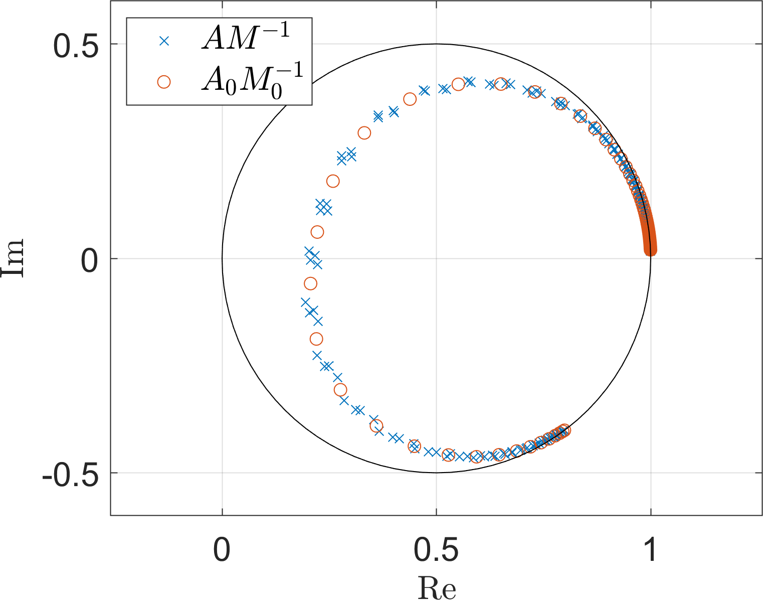
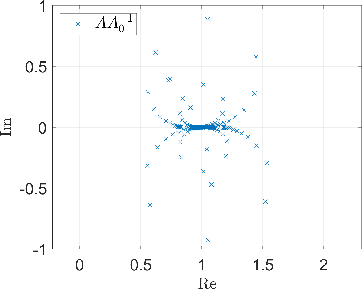
Figure 2: Left: Spectrum of $AM^{-1}$ for $\overline{k}=50$, $m=3$, $\theta=0.1$ (crosses) and $\theta=0$ (circles). The large solid circle illustrates (4.4). Right: Spectrum of $AA_{0}^{-1}$.

6.2 Condition numbers

Figure 3 displays the 2-norm condition numbers of $A$, $M$, $AM^{-1}$, $A_{0}$ and $AA_{0}^{-1}$ as functions of $\overline{k}$ (with $\theta=0.1$). Clearly, the condition numbers of $M$ and $AM^{-1}$ are much smaller than the condition number of $A$, which is beneficial when solving the preconditioned linear system $AM^{-1}y=b$, $Mx=y$ with the CSL preconditioner. In this example, $\kappa_{2}(M)\leq 205$ for all $\overline{k}$, which is very moderate, and $\kappa_{2}(AM^{-1})$ grows linearly in $\overline{k}$ from $2.6485$ when $\overline{k}=10$ to only $36.5190$ when $\overline{k}=200$. In contrast, $\kappa_{2}(A)$ is roughly $50$ to $160$ times larger than $\kappa_{2}(AM^{-1})$. The observed spikes of $\kappa_{2}(A)$ occur when more discretization points are used which leads to a larger size of $A$, compare the curve of size(A). The condition number of the mean value preconditioned matrix $AA_{0}^{-1}$ is also moderate, growing from $2$ to $141$, which is beneficial for solving the preconditioned linear system, while $\kappa_{2}(A_{0})$ is of the order of $\kappa_{2}(A)$.

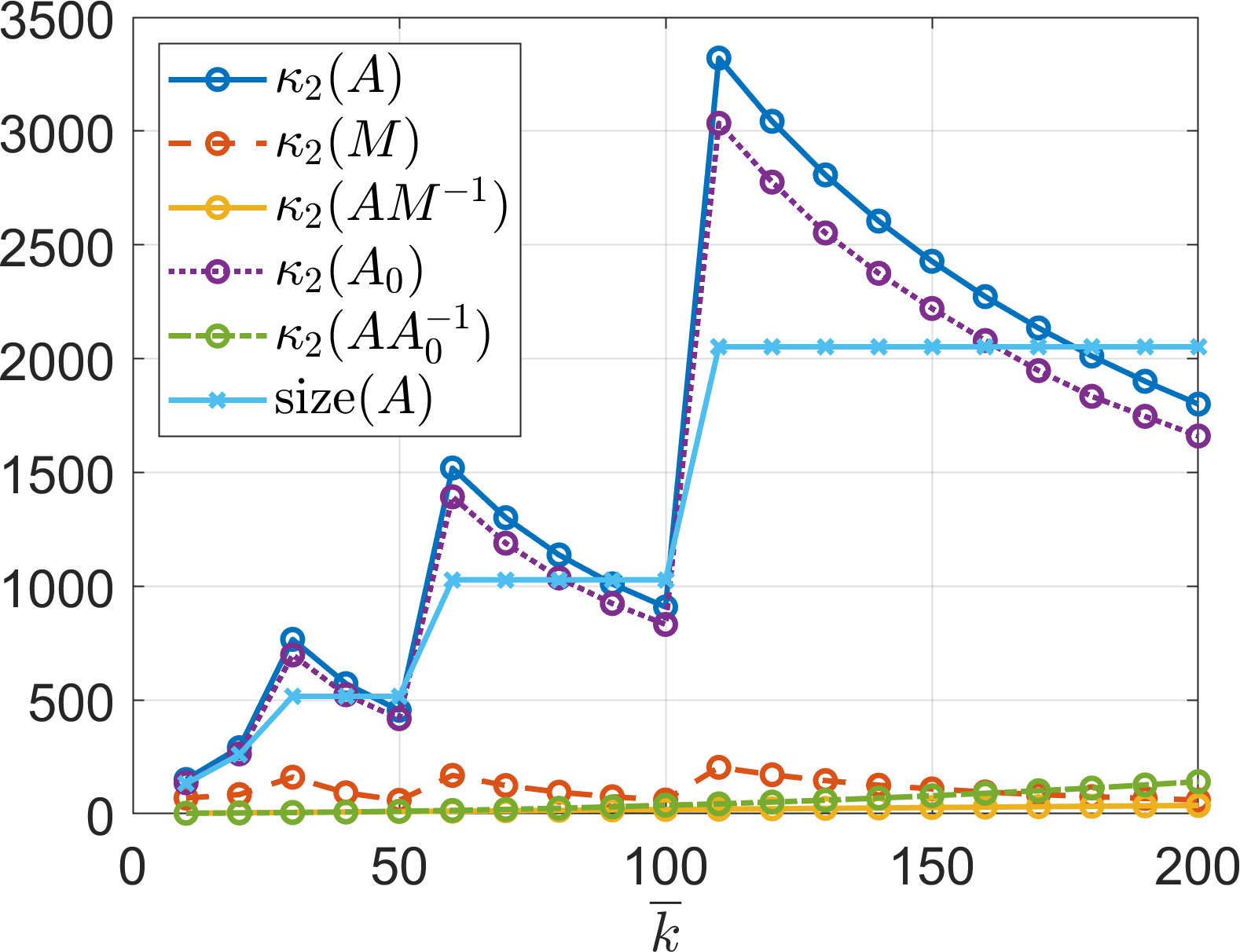
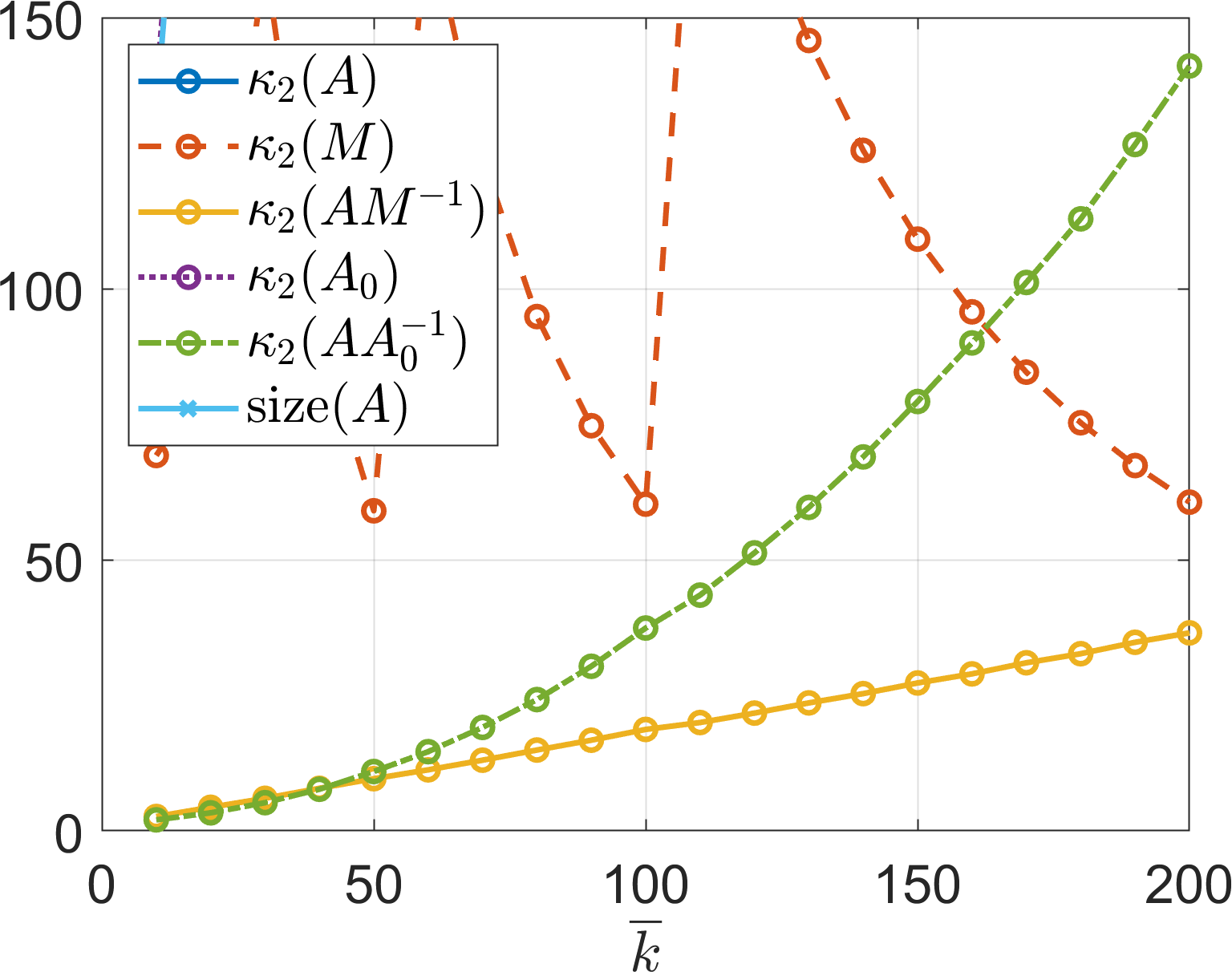
Figure 3: $2$-norm condition numbers as functions of $\overline{k}$ (left) and zoom-in (right).

6.3 GMRES

We solve the unpreconditioned system (6.2) and the right and left preconditioned systems

$$AM^{-1}y=b,\quad x=M^{-1}y,\qquad\text{and}\qquad M^{-1}Ax=M^{-1}b$$ (6.8)

with full GMRES (no restarts) and tolerance tol=1e-12, using MATLAB’s built-in gmres command. The residual in the $i$th step is $r^{(i)}=b-Ax^{(i)}$ for unpreconditioned and right preconditioned GMRES, and $M^{-1}r^{(i)}$ for left preconditioned GMRES. In particular, the stopping criterion for left and right preconditioning is in general different. We will consider the following three preconditioners:

1. the CSL preconditioner $M$,

2. the mean value preconditioner $A_{0}$,

3. the mean value CSL preconditioner $M_{0}$.

In preconditioned GMRES, we need to solve linear systems with the preconditioner, for which we use an $LU$-decomposition. In one spatial dimension, this is not competitive with the direct solution (see the end of Section 6.3), but in two spatial dimension the block structure of the preconditioners $A_{0}$ and $M_{0}$ leads to a competitive method. In MATLAB, the $LU$-decomposition of the sparse matrix $M$ calls the associated routine from UMFPACK; see [4]. The decomposition has the form

$$PMQ=LU$$ (6.9)

with a lower triangular matrix $L$, upper triangular matrix $U$, and two permutation matrices $P,Q$. In our implementation, we use

[L, U, p, q] = lu(M, ’vector’);
qt = []; qt(q) = 1:numel(q);

where, instead of the matrices $P,Q$, only vectors $p,q$ representing the permutations are stored, and where the vector qt describes the inverse mapping of the permutation defined by q. Then, we implement $M^{-1}x$ by

x = U\(L\x(p,:));
x = x(qt,:);

By Remark 6.1, $A_{0}=I_{m+1}\otimes S(0)$ is block-diagonal with equal diagonal blocks so that, for fixed $\overline{k}$, only a single $LU$-decomposition of $S(0)\in\mathbb{K}^{n,n}$ is necessary to compute $A_{0}^{-1}x$ for any vector $x\in\mathbb{K}^{(m+1)n}$. In our implementation, we partition and reshape $x$ so that only one linear system with $S(0)$ is solved:

x = reshape(x, [n, m+1]);
x = U\(L\x(p,:));
x = x(qt,:);
x = reshape(x, [], 1);

The preconditioner $M_{0}$ is implemented in the same way.

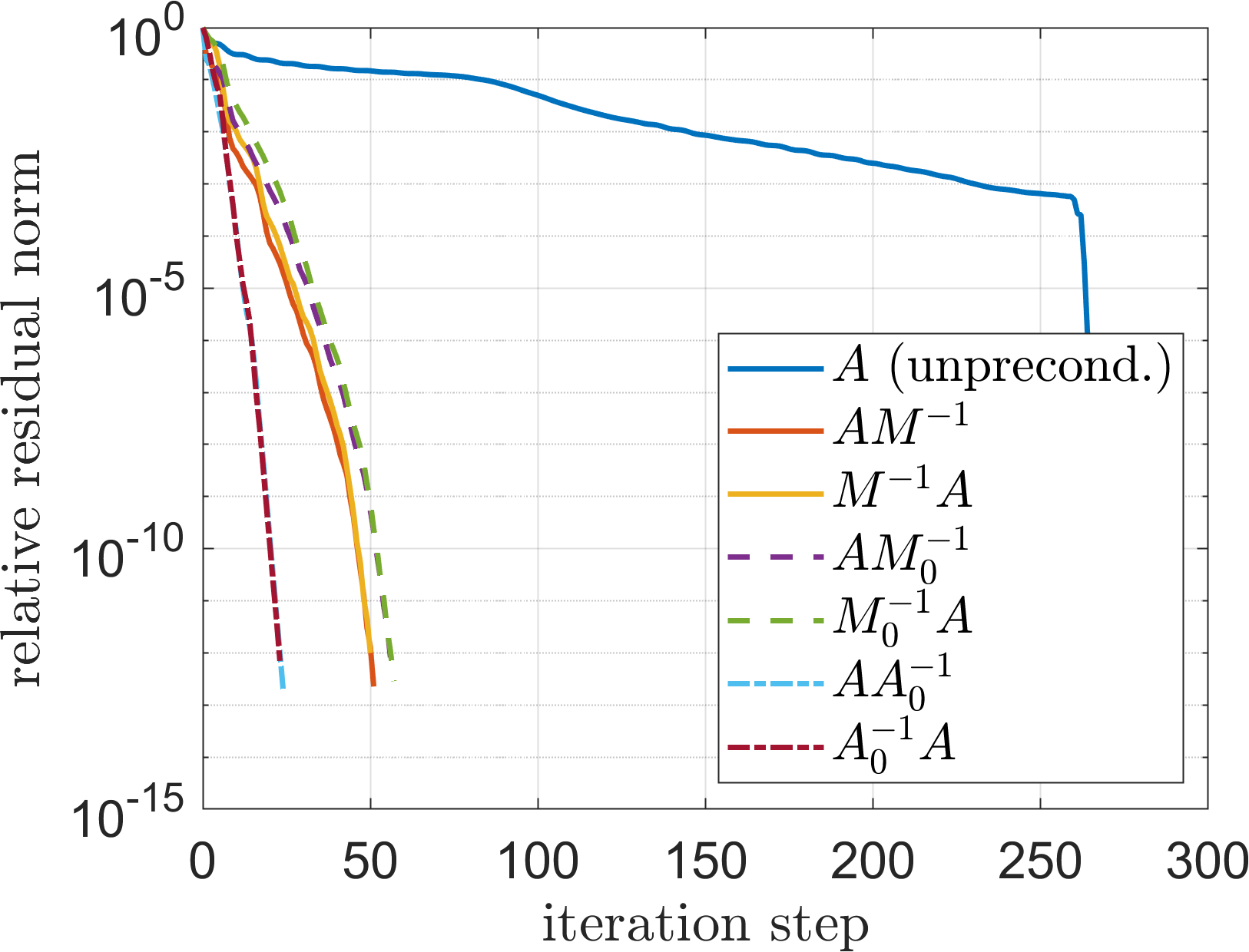
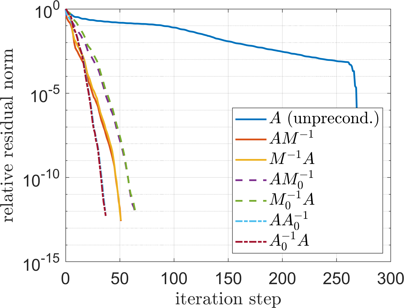
Figure 4: Relative residual norms when solving (6.2) with GMRES with various preconditioners, $m=3$, $\overline{k}=50$, and $\theta=0.1$ (left) or $\theta=0.2$ (right).

	$\theta=0.1$		$\theta=0.2$
preconditioner	left	right	left	right
unpreconditioned	$0.5509$		$0.5409$
$M^{-1}$	$0.0291$	$0.0320$	$0.0298$	$0.0322$
$M_{0}^{-1}$	$0.0316$	$0.0339$	$0.0395$	$0.0401$
$A_{0}^{-1}$	$0.0148$	$0.0148$	$0.0211$	$0.0198$

Table 1: Time in seconds (s) for solving (6.2) and (6.8) with GMRES.

In a first experiment, we fix $\overline{k}=50$, $\theta=0.1$ and $m=3$. Solving the unpreconditioned system (6.2) with GMRES suffers from a long delay of convergence; see Figure 4. In contrast, all three preconditioners $M$, $M_{0}$, and $A_{0}$ lead to a significant decrease in the number of iteration steps from about $250$ to $50$ for $M$ and $M_{0}$ (factor $5$), and to about $25$ for $A_{0}$ (factor $10$); see Figure 4 (left panel). The computation times with the preconditioners $M$ and $M_{0}$ reduce to about $6\%$ of the computation time of unpreconditioned GMRES, while for $A_{0}$ it reduces to about $3\%$; see Table 1. The computation times for the preconditioned systems include the computation of the $LU$-decomposition (of $M$ or of a diagonal block for $A_{0}$ or $M_{0}$). The differences between computed solutions are very small: $\lVert x-x^{\prime}\rVert_{\infty}\leq 1.7\cdot 10^{-14}$ (and typically of order $10^{-15}$), where x=A\b is the direct solution and $x^{\prime}$ is a solution computed with GMRES (unpreconditioned or with one of the preconditioners). Left and right preconditioning lead to very similar relative residual norms and timings for each preconditioner. A heuristic explanation why $A_{0}$ performs better than $M$ and $M_{0}$, is that $A$ is closer to $A_{0}$ than to $M$ or $M_{0}$. Indeed, we have $\lVert A-A_{0}\rVert_{\infty}<\lVert A-M\rVert_{\infty}<\lVert A-M_{0}\rVert_{\infty}$ in this example. Repeating this experiment with $\theta=0.2$ leads to very similar results, see Figure 4 and Table 1, so we focus on $\theta=0.1$.

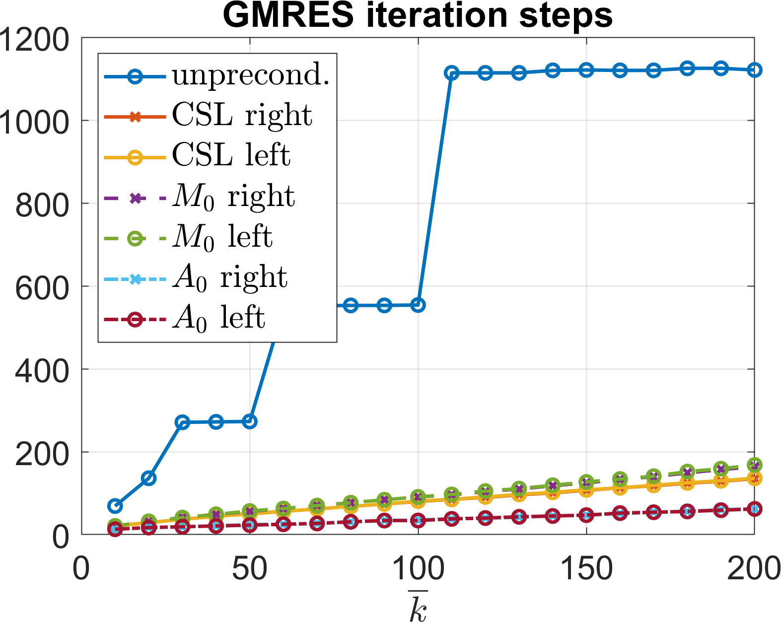
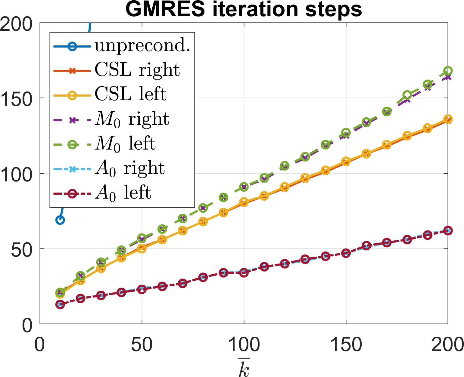
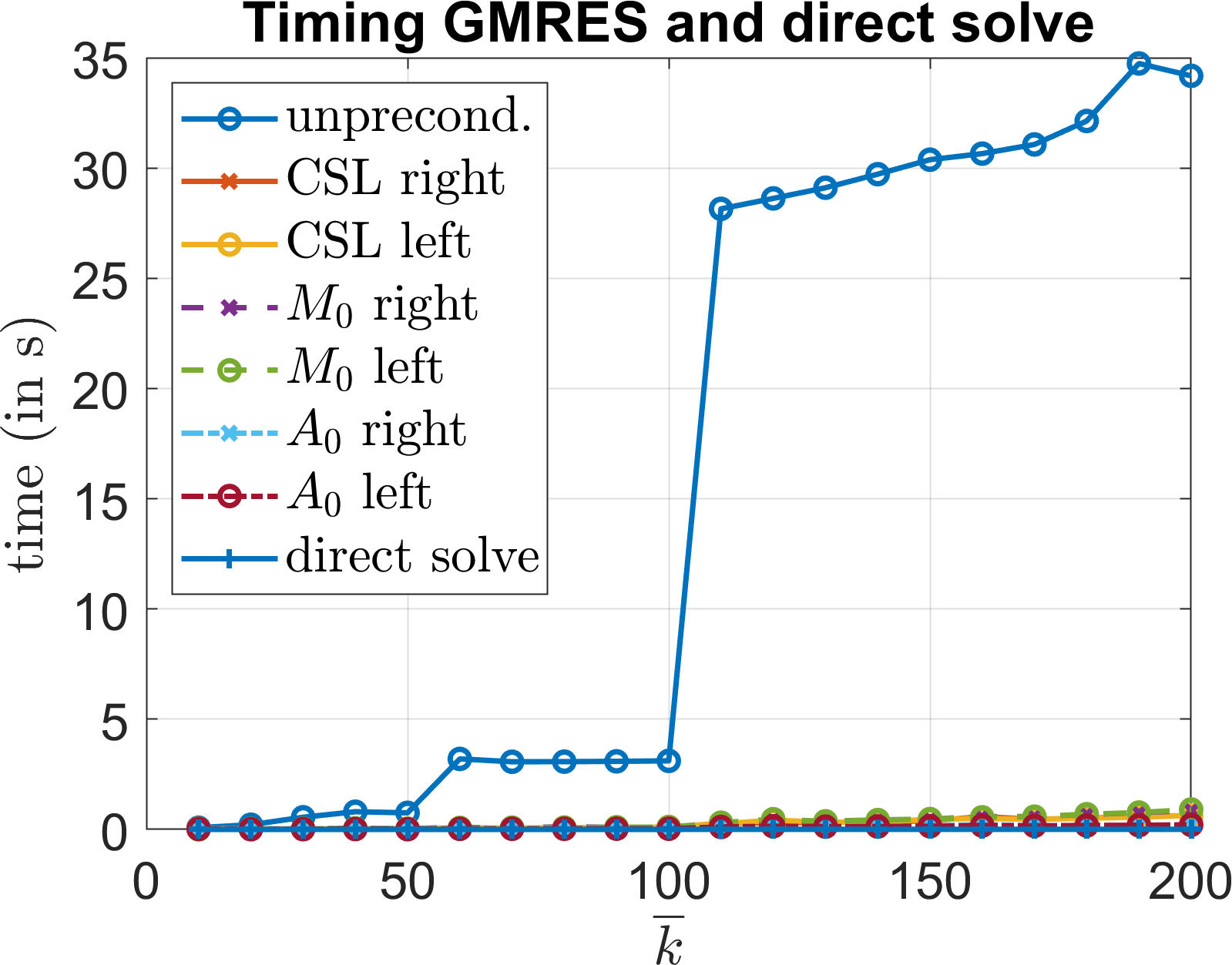
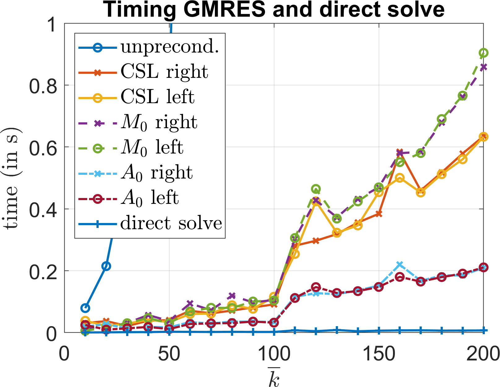
Figure 5: Number of GMRES iteration steps (top) and computation time in seconds (bottom) as functions of $\overline{k}$ for different left and right preconditioners with fixed $\theta=0.1$ and $m=3$. The right panels are zoom-ins.

In a second experiment, we let $\overline{k}$ vary while $\theta=0.1$ and $m=3$ are fixed. Figure 5 displays the number of GMRES iteration steps (top) and the computation time (bottom) as functions of $\overline{k}$. For small $\overline{k}\in[10,50]$, the difference between unpreconditioned and preconditioned GMRES is not so pronounced, since the linear systems are rather small. For $60\leq\overline{k}\leq 200$, the three preconditioners significantly reduce the number of iteration steps and the computation time compared to unpreconditioned GMRES. The number of iteration steps is reduced to 8–15% of the number of iteration steps in unpreconditioned GMRES when using $M$, to 9–16% when using $M_{0}$ and to only 3–6% when using $A_{0}$ as preconditioner. GMRES preconditioned with $M$ or $M_{0}$ needs only 1–4% of the computation of unpreconditioned GMRES, and the computation time of GMRES preconditioned with $A_{0}$ is reduced to 0.5–1.1% of the computation time of unpreconditoned GMRES. The mean value preconditioner $A_{0}$ leads to the smallest number of GMRES iteration steps and computation time, which is likely due to the fact that $A$ is closer to $A_{0}$ than to $M$ or $M_{0}$. Note, however, that the condition number of $A_{0}$ (and $A$) is much larger than that of $M$ and $M_{0}$. For $\overline{k}=150$, we have (rounded to the nearest integer) $\kappa_{2}(A)=2428$, $\kappa_{2}(A_{0})=2220$, $\kappa_{2}(M)=109$, $\kappa_{2}(M_{0})=91$; see also Figure 3. Thus, if accuracy is an issue, it is preferable to work with the CSL preconditioners $M$ or $M_{0}$.

Finally, we note that the direct solution A\b with a sparse matrix in MATLAB calls an efficient algorithm from UMFPACK; see [4]. In the above test example, solving the linear system (6.2) by GMRES (with or without preconditioner) is not competitive with this direct solution, as it is much faster; see the bottom right panel in Figure 5.

6.4 Solutions

Figure 6 displays the real and imaginary parts of the computed coefficients $v_{0}$, $v_{1}$, $v_{2}$, $v_{3}$ in the Galerkin approximation for $\overline{k}=50$ and $\theta=0.1$ in (6.1). We recognize an effect of the point source at $x=\frac{1}{2}$ in the real part of $v_{0}$.

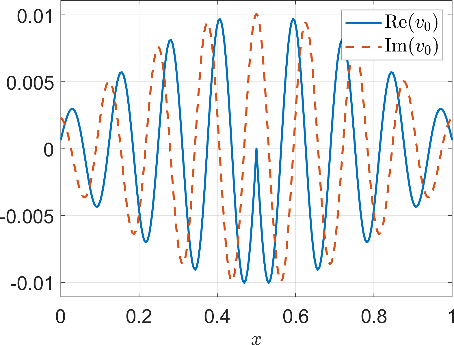
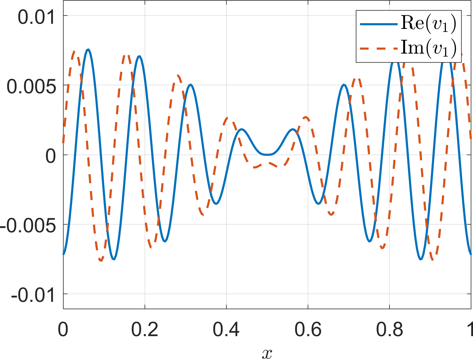
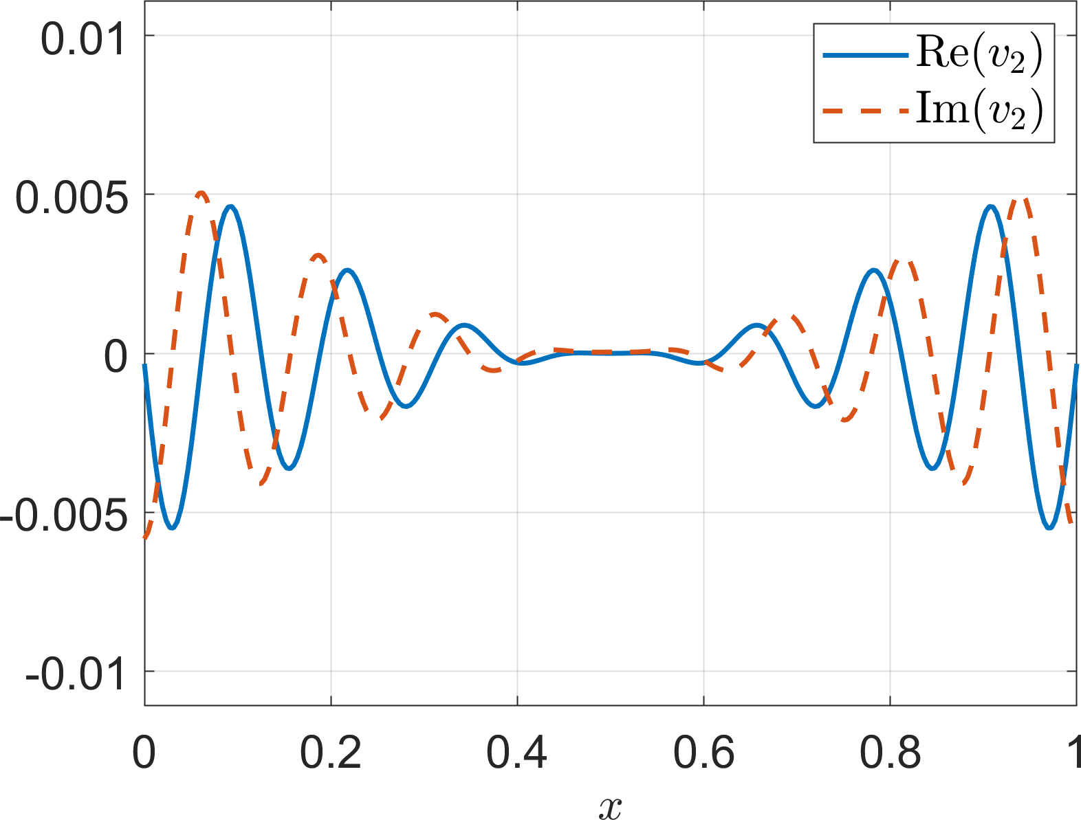
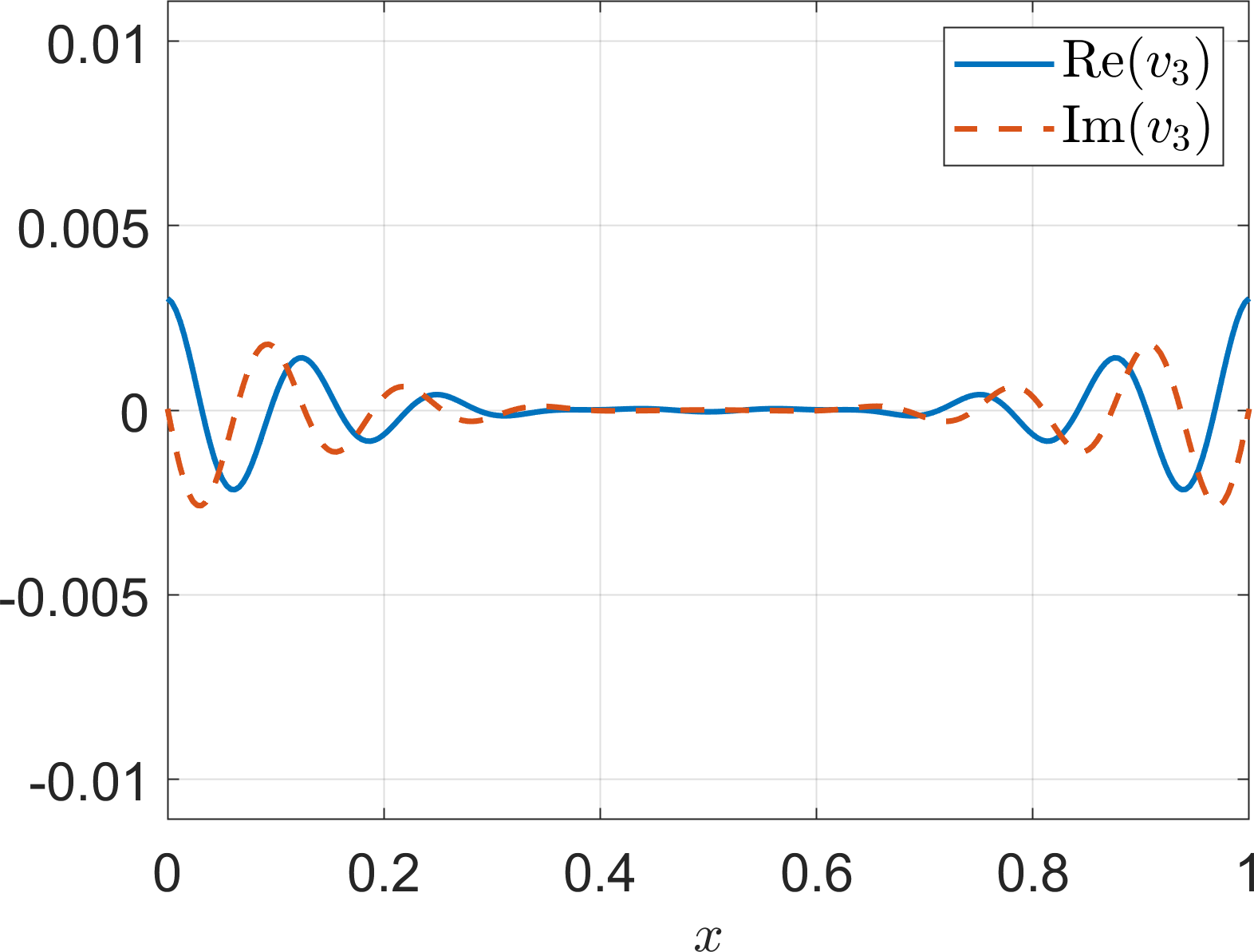
Figure 6: Plots of the coefficients $v_{0},v_{1},v_{2},v_{3}$ for $\overline{k}=50$ and $\theta=0.1$.

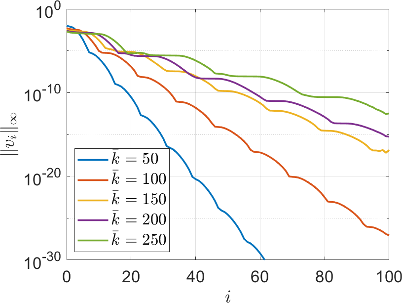
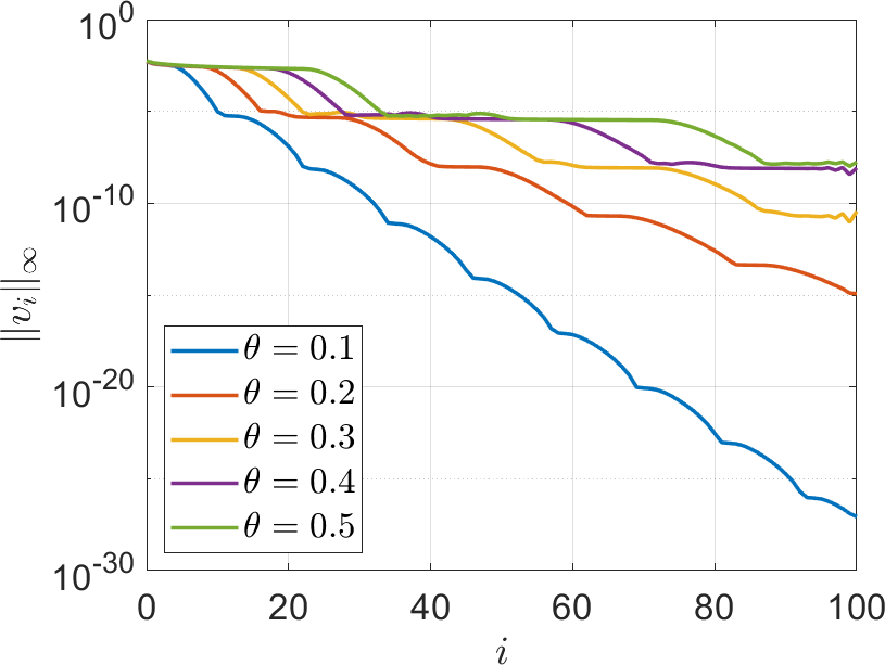
Figure 7: Maximum-norms $\lVert v_{i}\rVert_{\infty}$ as a function of $i=\deg(\phi_{i})$. Left: For fixed $\theta=0.1$ and different values of $\overline{k}$. Right: For fixed $\overline{k}=100$ and different values of $\theta$.

We compute the solution for total polynomial degree $m=100$. Figure 7 shows $\lVert v_{i}\rVert_{\infty}$ as a function of the polynomial degree $i$. In the left panel, $\theta=0.1$ is fixed and $\overline{k}$ varies, while in the right panel $\theta$ varies and $\overline{k}=100$ is fixed. We observe an exponential decay of the coefficients in all cases, which is related to the exponential convergence of the PC expansion (2.7). Larger wavenumbers and larger values of $\theta$ lead to a slower decay of the maximum-norm of the coefficients. The effect of larger $\theta$ on the convergence/decay is more pronounced, compare, for example, the curve for $(\overline{k},\theta)=(150,0.1)$ in the left panel with the curve for $(100,0.5)$ in the right panel.

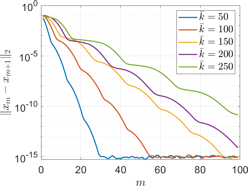
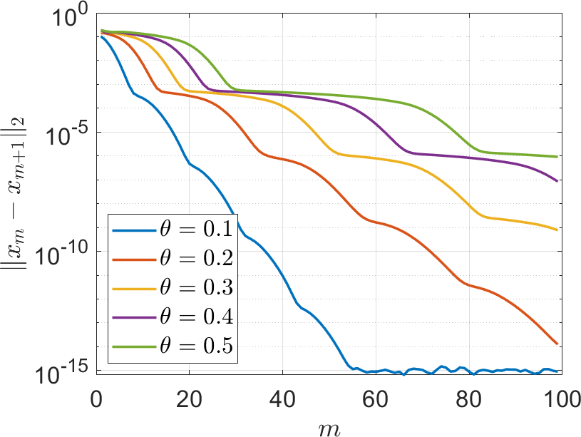
Figure 8: Norms $\lVert x_{m}-x_{m+1}\rVert_{2}$ as a function of the maximal degree $m$ in the stochastic Galerkin method. Left: For fixed $\theta=0.1$ and different values of $\overline{k}$. Right: For fixed $\overline{k}=100$ and different values of $\theta$.

Next, we vary $m$ (the maximal degree of the polynomials in the stochastic Galerkin method) and denote by $x_{m}$ the solution of (6.2), which consists of a discretization of the coefficients $v_{0,m},\ldots,v_{m,m}$ in a Galerkin approximation (3.14) of the solution $u$ of the Helmholtz equation; see also Remark 3.1. The convergence of the stochastic Galerkin method is illustrated by the exponential decay of the norms $\lVert x_{m}-x_{m+1}\rVert_{2}$ in Figure 8.

7 Numerical experiments in 2D

We consider the stochastic Helmholtz equation (3.1) in $Q=]0,1[^{2}$ with absorbing boundary conditions (3.3), the point source $f(x,y)=\delta((x,y)-(\frac{1}{2},\frac{1}{2}))$ as right-hand side, and space-dependent random wavenumber

$$k(x,y,\xi_{1},\xi_{2},\xi_{3})=\begin{cases}(1+\theta\xi_{1})k_{1},&y\leq 0.2+0.1x,\\ (1+\theta\xi_{2})k_{2},&0.2+0.1x<y<0.6-0.2x,\\ (1+\theta\xi_{3})k_{3},&0.6-0.2x\leq y.\end{cases}$$ (7.1)

on the wedge-shaped domain from [18, p. 146]; similar domains have been examined in [6, Sect. 6.3] and [8, Sect. 4.4]. The modeling (7.1) can also be written in the form (2.4) using spatial indicator functions. The random variables $\xi_{1},\xi_{2},\xi_{3}$ are independent and uniformly distributed in $[-1,1]$. The mean value of the wavenumber is

$$\overline{k}(x,y)=\begin{cases}k_{1},&y\leq 0.2+0.1x,\\ k_{2},&0.2+0.1x<y<0.6-0.2x,\\ k_{3},&0.6-0.2x\leq y.\end{cases}$$ (7.2)

We discretize the boundary value problem as described in Section 3.1 and obtain the linear algebraic system $Ax=b$ in Theorem A.6. The number of polynomials in the three random variables $\xi_{1},\xi_{2},\xi_{3}$ with total degree at most $r$ is, see (2.6),

$$m+1=\textstyle\frac{(r+3)!}{r!\,3!}.$$ (7.3)

Table 2 includes the number of basis polynomials for degrees $r=0,1,\ldots,8$.

$r$	n.basis	size of $A$	nnz	time (s)
$0$	$1$	$16641$	$82689$	$0.3264$
$1$	$4$	$66564$	$364038$	$0.6592$
$2$	$10$	$166410$	$993300$	$1.4090$
$3$	$20$	$332820$	$2119728$	$3.3421$
$4$	$35$	$582435$	$3892575$	$10.3049$
$5$	$56$	$931896$	$6461094$	$32.8872$
$6$	$84$	$1397844$	$9974538$	$101.1674$
$7$	$120$	$1996920$	$14582160$	$291.5063$
$8$	$165$	$2745765$	$20433213$	$802.0748$

Table 2: For different total degrees $r$, number of basis polynomials (n.basis), size of the matrix $A$, number of non-zero elements in $A$ (nnz), and time to generate $A$.

Let $k_{1}=30$, $k_{2}=15$, $k_{3}=20$, and $\theta=0.1$. Table 2 shows the size of $A$ and the time (in seconds) for constructing the matrix $A$ for polynomial degrees up to $r=0,1,\ldots,8$ in the stochastic Galerkin method. The computation time when solving $Ax=b$ directly with x=A\b in MATLAB grows exponentially as a function of $r$, see Figure 9 (left panel).

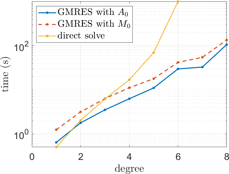
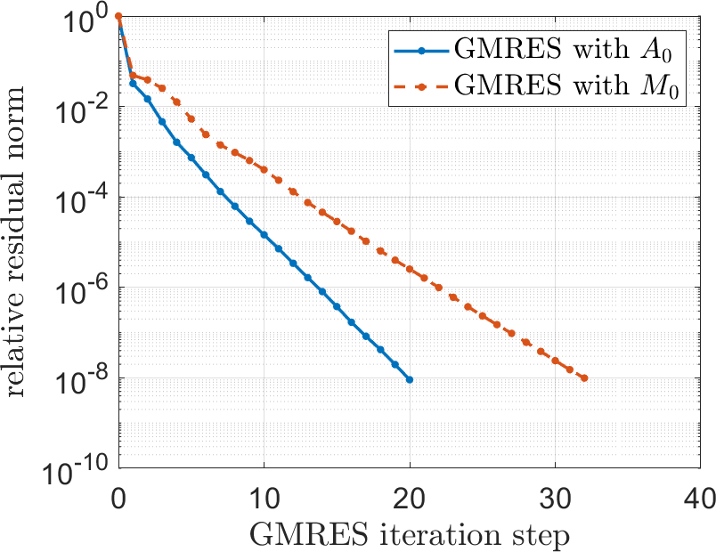
Figure 9: Solving the linear system directly and with GMRES preconditioned by $A_{0}$ and $M_{0}$; see Section 7. Left: Computation time (in seconds) as a function of the polynomial degree $r$ in the stochastic Galerkin method. Right: Relative residual norms in preconditioned GMRES for polynomial degree $r=8$.

Thus we solve the linear algebraic system $Ax=b$ with GMRES using the mean value preconditioner $A_{0}=I_{m+1}\otimes S_{0}$ from (5.1) as right preconditioner, that is, we solve

$$AA_{0}^{-1}y=b,\quad A_{0}x=y.$$ (7.4)

Here $S_{0}$ denotes the FD discretization of the Helmholtz equation with absorbing boundary conditions and deterministic wavenumber (7.2); see Theorem A.6. The solution of linear systems with the preconditioner $A_{0}$ is implemented as described in Section 6.3. We solve (7.4) with full GMRES (no restarts), tol=1e-8 and maxit=200 for polynomial degrees up to $r=1,\ldots,8$ in the stochastic Galerkin method. In contrast to the experiments in 1D in Section 6, preconditioned GMRES is significantly faster than the direct solution with MATLAB’s ‘backslash’ command x=A\b; see Figure 9 (left panel). The computation times for preconditioned GMRES include the computation of the $LU$-decomposition of a diagonal block of $A_{0}$. Furthermore, the relative residual norms in GMRES for polynomial degree $r=8$ are shown in Figure 9 (right panel). The mean value CSL preconditioner $M_{0}$ has a similar block-diagonal structure to $A_{0}$ and performs similarly well; see Figure 9.

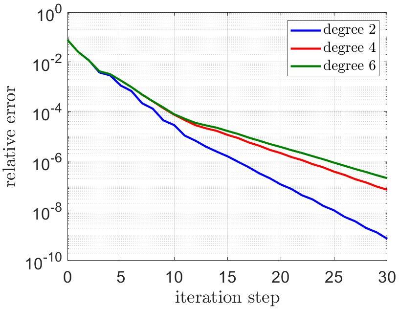
Figure 10: Relative error norms in the stationary iteration (7.5) for different polynomial degrees $r$ in the stochastic Galerkin method.

Alternatively to GMRES or a direct solution of the linear system, we also investigate the stationary iteration (5.6) with $B=A_{0}$, i.e.,

$$A_{0}x^{(i+1)}=b-(A-A_{0})x^{(i)}\quad\text{for }i=0,1,2,\ldots\,.$$ (7.5)

We take the starting vector $x^{(0)}=A_{0}^{-1}b$. Linear systems with the matrix $A_{0}$ are solved as described above. For $\theta=0.1$, this iteration converges. Figure 10 displays the relative error norms in the maximum-norm for polynomial degrees $r=2,4,6$, where we take the direct solution A\b as the ‘exact’ solution. The slower convergence for larger degree $r$ in the stochastic Galerkin method is expected, since the matrix size also grows causing higher condition numbers. For $\theta=0.2$, the stationary iteration diverges. This behavior is in agreement to Theorem 5.5 and Corollary 5.6.

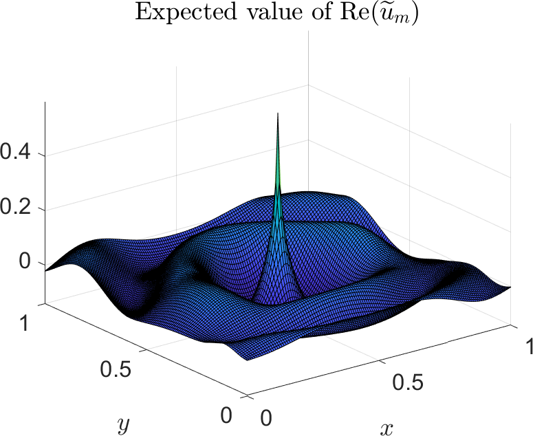
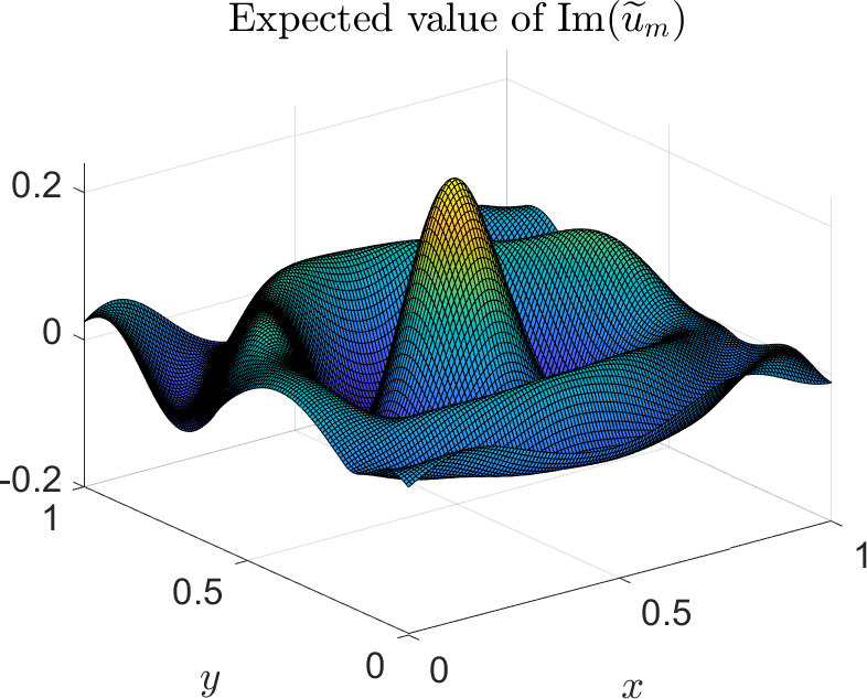
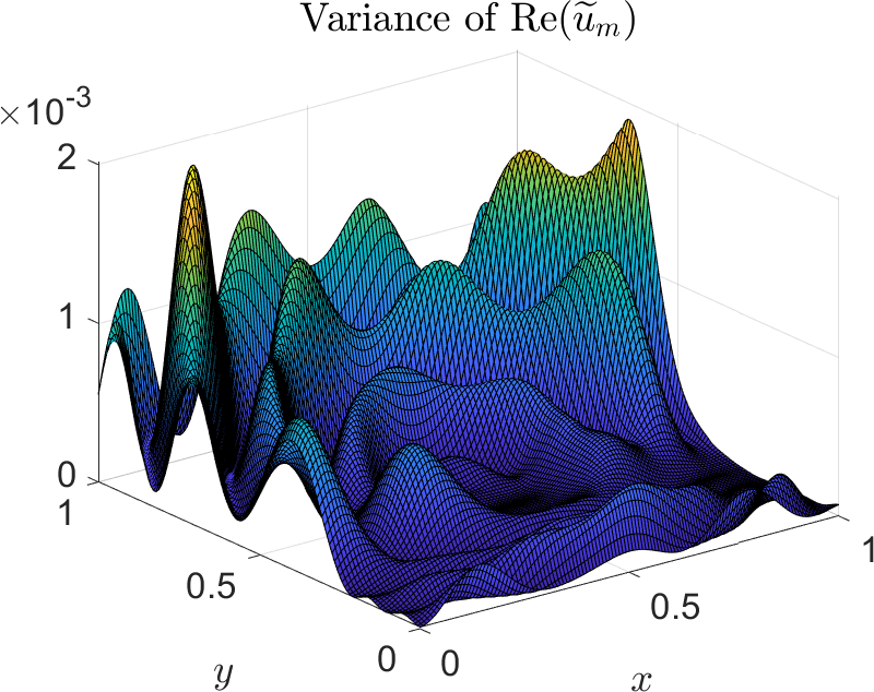
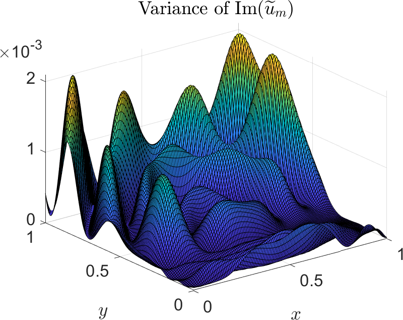
Figure 11: Expected value (top) and variance (bottom) of $\operatorname{Re}(\widetilde{u}_{m})$ and $\operatorname{Im}(\widetilde{u}_{m})$.

In Figure 11, the top row displays the expected value of the real and imaginary part of the computed stochastic Galerkin approximation $\widetilde{u}_{m}$ (with polynomial degree $r=5$). The variance is displayed in the bottom row of the figure.

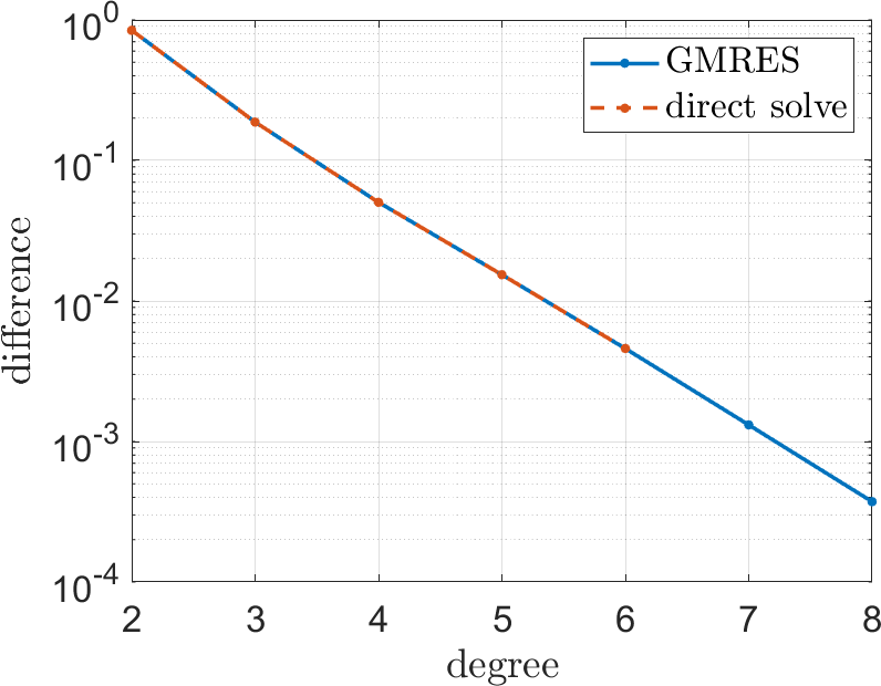
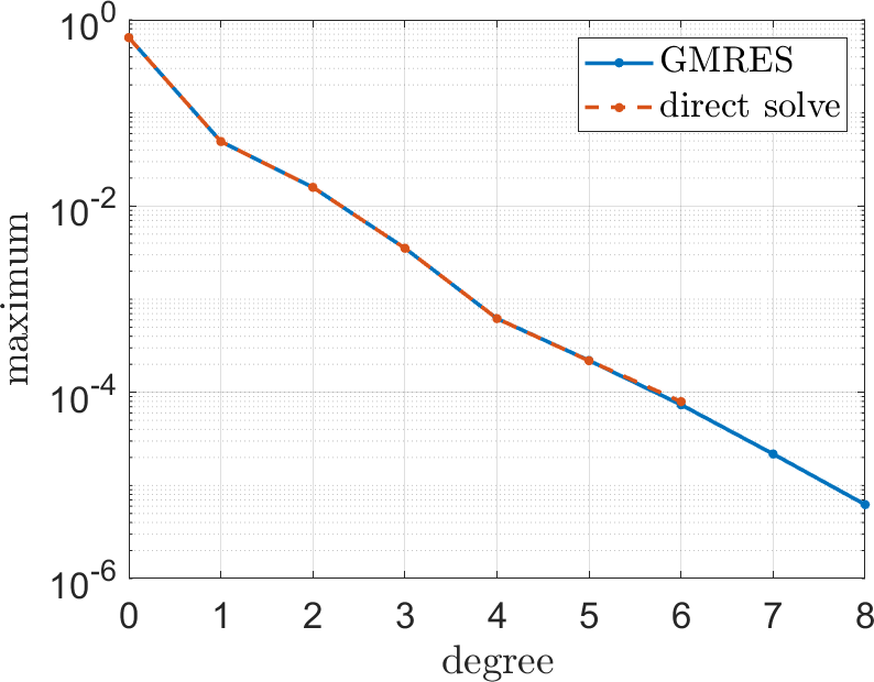
Figure 12: Left: Euclidean norms $\lVert x_{r-1}-x_{r}\rVert_{2}$ as a function of the polynomial degree $r=2,\ldots,8$, where $x_{r}$ is the solution of $Ax=b$ using total degree $r$ in the stochastic Galerkin method. Right: Magnitudes (7.6) as a function of the degree $j$.

Denote by $x_{r}$ the solution of $Ax=b$ when using polynomials of degree up to $r$ in the stochastic Galerkin method, where the number of basis polynomials is given in (7.3). The left panel of Figure 12 displays the differences $\lVert x_{r-1}-x_{r}\rVert_{2}$ as a function of $r$ (the vector $x_{r-1}$ is padded with zeros at the end to match the size of $x_{r}$). Their exponential decay suggests convergence of the stochastic Galerkin method.

Next, we fix the degree $r=8$ in the stochastic Galerkin method. Recall from (3.5) and (3.8) that the solution of $Ax=b$ contains the coefficient vectors $V_{0},\ldots,V_{m}$ of the polynomials $\phi_{0},\ldots,\phi_{m}$ in the stochastic Galerkin method. We also examine the largest maximum norm of the coefficients associated to polynomials of total degree (exactly) $j$, i.e., the values

$$\gamma_{j}=\max\left\{\lVert V_{i}\rVert_{\infty}:\,\deg(\phi_{i})=j\right\}.$$ (7.6)

The right panel of Figure 12 shows the magnitudes (7.6) for $j=0,1,\ldots,8$. The observed exponential decay stems from the exponential convergence of (2.7), since the wavenumber in (7.1) is analytic in $\xi_{1},\xi_{2},\xi_{3}$.

We repeat this experiment with $\theta=0.2$ instead of $\theta=0.1$. Overall, the behavior is similar as for $\theta=0.1$, but convergence is slower: the relative residual norms reach the prescribed tolerance in $60$ instead of $20$ iteration steps, and also $\lVert x_{r-1}-x_{r}\rVert_{2}$ as well as the magnitudes (7.6) converge more slowly.

8 Conclusions

We investigated the Helmholtz equation including a random wavenumber. The combination of a stochastic Galerkin method and a finite difference method yielded a high-dimensional linear system of algebraic equations. We examined the iterative solution of these linear systems using three types of preconditioners: a complex shifted Laplace preconditioner, a mean value preconditioner, and a combined variant. Theoretical properties of the preconditioned linear systems were shown. Numerical computations demonstrate that the straightforward mean value preconditioner provides the most efficient iterative solution within these types.

Appendix A Discretizations

A.1 Finite differences and stochastic Galerkin method in 1D

Consider the grid of equispaced points

$$x_{j}=jh,\quad j=0,1,\ldots,q+1,$$ (A.1)

in $\overline{Q}=[0,1]$ with mesh-size $h=1/(q+1)$. For brevity of notation, set

$$u_{j}(\xi)\coloneq u(x_{j},\xi),\quad k_{j}(\xi)\coloneq k(x_{j},\xi),\quad f_{j}\coloneq f(x_{j}),\quad j=0,1,\ldots,q+1.$$ (A.2)

A finite difference discretization of the Helmholtz equation (3.1) using second order central differences yields

$$\frac{1}{h^{2}}\Bigl{(}-u_{j-1}(\xi)+2u_{j}(\xi)-u_{j+1}(\xi)\Bigr{)}-k_{j}(\xi)^{2}u_{j}(\xi)=f_{j},\quad j=1,\ldots,q.$$ (A.3)

This discretization is consistent of order two. Since $u_{0}(\xi)=u_{q+1}(\xi)=0$ for all $\xi\in\Xi$ in the case of homogeneous Dirichlet boundary conditions, we obtain the following discretization.

Theorem A.1.

In the above notation, the Helmholtz equation (3.1) on $Q=]0,1[$ with homogeneous Dirichlet boundary conditions has the second order FD discretization

$$S(\xi)U(\xi)=F_{0},\quad U(\xi)=\begin{bmatrix}u_{1}(\xi)\\ \vdots\\ u_{q}(\xi)\end{bmatrix}\in\mathbb{R}^{q},\quad F_{0}=\begin{bmatrix}f_{1}\\ \vdots\\ f_{q}\end{bmatrix}\in\mathbb{R}^{q},$$ (A.4)

with the matrix

$$S(\xi)=T-D(\xi)\in\mathbb{R}^{q,q},$$ (A.5)

where $T$ is the discretization of the Dirichlet Laplacian,

$$T =\frac{1}{h^{2}}\begin{bmatrix}2&-1\\ -1&2&-1\\ &\ddots&\ddots&\ddots\\ &&-1&2&-1\\ &&&-1&2\end{bmatrix},$$ (A.6)

$$D(\xi) =\operatorname{diag}\big{(}k_{1}(\xi)^{2},\ldots,k_{q}(\xi)^{2}\big{)}.$$ (A.7)

The matrices $T$ and $D(\xi)$ are symmetric positive definite.

Moreover, the coefficient vectors of the stochastic Galerkin approximation (3.5) are solutions of the linear algebraic system

$$AV=\begin{bmatrix}F_{0}\\ \vdots\\ F_{m}\end{bmatrix},\quad V=\begin{bmatrix}V_{0}\\ \vdots\\ V_{m}\end{bmatrix},$$ (A.8)

where $F_{i}=0\in\mathbb{R}^{q}$ for $i=1,\ldots,m$, and

$$A=I_{m+1}\otimes T-\begin{bmatrix}C_{ij}\end{bmatrix}\in\mathbb{R}^{(m+1)q,(m+1)q},$$ (A.9)

where

$$C_{ij}\coloneq\langle D(\xi)\phi_{j}(\xi),\phi_{i}(\xi)\rangle=\operatorname{diag}\Big{(}\langle k_{1}(\xi)^{2}\phi_{j}(\xi),\phi_{i}(\xi)\rangle,\ldots,\langle k_{q}(\xi)^{2}\phi_{j}(\xi),\phi_{i}(\xi)\rangle\Big{)}$$ (A.10)

for $i,j=0,\ldots,m$. The matrices $I_{m+1}\otimes T$ and $\begin{bmatrix}C_{ij}\end{bmatrix}$ are symmetric positive definite.

Proof.

The matrix $T$ is symmetric positive definite by [14, Lem. 6.1] and $D(\xi)$ is symmetric positive definite since $k(x,\xi)>0$ for all $x$ and $\xi$ by assumption.

The coefficient vectors $V_{0},\ldots,V_{m}$ are determined from the orthogonality condition (3.7), i.e., $\langle S(\xi)\widetilde{U}_{m}(\xi),\phi_{i}(\xi)\rangle=\delta_{i,0}F_{0}$, $i=0,1,\ldots,m$. Inserting $\widetilde{U}_{m}(\xi)$ from (3.5) and $S(\xi)$ from (A.5) in the left hand side yields

$$\langle S(\xi)\widetilde{U}_{m}(\xi),\phi_{i}(\xi)\rangle =\sum_{j=0}^{m}\langle\phi_{j}(\xi)TV_{j},\phi_{i}(\xi)\rangle-\sum_{j=0}^{m}\langle\phi_{j}(\xi)D(\xi)V_{j},\phi_{i}(\xi)\rangle$$ (A.11)

$$=TV_{i}-\sum_{j=0}^{m}C_{ij}V_{j},$$ (A.12)

see Lemma 3.2 and Corollary 3.3, which shows that $A$ has the form (A.9). Moreover, since $T$ and $D(\xi)$ are symmetric positive definite, also $I_{m+1}\otimes T$ and $\begin{bmatrix}C_{ij}\end{bmatrix}$ are symmetric positive definite by Lemma 3.2. ∎

The absorbing boundary conditions for $Q=]0,1[$ are

$$-u^{\prime}(0,\xi)-{\operatorname{i}}k(0,\xi)u(0,\xi)=0,\quad u^{\prime}(1,\xi)-{\operatorname{i}}k(1,\xi)u(1,\xi)=0\quad\text{for }\xi\in\Xi.$$ (A.13)

We obtain a second order approximation of $u^{\prime}$ in the boundary points as described in [14, Sect. 6.4.1]. A Taylor expansion in $x_{0}=0$ yields

$$u(x_{1},\xi) =u(x_{0},\xi)+hu^{\prime}(x_{0},\xi)+\frac{h^{2}}{2}u^{\prime\prime}(x_{0},\xi)+O(h^{3})$$ (A.14)

$$=u(x_{0},\xi)+hu^{\prime}(x_{0},\xi)-\frac{h^{2}}{2}\Big{(}k(x_{0},\xi)u(x_{0},\xi)+f(x_{0})\Big{)}+O(h^{3}),$$ (A.15)

where we replaced $u^{\prime\prime}$ using the Helmholtz equation. This yields a second order approximation of $u^{\prime}(x_{0},\xi)$. Inserting it in (A.13) and dividing by $h$ yields the discretization

$$\frac{u_{0}(\xi)-u_{1}(\xi)}{h^{2}}-\frac{{\operatorname{i}}}{h}k_{0}(\xi)u_{0}(\xi)-\frac{k_{0}(\xi)^{2}}{2}u_{0}(\xi)=\frac{f_{0}}{2}.$$ (A.16)

Similarly, the absorbing boundary condition in $x_{q+1}=1$ is discretized by

$$\frac{-u_{q}(\xi)+u_{q+1}(\xi)}{h^{2}}-\frac{{\operatorname{i}}}{h}k_{q+1}(\xi)u_{q+1}(\xi)-\frac{k_{q+1}(\xi)^{2}}{2}u_{q+1}(\xi)=\frac{f_{q+1}}{2}.$$ (A.17)

The approximation is consistent of order two. It leads to the following discretization.

Theorem A.2.

In the above notation, the Helmholtz equation (3.1) on $Q=]0,1[$ with absorbing boundary conditions has the second order FD discretization

$$S(\xi)U(\xi)=F_{0},\quad U(\xi)=\begin{bmatrix}u_{0}(\xi)\\ u_{1}(\xi)\\ \vdots\\ u_{q}(\xi)\\ u_{q+1}(\xi)\end{bmatrix}\in\mathbb{R}^{q+2},\quad F_{0}=\begin{bmatrix}f_{0}/2\\ f_{1}\\ \vdots\\ f_{q}\\ f_{q+1}/2\end{bmatrix}\in\mathbb{R}^{q+2},$$ (A.18)

with the matrix

$$S(\xi)=T-{\operatorname{i}}D_{1}(\xi)-D_{2}(\xi)\in\mathbb{C}^{q+2,q+2}$$ (A.19)

and real

$$T =\frac{1}{h^{2}}\begin{bmatrix}1&-1\\ -1&2&-1\\ &\ddots&\ddots&\ddots\\ &&-1&2&-1\\ &&&-1&1\end{bmatrix},$$ (A.20)

$$D_{1}(\xi) =\frac{1}{h}\operatorname{diag}\Big{(}k_{0}(\xi),0,\ldots,0,k_{q+1}(\xi)\Big{)},$$ (A.21)

$$D_{2}(\xi) =\operatorname{diag}\bigg{(}\frac{k_{0}(\xi)^{2}}{2},k_{1}(\xi)^{2},\ldots,k_{q}(\xi)^{2},\frac{k_{q+1}(\xi)^{2}}{2}\bigg{)}.$$ (A.22)

The matrices $T,D_{1}(\xi)$ are symmetric positive semidefinite (for all $\xi\in\Xi$), and $\ker(T)=\operatorname{span}\{[1,\ldots,1]^{\top}\}$. The matrix $D_{2}(\xi)$ is symmetric positive definite for all $\xi\in\Xi$.

Moreover, the coefficient vectors of the stochastic Galerkin approximation (3.5) are solutions of the linear algebraic system

$$AV=\begin{bmatrix}F_{0}\\ \vdots\\ F_{m}\end{bmatrix},\quad V=\begin{bmatrix}V_{0}\\ \vdots\\ V_{m}\end{bmatrix},$$ (A.23)

where $F_{i}=0\in\mathbb{R}^{q+2}$ for $i=1,\ldots,m$, and

$$A=I_{m+1}\otimes T-{\operatorname{i}}[B_{ij}]-[C_{ij}]\in\mathbb{C}^{(m+1)(q+2),(m+1)(q+2)}$$ (A.24)

with

$$B_{ij} \coloneq\frac{1}{h}\operatorname{diag}\Bigl{(}\langle k_{0}\phi_{j},\phi_{i}\rangle,0,\ldots,0,\langle k_{q+1}\phi_{j},\phi_{i}\rangle\Bigr{)},$$ (A.25)

$$C_{ij} \coloneq\operatorname{diag}\Bigl{(}\frac{1}{2}\langle k_{0}^{2}\phi_{j},\phi_{i}\rangle,\langle k_{1}^{2}\phi_{j},\phi_{i}\rangle,\ldots,\langle k_{q}^{2}\phi_{j},\phi_{i}\rangle,\frac{1}{2}\langle k_{q+1}^{2}\phi_{j},\phi_{i}\rangle\Bigr{)}$$ (A.26)

for $i,j=0,\ldots,m$. Note that $B_{ij},C_{ij}\in\mathbb{R}^{q+2,q+2}$. The matrices $I_{m+1}\otimes T$ and $\begin{bmatrix}B_{ij}\end{bmatrix}$ are symmetric positive semidefinite, the matrix $\begin{bmatrix}C_{ij}\end{bmatrix}$ is symmetric positive definite.

Proof.

The form of $S(\xi)$ in (A.19) follows from the finite difference discretization described above. To show that $T$ is symmetric positive definite, we make use of the Sturm sequence property of $-h^{2}T$, which is a Jacobi matrix (real, symmetric, tridiagonal, with positive off-diagonal elements). For $j=1,\ldots,q+2$, denote by $T_{j}$ the upper left $j\times j$ block of $h^{2}T$. Then $\det(T_{1})=1$, $\det(T_{2})=1$ and, by induction, $\det(T_{j})=2\det(T_{j-1})-\det(T_{j-2})$ for $j=3,\ldots,q+1$, which shows $\det(T_{j})=1$ for $j=1,\ldots,q+1$. Finally, $\det(T_{q+2})=\det(T_{q+1})-\det(T_{q})=0$. Thus, the determinants $\det(-T_{j})=(-1)^{j}$ alternate for $j=1,\ldots,q+1$ while $\det(-T_{q+2})=0$, so that there is only one “agreement in sign” from the final $0$ in the Sturm sequence for $-h^{2}T$, showing that $-h^{2}T$ has exactly one nonnegative eigenvalue, namely $0$. Therefore, $T$ has one eigenvalue $0$ and all other eigenvalues of $T$ are positive. The rest is very similar to the proof of Theorem A.1. ∎

Lemma A.3.

In the notation of Theorem A.2, if $\xi$ is a random variable that is uniformly distributed in $[-1,1]$ and if $k(x,\xi)$ is a polynomial in $\xi$ of degree at most $n$ for all $x\in Q$, then $B_{ij}=0$ for $\lvert i-j\rvert>n$ and $C_{ij}=0$ for $\lvert i-j\rvert>2n$.

Proof.

The proof relies on the fact of orthogonal polynomials, that $\langle p,\phi_{j}\rangle=0$ for all polynomials with $\deg(p)<j$. If $\deg_{\xi}(k(x,\xi))\leq n$, then $\langle k(x,\xi)\phi_{i}(\xi),\phi_{j}\rangle=0$ for $i+n<j$, i.e., $i-j<-n$. Since $k$ is real, we also have $\langle k(x,\xi)\phi_{i}(\xi),\phi_{j}\rangle=\langle\phi_{i}(\xi),k(x,\xi)\phi_{j}\rangle=0$ for $n+j<i$, i.e., $i-j>n$. This shows that $B_{ij}=0$ for $\lvert i-j\rvert>n$. Similarly $C_{ij}=0$ for $\lvert i-j\rvert>2n$ since $\deg_{\xi}(k(x,\xi)^{2})=2n$. ∎

If the wavenumber is constant in space, the matrices $[B_{ij}]$ and $[C_{ij}]$ simplify, as indicated in the next lemma.

Lemma A.4.

In the notation of Theorem A.2, if the wavenumber is constant in space, i.e., $k(x,\xi)=k(\xi)$, then

$$B_{ij} =\langle k(\xi)\phi_{j}(\xi),\phi_{i}(\xi)\rangle D_{1},\quad D_{1}=\frac{1}{h}\operatorname{diag}\big{(}1,0,\ldots,0,1\big{)},$$ (A.27)

$$C_{ij} =\langle k(\xi)^{2}\phi_{j}(\xi),\phi_{i}(\xi)\rangle D_{2},\quad D_{2}=\operatorname{diag}\Bigr{(}\frac{1}{2},1,\ldots,1,\frac{1}{2}\Bigr{)},$$ (A.28)

so that

$$[B_{ij}]=[\langle k(\xi)\phi_{j}(\xi),\phi_{i}(\xi)\rangle]_{ij}\otimes D_{1},\quad[C_{ij}]=[\langle k(\xi)^{2}\phi_{j}(\xi),\phi_{i}(\xi)\rangle]_{ij}\otimes D_{2}.$$ (A.29)

Lemma A.3 and Lemma A.4 also hold in the setting of Theorem A.1 with the obvious modifications.

A.2 Finite differences and stochastic Galerkin method in 2D

We discretize the stochastic Helmholtz equation (3.1) on $Q=]0,1[^{2}$. Let $q\in\mathbb{N}$. We discretize $[0,1]^{2}$ by the grid

$$(x_{i},y_{j})=(ih,jh),\quad i,j=0,1,\ldots,q+1,$$ (A.30)

with mesh-size $h=1/(q+1)$. For brevity of notation, set

$$u_{i,j}=u(x_{i},y_{j},\xi),\quad k_{i,j}=k(x_{i},y_{j},\xi),\quad f_{i,j}=f(x_{i},y_{j}),\quad i,j=0,1,\ldots,q+1.$$ (A.31)

Discretizing the Laplacian with the $5$-point stencil leads to

$$\frac{1}{h^{2}}(-u_{i-1,j}+2u_{i,j}-u_{i+1,j}-u_{i,j-1}+2u_{i,j}-u_{i,j+1})-k_{i,j}^{2}u_{i,j}=f_{i,j}$$ (A.32)

for $i,j=1,\ldots,N$. This discretization is consistent of order two.

Theorem A.5.

In the above notation, the stochastic Helmholtz equation (3.1) on $Q=]0,1[^{2}$ with homogeneous Dirichlet boundary conditions has the second order FD discretization

$$S(\xi)U(\xi)=b_{0},$$ (A.33)

where the function values are ordered as

$$U(\xi) =[u_{1,1},u_{2,1},\ldots,u_{q,1},u_{1,2},\ldots,u_{q,2},\ldots,u_{1,q},\ldots,u_{q,q}]^{\top}\in\mathbb{R}^{q^{2}},\quad\xi\in\Xi,$$ (A.34)

$$b_{0} =[f_{1,1},f_{2,1},\ldots,f_{q,1},f_{1,2},\ldots,f_{q,2},\ldots,f_{1,q},\ldots,f_{q,q}]^{\top}\in\mathbb{R}^{q^{2}},$$ (A.35)

the matrix is given by

$$S(\xi)=L-D_{2}(\xi)\in\mathbb{R}^{q^{2},q^{2}},$$ (A.36)

and

$$L =I_{q}\otimes T+T\otimes I_{q},$$ (A.37)

$$D_{2}(\xi) =\operatorname{diag}(k_{1,1}^{2},\ldots,k_{q,1}^{2},k_{1,2}^{2},\ldots,k_{q,2}^{2},\ldots,k_{1,q}^{2},\ldots,k_{q,q}^{2})$$ (A.38)

with $T$ from (A.6). The matrices $L$ and $D_{2}(\xi)$ are symmetric positive definite.

Moreover, the coefficient vectors of the stochastic Galerkin approximation (3.5) are solutions of the linear algebraic system

$$AV=b,\quad V=\begin{bmatrix}V_{0}\\ \vdots\\ V_{m}\end{bmatrix},\quad b=\begin{bmatrix}b_{0}\\ \vdots\\ b_{m}\end{bmatrix},$$ (A.39)

where $b_{i}=0\in\mathbb{R}^{q^{2}}$ for $i=1,\ldots,m$, and

$$A=I_{m+1}\otimes L-\begin{bmatrix}C_{ij}\end{bmatrix}\in\mathbb{R}^{(m+1)q^{2},(m+1)q^{2}},$$ (A.40)

where

$$C_{ij}\coloneq\operatorname{diag}\Bigl{(}\langle k_{1,1}^{2}\phi_{i},\phi_{j}\rangle,\ldots,\langle k_{q,1}^{2}\phi_{i},\phi_{j}\rangle,\ldots,\langle k_{1,q}^{2}\phi_{i},\phi_{j}\rangle,\ldots,\langle k_{q,q}^{2}\phi_{i},\phi_{j}\rangle\Bigr{)}$$ (A.41)

for $i,j=0,\ldots,m$. The matrices $I_{m+1}\otimes L$ and $\begin{bmatrix}C_{ij}\end{bmatrix}$ are symmetric positive definite.

To obtain a second order discretization of absorbing boundary conditions, we proceed as described in [14, Sect. 10.2.1]. This leads to the following result.

Theorem A.6.

In the above notation, the Helmholtz equation (3.1) on $Q=]0,1[^{2}$ with absorbing boundary conditions has the second order FD discretization

$$S(\xi)U(\xi)=b_{0},$$ (A.42)

where the right hand side is

$$b_{0}=\begin{bmatrix}\frac{1}{2}F_{0}\\ F_{1}\\ \vdots\\ F_{N}\\ \frac{1}{2}F_{q+1}\end{bmatrix}\in\mathbb{R}^{(q+2)^{2}},\quad F_{j}=\begin{bmatrix}\frac{1}{2}f_{0,j}\\ f_{1,j}\\ \vdots\\ f_{q,j}\\ \frac{1}{2}f_{q+1,j}\end{bmatrix}\in\mathbb{R}^{q+2},\quad 0\leq j\leq q+1,$$ (A.43)

and where the matrix is given by

$$S(\xi)=L-{\operatorname{i}}D_{1}(\xi)-D_{2}(\xi)\in\mathbb{C}^{(q+2)^{2},(q+2)^{2}}$$ (A.44)

with block matrices

$$L =D\otimes T+T\otimes D,$$ (A.45)

$$D_{1}(\xi) =\frac{1}{h}\operatorname{diag}\Bigl{(}D_{1,0}(\xi),D_{1,1}(\xi),\ldots,D_{1,q}(\xi),D_{1,q+1}(\xi)\Bigr{)},$$ (A.46)

$$D_{2}(\xi) =\operatorname{diag}\Bigl{(}\frac{1}{2}D_{2,0}(\xi),D_{2,1}(\xi),\ldots,D_{2,q}(\xi),\frac{1}{2}D_{2,q+1}(\xi)\Bigr{)},$$ (A.47)

and $(q+2)\times(q+2)$-blocks $T$ from (A.20),

$$D =\operatorname{diag}\Bigl{(}\frac{1}{2},1,\ldots,1,\frac{1}{2}\Bigr{)},$$ (A.48)

$$D_{1,j}(\xi) =\begin{cases}\operatorname{diag}(k_{0,j},k_{1,j},\ldots,k_{q,j},k_{q+1,j}),&j=0,q+1,\\ \operatorname{diag}(k_{0,j},0,\ldots,0,k_{q+1,j}),&j=1,\ldots,q,\end{cases}$$ (A.49)

$$D_{2,j}(\xi) =\operatorname{diag}\Big{(}\frac{1}{2}k_{0,j}^{2},k_{1,j}^{2},\ldots,k_{q,j}^{2},\frac{1}{2}k_{q+1,j}^{2}\Big{)},\quad j=0,1,\ldots,q+1.$$ (A.50)

The matrices $L$, $D_{1}(\xi)$ are symmetric positive semidefinite (for all $\xi\in\Xi$). The matrix $D_{2}(\xi)$ is symmetric positive definite for all $\xi\in\Xi$.

Moreover, the coefficient vectors of the stochastic Galerkin approximation (3.5) are solutions of the linear algebraic system

$$AV=b,\quad b=\begin{bmatrix}b_{0}\\ \vdots\\ b_{m}\end{bmatrix},\quad V=\begin{bmatrix}V_{0}\\ \vdots\\ V_{m}\end{bmatrix},$$ (A.51)

where $b_{i}=0\in\mathbb{R}^{(q+2)^{2}}$ for $i=1,\ldots,m$, and

$$A=I_{m+1}\otimes L-{\operatorname{i}}[B_{ij}]-[C_{ij}]\in\mathbb{C}^{(m+1)(q+2)^{2},(m+1)(q+2)^{2}}$$ (A.52)

with

$$B_{ij}\coloneq\langle D_{1}(\xi)\phi_{i}(\xi),\phi_{j}(\xi)\rangle,\quad C_{ij}\coloneq\langle D_{2}(\xi)\phi_{i}(\xi),\phi_{j}(\xi)\rangle\in\mathbb{R}^{(q+2)^{2},(q+2)^{2}}$$ (A.53)

for $i,j=0,\ldots,m$. The matrices $I_{m+1}\otimes L$ and $\begin{bmatrix}B_{ij}\end{bmatrix}$ are symmetric positive semidefinite, the matrix $\begin{bmatrix}C_{ij}\end{bmatrix}$ is symmetric positive definite.

A.3 Point sources

The source term $f$ in the Helmholtz equation is often a point source, typically represented by a Dirac delta distribution, say $f(x)=\delta(x-a)$. In our finite difference approximation in one dimension, we discretize $f$ by $1/h$ at $a$ (or at a grid point with smallest distance to $a$) and $0$ at the other grid points; see also [28] for a discussion of the discretization of the Dirac distribution. In two space dimension, we discretize $f(x)=\delta(x-a)$ by $1/h^{2}$ at $a$ (or at a closest grid point).

Specifically for $f(x)=\delta(x-1/2)$ and the grid (A.1) or $\delta((x,y)-(1/2,1/2))$ and the grid (A.30), let $t=\lceil q/2\rceil=\lfloor(q+1)/2\rfloor$. If $q$ is odd, $x_{t}=1/2$ is the exact midpoint. If $q$ is even, $t=q/2$ and $x_{t}=1/2-h/2$ is the smaller of the two grid points closest to $1/2$. We then discretize $f$ by

$$f(x_{j})=\begin{cases}1/h,&j=t,\\ 0,&j\neq t,\end{cases}\quad\text{or}\quad f(x_{j},y_{\ell})=\begin{cases}1/h^{2},&j=\ell=t,\\ 0,&\text{else.}\end{cases}$$ (A.54)

A.4 Stochastic Galerkin and finite differences in 1D

We discretize the deterministic system of PDEs obtained from the stochastic Helmholtz equation with the the stochastic Galerkin method as described in Section 3.2.

We first discretize the PDE (3.18) with the grid (A.1). We have

$$-v_{j}^{\prime\prime}(x)-\sum_{i=0}^{m}c_{ij}(x)v_{i}(x)=F_{j}(x),\quad x\in Q=]0,1[,\quad j=0,1,\ldots,m.$$ (A.55)

Second order central differences yield the approximation

$$\frac{1}{h^{2}}(-v_{j}(x_{\ell-1})+2v_{j}(x_{\ell})-v_{j}(x_{\ell+1}))-\sum_{i=0}^{m}c_{ij}(x_{\ell})v_{i}(x_{\ell})=F_{j}(x_{\ell}),\quad\ell=1,\ldots,q.$$ (A.56)

Given homogeneous Dirichlet boundary conditions (3.19), we order the unknowns as

$$V=[v_{0}(x_{1}),\ldots,v_{0}(x_{q}),v_{1}(x_{1}),\ldots,v_{1}(x_{q}),\ldots,v_{m}(x_{1}),\ldots,v_{m}(x_{q})]^{\top}.$$ (A.57)

Then (A.56) yields the block system (A.9). The boundary conditions (3.23) are

$$-v_{j}^{\prime}(0)-{\operatorname{i}}\sum_{i=0}^{m}b_{ij}(0)v_{i}(0)=0,\quad v_{j}^{\prime}(1)-{\operatorname{i}}\sum_{i=0}^{m}b_{ij}(1)v_{i}(1)=0,\quad j=0,1,\ldots,m.$$ (A.58)

A second order discretization of $v_{j}^{\prime}$ is derived as in (A.15). Ordering the unknowns as

$$V=[v_{0}(x_{0}),\ldots,v_{0}(x_{q+1}),v_{1}(x_{0}),\ldots,v_{1}(x_{q+1}),\ldots,v_{m}(x_{0}),\ldots,v_{m}(x_{q+1})]^{\top}$$ (A.59)

yields the block system (A.23).

References

- [1] T. Airaksinen, E. Heikkola, A. Pennanen, and J. Toivanen, An algebraic multigrid based shifted-Laplacian preconditioner for the Helmholtz equation, J. Comput. Phys., 226 (2007), pp. 1196–1210.
- [2] D. Colton and R. Kress, Inverse Acoustic and Electromagnetic Scattering Theory, Springer, New York, 3rd ed., 2013.
- [3] S. Cools and W. Vanroose, Local Fourier analysis of the complex shifted Laplacian preconditioner for Helmholtz problems, Numer. Linear Algebra Appl., 20 (2013), pp. 575–597.
- [4] T. A. Davis, UMFPACK user guide (version 5.7.7), tech. rep., 2018.
- [5] Y. A. Erlangga, Advances in iterative methods and preconditioners for the Helmholtz equation, Arch. Comput. Methods Eng., 15 (2008), pp. 37–66.
- [6] Y. A. Erlangga, C. Vuik, and C. W. Oosterlee, On a class of preconditioners for solving the Helmholtz equation, Appl. Numer. Math., 50 (2004), pp. 409–425.
- [7] M. J. Gander, I. G. Graham, and E. A. Spence, Applying GMRES to the Helmholtz equation with shifted Laplacian preconditioning: what is the largest shift for which wavenumber-independent convergence is guaranteed?, Numer. Math., 131 (2015), pp. 567–614.
- [8] L. García Ramos and R. Nabben, On the spectrum of deflated matrices with applications to the deflated shifted Laplace preconditioner for the Helmholtz equation, SIAM J. Matrix Anal. Appl., 39 (2018), pp. 262–286.
- [9] L. García Ramos, O. Sète, and R. Nabben, Preconditioning the Helmholtz equation with the shifted Laplacian and Faber polynomials, Electron. Trans. Numer. Anal., 54 (2021), pp. 534–557.
- [10] R. G. Ghanem and R. M. Kruger, Numerical solution of spectral stochastic finite element systems, Comput. Meth. Appl. Mech. Engrg., 129 (1996), pp. 289–303.
- [11] R. G. Ghanem and P. D. Spanos, Stochastic finite elements: a spectral method approach, Springer, New York, 1991.
- [12] C. J. Gittelson, An adaptive stochastic Galerkin method for random elliptic operators, Math. Comput., 82 (2013), pp. 1515–1541.
- [13] D. Gottlieb and D. Xiu, Galerkin method for wave equations with uncertain coefficients, Comm. Comput. Phys., 3 (2008), pp. 505–518.
- [14] D. F. Griffiths, J. W. Dold, and D. J. Silvester, Essential partial differential equations, Springer Undergraduate Mathematics Series, Springer, Cham, 2015.
- [15] C. Grossmann, H.-G. Roos, and M. Stynes, Numerical Treatment of Partial Differential Equations, Springer, Berlin, 2007.
- [16] F. Ihlenburg, Finite element analysis of acoustic scattering, vol. 132 of Applied Mathematical Sciences, Springer-Verlag, New York, 1998.
- [17] D. Lahaye, J. Tang, and K. Vuik, eds., Modern solvers for Helmholtz problems, Birkhäuser/Springer, Cham, 2017.
- [18] I. Livshits, Use of shifted Laplacian operators for solving indefinite Helmholtz equations, Numer. Math. Theory Methods Appl., 8 (2015), pp. 136–148.
- [19] A. D. Polyanin, Handbook of Linear Partial Differential Equations for Engineers and Scientists, Chapman & Hall/CRC, 2002.
- [20] R. Pulch, Stability-preserving model order reduction for linear stochastic Galerkin systems, J. Math. Ind., 9 (2019), pp. Paper No. 10, 24.
- [21] R. Pulch and C. van Emmerich, Polynomial chaos for simulating random volatilities, Math. Comput. Simulation, 80 (2009), pp. 245–255.
- [22] R. Pulch and D. Xiu, Generalised polynomial chaos for a class of linear conservation laws, J. Sci. Comput., 51 (2012), pp. 293–312.
- [23] B. Reps, W. Vanroose, and H. bin Zubair, On the indefinite Helmholtz equation: complex stretched absorbing boundary layers, iterative analysis, and preconditioning, J. Comput. Phys., 229 (2010), pp. 8384–8405.
- [24] Y. Saad and M. H. Schultz, GMRES: a generalized minimal residual algorithm for solving nonsymmetric linear systems, SIAM J. Sci. Statist. Comput., 7 (1986), pp. 856–869.
- [25] A. H. Sheikh, D. Lahaye, L. Garcia Ramos, R. Nabben, and C. Vuik, Accelerating the shifted Laplace preconditioner for the Helmholtz equation by multilevel deflation, J. Comput. Phys., 322 (2016), pp. 473–490.
- [26] J. Stoer and R. Bulirsch, Introduction to Numerical Analysis, Springer Science+Business Media, New York, 3rd ed., 2002.
- [27] M. B. van Gijzen, Y. A. Erlangga, and C. Vuik, Spectral analysis of the discrete Helmholtz operator preconditioned with a shifted Laplacian, SIAM J. Sci. Comput., 29 (2007), pp. 1942–1958.
- [28] D. Wang, J.-H. Jung, and G. Biondini, Detailed comparison of numerical methods for the perturbed sine-Gordon equation with impulsive forcing, J. Engrg. Math., 87 (2014), pp. 167–186.
- [29] G. Wang, F. Xue, and Q. Liao, Localized stochastic Galerkin methods for Helmholtz problems close to resonance, Int. J. Uncertainty Quantification, 11 (2021), pp. 77–99.
- [30] D. Xiu, Numerical methods for stochastic computations: a spectral method approach, Princeton University Press, Princeton, NJ, 2010.
- [31] D. Xiu and J. Shen, Efficient stochastic Galerkin methods for random diffusion equations, J. Comput. Phys., 228 (2009), pp. 266–281.
- [32] M. Youssef and R. Pulch, Poly-Sinc solution of stochastic elliptic differential equations, J. Sci. Comput., 87 (2021). Paper No. 82.