Probing Early Universe Supercooled Phase Transitions with Gravitational Wave Data

Abstract

We investigate the reach of the LIGO/Virgo/KAGRA detectors in the search for signatures of first-order phase transitions in the early Universe. Utilising data from the first three observing runs, we derive constraints on the parameters of the underlying gravitational-wave background, focusing on transitions characterised by strong supercooling. As an application of our analysis, we determine bounds on the parameter space of two representative particle physics models. We also comment on the expected reach of third-generation detectors in probing supercooled phase transitions.

I Introduction

The 2015 discovery of gravitational waves (GWs) by the LIGO/Virgo collaboration, based on the data obtained at the twin LIGO detectors Abbott et al. (2016) gave rise to the field of GW astronomy. Since then, as many as $\mathcal{O}$(100) GW signals have been recorded Abbott et al. (2021a, b). Those events include binary black hole mergers, binary neutron star mergers, and a black hole-neutron star merger. Apart from such individually detectable events, a GW background is also expected to be discovered with increased detector sensitivity. One contribution to this background arises from the superposition of unresolved astrophysical sources Christensen (2019). However, a more intriguing possibility is a contribution of cosmological origin. Several processes would give rise to such a cosmological GW background, including first order phase transitions (FOPTs) in the early Universe Kosowsky et al. (1992), inflation Turner (1997), or topological defects such as cosmic strings Vachaspati and Vilenkin (1985); Sakellariadou (1990) and domain walls Hiramatsu et al. (2014). In this work, we concentrate on the expected signatures from FOPTs.

Although the particle content of the Standard Model (SM) alone is not sufficient for a FOPT to occur in the early Universe, FOPTs are a generic feature in a number of theories beyond the SM. Some examples include models with new physics at the electroweak scale Grojean and Servant (2007); Vaskonen (2017); Dorsch et al. (2017); Chala et al. (2018); Alves et al. (2019), hidden sectors Schwaller (2015); Breitbach et al. (2019); Croon et al. (2018); Hall et al. (2020), dark matter Hambye et al. (2018); Baldes and Garcia-Cely (2019); Baldes et al. (2022a); Azatov et al. (2021a); Baldes et al. (2022b), unification Croon et al. (2019); Brdar et al. (2019a); Huang et al. (2020); Okada et al. (2021), confinement Helmboldt et al. (2019); Croon et al. (2020); Huang et al. (2021), baryon and/or lepton number violation Cheung et al. (2012); Katz and Riotto (2016); Hasegawa et al. (2019); Fornal and Shams Es Haghi (2020); Baldes et al. (2021); Azatov et al. (2021b)), neutrino mass models Brdar et al. (2019b); Okada and Seto (2018); Di Bari et al. (2021); Zhou et al. (2022), axions Dev et al. (2019); Von Harling et al. (2020); Delle Rose et al. (2020), supersymmetry breaking Demidov et al. (2018); Craig et al. (2020); Fornal et al. (2021), or theories explaining flavour anomalies Greljo et al. (2020); Fornal (2021). [For a more complete list of references on models exhibiting FOPTs, we refer the reader to Caldwell et al. (2022).]

This interplay between particle physics and GWs provides a unique opportunity to explore regions of parameter space otherwise unreachable in typical particle physics experiments. Indeed, the new physics energy scales $\gtrsim 100\ {\rm TeV}$ fall outside the range probed by Earth-based accelerators. However, precisely such large energy scales can give rise to a signal within the frequency range of the LIGO/Virgo/KAGRA (LVK) detectors, since the peak frequency is expected to fall within the range $\sim(10-1000)$ Hz.

A particularly interesting scenario is when the FOPT is supercooled, which often increases the duration of the FOPT, leading to an enhancement of the GW signal. A prolonged period of supercooling can arise in theories with Coleman-Weinberg-type symmetry breaking Coleman and Weinberg (1973) or in strongly-coupled scenarios. Some models of this type are discussed in Creminelli et al. (2002); Randall and Servant (2007); Nardini et al. (2007); Konstandin and Servant (2011); Jinno and Takimoto (2017); von Harling and Servant (2018); Baratella et al. (2019); Prokopec et al. (2019); Marzo et al. (2019); Ellis et al. (2019); Delle Rose et al. (2020); Jinno et al. (2019); Lewicki and Vaskonen (2021); Agashe et al. (2020); Von Harling et al. (2020); Ellis et al. (2020a, b); Agashe et al. (2021); Lewicki et al. (2021). In what follows we apply our analysis of the LVK data to the theoretically well-motivated supercooled models described in Ellis et al. (2019); Delle Rose et al. (2020), and derive the corresponding constraints on their parameter space.

This is the first time the LVK data from the first three observing runs (O1, O2 and O3) is being used to set limits on the parameters of particle physics models through a FOPT search. So far, only general constraints on the GW background from FOPTs have been derived Romero et al. (2021). In particular, in the current analysis we apply our priors directly at the level of the particle physics parameters, e.g. particle masses and couplings. This presents a novel way of bridging the gap between data analysis and theoretical particle physics model building.

The rest of the paper is organised as follows: In Sec. II, we review the expected GW spectra from FOPTs, focusing on the case of supercooling. In Sec. III, we place constraints on the GW spectra from supercooled FOPTs using LVK data. In Sec. IV, we apply these constraints to two particle physics models that exhibit supercooling. Then, in Sec. V, we compare two different methods of analysing the detectability of the GW background, namely the one utilising the power-law integrated sensitivity curves, and the more intricate Bayesian data analysis. Finally, in Sec.VI, we present an outlook on the reach of third-generation (3G) GW detectors.

II Gravitational waves from supercooled phase transitions

The GW background is described in terms of its energy density spectrum via

$$\Omega_{\rm GW}(f)=\frac{1}{\rho_{\rm c}}\frac{d\rho_{\rm GW}}{d\ln f}\ ,$$ (1)

where $\rho_{\rm c}=3c^{2}H_{0}^{2}/(8\pi G)$ is the critical energy density of the Universe. This energy density depends on the parameters describing the FOPT, and therefore, on the shape of the effective potential, dictated by the parameters of the particle physics model and the temperature at which the transition occurs.

As the temperature of the Universe decreases, a new (true) vacuum with a lower energy density may appear, along with a potential barrier separating it from the high-temperature (false) vacuum. The transition between the two states corresponds to the formation of bubbles of true vacuum in various patches of the Universe, and their subsequent expansion. The nucleation rate per unit volume of such bubbles can be roughly estimated as Linde (1983)

$$\Gamma(T)\,\sim\,T^{4}\exp\left(-\frac{S(T)}{T}\right)\,,$$ (2)

where $S(T)$ is the Euclidean action evaluated on the bubble solution interpolating between the false and true vacuum. The onset of a FOPT occurs at the nucleation temperature $T_{n}$ at which $\Gamma(T_{n})\approx H_{n}^{4}$, with $H_{n}$ denoting the Hubble parameter at that time, $H_{n}=H(T_{n})$.

A FOPT can be described by four parameters: the bubble wall velocity $v_{w}$, the nucleation temperature $T_{n}$, the inverse of the transition’s duration in Hubble units $\beta/H_{n}$,

$$\frac{\beta}{H_{n}}=T_{n}\frac{d}{dT}\left(\frac{S(T)}{T}\right)\bigg{|}_{T=T_{n}}\ ,$$ (3)

and the strength of the transition $\alpha$,

$$\alpha=\frac{\rho_{\rm vac}(T_{n})}{\rho_{\rm rad}(T_{n})}\ ,$$ (4)

which is the ratio of the vacuum energy density to the radiation energy density at nucleation temperature. Out of the four parameters $v_{w}$, $T_{n}$, $\beta/H_{n}$, $\alpha$, only the bubble wall velocity does not depend on the shape of the effective potential, and we will set it to $v_{w}=c$ (for a detailed discussion of the possible choices see Espinosa et al. (2010); Caprini et al. (2016)). We note that the temperature of the thermal bath at the time when the GWs are produced is not $T_{n}$, but rather the reheating temperature $T_{\rm RH}$, approximately given by

$$T_{\rm RH}^{4}\simeq\frac{30}{\pi^{2}g_{*}}\Delta V,$$ (5)

where $\Delta V$ is the potential difference between the true and false vacuum, and $g_{*}$ is the number of relativistic degrees of freedom which we fix to $g_{*}=100$ throughout the analysis. It is often the case that $T_{\rm RH}\gg T_{n}$, especially for supercooled phase transitions. However, for sufficiently fast reheating one has $H(T_{n})\simeq H(T_{\rm RH})$, which implies that $\beta/H_{n}\simeq\beta/H_{\rm RH}$ Caprini et al. (2016).

The phenomenon of supercooling occurs when the nucleation temperature is much lower than the scale of the symmetry breaking triggering the FOPT, leading to a large FOPT strength, $\alpha\gg 1$. Given the current sensitivity of LVK detectors, one may expect that FOPT GW signals in reach of the experiment would most probably come from a supercooled FOPT.

Several processes contribute to the GW signal from a FOPT. Those include bubble collisions, sound waves, and turbulence, the last of which will not be considered here, as it is generally subdominant Kamionkowski et al. (1994); Caprini et al. (2016). When calculating the contribution of bubble collisions to the GW signal, we assume that, in the limit of large $\alpha$, the fraction of the latent heat deposited into the bubble front is $\kappa_{\rm bc}\sim 1$, leading to Kosowsky et al. (1992); Huber and Konstandin (2008); Caprini et al. (2016)

$$h^{2}\Omega_{\rm bc}(f) \approx \frac{(4.88\!\times\!10^{-6})\left({f}/{f_{\rm bc}}\right)^{2.8}}{1+2.8\,\left({f}/{f_{\rm bc}}\right)^{3.8}}\!\left(\!\frac{H_{\rm RH}}{\beta}\!\right)^{\!2}\!\!\left(\frac{100}{g_{*}}\right)^{\!\frac{1}{3}}\ \ \ \ \ \$$ (6)

with the peak frequency $f_{\rm bc}$,

$$f_{\rm bc} \approx (3.7\times 10^{-5}\ {\rm Hz})\left(\frac{g_{*}}{100}\right)^{\!\frac{1}{6}}\!\left(\frac{\beta}{H_{\rm RH}}\right)\!\left(\frac{T_{\rm RH}}{1\ {\rm TeV}}\right).$$ (7)

When considering cases in which the released energy is efficiently transferred to the plasma in the form of sound waves, we assume $\kappa_{\rm sw}\sim 1$, and the resulting spectrum is Hindmarsh et al. (2014); Caprini et al. (2016)

$$h^{2}\Omega_{\rm sw}(f)\approx\frac{(1.86\times 10^{-5})\left({f}/{f_{\rm sw}}\right)^{3}}{\left[1+0.75\,\left({f}/{f_{\rm sw}}\right)^{2}\right]^{7/2}}\!\left(\!\frac{H_{\rm RH}}{\beta}\!\right)\left(\frac{100}{g_{*}}\right)^{\frac{1}{3}}\!\!\!,\ \ \ \ \ \ \$$ (8)

where the peak frequency, $f_{\rm sw}$, is

$$f_{\rm sw} \approx (1.9\times 10^{-4}\ {\rm Hz})\left(\frac{g_{*}}{100}\right)^{\frac{1}{6}}\left(\frac{\beta}{H_{\rm RH}}\right)\left(\frac{T_{\rm RH}}{1\ {\rm TeV}}\right)\,.\ \ \ \$$ (9)

Implicit in this spectrum is an infinite sound wave lifetime, $\tau_{\text{sw}}$. Note that this is a good approximation only if turbulence and other damping processes are ignored, which is what we assume in this study. Furthermore, in the supercooling limit, the $\alpha$ dependence vanishes from the spectra.

In the following we consider the cases of bubble collision or of sound waves separately, assuming that one of the two mechanisms dominates the GW generation during the FOPT.

III Constraints on supercooled phase transitions using LVK data

To place constraints on model parameters using public data from LVK’s first three observing runs Abbott et al. (2021c), we apply a Bayesian search following the methodology of Romero et al. (2021). Although a search for FOPT signals was already performed in Romero et al. (2021), we now apply this search under the assumption that the signal comes from a supercooled phase transition. This allows for a simplification of the GW spectra, and therefore, less parameters in the Bayesian inference search.

The likelihood reads

$$p(\hat{C}^{IJ}(f)|\mathbf{\theta})\propto\exp\!\!\left[-\frac{1}{2}\sum_{IJ}\sum_{f}\left(\frac{\hat{C}^{IJ}(f)-\Omega_{\rm GW}(f|\mathbf{\theta})}{\sigma^{2}_{IJ}(f)}\right)\!\right]\!,$$ (10)

where the sum runs over the detector baselines $IJ$ and the frequencies $f$. The discrete set of frequencies is obtained by splitting the timeseries data into segments, and optimally combining them using inverse noise weighting. The cross-correlation estimator $\hat{C}^{IJ}(f)$ for the GW background using data from detectors $I$ and $J$ and the variance $\sigma^{2}_{IJ}(f)$ are data products of the LVK isotropic stochastic analysis Romano and Cornish (2017); Abbott et al. (2021c).

Below, two approaches will be explored. One based on approximating the GW background signal as a broken power-law and another one using the spectra provided in the previous section (see Eqs. (6) and (8)). In both cases, the contribution from the astrophysical background, i.e., from unresolved compact binary coalescences (CBCs), will be taken into account as well. For the frequency range we consider, the CBC background is expected to follow a power-law

$$\Omega_{\rm cbc}(f)=\Omega_{\rm ref}\left(\frac{f}{f_{\rm ref}}\right)^{2/3},$$ (11)

where $f_{\rm ref}$ is a reference frequency set to $f_{\rm ref}=25$ Hz Abbott et al. (2021c). It is worth noting that the constraints obtained in this section are general and can be applied to any model exhibiting supercooling to constrain the underlying physical parameters. This will be done in Sec. IV for two concrete particle physics models.

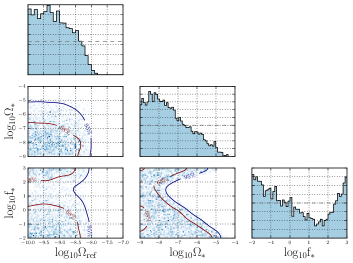
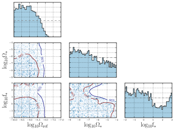
Figure 1: Constraints from LVK O3 data on the broken power-law parameters of a FOPT signal, together with the contribution from the CBC background, assuming dominant bubble collision spectrum (top) and a dominant sound waves spectrum (bottom).

III.1 General broken power-law search

To constrain a GW background from FOPTs, we model the FOPT contribution to the GW spectrum with a broken power-law as

$$\Omega_{\rm bpl}(f)=\Omega_{*}~{}\Big{(}\frac{f}{f_{*}}\Big{)}^{n_{1}}~{}\Bigg{[}1+\Big{(}\frac{f}{f_{*}}\Big{)}^{\Delta}\Bigg{]}^{(n_{2}-n_{1})/\Delta},$$ (12)

where $n_{1}$ and $n_{2}$, respectively, denote the spectral indices before and after the peak, $\Delta$ is a peak smoothing parameter, and $\Omega_{*}$ and $f_{*}$ can be related to the peak amplitude and peak frequency of the spectrum. Note that the spectra introduced in Eqs. (6), (8), approximately follow a broken power-law with parameters $n_{1}=3$, $n_{2}=-1$, $\Delta=4$ and $n_{1}=3$, $n_{2}=-4$, $\Delta=2$ for bubble collisions and sound waves, respectively. We perform a parameter estimation search for both contributions separately, corresponding to the case where one of them dominates the GW spectrum. In each case, the values of $n_{1}$, $n_{2}$, and $\Delta$ are set to the relevant values of that contribution, as given above. Note that in Romero et al. (2021), $n_{2}$ was allowed to vary.

Broken power-law		Phenomenological
$\Omega_{\rm ref}$	LogU[$10^{-10}$, $10^{-7}$]	$\Omega_{\rm ref}$	LogU[$10^{-10}$, $10^{-7}$]
$\Omega_{*}$	LogU[$10^{-9}$, $10^{-4}$]	$\beta/H_{\rm RH}$	LogU[1,$10^{3}$]
$f_{*}$	LogU[$10^{-2}$, $10^{3}$]	$T_{\rm RH}$	LogU[$10^{5}$,$10^{10}$]

Table 1: Summary of the priors used for parameter estimation for the broken power-law model search and the phenomenological model search, where LogU stands for a log-uniform prior. The narrow prior on $\rm\Omega_{ref}$ stems from estimates of the CBC background Abbott et al. (2018). The peak frequency is chosen such that it lies in the region of highest sensitivity in LIGO-Virgo. Values lower than 1 for $\rm\beta/H_{\rm RH}$ are not considered, since otherwise the phase transition would not take place.

The likelihood to perform this search is given by Eq. (10), where $\Omega_{\rm GW}=\Omega_{\rm cbc}+\Omega_{\rm bpl}$. The GW parameters to be constrained are $\mathbf{\theta}_{\rm GW}=(\Omega_{\rm ref},~{}\Omega_{*},~{}f_{*})$ with priors given in Table 1 and results shown in Fig. 1 for bubble collisions (top panel) and sound waves (bottom panel). From the posteriors of the amplitude of the CBC background, $\rm\Omega_{ref}$, upper limits (ULs) at 95% confidence level (CL) are obtained. The value for the case in which bubble collisions dominate is $5.60\times 10^{-9}$, which is consistent with the upper limit obtained in Abbott et al. (2021c); Romero et al. (2021). The UL in the case when sound waves dominate is also consistent with previous searches, with a value $5.70\times 10^{-9}$. Similarly, 95% confidence level contours are obtained on the amplitude and peak frequency of the contribution from FOPTs, $\rm\Omega_{*}$ and $f_{*}$, as depicted in Fig. 1. The values of the Bayes factor are $\log\mathcal{B}^{\rm CBC+BC}_{\rm noise}=-1.26$ and $\log\mathcal{B}^{\rm CBC+SW}_{\rm noise}=-0.80$, showing no evidence for a FOPT signal in the data.

III.2 Phenomenological search

We now proceed with a different model assumption. Instead of the general broken power-law model used above, we consider the GW spectra introduced in Sec. II, more specifically Eqs. (6) and (8), corresponding to bubble collisions and sound waves, respectively. The likelihood used to perform this search is given by Eq. (10), with $\Omega_{\rm GW}=\Omega_{\rm cbc}+\Omega_{\rm bc}$ and $\Omega_{\rm GW}=\Omega_{\rm cbc}+\Omega_{\rm sw}$ for bubble collisions and sounds waves, respectively. Therefore, the GW parameters to be constrained in this search are $\mathbf{\theta}_{\rm GW}=(\Omega_{\rm ref},~{}\beta/H_{\rm RH},~{}T_{\rm RH})$. We again highlight the difference with the search conducted in Romero et al. (2021), where the $\alpha$ parameter was included. As discussed earlier, for supercooled FOPTs, for which $\alpha\gg 1$, neglecting this parameter is a valid assumption. The priors on the parameters used for parameter estimation are given in Table 1, and the resulting posterior distributions are presented in Fig. 2. From the posteriors of the amplitude of the CBC background, $\rm\Omega_{ref}$, ULs at 95% CL are obtained. The value for the case in which bubble collisions or sound waves dominate is $5.89\times 10^{-9}$ and $5.93\times 10^{-9}$, respectively. They are consistent with the upper limit obtained in Abbott et al. (2021c); Romero et al. (2021). Furthermore, exclusions at 95% CL for temperatures $T_{\rm RH}$ and inverse duration of the FOPT $\beta/H_{\rm RH}$ are depicted in Fig. 2.

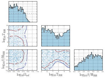
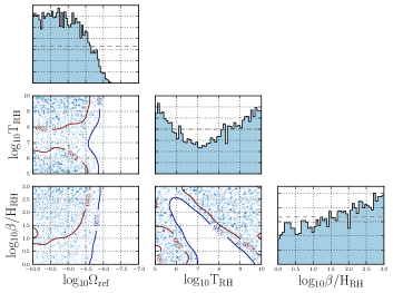
Figure 2: Constraints from LVK O3 data on the phenomenological parameters $\beta/H_{\rm RH}$ and $T_{\rm RH}$ of a supercooled FOPT signal, together with the contribution from the CBC background, assuming a dominant bubble collision spectrum (top) and a dominant sound waves spectrum (bottom).

Let us emphasise that the constraints derived above can be used in any model exhibiting supercooling. More precisely, once a model and its parameters are specified, one can compute the expected FOPT parameters $\beta/H_{\rm RH}$ and $T_{\rm RH}$ (or equivalently $\Omega_{*}$ and $f_{*}$) and compare them with the 95% confidence UL provided here. In this way, one uses GW data to exclude regions of the parameter space in concrete particle physics models. We will illustrate this in the next section for two particle physics models.

IV Two well-motivated particle physics models

The phenomenon of supercooling occurs in theories with Coleman-Weinberg-type symmetry breaking Coleman and Weinberg (1973) or strong coupling. Several models of this type have been investigated in the literature in light of their enhanced GW signals Ellis et al. (2019); Delle Rose et al. (2020); Marzo et al. (2019); Jinno and Takimoto (2017); Lewicki and Vaskonen (2021); Agashe et al. (2020); Von Harling et al. (2020); Ellis et al. (2020a); Lewicki et al. (2021); Prokopec et al. (2019); Jinno et al. (2019); Baratella et al. (2019); Ellis et al. (2020b). In this study, we focus on Model I Ellis et al. (2019) and Model II Delle Rose et al. (2020), which exhibit approximate conformal symmetry. They are both well-motivated from a particle physics point of view and have a minimal particle content. We note, however, that our analysis can be applied to any other model with supercooling. The general goal is to assess the detectability of signals from supercooled FOPTs with the LVK detectors, and determine the regions of parameter space that can be excluded with current GW data.

IV.1 Model I

IV.1.1 Theoretical framework

The first model we consider is based on a theoretically attractive minimal ${\rm U}(1)_{B-L}$ extension of the SM gauge group Marzo et al. (2019); Ellis et al. (2019, 2020b). Upon introducing three right-handed neutrinos, the theory is anomaly-free, realises the seesaw mechanism, and can be incorporated into ${\rm SO}(10)$ grand unification. The model includes only two new bosonic fields: a real scalar $\phi$ and a gauge boson $Z^{\prime}$.

The zero temperature scalar potential is given by

$$V_{0}(\phi)=\frac{1}{4}{\lambda_{\phi}}\phi^{4}$$ (13)

$$+ \sum_{i=\phi,G,Z^{\prime}}\frac{n_{i}}{64\pi^{2}}\left\{m_{i}^{4}(\phi)\left[\log\left(\frac{m_{i}^{2}(\phi)}{\mu^{2}}\right)-c_{i}\right]\right\}\ ,\ \ \ \ \$$

where $n_{i}$ is the number of degrees of freedom, $c_{\phi,G}=3/2$, $c_{Z^{\prime}}=5/6$, $\mu$ is the renormalization scale, and $G$ denotes the Goldstone boson. The field-dependent masses are:

$$m_{Z^{\prime}}^{2}(\phi)=4g^{2}\phi^{2}\ ,\ \ \ \ m_{\phi}^{2}(\phi)=3\lambda_{\phi}\phi^{2}\ ,$$

$$m_{G}^{2}(\phi)=\lambda_{\phi}\phi^{2}\ ,$$ (14)

where $g$ is the gauge coupling. The finite temperature part of the effective potential is

$$V_{\rm T}(\phi,T)$$ (15)

$$= \ \frac{T^{4}}{2\pi^{2}}\sum_{i=\phi,G,Z^{\prime}}\!n_{i}\!\int_{0}^{\infty}\!\!dy\,y^{2}\log\left(1-e^{-\sqrt{m_{i}^{2}(\phi)/T^{2}+y^{2}}}\right)$$

$$+ \ \frac{T}{12\pi}\sum_{j=\phi,G,Z_{L}^{\prime}}\!n^{\prime}_{j}\,\Big{\{}m_{j}^{3}(\phi)-[m_{j}^{2}(\phi)+\Pi_{j}(T)]^{\frac{3}{2}}\Big{\}},$$

with the thermal masses given by

$$\Pi_{\phi}(T)=\Pi_{G}(T)=\left(g^{2}+\tfrac{1}{3}\lambda_{\phi}\right)T^{2}\ ,$$

$$\Pi_{Z^{\prime}_{L}}(T)=4g^{2}T^{2}\ ,$$ (16)

where the subscript $L$ denotes longitudinal components.

This model has only two free parameters relevant for the GW signal: the vacuum expectation value $v$ of the scalar field $\phi$, and the ${\rm U}(1)_{B-L}$ gauge coupling $g$. Trading $v$ for the the gauge boson mass $m_{Z^{\prime}}$, related via

$$m_{Z^{\prime}}={2gv}\ ,$$ (17)

the two parameters describing Model I are $(m_{Z^{\prime}},g)$.

IV.1.2 Constraints from LVK O1+O2+O3 data

For each point $(m_{Z^{\prime}},g)$ of the parameter space, one can compute the parameters describing the phase transition, i.e., $T_{\rm RH}$ and $\beta/H_{\rm RH}$, and the resulting GW spectrum. We restrict ourselves to $m_{Z^{\prime}}\in[10^{4},~{}10^{11}]$ GeV and $g\in[0.3,~{}0.4]$, which corresponds to FOPTs where the GW signal is dominated by sound waves and, therefore, given by Eq. (8) Ellis et al. (2020b). If the gauge coupling $g$ is chosen to be larger than 0.4, the FOPT is not supercooled and $\alpha\sim 1$. Furthermore, we are not exploring values of $g$ below 0.3, as these correspond to a regime where both bubble collisions and sound waves contribute considerably to the GW spectrum, as discussed in Ellis et al. (2020b).

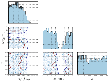
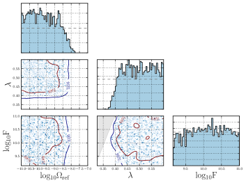
Figure 3: Constraints on the parameter space $(m_{Z^{\prime}},g)$ for Model I (top panel) and on the parameters $\lambda$ and $F$ for Model II (bottom panel), together with constraints on the astrophysical CBC background amplitude $\Omega_{\rm ref}$ using LVK O3 data. The gray region in the bottom plot corresponds to a region where nucleation does not occur and the phase transition does not complete.

Model I		Model II
$\Omega_{\rm ref}$	LogU[$10^{-10}$, $10^{-7}$]	$\Omega_{\rm ref}$	LogU[$10^{-10}$, $10^{-7}$]
$m_{Z^{\prime}}$	LogU[$10^{4}$, $10^{11}$] (GeV)	$F$	LogU[$1.4$$\times$$10^{9}$, $10^{11}$] (GeV)
$g$	U[0.3, 0.4]	$\lambda$	U[$0.325$, $0.6$]

Table 2: Summary of the priors used for parameter estimation for Model I and Model II, where U stands for a uniform and LogU for a log-uniform prior. The narrow prior on $\rm\Omega_{ref}$ stems from estimates of the CBC background Abbott et al. (2018).

We perform a parameter estimation search over this parameter space, and include the contribution of the CBC background. The likelihood is given by Eq. (10), with $\Omega_{\rm GW}=\Omega_{\rm cbc}+\Omega_{\rm sw}$, where $\Omega_{\rm sw}$ is calculated from Eq. (8) using the model parameters $(m_{Z^{\prime}},g)$. Thus, the parameters of the search are $\mathbf{\theta}_{\rm GW}=(\Omega_{\rm ref},~{}m_{Z^{\prime}},~{}g)$. The priors are summarised in Table 2 and the results are shown in Fig. 3 (upper panel) which depicts the resulting posteriors. The upper limits on the amplitude of the astrophysical CBC background are consistent with Abbott et al. (2021c); Romero et al. (2021). Furthermore, a region of parameter space around $m_{Z^{\prime}}\sim\mathcal{O}(10^{8}\text{ GeV})$ is excluded, and corresponds to FOPT GW signals peaked within the frequency range of the LVK detectors.

We now compare the exclusion regions obtained directly on the parameters of the model with the ones deduced from the analysis in Sec. III . Given a choice of the parameters $(m_{Z^{\prime}},g)$, one can verify whether the corresponding values of $(\beta/H_{\rm{RH}},T_{\rm{RH}})$ or $(f_{*},\Omega_{*})$ are excluded using the search analysis in Sec. III. As Fig. 4 demonstrates, a good agreement is found between the various exclusion regions, regardless of the search performed. Therefore, the results obtained in Sec. III are easily reinterpreted in any specific model with supercooling. This is also supported by the analysis we perform below for another well-motivated particle physics model.

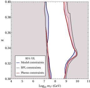
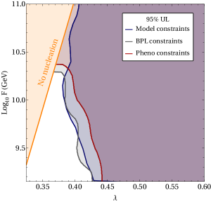
Figure 4: Comparison of the constraints on the parameter space $(m_{Z^{\prime}},g)$ for Model I (top panel) and on $(\lambda,F)$ for Model II (bottom panel) obtained by constraining the model parameters directly as in Fig. 3 (blue line), with those obtained by adopting the BPL model as given in Fig. 1 (gray line), and those adopting the phenomenological model in Fig. 2 (red line).

IV.2 Model II

IV.2.1 Theoretical framework

This model is based on a radiatively broken ${\rm U(1)}$ Peccei-Quinn symmetry Delle Rose et al. (2020), introduced to solve the strong CP problem, and leading to the appearance of a dark matter candidate – the axion. It extends the SM by including just two new complex scalar fields, $S$ and $X$, which are SM singlets, and both carry Peccei-Quinn charges.

The tree-level scalar potential is

$$V_{\rm tree}=\lambda_{S}|S|^{4}+\lambda_{X}|X|^{4}+\lambda_{SX}|S|^{2}|X|^{2}\ .$$ (18)

It exhibits a flat direction for $\lambda_{SX}=-2\sqrt{\lambda_{S}\lambda_{X}}$, which can be parameterised by

$$(S,X)=(\sin\alpha,\cos\alpha)\frac{\sigma}{\sqrt{2}}\ ,\hskip 5.69054pt\sin^{2}\!\alpha=\frac{\sqrt{\lambda_{X}}}{\sqrt{\lambda_{S}}+\sqrt{\lambda_{X}}}\ .\ \ \ \ \ \$$ (19)

The mass of the field along the direction orthogonal to $\sigma$ is

$$m_{\tau}=(4\lambda_{S}\lambda_{X})^{1/4}\sigma\ .$$ (20)

Assuming that the condition for the flat direction holds at the renormalisation scale $\Lambda$, and switching the parameter $\Lambda$ for the field value at the minimum of the potential $F$, the zero temperature scalar potential is given by

$$V_{0}(\sigma)=\frac{2\lambda_{S}\lambda_{X}}{16\pi^{2}}\sigma^{4}\left(\log\frac{\sigma}{F}-\frac{1}{4}\right)\ .$$ (21)

At the minimum $\sigma$ has a loop-suppressed mass, whereas the phase of $X$ is massless up to QCD anomalies, and becomes the axion with a decay constant $F_{a}=F\cos\alpha$. The finite temperature part of the effective potential is given by a formula analogous to Eq. (15), but with just a single term involving $m_{\tau}$. To prevent the finite temperature effects from moving the true vacuum away from the flat direction, we set

$$\lambda_{X}=\lambda_{S}\equiv\lambda\ ,$$ (22)

which is equivalent to imposing a $\mathbb{Z}_{2}$ symmetry at the level of the Lagrangian. As a result, Model II is described by just two parameters: $(\lambda,F)$.

IV.2.2 Constraints from LVK O1+O2+O3 data

Similarly as for Model I, one can compute the FOPT parameters $\beta/H_{\rm{RH}}$ and $T_{\rm{RH}}$, and determine the GW spectrum. The ranges of parameters we consider are: $F\in[1.4\times 10^{9},~{}10^{11}]$ GeV and $\lambda\in[0.325,0.6]$. A value of $F$ smaller than $1.4\times 10^{9}$ GeV (corresponding to an axion decay constant of $10^{9}$ GeV) is experimentally excluded Di Luzio et al. (2020), whereas values of $\lambda$ lower than 0.325 correspond to cases when the phase transition does not complete, i.e., no nucleation occurs. The upper limits on $F$ and $\lambda$ are not constrained and were set arbitrarily in Fig. 4.

We again conduct a parameter estimation directly on the parameters of the model. In the case of Model 2 the dominant GW contribution comes from bubble collisions Delle Rose et al. (2020). In the likelihood given by Eq. (10), $\Omega_{\rm GW}=\Omega_{\rm cbc}+\Omega_{\rm bc}$, where $\Omega_{\rm bc}$ is given by Eq. (6) and can be obtained from the underlying model parameters $(\lambda,F)$. The parameters used for the search are $\mathbf{\theta}_{\rm GW}=(\Omega_{\rm ref},~{}F,~{}\lambda)$ and the priors on $\Omega_{\rm ref}$, $F$ and $\lambda$ are summarised in Table 2. The lower panel in Fig. 3 displays the exclusion regions implied by the current LVK O3 data. The gray region represents part of the parameter space where no nucleation occurs and the phase transition does not complete. As shown in Fig. 3, part of the parameter space can be excluded at a 95% confidence level. This mostly puts constraints on the values of $\lambda$, excluding smaller values, as these are the ones that give rise to the strongest GW signals. Furthermore, one notes consistency with the usual CBC upper limits found in this work, and in Abbott et al. (2021c); Romero et al. (2021).

One can now compare the exclusion regions obtained directly on the model parameters, with those derived following the analysis in Sec. III. The results are shown in Fig. 4, where we note an agreement between the exclusion regions arising from the different searches, similar to the agreement obtained in the case of Model I. Once again, this illustrates how the exclusion regions in Sec. III can be used to constrain any supercooled FOPT at a particle physics model level.

V Detectability of a gravitational-wave background

In this section we briefly compare various ways to address the detectability of a GW background. Instead of using the full Bayesian inference run, one often uses power-law integrated (PI) sensitivity curves, proposed in Thrane and Romano (2013) as a graphical way to address the detectability of a GW background with a power-law dependence within the frequency band of the detector. However, a GW background coming from FOPTs with spectra given in Sec. II would display a broken power-law behaviour. In addition, the presence of the CBC background should be taken into account properly when assessing the experimental sensitivity to cosmological GW backgrounds. In order to quantify the impact of these aspects, we investigate below the applicability of the PI curves method to FOPTs. [We refer the reader to the Appendix for a review of the construction of PI curves, as outlined in Thrane and Romano (2013).]

We now discuss the FOPT detectability with the LVK detectors. Using the broken power-law model described in Sec. III, we generate a GW background signal dominated by bubble collisions for a range of $\Omega_{*},f_{*}$. If a resulting GW background signal is larger than a PI curve constructed, we consider this a detection at the curve’s $\rho_{\rm thr}$ level. In addition, the SNR of each generated GW background signal is calculated. We compare these results to a Bayesian analysis. Again, assuming a domination of bubble collisions, 800 simulated signals over a range of $\Omega_{*},f_{*}$ are injected assuming a combined FOPT+CBC background model with a CBC background amplitude at the reference frequency of $\Omega_{\rm{ref}}=5.9\times 10^{-9}$  Romero et al. (2021). We analyse assuming a pure CBC background, a FOPT signal and a combined FOPT+CBC signal. We subtract the CBC model Bayes factor from the FOPT+CBC Bayes factor to see the preference for the latter model over the former. This procedure is repeated assuming a signal dominated by sound waves, and our results are plotted in Fig. 5.

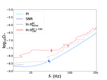
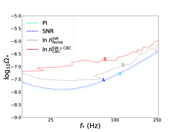
Figure 5: Detectability region within the broken power-law parameter space using PI, SNR curves (dashed) and Bayesian runs (solid) assuming bubble collisions (top) and sound waves (bottom). We choose as detection threshold SNR = 4 and $\ln\mathcal{B}_{\rm{Noise}}^{\rm{FOPT}}=\ln\mathcal{B}_{\rm{CBC}}^{\rm{FOPT+CBC}}=8$.

The calculated PI, SNR and Bayes factor curves follow similar trends. LVK detection capabilities improve for smaller $f_{*}$ and optimise at about 25 Hz, before increasing again. This is explained by the LVK network being most sensitive at this frequency, allowing a more optimistic outlook on broken power-law FOPT signals peaking at this frequency. The PI and SNR detection curves track each other very closely with the SNR curve being slightly more conservative. For values of $f_{*}\leq 250$ Hz, using the PI method one can expect a detection at $\rho_{\rm thr}\geq 4$ for a bubble collision GW background with $\log_{10}\Omega_{*}\geq-6.54$ and $\log_{10}\Omega_{*}\geq-6.44$ for a sound wave GW background. Similarly, one can achieve $\rm{SNR}_{\rm{thr}}\geq 4$ for a bubble collision background with $\log_{10}\Omega_{*}\geq-6.50$, and $\log_{10}\Omega_{*}\geq-6.39$ for a sound wave background. The SNR, PI curves are optimised with $\log_{10}\Omega_{*}\geq-8.70,-8.75$ for a bubble collision dominated background, and $\log_{10}\Omega_{*}\geq-7.89,-7.95$ for a sound wave dominated background when $f_{*}=25$ Hz.

Turning to the Bayesian analysis, we see that the resulting detection curves are more conservative than the PI and SNR ones. For a detection at Bayes factor $\ln\mathcal{B}_{\rm{Noise}}^{\rm{FOPT}}\geq 8$, a bubble collision GW background with $\log_{10}\Omega_{*}\geq-6.32$ and $\log_{10}\Omega_{*}\geq-6.23$ for a sound wave GW background is needed. To find a preference for a combined FOPT+CBC model over a CBC background model at Bayes factor $\ln\mathcal{B}_{\rm{CBC}}^{\rm{FOPT+CBC}}\geq 8$, a bubble collision GW background with $\log_{10}\Omega_{*}\geq-6.28$ and $\log_{10}\Omega_{*}\geq-5.98$ for a sound wave GW background is needed. Similar to the PI, SNR curves, the Bayes factor curves in both FOPT models are optimised when considering models with smaller $f_{*}$. A stronger GW background signal is needed to find a preference for a combined FOPT+CBC model over a pure CBC background.

We conclude that a data-based Bayesian search for broken power-law signal, including the effect of the CBC background, has approximately one order of magnitude less sensitivity in $\Omega_{*}$ than the simple PI estimate, on the frequency range accessible to LVK.

VI Future outlook

We complete our study by looking ahead and making projections for the sensitivity of 3G interferometers to a supercooled FOPT that could have occurred at energies inaccessible to particle colliders. The proposed Einstein Telescope (ET) Punturo et al. (2010) and Cosmic Explorer (CE) Abbott et al. (2017); Reitze et al. (2019) are expected to extend our astrophysical horizon to distant redshift, revealing the majority of CBCs in the Universe. This will help subtract individual sources and reduce the astrophysical contribution to the GW background, in hope of revealing a cosmological background.

We simulate 400 signals containing the residual CBC background Sachdev et al. (2020) and a bubble collision dominated supercooled phase transition for a range of $\beta/H_{\rm{RH}}$ and $T_{\rm{RH}}$ values. We then compute the log Bayes factor of a CBC+FOPT model to noise, and a CBC model only to noise; subtracting the two determines the preference for the presence of a FOPT signal in the data. The analysis is then repeated for the case of a dominant sound wave contribution to the FOPT signal. The 3G network used places ET at Virgo and two CEs at the Hanford and Livingston locations.

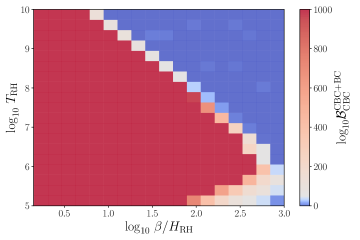
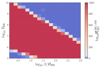
Figure 6: Preference for a model containing a supercooled phase transition and an astrophysical CBC background over a model with an astrophysical background only. Injections of a bubble collision (BC) dominated FOPT show great constraining power of such a signal with a network of 3G detectors (top), and similarly for injections of a sound waves (SW) dominated FOPT (bottom).

Our results are presented in Fig. 6. With the future 3G detectors, we find that a significant part of the parameter space can be probed in both cases. Sound wave and bubble collision dominated supercooled phase transition scenarios are depicted on the top and bottom panels of Fig. 6, respectively.

VII Conclusions

Standard high energy physics experiments are approaching limits of their discovery potential. In many cases, the most natural regions of model parameter space relevant for addressing questions in particle physics are not even within their target sensitivity. New discovery tools are needed to probe physics at the PeV energy scale and beyond. Such a novel and powerful discovery tool has recently been provided by GW detectors, with their relevance destined only to increase in future years, given the upcoming upgrades to existing GW experiments and the construction of new detectors sensitive to a wider range of frequencies.

To demonstrate the huge opportunity for particle physics arising from GW searches, we carried out the pioneering study in which we used the data from the first three LVK observing runs (O1, O2 and O3) to perform a Bayesian analysis and set direct limits on the parameter space of particle physics models. This is a natural extension of the previous work Romero et al. (2021), in which only general constraints on FOPT parameters were derived. In our analysis we focused on supercooled FOPTs, since they are naturally characterised by an enhanced signal strength, potentially already within the reach of current LVK detectors.

To show how the procedure works, we applied our analysis to two well-motivated particle physics models, which address some of the most intriguing open questions about the Universe: the dark matter puzzle, the strong CP problem, the origin of the neutrino masses, and unification of forces. We place the Bayesian 95% upper limits on the parameter space of those models, providing valuable insight into the available room for new physics. The same strategy can be used to impose limits on other models exhibiting supercooled FOPTs and is left for future work.

Apart from conducting the analysis using the available LVK O1-O3 data, we provide an outlook on the reach of 3G detectors. This methodology can also be applied to future LVK upgrades, as well as next generation detectors. It is worth emphasizing that our work bridges the gap between data analysis and phenomenological studies, making the constraints from GW searches easier to reinterpret, and applicable to any particle physics model with a supercooled phase transition.

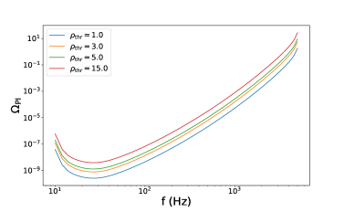
Figure 7: Example of a power-law integrated sensitivity curve for the LVK detectors using O4 sensitivity and assuming a threshold SNR $\rho_{\rm thr}=1,3,5,15$ and an observation time $T=1$ year.

Appendix A Power-law integrated sensitivity curves

We summarise the construction of power-law integrated curves Thrane and Romano (2013). Consider the signal-to-noise ratio (SNR) for a GW background $\Omega_{\rm GW}$ after observing time $T$ by a detector network $M$:

$$\rho=\sqrt{2T}\left[\int_{f_{\rm min}}^{f_{\rm max}}df\frac{\Omega_{\rm GW}^{2}(f)}{\Omega_{\rm eff}^{2}(f)}\right]^{1/2},$$ (23)

where the effective energy density reads

$$\Omega_{\rm eff}(f)=\frac{2\pi^{2}}{3H_{0}^{2}}f^{3}\left[\sum_{I=1}^{M}\sum_{J>I}^{M}\frac{\Gamma_{IJ}^{2}(f)}{P_{nI}(f)P_{nJ}(f)}\right]^{-1/2},$$ (24)

with $\Gamma_{IJ}$ the overlap reduction function and $P_{nI}$ the noise power spectral density of detector $I$. Assuming a power-law spectrum $\Omega_{\rm GW}(f)=\Omega_{\beta}(f/f_{\rm ref})^{\beta}$, one can calculate the value of $\Omega_{\beta}$ such that some SNR threshold $\rho_{\rm thr}$ is reached:

$$\Omega_{\beta}=\frac{\rho_{\rm thr}}{\sqrt{2T}}\left[\int_{f_{\rm min}}^{f_{\rm max}}df\frac{(f/f_{\rm ref})^{2\beta}}{\Omega_{\rm eff}^{2}(f)}\right]^{-1/2}.$$ (25)

This procedure is repeated for a series of $\beta$ values, e.g. $\beta\in\{-10,-9,\dots,9,10\}$. The PI curve is given by:

$$\Omega_{\rm PI}(f)=\max_{\beta}\left[\Omega_{\beta}\left(\frac{f}{f_{\rm ref}}\right)^{\beta}\right].$$ (26)

By construction, any line on a log-scaled plot, corresponding to a power-law GW background, which is tangent to the PI curve, will have an integrated SNR equal to the chosen threshold value $\rho_{\rm thr}$. A curve that falls below the PI curve would be observed with and SNR lower than $\rho_{\rm thr}$, whereas an SNR larger than $\rho_{\rm thr}$ is expected for curves that fall above the PI curve. The result of the above procedure is illustrated in Fig. 7 where the PI curve is shown for the LVK detectors at O4 sensitivity using a threshold SNR of $\rho_{\rm thr}=1,3,5,15$ and assuming an observation time $T=1$ year.

References

- Abbott et al. (2016) B. P. Abbott et al. (LIGO Scientific, Virgo), “Observation of Gravitational Waves from a Binary Black Hole Merger,” Phys. Rev. Lett. 116, 061102 (2016), arXiv:1602.03837 [gr-qc] .
- Abbott et al. (2021a) R. Abbott et al. (LIGO Scientific, VIRGO), “GWTC-2.1: Deep Extended Catalog of Compact Binary Coalescences Observed by LIGO and Virgo During the First Half of the Third Observing Run,” (2021a), arXiv:2108.01045 [gr-qc] .
- Abbott et al. (2021b) R. Abbott et al. (LIGO Scientific, VIRGO, KAGRA), “GWTC-3: Compact Binary Coalescences Observed by LIGO and Virgo During the Second Part of the Third Observing Run,” (2021b), arXiv:2111.03606 [gr-qc] .
- Christensen (2019) Nelson Christensen, “Stochastic Gravitational Wave Backgrounds,” Rept. Prog. Phys. 82, 016903 (2019), arXiv:1811.08797 [gr-qc] .
- Kosowsky et al. (1992) A. Kosowsky, M. S. Turner, and R. Watkins, “Gravitational Radiation from Colliding Vacuum Bubbles,” Phys. Rev. D 45, 4514–4535 (1992).
- Turner (1997) Michael S. Turner, “Detectability of inflation produced gravitational waves,” Phys. Rev. D 55, R435–R439 (1997), arXiv:astro-ph/9607066 .
- Vachaspati and Vilenkin (1985) Tanmay Vachaspati and Alexander Vilenkin, “Gravitational Radiation from Cosmic Strings,” Phys. Rev. D 31, 3052 (1985).
- Sakellariadou (1990) M. Sakellariadou, “Gravitational waves emitted from infinite strings,” Phys. Rev. D 42, 354–360 (1990), [Erratum: Phys.Rev.D 43, 4150 (1991)].
- Hiramatsu et al. (2014) Takashi Hiramatsu, Masahiro Kawasaki, and Ken’ichi Saikawa, “On the estimation of gravitational wave spectrum from cosmic domain walls,” JCAP 02, 031 (2014), arXiv:1309.5001 [astro-ph.CO] .
- Grojean and Servant (2007) C. Grojean and G. Servant, “Gravitational Waves from Phase Transitions at the Electroweak Scale and Beyond,” Phys. Rev. D 75, 043507 (2007), arXiv:hep-ph/0607107 .
- Vaskonen (2017) Ville Vaskonen, “Electroweak baryogenesis and gravitational waves from a real scalar singlet,” Phys. Rev. D 95, 123515 (2017), arXiv:1611.02073 [hep-ph] .
- Dorsch et al. (2017) G. C. Dorsch, S. J. Huber, T. Konstandin, and J. M. No, “A Second Higgs Doublet in the Early Universe: Baryogenesis and Gravitational Waves,” JCAP 05, 052 (2017), arXiv:1611.05874 [hep-ph] .
- Chala et al. (2018) Mikael Chala, Claudius Krause, and Germano Nardini, “Signals of the electroweak phase transition at colliders and gravitational wave observatories,” JHEP 07, 062 (2018), arXiv:1802.02168 [hep-ph] .
- Alves et al. (2019) Alexandre Alves, Tathagata Ghosh, Huai-Ke Guo, Kuver Sinha, and Daniel Vagie, “Collider and Gravitational Wave Complementarity in Exploring the Singlet Extension of the Standard Model,” JHEP 04, 052 (2019), arXiv:1812.09333 [hep-ph] .
- Schwaller (2015) P. Schwaller, “Gravitational Waves from a Dark Phase Transition,” Phys. Rev. Lett. 115, 181101 (2015), arXiv:1504.07263 [hep-ph] .
- Breitbach et al. (2019) Moritz Breitbach, Joachim Kopp, Eric Madge, Toby Opferkuch, and Pedro Schwaller, “Dark, Cold, and Noisy: Constraining Secluded Hidden Sectors with Gravitational Waves,” JCAP 07, 007 (2019), arXiv:1811.11175 [hep-ph] .
- Croon et al. (2018) Djuna Croon, Verónica Sanz, and Graham White, “Model Discrimination in Gravitational Wave spectra from Dark Phase Transitions,” JHEP 08, 203 (2018), arXiv:1806.02332 [hep-ph] .
- Hall et al. (2020) E. Hall, T. Konstandin, R. McGehee, H. Murayama, and G. Servant, “Baryogenesis From a Dark First-Order Phase Transition,” JHEP 04, 042 (2020), arXiv:1910.08068 [hep-ph] .
- Hambye et al. (2018) Thomas Hambye, Alessandro Strumia, and Daniele Teresi, “Super-cool Dark Matter,” JHEP 08, 188 (2018), arXiv:1805.01473 [hep-ph] .
- Baldes and Garcia-Cely (2019) Iason Baldes and Camilo Garcia-Cely, “Strong gravitational radiation from a simple dark matter model,” JHEP 05, 190 (2019), arXiv:1809.01198 [hep-ph] .
- Baldes et al. (2022a) Iason Baldes, Yann Gouttenoire, Filippo Sala, and Géraldine Servant, “Supercool composite Dark Matter beyond 100 TeV,” JHEP 07, 084 (2022a), arXiv:2110.13926 [hep-ph] .
- Azatov et al. (2021a) Aleksandr Azatov, Miguel Vanvlasselaer, and Wen Yin, “Dark Matter production from relativistic bubble walls,” JHEP 03, 288 (2021a), arXiv:2101.05721 [hep-ph] .
- Baldes et al. (2022b) Iason Baldes, Yann Gouttenoire, and Filippo Sala, “Hot and Heavy Dark Matter from Supercooling,” (2022b), arXiv:2207.05096 [hep-ph] .
- Croon et al. (2019) D. Croon, T. E. Gonzalo, and G. White, “Gravitational Waves from a Pati-Salam Phase Transition,” JHEP 02, 083 (2019), arXiv:1812.02747 [hep-ph] .
- Brdar et al. (2019a) V. Brdar, L. Graf, A. J. Helmboldt, and X.-J. Xu, “Gravitational Waves as a Probe of Left-Right Symmetry Breaking,” JCAP 12, 027 (2019a), arXiv:1909.02018 [hep-ph] .
- Huang et al. (2020) Wei-Chih Huang, Francesco Sannino, and Zhi-Wei Wang, “Gravitational Waves from Pati-Salam Dynamics,” Phys. Rev. D 102, 095025 (2020), arXiv:2004.02332 [hep-ph] .
- Okada et al. (2021) Nobuchika Okada, Osamu Seto, and Hikaru Uchida, “Gravitational waves from breaking of an extra in grand unification,” PTEP 2021, 033B01 (2021), arXiv:2006.01406 [hep-ph] .
- Helmboldt et al. (2019) Alexander J. Helmboldt, Jisuke Kubo, and Susan van der Woude, “Observational prospects for gravitational waves from hidden or dark chiral phase transitions,” Phys. Rev. D 100, 055025 (2019), arXiv:1904.07891 [hep-ph] .
- Croon et al. (2020) Djuna Croon, Jessica N. Howard, Seyda Ipek, and Timothy M. P. Tait, “QCD baryogenesis,” Phys. Rev. D 101, 055042 (2020), arXiv:1911.01432 [hep-ph] .
- Huang et al. (2021) Wei-Chih Huang, Manuel Reichert, Francesco Sannino, and Zhi-Wei Wang, “Testing the dark SU(N) Yang-Mills theory confined landscape: From the lattice to gravitational waves,” Phys. Rev. D 104, 035005 (2021), arXiv:2012.11614 [hep-ph] .
- Cheung et al. (2012) Clifford Cheung, Alex Dahlen, and Gilly Elor, “Bubble Baryogenesis,” JHEP 09, 073 (2012), arXiv:1205.3501 [hep-ph] .
- Katz and Riotto (2016) Andrey Katz and Antonio Riotto, “Baryogenesis and Gravitational Waves from Runaway Bubble Collisions,” JCAP 11, 011 (2016), arXiv:1608.00583 [hep-ph] .
- Hasegawa et al. (2019) T. Hasegawa, N. Okada, and O. Seto, “Gravitational Waves from the Minimal Gauged Model,” Phys. Rev. D 99, 095039 (2019), arXiv:1904.03020 [hep-ph] .
- Fornal and Shams Es Haghi (2020) Bartosz Fornal and Barmak Shams Es Haghi, “Baryon and Lepton Number Violation from Gravitational Waves,” Phys. Rev. D 102, 115037 (2020), arXiv:2008.05111 [hep-ph] .
- Baldes et al. (2021) Iason Baldes, Simone Blasi, Alberto Mariotti, Alexander Sevrin, and Kevin Turbang, “Baryogenesis via relativistic bubble expansion,” Phys. Rev. D 104, 115029 (2021), arXiv:2106.15602 [hep-ph] .
- Azatov et al. (2021b) Aleksandr Azatov, Miguel Vanvlasselaer, and Wen Yin, “Baryogenesis via relativistic bubble walls,” JHEP 10, 043 (2021b), arXiv:2106.14913 [hep-ph] .
- Brdar et al. (2019b) V. Brdar, A. J. Helmboldt, and J. Kubo, “Gravitational Waves from First-Order Phase Transitions: LIGO as a Window to Unexplored Seesaw Scales,” JCAP 02, 021 (2019b), arXiv:1810.12306 [hep-ph] .
- Okada and Seto (2018) N. Okada and O. Seto, “Probing the Seesaw Scale with Gravitational Waves,” Phys. Rev. D 98, 063532 (2018), arXiv:1807.00336 [hep-ph] .
- Di Bari et al. (2021) Pasquale Di Bari, Danny Marfatia, and Ye-Ling Zhou, “Gravitational waves from first-order phase transitions in Majoron models of neutrino mass,” JHEP 10, 193 (2021), arXiv:2106.00025 [hep-ph] .
- Zhou et al. (2022) Ruiyu Zhou, Ligong Bian, and Yong Du, “Electroweak Phase Transition and Gravitational Waves in the Type-II Seesaw Model,” (2022), arXiv:2203.01561 [hep-ph] .
- Dev et al. (2019) P. S. B. Dev, F. Ferrer, Y. Zhang, and Y. Zhang, “Gravitational Waves from First-Order Phase Transition in a Simple Axion-Like Particle Model,” JCAP 11, 006 (2019), arXiv:1905.00891 [hep-ph] .
- Von Harling et al. (2020) Benedict Von Harling, Alex Pomarol, Oriol Pujolàs, and Fabrizio Rompineve, “Peccei-Quinn Phase Transition at LIGO,” JHEP 04, 195 (2020), arXiv:1912.07587 [hep-ph] .
- Delle Rose et al. (2020) Luigi Delle Rose, Giuliano Panico, Michele Redi, and Andrea Tesi, “Gravitational Waves from Supercool Axions,” JHEP 04, 025 (2020), arXiv:1912.06139 [hep-ph] .
- Demidov et al. (2018) S. V. Demidov, D. S. Gorbunov, and D. V. Kirpichnikov, “Gravitational Waves from Phase Transition in Split NMSSM,” Phys. Lett. B 779, 191–194 (2018), arXiv:1712.00087 [hep-ph] .
- Craig et al. (2020) Nathaniel Craig, Noam Levi, Alberto Mariotti, and Diego Redigolo, “Ripples in Spacetime from Broken Supersymmetry,” JHEP 21, 184 (2020), arXiv:2011.13949 [hep-ph] .
- Fornal et al. (2021) Bartosz Fornal, Barmak Shams Es Haghi, Jiang-Hao Yu, and Yue Zhao, “Gravitational Waves from Mini-Split SUSY,” Phys. Rev. D 104, 115005 (2021), arXiv:2104.00747 [hep-ph] .
- Greljo et al. (2020) A. Greljo, T. Opferkuch, and B. A. Stefanek, “Gravitational Imprints of Flavor Hierarchies,” Phys. Rev. Lett. 124, 171802 (2020), arXiv:1910.02014 [hep-ph] .
- Fornal (2021) Bartosz Fornal, “Gravitational Wave Signatures of Lepton Universality Violation,” Phys. Rev. D 103, 015018 (2021), arXiv:2006.08802 [hep-ph] .
- Caldwell et al. (2022) Robert Caldwell et al., “Detection of Early-Universe Gravitational Wave Signatures and Fundamental Physics,” (2022), arXiv:2203.07972 [gr-qc] .
- Coleman and Weinberg (1973) Sidney Coleman and Erick Weinberg, “Radiative corrections as the origin of spontaneous symmetry breaking,” Phys. Rev. D 7, 1888–1910 (1973).
- Creminelli et al. (2002) Paolo Creminelli, Alberto Nicolis, and Riccardo Rattazzi, “Holography and the electroweak phase transition,” JHEP 03, 051 (2002), arXiv:hep-th/0107141 .
- Randall and Servant (2007) Lisa Randall and Geraldine Servant, “Gravitational waves from warped spacetime,” JHEP 05, 054 (2007), arXiv:hep-ph/0607158 .
- Nardini et al. (2007) Germano Nardini, Mariano Quiros, and Andrea Wulzer, “A Confining Strong First-Order Electroweak Phase Transition,” JHEP 09, 077 (2007), arXiv:0706.3388 [hep-ph] .
- Konstandin and Servant (2011) Thomas Konstandin and Geraldine Servant, “Cosmological Consequences of Nearly Conformal Dynamics at the TeV scale,” JCAP 12, 009 (2011), arXiv:1104.4791 [hep-ph] .
- Jinno and Takimoto (2017) Ryusuke Jinno and Masahiro Takimoto, “Probing a classically conformal B-L model with gravitational waves,” Phys. Rev. D 95, 015020 (2017), arXiv:1604.05035 [hep-ph] .
- von Harling and Servant (2018) Benedict von Harling and Geraldine Servant, “QCD-induced Electroweak Phase Transition,” JHEP 01, 159 (2018), arXiv:1711.11554 [hep-ph] .
- Baratella et al. (2019) Pietro Baratella, Alex Pomarol, and Fabrizio Rompineve, “The Supercooled Universe,” JHEP 03, 100 (2019), arXiv:1812.06996 [hep-ph] .
- Prokopec et al. (2019) Tomislav Prokopec, Jonas Rezacek, and Bogumiła Świeżewska, “Gravitational waves from conformal symmetry breaking,” JCAP 02, 009 (2019), arXiv:1809.11129 [hep-ph] .
- Marzo et al. (2019) Carlo Marzo, Luca Marzola, and Ville Vaskonen, “Phase transition and vacuum stability in the classically conformal B–L model,” Eur. Phys. J. C 79, 601 (2019), arXiv:1811.11169 [hep-ph] .
- Ellis et al. (2019) John Ellis, Marek Lewicki, José Miguel No, and Ville Vaskonen, “Gravitational wave energy budget in strongly supercooled phase transitions,” JCAP 06, 024 (2019), arXiv:1903.09642 [hep-ph] .
- Jinno et al. (2019) Ryusuke Jinno, Hyeonseok Seong, Masahiro Takimoto, and Choong Min Um, “Gravitational waves from first-order phase transitions: Ultra-supercooled transitions and the fate of relativistic shocks,” JCAP 10, 033 (2019), arXiv:1905.00899 [astro-ph.CO] .
- Lewicki and Vaskonen (2021) Marek Lewicki and Ville Vaskonen, “Gravitational waves from colliding vacuum bubbles in gauge theories,” Eur. Phys. J. C 81, 437 (2021), arXiv:2012.07826 [astro-ph.CO] .
- Agashe et al. (2020) Kaustubh Agashe, Peizhi Du, Majid Ekhterachian, Soubhik Kumar, and Raman Sundrum, “Cosmological Phase Transition of Spontaneous Confinement,” JHEP 05, 086 (2020), arXiv:1910.06238 [hep-ph] .
- Ellis et al. (2020a) John Ellis, Marek Lewicki, and José Miguel No, “Gravitational waves from first-order cosmological phase transitions: lifetime of the sound wave source,” JCAP 07, 050 (2020a), arXiv:2003.07360 [hep-ph] .
- Ellis et al. (2020b) John Ellis, Marek Lewicki, and Ville Vaskonen, “Updated predictions for gravitational waves produced in a strongly supercooled phase transition,” JCAP 11, 020 (2020b), arXiv:2007.15586 [astro-ph.CO] .
- Agashe et al. (2021) Kaustubh Agashe, Peizhi Du, Majid Ekhterachian, Soubhik Kumar, and Raman Sundrum, “Phase Transitions from the Fifth Dimension,” JHEP 02, 051 (2021), arXiv:2010.04083 [hep-th] .
- Lewicki et al. (2021) Marek Lewicki, Oriol Pujolàs, and Ville Vaskonen, “Escape from supercooling with or without bubbles: gravitational wave signatures,” Eur. Phys. J. C 81, 857 (2021), arXiv:2106.09706 [astro-ph.CO] .
- Romero et al. (2021) Alba Romero, Katarina Martinovic, Thomas A. Callister, Huai-Ke Guo, Mario Martinez, Mairi Sakellariadou, Feng-Wei Yang, and Yue Zhao, “Implications for first-order cosmological phase transitions from the third LIGO-Virgo observing run,” Physical Review Letters 126 (2021), 10.1103/physrevlett.126.151301.
- Linde (1983) A. D. Linde, “Decay of the False Vacuum at Finite Temperature,” Nuclear Physics B 216, 421 – 445 (1983).
- Espinosa et al. (2010) J. R. Espinosa, T. Konstandin, J. M. No, and G. Servant, “Energy Budget of Cosmological First-Order Phase Transitions,” JCAP 06, 028 (2010), arXiv:1004.4187 [hep-ph] .
- Caprini et al. (2016) C. Caprini et al., “Science with the Space-Based Interferometer eLISA. II: Gravitational Waves from Cosmological Phase Transitions,” JCAP 04, 001 (2016), arXiv:1512.06239 [astro-ph.CO] .
- Kamionkowski et al. (1994) M. Kamionkowski, A. Kosowsky, and M. S. Turner, “Gravitational Radiation from First Order Phase Transitions,” Phys. Rev. D 49, 2837–2851 (1994), arXiv:astro-ph/9310044 .
- Huber and Konstandin (2008) S. J. Huber and T. Konstandin, “Gravitational Wave Production by Collisions: More Bubbles,” JCAP 09, 022 (2008), arXiv:0806.1828 [hep-ph] .
- Hindmarsh et al. (2014) M. Hindmarsh, S. J. Huber, K. Rummukainen, and D. J. Weir, “Gravitational Waves from the Sound of a First Order Phase Transition,” Phys. Rev. Lett. 112, 041301 (2014), arXiv:1304.2433 [hep-ph] .
- Guo et al. (2021) Huai-Ke Guo, Kuver Sinha, Daniel Vagie, and Graham White, “Phase Transitions in an Expanding Universe: Stochastic Gravitational Waves in Standard and Non-Standard Histories,” JCAP 01, 001 (2021), arXiv:2007.08537 [hep-ph] .
- Abbott et al. (2021c) R. Abbott et al., “Upper limits on the isotropic gravitational-wave background from advanced ligo and advanced virgo’s third observing run,” Phys. Rev. D 104, 022004 (2021c).
- (77) https://dcc.ligo.org/G2001287/public.
- Romano and Cornish (2017) J.D. Romano and N.J. Cornish, “Detection methods for stochastic gravitational-wave backgrounds: a unified treatment,” Liv. Rev. Relativ. 20, 2 (2017).
- Abbott et al. (2018) B. P. Abbott et al. (LIGO Scientific Collaboration and Virgo Collaboration), “Gw170817: Implications for the stochastic gravitational-wave background from compact binary coalescences,” Phys. Rev. Lett. 120, 091101 (2018).
- Di Luzio et al. (2020) Luca Di Luzio, Maurizio Giannotti, Enrico Nardi, and Luca Visinelli, “The landscape of QCD axion models,” Phys. Rept. 870, 1–117 (2020), arXiv:2003.01100 [hep-ph] .
- Thrane and Romano (2013) Eric Thrane and Joseph D. Romano, “Sensitivity curves for searches for gravitational-wave backgrounds,” Physical Review D 88 (2013), 10.1103/physrevd.88.124032.
- Punturo et al. (2010) M. Punturo et al., “The Einstein Telescope: A third-generation gravitational wave observatory,” Class. Quant. Grav. 27, 194002 (2010).
- Abbott et al. (2017) B P Abbott et al., “Exploring the sensitivity of next generation gravitational wave detectors,” Classical and Quantum Gravity 34, 044001 (2017).
- Reitze et al. (2019) David Reitze et al., “The US Program in Ground-Based Gravitational Wave Science: Contribution from the LIGO Laboratory,” Bull. Am. Astron. Soc. 51, 141 (2019), arXiv:1903.04615 [astro-ph.IM] .
- Sachdev et al. (2020) Surabhi Sachdev, Tania Regimbau, and B. S. Sathyaprakash, “Subtracting compact binary foreground sources to reveal primordial gravitational-wave backgrounds,” Phys. Rev. D 102, 024051 (2020), arXiv:2002.05365 [gr-qc] .
- Hunter (2007) J. D. Hunter, “Matplotlib: A 2d graphics environment,” Computing in Science & Engineering 9, 90–95 (2007).
- van der Walt et al. (2011) S. van der Walt, S. C. Colbert, and G. Varoquaux, “The numpy array: A structure for efficient numerical computation,” Computing in Science Engineering 13, 22–30 (2011).
- Ashton et al. (2019) Gregory Ashton et al., “BILBY: A user-friendly Bayesian inference library for gravitational-wave astronomy,” Astrophys. J. Suppl. 241, 27 (2019), arXiv:1811.02042 [astro-ph.IM] .
- Buchner, J. et al. (2014) Buchner, J., Georgakakis, A., Nandra, K., Hsu, L., Rangel, C., Brightman, M., Merloni, A., Salvato, M., Donley, J., and Kocevski, D., “X-ray spectral modelling of the agn obscuring region in the cdfs: Bayesian model selection and catalogue,” A&A 564, A125 (2014).
- Thain et al. (2005) Douglas Thain, Todd Tannenbaum, and Miron Livny, “Distributed computing in practice: the condor experience.” Concurrency - Practice and Experience 17, 323–356 (2005).