Factor Graph Fusion of Raw GNSS Sensing with IMU and Lidar
for Precise Robot Localization without a Base Station

Abstract

Accurate localization is a core component of a robot’s navigation system. To this end, global navigation satellite systems (GNSS) can provide absolute measurements outdoors and, therefore, eliminate long-term drift. However, fusing GNSS data with other sensor data is not trivial, especially when a robot moves between areas with and without sky view. We propose a robust approach that tightly fuses raw GNSS receiver data with inertial measurements and, optionally, lidar observations for precise and smooth mobile robot localization. A factor graph with two types of GNSS factors is proposed. First, factors based on pseudoranges, which allow for global localization on Earth. Second, factors based on carrier phases, which enable highly accurate relative localization, which is useful when other sensing modalities are challenged. Unlike traditional differential GNSS, this approach does not require a connection to a base station. On a public urban driving dataset, our approach achieves accuracy comparable to a state-of-the-art algorithm that fuses visual inertial odometry with GNSS data—despite our approach not using the camera, just inertial and GNSS data. We also demonstrate the robustness of our approach using data from a car and a quadruped robot moving in environments with little sky visibility, such as a forest. The accuracy in the global Earth frame is still $12\text{\,}\mathrm{m}\text{/}$, while the estimated trajectories are discontinuity-free and smooth. We also show how lidar measurements can be tightly integrated. We believe this is the first system that fuses raw GNSS observations (as opposed to fixes) with lidar in a factor graph.

I INTRODUCTION

A key enabler for autonomous navigation is accurate localization using only a robot’s onboard sensors. Effective sensor fusion is essential to maximize information gain from each sensing modality. For example, proprioception based on inertial measurement units (IMUs) or encoders together with exteroception from cameras or lidars can be used to achieve a smooth, but slowly drifting, estimate of the motion of a mobile platform in a local environment. In contrast, satellite navigation can be used to estimate positions in a global Earth frame. These estimates are drift-free, but require sky visibility. Therefore, fusion of satellite navigation, proprioception, and exteroception is desirable for long-term autonomy.

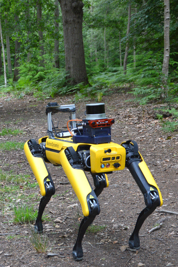
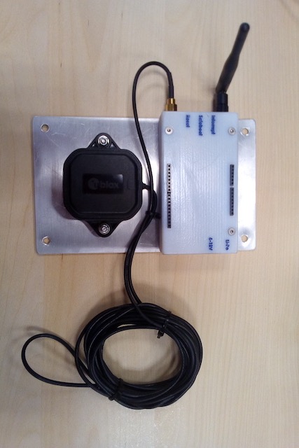
Figure 1: Setups for experimental validation. Left: a car driving on public roads. Center: a quadruped robot moving in urban and forest environments. Right: a GNSS receiver carried handheld. Raw GNSS measurements were tightly fused with inertial sensing and optionally lidar using factor graphs.

The most popular way to fuse data from global navigation satellite systems (GNSS) with onboard perception sensing is two-stage fusion. First, an independent estimator running on the GNSS receiver computes global position fixes from raw GNSS observations. These fixes are then used as position priors within a second-stage pose estimator with proprioceptive and exteroceptive measurements [1, 2]. However, this two-stage fusion has several disadvantages, e.g., the two stages are only loosely coupled, which usually causes lower accuracy and higher uncertainty, especially, when a receiver acquires only a few satellites, or if the internal estimator dynamics of the first stage are unknown. Furthermore, maintaining a persistent network connection for differential GNSS (DGNSS) is impossible or inconvenient in some applications. Without DGNSS, receiver position uncertainty is in the order of several meters. Because of this, GNSS can only be used to anchor a robot’s trajectory in the global Earth frame or to correct long-term drift, but cannot aid accurate local navigation, e.g., if the robot’s exteroception fails.

We follow an alternative approach that addresses these disadvantages by instead fusing the raw observations of the individual satellites with proprioceptive and exteroceptive measurements in a single state estimator, which is more tightly coupled. This allows us to leverage information from even just a few satellites (e.g., less than four)—information which would be discarded in the two-stage approach.

For each visible satellite and a given frequency band, a conventional GNSS receiver can provide three types of observables: pseudoranges, carrier phases, and Doppler shifts. These measurements are affected by a number of errors, rendering fusion particularly challenging and requiring robust optimization. In addition, the different observables have distinct properties: pseudoranges have a comparably high uncertainty while carrier phases are accurate, but challenging to use in real time without a permanent communication link to a base station. Our algorithm addresses both challenges.

Specifically, the contributions of our work are:

• A novel factor graph design incorporating two types of raw GNSS observables (pseudroanges for drift-free localization in the global Earth frame and differential carrier phases for accurate and smooth local positioning) together with inertial measurements and optionally lidar—to our knowledge the first factor graph design to do so.

• A single real-time optimization phase, which implicitly handles GNSS initialization, normal operation, and GNSS drop-out. This eliminates the need to switch between different modes for the aforementioned phases and leads to fast convergence.

• An extensive evaluation on a car and a quadruped robot moving in challenging scenarios and comparison against the state-of-the-art on a public dataset.

II RELATED WORK

Fusion of individual GNSS satellite observations (rather than pre-computed GNSS fixes) with proprioceptive and exteroceptive measurements in a single estimation framework has been pursued in previous work. Traditional methods for integration of GNSS and proprioception, e.g, inertial or encoder measurements, often used filter-based estimation [3, 4]. In contrast, some recent approaches from the robotics community leveraged factor graph optimization. Factor graphs are a popular estimation framework for various fusion problems in robotics [5] and it would be desirable to be able to incorporate raw GNSS observations in this manner. Most approaches used the pseudoranges provided by the GNSS receiver [6, 7, 8, 9, 10, 11, 12]. A pseudorange is the observed travel time of a radio signal from a satellite to the receiver multiplied by the speed of light. They can be seen as range-only observations of distant landmarks; although, pseudoranges usually have much larger meter-scale uncertainties than the centimeter-scale ones of visual landmarks [12]. For example, Gong et al., Wen et al., and Cao et al. fused pseudoranges with combinations of visual or inertial measurements to show that a tightly coupled approach can be robust in urban canyon scenarios with limited sky visibility [12, 8, 13]. They achieved mean positioning errors of a few meters. Due to their meter-scale measurement uncertainty, pseudoranges cannot be employed for centimeter-accurate localization—only for anchoring a trajectory in a global Earth frame and eliminating odometry drift. For accurate local navigation, these approaches rely on a combination of proprioception and exteroception.

To overcome this limitation, carrier-phase observations can also be used. The satellites transmit their data on carrier signals in the gigahertz range, i.e., sine waves with fixed frequencies. If the receiver could measure the number of sine-wave periods between the satellite and itself, this would serve as an additional observation that is proportional to the receiver-satellite distance. It would be more accurate than the pseudorange because signal wavelengths are in the range $1826\text{\,}\mathrm{cm}\text{/}$. However, the receiver cannot count the absolute number of sine-wave periods. Instead, it can observe the phase of the carrier wave and count the change in the number of waves since the receiver first locked onto the signal. (The sum of these values is usually referred to as the carrier phase.) Thus, the range observation can only be inferred up to an unknown integer number of wavelengths, known as the integer ambiguity, which is the number of full waves when the signal was locked. Usually, real-time kinematic positioning (RTK) is used to resolve the integer ambiguity in real time. However, this requires a persistent connection between the moving GNSS receiver (the rover) and a nearby stationary second receiver at a known location (the base).

In the literature, approaches have been described that could make use of carrier phases in real time without the need for a base station. For example, Suzuki used carrier phases to create factors between states at different times to obtain relative distance measurements w.r.t. past epochs [14]. The author named this method time-relative RTK because of its similarity to RTK—with the current observations as rover observations and a set of previous observations as observations to a virtual base station. For each continuously tracked satellite, the approach estimated the integer ambiguity using the LAMBDA method [15, 16]. If the method could not resolve the integer ambiguity, then no factor was added to the graph. In this way, the integer ambiguity estimation was not tightly coupled with the factor-graph-based state estimation. Combining these carrier-phase factors with pseudorange and Doppler-shift factors in a single factor graph, Suzuki achieved mean positioning errors of $25\text{\,}\mathrm{cm}\text{/}$ after UAV flights over $200\text{\,}\mathrm{m}\text{/}$ or $100\text{\,}\mathrm{s}\text{/}$ with good sky visibility and post-processing of data from a single-frequency receiver. There was no real-time evaluation of this method and it did not address fusion with non-GNSS measurements.

Lee et al. described a second method called sequential-differential GNSS in which they also create differential carrier-phase factors between different states in time [17]. This approach also canceled the integer ambiguities. It fused the carrier phases with pseudorange, Doppler shift, visual, and inertial measurements in a multi-state constraint Kalman filter (MSCKF). However, they also used time-relative factors for the pseudoranges. They anchored the local trajectory in the global Earth frame during an initialization phase and afterwards only used the pseudorange and carrier-phase observations for relative localization w.r.t. previously estimated states. This limits the usefulness of pseudorange observations for reducing long-term drift, especially, if sky visibility is lost intermittently or very limited. They demonstrated an RMSE of $0.32\text{\,}\mathrm{m}\text{/}$ on a handheld dataset where sky visibility was never interrupted and differential GNSS factors could always be created between the current and previous state.

In summary, no method has been presented yet that tightly fuses pseudoranges and carrier phases with proprioception and/or exteroception for long-term autonomous localization in real time using a single GNSS receiver. Furthermore, to the best of our knowledge, tight factor graph fusion of raw GNSS data with lidar has not been addressed in the literature.

III PROBLEM STATEMENT

We aim to estimate the pose of a mobile platform that is equipped with a GNSS receiver, an IMU, and optionally a lidar—in real time and in a global Earth frame. The estimated trajectory is required to be smooth/discontinuity-free.

III-A Frames

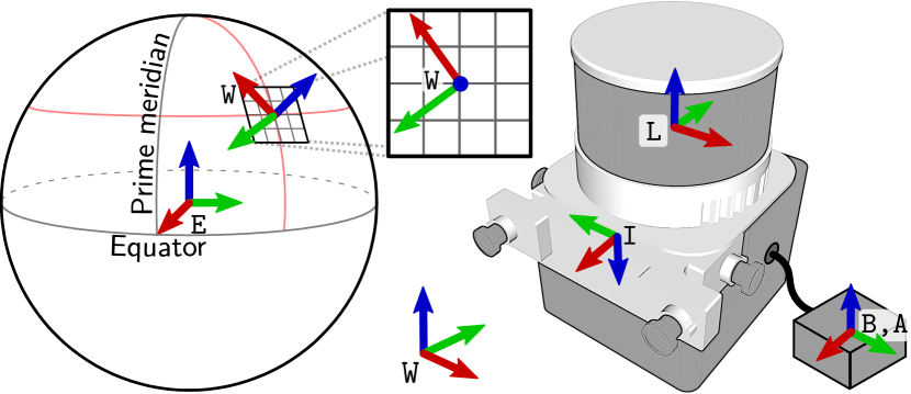
Figure 2: Reference frames: the Earth-centered-Earth-fixed (ECEF) frame $\mathtt{E}$, the local frame $\mathtt{W}$, and the frames on the platforms, including base $\mathtt{{B}}$, which coincides with the GNSS antenna frame $\mathtt{{A}}$, IMU frame $\mathtt{I}$, and lidar frame $\mathtt{L}$.

Ultimately, we are interested in position estimates in geographic coordinates (latitude, longitude). However, for computational reasons, we internally use the Cartesian Earth-centered-Earth-fixed (ECEF) frame $\mathtt{E}$ as global frame. Its $z$-axis is the Earth’s rotation axis, and its $x$-axis points to the prime meridian, cf. Fig. 2.

If the system has exteroceptive sensors, then we are not only interested in a global position estimate, but also in maintaining a smooth local trajectory with no discontinuities during initial GNSS convergence. Therefore, we establish a local frame $\mathtt{W}$ that we align with the platform’s pose at the start of the experiment. We estimate the transformation $\mathbf{T}_{\mathtt{E}\mathtt{W}}\in\mathrm{SO}(3)\times\mathbb{R}^{3}$ between local frame $\mathtt{W}$ and global frame $\mathtt{E}$ jointly with the platform position in frame $\mathtt{W}$. This ensures that the position estimate in $\mathtt{W}$ remains smooth even in scenarios where $\mathbf{T}_{\mathtt{E}\mathtt{W}}$ converges slowly due to no or little GNSS observations being available at the start of an experiment.

If the sensing system has only GNSS and inertial sensing, then we set $\mathtt{W}$ to be identical to $\mathtt{E}$. The frames rigidly attached to the robot are base $\mathtt{{B}}$ (coincident with the GNSS antenna frame $\mathtt{{A}}$), IMU $\mathtt{I}$, and lidar $\mathtt{L}$, see Fig. 2.

III-B State

The state of the system at time $t_{i}$ is

$$\boldsymbol{x}_{i}\triangleq\left[\mathbf{R}_{i},\mathbf{p}_{i},\mathbf{v}_{i},\mathbf{b}^{\mathrm{g}}_{i}\,\;\mathbf{b}^{\mathrm{a}}_{i},\delta\mathbf{t}^{\mathrm{r}}_{i}\right]\in\mathrm{SO}(3)\times\mathbb{R}^{12+M},$$ (1)

where $\mathbf{R}_{i}=\mathbf{R}_{\mathtt{{W}}\mathtt{{B}}}(t_{i})\in\mathrm{SO}(3)$ and $\mathbf{p}_{i}=\tensor[_{\mathtt{{W}}}]{\mathbf{p}}{{}_{\mathtt{{W}}\mathtt{{B}}}}(t_{i})\in\mathbb{R}^{3}$ are the orientation and position of the base $\mathtt{{B}}$ with respect to $\mathtt{{W}}$, respectively; $\mathbf{v}_{i}=\tensor[_{\mathtt{{B}}}]{\mathbf{v}}{{}_{\mathtt{{W}}\mathtt{{B}}}}(t_{i})\in\mathbb{R}^{3}$ is the linear velocity of $\mathtt{{B}}$ with respect to $\mathtt{W}$ expressed in $\mathtt{{B}}$. The IMU’s slowly changing gyroscope and accelerometer biases $\mathbf{b}^{\mathrm{g}}_{i},\mathbf{b}^{\mathrm{a}}_{i}\in\mathbb{R}^{3}$ are expressed in frame $\mathtt{{I}}$. Finally, $\delta\mathbf{t}^{\mathrm{r}}_{i}\in\mathbb{R}^{M}$ is the vector of the clock offsets between each satellite system and the receiver clock. Our receiver accesses four satellite systems (i.e., $M=4$): GPS, BeiDou, GLONASS, and Galileo.

If the setup includes a lidar, we estimate the transformation $\mathbf{T}_{\mathtt{E}\mathtt{W}}$ in addition to the system states $\boldsymbol{x}_{i}$. The history of all unknowns is then

$$\mathcal{X}_{k}\triangleq\left\{\left\{\boldsymbol{x}_{i}\right\}_{i\in{\cal T}_{k}},\mathbf{T}_{\mathtt{E}\mathtt{W}}\right\},$$ (2)

where ${\cal T}_{k}$ is the set of all state indices in a fixed-length time window up to time $t_{k}$.

III-C Measurements

The measurements include the proper acceleration and angular velocity in the IMU frame $\mathtt{I}$ and lidar point clouds ${\cal L}_{ij}$. Inertial measurements are received as a set between times $t_{i}$ and $t_{j}$ as ${\cal I}_{ij}$. They are preintegrated after gravity/bias compensation, as explained in Sec. IV-A. The GNSS receiver observes pseudoranges ${\cal P}_{i}$ and double-differenced carrier phases ${\cal C}_{ij}$. (The latter are explained in Sec. IV-D.) Thus, all measurements in a time window ${\cal T}_{k}$ are

$$\mathcal{Z}_{k}\triangleq\left\{{\cal I}_{ij},{\cal L}_{ij},{\cal P}_{i},{\cal C}_{ij}\right\}_{i,j\in{\cal T}_{k}}.$$ (3)

We create a state $\boldsymbol{x}_{i}$ whenever there is a GNSS observation at time $t_{i}$ and motion correct a potentially received lidar point cloud at that timestamp [18]. If there is no GNSS observation for a certain amount of time, e.g., due to no sky visibility, we create a state with lidar and inertial measurements only.

III-D Maximum-a-Posteriori Estimation

We maximize the likelihood of the measurements ${\cal Z}_{k}$, given the history of states ${\cal X}_{k}$

$$\mathcal{X}^{*}_{k}=\operatorname*{arg\,max}_{\mathcal{X}_{k}}p(\mathcal{X}_{k}|\mathcal{Z}_{k})\propto p(\mathcal{X}_{0})p(\mathcal{Z}_{k}|\mathcal{X}_{k}),$$ (4)

where measurements are assumed to be conditionally independent and corrupted by white Gaussian noise. Therefore, we can express Eq. (4) as a least-squares minimization [5]

$$\begin{split}\mathcal{X}^{*}_{k}=\operatorname*{arg\,min}_{\mathcal{X}_{k}}&\|\mathbf{r}_{0}\|^{2}_{\Sigma_{0}}\\ +\sum_{i,j\in{\cal T}_{k}}\bigg{(}&\|\mathbf{r}_{{\cal I}_{ij}}\|^{2}_{\Sigma_{{\cal I}_{ij}}}+\|\mathbf{r}_{{\cal L}_{ij}}\|^{2}_{\Sigma_{{\cal L}_{ij}}}\\ +\sum_{\rho_{i}^{m}\in{\cal P}_{i}}&\|r_{\rho_{i}^{m}}\|^{2}_{\sigma_{\rho_{i}^{m}}}+\sum_{\Delta\Delta\phi^{mn}_{ij}\in{\cal C}_{ij}}\|r_{\Delta\Delta\phi^{mn}_{ij}}\|^{2}_{\sigma_{\Delta\Delta\phi^{mn}_{ij}}}\bigg{)},\end{split}$$ (5)

where ${\cal T}_{k}$ is the set of all state indices in the sliding smoothing window up to time $t_{k}$. Each term is the residual associated with a factor type, weighted by the inverse of its covariance matrix. Residuals include a prior, IMU factors, relative odometry factors from lidar, and two types of GNSS factors, which are detailed in the following section.

IV FACTOR GRAPH FORMULATION

Figure 3: Factor graph structure with variable nodes (large circles) for states $\boldsymbol{x}_{i}$ and transformation $\mathbf{T}_{\mathtt{E}\mathtt{W}}$ between local frame and global Earth frame and factor nodes (small, colored) for priors, and properioceptive (IMU), exteroceptive (lidar), and GNSS measurements (pseudorange, carrier phase).

Fig. 3 shows the factor graph structure. Each measurement factor is associated with a residual, which is the difference between a model-based prediction given the connected variables and the observation. We summarize the IMU and lidar residuals in Sec. IV-A and IV-B before detailing the pseudorange and carrier-phase residuals in Sec. IV-C and IV-D.

IV-A Pre-integrated Inertial Measurements

We follow the standard method of IMU measurement pre-integration to constrain the pose, velocity, and biases between two consecutive nodes $x_{i}$ and $x_{i+1}=x_{j}$, providing high-frequency state updates between nodes. For a description of the residual $\mathbf{r}_{{\cal I}_{ij}}\in\mathbb{R}^{15}$, see Forster et al. [19].

IV-B ICP Registration

We register the lidar measurements to a local submap [18] using iterative closest point (ICP) odometry [20] and add the registration output as relative pose factors between times $t_{i}$ and $t_{j}$ with the residual

$$\mathbf{r}_{{\cal L}_{ij}}=\Phi\left(\tilde{\mathbf{T}}_{i}^{-1}\tilde{\mathbf{T}}_{j}^{-1}\mathbf{T}_{i}^{-1}\mathbf{T}_{j}\right),$$ (6)

where $\mathbf{T}_{i}=\left[\mathbf{R}_{i},\mathbf{p}_{i}\right]$ is the estimated pose, $\tilde{\mathbf{T}}_{i}\in\mathrm{SE}(3)$ is the estimate from the ICP module, and $\Phi$ is the lifting operator defined by Forster et al. [19].

IV-C Pseudoranges

For each acquired satellite signal $m$ at time $t_{i}$, a GNSS receiver reports a pseudorange $\rho^{m}_{i}\in{\cal P}_{i}$, which is the observed signal travel time multiplied by the speed of light. It is close to the spatial satellite-receiver distance, but affected by additional terms, in particular signal delays in different layers of the atmosphere and time offsets of the clocks that are used to measure the signal travel time [21]. The pseudorange residual for a single received satellite signal $m$ is approximately

$$\begin{split}r_{\rho^{m}_{i}}=~{}&\|\mathbf{s}^{m}_{i}-\mathbf{T}_{\mathtt{E}\mathtt{W}}\mathbf{p}_{i}\|\\ &+\delta\rho_{\mathrm{T}}\left(\mathbf{s}^{m}_{i},\mathbf{T}_{\mathtt{E}\mathtt{W}}\mathbf{p}_{i}\right)+\delta\rho_{\mathrm{I}}\left(\mathbf{s}^{m}_{i},\mathbf{T}_{\mathtt{E}\mathtt{W}}\mathbf{p}_{i}\right)\\ &+c\cdot\delta{}t^{\mathrm{r}}_{i,g}-\left(\rho^{m}_{i}+c\cdot(\delta{}t^{m}+\nu^{m})\right),\end{split}$$ (7)

where $\mathbf{s}^{m}_{i}\in\mathbb{R}^{3}$ is the satellite position in frame $\mathtt{E}$ at the signal transmit time that corresponds to the observation time $t_{i}$. It is corrected for the Earth rotation. The spatial signal delay in the troposphere is $\delta\rho_{\mathrm{T}}\colon{}\mathbb{R}^{3}\times\mathbb{R}^{3}\rightarrow{}\mathbb{R}^{+}_{0}$, the delay in the ionosphere is $\delta\rho_{\mathrm{I}}\colon{}\mathbb{R}^{3}\times\mathbb{R}^{3}\rightarrow{}\mathbb{R}^{+}_{0}$, the speed of light is $c$, and the offset of the receiver clock from the clock of the GNSS with index $g\in\{0\ldots 3\}$ is $\delta{}t^{\mathrm{r}}_{i,g}\in\mathbb{R}$. The pseudorange $\rho^{m}_{i}$ is adjusted to correct for satellite clock bias $\delta{}t^{m}\in\mathbb{R}$ and relativity $\nu^{m}\in\mathbb{R}$.

We model satellite position, satellite clock offset, and both atmospheric delays based on data broadcasted by the satellites. Due to these effects, modeling errors can be up to a few meters. The antenna position and the receiver clock offset are the unknowns that we need to estimate. If we use a multi-band receiver, then there can be multiple residuals for a single satellite, one for each band in which the receiver acquired a signal. Alternatively, observations from different bands can be combined to estimate atmospheric delays.

IV-D Carrier Phases

The residual of carrier phase $\phi^{m}_{i}\in\mathbb{R}^{+}$ (in units of lengths) could be written similarly to the pseudorange residual [21]

$$\begin{split}r_{\phi^{m}_{i}}&=~{}\|\mathbf{s}^{m}_{i}-\mathbf{T}_{\mathtt{E}\mathtt{W}}\mathbf{p}_{i}\|\\ &+\delta\rho_{\mathrm{T}}\left(\mathbf{s}^{m}_{i},\mathbf{T}_{\mathtt{E}\mathtt{W}}\mathbf{p}_{i}\right)-\delta\rho_{\mathrm{I}}\left(\mathbf{s}^{m}_{i},\mathbf{T}_{\mathtt{E}\mathtt{W}}\mathbf{p}_{i}\right)+\lambda^{m}\omega^{m}\\ &+c\cdot\delta{}t^{\mathrm{r}}_{i,g}-\left(\phi^{m}_{i}+\lambda^{m}N^{m}_{i}+c\cdot(\delta{}t^{m}+\nu^{m})\right).\end{split}$$ (8)

Most of the terms are the same as in Eq. (7). However, the delay in the ionosphere $\delta\rho_{\mathrm{I}}$ has the opposite sign. There is also a wind-up effect $\omega^{m}\in\mathbb{R}$ resulting from the interplay between the changing satellite orientation and the circularly polarized carrier wave (with wavelength $\lambda^{m}\in\mathbb{R}^{+}$), which has a magnitude ranging from centimeters to a few decimeters [22]. The most significant difference is an unknown offset in the number $N^{m}_{i}\in\mathbb{N}$ of wavelengths.

The advantage of carrier-phase observations over pseudorange ones is that their measurement noise is only $\sim$$5\text{\,}\mathrm{mm}\text{/}$. However, modeling them precisely in real time is challenging because satellite positions and atmospheric delays are not necessarily known with submeter accuracy. Furthermore, the integer ambiguity $N^{m}_{i}$ is an additional unknown that needs to be estimated. Therefore, we apply double-differencing, i.e., combine multiple observations to cancel out terms that are unknown or imprecisely known. Specifically, we combine two observations of two different satellites of the same GNSS and signal band at the current time $t_{i}$ with two older observations of the same satellites at a time $t_{i}<t_{j}$ [14]

$$\begin{split}\Delta\Delta\phi^{mn}_{ij}=~{}&\left(\tilde{\phi}^{n}_{j}-\tilde{\phi}^{m}_{j}\right)-\left(\tilde{\phi}^{n}_{i}-\tilde{\phi}^{m}_{i}\right),\end{split}$$ (9)

where $\tilde{\phi}^{m}_{i}=\phi^{m}_{i}+c\cdot(\delta{}t^{m}+\nu^{m})$ is the carrier phase $\phi^{m}_{i}$ corrected for satellite clock bias and relativity. If the change of the atmospheric delays of the satellite signals $m$ and $n$ between times $t_{i}$ and $t_{j}$ is negligible and the signals are still locked (i.e., $N^{m}_{i}=N^{m}_{j}$ and $N^{n}_{i}=N^{n}_{j}$), then the residual is

$$\begin{split}r_{\Delta\Delta\phi^{mn}_{ij}}=~{}&\left(\|\mathbf{s}^{n}_{j}-\mathbf{T}_{\mathtt{E}\mathtt{W}}\mathbf{p}_{j}\|-\|\mathbf{s}^{m}_{j}-\mathbf{T}_{\mathtt{E}\mathtt{W}}\mathbf{p}_{j}\|\right)\\ &-\left(\|\mathbf{s}^{n}_{i}-\mathbf{T}_{\mathtt{E}\mathtt{W}}\mathbf{p}_{i}\|-\|\mathbf{s}^{m}_{i}-\mathbf{T}_{\mathtt{E}\mathtt{W}}\mathbf{p}_{i}\|\right)\\ &-\Delta\Delta\phi^{mn}_{ij}.\end{split}$$ (10)

For each pair of band and satellite system (GPS, GLONASS, Galileo, BeiDou), we select the satellite that has been continuously visible for the longest time for the first satellite signal $m$. For the second satellite signal $n$, we iterate over all remaining satellite observations in the same signal band. We create a residual for each satellite pair obtained this way.

TABLE I: Mean (top) and median (bottom) horizontal localization errors [m] in the global Earth frame with RTK as ground truth.

			baseline methods				our proposed method
dataset	platform	duration [s]	GNSS-fix	IMU, GNSS-fix	IMU, ICP, GNSS-fix	GVINS	IMU, raw-GNSS	IMU, ICP, raw-GNSS
HK	car	2454				1.75	1.54
						1.63	1.44
Jericho	car	923	4.01	4.04	failure		2.22	2.03
			2.67	2.82			1.88	1.71
Park Town	car	264	4.57	4.46			2.79
			2.56	2.54			2.00
Bagley	quadruped	1120	3.40	3.46	4.78		2.34	2.07
			2.84	3.16	5.50		1.97	2.02
Thom	quadruped	440	12.31	10.93	4.24		1.66	1.33
			7.42	9.32	2.92		0.86	1.00

V IMPLEMENTATION

We integrated the GNSS factors from Sec. IV-C and IV-D into the VILENS state estimator, which includes IMU and lidar registration factors already and runs in real time [18]. We created lidar registration factors at half the rate of the GNSS factors and solved the factor graph with a fixed lag smoother based on the incremental optimizer iSAM2 [23] in the GTSAM library [5]. The transformation $\mathbf{T}_{\mathtt{E}\mathtt{W}}$ between the local and global frame was continuously estimated, while the states outside the optimization window ${\cal T}_{k}$ were marginalized.

Raw GNSS observations are prone to outliers; for example, the multi-path effect occurs when satellite signals are reflected by surrounding buildings or vegetation before they are received. This induces a longer travel distance than the direct line of sight. To mitigate this, we first applied a threshold-based outlier detector and then used the Huber loss function to reduce the effect of remaining outliers [7].

We implemented the GNSS processing components using the GPSTk library [24]. To avoid a cold start of at least $30\text{\,}\mathrm{s}\text{/}$ where satellite positions and clocks are unknown, we preloaded publicly available satellite navigation data before the start of an experiment. No online data was used thereafter.

VI EXPERIMENTAL RESULTS

\begin{overpic}[height=120.92421pt]{figures/urban-driving.jpg} \put(2.0,90.0){\hbox{\pagecolor{purple!30}A}} \put(2.0,1.0){\color[rgb]{1,1,1} \rotatebox{90.0}{\footnotesize Imagery \copyright{} Maxar}} \put(49.0,93.0){\color[rgb]{1,1,1} \footnotesize start} \put(15.0,89.0){\color[rgb]{1,1,1} \footnotesize end} \end{overpic}

\begin{overpic}[height=120.92421pt]{figures/thom.jpg} \put(0.0,0.0){\color[rgb]{1,1,1} \rotatebox{90.0}{\hbox{\pagecolor{black!30}\parbox{39.74872pt}{\footnotesize Imagery \copyright{} \\ Landsat \\ Copernicus}}}} \put(2.0,90.0){\hbox{\pagecolor{purple!30}B}} \put(30.0,10.0){\color[rgb]{1,1,1} \footnotesize start} \put(53.0,66.0){\color[rgb]{1,1,1} \footnotesize end} \end{overpic}

\begin{overpic}[height=120.92421pt]{figures/mill-icp-2.jpg} \put(2.0,90.0){\hbox{\pagecolor{purple!30}C}} \put(2.0,1.0){\color[rgb]{1,1,1} \rotatebox{90.0}{\footnotesize Imagery \copyright{} Landsat/Copernicus}} \put(71.0,93.0){\color[rgb]{1,1,1} \footnotesize start/end} \end{overpic}

\begin{overpic}[height=120.92421pt]{figures/mill-scan.jpg} \put(2.0,90.0){\hbox{\pagecolor{purple!30}D}} \put(2.0,1.0){\color[rgb]{1,1,1} \rotatebox{90.0}{\footnotesize Imagery \copyright{} Landsat/Copernicus}} \end{overpic}

\begin{overpic}[height=83.93553pt]{figures/nhm.jpg} \put(2.0,56.0){\hbox{\pagecolor{purple!30}E}} \put(2.0,1.0){\color[rgb]{1,1,1} \rotatebox{90.0}{\footnotesize Imagery \copyright{} Google}} \put(74.0,50.0){\color[rgb]{1,1,1} \footnotesize buildings} \put(86.0,48.0){\color[rgb]{1,1,1} \vector(1,-2){5.0}} \put(72.0,52.0){\color[rgb]{1,1,1} \vector(-3,1){30.0}} \put(14.0,12.0){\color[rgb]{1,1,1} \footnotesize trees} \put(21.0,18.0){\color[rgb]{1,1,1} \vector(-1,2){7.0}} \put(28.0,14.0){\color[rgb]{1,1,1} \vector(2,1){14.0}} \put(18.0,52.0){\color[rgb]{1,1,1} \footnotesize start/end} \put(31.0,51.0){\color[rgb]{1,1,1} \vector(2,-1){12.0}} \end{overpic}

\begin{overpic}[height=83.93553pt]{figures/rhb-factors.png} \put(2.0,62.5){\hbox{\pagecolor{purple!30}F}} \put(45.0,-4.0){\footnotesize east [m]} \put(9.0,1.5){\footnotesize-20} \put(31.0,1.5){\footnotesize-10} \put(55.0,1.5){\footnotesize 0} \put(72.0,1.5){\footnotesize 10} \put(92.0,1.5){\footnotesize 20} \put(0.0,20.0){\rotatebox{90.0}{\footnotesize north [m]}} \put(6.0,15.0){\footnotesize-20} \put(6.0,25.0){\footnotesize-10} \put(11.0,35.0){\footnotesize 0} \put(8.0,45.0){\footnotesize 10} \end{overpic}

Figure 4: Experimental results. (A)¹: Trajectory of a car in Hong Kong estimated with our algorithm fusing inertial and GNSS measurements (red) compared to RTK (ground truth, blue) [13]. (B): Trajectory of a quadruped traversing between two buildings estimated using IMU, ICP, and GNSS (red) compared to RTK (blue), part of sequence Thom. The RTK trajectory drifted into the building when there was little GNSS data while our estimate did not. (C): Trajectory of a quadruped in the Bagley Wood estimated using IMU, ICP, and GNSS (red) in comparison to RTK (blue) and single GNSS fixes (orange). (D): Same trajectory with lidar scans overlayed. (E): Trajectory of a handheld device estimated using time-differential carrier-phase factors only and given the starting position. (F): The corresponding factors between different states in time, represented by lines and crosses respectively. Few factors were created to states near the trees on the left. Still, the horizontal localization error at the end was less than 10 cm.

To evaluate our proposed algorithm, we conducted three experiments using both, public and self-recorded datasets.

Experiment 1 (Sec. VI-A - raw GNSS and IMU fusion): We compared against the state-of-the-art using the urban driving sequence of the public GVINS dataset [13]. The setup for this dataset included a $200\text{\,}\mathrm{Hz}\text{/}$ consumer-grade Analog Devices ADIS16448 IMU, two $20\text{\,}\mathrm{Hz}\text{/}$ Aptina MT9V034 cameras, and a $10\text{\,}\mathrm{Hz}\text{/}$ entry-level multi-band u-blox C099-F9P GNSS receiver. Because there was no lidar data, we evaluated only the fusion of IMU and raw GNSS with our algorithm. The sequence has a duration of $41\text{\,}\mathrm{min}\text{/}$ and includes sections with little sky visibility (urban canyons) and brief complete GNSS drop-outs (underpasses). We also collected four sequences with limited sky visibility of our own by mounting a $5\text{\,}\mathrm{Hz}\text{/}$ C099-F9P GNSS receiver with a multi-band GNSS antenna and a consumer-grade $200\text{\,}\mathrm{Hz}\text{/}$ Bosch BMI085 IMU on an electric vehicle and a Boston Dynamics Spot quadruped robot, see Fig. 1. The sequences evaluated were:

• Jericho: a $4.4\text{\,}\mathrm{km}\text{/}$ driving loop through narrow streets in Oxford’s city center at speeds up to $11\text{\,}\mathrm{m}\text{/}\mathrm{s}$. This includes several sections with GNSS drop-out.

• Park Town: a $1.2\text{\,}\mathrm{km}\text{/}$ drive along tree-lined avenues.

• Bagley: the quadruped moving through a dense commercial forest. This is known to be challenging for satellite navigation due to the very limited sky visibility, many outliers in the GNSS measurements because of signal reflections by surrounding vegetation (multi-path effect), and signal degradation caused by the electromagnetic interference of the robot with the GNSS signals. This is quantified by two measures: first, the pseudorange observations of the receiver have on average four-times higher standard deviations and, second, on average 25% less satellites are visible, both in comparison to Jericho.

• Thom: the quadruped walked around a high-rise building, passed through a tunnel for $45\text{\,}\mathrm{s}\text{/}$ and ended in a yard between tall buildings, see Fig. 4-B.

Experiment 2 (Sec. VI-B - raw GNSS, IMU, and lidar fusion): We evaluated fusion with data from a $10\text{\,}\mathrm{Hz}\text{/}$ Hesai XT32 lidar that was part of the setup for the sequences Jericho, Bagley, and Thom.

Experiment 3 (Sec. VI-C - carrier-phase-only fusion): Finally, we tested the carrier-phase factor’s usefulness for accurate local navigation. For this, we hand carried the GNSS receiver around a $12\text{\,}\mathrm{m}\text{/}$ tall tree for $105\text{\,}\mathrm{m}\text{/}$ and $2\text{\,}\mathrm{min}\text{/}$, cf. Fig. 4-E, and created the sequence Tree.

For all sequences, we used RTK to obtain ground truth.

VI-A Experiment 1: Raw GNSS and IMU fusion

The column GVINS of Tab. I shows the localization errors of the open-source GVINS algorithm, which fuses pseudoranges and Doppler shifts from the GNSS receiver with inertial measurements and vision constraints from a camera. The column IMU, raw-GNSS presents results for our algorithm fusing pseudoranges, carrier phases, and inertial measurements only. Our algorithm performs slightly better than GVINS despite the fact that we do not use a camera. This demonstrates that carrier-phase observations can replace exteroception for accurate local navigation when the latter is unavailable, but some sky visibility exists.

There is a practical difference between the algorithms, too: GVINS requires a dedicated initialization phase with sufficient sky visibility that lasts for $15.3\text{\,}\mathrm{s}\text{/}$ for the urban driving sequence. In contrast, our algorithm does not require such a separate phase and converges to the correct pose of $\mathtt{{B}}$ in the Earth frame $\mathtt{E}$ as soon as the first slight motion occurs, after less than $4\text{\,}\mathrm{s}\text{/}$. We assume that this is partially due to the utilization of carrier phases: a small motion is sufficient to estimate the orientation of $\mathtt{{B}}$ in $\mathtt{E}$ from the precise differential carrier phases, while more motion is required to achieve the same with the less accurate pseudoranges and Doppler shifts.

In Tab. I, we compare the accuracy of separately computed non-differential GNSS fixes (column GNSS-fix), fusion of these fixes with inertial measurements (IMU, GNSS-fix), and our own algorithm fusing raw GNSS observations with inertial measurements (IMU, raw-GNSS) for our sequences. The median global accuracy is $12\text{\,}\mathrm{m}\text{/}$, which is sufficient for many autonomous vehicle applications, e.g., to initialize a fine-grained lidar localization system or to reject incorrect place proposals from such a system. The accuracy is also close to that achieved on the Hong Kong sequence despite the GNSS receiver operating at half the rate and our sequences being shorter and having no sections with as good sky visibility. Both issues hinder global convergence. Furthermore, the trajectory estimates are smooth after initial convergence, as can be seen in the supplementary material¹. In particular, the $3060\text{\,}\mathrm{\char 37\relax}\text{/}$ smaller error on Bagley¹ demonstrates the advantage of using individual GNSS observations and inertial measurements in a single optimization framework as opposed to separating the computation of GNSS fixes and the fusion. The gains mainly come from improved robustness in this scenario, which has fewer and more noisy GNSS observations.

To summarize, these results show that the pseudorange factors enable robust localization in the global Earth frame. In addition, the carrier-phase factors help to create a locally smooth and accurate trajectory when exteroception is absent.

VI-B Experiment 2: Raw GNSS, IMU, and Lidar Fusion

For the sequences Jericho, Bagley¹, and Thom, we also compare the accuracy of fusing separately computed GNSS fixes with IMU measurements and ICP (IMU, ICP, GNSS-fix) versus our own algorithm when fusing raw GNSS observations with inertial measurements and ICP (IMU, ICP, raw-GNSS) in Tab. I. The global accuracy is similar to Exp. 1 because lidar measurements only provide local information. However, we also obtain a georeferenced map of the local environment, see Fig. 4-D. Furthermore, the results for Thom show that our algorithm, with its single optimization stage, can implicitly handle GNSS drop-out and smoothly switch between GNSS-aided and non-GNSS navigation, cf. Fig. 4-B. The baseline methods fusing GNSS fixes drift more in this case, cf. Tab. I.

VI-C Experiment 3: Carrier-Phase-Only Fusion

Lastly, we tested our algorithm with only double-differential carrier-phase factors and without proprioception or exterioception on the Tree sequence, see Fig. 4-E and 4-F. Here the double-differenced carrier-phase measurements provided an input roughly equivalent to relative local odometry. The horizontal positioning error in the end was less than $10\text{\,}\mathrm{cm}\text{/}$, indicating performance close to Suzuki’s method [14], despite that we only used one type of GNSS factor and had no clear sky visibility, unlike Suzuki in his experiments [14].

VII CONCLUSIONS

We have presented a novel system to localize a mobile robot in an unknown environment in real time by tightly fusing GNSS observations, proprioceptive measurements, and optionally exteroceptive measurements into a single factor graph optimization. The approach employs raw GNSS observations from individual satellites instead of pre-computed position fixes to maximize the information taken from the GNSS receiver. This includes not only pseudorange observations for absolute positioning on Earth, but also accurate carrier-phase observations for precise local localization to support the situation where exteroceptive measurements are either unavailable or degraded. We showed that the proposed approach improves accuracy by up to several meters in comparison to the two-stage algorithms where a pre-computed fix is used in the factor graph instead of raw data—especially if the view of the sky is limited. Typical median localization errors in the Earth frame are still just $12\text{\,}\mathrm{m}\text{/}$.

References

- [1] T. Shan, B. Englot, D. Meyers, W. Wang, C. Ratti, and D. Rus, “LIO-SAM: Tightly-coupled lidar inertial odometry via smoothing and mapping,” in IEEE/RSJ Intl. Conf. on Intelligent Robots and Systems, 2020, pp. 5135–5142.
- [2] Z. Gong, P. Liu, F. Wen, R. Ying, X. Ji, R. Miao, and W. Xue, “Graph-based adaptive fusion of GNSS and VIO under intermittent GNSS-degraded environment,” IEEE Trans. on Instrumentation and Measurement, vol. 70, pp. 1–16, 2020.
- [3] J. A. Farrell, Aided navigation: GPS with high rate sensors. McGraw-Hill, 2008.
- [4] P. D. Groves, Principles of GNSS, inertial, and multisensor integrated navigation systems. Artech House, 2013.
- [5] F. Dellaert and M. Kaess, “Factor graphs for robot perception,” Foundations and Trends in Robotics, vol. 6, pp. 1–139, 2017.
- [6] R. M. Watson and J. N. Gross, “Evaluation of kinematic precise point positioning convergence with an incremental graph optimizer,” in IEEE/ION Position, Location and Navigation Symp., 2018, pp. 589–596.
- [7] R. M. Watson, “Enabling robust state estimation through covariance adaptation,” Ph.D. dissertation, West Virginia Univ., Morgantown, 2019.
- [8] W. Wen, X. Bai, Y. C. Kan, and L.-T. Hsu, “Tightly coupled GNSS/INS integration via factor graph and aided by fish-eye camera,” IEEE Trans. on Vehicular Technology, vol. 68, no. 11, pp. 10 651–10 662, 2019.
- [9] W. Wen, T. Pfeifer, X. Bai, and L.-T. Hsu, “It is time for factor graph optimization for GNSS/INS integration: Comparison between FGO and EKF,” arXiv: 2004.10572, 2020.
- [10] N. Sünderhauf and P. Protzel, “Towards robust graphical models for GNSS-based localization in urban environments,” in IEEE Intl. Multi-Conf. on Systems, Signals & Devices, 2012.
- [11] N. Sünderhauf, M. Obst, S. Lange, G. Wanielik, and P. Protzel, “Switchable constraints and incremental smoothing for online mitigation of non-line-of-sight and multipath effects,” in IEEE Intelligent Vehicles Symp., 2013, pp. 262–268.
- [12] Z. Gong, R. Ying, F. Wen, J. Qian, and P. Liu, “Tightly coupled integration of GNSS and vision SLAM using 10-DoF optimization on manifold,” IEEE Sensors Journal, vol. 19, no. 24, pp. 12 105–12 117, 2019.
- [13] S. Cao, X. Lu, and S. Shen, “GVINS: Tightly coupled GNSS–visual–inertial fusion for smooth and consistent state estimation,” IEEE Trans. on Robotics, pp. 1–18, 2022.
- [14] T. Suzuki, “Time-relative RTK-GNSS: GNSS loop closure in pose graph optimization,” IEEE Robotics and Automation Letters, vol. 5, no. 3, pp. 4735–4742, 2020.
- [15] P. J. G. Teunissen, P. J. De Jonge, and C. C. J. M. Tiberius, “The LAMBDA method for fast GPS surveying,” in Intl. Symp. GPS Technology Applications, 1995.
- [16] T. Takasu and A. Yasuda, “Development of the low-cost RTK-GPS receiver with an open source program package RTKLIB,” in Intl. Symp. on GPS/GNSS, 2009.
- [17] W. Lee, P. Geneva, Y. Yang, and G. Huang, “Tightly-coupled GNSS-aided visual-inertial localization,” in International Conference on Robotics and Automation (ICRA), 2022.
- [18] D. Wisth, M. Camurri, and M. Fallon, “VILENS: Visual, inertial, lidar, and leg odometry for all-terrain legged robots,” IEEE Trans. on Robotics, pp. 1–18, Aug. 2022.
- [19] C. Forster, L. Carlone, F. Dellaert, and D. Scaramuzza, “On-manifold preintegration for real-time visual-inertial odometry,” IEEE Trans. on Robotics, vol. 33, no. 1, pp. 1–21, 2017.
- [20] F. Pomerleau, F. Colas, R. Siegwart, and S. Magnenat, “Comparing ICP variants on real-world data sets,” Autonomous Robots, vol. 34, no. 3, pp. 133–148, 2013.
- [21] E. Kaplan and C. Hegarty, Understanding GPS: principles and applications. Artech House, 2005.
- [22] J.-T. Wu, S. C. Wu, G. A. Hajj, W. I. Bertiger, and S. M. Lichten, “Effects of antenna orientation on GPS carrier phase,” Astrodynamics, pp. 1647–1660, 1992.
- [23] M. Kaess, H. Johannsson, R. Roberts, V. Ila, J. J. Leonard, and F. Dellaert, “iSAM2: Incremental smoothing and mapping using the Bayes tree,” Intl. Journal of Robotics Research, vol. 31, no. 2, pp. 216–235, 2012.
- [24] R. B. Harris and R. G. Mach, “The GPSTk: an open source GPS toolkit,” GPS Solutions, vol. 11, no. 2, pp. 145–150, 2007.