Diffusion of microstructured anisotropic particles in an external field

Abstract

Microstructured particles are widely used in industries and state-of-the-art research and development. Diffusion of particles, particularly, controlled diffusion by a remotely applied field, has inspired novel applications ranging from targeted drug deliveries, novel procedures for quantifying physical properties of nanoparticles and ambient fluids, to fabrication of composites with enhanced properties. In this work, we report a systematic analysis on field-controlled diffusion of microstructured particles. In account of shape anisotropy and structural heterogeneity of a particle, we study coupled Brownian motions of the particle in ${\mathbb{R}}^{3}\times{\rm SO}(3)$. Starting from the microscopic stochastic differential equations of motions, we achieve the coarse-grained Fokker-Planck equation that governs the evolution of the probability distribution function with respect to the position and orientation of the particle. Under some mild conditions, we identify the long-time diffusivity for microstructured particles in an external field. The formulation is applicable to microstructured particles of arbitrary shapes and heterogeneities. As examples of applications, we analyze the diffusion of a heterogeneous spheroidal particle and a pair of spheroidal particles bonded by an elastic ligament. For heterogeneous spheroidal particles, we obtain explicit generalized Stokes-Einstein’s relations for diffusivity that accounts for the effects of shape anisotropy, heterogeneity, and an external alignment field. For pairs of spheroidal particles, we consider the superimposed relaxation process from an initial non-equilibrium state to the final equilibrium state. The anomalous scaling of Mean Square Displacement (MSD) with respect to time of such processes may provide important insight for understanding anomalous diffusions observed in migration of macromolecules and cells in complex viscoelastic media.

I Introduction

Brownian motion of particles was first observed and described in 1827 by Brown. This random, uncontrolled motion of particles in a fluid, driven by the bombardment of ambient fluid molecules, gives rise to the macroscopic phenomenon of diffusion (Einstein, 1905) and convincing evidence of atomistic theory of matter. (Perrin, 1908) These seminal works of Einstein and Perrin entail a fundamental understanding of Brownian motions of rigid spherical particles in a Newtonian fluid. In particular, the intimate relation is now well understood between the seemingly uncontrolled microscopic random motions of microparticles and the macroscopic diffusion of a solute in a solvent, i.e., the upscaling from the microscopic processes to macroscopic properties.

Nowadays, many advanced technologies necessitate non-standard Brownian processes of microstructured particles in a complex medium. For instance, drug release from swellable polymer involves Brownian motions in a porous elastic medium, giving rise to non-Fickian diffusion behavior. (Ende and Peppas, 1995) Also, the diffusion of drug molecules in the tumor interstitium (Jain, 1987) and the diffusion of univalent cations and anions out of liquid crystals of lecithin (Bangham, Standish, and Watkins, 1965) require consideration of viscoelasticity and anisotropy of the medium and multiphysical interactions between the particle and ambient medium. These non-standard Brownian processes demand a more comprehensive analysis of motions of microstructured particles in a complex medium and its ramification in macroscopic anomalous diffusions.

With the advancement of experimental techniques including fluorescence recovery and confocal microscopy, a great number of experiments have been made to Brownian motions of various microstructured particles in a complex medium. Perrin (Perrin, 1934, 1936) has observed the Brownian motion of ellipsoidal particle as early as in 1930’s. Han et al.(Han et al., 2006) analyzed and measured the two dimensional Brownian motions of ellipsoidal particles in water, which was later extended to quasi-two-dimension to account for the effects of shape anisotropy and confinement. (Han et al., 2009) In the field of nanotechnology, the Brownian motions of a variety of nano-particles are visualized and measured, including single-walled carbon nanotubes, (Duggal and Pasquali, 2006) copper oxide nanorods, (Cheong and Grier, 2010) carbon nanofibers, (Bhaduri, Neild, and Ng, 2008) etc. The diffusion behavior of microstructured particles or microorganisms have been characterized, ranging from colloidal trimer, (Kraft et al., 2013) graphene flakes, (Maragó, 2010) boomerang particles, (Chakrabarty et al., 2014) actin filaments, (Köster, Steinhauser, and Pfohl, 2005) to Leptospira interrogans. (Koens and Lauga, 2014)

Conventional analysis of Brownian motions starts from a spherical rigid homogeneous particle in a Newtonian fluid. The central result of Einstein(Einstein, 1905) and Perrin (Perrin, 1908) is termed as the Stokes-Einstein’s relation: $D=\mu k_{B}T$, where $D$, $\mu$, $k_{B}$, and $T$ are the macroscopic diffusivity, microscopic mobility, Boltzmann’s constant, and absolute temperature, respectively. Combined with Stokes’s formula for the mobility, the Stokes-Einstein’s relation provides early measurement of the Boltzmann’s constant (or Avogadro constant) and decisive evidence of atomistic theory of matter. A microstructured particle, however, could have heterogeneous density and complex shape. From a microscopic viewpoint, the hydrodynamic interaction between the microstructured particle and ambient fluid can no longer be sufficiently captured by a single scalar mobility $\mu$. Nevertheless, at the absence of external field we expect particles would diffuse isotropically with $D=\langle x(t)^{2}\rangle/2t$ if the time scale $t$ is long enough to smear out all microscopic short-time rotations of the particles. From this viewpoint, we expect two distinct regions of diffusion behaviors delimited by the crossover time scale $t_{\rm cross}$. (Han et al., 2006) On a short time-scale $t<t_{\rm cross}$, the initial orientation of the anisotropic particle has a significant influence on movements of the particle, resulting in an anisotropic and time-dependent diffusivity tensor ${\mathbf{D}}\sim\langle{\mathbf{x}}(t)\otimes{\mathbf{x}}(t)\rangle/2t$. On the other hand, if the time-scale $t\gg t_{\rm cross}$, the classic Stokes-Einstein’s relation should hold for some “effective” or “average” mobility $\mu^{\rm eff}$, provided that the ambient fluid is isotropic and there is no external field breaking the rotational symmetry.

In an effort to quantify the crossover time scale and generalize the Stokes-Einstein’s relation, Brenner Brenner (1964, 1967) conducted a systematic study on the Brownian motions of particles of arbitrary shapes. His analysis revealed two important effects of shape anisotropy: (i) the Stokes’ formula for mobility of a spherical particle shall be replaced by an anisotropic mobility tensor for a particle of general shape, and (ii) the hydrodynamic center, i.e., the point of action of the resultant hydrodynamic forces on the non-rotating particle, in general may not coincide with the center of mass of the particle. For particles with hydrodynamic center coinciding with the center of mass, (Brenner, 1964; Bernal and De La Torre, 1980; Harvey and Garcia de la Torre, 1980) the translational and rotational motions are uncoupled and solutions to the associated stochastic differential equations are manageable. (Han et al., 2006; Cheong and Grier, 2010; Chakrabarty et al., 2014; Yuan et al., 2021) For particles of general shapes and heterogeneities, the translational and rotational degrees of freedom are intrinsically coupled, besides the technical difficulties arising from the stochastic forces of thermal agitations and nonlocality of hydrodynamic forces on the particle. A major theme of this work is to analyze this coupled stochastic equations of motions, quantify the crossover time scale $t_{\rm cross}$, and achieve generalized Stokes-Einstein’s relations for the long-time diffusivity in terms of geometrical and physical properties of the particle and ambient fluid.

A second theme of our current work is to explore the effects of external fields on the diffusivity of microstructured particles. External electric or magnetic field can be remotely applied to suspensions and easily controlled. From a non-stochastic viewpoint, external fields have two major effects on microstructured particles: (i) suspension particles in general move along field lines to either concentrate to (or dilate from) regions of larger field strength if the field is nonuniform, and (ii) suspension particles tend to align with field lines. The movements driven by external fields, though inevitably randomized by thermal agitations of ambient fluid molecules, are expected to have an overall effect on the cross-over time scale and the long-time diffusivity. The ability of manipulating the motion or diffusion of particles in suspension has inspired many applications. For instance, an electric field can assist the scalable fabrication of composites incorporating vertically-aligned carbon nanotubes (Castellano et al., 2015) or well-organized boron-nitride nanotubes.  (Cetindag et al., 2017) A magnetic field can be used to tune the acoustic attenuation of the suspensions of subwavelength-sized nickel particles.  (Yuan, Liu, and Shan, 2017) Further, the field-controlled motion or diffusion of particles in suspension paves new anvenues for applications in induced-charge electrophoresis, (Squires and Bazant, 2006) contactless characterization of the semiconductor,  (Yuan et al., 2019) separation of the particle,  (Doi and Makino, 2016) etc.

To understand the field-controlled diffusion of particles, Grima et al. (Grima and Yaliraki, 2007) studied the quasi-two-dimensional Brownian motion of an ellipsoidal rigid particle in the electrophoresis and microconfinement and found that the long-time diffusivity of an asymmetric particle is anisotropic in the presence of external forces and depends on the shape of the particle. Guëll et al.(Güell, Tierno, and Sagués, 2010) studied the diffusion of an ellipsoidal particle in an external rotating magnetic field and showed the correlation of the crossover time scale with the frequency and amplitude of the field. Aurell et al.(Aurell et al., 2016) used a systematic multi-scale technique to study the diffusion of an ellipsoid under the application of a constant external force and found that the diffusivity parallel to the direction of the force field is $\frac{4}{3}$ of that perpendicular to the direction the force field. Obasanjo (Obasanjo, 2016) experimentally studied the electro-rotation and electro-orientation of the particle and measured the electric-field-tuned diffusion coefficients of ellipsoidal particles in the AC field. Segovia-Gutiérrez et al. (Segovia-Gutiérrez et al., 2019) experimentally studied the rotational and translational dynamics of trimers in a quasi-two-dimensional system under a random light field and found the coupling between the rotational motion and the translational motion of trimers relies on the length of the scale of the particle. In our prior work, (Yuan et al., 2021) we studied the diffusion of carbon nanotube under an aligning AC electric field, gave an explicit formula to the anisotropic diffusivity tensor, and experimentally validated the formula. In particular, we found that the diffusion coefficient parallel to the field increases and the diffusion coefficient perpendicular to the field decreases as the field strength increases. The trace of diffusivity tensor tensor remains as constant. In all these works, the hydrodynamic center of the particle coincides with the center of mass because of axis-symmetry, and hence the translational and rotational motions are essentially decoupled.

In the this work we focus on the long-time diffusivity of microstructured particles of general shapes and heterogeneities in an external field. Starting from the microscopic stochastic equations of motions with coupled translational and rotational degrees of freedom, we find the coarse-grained Fokker-Planck equation that governs the evolution of the Probability Distribution Function (PDF) in the configurational space consisting of position, orientation, linear velocity and angular velocity of the particle. From the classical Boltzmann’s distribution for equilibrium states, we determine the fluctuation coefficients associated with Brownian forces. Next, we neglect the effects of inertia and consider a Lagevin-type equation for the position and orientation of the particle. Again by studying the associated Fokker-Planck equation, we extract the macroscopic long-time diffusivity in terms of properties of microstructured particles and ambient fluid. This approach is versatile and self-contained and could be applied to study more general diffusion phenomena, e.g., deformable particles in a visco-elastic ambient medium.

On the technical side, the generalized Stokes-Einstein’s relations we obtain for the long-time diffusivity of general microstructured particles involve evaluations of the mobility tensors and integrals over the continuous group of all spatial orientations (or rigid rotations) ${\rm SO}(3)$. The former concerns the classical Stokes’ flow around a particle of arbitrary shape with certain linear velocity and angular velocity and has been addressed in a number of earlier works. Brenner (1964, 1967) In particular, explicit solutions to the mobility tensor are available for ellipsoids. Brenner (1964, 1967) Integrations over the continuous group ${\rm SO}(3)$ are achieved by a special parametrization of ${\rm SO}(3)$ that is closely related to the quaternion algebras.(Arribas, Elipe, and Palacios, 2006) Upon employing approximations based on the mobility tensor of ellipsoids and quaternion algebras, we achieve explicit formulas for long-time diffusivitives of general heterogeneous ellipsoids and two spheroids bonded by some ligaments. These results could be further applied to improve the design and functionality of microstructured particles in colloidal systems and create fundamental understanding of the anomalous diffusion of macromolecules in complex media.

The paper is organized as follows. In Sec. II we present our approach from microscopic equations of motions for Brownian motions to Fokker-Planck equations for macroscopic evolution of PDF in configurational space. In Sec. III we analyze the Fokker-Planck equations, quantify the crossover time scale, and obtain a formula for the long-time diffusivity of microstructured particles under an external field. In Sec. IV we present explicit results for the long-time diffusivity of heterogeneous spheroids, which generalizes the classical Stokes-Einstein’s formula to account for the effects of shape anisotropy and heterogeneities. Based on these explicit results, we then study the diffusion of a pair of spheroids undergoing a transition from an initial non-equilibrium state to the final equilibrium state. The non-standard scaling behavior of MSD versus time of these processes may be a good model for understanding the anomalous diffusions, e.g., migration of macromolecules and cells in the complex medium.

Notation.  Direct notation is employed for brevity and transparency of physical interpretation whenever possible. Frequently, recognizing that many readers may be more familiar with the index notation, we also presented translations in index form to illustrate details of the calculations. Vectors and tensors are denoted by bold symbols such as ${\mathbf{x}},{\mathbf{v}},{\mathbf{Q}}$, etc., while scalars are denoted by $\psi,\eta$, etc. For a vector field ${\mathbf{v}}$, in index form the gradient operator ${\rm grad}{\mathbf{v}}$ is equivalent to $({\mathbf{v}})_{i,j}$ with $i$ $(j)$ being the first (second) index. When index notation is in use, the convention of summation over repeated index are followed.

II Equation of motion

We consider the Brownian motion of a particle in a Newtonian fluid under the application of some external field. Denote by ${\mathbf{x}}$ the position of the center of mass with respect to a fixed global frame $\{{\mathbf{e}}_{i}:i=1,2,3\}$, ${\mathbf{v}}=\dot{{\mathbf{x}}}(t)$ is the velocity of the center of mass of the particle, (“$\cdot$” denotes $\frac{\mathrm{d}}{\mathrm{d}t}$) ${{\bm{\omega}}}$ the angular velocity of the particle, and $m$ (resp. ${\mathbf{I}}\in{\mathbb{R}}^{3\times 3}_{\rm sym}$) the mass (resp. the moment of inertia with respect to the center of mass and the global frame). The presence of an external field in general exerts certain external force (${\mathbf{g}}^{e}\in\mathbb{R}^{3}$) and torque (${{{\bf\tau}}}^{e}\in\mathbb{R}^{3}$) on the microparticle. In addition, the bombardments of ambient molecules on the particle give rise to a random force ${\mathbf{g}}^{B}$ and random torque ${{{\bf\tau}}}^{B}$.

Suppose the particle moves in the fluid with linear velocity ${\mathbf{v}}$ and angular velocity ${{\bm{\omega}}}$. The particle generates a flow in the ambient fluid and consequently, suffers from a drag force ${\mathbf{g}}^{d}$ and torque ${{\bf\tau}}^{d}$ because of the viscosity of the fluid. Since the Reynold number is small, it suffices to consider Stokes’ flow and conclude that the force ${\mathbf{g}}^{d}$ and torque ${{\bf\tau}}^{d}$ on the particle are related with the linear velocity ${\mathbf{v}}$ and angular velocity ${{\bm{\omega}}}$ by a linear transformation:

$$\begin{bmatrix}{\mathbf{g}}^{d}\\ {{\bf\tau}}^{d}\end{bmatrix}=-{\mathbf{R}}\begin{bmatrix}{\mathbf{v}}\\ {{\bm{\omega}}}\end{bmatrix},$$ (1)

where the drag matrix ${\mathbf{R}}\in{\mathbb{R}}^{6\times 6}_{\rm sym}$ is symmetric and positive-definite. For future convenience, we write the drag matrix in a block form as

$$\begin{split}{\mathbf{R}}=\begin{bmatrix}{\mathbf{R}}^{\rm tt}&{\mathbf{R}}^{\rm tr}\\ ({\mathbf{R}}^{\rm tr})^{T}&{\mathbf{R}}^{\rm rr}\\ \end{bmatrix},\end{split}$$ (2)

where ${\mathbf{R}}^{({\rm tt},{\rm rr},{\rm tr})}\in{\mathbb{R}}^{3\times 3}$ pertains to the translational motion, the rotational motions, and the coupling between translational and rotational motions, respectively.

From the classic rigid-body mechanics, the equation of motion for the particle can be expressed as

$$\begin{split}&\frac{\mathrm{d}}{\mathrm{d}t}(m{\mathbf{v}})=-{\bf R}^{\rm tt}{\mathbf{v}}-{\bf R}^{\rm tr}{{\bm{\omega}}}+{\mathbf{g}}^{e}+{\mathbf{g}}^{B},\\ &\frac{\mathrm{d}}{\mathrm{d}t}({\mathbf{I}}\dot{{{\bm{\omega}}}})=-{{\mathbf{R}}}^{\rm rr}{{\bm{\omega}}}-{{\mathbf{R}}}^{{\rm tr}^{T}}{\mathbf{v}}+{{{\bf\tau}}}^{e}+{{{\bf\tau}}}^{B}.\end{split}$$ (3)

For an orthonormal body frame $\{{\mathbf{f}}_{i}:i=1,2,3\}$ fixed on the particle, let ${\mathbf{Q}}(t)={\mathbf{e}}_{i}\otimes{\mathbf{f}}_{i}(t)\in{\rm SO}(3)$ be the associated orthogonal matrix and

$$\begin{split}&({\hat{\bf R}}^{({\rm tt},{\rm tr},{\rm rr})},{\hat{\bf I}},{\hat{\bm{\sigma}}}_{r})={\mathbf{Q}}({\mathbf{R}}^{({\rm tt},{\rm tr},{\rm rr})},{\mathbf{I}},{{\bm{\sigma}}}_{r}){\mathbf{Q}}^{T},\\ &(\hat{{{\bm{\omega}}}},\hat{{{\bf\tau}}}^{e},\hat{{{\bf\tau}}}^{B})={\mathbf{Q}}({{{\bm{\omega}}}},{{{\bf\tau}}}^{e},{{{\bf\tau}}}^{B})\end{split}$$

the tensors and vectors with respect to the body frame $\{{\mathbf{f}}_{i}:i=1,2,3\}$. Then the equation of motion (3) can be rewritten as (Yuan et al., 2021)

$$\begin{split}&m\dot{{\mathbf{v}}}=-{\mathbf{Q}}^{T}\hat{\bf R}^{\rm tt}{\mathbf{Q}}{\mathbf{v}}-{\mathbf{Q}}^{T}\hat{\bf R}^{\rm tr}{\hat{\bm{\omega}}}+{\mathbf{g}}^{e}+{\mathbf{g}}^{B},\\ &{\hat{\bf I}}\dot{{\hat{\bm{\omega}}}}=-\hat{{\mathbf{R}}}^{\rm rr}{\hat{\omega}}-\hat{{\mathbf{R}}}^{{\rm tr}^{T}}{\mathbf{Q}}{\mathbf{v}}+\hat{{{\bf\tau}}}^{e}+\hat{{{\bf\tau}}}^{B},\end{split}$$ (4)

where the term ${\hat{\bm{\omega}}}\times{\hat{\bf I}}{\hat{\bm{\omega}}}$ has been neglected as compared with ${\hat{\bf I}}\dot{{\hat{\bm{\omega}}}}$. (Yuan et al., 2021) We remark that the drag matrices ${\hat{\bf R}}^{({\rm tt},{\rm tr},{\rm rr})}$ and moment of inertia ${\hat{\bf I}}$ with respect to the body frame are independent of the time or the motion of the particle. They are geometrical and physical properties of the particle and the ambient fluid. In this work we will focus on the case that the translational and rotational motions of the particle are intrinsically coupled in the sense that ${\hat{\bf R}}^{\rm tr}\neq{\bf 0}$.

We now determine the random force ${\mathbf{g}}^{B}$ and torque $\hat{{{\bf\tau}}}^{B}$ from thermal agitations. Presumably, these random force and torque on the particle is independent of the external fields. Therefore, for the purpose of fixing ${\mathbf{g}}^{B}$ and $\hat{{{\bf\tau}}}^{B}$ it is convenient to analyze (4) at the absence of the external field, i.e.,

$$\begin{split}\dot{{\mathbf{v}}}&=-\frac{1}{m}{\mathbf{Q}}^{T}\hat{\bf R}^{\rm tt}{\mathbf{Q}}{\mathbf{v}}-\frac{1}{m}{\mathbf{Q}}^{T}\hat{\bf R}^{\rm tr}{\hat{\bm{\omega}}}+\frac{1}{m}{\mathbf{g}}^{B},\\ \dot{{\hat{\bm{\omega}}}}&=-{\hat{\bf I}}^{-1}\hat{{\mathbf{R}}}^{\rm rr}{\hat{\omega}}-{\hat{\bf I}}^{-1}\hat{{\mathbf{R}}}^{{\rm tr}^{T}}{\mathbf{Q}}{\mathbf{v}}+{\hat{\bf I}}^{-1}\hat{{{\bf\tau}}}^{B}.\\ \end{split}$$ (5)

To proceed, we assume that the generalized random force can be expressed as

$$\begin{bmatrix}\frac{1}{m}{\mathbf{g}}^{B}\\ {\hat{\bf I}}^{-1}\hat{{{\bf\tau}}}^{B}\end{bmatrix}=\tilde{\bm{\sigma}}\tilde{\bm{\xi}},$$ (6)

where $\tilde{\bm{\sigma}}\in{\mathbb{R}}^{6\times 6}$ is called the fluctuation coefficients, and $\tilde{\bm{\xi}}(t)$ represents normalized six-dimensional uncorrelated white noises. In other words, the process $\tilde{\bm{\xi}}(t)$ satisfies

$$\langle\tilde{\xi}(t)\rangle=0,\qquad\langle\tilde{\xi}_{i}(t)\tilde{\xi}_{j}(t^{\prime})\rangle=\delta_{ij}\delta(t-t^{\prime}),$$ (7)

where $\delta_{ij}$ is the Kronecker delta, and $\delta$ is the Dirac function. Next, we introduce notation

$$\tilde{{\mathbf{v}}}:=\begin{bmatrix}{\mathbf{v}}\\ {\hat{\bm{\omega}}}\end{bmatrix},\qquad{\mathbf{L}}:=\begin{bmatrix}-\frac{1}{m}{\mathbf{Q}}^{T}\hat{\bf R}^{\rm tt}{\mathbf{Q}}&-\frac{1}{m}{\mathbf{Q}}^{T}\hat{\bf R}^{\rm tr}\\ -{\hat{\bf I}}^{-1}\hat{{\mathbf{R}}}^{{\rm tr}^{T}}{\mathbf{Q}}&-{\hat{\bf I}}^{-1}\hat{{\mathbf{R}}}^{\rm rr}\end{bmatrix}.$$ (8)

By (8) and (6), we rewrite (5) in a compact form as

$$\dot{\tilde{{\mathbf{v}}}}={\mathbf{L}}\tilde{{\mathbf{v}}}+\tilde{\bm{\sigma}}\tilde{\bm{\xi}},$$ (9)

which may be recognized as a stochastic differential equation (SDE) for the six-dimensional generalized velocity $\tilde{{\mathbf{v}}}$.

To fix the fluctuation coefficients $\tilde{\bm{\sigma}}$, we consider the probability distribution function (PDF) $P=P(\tilde{{\mathbf{v}}},t)$ in the generalized velocity space. Physically, the quantity $P(\tilde{{\mathbf{v}}},t)\mathrm{d}\tilde{{\mathbf{v}}}$ is the probability of finding the particle with generalized velocity from the infinitesimal element $\mathrm{d}\tilde{{\mathbf{v}}}$ centered at $\tilde{{\mathbf{v}}}$. From the master equation, it can be shown that the PDF $P(\tilde{{\mathbf{v}}},t)$ associated with the stochastic process (9) satisfies the Fokker-Planck equation: (Van Kampen, 2007)

$$\frac{\partial P(\tilde{{\mathbf{v}}},t)}{\partial t}=\nabla_{\tilde{{\mathbf{v}}}}\cdot\Big{\{}-\tilde{{{\bm{\alpha}}}}P(\tilde{{\mathbf{v}}},t)+\frac{1}{2}\tilde{{{\bm{\beta}}}}\nabla_{\tilde{{\mathbf{v}}}}P(\tilde{{\mathbf{v}}},t)\Big{\}},$$ (10)

where

$$\begin{split}&\bm{\tilde{\alpha}}=\lim_{{\vartriangle\!\!t}\rightarrow 0}\frac{\langle\tilde{{\mathbf{v}}}(t+{\vartriangle\!\!t})-\tilde{{\mathbf{v}}}(t)\rangle}{{\vartriangle\!\!t}},\\ &\bm{\tilde{\beta}}=\lim_{{\vartriangle\!\!t}\rightarrow 0}\frac{\langle[\tilde{{\mathbf{v}}}(t+{\vartriangle\!\!t})-\tilde{{\mathbf{v}}}(t)]\otimes[\tilde{{\mathbf{v}}}(t+{\vartriangle\!\!t})-\tilde{{\mathbf{v}}}(t)]\rangle}{{\vartriangle\!\!t}}.\end{split}$$ (11)

By (9) and (11), it can be shown that Evans (2012); Yuan et al. (2021)

$$\begin{split}&\bm{\tilde{\alpha}}={\mathbf{L}}\tilde{{\mathbf{v}}}\quad\mathrm{and}\quad\bm{\tilde{\beta}}=\tilde{\bm{\sigma}}\tilde{\bm{\sigma}}^{T}.\end{split}$$ (12)

From the classical statistical physics, the Maxwell-Boltzmann distribution

$$P^{s}(\tilde{{\mathbf{v}}})\propto\exp{\left[-\left(\frac{m|{\mathbf{v}}|^{2}}{2k_{B}T}+\frac{{\hat{\bm{\omega}}}\cdot{\hat{\bf I}}{\hat{\bm{\omega}}}}{2k_{B}T}\right)\right]}$$ (13)

should be the stationary solution to (10). Inserting (13) and (12) into (10), we find that

$$\tilde{\bm{\sigma}}\tilde{\bm{\sigma}}^{T}=2k_{B}T\begin{bmatrix}\frac{1}{m^{2}}{\mathbf{Q}}^{T}\hat{\bf R}^{\rm tt}{\mathbf{Q}}&\frac{1}{m}{\mathbf{Q}}^{T}\hat{\bf R}^{\rm tr}{\hat{\bf I}}^{-1}\\ \frac{1}{m}{\hat{\bf I}}^{-1}\hat{\bf R}^{{\rm tr}^{T}}{\mathbf{Q}}&{\hat{\bf I}}^{-1}\hat{\bf R}^{\rm rr}{\hat{\bf I}}^{-1}\end{bmatrix},$$ (14)

which essentially specify the random force ${\mathbf{g}}^{B}$ and torque $\hat{{{\bf\tau}}}^{B}$ in (4).

III The long-time diffusivity of microstructured particles

We now consider the diffusion of particles in space. Since the Reynolds number is low, it is widely accepted that the inertia terms (i.e. $m{\dot{{\mathbf{v}}}}$ and ${\hat{\bf I}}\dot{{\hat{\bm{\omega}}}}$) in (4) could be neglected for the evolution of particles in configurational space of spatial position and orientation, which is often referred to as the over-damped theory. (Travitz, Mani, and Larson, 2021) If ${\hat{\bf R}}^{\rm tr}\equiv 0$, it is clear that the first of (4) is independent of the second of (4), and hence the translational diffusivity can be determined without considering rotational motions.

To account for the case of ${\hat{\bf R}}^{\rm tr}\neq 0$, we first notice that the angular velocity ${\hat{\bm{\omega}}}$ and rotation matrix ${\mathbf{Q}}$ are kinematically related in (4). Specifically, the angular velocity ${\hat{\bm{\omega}}}$, as the (pseudo-)vector associated with the skew-symmetric matrix ${\mathbf{Q}}\dot{{\mathbf{Q}}}^{T}$, must satisfy

$${\mathbf{Q}}\dot{{\mathbf{Q}}}^{T}{\mathbf{a}}={\hat{\bm{\omega}}}\times{\mathbf{a}},\quad\forall{\mathbf{a}}\in{\mathbb{R}}^{3},$$ (15)

where the rotation matrix ${\mathbf{Q}}$ represents the orientation of the particle with respect to the global frame $\{{\mathbf{e}}_{i}:i=1,2,3\}$. For future calculations, it is necessary to introduce some parametrization $\bm{\Theta}\in\mathbb{R}^{m}$ for the rigid rotations in the continuous group ${\rm SO}(3)$, e.g., the quaternion ($m=4$) or the Euler angles (m=$3$). Once the parametrization $\bm{\Theta}$ is chosen, a transformation matrix ${\mathbf{T}}\in\mathbb{R}^{m\times 3}$ can be introduced to relate the angular velocity ${\hat{\bm{\omega}}}$ and the rate of the change of ${\bm{\Theta}}$, i.e.,

$$\dot{\bm{\Theta}}={\mathbf{T}}{\hat{\bm{\omega}}}.$$ (16)

Next, we introduce the position-orientation coordinates

$$\tilde{{\mathbf{x}}}=\begin{bmatrix}{\mathbf{x}}\\ \bm{\Theta}\end{bmatrix}\in\mathbb{R}^{3+m}.$$ (17)

By (16) the position-orientation coordinates $\tilde{{\mathbf{x}}}$ and generalized velocities $\tilde{{\mathbf{v}}}$ in (8) are related by

$$\dot{\tilde{{\mathbf{x}}}}={\mathbf{P}}\tilde{{\mathbf{v}}}$$ (18)

where

$${\mathbf{P}}=\begin{bmatrix}{\rm Id}&0\\ 0&{\mathbf{T}}\end{bmatrix}$$ (19)

with ${\rm Id}\in\mathbb{R}^{3\times 3}$ denoting the identity tensor.

Based on equations (17)-(19) and the over-damped postulate, we rewrite (4) as

$$\dot{\tilde{{\mathbf{x}}}}=-\bm{\tilde{L}}\tilde{{\mathbf{g}}}-\bm{\tilde{L}}\tilde{\bm{\sigma}}^{*}\tilde{\bm{\xi}},$$ (20)

where

$$\begin{split}\bm{\tilde{L}}:=&\begin{bmatrix}-\left({\mathbf{R}}^{\rm tt}-{\mathbf{R}}^{\rm tr}{\mathbf{R}}^{{\rm rr}^{-1}}{\mathbf{R}}^{{\rm tr}^{T}}\right)^{-1}&\left({\mathbf{R}}^{\rm tt}-{\mathbf{R}}^{\rm tr}{\mathbf{R}}^{{\rm rr}^{-1}}{\mathbf{R}}^{{\rm tr}^{T}}\right)^{-1}{\mathbf{R}}^{{\rm tr}}{\mathbf{R}}^{{\rm rr}^{-1}}{\mathbf{Q}}^{T}\\ {\mathbf{T}}{\mathbf{Q}}\left({\mathbf{R}}^{\rm rr}-{\mathbf{R}}^{{\rm tr}^{T}}{\mathbf{R}}^{{\rm tt}^{-1}}{\mathbf{R}}^{\rm tr}\right)^{-1}{\mathbf{R}}^{{\rm tr}^{T}}{\mathbf{R}}^{{\rm tt}^{-1}}&-{\mathbf{T}}{\mathbf{Q}}\left({\mathbf{R}}^{\rm rr}-{\mathbf{R}}^{{\rm tr}^{T}}{\mathbf{R}}^{{\rm tt}^{-1}}{\mathbf{R}}^{\rm tr}\right)^{-1}{\mathbf{Q}}^{T}\end{bmatrix},\qquad\qquad\tilde{{\mathbf{g}}}:=\begin{bmatrix}{\mathbf{g}}^{e}\\ \hat{{{\bf\tau}}}^{e}\end{bmatrix},\end{split}$$ (21)

and $\tilde{\bm{\sigma}}^{*}$ denotes the generalized fluctuation coefficients that satisfy

$$\tilde{\bm{\sigma}}^{*}\tilde{\bm{\sigma}}^{*^{T}}=2k_{B}T\begin{bmatrix}{\mathbf{Q}}^{T}\hat{\bf R}^{\rm tt}{\mathbf{Q}}&{\mathbf{Q}}^{T}\hat{\bf R}^{\rm tr}\\ \hat{\bf R}^{{\rm tr}^{T}}\bf Q&\hat{\bf R}^{\rm rr}\end{bmatrix}.$$ (22)

Suppose that the external force and torque is conservative, meaning that there exists a potential field $V=V({\tilde{{\mathbf{x}}}})$ such that the rate of work done by the external force and torque is equal to the decrease rate of potential energy, i.e.,

$$\begin{split}-\frac{\mathrm{d}}{\mathrm{d}t}V(\tilde{{\mathbf{x}}})&=-{\mathbf{v}}\cdot\nabla_{\mathbf{x}}V(\tilde{{\mathbf{x}}})-\dot{{\bm{\Theta}}}\cdot\nabla_{\Theta}V(\tilde{{\mathbf{x}}})\\ &={\mathbf{g}}^{e}\cdot{{\mathbf{v}}}+\hat{{{\bf\tau}}}^{e}\cdot{\hat{\bm{\omega}}}.\end{split}$$ (23)

From (17) and (23) , it follows that

$${\mathbf{g}}^{e}=-\nabla_{\mathbf{x}}V(\tilde{{\mathbf{x}}});\;\qquad\;\hat{{{\bf\tau}}}^{e}=-{\mathbf{T}}^{T}\nabla_{\Theta}V(\tilde{{\mathbf{x}}}).$$ (24)

As for (20), we consider the PDF $P=P(\tilde{{\mathbf{x}}},t)\equiv P({\mathbf{x}},{\bm{\Theta}},t)$ in the position-orientation space. Based on (21), (22), and (24), the Fokker-Planck equation for the PDF $P({\mathbf{x}},{\bm{\Theta}},t)$ of the stochastic process governed by (20) can be written as

$$\begin{split}\frac{\partial}{\partial t}P({\mathbf{x}},{\bm{\Theta}},t)=\nabla_{\mathbf{x}}\cdot&\Big{[}\Big{(}-\overline{{{\bm{\alpha}}}}^{\rm tt}P({\mathbf{x}},{\bm{\Theta}},t)+\frac{1}{2}\overline{{{\bm{\beta}}}}^{\rm tt}\nabla_{\mathbf{x}}P({\mathbf{x}},{\bm{\Theta}},t)+\frac{1}{2}\overline{{{\bm{\beta}}}}^{\rm tr}\nabla_{\bm{\Theta}}P({\mathbf{x}},{\bm{\Theta}},t)\Big{)}\Big{]}\\ +\nabla_{\Theta}\cdot&\Big{[}\Big{(}-\overline{{{\bm{\alpha}}}}^{\rm rr}P({\mathbf{x}},{\bm{\Theta}},t)+\frac{1}{2}\overline{{{\bm{\beta}}}}^{\rm rr}\nabla_{\bm{\Theta}}P({\mathbf{x}},{\bm{\Theta}},t)+\frac{1}{2}\overline{{{\bm{\beta}}}}^{{\rm tr}^{T}}\nabla_{\mathbf{x}}P({\mathbf{x}},{\bm{\Theta}},t)\Big{)}\Big{]},\end{split}$$ (25)

where

$$\begin{split}\begin{bmatrix}\overline{{{\bm{\alpha}}}}^{\rm tt}\\ \overline{{{\bm{\alpha}}}}^{\rm rr}\end{bmatrix}=\begin{bmatrix}\left({\mathbf{R}}^{\rm tt}-{\mathbf{R}}^{\rm tr}{\mathbf{R}}^{{\rm rr}^{-1}}{\mathbf{R}}^{{\rm tr}^{T}}\right)^{-1}\nabla_{\mathbf{x}}V-\left({\mathbf{R}}^{\rm tt}-{\mathbf{R}}^{\rm tr}{\mathbf{R}}^{{\rm rr}^{-1}}{\mathbf{R}}^{{\rm tr}^{T}}\right)^{-1}{\mathbf{R}}^{{\rm tr}}{\mathbf{R}}^{{\rm rr}^{-1}}{\mathbf{Q}}^{T}{\mathbf{T}}^{T}\nabla_{\Theta}V\\ {\mathbf{T}}{\mathbf{Q}}\left({\mathbf{R}}^{\rm rr}-{\mathbf{R}}^{{\rm tr}^{T}}{\mathbf{R}}^{{\rm tt}^{-1}}{\mathbf{R}}^{\rm tr}\right)^{-1}{\mathbf{Q}}^{T}{\mathbf{T}}^{T}\nabla_{\Theta}V-{\mathbf{T}}{\mathbf{Q}}\left({\mathbf{R}}^{\rm rr}-{\mathbf{R}}^{{\rm tr}^{T}}{\mathbf{R}}^{{\rm tt}^{-1}}{\mathbf{R}}^{\rm tr}\right)^{-1}{\mathbf{R}}^{{\rm tr}^{T}}{\mathbf{R}}^{{\rm tt}^{-1}}\nabla_{\mathbf{x}}V\end{bmatrix}\\ \end{split}$$ (26)

and

$$\begin{split}\begin{bmatrix}\overline{\bm{\beta}}^{\rm tt}&\overline{\bm{\beta}}^{\rm tr}\\ \overline{\bm{\beta}}^{{\rm tr}^{T}}&\overline{\bm{\beta}}^{\rm rr}\end{bmatrix}&=\bm{\tilde{L}}\tilde{\bm{\sigma}}^{*}\tilde{\bm{\sigma}}^{*^{T}}\bm{\tilde{L}}^{T}=\begin{bmatrix}2k_{B}T\left({\mathbf{R}}^{\rm tt}-{\mathbf{R}}^{\rm tr}{\mathbf{R}}^{{\rm rr}^{-1}}{\mathbf{R}}^{{\rm tr}^{T}}\right)^{-1}&-2k_{B}T\left({\mathbf{R}}^{\rm rr}{\mathbf{R}}^{{\rm tr}^{-1}}{\mathbf{R}}^{{\rm tt}}-{\mathbf{R}}^{{\rm tr}^{T}}\right)^{-1}{\mathbf{Q}}^{T}{\mathbf{T}}^{T}\\ -2k_{B}T{\mathbf{T}}{\mathbf{Q}}\left({\mathbf{R}}^{\rm tt}{\mathbf{R}}^{{\rm tr}^{-T}}{\mathbf{R}}^{{\rm rr}}-{\mathbf{R}}^{{\rm tr}}\right)^{-1}&2k_{B}T{\mathbf{T}}{\mathbf{Q}}\left({\mathbf{R}}^{\rm rr}-{\mathbf{R}}^{{\rm tr}^{T}}{\mathbf{R}}^{{\rm tt}^{-1}}{\mathbf{R}}^{\rm tr}\right)^{-1}{\mathbf{Q}}^{T}{\mathbf{T}}^{T}\end{bmatrix}.\end{split}$$ (27)

From (25), we identify $\overline{\bm{\beta}}^{\rm tt}/2$ and $\overline{\bm{\beta}}^{\rm rr}/2$ as the macroscopic translational and rotational diffusivity, respectively. Typically, ${\bm{\Theta}}$ and ${\bm{\Theta}}+2\pi$ refer to the same rotation. Then the crossover time scale $t_{\rm cross}$ can be estimated as

$$t_{\rm cross}\sim\frac{(2\pi)^{2}}{|{{\bm{\beta}}}^{\rm rr}|}.$$ (28)

Moreover, it is straightforward to verify that

$$\begin{split}&P^{s}({\mathbf{x}},{\bm{\Theta}},t)\propto\exp\Big{(}{-\frac{V({\mathbf{x}},{\bm{\Theta}})}{k_{B}T}}\Big{)}\\ \end{split}$$ (29)

is a stationary solution to (25), which is consistent with the classical statistical mechanics.

We remark that both the diffusivity tensor $\overline{\bm{\beta}}^{\rm tt}/2$ and $\overline{\bm{\beta}}^{\rm rr}/2$ in general depend on the current orientation ${\bm{\Theta}}$ of the particle (cf., (27)). For a time scale that is much larger than the crossover time scale $t_{\rm cross}$ in (28), it is anticipated that the orientation-dependence of translational diffusivity would be averaged out. If the external force ${\mathbf{g}}^{e}\equiv 0$, i.e., $V=V({\bm{\Theta}})$, we may calculate the final effective translational diffusivity by considering trial solution $P=P(\tilde{{\mathbf{x}}},t)$ to (25) of form: (Yuan et al., 2021)

$$P({\mathbf{x}},{\bm{\Theta}},t)=\bar{P}({\mathbf{x}},t)P^{s}({\bm{\Theta}}),$$ (30)

where $\bar{P}({\mathbf{x}},t)$ denotes the PDF in spatial position ${\mathbf{x}}$ and

$$P^{s}({\bm{\Theta}})\propto\exp\Big{(}{-\frac{V({\bm{\Theta}})}{k_{B}T}}\Big{)}$$ (31)

is the stationary PDF in orientation ${\bm{\Theta}}$. Inserting (30) into (25) and integrating (25) over the ${\bm{\Theta}}$-space, we obtain the translational diffusion equation in the long-time limit:

$$\begin{split}\frac{\partial}{\partial t}\bar{P}({\mathbf{x}},t)&=\nabla_{\mathbf{x}}\cdot\big{[}{\mathbf{D}}^{\rm eff}\nabla_{\mathbf{x}}\bar{P}({\mathbf{x}},t)\big{]},\end{split}$$ (32)

where

$$\begin{split}{\mathbf{D}}^{\rm eff}&=\int_{{\rm SO}(3)}\frac{\overline{\bm{\beta}}^{\rm tt}}{2}P^{s}({\bm{\Theta}})\\ &=k_{B}T\int_{{\rm SO}(3)}\left({\mathbf{R}}^{\rm tt}-{\mathbf{R}}^{\rm tr}{\mathbf{R}}^{{\rm rr}^{-1}}{\mathbf{R}}^{{\rm tr}^{T}}\right)^{-1}P^{s}({\bm{\Theta}})\end{split}$$ (33)

is the effective diffusivity for the long-time diffusion.

The formula (33) composes one of our main results concerning the diffusion of general microstructured particles in an external field. For brevity, we introduce the following mobility tensor in the body-frame:

$$\hat{{\mathbf{M}}}=\left(\hat{{\mathbf{R}}}^{\rm tt}-\hat{{\mathbf{R}}}^{\rm tr}\hat{{\mathbf{R}}}^{{\rm rr}^{-1}}\hat{{\mathbf{R}}}^{{\rm tr}^{T}}\right)^{-1},$$ (34)

and recall that the drag tensors ${\hat{\bf R}}^{({\rm tt},{\rm tr},{\rm rr})}$, and hence the mobility tensor $\hat{{\mathbf{M}}}$ in the body-frame are independent of orientation parameter ${\bm{\Theta}}$. Then (33) can be rewritten as

$$\begin{split}{\mathbf{D}}^{\rm eff}=&k_{B}T\int_{{\rm SO}(3)}{\mathbf{Q}}^{T}({\bm{\Theta}})\hat{{\mathbf{M}}}{\mathbf{Q}}({\bm{\Theta}})P^{s}({\bm{\Theta}}).\end{split}$$ (35)

Upon inspecting  (33) or (35), we observe a few exact results which are listed below.

(i) Taking the trace of (35) we find

$$\begin{split}{{\rm Tr}}({\mathbf{D}}^{\rm eff})&=k_{B}T\int_{{\rm SO}(3)}{{\rm Tr}}({\mathbf{Q}}^{T}\hat{{\mathbf{M}}}{\mathbf{Q}})P^{s}({\bm{\Theta}})\\ &=k_{B}T{{\rm Tr}}(\hat{{\mathbf{M}}})\int_{{\rm SO}(3)}P^{s}({\bm{\Theta}})=k_{B}T{{\rm Tr}}\hat{{\mathbf{M}}},\end{split}$$ (36)

where the last equality follows from

$$\int_{{\rm SO}(3)}P^{s}({\bm{\Theta}})=1.$$ (37)

(ii) If ${\mathbf{R}}^{\rm tr}=0$, the translational motion is uncoupled with the rotational motions, (33) degenerates into

$${\mathbf{D}}^{\rm eff}=k_{B}T\int_{{\rm SO}(3)}{\mathbf{R}}^{{\rm tt}^{-1}}P^{s}({\bm{\Theta}}),$$ (38)

which was first derived in Yuan et al. (Yuan et al., 2021) for homogenous axisymmetric particle.

(iii) At the absence of external field ($V\equiv 0$), the long-time diffusivity of a free particle must be isotropic for an isotropic ambient fluid. Then by (36), we immediately find the isotropic long-time diffusivity of an arbitrary microstructured free particle is given by

$$D^{\rm eff}=\frac{1}{3}k_{B}T{{\rm Tr}}(\hat{{\mathbf{M}}}).$$ (39)

(iv) For spherical homogeneous particle of radius $r$ and at the absence of external fields, the mobility tensor is isotropic and given by $\hat{M}=1/{6\pi\,\eta\,r}$ ($\eta$ is the viscosity). By (39) we recover the celebrated Stokes-Einstein’s relation:

$$D^{\rm eff}=\frac{k_{\text{B}}T}{6\pi\,\eta\,r}.$$ (40)

IV Applications

In this section, we present some explicit formulas for the long-time diffusivity of heterogeneous spheroids which account for the effects of shape anisotropy and heterogeneities and may be regarded as generalizations of the classical Stokes-Einstein’s formula. Based on these results, we study the diffusion of a pair of spheroids whose relative position and orientation are continuously relaxing from an initial non-equilibrium state to the final equilibrium state. The additional relaxation time-scales cause time-dependent diffusivity of the pair. Consequently, the mean squared displacement ($MSD$) scales differently with respect to time from the conventional Brownian motions because of the interplay between multiple time scales, i.e., the relaxation time-scales, crossover time-scale, and diffusion time-scale. We speculate that this may be a reasonable physical model to understand the anomalous diffusion observed in, e.g., the migration of macromolecules or cells in complex media.

IV.1 Effects of shape anisotropy and heterogeneity

Most of existing works on diffusions of microparticles assume uncoupled translational and rotational motions, i.e., the off-diagonal block ${\mathbf{R}}^{{\rm tr}}$ in the drag tensor (2) vanishes. The presence of shape anisotropy and heterogeneity of the particle in general lead to the mismatch between the center of mass and the geometric centroid or hydrodynamic center of the particle and hence nonzero ${\mathbf{R}}^{\rm tr}$. In this section we consider heterogeneous spheroidal particles whose centers of mass deviate from their geometric centroids (or hydrodynamic centers). As will be shown shortly, the diffusivity of heterogeneous balls could be significantly different from the conventional Stokes-Einstein’s formula if the mismatch between the center of mass and geometric center is large. This fundamental fact seems to be unnoticed in the literature and may find applications in, e.g., characterizing the uniformity of microparticles or separating microparticles of different uniformity.

To proceed, we recall that the equation of motion (3) for the particle is formulated with respect to the center of mass of the particle. On the other hand, the drag matrix is usually derived with respect to the centroid of the particle. To make a distinction, we denote by

$$\begin{split}{\bm{\Upsilon}}:=\begin{bmatrix}{\bm{\Upsilon}}^{\rm tt}&{\bm{\Upsilon}}^{\rm tr}\\ ({\bm{\Upsilon}}^{\rm tr})^{T}&{\bm{\Upsilon}}^{\rm rr}\end{bmatrix}\end{split}$$ (41)

the drag matrix with respect to the centroid of the particle and use $\hat{{\bm{\Upsilon}}}$ (and sub-blocks $\hat{{\bm{\Upsilon}}}^{({\rm tt},{\rm rr},{\rm tr})}$) the drag matrices in the body-frame. For spheroids, the drag matrices $\hat{{\bm{\Upsilon}}}^{({\rm tt},{\rm rr},{\rm tr})}$ depends only on the shape of the particle and the viscosity of the ambient fluid and can be found in, e.g., the textbook of Kim and Karrila. (Kim and Karrila, 1991) The drag matrices with respect to the center of mass $\hat{{\mathbf{R}}}^{({\rm tt},{\rm rr},{\rm tr})}$ in terms of $\hat{{\bm{\Upsilon}}}^{({\rm tt},{\rm tr},{\rm rr})}$ can then be obtained by a quick free-body-diagram analysis as (see, e.g., Brenner Brenner (1965); Bernal and De La Torre (1980))

$$\begin{split}&\hat{R}^{\rm tt}_{ij}={\hat{\Upsilon}}^{\rm tt}_{ij},\\ &\hat{R}^{\rm tr}_{ij}={\hat{\Upsilon}}^{\rm tr}_{ij}-\epsilon_{isk}c_{k}{\hat{\Upsilon}}^{{\rm tt}}_{sj},\\ &\hat{R}^{\rm rr}_{ij}={\hat{\Upsilon}}^{\rm rr}_{ij}-\epsilon_{ipq}\epsilon_{jks}c_{q}c_{k}{\hat{\Upsilon}}^{{\rm tt}}_{ps}+\epsilon_{jks}c_{k}{\hat{\Upsilon}}^{{\rm tr}}_{is}-\epsilon_{isk}c_{k}{\hat{\Upsilon}}^{{\rm tr}}_{sj},\end{split}$$ (42)

where where ${\mathbf{c}}\in\mathbb{R}^{3}$ is the vector pointing from the centroid to the center of mass of the particle, and $\epsilon_{iks}$ the Levi-Civita symbol.

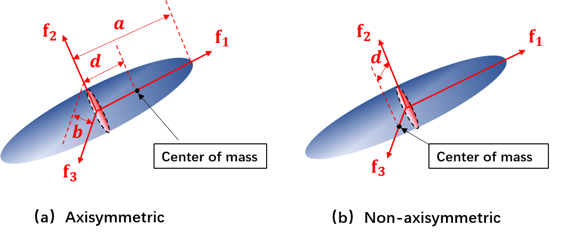
Figure 1: Two typical configurations of heterogeneous micro-structured particles of prolate spheroid with axis ${\mathbf{f}}_{1}$: (a) the center of mass is on the axis of symmetry and (b) the center of mass is away from the axis of symmetry. The major semi-axis-length of the spheroidal particle is $a$, and the minor semi-axis-length of the spheroidal particle is $b$.

As illustrated in Fig. 1, we will consider two configurations of heterogeneous spheroidal particles. Denote by $a$ and $b$ the two principle semi-axis-lengths of the spheriod, and $e=a/b$ the aspect ratio. The body frame $\{{\mathbf{f}}_{i}:i=1,2,3\}$ is fixed at the centroid of the spheroidal particle with ${\mathbf{f}}_{1}$ being the axis of symmetry. Because of the axis-symmetry, the off-diagonal block $\hat{\bm{\Upsilon}}^{\rm tr}$ vanishes whereas the diagonal components of $\hat{\bm{\Upsilon}}^{\rm tt}$ and $\hat{\bm{\Upsilon}}^{\rm rr}$ are given by ($\hat{\Upsilon}^{\rm tt}_{22}=\hat{\Upsilon}^{\rm tt}_{33}$, $\hat{\Upsilon}^{\rm rr}_{22}=\hat{\Upsilon}^{\rm rr}_{33}$ and all off-diagonal components vanish by symmetry) Kim and Karrila (1991)

$$\begin{split}&\hat{\Upsilon}^{\rm tt}_{11}=\frac{{8\pi\eta a{\left(e^{2}-1\right)^{\frac{3}{2}}}}}{e{\left[{\left(2e^{2}-1\right)\ln\left(e+\sqrt{e^{2}-1}\right)-e\sqrt{e^{2}-1}}\right]}},\\ &\hat{\Upsilon}^{\rm tt}_{22}=\frac{{16\pi\eta a{\left(e^{2}-1\right)^{\frac{3}{2}}}}}{e{\left[{\left(2e^{2}-3\right)\ln\left(e+\sqrt{e^{2}-1}\right)+e\sqrt{e^{2}-1}}\right]}},\\ &\hat{\Upsilon}^{\rm rr}_{11}=\frac{{16\pi\eta a^{3}{\left(e^{2}-1\right)^{\frac{3}{2}}}}}{3e^{3}{\left[{-\ln\left(e+\sqrt{e^{2}-1}\right)+e\sqrt{e^{2}-1}}\right]}},\\ &\hat{\Upsilon}^{\rm rr}_{22}=\frac{{16\pi\eta a^{3}{\left(e^{2}-1\right)^{\frac{3}{2}}}}(e^{2}+1)}{3e^{3}{\left[{\left(2e^{2}-1\right)\ln\left(e+\sqrt{e^{2}-1}\right)-e\sqrt{e^{2}-1}}\right]}}.\end{split}$$ (43)

IV.1.1 Axisymmetric configuration

In the first configuration illustrated in Fig. 1(a), the center of mass is on the axis of symmetry with ${\mathbf{c}}=d{\mathbf{f}}_{1}$ for some $d\in[0,a)$. Inserting (42) into (34) we find the mobility tensor is given by

$$\begin{split}\hat{{\mathbf{M}}}=\mathrm{diag}\left(\frac{1}{{\hat{\Upsilon}}^{\rm tt}_{11}},\;\;\frac{1}{{\hat{\Upsilon}}^{\rm tt}_{22}}+\frac{d^{2}}{{\hat{\Upsilon}}^{\rm rr}_{22}},\;\;\frac{1}{{\hat{\Upsilon}}^{\rm tt}_{22}}+\frac{d^{2}}{{\hat{\Upsilon}}^{\rm rr}_{22}}\right).\end{split}$$ (44)

Since the center of mass locates at the axis of symmetry, it is sufficient to describe the orientation of the particle by the usual spherical coordinates ${\bm{\Theta}}=(\theta,\varphi)\in[0,\pi]\times[0,2\pi)$ for $S^{2}$ (unit sphere in ${\mathbb{R}}^{3}$), where $\theta$ is the angle between the symmetry axis ${\mathbf{f}}_{1}$ and ${\mathbf{e}}_{1}$, and $\varphi$ is the angle between ${\mathbf{e}}_{2}$ and the projected ray of ${\mathbf{f}}_{1}$ on the ${\mathbf{e}}_{2}$-${\mathbf{e}}_{3}$-plane.

For the diffusivity in the long-time limit, our goal is to evaluate the integral (35). Being axis-symmetric, this integral over ${\rm SO}(3)$ reduces to an integral on $(\theta,\varphi)$ over $S^{2}$. Moreover, we find the rotation matrix ${\mathbf{Q}}$ as (Yuan et al., 2021)

$$\begin{split}{\mathbf{Q}}(\varphi,\theta)=&\begin{bmatrix}\cos\theta&\sin\theta\cos\varphi&\sin\theta\sin\varphi\\ \sin\theta&-\cos\theta\cos\varphi&-\cos\theta\sin\varphi\\ 0&\sin\varphi&-\cos\varphi\\ \end{bmatrix},\end{split}$$ (45)

and the stationary PDF $P^{s}(\theta,\varphi)$ in orientational space is given by (c.f., (31) and (37))

$$P^{s}(\theta,\varphi)=\frac{\sin\theta\exp\Big{[}-\frac{V(\theta,\varphi)}{k_{B}T}\Big{]}}{\int_{0}^{\pi}\!\!\!\int_{0}^{2\pi}\sin\theta\exp\Big{[}-\frac{V(\theta,\varphi)}{k_{B}T}\Big{]}\;\mathrm{d}\theta\;\mathrm{d}\varphi}.$$ (46)

Inserting (44) and (45) into (35), we find the diffusivity along the axes $\{{\mathbf{e}}_{1},{\mathbf{e}}_{2},{\mathbf{e}}_{3}\}$ of the global frame as:

$$\begin{split}D^{{\rm eff}}_{11}=&k_{B}T\big{[}\hat{M}_{11}-(\hat{M}_{11}-\hat{M}_{22})\omega\big{]},\\ D^{{\rm eff}}_{22}=&k_{B}T\big{[}\hat{M}_{22}+(\hat{M}_{11}-\hat{M}_{22})\omega^{\prime}\big{]}\\ D^{{\rm eff}}_{33}=&k_{B}T\big{[}\hat{M}_{22}+(\hat{M}_{11}-\hat{M}_{22})(\omega-\omega^{\prime})\big{]},\\ \end{split}$$ (47)

where $\hat{M}_{11},\hat{M}_{22},\hat{M}_{33}$ are given by (44), and

$$\begin{split}&\omega=\int_{0}^{\pi}\!\!\!\int_{0}^{2\pi}\!\!\!P^{s}(\theta,\varphi)\sin^{2}\theta\;\mathrm{d}\theta\;\mathrm{d}\varphi,\\ &\omega^{\prime}=\int_{0}^{\pi}\!\!\!\int_{0}^{2\pi}\!\!\!P^{s}(\theta,\varphi)\cos^{2}\varphi\sin^{2}\theta\;\mathrm{d}\theta\;\mathrm{d}\varphi,\\ \end{split}$$ (48)

Once the external potential $V(\theta,\varphi)$ is prescribed, one can simply evaluate the integrals in (48) to obtain the diffusivities in (47). In general, we expect nontrivial off-diagonal components in the diffusivity tensor. For explicit results, we consider two special scenarios.

(i) The external field, e.g., a strong applied magnetic field along ${\mathbf{e}}_{1}$-direction, tends to align the spheroid axis ${\mathbf{f}}_{1}$ with ${\mathbf{e}}_{1}$. The effect of this external field can be modeled by the external potential $V(\theta,\varphi)=E_{0}\sin^{2}\theta$. By symmetry it is easy to see all off-diagonal components of diffusivity tensor ${\mathbf{D}}^{\rm eff}$ vanish and $D^{{\rm eff}}_{22}=D^{{\rm eff}}_{33}$. Moreover, by (47) we find that

$$\begin{split}D^{{\rm eff}}_{11}=&k_{B}T\big{[}\hat{M}_{11}-(\hat{M}_{11}-\hat{M}_{22})\omega\big{]},\\ D^{{\rm eff}}_{22}=&k_{B}T\big{[}\hat{M}_{22}+\frac{\hat{M}_{11}-\hat{M}_{22}}{2}\omega\big{]},\end{split}$$ (49)

Let

$$\sigma^{2}={k_{B}T\over E_{0}}$$

be the dimensionless parameter for the strength of alignment field. If $\sigma^{2}\ll 1$, i.e., the spheroid is aligned along the field direction and weakly fluctuates, by (46) the first integral in (48) is well-approximated by

$$\omega\approx{\int_{0}^{\infty}s^{3}e^{-s^{2}/\sigma^{2}}ds\over\int_{0}^{\infty}se^{-s^{2}/\sigma^{2}}ds}=\sigma^{2}.$$

Therefore, the diffusivities in (49) are approximately given by

$$\begin{split}&D^{{\rm eff}}_{11}\approx\frac{k_{B}T}{\hat{\Upsilon}^{\rm tt}_{11}}[1+(\frac{\hat{\Upsilon}^{\rm tt}_{11}}{{\hat{\Upsilon}^{\rm tt}_{22}}}-1)\sigma^{2}-\frac{\hat{\Upsilon}^{\rm tt}_{11}}{\hat{\Upsilon}^{\rm rr}_{22}}d^{2}\sigma^{2}],\\ &D^{{\rm eff}}_{22}\approx\frac{k_{B}T}{\hat{\Upsilon}^{\rm tt}_{22}}\big{[}1+\frac{\hat{\Upsilon}^{\rm tt}_{22}}{\hat{\Upsilon}^{\rm rr}_{22}}d^{2}-\frac{\sigma^{2}}{2}(1-\frac{\hat{\Upsilon}^{\rm tt}_{22}}{{\hat{\Upsilon}^{\rm tt}_{11}}})+\frac{\hat{\Upsilon}^{\rm tt}_{22}}{2\hat{\Upsilon}^{\rm rr}_{22}}d^{2}\sigma^{2}\big{]},\end{split}$$ (50)

which may be compared with the results in Yuan et al.(Yuan et al., 2021) In particular, we notice that the corrections in diffusivities because of the heterogeneities depend on $\sigma$. As the magnitude of the external field tends to infinity, we have $\sigma\to 0$, and hence

$$\begin{split}&D^{{\rm eff}}_{11}=k_{B}T\hat{M}_{11}=\frac{k_{B}T}{\hat{\Upsilon}^{\rm tt}_{11}},\\ &D^{{\rm eff}}_{22}=\frac{k_{B}T(\hat{M}_{22}+\hat{M}_{33})}{2}=\frac{k_{B}T}{\hat{\Upsilon}^{\rm tt}_{22}}(1+{\hat{\Upsilon}^{\rm tt}_{22}d^{2}\over\hat{\Upsilon}^{\rm rr}_{22}}).\end{split}$$ (51)

From the above expressions, we see that the diffusivity along the axis-direction is independent of the heterogeneity parameter $d$ since the spheroid is always aligned with the (strong) external field direction, i.e., ${\mathbf{f}}_{1}\equiv{\mathbf{e}}_{1}$. In contrast, the translational motions on the transverse plane are coupled with the rotation around the axis, giving rise to $d$-dependent diffusivity $D^{{\rm eff}}_{22}$ in the transverse directions.

(ii) At the absence of external field, i.e., $V(\theta,\varphi)\equiv 0$, by directly evaluating the integrals in (46) and (49) we find that the diffusivity tensor is indeed isotropic, and the diffusivity (along any direction) is given by

$$\begin{split}{D}^{\rm eff}&=\frac{k_{B}T}{3}\frac{{\hat{\Upsilon}}^{\rm rr}_{22}(2{\hat{\Upsilon}}^{\rm tt}_{11}+{\hat{\Upsilon}}^{\rm tt}_{22})+2d^{2}{\hat{\Upsilon}}^{\rm tt}_{22}{\hat{\Upsilon}}^{\rm tt}_{11}}{{\hat{\Upsilon}}^{\rm tt}_{11}{\hat{\Upsilon}}^{\rm tt}_{22}{\hat{\Upsilon}}^{\rm rr}_{22}}\\ &={k_{B}T\over 6\pi a\eta}(\gamma_{0}+\gamma_{d}),\end{split}$$ (52)

where

$$\begin{split}\gamma_{0}&=\frac{e\ln(e+\sqrt{e^{2}-1})}{\sqrt{e^{2}-1}},\\ \gamma_{d}&={3e^{4}\sqrt{e^{2}-1}-3e^{2}\left(2e^{2}-1\right)\ln(e+\sqrt{e^{2}-1})\over 4\left(e^{2}-1\right)^{3/2}\left(e^{2}+1\right)}{d^{2}\over a^{2}}.\end{split}$$ (53)

Compared with the Stokes-Einstein’s formula (40), we recognize the dimensionless coefficients $\gamma_{0}$ reflects the effect of shape anisotropy whereas the dimensionless coefficients $\gamma_{d}$ signifies the importance of heterogeneity. In particular, if the particle is spherical with $e=1$, the diffusivity is given by ($r=a=b$)

$${D}^{\rm eff}=\frac{k_{\text{B}}T}{6\pi\,\eta\,r}\left(1+\frac{1}{2}\frac{d^{2}}{r^{2}}\right),$$ (54)

which can be regarded as a generalization of the classic Stokes-Einstein’s formula for heterogeneous spherical particles.

In Fig. LABEL:inhomo2, we consider five different aspect ratios ($e=1,2,5,10,20$) at the absence of an external field and plot the normalized diffusivity $D^{\rm eff}/D^{\rm eff}_{0}=1+\gamma_{d}/\gamma_{0}$ versus $d/a$, where$D^{\rm eff}_{0}=D^{\rm eff}\big{|}_{d=0}$. It can be seen that the effects of heterogeneity is more pronounced for larger aspect ratio $e$. For a spherical particle the classic Stokes-Einstein’s formula underestimates the diffusivity by $12.5\%$ if the heterogeneity gives rise to $d/r=1/2$ (c.f., (54)).

IV.1.2 Non-axisymmetric configuration

In the second configuration illustrated in Fig. 1(b), the vector pointing from the centroid of the particle to the center of mass of the particle is assumed to be ${\mathbf{c}}=d{\mathbf{f}}_{2}$ for some $d\in[0,b)$. Substituting (42) with ${\mathbf{c}}=d{\mathbf{f}}_{2}$ into (34) yields

$$\begin{split}\hat{{\mathbf{M}}}=\mathrm{diag}\left(\frac{1}{{\hat{\Upsilon}}^{\rm tt}_{11}}+\frac{d^{2}}{{\hat{\Upsilon}}^{\rm rr}_{22}},\;\;\frac{1}{{\hat{\Upsilon}}^{\rm tt}_{22}},\;\;\frac{1}{{\hat{\Upsilon}}^{\rm tt}_{22}}+\frac{d^{2}}{{\hat{\Upsilon}}^{\rm rr}_{11}}\right).\end{split}$$ (55)

For this case, the center of mass deviates from the axis of symmetry and breaks the axis-symmetry and the integral (35) over ${\rm SO}(3)$ can no longer be reduced to an integral over $S^{2}$. Nevertheless, as detailed in Appendix A we recognize the homomorphism between rigid rotations in ${\rm SO}(3)$ and unit quaternions ${\mathbf{q}}\in S^{3}$ (unit sphere in ${\mathbb{R}}^{4}$), and then employ spherical coordinates ${\bm{\Theta}}=(\psi,\theta,\varphi)\in U\equiv[0,\pi]\times[0,\pi]\times[0,2\pi]$ for $S^{3}$ to parametrize unit quaternions and rotations. More precisely, a unit quaternion ${\mathbf{q}}=x_{0}+x_{1}{\mathbf{i}}+x_{2}{\mathbf{j}}+x_{3}{\mathbf{k}}$ is represented as

$$\begin{split}&x_{0}=\cos\psi,\\ &x_{1}=\sin\psi\cos\theta,\\ &x_{2}=\sin\psi\sin\theta\cos\varphi,\\ &x_{3}=\sin\psi\sin\theta\sin\varphi,\end{split}$$ (56)

and the associated rigid rotation ${\mathbf{Q}}$ in terms of ${\bm{\Theta}}=(\psi,\theta,\varphi)$ is given by (89). Moreover, the stationary PDF $P^{s}(\psi,\theta,\varphi)$ in orientational space is now given by (c.f., (31) and (37))

$$P^{s}\!(\!\psi,\!\theta,\!\varphi\!)\ \propto{\sin^{2}\psi\sin\!\!\theta\exp\!\!\Big{[}-\frac{V(\psi,\theta,\varphi)}{k_{B}T}\Big{]}}.$$ (57)

Inserting (55) and (89) into (35), we find the diffusivity along the axes $\{{\mathbf{e}}_{1},{\mathbf{e}}_{2},{\mathbf{e}}_{3}\}$ of the global frame as:

$$\begin{split}D^{\rm eff}_{11}=&k_{B}T\Big{(}\lambda_{11}\hat{M}_{11}+\lambda_{12}\hat{M}_{22}+\lambda_{13}\hat{M}_{33}\Big{)},\\ D^{\rm eff}_{22}=&k_{B}T\Big{(}\lambda_{21}\hat{M}_{11}+\lambda_{22}\hat{M}_{22}+\lambda_{23}\hat{M}_{33}\Big{)},\\ D^{\rm eff}_{33}=&k_{B}T\Big{(}\lambda_{31}\hat{M}_{11}+\lambda_{32}\hat{M}_{22}+\lambda_{33}\hat{M}_{33}\Big{)},\end{split}$$ (58)

where $\lambda_{ij}\;(i,j=1,2,3)$, listed in (90) in Appendix B, are dimensionless parameters that depends on the PDF in (57) and $\hat{M}_{11},\hat{M}_{22},\hat{M}_{33}$ listed in (55).

Once the external potential $V(\psi,\theta,\varphi)$ is prescribed, we can evaluate the integrals in (90) for $\lambda_{ij}\;(i,j=1,2,3)$ and obtain the diffusivities along each axis direction. In general, we expect nontrivial off-diagonal components in the diffusivity tensor. Below we consider two special scenarios for explicit results.

(i) The external field is a strong field along ${\mathbf{e}}_{1}$-direction that tends to align the spheroid axis ${\mathbf{f}}_{1}$ with ${\mathbf{e}}_{1}$. The effect of this external field can be modeled by the external potential $V(\psi,\theta,\varphi)=E_{0}[1-({\mathbf{f}}_{1}\cdot{\mathbf{e}}_{1})^{2}]=E_{0}[1-Q_{11}^{2}]$ $(E_{0}\gg k_{B}T)$ where the expression of $Q_{11}$ is given in $\eqref{Q electric1}_{1}$. Then up to the order of $O(\sigma^{2})$ the parameter matrix $[\lambda_{ij}]\;(i,j=1,2,3)$ are given by ($\sigma^{2}=k_{B}T/E_{0}\ll 1$)

$$\begin{bmatrix}\lambda_{ij}\end{bmatrix}=\frac{\;1}{\;2}\begin{bmatrix}2-2\sigma^{2}&{\sigma^{2}}&{\sigma^{2}}\\ {\sigma^{2}}&1-\sigma^{2}&1-\sigma^{2}\\ {\sigma^{2}}&1-\sigma^{2}&1-\sigma^{2}\\ \end{bmatrix}+o(\sigma^{2}).\qquad$$ (59)

Therefore, to the leading order approximation the diffusivities in (58) are given by

$$\begin{split}&D^{{\rm eff}}_{11}{\approx}\frac{k_{B}T}{\hat{\Upsilon}^{\rm tt}_{11}}[1+\frac{\hat{\Upsilon}^{\rm tt}_{11}d^{2}}{\hat{\Upsilon}^{\rm rr}_{22}}+\frac{1}{2}(\frac{2\hat{\Upsilon}^{\rm tt}_{11}}{{\hat{\Upsilon}^{\rm tt}_{22}}}+\frac{\hat{\Upsilon}^{\rm tt}_{11}d^{2}}{\hat{\Upsilon}^{\rm rr}_{11}}-\frac{2\hat{\Upsilon}^{\rm tt}_{11}d^{2}}{\hat{\Upsilon}^{\rm rr}_{22}}-2)\sigma^{2}],\\ &D^{{\rm eff}}_{22}=D^{{\rm eff}}_{33}{\approx}\frac{k_{B}T}{\hat{\Upsilon}^{\rm tt}_{22}}\Big{[}1+\frac{\hat{\Upsilon}^{\rm tt}_{22}d^{2}}{2\hat{\Upsilon}^{\rm rr}_{11}}\\ &\quad\qquad\qquad+\frac{1}{2}(\frac{\hat{\Upsilon}^{\rm tt}_{22}}{{\hat{\Upsilon}^{\rm tt}_{11}}}+\frac{\hat{\Upsilon}^{\rm tt}_{22}d^{2}}{\hat{\Upsilon}^{\rm rr}_{22}}-\frac{\hat{\Upsilon}^{\rm tt}_{22}d^{2}}{{\hat{\Upsilon}^{\rm tt}_{11}}}-1)\sigma^{2}\Big{]}.\end{split}$$ (60)

As the magnitude of the external field tends to infinity, i.e., $\sigma\to 0$, by (60) we find that

$$\begin{split}&D^{{\rm eff}}_{11}=k_{B}T\hat{M}_{11}=k_{B}T(\frac{1}{\hat{\Upsilon}^{\rm tt}_{11}}+\frac{d^{2}}{\hat{\Upsilon}^{\rm rr}_{22}}),\\ &D^{{\rm eff}}_{22}=D^{{\rm eff}}_{33}=\frac{k_{B}T(\hat{M}_{22}+\hat{M}_{33})}{2}=k_{B}T(\frac{1}{\hat{\Upsilon}^{\rm tt}_{22}}+\frac{d^{2}}{2\hat{\Upsilon}^{\rm rr}_{11}}).\end{split}$$

We remark that unlike the axisymmetric configuration discussed earlier (c.f., (51)), the diffusivity along the axis-direction with center of mass deviating from axis depends on the deviation distance $d$ even if the spheroid is forced to align with the external field. This counterintuitive effect arises from the coupling between the rotational and translational motions (c.f., (4)), causing the fluctuation in rotations increases the fluctuation in translations and hence the diffusivity along ${\mathbf{e}}_{1}$-direction.

(ii) At the absence of external field, i.e., $V(\psi,\theta,\varphi)\equiv 0$, from the discussion in Appendix A the stationary PDF $P^{s}(\psi,\theta,\varphi)$ can be written as

$$P^{s}\!(\!\psi,\!\theta,\!\varphi\!)={1\over 2\pi^{2}}\sin^{2}\psi\sin\!\!\theta.$$ (61)

Upon directly evaluating the dimensionless parameters $\lambda_{i}$ listed in (90), we find that the diffusivity tensor is indeed isotropic, and the diffusivity (along any direction) is given by

$$\begin{split}{D}^{\rm eff}=&\frac{k_{B}T}{3}\frac{2{\hat{\Upsilon}}^{\rm rr}_{11}{\hat{\Upsilon}}^{\rm rr}_{22}({\hat{\Upsilon}}^{\rm tt}_{11}+{\hat{\Upsilon}}^{\rm tt}_{22})+d^{2}{\hat{\Upsilon}}^{\rm tt}_{11}{\hat{\Upsilon}}^{\rm tt}_{22}({\hat{\Upsilon}}^{\rm rr}_{11}+{\hat{\Upsilon}}^{\rm rr}_{22})}{{\hat{\Upsilon}}^{\rm tt}_{11}{\hat{\Upsilon}}^{\rm tt}_{22}{\hat{\Upsilon}}^{\rm rr}_{11}{\hat{\Upsilon}}^{\rm rr}_{22}}\\ =&{k_{B}T\over 6\pi a\eta}(\gamma_{0}+\gamma^{\prime}_{d}),\end{split}$$ (62)

where $\gamma_{0}$ is given by $\eqref{eq:alphad}_{1}$, and

$$\begin{split}\gamma^{\prime}_{d}&=\frac{3e^{3}\left(\left(e^{2}-2\right)\ln\left(\sqrt{e^{2}-1}+e\right)+\sqrt{e^{2}-1}e^{3}\right)}{8\left(e^{2}-1\right)^{3/2}\left(e^{2}+1\right)}\frac{d^{2}}{a^{2}}.\end{split}$$ (63)

We notice that $\gamma^{\prime}_{d}$ is distinct from $\eqref{eq:alphad}_{2}$, meaning that the heterogeneity along different directions has different effects on the diffusivity for shape anisotropy.

In Fig. LABEL:inhomo1, we consider five different aspect ratios ($e=1,2,5,10,20$) at the absence of an external field and plot the normalized diffusivity $D^{\rm eff}/D^{\rm eff}_{0}=1+\gamma^{\prime}_{d}/\gamma_{0}$ versus $d/a$. In contrast to Fig. LABEL:inhomo2, we see that the impacts of heterogeneity is more remarkable for smaller aspect ratio $e$. In summary, as demonstrated in Fig. LABEL:inhomo2 and Fig. LABEL:inhomo1 the heterogeneity could significantly increase the diffusivity of particles.

IV.2 Anomalous diffusion of a pair of elastically bonded spheroids

Based on results in Section IV.1, in this section we propose a model for anomalous diffusions by considering a pair of spheroids in a relaxation process. As illustrated in Fig. 4, suppose two identical homogeneous spheroids are bonded by some elastic ligaments. Suppose the axes of the two spheroids are on the same plane and form an angle $\vartheta$ and the distance between the centroids of two spheroids is given by $d$. We are interested in the long-time diffusivity of such a microstructured particle and how the diffusivity depends on the angle and distance $(\vartheta,d)$ and external fields.

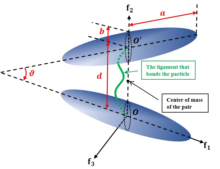
Figure 4: A simple geometric structure of the pair of spheroidal micro-structured particles with only 2 degrees of freedom. The semi-axis-length parallel to the axis of symmetry of the particle is $a$, and the semi-axis-length perpendicular to the axis of symmetry of the particle is $b$. The two spheroids are bonded by some ligaments (green line)

For simplicity, we neglect the hydrodynamic interactions between the two spheroids in the sense that the force and torque on the centroid of each spheroid is given by (1) with the drag tensor in the body frame specified by (43). By a free-body-diagram analysis, we find the nonzero components of the blocks of the drag matrix for the pair with axis angle and separation distance $(\vartheta,d)$ can be written as

$$\begin{split}\hat{R}^{\rm tt}_{11}(d,\vartheta)=&\hat{\Upsilon}^{\rm tt}_{11}+\hat{\Upsilon}^{\rm tt}_{22}+(\hat{\Upsilon}^{\rm tt}_{11}-\hat{\Upsilon}^{\rm tt}_{22})\cos\vartheta,\\ \hat{R}^{\rm tt}_{22}(d,\vartheta)=&\hat{\Upsilon}^{\rm tt}_{11}+\hat{\Upsilon}^{\rm tt}_{22}-(\hat{\Upsilon}^{\rm tt}_{11}-\hat{\Upsilon}^{\rm tt}_{22})\cos\vartheta,\\ \hat{R}^{\rm tt}_{33}(d,\vartheta)=&2\hat{\Upsilon}^{\rm tt}_{22},\\ \hat{R}^{\rm rr}_{11}(d,\vartheta)=&\frac{d^{2}\hat{\Upsilon}^{\rm tt}_{22}}{2}+(\hat{\Upsilon}^{\rm rr}_{11}-\hat{\Upsilon}^{\rm rr}_{22})\cos\vartheta+\hat{\Upsilon}^{\rm rr}_{11}+\hat{\Upsilon}^{\rm rr}_{22}\\ \hat{R}^{\rm rr}_{22}(d,\vartheta)=&(\hat{\Upsilon}^{\rm rr}_{22}-\hat{\Upsilon}^{\rm rr}_{11})\cos\vartheta+\hat{\Upsilon}^{\rm rr}_{11}+\hat{\Upsilon}^{\rm rr}_{22},\\ \hat{R}^{\rm rr}_{33}(d,\vartheta)=&\frac{1}{4}\left(d^{2}(\hat{\Upsilon}^{\rm tt}_{11}-\hat{\Upsilon}^{\rm tt}_{22})\cos\vartheta+d^{2}(\hat{\Upsilon}^{\rm tt}_{11}+\hat{\Upsilon}^{\rm tt}_{22})+8\hat{\Upsilon}^{\rm rr}_{22}\right)\\ \hat{R}^{\rm tr}_{32}(d,\vartheta)=&\frac{1}{2}d(\hat{\Upsilon}^{\rm tt}_{11}-\hat{\Upsilon}^{\rm tt}_{22})\sin\vartheta,\\ \end{split}$$ (64)

where $\hat{{\Upsilon}}^{\rm tt}_{11},\hat{{\Upsilon}}^{\rm tt}_{22}$ and $\hat{{\Upsilon}}^{\rm rr}_{11},\hat{{\Upsilon}}^{\rm rr}_{22}$, given by (43), are the components of the diagonal blocks of the drag matrix for a single spheroid.

We first consider the diffusion of the pair with fixed $(d,\vartheta)$. At the absence of external fields, the stationary PDF $P^{s}(\psi,\theta,\varphi)$ is given by (91). Upon repeating the procedure from (55) to (62), we find that the diffusivity tensor is indeed isotropic, and the diffusivity (along any direction) is given by

$$\begin{split}&D^{\rm eff}(\vartheta,d)=\!\!\!\frac{k_{B}T}{3}\!\Big{[}\frac{1}{2\hat{\Upsilon}^{\rm tt}_{22}}+\frac{1}{2\hat{\Upsilon}^{\rm tt}_{11}\cos^{2}\frac{\vartheta}{2}+2\hat{\Upsilon}^{\rm tt}_{22}\sin^{2}\frac{\vartheta}{2}}+\\ &\quad+\frac{4\hat{\Upsilon}^{\rm rr}_{22}+d^{2}(\hat{\Upsilon}^{\rm tt}_{11}\cos^{2}\frac{\vartheta}{2}+\hat{\Upsilon}^{\rm tt}_{22}\sin^{2}\frac{\vartheta}{2})}{8\hat{\Upsilon}^{\rm rr}_{22}(\hat{\Upsilon}^{\rm tt}_{11}\sin^{2}\frac{\vartheta}{2}+\hat{\Upsilon}^{\rm tt}_{22}\cos^{2}\frac{\vartheta}{2})+2d^{2}\hat{\Upsilon}^{\rm tt}_{11}\hat{\Upsilon}^{\rm tt}_{22}}\Big{]}.\end{split}$$ (65)

As $d\to+\infty$, i.e., the two spheroids are far apart, we have

$$\begin{split}D^{\rm eff}\to&\frac{k_{B}T}{3}\!\Big{[}\frac{1}{2\hat{\Upsilon}^{\rm tt}_{22}}+\frac{(\hat{\Upsilon}^{\rm tt}_{11}-\hat{\Upsilon}^{\rm tt}_{22})\cos\vartheta+\hat{\Upsilon}^{\rm tt}_{11}+\hat{\Upsilon}^{\rm tt}_{22}}{4\hat{\Upsilon}^{\rm tt}_{11}\hat{\Upsilon}^{\rm tt}_{22}}\\ &+\frac{1}{(\hat{\Upsilon}^{\rm tt}_{11}-\hat{\Upsilon}^{\rm tt}_{22})\cos\vartheta+\hat{\Upsilon}^{\rm tt}_{11}+\hat{\Upsilon}^{\rm tt}_{22}}\Big{]}.\end{split}$$ (66)

In particular, if $\vartheta=0$ or $\vartheta=\pi$, i.e., the two spheroids are aligned, we have

$$\begin{split}D^{\rm eff}=\frac{k_{B}T}{6}\Big{[}\frac{1}{\hat{\Upsilon}^{\rm tt}_{11}}+\frac{2}{\hat{\Upsilon}^{\rm tt}_{22}}\Big{]},\end{split}$$ (67)

which can also be derived from (38) since ${\mathbf{R}}^{\rm tr}={\bf 0}$.

If, in particular, the spheroid is a ball such that $\hat{\Upsilon}^{\rm tt}_{22}=\hat{\Upsilon}^{\rm tt}_{11}$,

$$D^{\rm eff}=\frac{k_{B}T}{2\hat{\Upsilon}^{\rm tt}_{11}},$$

which is precisely half of the diffusivity of a single spherical particle.

To see the influence of structural parameters $(\vartheta,d)$ of the pair on the long-time diffusivity, we consider two cases: a pair of prolates with major and minor semi-axis-length $1\mu m$ and $0.1\mu m$, respectively, and a pair of oblates with the same volume and minor axis-length. In Fig. 5 we plot the normalized diffusivity $D^{\rm eff}/D^{\rm eff}_{0}$ versus $\vartheta$ for $d=2\mu m$, where $D^{0}=\frac{k_{B}T}{3}{{\rm Tr}}\;[\hat{{\bm{\Upsilon}}}^{{\rm tt}^{-}1}]$ denotes the diffusivity of a single spheroid. Meanwhile, the normalized diffusivity $D^{\rm eff}/D^{\rm eff}_{0}$ is plotted against $d$ in Fig. 6 for $\vartheta=\pi/2$.

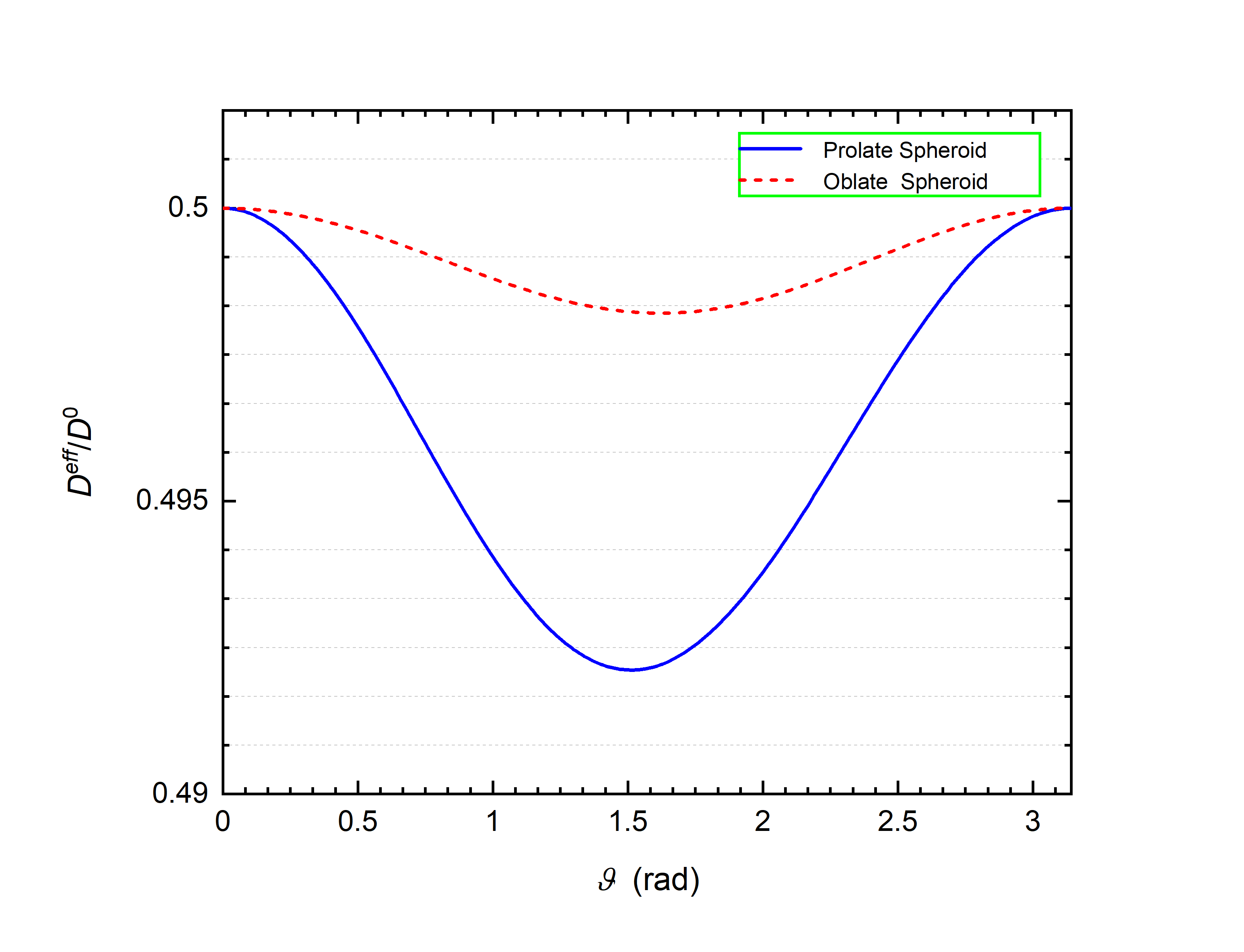
Figure 5: The nondimensionalized long-time diffusivity $\frac{{D}^{\rm eff}}{D^{0}}$ of the pair of spheroids (as illustrated in Fig.4) versus the angle $\vartheta$ between two axes of spheroids. The major and minor semi-axis-length of spheroid are $1\mu m$ and $0.1\mu m$ for prolate spheroids (blue), respectively. The oblate spheroids (red) have the same volume and minor-axis length. The distance $d$ between the centroids of the two particles is fixed at $2\mu m$.

Figure 6: The nondimensionalized long-time diffusivity $\frac{{D}^{\rm eff}}{D^{0}}$ of the pair of spheroids (as illustrated in Fig.4) versus the distance $d$ between two spheroids. The major and minor semi-axis-length of spheroid are $1\mu m$ and $0.1\mu m$ for prolate spheroids (blue), respectively. The oblate spheroids (red) have the same volume and minor-axis length. The angle $\vartheta$ between the two axes of symmetry is fixed at $\frac{\pi}{2}$.

From Fig. 5 we see that the diffusivity ${D}^{\rm eff}$ of the pair is unsurprisingly lower than that of a single particle since the size of the pair is larger (c.f., the Stokes-Einstein relation (40)). On the other hand, there exist some optimal angles $\vartheta\in[0,\pi]$ for which the diffusivity ${D}^{\rm eff}$ of the pairs is either minimized or maximized. From Fig. 6 we see that the long-time diffusivity monotonically increases with $d$ until the curves flatten out, as is expected by (65) and (66).

Based on the explicit formula (65), we next consider the model of a pair of spheroids whose relative angle and distance depends on time. Suppose the relative angle and distance pair are initially given by $(\vartheta_{0},d_{0})$ and the elastic ligament is not fully relaxed. Because of the elastic energy in the ligament, we anticipate the relaxation of angle and distance can be characterized by two relaxation time scales (${\tau^{*}_{1}},\tau^{\ast}_{2}$) in the sense that the time-dependent angle and distance are given by

$$\begin{split}\vartheta(t)&=\vartheta_{f}+(\vartheta_{0}-\vartheta_{f})e^{-\frac{t}{\tau^{*}_{1}}},\\ d(t)&=\mathrm{d}_{f}+(\mathrm{d}_{0}-\mathrm{d}_{f})e^{-\frac{t}{\tau^{*}_{2}}},\\ \end{split}$$ (68)

where $(\vartheta_{f},d_{f})$ denote the angle and distance between the pair in the final equilibrium state.

In typical experimental measurements, the diffusivity or anomalous diffusion is characterized by the Mean Square Displacement ($MSD$) defined by (Metzler et al., 2014)

$$MSD(t):=\frac{1}{t_{m}}\int_{0}^{t_{m}}|{\mathbf{x}}(t^{\prime}+t)-{\mathbf{x}}(t^{\prime})|^{2}\;\mathrm{d}t^{\prime},$$ (69)

where ${\mathbf{x}}(t)$ is the position of the center of mass of the pair, and $t_{m}$ is the total measure time. For normal diffusions with a single time scale, e.g., diffusion of a homogeneous rigid spherical particle, the scaling of $MSD$ in (72) with respect to time satisfies

$${MSD(t)\over 2t}\to{D}\qquad{{\rm\;as\;}}\;t\to+\infty,$$ (70)

where $D$ is the macroscopic diffusivity. Now we consider the scaling of $MSD$ with respect to time for the pair of spheroids that relax from an initial non-equilibrium state. From the prior discussions, this process involves at least four time scales: cross-over time scale $t_{cross}$ (c.f., (28)), the two relaxation time scales $\tau^{*}_{1},\tau^{*}_{2}$ for evolution of the relative angle and distance $(\vartheta,d)$ between the pair, and the translation diffusion time-scale of the pair. Therefore, the $MSD$ of the pair should exhibit much more complicated scaling behaviors with respect to $t$.

Nevertheless, if there is separation of time scales in the sense that

$$t\gg\tau^{*}_{1},\tau^{*}_{2}\gg t_{cross},$$

by (70) we expect that $MSD$ should approximately behave as

$$MSD(t)\approx 2t{D}^{\rm eff}(\vartheta(t),d(t)),$$ (71)

where the diffusivity ${D}^{\rm eff}(\vartheta(t),d(t))$ is given by (65) and $(\vartheta(t),d(t))$ is specified by (68).

For comparison, let

$$MSD_{0}(t)=2t{D}^{\rm eff}(\vartheta_{0},d_{0}),$$ (72)

denote the Mean Square Displacement for the normal diffusion of the pair with $\vartheta(t)\equiv\vartheta_{0}$ and $d(t)\equiv d_{0}$. Then, in Fig. 7, we plot the difference $\Delta MSD=MSD-MSD_{0}$ between the MSDs of the center of mass of the pair against $t$ for two cases. Specifically, the distance $d_{f}$ between the pair in the final equilibrium state is set to be $4a$ for case 1, whereas the distance $d_{f}$ between the pair in the final equilibrium state is set to be $2a$ for case 2. The initial distance $d_{0}$ between the pair in the initial non-equilibrium state is set to be $3a$ for both cases.

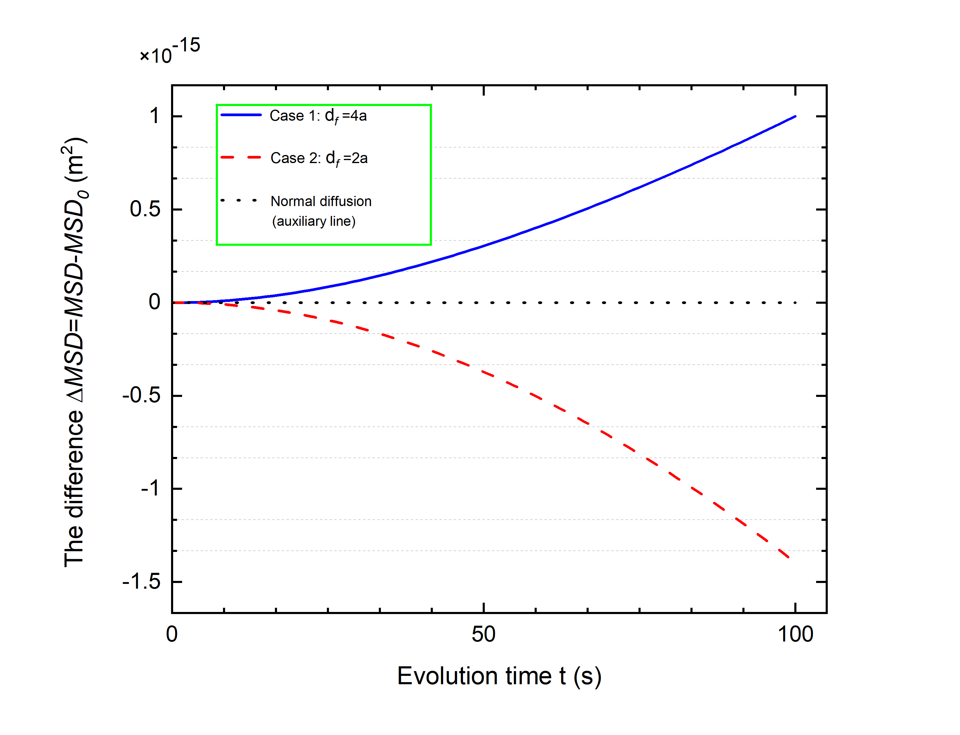
Figure 7: The difference $\Delta MSD=MSD-MSD_{0}$ between the MSDs of the center of mass of the pair against time $t$ for two cases. The blue line refers to case 1 for which the final equilibrium distance $d_{f}=4a$, whereas the red line refers to case 2 with the final equilibrium distance $d_{f}=2a$. The distance between the pair in the initial non-equilibrium is $d_{0}=3a$. The major and minor semi-axis-lengths of the particle are $1\mu m$ and $0.1\mu m$, respectively. The angle $\vartheta$ between the axes of symmetry of the pair of the particles is fixed at $\frac{\pi}{2}$. The relaxing time-scale is assumed to be $\tau^{*}_{2}=100s$. The ambient fluid is the mineral oil with viscosity $\eta=12.7\times 10^{-3}\;N\cdot s/m^{2}$.

From Fig. 7 we observe two different types of scalings fo MSD versus $t$, which may be interpreted as “superdiffusion” and “subdiffusion”, respectively. From this viewpoint, we expect physical models like ours could shed light on many anomalous diffusions observed in biological systems and complex media.

V Conclusion remarks

In summary, we have conducted a systematic analysis on the long-time diffusion of microstructured particles of arbitrary shape and heterogeneity in a Newtonian fluid. The microscopic Brownian dynamics in position-orientation space is coarse-grained into a Fokker-Planck equation governing the evolution of the PDF on ${\mathbb{R}}^{3}\times{\rm SO}(3)$. By analyzing the Fokker-Planck equation, we identify a formula for the long-time diffusivity of the microstructured particle in an alignment field (c.f., (33) or (35)). Applied to heterogeneous spheroids, we discover generalizations of the classical Stokes-Einstein relation which assert that the diffusivity of a rigid heterogeneous particle depends on the deviation of the center of mass from the geometric centroid (c.f., (52), (54) and (62)). We have also addressed the effects of an external alignment field and achieved leading-order corrections on the diffusivities for large alignment fields (c.f., (50) and (60)). Based on these results, we consider diffusion of a pair of spheroids bonded by elastic ligaments. If the pair are initially in a non-equilibrium state, the Brownian motion superimposed with the relaxation process could be characterized as apparent “superdiffusion” or “subdiffusion”, entailing a mechanistic perspective on anomalous diffusions. We believe that our method and results lay a solid foundation for understanding diffusions in complex media and may inspire new applications of controlled diffusions in biophysics and materials science.

Appendix A Evaluation of integrals over ${\rm SO}(3)$

To find the effective long-time diffusivities of microstructured particles, we have to address the technical problem (35) of evaluating integrals over ${\rm SO}(3)$. A fundamental theorem in the theory of Lie group asserts that there exists a unique measure on every compact Lie group, namely, the Haar measure $d\mu_{\mathbf{Q}}$, such that the integral (Bröcker and tom Dieck, 1985)

$$I[f]=\int_{SO(3)}f({\mathbf{Q}})\mathrm{d}\mu_{\mathbf{Q}}$$ (73)

is normalized (i.e., $I[1]=1$) and (left-)invariant:

$$I[f({\mathbf{Q}})]=I[f({\mathbf{Q}}^{\prime}{\mathbf{Q}})]\quad\forall\;{\mathbf{Q}}^{\prime}\in{\rm SO}(3).$$

The integral (35) should be interpreted as in (73) for the Haar measure.

In practice, we need a parametrization of ${\rm SO}(3)$ to carry out the integral (73) explicitly. Here we employ the quaternion representation of ${\rm SO}(3)$. A quaternion ${\mathbf{q}}$ can be written as

$${\mathbf{q}}=x_{0}+x_{1}{\mathbf{i}}+x_{2}{\mathbf{j}}+x_{3}{\mathbf{k}},$$ (74)

where ${\mathbf{i}},{\mathbf{j}},{\mathbf{k}}$ are three (linearly independent) symbols. Equipped with the regular scalar product and vector addition, the collection of quaternions form a four-dimensional vector space. The norm of a quaternion is defined as

$$|{\mathbf{q}}|^{2}=x_{0}^{2}+x_{1}^{2}+x_{2}^{2}+x_{3}^{2}.$$ (75)

Non-commutative multiplications between quaternions are defined by requiring the following relations:

$$\begin{split}&{\mathbf{i}}^{2}={\mathbf{j}}^{2}={\mathbf{k}}^{2}={\mathbf{i}}{\mathbf{j}}{\mathbf{k}}=-1.\end{split}$$ (76)

From (76) it is straightforward to verify

$$\begin{split}&{\mathbf{i}}{\mathbf{j}}=-{\mathbf{j}}{\mathbf{i}}={\mathbf{k}};\;\;{\mathbf{j}}{\mathbf{k}}=-{\mathbf{k}}{\mathbf{j}}={\mathbf{i}};\;\;{\mathbf{k}}{\mathbf{i}}=-{\mathbf{i}}{\mathbf{k}}={\mathbf{j}}.\end{split}$$ (77)

Therefore, the multiplication of two quaternions ${\mathbf{q}}_{1}=(u_{1},{\mathbf{v}}_{1})$ and ${\mathbf{q}}_{2}=(u_{1},{\mathbf{v}}_{2})$ ($u_{1},u_{2}\in{\mathbb{R}}$ and ${\mathbf{v}}_{1},{\mathbf{v}}_{2}\in{\mathbb{R}}^{3}$) can be written as

$${\mathbf{q}}_{1}{\mathbf{q}}_{2}=(u_{1}u_{2}-{\mathbf{v}}_{1}\cdot{\mathbf{v}}_{2})+u_{1}{\mathbf{v}}_{2}+u_{2}{\mathbf{v}}_{1}+{\mathbf{v}}_{1}\times{\mathbf{v}}_{2},$$ (78)

where ‘$\cdot$’ and ‘$\times$’ denote the familiar dot product and cross product, respectively. Define $\overline{{\mathbf{q}}}=(x_{0},-{\mathbf{x}})$ as the conjugate of ${\mathbf{q}}=(x_{0},{\mathbf{x}})$. From (78) it is straightforward to verify that

$$|{\mathbf{q}}|^{2}={\mathbf{q}}\overline{{\mathbf{q}}}=x_{0}x_{0}+{\mathbf{x}}\cdot{\mathbf{x}}\quad{{\rm\;\;and\;\;}}\quad\overline{{\mathbf{q}}_{1}{\mathbf{q}}_{2}}=\overline{{\mathbf{q}}}_{2}\overline{{\mathbf{q}}}_{1}.$$ (79)

Therefore, the inverse ${\mathbf{q}}^{-1}$ of a unit quaternion ${\mathbf{q}}\in S^{3}$, i.e., the quaternion such that ${\mathbf{q}}{\mathbf{q}}^{-1}={\mathbf{q}}^{-1}{\mathbf{q}}=1$, is precisely the conjugate $\overline{{\mathbf{q}}}$. In addition, for two unit quaternions ${\mathbf{q}}_{1},{\mathbf{q}}_{2}$, by (78) we have

$$|{\mathbf{q}}_{1}{\mathbf{q}}_{2}|^{2}={\mathbf{q}}_{1}{\mathbf{q}}_{2}\overline{{\mathbf{q}}_{1}{\mathbf{q}}_{2}}=|{\mathbf{q}}_{2}|^{2}|{\mathbf{q}}_{1}|^{2}=1.$$

In conclusion, the collection of unit quaternions equipped with multiplication (78) forms a continuous compact group.

Next, we construct a homomorphism $h:S^{3}\to{\rm SO}(3)$ from the group of unit quaternions to the group of rigid rotations. Let ${\mathbf{Q}}=h({\mathbf{q}})$ and $\tilde{{\mathbf{p}}}=(0,{\mathbf{p}})$ be the quaternion associated with a vector ${\mathbf{p}}\in{\mathbb{R}}^{3}$. For a given unit quaternion ${\mathbf{q}}\in S^{3}$, the map ${\mathbf{q}}\mapsto{\mathbf{Q}}=h({\mathbf{q}})$ is defined by requiring that for any ${\mathbf{p}}\in{\mathbb{R}}^{3}$,

$$\begin{split}{\mathbf{p}}^{\prime}=&{\mathbf{q}}\tilde{{\mathbf{p}}}{\mathbf{q}}^{-1}\quad\mathrm{quaternion\;multiplication}\\ =&{\mathbf{Q}}{\mathbf{p}}\;\quad\quad\mathrm{matrix\;product}.\\ \end{split}$$ (80)

For a unit quaternion ${\mathbf{q}}$ given by (74), the above equation implies

$$\begin{split}{\mathbf{p}}^{\prime}\!&=\!({\mathbf{p}}\cdot{\mathbf{x}}){\mathbf{x}}\!+\!x_{0}(x_{0}{\mathbf{p}}-{\mathbf{p}}\!\times\!{\mathbf{x}})\!+\!{\mathbf{x}}\!\times\!(x_{0}{\mathbf{p}}-{\mathbf{p}}\!\times\!{\mathbf{x}})\\ &={\mathbf{Q}}{\mathbf{p}}\qquad\forall\;{\mathbf{p}}\in{\mathbb{R}}^{3},\end{split}$$ (81)

and hence,

$${\mathbf{Q}}=(x_{0}^{2}-|{\mathbf{x}}|^{2}){\mathbf{I}}+2{\mathbf{x}}\otimes{\mathbf{x}}+2x_{0}{\mathbf{W}}_{\mathbf{x}},$$ (82)

where ${\mathbf{W}}_{\mathbf{x}}$ is the skew-symmetric matrix such that ${\mathbf{W}}_{\mathbf{x}}{\mathbf{p}}={\mathbf{x}}\times{\mathbf{p}}$ for any ${\mathbf{p}}\in{\mathbb{R}}^{3}$. Conversely, for any ${\mathbf{Q}}\in{\rm SO}(3)$ we solve (82) for the unit quaternion ${\mathbf{q}}$ and find that

$$\begin{split}&x_{0}=\frac{\sqrt{1+{{\rm Tr}}{\mathbf{Q}}}}{2},\\ &x_{1}={\rm sgn}(Q_{32}-Q_{23})|\frac{1}{2}\sqrt{1+{{\rm Tr}}{\mathbf{Q}}-2Q_{22}-2Q_{33}}|,\\ &x_{2}={\rm sgn}(Q_{13}-Q_{31})|\frac{1}{2}\sqrt{1+{{\rm Tr}}{\mathbf{Q}}-2Q_{11}-2Q_{33}}|,\\ &x_{3}={\rm sgn}(Q_{21}-Q_{12})|\frac{1}{2}\sqrt{1+{{\rm Tr}}{\mathbf{Q}}-2Q_{11}-2Q_{22}}|,\\ \end{split}$$

where ‘${\rm sgn}$’ denotes the sign function.

From (80), we find that for any two unit quarternions ${\mathbf{q}}_{i}\in S^{3}$ and ${\mathbf{Q}}_{i}=h({\mathbf{q}}_{i})$ ($i=1,2$),

$$\begin{split}({\mathbf{q}}_{2}{\mathbf{q}}_{1})\tilde{{\mathbf{p}}}({\mathbf{q}}_{2}{\mathbf{q}}_{1})^{-1}={\mathbf{q}}_{2}({\mathbf{q}}_{1}\tilde{{\mathbf{p}}}{\mathbf{q}}_{1}^{{-1}}){\mathbf{q}}_{2}^{{-1}}\\ ={\mathbf{q}}_{2}(0,{\mathbf{Q}}_{1}{\mathbf{p}}){\mathbf{q}}_{2}^{{-1}}=(0,{\mathbf{Q}}_{2}{\mathbf{Q}}_{1}{\mathbf{p}}),\end{split}$$ (83)

which means

$$h({\mathbf{q}}_{2}{\mathbf{q}}_{1})=h({\mathbf{q}}_{2})h({\mathbf{q}}_{1}).$$ (84)

That is, the map ${\mathbf{q}}\mapsto{\mathbf{Q}}=h({\mathbf{q}})$ defined by (80) is a homomorphism. Therefore, the integral (73) over ${\rm SO}(3)$ can be rewritten as integrals over $S^{3}$:

$$I[f]=\int_{SO(3)}f({\mathbf{Q}})\mathrm{d}\mu_{\mathbf{Q}}=\int_{S^{3}}f({\mathbf{Q}}({\mathbf{q}}))\mathrm{d}\mu_{\mathbf{q}},$$ (85)

where $\mu_{\mathbf{q}}$ represents the Haar measure on the group of unit quaternions. On $S^{3}$, for any fixed unit quaternion ${{\bm{\alpha}}}\in S^{3}$ and ${\mathbf{q}}^{\prime}={{\bm{\alpha}}}{\mathbf{q}}$ we have

$$d{\mathbf{q}}^{\prime}\cdot d{\mathbf{q}}^{\prime}=({{\bm{\alpha}}}d{\mathbf{q}})\overline{{{\bm{\alpha}}}d{\mathbf{q}}}=d{\mathbf{q}}\cdot d{\mathbf{q}}(\alpha\overline{\alpha})=d{\mathbf{q}}\cdot d{\mathbf{q}}.$$

That is, the usual (normalized) Lebesgue measure is invariant, and hence the Haar measure.

Finally, we parametrize $S^{3}$ by the standard spherical coordinates ${\bm{\Theta}}=(\psi,\theta,\varphi)\in U\equiv[0,\pi]\times[0,\pi]\times[0,2\pi]$ so that a unit quaternion ${\mathbf{q}}\in S^{3}$ can be represented as (74) with

$$\begin{split}&x_{0}=\cos\psi,\\ &x_{1}=\sin\psi\cos\theta,\\ &x_{2}=\sin\psi\sin\theta\cos\varphi,\\ &x_{3}=\sin\psi\sin\theta\sin\varphi.\end{split}$$ (86)

Then the (normalized) Lebesgue measure on $S^{3}$ can be written as

$$d\mu_{\mathbf{q}}\!\propto|\det({\mathbf{g}}^{T}{\mathbf{g}})|^{1/2}\mathrm{d}\psi\mathrm{d}\theta\mathrm{d}\varphi=\sin^{2}\psi\sin\theta\mathrm{d}\psi\mathrm{d}\theta\mathrm{d}\varphi,$$

where ${\mathbf{g}}$ is the $4\times 3$ Jacobian matrix:

$${\mathbf{g}}={\partial(x_{0},x_{1},x_{2},x_{3})\over\partial(\psi,\theta,\varphi)}.$$

By direct integration we find the volume of the hypersurface $S^{3}$ is given by

$$V_{0}=\int_{U}\sin^{2}\psi\sin\theta\mathrm{d}\psi\mathrm{d}\theta\mathrm{d}\varphi=2\pi^{2}.$$ (87)

Consequently, by (85) we conclude that the integral (73) can be calculated by

$$I[f]\!\!={1\over 2\pi^{2}}\int_{U}f({\mathbf{Q}}(\psi,\theta,\varphi))\sin^{2}\psi\sin\theta\mathrm{d}\psi\mathrm{d}\theta\mathrm{d}\varphi$$ (88)

where ${\mathbf{Q}}(\psi,\theta,\varphi)$, by (82) and (86), is given by

$$\begin{split}Q_{11}=&\frac{2\cos 2\psi-\cos 2(\psi-\theta)+2\cos 2\theta-\cos 2(\psi+\theta)+2}{4};\\ Q_{21}=&2\sin\psi\sin\theta(\cos\theta\cos\varphi\sin\psi+\cos\psi\sin\varphi);\\ Q_{31}=&2\sin\psi\sin\theta(\cos\theta\sin\psi\sin\varphi-\cos\psi\cos\varphi);\\ Q_{12}=&2\sin\psi\sin\theta(\cos\theta\cos\varphi\sin\psi-\cos\psi\sin\varphi);\\ Q_{22}=&\cos^{2}\psi+\sin^{2}\psi\left(\cos 2\varphi\sin^{2}\theta-\cos^{2}\theta\right);\\ Q_{32}=&2\sin\psi\left(\cos\varphi\sin\psi\sin\varphi\sin^{2}\theta+\cos\psi\cos\theta\right);\\ Q_{13}=&2\sin\psi\sin\theta(\cos\psi\cos\varphi+\cos\theta\sin\psi\sin\varphi);\\ Q_{23}=&2\sin\psi\left(\cos\varphi\sin\psi\sin^{2}\theta\sin\varphi-\cos\psi\cos\theta\right);\\ Q_{33}=&\cos^{2}\psi-\sin^{2}\psi\left(\cos^{2}\theta+\cos 2\varphi\sin^{2}\theta\right).\end{split}$$ (89)

Appendix B The expressions of $\lambda_{ij}$ in (58)

Inserting (89) into (35), we can write the diagonal components of the diffusivity tensor (35) as (58). Recall that the mobility tensor $\hat{{\mathbf{M}}}$ in (35) is given by (55) and the rigid rotation matrix ${\mathbf{Q}}(\Theta)$ in (35) is listed in (89). Straightforward algebraic calculations yield the expressions of $\lambda_{ij}\;(i,j=1,2,3)$ in terms of $(\psi,\theta,\varphi)$ as follows:

$$\begin{split}\lambda_{ij}=\!\!\!\int_{U}Q_{ij}^{2}(\psi,\theta,\varphi)P^{s}(\psi,\theta,\varphi)\mathrm{d}\psi\mathrm{d}\theta\mathrm{d}\varphi.\end{split}$$ (90)

For heterogeneous spheroids as illustrated in Fig. 1 (b), if the external field is large in the sense that $\sigma^{2}=k_{B}T/E_{0}\ll 1$, then the PDF in (57) can be approximated by

$$\begin{split}P^{s}\!(\!\psi,\!\theta,\!\varphi\!)&\propto{\sin^{2}\psi\sin\!\!\theta\exp\!\!\Big{[}-\frac{E_{0}(1-Q_{11}^{2})}{k_{B}T}\Big{]}}\int_{0}^{\pi}\;d\theta\\ &\approx{\sin^{2}\psi\sin\!\!\theta\exp\!\!\Big{[}-\frac{4\theta^{2}(\sin\psi)^{2}}{\sigma^{2}}\Big{]}}\int_{0}^{\infty}\;d\theta.\end{split}$$ (91)

By this approximation and direct integration, we obtain the approximate values of $\lambda_{ij}\;(i,j=1,2,3)$ as given by (59) in the main text.

Acknowlegement

The authors thank Prof. Jian Song for insightful discussions.

References

• Einstein (1905) A. Einstein, “On the motion of small particles suspended in liquids at rest required by the molecular-kinetic theory of heat,” Ann. Phys. (Berlin) 17, 549–560 (1905).
• Perrin (1908) J. Perrin, “Les preuves de la réalite moléculaire,” Comptes Rendus 147, 530–532 (1908).
• Ende and Peppas (1995) M. Ende and N. Peppas, “Analysis of fickian and non-fickian drug release from polymers,” Pharm Acta Helv. 12, 2030–2035 (1995).
• Jain (1987) R. Jain, “Transport of molecules in the tumor interstitium: a review.” Cancer Res. 47, 3039–51 (1987).
• Bangham, Standish, and Watkins (1965) A. Bangham, M. Standish,  and J. Watkins, “Diffusion of univalent ions across the lamellae of swollen phospholipids,” Journal of Molecular Biology 13, 238–IN27 (1965).
• Perrin (1934) F. Perrin, “Mouvement brownien d’un ellipsoide-i. dispersion diélectrique pour des molécules ellipsoidales,” J. Phys. Radium V 5 (1934).
• Perrin (1936) F. Perrin, “Mouvement brownien d’un ellipsoide (ii). rotation libre et dépolarisation des fluorescences. translation et diffusion de molécules ellipsoidales,” J. Phys. Radium VII 7 (1936).
• Han et al. (2006) Y. Han, A. Alsayed, M. Nobili, J. Zhang, T. Lubensky,  and A. Yodh, “Brownian motion of an ellipsoid,” Science 314, 626–630 (2006).
• Han et al. (2009) Y. Han, A. Alsayed, M. Nobili,  and A. Yodh, “Quasi-two-dimensional diffusion of single ellipsoids: Aspect ratio and confinement effects,” Phys. Rev. E 80, 011403 (2009).
• Duggal and Pasquali (2006) R. Duggal and M. Pasquali, “Dynamics of individual single-walled carbon nanotubes in water by real-time visualization,” Phys. Rev. Lett. 96, 246104 (2006).
• Cheong and Grier (2010) F. Cheong and D. Grier, “Rotational and translational diffusion of copper oxide nanorods measured with holographic video microscopy,” Opt. Express 18, 6555–6562 (2010).
• Bhaduri, Neild, and Ng (2008) B. Bhaduri, A. Neild,  and T. W. Ng, “Directional brownian diffusion dynamics with variable magnitudes,” Applied Physics Letters 92, 084105 (2008).
• Kraft et al. (2013) D. J. Kraft, R. Wittkowski, B. ten Hagen, K. V. Edmond, D. J. Pine,  and H. Löwen, “Brownian motion and the hydrodynamic friction tensor for colloidal particles of complex shape,” Phys. Rev. E 88, 050301 (2013).
• Maragó (2010) O. t. Maragó, “Brownian motion of graphene,” ACS nano 4, 7515–7523 (2010).
• Chakrabarty et al. (2014) A. Chakrabarty, A. Konya, F. Wang, J. Selinger, K. Sun,  and Q. Wei, “Brownian motion of arbitrarily shaped particles in two dimensions,” Langmuir 30, 13844–13853 (2014).
• Köster, Steinhauser, and Pfohl (2005) S. Köster, D. Steinhauser,  and T. Pfohl, “Brownian motion of actin filaments in confining microchannels,” J. Phys. Condens. Matter 17, S4091 (2005).
• Koens and Lauga (2014) L. Koens and E. Lauga, “The passive diffusion of Leptospira interrogans,” Physical Biology 11, 066008 (2014).
• Brenner (1964) H. Brenner, “The stokes resistance of an arbitrary particle—ii: An extension,” Chemical Engineering Science 19, 599–629 (1964).
• Brenner (1967) H. Brenner, “Coupling between the translational and rotational brownian motions of rigid particles of arbitrary shape: Ii. general theory,” J. Colloid Interface Sci. 23, 407–436 (1967).
• Bernal and De La Torre (1980) J. M. G. Bernal and J. G. De La Torre, “Transport properties and hydrodynamic centers of rigid macromolecules with arbitrary shapes,” Biopolymers 19, 751–766 (1980).
• Harvey and Garcia de la Torre (1980) S. Harvey and J. Garcia de la Torre, “Coordinate systems for modeling the hydrodynamic resistance and diffusion coefficients of irregularly shaped rigid macromolecules,” Macromolecules 13, 960–964 (1980).
• Yuan et al. (2021) T. Yuan, W. Yuan, L. Liu,  and J. W. Shan, “Electric-field-controlled diffusion of anisotropic particles: theory and experiment,” Journal of Fluid Mechanics 924, A42 (2021).
• Castellano et al. (2015) R. Castellano, C. Akin, G. Giraldo, S. Kim, F. Fornasiero,  and J. Shan, “Electrokinetics of scalable, electric-field-assisted fabrication of vertically aligned carbon-nanotube/polymer composites,” J. Appl. Phys. 117, 13 (2015).
• Cetindag et al. (2017) S. Cetindag, B. Tiwari, D. Zhang, Y. Yap, S. Kim,  and J. Shan, “Surface-charge effects on the electro-orientation of insulating boron-nitride nanotubes in aqueous suspension,” J. Colloid Interface Sci. 505, 1185–1192 (2017).
• Yuan, Liu, and Shan (2017) W. Yuan, L. Liu,  and J. Shan, “Tunable acoustic attenuation in dilute suspensions of subwavelength, non-spherical magnetic particles,” J. Appl. Phys. 121, 045110 (2017).
• Squires and Bazant (2006) T. Squires and M. Bazant, “Breaking symmetries in induced-charge electro-osmosis and electrophoresis,” J. Fluid Mech. 560, 65–101 (2006).
• Yuan et al. (2019) W. Yuan, G. Tutuncuoglu, A. Mohabir, L. Liu, L. Feldman, M. Filler,  and J. Shan, “Contactless electrical and structuralcharacterization of semiconductor nanowires with axially modulated doping profiles,” Small 15, 1805140 (2019).
• Doi and Makino (2016) M. Doi and M. Makino, “Separation of chiral particles in a rotating electric field,” Physics of Fluids 28, 093302 (2016).
• Grima and Yaliraki (2007) R. Grima and S. Yaliraki, “Brownian motion of an asymmetrical particle in a potential field,” J. Chem. Phys. 127, 084511 (2007).
• Güell, Tierno, and Sagués (2010) O. Güell, P. Tierno,  and F. Sagués, “Anisotropic diffusion of a magnetically torqued ellipsoidal microparticle,” Eur. Phys. J. Spec. Top. 187, 15–20 (2010).
• Aurell et al. (2016) E. Aurell, S. Bo, M. Dias, R. Eichhorn,  and R. Marino, “Diffusion of a brownian ellipsoid in a force field,” EPL 114, 30005 (2016).
• Obasanjo (2016) C. Obasanjo, The Response of an Ellipsoidal Colloid Particle in an AC Field, Master’s thesis, Ahmadu Bello University (2016).
• Segovia-Gutiérrez et al. (2019) J. Segovia-Gutiérrez, M. Escobedo-Sánchez, E. Sarmiento-Gómez,  and S. Egelhaaf, “Diffusion of anisotropic particles in random energy landscapes-an experimental study,” Front. Phys. 7, 224 (2019).
• Arribas, Elipe, and Palacios (2006) M. Arribas, A. Elipe,  and M. Palacios, “Quaternions and the rotation of a rigid body,” Celestial Mechanics and Dynamical Astronomy 96, 239–251 (2006).
• Van Kampen (2007) N. Van Kampen, “Chapter viii - the fokker–planck equation,” in Stochastic Processes in Physics and Chemistry (Third Edition), North-Holland Personal Library, edited by N. Van Kampen (Elsevier, Amsterdam, 2007) third edition ed., pp. 193 – 218.
• Evans (2012) L. Evans, An Introduction to Stochastic Differential Equations (American Mathematical Society, 2012).
• Travitz, Mani, and Larson (2021) A. Travitz, E. Mani,  and R. G. Larson, “Transitioning from underdamped to overdamped behavior in theory and in langevin simulations of desorption of a particle from a lennard-jones potential,” Journal of Rheology 65, 1235–1243 (2021).
• Kim and Karrila (1991) S. Kim and S. Karrila, “Chapter 3 - the disturbance field of a single particle in a steady flow,” in Microhydrodynamics, edited by S. Kim and S. J. Karrila (Butterworth-Heinemann, 1991) pp. 47 – 81.
• Brenner (1965) H. Brenner, “Coupling between the translational and rotational brownian motions of rigid particles of arbitrary shape i. helicoidally isotropic particles,” J. Colloid Sci. 20, 104–122 (1965).
• Metzler et al. (2014) R. Metzler, J.-H. Jeon, A. G. Cherstvy,  and E. Barkai, “Anomalous diffusion models and their properties: non-stationarity, non-ergodicity, and ageing at the centenary of single particle tracking,” Phys. Chem. Chem. Phys. 16, 24128–24164 (2014).
• Bröcker and tom Dieck (1985) T. Bröcker and T. tom Dieck, Representations of Compact Lie Groups (Springer Berlin Heidelberg, Berlin, Heidelberg, 1985).