Rethinking Counterfactual Explanations as Local and Regional Counterfactual Policies

Abstract

Counterfactual Explanations (CE) face several unresolved challenges, such as ensuring stability, synthesizing multiple CEs, and providing plausibility and sparsity guarantees. From a more practical point of view, recent studies (Pawelczyk et al., 2022) show that the prescribed counterfactual recourses are often not implemented exactly by individuals and demonstrate that most state-of-the-art CE algorithms are very likely to fail in this noisy environment. To address these issues, we propose a probabilistic framework that gives a sparse local counterfactual rule for each observation, providing rules that give a range of values capable of changing decisions with high probability. These rules serve as a summary of diverse counterfactual explanations and yield robust recourses. We further aggregate these local rules into a regional counterfactual rule, identifying shared recourses for subgroups of the data. Our local and regional rules are derived from the Random Forest algorithm, which offers statistical guarantees and fidelity to data distribution by selecting recourses in high-density regions. Moreover, our rules are sparse as we first select the smallest set of variables having a high probability of changing the decision. We have conducted experiments to validate the effectiveness of our counterfactual rules in comparison to standard CE and recent similar attempts. Our methods are available as a Python package.

1 Introduction

In recent years, many explanations methods have been developed for explaining machine learning models, with a strong focus on local analysis, i.e., generating explanations for individual prediction, see (Molnar, 2022) for a survey. Among this plethora of methods, Counterfactual Explanations (Wachter et al., 2017) have emerged as one of the most prominent and active techniques. In contrast to popular local attribution methods such as SHAP (Lundberg et al., 2020) and LIME (Ribeiro et al., 2016), which assign importance scores to each feature, Counterfactuals Explanations (CE) describe the smallest modification to the feature values that changes the prediction to a desired target. While CE can be intuitive and user-friendly, providing recourse in certain situations (e.g., loan applications), they have practical limitations. Most CE methods depend on gradient-based algorithms or heuristic approaches (Karimi et al., 2020b), which can fail to identify the most natural explanations and lack guarantees. Most algorithms either do not ensure sparse counterfactuals (changes to the smallest number of features) or fail to generate in-distribution samples (refer to (Verma et al., 2020; Chou et al., 2022) for a survey on counterfactual methods). Several studies (Parmentier and Vidal, 2021; Poyiadzi et al., 2019; Looveren and Klaise, 2019) attempt to address the plausibility/sparsity issues by incorporating ad-hoc constraints.

In another direction, numerous papers (Mothilal et al., 2020; Karimi et al., 2020a; Russell, 2019) encourage the generation of diverse counterfactuals in order to find actionable recourse (Ustun et al., 2019). Actionability is a vital desideratum, as some features may be non-actionable, and generating many counterfactuals increases the chance of getting actionable recourse. However, the diversity of CE compromises the intelligibility of the explanation, and the synthesis of various CE or local explanations, in general, remains an unsolved challenge (Lakkaraju et al., 2022). Recently, Pawelczyk et al. (2022) highlights a new problem of CE called: noisy responses to prescribed recourses. In real-world scenarios, some individuals may not be able to implement exactly the prescribed recourses, and they show that most CE methods fail in this noisy environment. Consequently, we propose to reverse the usual way of explaining with counterfactual by computing Counterfactual rules. We introduce a new line of counterfactuals, constructing interpretable policies for changing a decision with a high probability while ensuring the stability of the derived recourse. These policies are sparse, faithful to the data distribution and their computation comes with statistical guarantees. Our proposal is to find a general policy or rule that permits changing the decision while fixing some features instead of generating many counterfactual samples. One of the main challenges is identifying the minimal set of features that provide the directions for changing the decision to the desired output with high probability. Additionally, we show that this method can be extended to create a common counterfactual policy for subgroups of the data, which aids model debugging and bias detection.

2 Motivation and Related works

Most Counterfactuals Explanations methods are based on the approach of the seminal work of Wachter et al. (2017), where counterfactual samples are generated by cost optimization. This procedure does not account directly the plausibility of the counterfactual examples, see Table 1 from (Verma et al., 2020) for a classification of CE methods. Indeed, a major shortcoming is that the action suggested for obtaining the counterfactual is not designed to be feasible or representative of the underlying data distribution. Several recent studies have suggested incorporating ad-hoc plausibility constraints into the optimization process. For instance, Local Outlier Factor (Kanamori et al., 2020), Isolation Forest (Parmentier and Vidal, 2021), and density-weighted metrics (Poyiadzi et al., 2019) have been employed to generate realistic samples. Alternatively, Looveren and Klaise (2019) proposes the use of an autoencoder that penalizes out-of-distribution candidates. Instead of relying on ad-hoc constraints, we propose CE that gives plausible explanations by design. Our approach leverages the Random Forest (RF) algorithm, which helps identify high-density regions and ensures counterfactual explanations reside within these areas. To ensure sparsity, we begin by identifying the smallest subset $S$ of variables $\boldsymbol{X}_{S}$ and associated value ranges for each observation that have the highest probability of changing the prediction. We compute this probability with a consistent estimator of the conditional distribution $Y|\boldsymbol{X}_{S}$ obtained from a RF. As a consequence, the sparsity of the counterfactuals is not encouraged indirectly by adding a penalty term ($\ell_{0}$ or $\ell_{1}$) as existing works (Mothilal et al., 2020). Our method draws inspiration from the concept of Same Decision Probability (SDP) (Chen et al., 2012), which is used to identify the smallest feature subset that guarantees prediction stability with a high probability. This minimal subset is called Sufficient Explanations. In (Amoukou and Brunel, 2021), it has been shown that the SDP and the Sufficient Explanations can be estimated and computed efficiently for identifying important local variables in any classification/regression models using RF. For counterfactuals, we are interested in the dual set. We want the minimal subset of features that allows for a high probability of changing the decision when the other features remain fixed.

Another limitation of the current CE is the multiplicity of the explanations produced. While some papers (Mothilal et al., 2020; Karimi et al., 2020a; Russell, 2019) promote the generation of diverse counterfactual samples to ensure actionable recourse, such diverse explanations should be summarized to be intelligible (Lakkaraju et al., 2022), but the compilation of local explanations is often a very difficult problem. To address this issue, instead of generating counterfactual samples, we construct a rule called Local Counterfactual Rules (L-CR) from which counterfactual samples can be derived. In contrast to traditional CE that identify the nearest instances with a desired output, we first determine the most effective rule (or group of similar observations) for each observation that changes the prediction to the intended target. The L-CR can be seen as a summary of the diverse counterfactual samples possible for a given instance. For example, if $\boldsymbol{x}_{0}=\{\text{Age=20, Salary=35k, HoursWeek=25h, Sex=M},\dots\}$ with Loan=False, fixing the variables Age and Sex and changing the Salary and HoursWeek change the decision. Therefore, instead of giving multiples combination of Salary and HoursWeek (e.g., 35k and 40h or 40k and 55h, …) that result in many samples, the counterfactual rule gives the range of values: $C_{0}=\big{[}$IF HoursWeek $\in$ [35h, 50h], Salary $\in$ [40k, 50k], and the remaining features are fixed THEN Loan=True with high probability$\big{]}$. One can also have several observations with the same predictions and almost the same counterfactual rules. For example, consider a second observation $\boldsymbol{x}_{1}=\{$Age=25, Salary=45k, HoursWeek=25h, Sex=M, $\dots\}$ with Loan = False, and $\boldsymbol{x}_{0},\boldsymbol{x}_{1}$ included in the following hyper-rectangle (or rule) R = $\big{[}$IF Salary $\in$ [20k, 45k], Age $\in$ [20, 30] THEN Loan=False$\big{]}$ which may contains other observations. The local CR of $\boldsymbol{x}_{1}$ is $C_{0}:=$ $\big{[}$IF HoursWeek $\in$ [40h, 45h], Salary $\in$ [48k, 50k], and the remaining features are fixed THEN Loan=True with high probability$\big{]}$. We observe that $x_{0},x_{1}$ have nearly identical counterfactual rules $C_{0},C_{1}$. Hence, the global counterfactual rules enable summarizing such information into a single rule that applies to multiple observations simultaneously. The regional Counterfactual Rule (R-CR) of the rule $R$ could be $C_{R}:=$ [IF HoursWeek $\in$ [35h, 45h], Salary $\in$ [40k, 50k], and the remaining rules of $R$ are fixed THEN Loan=True with high probability]. It shows that for all observations that are in the hyperrectangle R, we can apply the same counterfactual rules to change their predictions. These global rules allow us to have a global picture of the model to detect certain patterns that may be used for fairness detection, among other applications. The main difference between a local and a global CR is that the local CR explain a single instance by fixing the remaining feature values (not used in the CR) ; while a regional CR is defined by keeping the remaining variables in a given interval (not used in the regional CR). Moreover, by giving ranges of values that guarantee a high probability of changing the decision, we partly answer the problem of noisy responses to prescribed recourses (Pawelczyk et al., 2022). We find that the generated CE remain robust as long as the perturbations remain within the specified ranges.

While the Local Counterfactual Rule is a novel concept, the Regional Counterfactual Rule shares similarities with some recent works. Indeed, Rawal and Lakkaraju (2020) proposed Actionable Recourse Summaries (AReS), a framework that constructs global counterfactual recourses to have a global insight into the model and detect unfair behavior. Despite similarities with the Regional Counterfactual Rule, there are notable differences. Our methods can handle regression problems and work directly with continuous features. AReS requires discretizing continuous features, leading to a trade-off between speed and performance, as observed by (Ley et al., 2022). Too few bins yield unrealistic recourse, while too many bins result in excessive computation time. AReS employs a greedy heuristic search approach to find global recourse, which may result in unstable and sub-optimal recourse. Our approaches overcome these limitations by leveraging on the informative partitions obtained from a Random Forest, removing the need for an extensive search space, and focusing on high-density regions for plausibility. Additionally, we prioritize changes to the smallest number of features possible, utilizing a consistent estimator of the conditional distribution.

Another global CE framework has been introduced in (Kanamori et al., 2022) to ensure transparency. The Counterfactual Explanation Tree (CET) partitions the input space with a decision tree and assigns a suitable action for changing the decision of each subspace, providing a unique recourse for multiple instances. In comparison, our approach offers greater flexibility in counterfactual explanations by providing a range of possible values that guarantee a change with a given probability for each subspace. We also propose a method to derive classic counterfactual samples using the counterfactual rules. We do not make assumptions about the cost of changing the feature or actionability. If such information is available, it can be incorporated as additional post-processing.

3 Minimal Counterfactual Rules

Consider a dataset $\small\mathcal{D}_{n}=\{(\boldsymbol{X}_{i},Y_{i})\}_{i=1}^{n}$ consisting of i.i.d observations of $\small(\boldsymbol{X},Y)\sim P_{\boldsymbol{X}}P_{Y|\boldsymbol{X}}$, where $\small\boldsymbol{X}\in\mathcal{X}$ (typically $\small\mathcal{X}\subseteq\mathbb{R}^{p}$) and $\small Y\in\mathcal{Y}$. The output $\mathcal{Y}$ can be either discrete or continuous. We denote $\small[p]=\{1,\dots,p\}$, and for a given subset $\small S\subseteq[p]$, $\boldsymbol{X}_{S}=(X_{i})_{i\in S}$ represents a subgroup of features, and we write $\small\boldsymbol{x}=(\boldsymbol{x}_{S},\boldsymbol{x}_{\bar{S}})$.

For a given observation $(\boldsymbol{x},y)$, we consider a target set $\mathscr{Y}^{\star}\subset\mathcal{Y}$, such that $y\notin\mathscr{Y}^{\star}$. In the case of a classification problem, $\mathscr{Y}^{\star}=\{y^{\star}\}$ is a singleton where $y^{\star}\in\mathcal{Y}$ and $y^{\star}\neq y$. Unlike conventional approaches, our definition of CE also accommodates regression problems by considering $\mathscr{Y}^{\star}=[a,b]\subset\mathbb{R}$, and the definitions and computations remain the same for both classification and regression. The classic CE problem, defined here only for classification, considers a predictor $f:\mathcal{X}\rightarrow\mathcal{Y}$, trained on dataset $\mathcal{D}_{n}$ and search a function $\boldsymbol{a}:\mathcal{X}\rightarrow\mathcal{X}$, such that for all observations $\boldsymbol{x}\in\mathcal{X}$, $f(\boldsymbol{x})\neq y^{\star}$, we have $f(\boldsymbol{a}(\boldsymbol{x}))=y^{\star}$. The function is defined point-wise by solving an optimisation program. Most often $\boldsymbol{a}(\cdot)$ is not a single-output function, as $\boldsymbol{a}(x)$ may be in fact a collection of (random) values $\{\boldsymbol{x}_{1}^{\star},\dots,\boldsymbol{x}_{k}^{\star}\}$, which represent the counterfactual samples. A more recent perspective, proposed by Kanamori et al. (2022), defines $\boldsymbol{a}$ as a decision tree, where for each leaf $L$, a common action is predicted for all instances $\boldsymbol{x}\in L$ to change their predictions.

Our approach diverges slightly from the traditional model-based definition as we directly consider the observation $(\boldsymbol{X},Y)$ rather than the model. Our method can be seen as a mapping between distributions. For example, in a binary classification setting, our CE can be seen as a map $T$ between the distribution of $\boldsymbol{X}|Y=0$ and $\boldsymbol{X}|Y=1$ such that each observation of class $Y=0$ is linked to the most similar observation of class $Y=1$. This concept has been studied under the name of transport-based counterfactuals by (Black et al., 2020; De Lara et al., 2021). De Lara et al. (2021) shows that it coincides with causal counterfactual under appropriate assumptions. Our methods can be thought as a strategy to find the counterfactual map $T$ for any data generating process $\small(\boldsymbol{X},Y)$ directly or any learnt model $\small(\boldsymbol{X},f(\boldsymbol{X}))$. In the following discussion, we consider $f(\boldsymbol{X})$ as either the output of a learned model or a sample from $P_{Y|\boldsymbol{X}}$.

Furthermore, our approach is hybrid, as we do not suggest a single action for each observation or subspace of $\mathcal{X}$ but provide sets of possible perturbations. A Local Counterfactual Rule (L-CR) for target $\mathscr{Y}^{\star}$ and observation $\boldsymbol{x}$ (with $f(\boldsymbol{x})\notin\mathscr{Y}^{\star}$) is a rectangle $C_{S}(\boldsymbol{x},\mathscr{Y}^{\star})=\prod_{i\in S}[a_{i},b_{i}],a_{i},b_{i}\in\overline{\mathbb{R}}$ such that for all perturbations of $\boldsymbol{x}=\left(\boldsymbol{x}_{S},\boldsymbol{x}_{\bar{S}}\right)$ obtained as $\boldsymbol{x}^{\star}=\left(\boldsymbol{z}_{S},\boldsymbol{x}_{\bar{S}}\right)$ with $\boldsymbol{z}_{S}\in C_{S}(\boldsymbol{x},\mathscr{Y}^{\star})$ and $\boldsymbol{x}^{\star}$ an in-distribution sample, then $f\left(\boldsymbol{x}^{\star}\right)$ is in $\mathscr{Y}^{\star}$ with a high probability. Similarly, a Regional Counterfactual Rule (R-CR) $C_{S}(\boldsymbol{R},\mathscr{Y}^{\star})$ is defined for target $\mathscr{Y}^{\star}$ and a rectangle $\boldsymbol{R}=\prod_{i=1}^{d}[a_{i},b_{i}],a_{i},b_{i}\in\overline{\mathbb{R}}$, which represent a subspace of $\mathcal{X}$ of similar observations, if for all observations $\boldsymbol{x}=(\boldsymbol{x}_{S},\boldsymbol{x}_{\bar{S}})\in\boldsymbol{R}$, the perturbations obtained as $\boldsymbol{x}^{\star}=(\boldsymbol{z}_{S},\boldsymbol{x}_{\bar{S}})$ with $\boldsymbol{z}_{S}\in C_{S}(\boldsymbol{R},\mathscr{Y}^{\star})$ and $\boldsymbol{x}^{\star}$ an in-distribution sample are such that $f\left(\boldsymbol{x}^{\star}\right)$ is in $\mathscr{Y}^{\star}$ with high probability. Our approach constructs such rectangles in a sequential manner. Firstly, we identify the best directions $S\subseteq[p]$ that offer the highest probability of changing the decision. Next, we determine the optimal intervals $[a_{i},b_{i}]$ for $i\in S$ that change the decision to the desired target. Additionally, we propose a method to derive traditional Counterfactual Explanations (CE) (i.e., actions that alter the decision) using our Counterfactual Rules. A central tool in this approach is the Counterfactual Decision Probability presented below.

Definition 3.1.

Counterfactual Decision Probability (CDP). The Counterfactual Decision Probability of the subset $S\subseteq\left\llbracket 1,p\right\rrbracket$, w.r.t $\boldsymbol{x}=\left(\boldsymbol{x}_{S},\boldsymbol{x}_{\bar{S}}\right)$ and the desired target $\mathscr{Y}^{\star}$ (s.t. $f(\boldsymbol{x})\notin\mathscr{Y}^{\star})$ is $\small CDP_{S}\left(\boldsymbol{x},\mathscr{Y}^{\star}\right)=P\left(f(\boldsymbol{X})\in\mathscr{Y}^{\star}\left|\boldsymbol{X}_{\bar{S}}=\boldsymbol{x}_{\bar{S}}\right.\right)$.

The $CDP$ of the subset S is the probability that the decision changes to the desired target $\mathscr{Y}^{\star}$ by sampling the features $\boldsymbol{X}_{S}$ given $\boldsymbol{X}_{\bar{S}}=\boldsymbol{x}_{\bar{S}}$. It is related to the Same Decision Probability $SDP_{S}(\mathscr{Y};\boldsymbol{x})=P\left(f(\boldsymbol{X})\in\mathscr{Y}|\boldsymbol{X}_{S}=\boldsymbol{x}_{S}\right)$ used in (Amoukou and Brunel, 2021) for solving the dual problem of selecting the most local important variables for obtaining and maintaining the decision $f(\boldsymbol{x})\in\mathscr{Y}$, where $\mathscr{Y}\subset\mathcal{Y}$. The set $S$ is called the Minimal Sufficient Explanation. Indeed, we have $CDP_{S}(\boldsymbol{x},\mathscr{Y}^{\star})=SDP_{\overline{S}}(\boldsymbol{x},\mathscr{Y}^{\star})$. The computation of these probabilities is challenging and discussed in section 4. Next, we define the minimal subset of features $S$ that allows changing the decision to the target set with a given high probability $\pi$.

Definition 3.2.

(Minimal Divergent Explanations). Given an instance $\boldsymbol{x}$ and a desired target $\mathscr{Y}^{\star}$, $S$ is a Divergent Explanation for probability $\pi>0$, if $CDP_{S}\left(\boldsymbol{x},\mathscr{Y}^{\star}\right)\geq\pi$, and no subset $Z$ of $S$ satisfies $CDP_{Z}\left(\boldsymbol{x},\mathscr{Y}^{\star}\right)\geq\pi$. Hence, a Minimal Divergent Explanation is a Divergent Explanation with minimal size.

The set satisfying these properties is not unique, and we can have several Minimal Divergent Explanations. Note that the probability $\pi$ represents the minimum level required for a set to be chosen for generating counterfactuals, and its value should be as high as possible and depends on the use case. With these concepts established, we can now define our main criterion for constructing a Local Counterfactual Rule (L-CR).

Definition 3.3.

(Local Counterfactual Rule). Given an instance $\boldsymbol{x}$, a desired target $\small\mathscr{Y}^{\star}\not\owns f(\boldsymbol{x})$ , a Minimal Divergent Explanation $S$, the rectangle $\small C_{S}(\boldsymbol{x},\mathscr{Y}^{\star})=\prod_{i\in S}[a_{i},b_{i}],a_{i},b_{i}\in\overline{\mathbb{R}}$ is a Local Counterfactual Rule with probability $\pi_{C}$ if $\small C_{S}(\boldsymbol{x},\mathscr{Y}^{\star})=\arg\max_{C}P_{\boldsymbol{X}}\big{(}\boldsymbol{X}_{S}\in C\;|\;\boldsymbol{X}_{\bar{S}}=\boldsymbol{x}_{\bar{S}}\big{)}$ such that $\small CRP_{S}\Big{(}\boldsymbol{x},\mathscr{Y}^{\star}\Big{)}=P(f(\boldsymbol{X})\in\mathscr{Y}^{\star}\;|\boldsymbol{X}_{S}\in C_{S}(\boldsymbol{x},\mathscr{Y}^{\star}),\;\boldsymbol{X}_{\bar{S}}=\boldsymbol{x}_{\bar{S}})\geq\pi_{C}.$

$\small P_{\boldsymbol{X}}\big{(}\boldsymbol{X}_{S}\in C_{S}(\boldsymbol{x},\mathscr{Y}^{\star})\;|\;\boldsymbol{X}_{\bar{S}}=\boldsymbol{x}_{\bar{S}}\big{)}$ represent the plausibility of the rule and by maximizing it, we ensure that the rule lies in a high-density region. $CRP_{S}$ is the Counterfactual Rule Probability. The higher the probability $\pi_{C}$ is, the better the relevance of the rule $C_{S}(\boldsymbol{x},\mathscr{Y}^{\star})$ is for changing the decision to the desired target.

In practice, we often observe that the Local CR $C_{S}(\cdot,\mathscr{Y}^{\star})$ for neighboring observations $\boldsymbol{x}$ and $\boldsymbol{x}^{\prime}$ are quite similar, as the Minimal Divergent Explanations tend to be alike, and the corresponding rectangles frequently overlap. This observation motivates a generalization of these Local CRs to hyperrectangles $\boldsymbol{R}=\prod_{i=1}^{d}[a_{i},b_{i}],a_{i},b_{i}\in\overline{\mathbb{R}}$, which group together similar observations. We denote $\text{supp}(\boldsymbol{R})=\{i:[a_{i},b_{i}]\neq\overline{\mathbb{R}}\}$ as the support of the rectangle and extend the Local CRs to Regional Counterfactual Rules (R-CR). To achieve this, we denote $\boldsymbol{R}_{\bar{S}}=\prod_{i\in\bar{S}}[a_{i},b_{i}]$ as the rectangle with intervals of $\boldsymbol{R}$ in $\text{supp}(\boldsymbol{R})\cap\bar{S}$, and define the corresponding Counterfactual Decision Probability (CDP) for rule $\boldsymbol{R}$ and subset $S$ as $CDP_{S}(\boldsymbol{R},\mathscr{Y}^{\star})=P\left(f(\boldsymbol{X})\in\mathscr{Y}^{\star}\left|\boldsymbol{X}_{\bar{S}}\in\boldsymbol{R}_{\bar{S}}\right.\right)$. Consequently, we can compute the Minimal Divergent Explanation for rule $\boldsymbol{R}$ using the corresponding CDP for rules, following Definition 3.2. The Regional Counterfactual Rules (Regional CRs) correspond to definition 3.3 with the associated CDP for rules.

4 Estimation of the $CDP$ and $CRP$

To compute the probabilities $CDP_{S}$ and $CRP_{S}$ for any $S$, we use a dedicated Random Forest (RF) that learns the model or the data-generating process to explain. Indeed, the conditional probabilities $CDP_{S}$ and $CRP_{S}$ can be easily computed from a RF by combining the Projected Forest algorithm (Bénard et al., 2021a) and the Quantile Regression Forest (Meinshausen and Ridgeway, 2006). As a result, we can estimate the probabilities $CDP_{S}(\boldsymbol{x},\mathscr{Y}^{\star})$ consistently. This method has been previously utilized by (Amoukou and Brunel, 2021) for calculating the Same Decision Probability $SDP_{S}$.

4.1 Projected Forest and $CDP_{S}$

The estimator of the $SDP_{S}$ is based on the Random Forest (Breiman et al., 1984) algorithm. Assuming we have trained a RF $m(\cdot)$ using the dataset $\mathcal{D}_{n}$, the model consists of a collection of $k$ randomized trees (for a detailed description of decision trees, see (Loh, 2011)). For each instance $\boldsymbol{x}$, the predicted value of the $l$-th tree is denoted as $m_{l}(\boldsymbol{x};\Theta_{l})$, where $\Theta_{l}$ represents the resampling data mechanism in the $j$-th tree and the subsequent random splitting directions. The predictions of the individual trees are then averaged to produce the prediction of the forest as $\small m(\boldsymbol{x};\;\Theta_{1},\dots,\Theta_{k})=\frac{1}{k}\sum_{l=1}^{k}m_{l}(\boldsymbol{x};\;\Theta_{l})$. The RF can also be interpreted as an adaptive nearest neighbor predictor. For every instance $\boldsymbol{x}$, the observations in $\mathcal{D}_{n}$ are weighted by $w_{n,i}(\boldsymbol{x})$, with $i=1,\dots,n$. As a result, the prediction of the RF can be reformulated as $\small m(\boldsymbol{x};\;\Theta_{1},\dots,\Theta_{k})=\sum_{i=1}^{n}w_{n,i}(\boldsymbol{x})Y_{i}.$ This emphasizes the central role played by the weights in the RF’s algorithm. See (Meinshausen and Ridgeway, 2006; Amoukou and Brunel, 2021) for a detailed description of the weights. Consequently, it naturally gives estimators for other quantities, e.g., cumulative hazard function (Ishwaran et al., 2008), treatment effect (Wager and Athey, 2017), conditional density (Du et al., 2021). For instance, Meinshausen and Ridgeway (2006) showed that we can use the same weights to estimate the conditional distribution function with the following estimator $\small\widehat{F}(y|\boldsymbol{X}=\boldsymbol{x})=\sum_{i=1}^{n}w_{n,i}(\boldsymbol{x})\mathds{1}_{Y_{i}\leq y}$. In another direction, Bénard et al. (2021a) introduced the Projected Forest algorithm (Bénard et al., 2021c, a) that aims to estimate $E[Y|\boldsymbol{X}_{S}]$ by modifying the RF’s prediction algorithm.

Projected Forest: To estimate $E[Y|\boldsymbol{X}_{S}=\boldsymbol{x}_{S}]$ instead of $E[Y|\boldsymbol{X}=\boldsymbol{x}]$ using a RF, Bénard et al. (2021b) suggests to simply ignore the splits based on the variables not contained in $S$ from the tree predictions. More formally, it consists of projecting the partition of each tree of the forest on the subspace spanned by the variables in S. The authors also introduced an algorithmic trick that computes the output of the Projected Forest efficiently without modifying the initial tree structures. It consists of dropping the observations down in the initial trees, ignoring the splits which use a variable not in $S$: when it encounters a split involving a variable $i\notin S$, the observations are sent both to the left and right children nodes. Therefore, each instance falls in multiple terminal leaves of the tree. To compute the prediction of $\boldsymbol{x}_{S}$, we follow the same procedure, and gather the set of terminal leaves where $\boldsymbol{x}_{S}$ falls. Next, we collect the training observations which belong to every terminal leaf of this collection, in other words, we keep only the observations that fall in the intersection of the leaves where $\boldsymbol{x}_{S}$ falls. Finally, we average their outputs $Y_{i}$ to generate the estimation of $E[Y|\boldsymbol{X}_{S}=\boldsymbol{x}_{S}]$. Notice that the authors show that this algorithm converges asymptotically to the true projected conditional expectation $E[Y|\boldsymbol{X}_{S}=\boldsymbol{x}_{S}]$ under suitable assumptions. As the RF, the Projected Forest (PRF) assigns a weight to each observation. The associated PRF is denoted $m^{(S)}(\boldsymbol{x}_{S})=\sum_{i=1}^{n}w_{n,i}(\boldsymbol{x}_{S})Y_{i}$. Therefore, as the weights of the original forest was used to estimate the CDF, Amoukou and Brunel (2021) used the weights of the Projected Forest Algorithm to estimate the $SDP$ as $\widehat{SDP}_{S}\left(\boldsymbol{x},\mathscr{Y}^{\star}\right)=\sum_{i=1}^{n}w_{n,i}(\boldsymbol{x}_{S})\mathds{1}_{Y_{i}\in\mathscr{Y}^{\star}}$. The idea is essentially to replace $Y_{i}$ by $\mathds{1}_{Y_{i}\in\mathscr{Y}^{\star}}$ in the Projected Forest equation defined above. Amoukou and Brunel (2021) also show that this estimator converges to the true $SDP_{S}$ under suitable assumptions and works very well in practice. Especially, for tabular data where tree-based models are known to perform well (Grinsztajn et al., 2022). Similarly, we can estimate the $CDP$ with statistical guarantees (Amoukou and Brunel, 2021) using the following estimator $\small\widehat{CDP}_{S}\left(\boldsymbol{x},\mathscr{Y}^{\star}\right)=\sum_{i=1}^{n}w_{n,i}(\boldsymbol{x}_{\bar{S}})\mathds{1}_{Y_{i}\in\mathscr{Y}^{\star}}$.

Remark: we only give the estimator of the $CDP_{S}$ of an instance $\boldsymbol{x}$. The estimator for the $CDP_{S}$ of a rule $R$ will be discussed in the next section, as it is closely related to the estimator of the $CRP_{S}$.

4.2 Regional RF and $CRP_{S}$

Here, we focus on estimating the $\small CRP_{S}(\boldsymbol{x},\mathscr{Y}^{\star})=P(f(\boldsymbol{X})\in\mathscr{Y}^{\star}\;|\boldsymbol{X}_{S}\in C_{S}(\boldsymbol{x},\mathscr{Y}^{\star}),\;\boldsymbol{X}_{\bar{S}}=\boldsymbol{x}_{\bar{S}})$ and $\small CRP_{S}(\boldsymbol{R},\mathscr{Y}^{\star})=P(f(\boldsymbol{X})\in\mathscr{Y}^{\star}\;|\boldsymbol{X}_{S}\in C_{S}(\boldsymbol{R};\mathscr{Y}^{\star}),\;\boldsymbol{X}_{\bar{S}}\in\boldsymbol{R}_{\bar{S}})$. For ease of reading, we remove the dependency of the rectangles $C_{S}$ in $\mathscr{Y}^{\star}$. Based on the previous section, we are already aware that the estimators using the RF will take the form of $\small\widehat{CRP}_{S}\left(\boldsymbol{x},\mathscr{Y}^{\star}\right)=\sum_{i=1}^{n}w_{n,i}(\boldsymbol{x})\mathds{1}_{Y_{i}\in\mathscr{Y}^{\star}}$, so we only need to determine the appropriate weighting. The main challenge lies in the fact that we have a condition based on a region, e.g., $\small\boldsymbol{X}_{S}\in C_{S}(\boldsymbol{x})$ or $\small\boldsymbol{X}_{\bar{S}}\in\boldsymbol{R}_{\bar{S}}$ (regional-based) instead of the condition of type $\boldsymbol{X}_{S}=\boldsymbol{x}_{S}$ (fixed value-based) as usual. However, we introduced a natural extension of the RF algorithm to handle predictions when the conditions are both regional-based and fixed value-based. As a result, cases with only regional-based conditions can be naturally derived.

Regional RF to estimate $\small CRP_{S}(\boldsymbol{x},\mathscr{Y}^{\star})=P(f(\boldsymbol{X})\in\mathscr{Y}^{\star}\;|\boldsymbol{X}_{S}\in C_{S}(\boldsymbol{x}),\;\boldsymbol{X}_{\bar{S}}=\boldsymbol{x}_{\bar{S}})$.

The algorithm is based on a slight modification of RF and works as follows: we drop the observations in the trees, if a split used variable $i\in\bar{S}$, i.e., fixed value-based condition, we use the classic rules of RF, if $x_{i}\leq t$, the observations go to the left children, otherwise the right children. However, if a split used variable $i\in S$, i.e, regional-based condition, we use the rectangles $C_{S}(\boldsymbol{x})=\prod_{i=1}^{|S|}[a_{i},b_{i}]$. The observations are sent to the left children if $b_{i}\leq t$, right children if $a_{i}>t$ and if $t\in[a_{i},b_{i}]$, the observations are sent both to the left and right children. Consequently, we use the weights of the Regional RF algorithm $w_{n,i}^{R}(\boldsymbol{x})$ to estimate the $CRP_{S}$, the estimator is $\widehat{CRP}_{S}(\boldsymbol{x},\mathscr{Y}^{\star})=\sum_{i=1}^{n}w_{n,i}^{R}(\boldsymbol{x})\mathds{1}_{Y_{i}\in\mathscr{Y}^{\star}}$. Additionally, the number of observations at the leaves is used as an estimate of $P(\boldsymbol{X}_{S}\in C_{S}(\boldsymbol{x})\;|\;\boldsymbol{X}_{\bar{S}}=\boldsymbol{x}_{\bar{S}})$. A more comprehensive description and discussion of the algorithm are provided in the appendix.

To estimate the $CDP$ of a rule $CDP_{S}\left(\boldsymbol{R},\mathscr{Y}^{\star}\right)=P\left(f(\boldsymbol{X})\in\mathscr{Y}^{\star}\left|\boldsymbol{X}_{\bar{S}}\in\boldsymbol{R}_{\bar{S}}\right.\right)$, we just have to apply the projected Forest algorithm to the Regional RF, i.e., when a split involving a variable outside of $\bar{S}$ is met, the observations are sent both to the left and right children nodes, otherwise we use the Regional RF split rule, i.e., if an interval of $\boldsymbol{R}_{\bar{S}}$ is below $t$, the observations go to the left children, otherwise the right children and if $t$ is in the interval, the observations go to the left and right children. The estimator of the $CRP_{S}(\boldsymbol{R},\mathscr{Y}^{\star})=P(f(\boldsymbol{X})\in\mathscr{Y}^{\star}\;|\boldsymbol{X}_{S}\in C_{S}(\boldsymbol{R};\mathscr{Y}^{\star}),\;\boldsymbol{X}_{\bar{S}}\in\boldsymbol{R}_{\bar{S}})$ for rule $\boldsymbol{R}$ is also derived from the Regional RF. Indeed, it is a special case of the Regional RF algorithm where there are only regional-based conditions.

5 Learning the Counterfactual Rules

The computation of the Local and Regional CR is performed using the estimators introduced in the previous section. First, we determine the Minimal Divergent Explanation, akin to the Minimal Sufficient Explanation (Amoukou and Brunel, 2021), by exploring the subsets obtained using the $K=10$ most frequently selected variables in the Random Forest estimator. $K$ is a hyper-parameter to choose according to the use case and computational power. We can also use any importance measure. An alternative strategy to exhaustively searching through the $2^{K}$ possible subsets would be to sample a sufficient number of subsets, typically a few thousand, that are present in the decision paths of the trees in the forest. By construction, these subsets are likely to contain influential variables. A similar strategy was used in (Basu et al., 2018; Bénard et al., 2021a).

Given an instance $\boldsymbol{x}$ or rectangle $\boldsymbol{R}$, target set $\mathscr{Y}^{\star}$ and their corresponding Minimal Divergent Explanation S, our objective is to find the maximal rule $\small C_{S}(\boldsymbol{R})$ or $C_{S}(\boldsymbol{x})=\prod_{i\in S}[a_{i},b_{i}]$ s.t. given $\small\boldsymbol{X}_{\bar{S}}=\boldsymbol{x}_{\bar{S}}$ or $\small\boldsymbol{X}_{\bar{S}}\in\boldsymbol{R}_{\bar{S}}$, and $\small\boldsymbol{X}_{S}\in C_{S}(\boldsymbol{x})$, the probability that $\small Y\in\mathscr{Y}^{\star}$ is high. Formally, we want: $\small P(f(\boldsymbol{X})\in\mathscr{Y}^{\star}|\boldsymbol{X}_{S}\in C_{S}(\boldsymbol{x}),\boldsymbol{X}_{\bar{S}}=\boldsymbol{x}_{\bar{S}})$ or $\small P(f(\boldsymbol{X})\in\mathscr{Y}^{\star}|\boldsymbol{X}_{S}\in C_{S}(\boldsymbol{x}),\boldsymbol{X}_{\bar{S}}\in\boldsymbol{R}_{\bar{S}})$ above $\small\pi_{C}$.

The rectangles $C_{S}(\boldsymbol{x})=\prod_{i\in S}[a_{i},b_{i}]$ defining the CR are derived from the RF. In fact, these rectangles naturally arise from the partition learned by the RF. AReS (Rawal and Lakkaraju, 2020), on the other hand, relies on binned variables to generate candidate rules, testing all possible rules to select the optimal one. By leveraging the partition learned by the RF, we overcome both the computational burden and the challenge of choosing the number of bins. Moreover, by focusing only on the non-empty leaves containing training observations, we significantly reduce the search space. This approach allows identifying high-density regions of the input space to generate plausible counterfactual explanations.

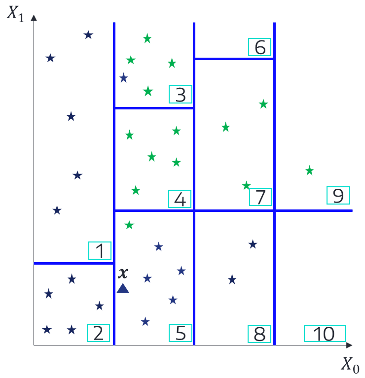
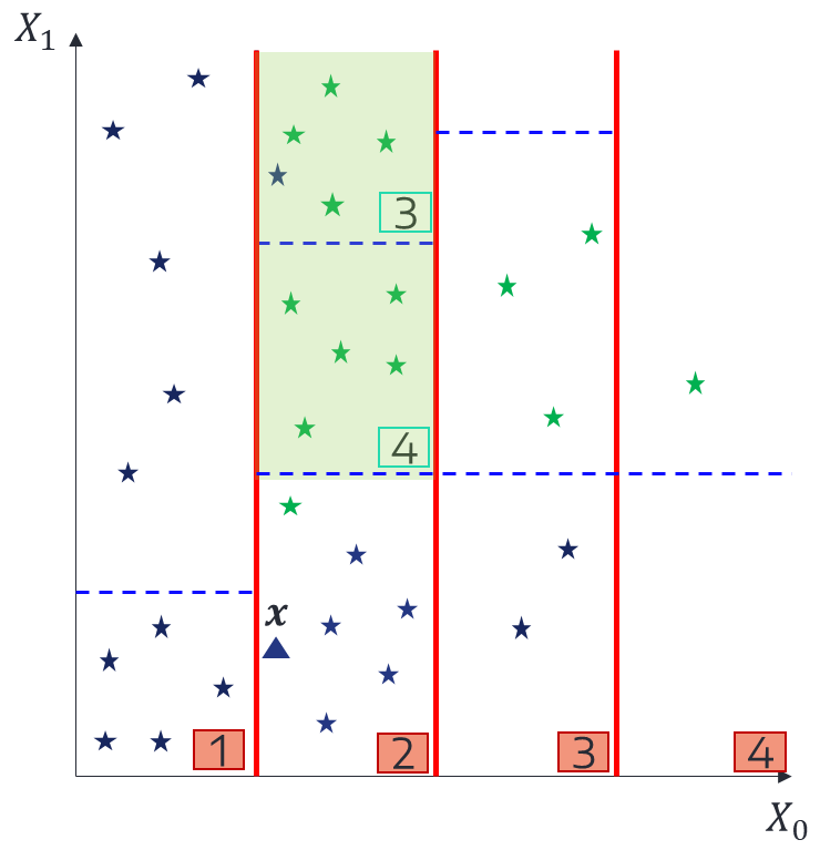
Figure 1: (a) Partition of the RF, (b) Partition of the PRF when we condition on $X_{0}$, i.e., ignoring the splits on $X_{1}$, (c) The optimal CR of $\boldsymbol{x}$ when we condition given $X_{0}=x_{0}$ is the green region.

To illustrate the idea, we use a two-dimensional data $(X_{0},X_{1})$ with label Y represented as green/blue stars in figure 1. We fit a Random Forest to classify this dataset and show its partition in figure 1. The explainee $\boldsymbol{x}$ is the blue triangle. Examining the different cells/leaves of the RF, we deduce that the Minimal Divergent Explanation of $\boldsymbol{x}$ is $S=X_{1}$. In Figure 1, we observe the leaves of the Projected Forest when not conditioning on $S=X_{1}$, thus projecting the RF’s partition only on the subspace $X_{0}$. It consists of ignoring all the splits in the other directions (here the $X_{1}$-axis), thus $\boldsymbol{x}$ falls in the projected leaf 2 (see figure 1) and its $CDP$ is $CDP_{X_{1}}(\text{green};\boldsymbol{x})=\frac{10\text{ green}}{10\text{ green}+17\text{ blue}}=0.58$. To find the optimal rectangle $C_{S}(\boldsymbol{x})=[a_{i},b_{i}]$ in the direction of $X_{1}$, such that the decision changes, we can utilize the leaves of the RF. By looking at the leaves of the RF (figure 1) for observations belonging to the projected RF leaf 2 (Figure 1) where $\boldsymbol{x}$ falls, we observe in Figure 1 that the optimal rectangle for changing the decision, given $X_{0}=x_{0}$ or being in the projected RF leaf 2, is the union of the intervals on $X_{1}$ of the leaf 3 and 4 of the RF (see the green region in Figure 1).

Given an instance $\boldsymbol{x}$ and its Minimal Divergent Explanation $S$, the first step is to collect observations that belong to the leaf of the Projected Forest given $\bar{S}$, where $\boldsymbol{x}$ falls. These observations correspond to those with positive weights in the computation of the $\small CDP_{S}(\boldsymbol{x},\mathscr{Y}^{\star})=\sum_{i=1}^{n}w_{n,i}^{R}(\boldsymbol{x}_{\bar{S}})\mathds{1}_{Y_{i}\in\mathscr{Y}^{\star}}$, i.e., $\small\{\boldsymbol{X}_{i}:w_{n,i}^{R}(\boldsymbol{x}_{\bar{S}})>0\}$. Then, we used the partition of the original forest to find the possible leaves $\small C_{S}(\boldsymbol{x})$ in the direction $S$. The possible leaves is among the RF’s leaves of the collected observations $\small\{\boldsymbol{X}_{i}:w_{n,i}^{R}(\boldsymbol{x}_{\bar{s}})>0\}$. Let denote $\small L(\boldsymbol{X}_{i})$ the leaf of the observation $\boldsymbol{X}_{i}$ with $\small w_{n,i}(\boldsymbol{x}_{\bar{S}})>0$. A possible leaf is a leaf $\small L(\boldsymbol{X}_{i})$ s.t. $\small P(f(\boldsymbol{X})\in\mathscr{Y}^{\star}|\boldsymbol{X}_{S}\in L(\boldsymbol{X}_{i})_{S},\boldsymbol{X}_{\bar{S}}=\boldsymbol{x}_{\bar{S}})\geq\pi_{C}$. Finally, we merge all the possible neighboring leaves to get the largest rectangle, and this maximal rectangle is the counterfactual rule. It is important to note that the union of possible leaves is not necessarily a connected space, which may result in multiple disconnected counterfactual rules.

We apply the same approach to find the regional CR. Given a rule $\boldsymbol{R}$ and its Minimal Divergent Explanation $S$, we used the Projection given $\boldsymbol{X}_{\bar{S}}\in\boldsymbol{R}_{\bar{S}}$ to identify compatible observations and their leaves. We then combine the possible ones that satisfy $CRP_{S}(\boldsymbol{R},\mathscr{Y}^{\star})\geq\pi_{C}$ to obtain the regional CR. For instance, if we consider Leaf 5 of the original forest as a rule (i.e., if $\boldsymbol{X}\in$ Leaf 5, then predict blue), its Minimal Divergent Explanation is also $S=X_{1}$. The Regional CR would be the green region in figure 1. Indeed, satisfying the $X_{0}$ condition of Leaf 5 and the $X_{1}$ condition of Leaves 3 and 4 would cause the decision to change to green.

6 Sampling CE using the CR

Our approaches cannot be directly compared with traditional CE methods, as they return counterfactual samples, whereas we provide rules (ranges of vector values) that permit changing the decision with high probability. In some applications, users might prefer recourse to CR. Hence, we adapt the CR to generate counterfactual samples using a generative model. For example, given an instance $\boldsymbol{x}=(\boldsymbol{x}_{S},\boldsymbol{x}_{\bar{S}})$, target set $\mathscr{Y}^{\star}$ and its counterfactual rule $C_{S}(\boldsymbol{x},\mathscr{Y}^{\star})$, we want to find a sample $x^{\star}=(\boldsymbol{z}_{S},\boldsymbol{x}_{\bar{S}})$ with $\boldsymbol{z}_{S}\in C_{S}(\boldsymbol{x},\mathscr{Y}^{\star})$ s.t $\boldsymbol{x}^{\star}$ is a realistic sample and $f(\boldsymbol{x}^{\star})\in\mathscr{Y}^{\star}$. Instead of using a complex conditional generative model as (Xu et al., 2019; Patki et al., 2016), which can be difficult to calibrate, we use an energy-based generative approach (Grathwohl et al., 2020; Lecun et al., 2006). The core idea is to find $\boldsymbol{z}_{S}\in C_{S}(\boldsymbol{x},\mathscr{Y}^{\star})$ s.t. $\boldsymbol{x}^{\star}$ maximize a given energy score, ensuring that $\boldsymbol{x}^{\star}$ lie in a high-density region. We use the negative outlier score of an Isolation Forest (Liu et al., 2008) and Simulated Annealing (Guilmeau et al., 2021) to maximize the negative outlier score using the information of the counterfactual rules $C_{S}(\boldsymbol{x},\mathscr{Y}^{\star})$. In fact, the range values given by the CR $C_{S}(\boldsymbol{x},\mathscr{Y}^{\star})$ reduce the search space for $\boldsymbol{z}_{S}$ drastically. We used the marginal law of $\boldsymbol{X}$ given $\boldsymbol{X}_{S}\in C_{S}(\boldsymbol{x},\mathscr{Y}^{\star})$ as the proposal distribution, i.e., we draw a candidate $\boldsymbol{z}_{S}$ by independently sampling each variable using the marginal law $\boldsymbol{z}_{S}\sim\prod_{i\in S}P(X_{j}\;|\boldsymbol{X}\in C_{S}(\boldsymbol{x},\mathscr{Y}^{\star})$ until we found an observation $x^{\star}=(\boldsymbol{z}_{S},\boldsymbol{x}_{\bar{S}})$ with a high energy. In practice, we used the training set $\mathcal{D}_{n}$ to find the possible values and we defined $P_{i}$, $P_{S}$ as the list of values of the variable $X_{i}$ found in $\mathcal{D}_{n}$ and $P_{S}=\{\boldsymbol{z}_{S}=(z_{1},\dots,z_{S}):\boldsymbol{z}_{S}\in C_{S}(\boldsymbol{x},\mathscr{Y}^{\star}),z_{i}\in P_{i}\}$ the possible values of $\boldsymbol{X}_{S}$, respectively. Then, we sample $\boldsymbol{z}_{S}$ in the set $P_{S}$ and use Simulated Annealing to find a $\boldsymbol{x}^{\star}=(\boldsymbol{z}_{S},\boldsymbol{x}_{\bar{S}})$ that maximizes the negative outlier score. The algorithm works the same for sampling CE with the Regional CR. A more detailed version of the algorithm is provided in appendix.

7 Experiments

To demonstrate the performance of our framework, we conduct two experiments on real-world datasets. In the first experiment, we showcase the utility of the Local Counterfactual Rules for explaining a regression model. In the second experiment, we compare our approaches with two baseline methods in the context of classification problems: (1) CET (Kanamori et al., 2022), which partition the input space using a decision tree and associate a vector perturbation for each leaf, (2) AReS (Rawal and Lakkaraju, 2020) performs an exhaustive search for finding global counterfactual rules. We used the implementation of Kanamori et al. (2022) that adapts AReS for returning counterfactuals samples instead of rules. We compare the methods only in classification problem as all prior works do not deal with regression problems. In all experiments, we split our dataset into train ($75\%$) - test ($25\%$), and we learn a model $f$, a LightGBM (estimators=50, nb leaves=8), on the train set, which served as the explainee. We learn $f$’s predictions on the train set with an approximating RF (estimators=20, max depth=10): that will be used to generate the CR with $\pi=0.9$. The used parameters for AReS, CET are max rules=8, bins=10 and max iterations=1000, max leaf=8, bins=10 respectively. The other parameters of each method are provided in Appendix.

We evaluate the methods on unseen observations using three metrics. The first metric, Accuracy, measures the average number of instances for which the prescribed action by the methods changes the prediction to the desired outcome. The second metric, Plausibility, measures the average number of inliers (predicted by an Isolation Forest) among the generated counterfactual samples. The third metric, Sparsity, measures the average number of features that have been changed. For the global counterfactual methods (AReS, Regional CR), which do not guarantee to cover all instances, we additionally compute the Coverage, which corresponds to the average number of unseen observations for which they propose a recourse.

Local counterfactual rules for regression. We apply our approach to the California House Price dataset (n=20640, p=8) (Kelley Pace and Barry, 1997), which contains information about each district such as income, population, and location, and the goal is to predict the median house value of each district. To demonstrate the effectiveness of our Local CR method, we focus on a subset of the test set consisting of 1566 houses with prices lower than $100k$. Our objective is to find recourse that would increase their price, such that the price falls within the target range $\mathscr{Y}^{\star}=[200k,250k]$. For each instance $\boldsymbol{x}$, we compute the Minimal Divergent Explanation $S$, the Local CR $C_{S}(\boldsymbol{x},[200k,250k])$, and a generate counterfactula samples using the Simulated Annealing technique described earlier. We succeed in changing the decision for all observations, achieving $\textit{Accuracy}=100\%$. Moreover, the majority of the counterfactual samples passed the outlier test, with a Plausibility score of 0.92. Additionally, our Local CR method achieves a high degree of sparsity, with $\textit{Sparsity}=4.45.$

For instance, the Local CR for the observation $\boldsymbol{x}=$ [Longitude=-118.2, latitude=33.8, housing median age=26, total rooms=703, total bedrooms=202, population=757, households=212, median income=2.52] is $C_{S}(\boldsymbol{x},[200k,250k])=$ [total room $\in[2132,3546],$ total bedrooms $\in[214,491]$] with probability 0.97. This means that if the total number of rooms and total bedrooms satisfy the conditions in $C_{S}(\boldsymbol{x},[200k,250k])$, and the remaining features of $\boldsymbol{x}$ are fixed, then the probability that the price falls within the target set $\mathscr{Y}^{\star}=[200k,250k]$ is 0.97.

Comparisons of Local and Regional CR with baselines (AReS, CET). We evaluate our framework on three real-world datasets: Diabetes (n=768, p=8) (Kaggle, 2016) aims to predict whether a patient has diabetes or not, Breast Cancer Wisconsin (BCW, n=569, p=32) (Dua and Graff, 2017) aims to predict whether a tumor is benign or malignant, and Compas (n=6172, p=12) (Larson et al., 2016) is used to predict criminal recidivism. Our evaluation reveals that AReS and CET are highly sensitive to the number of bins and the maximal number of rules or actions, as previously noted by (Ley et al., 2022). Poor parameterization can result in completely useless explanations. Furthermore, these methods require separate models for each target class, while our framework only requires a single RF with good precision.

Table 1 demonstrates that the Local and Regional CR methods achieve a high level of accuracy in changing decisions on all datasets, surpassing AReS and CET by a significant margin on BCW and Diabetes. Furthermore, the baselines struggle to simultaneously change both the positive and negative classes, e.g., CET has Acc=1 in the positive class, and 0.21 for the negative class on BCW) or when they have a good Acc, the CE are not plausible. For instance, CET has Acc=0.98 and Psb=0 on Compas, meaning that all the counterfactual samples are outliers. Regarding the coverage of the global CE, CET covers all the instances as it partitions the input space, but we observe that AReS has a smaller Coverage$=\{0.43,0.44,0.81\}$ compared to the Regional CR, which has $\{1,0.7,1\}$ for BCW, Diabetes, and Compas respectively.

Noisy responses robustness of Local CR: To assess the robustness of our approach against noisy responses, we conducted an experiment inspired by Pawelczyk et al. (2022). We normalized the datasets so that $\boldsymbol{X}\in[0,1]^{p}$ and added small Gaussian noises $\epsilon$ to the prescribed recourses, with $\epsilon\sim\mathcal{N}(0,\sigma^{2})$, where $\sigma^{2}$ took values of $0.01,0.025,0.05$. We computed the Stability, which is the fraction of unseen instances where the action and perturbed action lead to the same output, for the Compas and Diabetes datasets. We used the simulated annealing approach with the Local CR of section 6 to generate the actions. The Stability metrics for the different noise levels were $0.98,0.98,0.98$ for Compas and $0.96,0.97,0.96$ for Diabetes.

In summary, our CR approach is easier to train, and provides more accurate and plausible rules than the baseline methods. Furthermore, our resulting CE is robust against noisy responses.

Table 1: Results of the Accuracy (Acc), Plausibility, and Sparsity (Sprs) of the different methods. We compute each metric according to the positive (Pos) and negative (Neg) class.

	COMPAS						BCW						Diabetes
	Acc		Psb		Sps		Acc		Psb		Sps		Acc		Psb		Sps
	Pos	Neg	Pos	Neg	Pos	Neg	Pos	Neg	Pos	Neg	Pos	Neg	Pos	Neg	Pos	Neg	Pos	Neg
L-CR	1	0.9	0.87	0.73	2	4	1	1	0.96	1	9	7	0.97	1	0.99	0.8	3	4
R-CR	0.9	0.98	0.74	0.93	2	3	0.89	0.9	0.94	0.93	9	9	0.99	0.99	0.9	0.87	3	4
AReS	0.98	1	0.8	0.61	1	1	0.63	0.34	0.83	0.80	4	3	0.73	0.60	0.77	0.86	1	1
CET	0.85	0.98	0.7	0	2	2	1	0.21	0.6	0.80	8	2	0.84	1	0.60	0.20	6	6

8 Conclusion

We propose a novel approach that formulates CE as Counterfactual Rules. These rules are simple policies that can change the decision of an individual or sub-population with a high probability. Our method is designed to learn robust, plausible, and sparse adversarial regions that indicate where observations should be moved to satisfy a desired outcome. The use of Random Forests is central to our approach, as they provide consistent estimates of interest probabilities and naturally give rise to the counterfactual rules we seek. This also allows us to handle regression problems and continuous features, making our method applicable to a wide range of datasets where tree-based models perform well, such as tabular data.

Appendix A Regional RF detailed

In this section, we give a simple application of the Regional RF algorithm to better understand how it works. Recall that the regional RF is a generalization of the RF’s algorithm to give prediction even when we condition given a region, e.g., to estimate $E(f(\boldsymbol{X})\;|\boldsymbol{X}_{S}\in C_{S}(\boldsymbol{x}),\boldsymbol{X}_{\bar{S}}=\boldsymbol{x}_{\bar{S}})$ with $C_{S}(\boldsymbol{x})=\prod_{i=1}^{|S|}[a_{i},b_{i}],a_{i},b_{i}\in\bar{\mathbb{R}}$ a hyperrectangle. The algorithm works as follows: we drop the observations in the initial trees, if a split used variable $i\in\bar{S}$, a fixed value-based condition, we used the classic rules i.e., if $x_{i}\leq t$, the observations go to the left children, otherwise the right children. However, if a split used variable $i\in S$, regional-based condition, we used the hyperrectangle $C_{S}(\boldsymbol{x})=\prod_{i=1}^{|S|}[a_{i},b_{i}]$. The observations are sent to the left children if $b_{i}\leq t$, right children if $a_{i}>t$ and if $t\in[a_{i},b_{i}]$ the observations are sent both to the left and right children.

To illustrate how it works, we use a two dimensional variables $\boldsymbol{X}\in\mathbb{R}^{2}$, a simple decision tree $f$ represented in figure 2, and want to compute for $\boldsymbol{x}=[1.5,1.9],$ $E(f(\boldsymbol{X})\;|\;\boldsymbol{X}_{1}\in[2,\;3.5],\boldsymbol{X}_{0}=1.5)$. We assume that $P(X_{1}\in[2,\;3.5]\;|\;X_{0}=1.5)>0$ and denoted $T_{1}$ as the set of the values of the splits based on variables $X_{1}$ of the decision tree. One way of estimating this conditional mean is by using Monte Carlo sampling. Therefore, there are two cases :

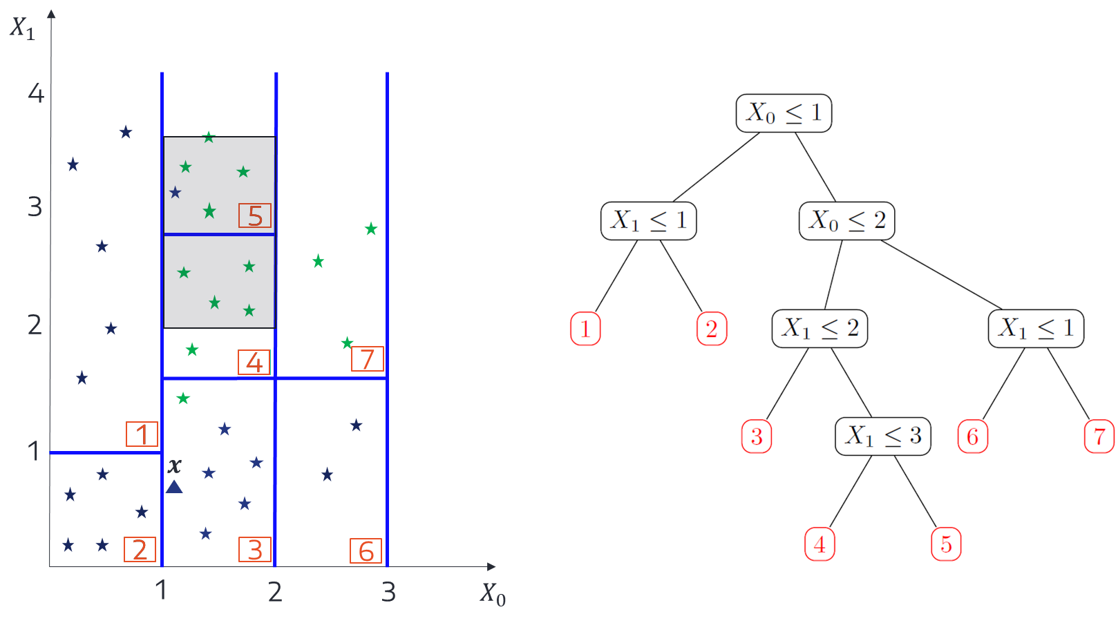
Figure 2: Representation of a simple decision tree (right figure) and its associated partition (left figure). The gray part in the partition corresponds to the region $[2,\;3.5]\times[1,2]$

• If $\forall t\in T_{1},$ $t\leq 2$ or $t>3.5$, then all the observations sampled s.t. $\tilde{X}_{i}\sim P_{\boldsymbol{X}\;|\;\boldsymbol{X}_{1}\in[2,\;3.5],\boldsymbol{X}_{0}=1.5}$ follow the same path and fall in the same leaf. The Monte Carlo estimator of the decision tree $E(f(\boldsymbol{X})|\boldsymbol{X}_{1}\in[2,\;3.5],\boldsymbol{X}_{0}=1.5)$ is equal to the output of the Regional RF algorithm.

  • For instance, a special case of the case above is: if $\forall t\in T_{1},t\leq 2$, and we sample using $P_{\boldsymbol{X}\;|\;\boldsymbol{X}_{1}\in[2,\;3.5],\boldsymbol{X}_{0}=1.5}$, then all the observations go to the right children when they encounters a node using $X_{1}$ and fall in the same leaf.

• If $\exists t\in T_{1}$ and $t\in[2,\;3.5]$, then the observations sampled s.t. $\tilde{X}_{i}\sim P_{\boldsymbol{X}\;|\;\boldsymbol{X}_{1}\in[2,\;3.5],\boldsymbol{X}_{0}=1.5}$ can fall in multiple terminal leaf depending on if their coordinates $x_{1}$ is lower than $t$. Following our example, if we generate samples using $P_{\boldsymbol{X}\;|\;\boldsymbol{X}_{1}\in[2,\;3.5],\boldsymbol{X}_{0}=1.5}$, the observations will fall in the gray region of figure 2, and thus can fall in node 4 or 5. Therefore, the true estimate is:

  $$\small E(f(\boldsymbol{X})|\boldsymbol{X}_{1}\in[2,\;3.5],\boldsymbol{X}_{0}=1.5)=\\ p(X_{1}\leq 2.9\;|X_{0}=1.5)*E[f(\boldsymbol{X})\;|\boldsymbol{X}\in L_{4}]+p(X_{1}>2.9\;|X_{0}=1.5)*E[f(\boldsymbol{X})\;|\boldsymbol{X}\in L_{5}]$$ (1)

Concerning the last case $(t\in[2,\;3.5])$, we need to estimate the different probabilities $p(X_{1}\leq 2.9\;|X_{0}=1.5),p(X_{1}>2.9\;|X_{0}=1.5)$ to compute $E(f(\boldsymbol{X})|\boldsymbol{X}_{1}\in[2,\;3.5],\boldsymbol{X}_{0}=1.5)$, but these probabilities are difficult to estimate in practice. However, we argue that we can ignore these splits, and thus do no need to fragment the query region using the leaves of the tree. Indeed, as we are no longer interest in a point estimate but regional (population mean) we do not need to go to the level of the leaves. We propose to ignore the splits of the leaves that divide the query region. For instance, the leaves 4 and 5 split the region $[2,\;3.5]$ in two cells, by ignoring these splits we estimate the mean of the gray region by taking the average output of the leaves 4 and 5 instead of computing the mean weighted by the probabilities as in eq. 1. Roughly, it consists to follow the classic rules of a decision tree (if the region is above or below a split) and ignore the splits that are in the query region, i.e., we average the output of all the leaves that are compatible with the condition $\boldsymbol{X}_{1}\in[2,\;3.5],\boldsymbol{X}_{0}=1.5$. We think that it leads to a better approximation for two reasons. First, we observe that the case where t is in the region and thus divides the query region does not happen often. Moreover, the leaves of the trees are very small in practice, and taking the mean of the observations that fall in the union of leaves that belong to the query region is more reasonable than computing the weighted mean and thus trying to estimate the different probabilities $p(X_{1}\leq 2.9\;|X_{0}=1.5),p(X_{1}>2.9\;|X_{0}=1.5)$.

Appendix B Additional experiments

In table 2, we compare the Accuracy (Acc), Plausibility (Psb), and Sparsity (Sprs) of the different methods on additonal real-world datasets: FICO [FICO, 2018], NHANESI [CDC, 1999-2022].

We observe that the L-CR, and R-CR outperform the baseline methods by a large margin on Accuracy and Plausibility. The baseline methods still struggle to change at the same time the positive and negative class. In addition, AReS and CET give better sparsity, but their counterfactual samples are less plausible than the ones generated by the CR.

Table 2: Results of the Accuracy (Acc), Plausibility, and Sparsity (Sprs) of the different methods. We compute each metric according to the positive (Pos) and negative (Neg) class.

	FICO						NHANESI
	Acc		Psb		Sps		Acc		Psb		Sps
	Pos	Neg	Pos	Neg	Pos	Neg	Pos	Neg	Pos	Neg	Pos	Neg
L-CR	0.98	0.94	0.98	0.99	5	5	0.99	0.98	0.98	0.97	5	6
R-CR	0.90	0.94	0.98	0.99	9	8.43	0.86	0.95	0.96	0.99	7	7
AReS	0.34	0.01	0.85	0.86	2	1	0.06	1	0.87	0.92	1	1
CET	0.76	0	0.76	0.60	2	2	0	0.40	0.82	0.56	0	5

Appendix C Simulated annealing to generate counterfactual samples using the Counterfactual Rules

⬇

1import numpy as np

2

3def generate_candidate(x, S, x_train, C_S, n_samples):

4 """

5 Generate sample by sampling marginally between the features value of the training observations.

6 Args:

7 x (numpy.ndarray): 1-D array, an observation

8 S (list): contains the indices of the variables on which to condition

9 x_train (numpy.ndarray)): 2-D array represent the training samples

10 C_S (numpy.ndarray)): 3-D (#variables x 2 x 1) representing the hyper-rectangle on which to condition

11 n_samples (int): number of samples

12 Returns:

13The generated samples

14 """

15 x_poss = [x_train[(C_S[i, 0] <= x_train[:, i]) * (x_train[:, i] <= C_S[i, 1]), i] for i in S]

16 x_cand = np.repeat(x.reshape(1, -1), repeats=n_samples, axis=0)

17

18 for i in range(len(S)):

19 rdm_id = np.random.randint(low=0, high=x_poss[i].shape[0], size=n_samples)

20 x_cand[:, S[i]] = x_poss[i][rdm_id]

21

22 return x_cand

23

24

25def simulated_annealing(outlier_score, x, S, x_train, C_S, batch, max_iter, temp, max_iter_convergence):

26 """

27 Generate sample X s.t. X_S \in C_S using simulated annealing and outlier score.

28 Args:

29 outlier_score (lambda functon): outlier_score(X) return a outlier score. If the value are negative, then the observation is an outlier.

30 x (numpy.ndarray)): 1-D array, an observation

31 S (list): contains the indices of the variables on which to condition

32 x_train (numpy.ndarray)): 2-D array represent the training samples

33 C_S (numpy.ndarray)): 3-D (#variables x 2 x 1) representing the hyper-rectangle on which to condition

34 batch (int): number of sample by iteration

35 max_iter (int): number of iteration of the algorithm

36 temp (double): the temperature of the simulated annealing algorithm

37 max_iter_convergence (double): minimun number of iteration to stop the algorithm if it find an in-distribution observation

38

39 Returns:

40 The generated sample, and its outlier score

41 """

42

43 best = generate_candidate(x, S, x_train, C_S, n_samples=1)

44 best_eval = outlier_score(best)[0]

45 curr, curr_eval = best, best_eval

46

47 it = 0

48 for i in range(max_iter):

49

50 x_cand = generate_candidate(curr, S, x_train, C_S, batch)

51 score_candidates = outlier_score(x_cand)

52

53 candidate_eval = np.max(score_candidates)

54 candidate = x_cand[np.argmax(score_candidates)]

55

56 if candidate_eval > best_eval:

57 best, best_eval = candidate, candidate_eval

58 it = 0

59 else:

60 it += 1

61

62 # check convergence

63 if best_eval > 0 and it > max_iter_convergence:

64 break

65

66 diff = candidate_eval - curr_eval

67 t = temp / np.log(float(i + 1))

68 metropolis = np.exp(-diff / t)

69

70 if diff > 0 or rand() < metropolis:

71 curr, curr_eval = candidate, candidate_eval

72

73 return best, best_eval

Listing 1: The simulated annealing algorithm to generate samples that satisfy the condition CR

Appendix D Parameters detailed

In this section, we give the different parameters of each method. For all methods and datasets, we first used a greedy search given a set of parameters. For AReS, we use the following set of parameters:

• max rule = $\{4,6,8\}$, max rule length $=\{4,8\}$, max change num $=\{2,4,6\}$,

• minimal support $=0.05$, discretization bins = $\{10,20\}$,

• $\lambda_{acc}=\lambda_{cov}=\lambda_{cst}=1$.

For CET, we search in the following set of parameters:

• max iterations $=\{500,1000\}$,

• max leaf size $=\{4,6,8,-1\}$,

• $\lambda=0.01,\gamma=1$.

Finally, for the Counterfactual Rules, we used the following parameters:

• nb estimators = $\{20,50\}$, max depth= $\{8,10,12\}$,

• $\pi=0.9$, $\pi_{C}=0.9$.

We obtained the same optimal parameters for all datasets:

• AReS: max rule $=4$, max rule length$=4$, max change num $=4$, minimal support $=0.05$, discretization bins = $10$, $\lambda_{acc}=\lambda_{cov}=\lambda_{cst}=1$

• CET: max iterations $=1000$, max leaf size $=-1$, $\lambda=0.01,\gamma=1$

• CR: nb estimators$=20$, max depth$=10$, $\pi=0.9$, $\pi_{C}=0.9$

References

- Amoukou and Brunel (2021) Salim I Amoukou and Nicolas JB Brunel. Consistent sufficient explanations and minimal local rules for explaining regression and classification models. arXiv preprint arXiv:2111.04658, 2021.
- Basu et al. (2018) Sumanta Basu, Karl Kumbier, James B Brown, and Bin Yu. Iterative random forests to discover predictive and stable high-order interactions. Proceedings of the National Academy of Sciences, 115(8):1943–1948, 2018.
- Bénard et al. (2021a) Clément Bénard, Gérard Biau, Sébastien Da Veiga, and Erwan Scornet. Shaff: Fast and consistent shapley effect estimates via random forests. arXiv preprint arXiv:2105.11724, 2021a.
- Bénard et al. (2021b) Clément Bénard, Gérard Biau, Sébastien Veiga, and Erwan Scornet. Interpretable random forests via rule extraction. In International Conference on Artificial Intelligence and Statistics, pages 937–945. PMLR, 2021b.
- Bénard et al. (2021c) Clément Bénard, Sébastien Da Veiga, and Erwan Scornet. Mda for random forests: inconsistency, and a practical solution via the sobol-mda. arXiv preprint arXiv:2102.13347, 2021c.
- Black et al. (2020) Emily Black, Samuel Yeom, and Matt Fredrikson. Fliptest: fairness testing via optimal transport. In Proceedings of the 2020 Conference on Fairness, Accountability, and Transparency, pages 111–121, 2020.
- Breiman et al. (1984) Leo Breiman, Jerome Friedman, Richard Olshen, and Charles Stone. Classification and regression trees. wadsworth int. Group, 37(15):237–251, 1984.
- CDC (1999-2022) CDC. National health and nutrition examination survey, 1999-2022. URL https://wwwn.cdc.gov/Nchs/Nhanes/Default.aspx.
- Chen et al. (2012) S. Chen, Arthur Choi, and Adnan Darwiche. The same-decision probability: A new tool for decision making. 2012.
- Chou et al. (2022) Yu-Liang Chou, Catarina Moreira, Peter Bruza, Chun Ouyang, and Joaquim Jorge. Counterfactuals and causability in explainable artificial intelligence: Theory, algorithms, and applications. Information Fusion, 81:59–83, 2022. ISSN 1566-2535. doi: https://doi.org/10.1016/j.inffus.2021.11.003. URL https://www.sciencedirect.com/science/article/pii/S1566253521002281.
- De Lara et al. (2021) Lucas De Lara, Alberto González-Sanz, Nicholas Asher, and Jean-Michel Loubes. Transport-based counterfactual models. arXiv preprint arXiv:2108.13025, 2021.
- Du et al. (2021) Qiming Du, Gérard Biau, François Petit, and Raphaël Porcher. Wasserstein random forests and applications in heterogeneous treatment effects. In International Conference on Artificial Intelligence and Statistics, pages 1729–1737. PMLR, 2021.
- Dua and Graff (2017) Dheeru Dua and Casey Graff. UCI machine learning repository, 2017. URL http://archive.ics.uci.edu/ml.
- FICO (2018) FICO. Fico. explainable machine learning challenge, 2018. URL https://community.fico.com/s/explainable-machine-learning-challenge.
- Grathwohl et al. (2020) Will Grathwohl, Kuan-Chieh Wang, Joern-Henrik Jacobsen, David Duvenaud, Mohammad Norouzi, and Kevin Swersky. Your classifier is secretly an energy based model and you should treat it like one. In International Conference on Learning Representations, 2020.
- Grinsztajn et al. (2022) Leo Grinsztajn, Edouard Oyallon, and Gael Varoquaux. Why do tree-based models still outperform deep learning on typical tabular data? In Thirty-sixth Conference on Neural Information Processing Systems Datasets and Benchmarks Track, 2022.
- Guilmeau et al. (2021) Thomas Guilmeau, Emilie Chouzenoux, and Víctor Elvira. Simulated annealing: a review and a new scheme. pages 101–105, 07 2021. doi: 10.1109/SSP49050.2021.9513782.
- Ishwaran et al. (2008) Hemant Ishwaran, Udaya B Kogalur, Eugene H Blackstone, and Michael S Lauer. Random survival forests. The annals of applied statistics, 2(3):841–860, 2008.
- Kaggle (2016) Kaggle. Pima indians diabetes database, 2016. URL https://www.kaggle.com/datasets/uciml/pima-indians-diabetes-database.
- Kanamori et al. (2020) Kentaro Kanamori, Takuya Takagi, Ken Kobayashi, and Hiroki Arimura. Dace: Distribution-aware counterfactual explanation by mixed-integer linear optimization. In IJCAI, 2020.
- Kanamori et al. (2022) Kentaro Kanamori, Takuya Takagi, Ken Kobayashi, and Yuichi Ike. Counterfactual explanation trees: Transparent and consistent actionable recourse with decision trees. In Proceedings of The 25th International Conference on Artificial Intelligence and Statistics, PMLR 151:1846-1870, 2022.
- Karimi et al. (2020a) Amir-Hossein Karimi, Gilles Barthe, Borja Balle, and Isabel Valera. Model-agnostic counterfactual explanations for consequential decisions. ArXiv, abs/1905.11190, 2020a.
- Karimi et al. (2020b) Amir-Hossein Karimi, Gilles Barthe, Bernhard Schölkopf, and Isabel Valera. A survey of algorithmic recourse: definitions, formulations, solutions, and prospects. CoRR, abs/2010.04050, 2020b. URL https://arxiv.org/abs/2010.04050.
- Kelley Pace and Barry (1997) R. Kelley Pace and Ronald Barry. Sparse spatial autoregressions. Statistics, Probability Letters, 33(3):291–297, 1997. ISSN 0167-7152. doi: https://doi.org/10.1016/S0167-7152(96)00140-X. URL https://www.sciencedirect.com/science/article/pii/S016771529600140X.
- Lakkaraju et al. (2022) Himabindu Lakkaraju, Dylan Slack, Yuxin Chen, Chenhao Tan, and Sameer Singh. Rethinking explainability as a dialogue: A practitioner’s perspective. CoRR, abs/2202.01875, 2022. URL https://arxiv.org/abs/2202.01875.
- Larson et al. (2016) Jeff Larson, Surya Mattu, Lauren Kirchner, , and Julia Angwin. How we analyzed the compas recidivism algorithm, 2016. URL https://www.propublica.org/article/how-we-analyzed-the-compas-recidivism-algorithm.
- Lecun et al. (2006) Yann Lecun, Sumit Chopra, and Raia Hadsell. A tutorial on energy-based learning. 01 2006.
- Ley et al. (2022) Dan Ley, Saumitra Mishra, and Daniele Magazzeni. Global counterfactual explanations: Investigations, implementations and improvements, 2022. URL https://arxiv.org/abs/2204.06917.
- Liu et al. (2008) Fei Tony Liu, Kai Ming Ting, and Zhi-Hua Zhou. Isolation forest. In 2008 eighth ieee international conference on data mining, pages 413–422. IEEE, 2008.
- Loh (2011) Wei-Yin Loh. Classification and regression trees. Wiley Interdisciplinary Reviews: Data Mining and Knowledge Discovery, 1, 2011.
- Looveren and Klaise (2019) Arnaud Van Looveren and Janis Klaise. Interpretable counterfactual explanations guided by prototypes. CoRR, abs/1907.02584, 2019. URL http://arxiv.org/abs/1907.02584.
- Lundberg et al. (2020) Scott M. Lundberg, Gabriel Erion, Hugh Chen, Alex DeGrave, Jordan M. Prutkin, Bala Nair, Ronit Katz, Jonathan Himmelfarb, Nisha Bansal, and Su-In Lee. From local explanations to global understanding with explainable ai for trees. Nature Machine Intelligence, 2(1):2522–5839, 2020.
- Meinshausen and Ridgeway (2006) Nicolai Meinshausen and Greg Ridgeway. Quantile regression forests. Journal of Machine Learning Research, 7(6), 2006.
- Molnar (2022) Christoph Molnar. Interpretable Machine Learning. 2 edition, 2022. URL https://christophm.github.io/interpretable-ml-book.
- Mothilal et al. (2020) Ramaravind K. Mothilal, Amit Sharma, and Chenhao Tan. Explaining machine learning classifiers through diverse counterfactual explanations. In Proceedings of the 2020 Conference on Fairness, Accountability, and Transparency, FAT* ’20, page 607–617, New York, NY, USA, 2020. Association for Computing Machinery. ISBN 9781450369367. doi: 10.1145/3351095.3372850. URL https://doi.org/10.1145/3351095.3372850.
- Parmentier and Vidal (2021) Axel Parmentier and Thibaut Vidal. Optimal counterfactual explanations in tree ensembles. CoRR, abs/2106.06631, 2021. URL https://arxiv.org/abs/2106.06631.
- Patki et al. (2016) N. Patki, R. Wedge, and K. Veeramachaneni. The synthetic data vault. In 2016 IEEE International Conference on Data Science and Advanced Analytics (DSAA), pages 399–410, Oct 2016. doi: 10.1109/DSAA.2016.49.
- Pawelczyk et al. (2022) Martin Pawelczyk, Teresa Datta, Johannes van-den Heuvel, Gjergji Kasneci, and Himabindu Lakkaraju. Algorithmic recourse in the face of noisy human responses, 2022. URL https://arxiv.org/abs/2203.06768.
- Poyiadzi et al. (2019) Rafael Poyiadzi, Kacper Sokol, Raúl Santos-Rodriguez, Tijl De Bie, and Peter A. Flach. FACE: feasible and actionable counterfactual explanations. CoRR, abs/1909.09369, 2019. URL http://arxiv.org/abs/1909.09369.
- Rawal and Lakkaraju (2020) Kaivalya Rawal and Himabindu Lakkaraju. Beyond individualized recourse: Interpretable and interactive summaries of actionable recourses. Advances in Neural Information Processing Systems, 33:12187–12198, 2020.
- Ribeiro et al. (2016) Marco Tulio Ribeiro, Sameer Singh, and Carlos Guestrin. " why should i trust you?" explaining the predictions of any classifier. In Proceedings of the 22nd ACM SIGKDD international conference on knowledge discovery and data mining, pages 1135–1144, 2016.
- Russell (2019) Chris Russell. Efficient search for diverse coherent explanations. In Proceedings of the Conference on Fairness, Accountability, and Transparency, FAT* ’19, page 20–28, New York, NY, USA, 2019. Association for Computing Machinery. ISBN 9781450361255. doi: 10.1145/3287560.3287569. URL https://doi.org/10.1145/3287560.3287569.
- Ustun et al. (2019) Berk Ustun, Alexander Spangher, and Yang Liu. Actionable recourse in linear classification. Proceedings of the Conference on Fairness, Accountability, and Transparency, 2019.
- Verma et al. (2020) Sahil Verma, John P. Dickerson, and Keegan Hines. Counterfactual explanations for machine learning: A review. CoRR, abs/2010.10596, 2020. URL https://arxiv.org/abs/2010.10596.
- Wachter et al. (2017) Sandra Wachter, Brent Daniel Mittelstadt, and Chris Russell. Counterfactual explanations without opening the black box: Automated decisions and the gdpr. Cybersecurity, 2017.
- Wager and Athey (2017) Stefan Wager and Susan Athey. Estimation and inference of heterogeneous treatment effects using random forests, 2017.
- Xu et al. (2019) Lei Xu, Maria Skoularidou, Alfredo Cuesta-Infante, and Kalyan Veeramachaneni. Modeling tabular data using conditional gan. In NeurIPS, 2019.
Supplementary Materials