Phase function methods for second order linear ordinary differential equations with turning points

Abstract

It is well known that second order linear ordinary differential equations with slowly varying coefficients admit slowly varying phase functions. This observation is the basis of the Liouville-Green method and many other techniques for the asymptotic approximation of the solutions of such equations. More recently, it was exploited by the author to develop a highly efficient solver for second order linear ordinary differential equations whose solutions are oscillatory. In many cases of interest, that algorithm achieves near optimal accuracy in time independent of the frequency of oscillation of the solutions. Here we show that, after minor modifications, it also allows for the efficient solution of second order differential equations which have turning points. That is, it is effective in the case of equations whose solutions are oscillatory in some regions and behave like linear combinations of increasing and decreasing exponential functions in others. We present the results of numerical experiments demonstrating the properties of our method, including some which show that it can used to evaluate many classical special functions in time independent of the parameters on which they depend.

Abstract

It is well known that second order linear ordinary differential equations with slowly varying coefficients admit slowly varying phase functions. This observation is the basis of the Liouville-Green method and many other techniques for the asymptotic approximation of the solutions of such equations. More recently, it was exploited by the author to develop a highly efficient solver for second order linear ordinary differential equations whose solutions are oscillatory. In many cases of interest, that algorithm achieves near optimal accuracy in time independent of the frequency of oscillation of the solutions. Here we show that, after minor modifications, it also allows for the efficient solution of second order differential equations which have turning points. That is, it is effective in the case of equations whose solutions are oscillatory in some regions and behave like linear combinations of increasing and decreasing exponential functions in others. We present the results of numerical experiments demonstrating the properties of our method, including some which show that it can used to evaluate many classical special functions in time independent of the parameters on which they depend. ordinary differential equations; fast algorithms; special functions.

1 Introduction

It has long been known that the solutions of second order linear ordinary differential equations with slowly varying coefficients can be approximated via slowly varying phase functions. This principle is the basis of many asymptotic techniques, including the venerable Liouville-Green method. If $q$ is smooth and strictly positive on the interval $[a,b]$, then

$$u_{0}(t)=\frac{\cos\left(\alpha_{0}(t)\right)}{\sqrt{\alpha_{0}^{\prime}(t)}}\ \ \mbox{and}\ \ \ v_{0}(t)=\frac{\sin\left(\alpha_{0}(t)\right)}{\sqrt{\alpha_{0}^{\prime}(t)}},$$ (1)

where $\alpha_{0}$ is defined via

$$\alpha_{0}(t)=\int_{a}^{t}\sqrt{q(s)}\ ds,$$ (2)

are a pair of Liouville-Green approximates for the second order linear ordinary differential equation

$$y^{\prime\prime}(t)+q(t)y(t)=0,\ \ a<t<b.$$ (3)

When $q$ is slowly varying, so too is the function defined via (2), and this is the case regardless of the magnitude of $q$. By contrast, the solutions of (3) become increasing oscillatory as $q$ grows in magnitude. For a careful discussion of the Liouville-Green method, including rigorous error bounds for the approximates (1), we refer the reader to Chapter 6 of [16].

If $\alpha$ is a phase function for (3) — so that

$$u(t)=\frac{\cos\left(\alpha(t)\right)}{\sqrt{\alpha^{\prime}(t)}}\ \ \mbox{and}\ \ \ v(t)=\frac{\sin\left(\alpha(t)\right)}{\sqrt{\alpha^{\prime}(t)}}$$ (4)

are solutions of (3) — then $\alpha^{\prime}$ satisfies Kummer’s differential equation

$$q(t)-(\alpha^{\prime}(t))^{2}+\frac{3}{4}\left(\frac{\alpha^{\prime\prime}(t)}{\alpha^{\prime}(t)}\right)^{2}-\frac{\alpha^{\prime\prime\prime}(t)}{2\alpha^{\prime}(t)}=0,\ \ a<t<b.$$ (5)

The Liouville-Green phase (2) is the (crude) approximation obtained by deleting the expression

$$\frac{3}{4}\left(\frac{\alpha^{\prime\prime}(t)}{\alpha^{\prime}(t)}\right)^{2}-\frac{\alpha^{\prime\prime\prime}(t)}{2\alpha^{\prime}(t)}=0$$ (6)

from (5) and solving the resulting equation. In [18], an iterative scheme for refining the Liouville-Green phase is introduced. In order to avoid the complications which square roots bring, it constructs a sequence $\phi_{0},\phi_{1},\phi_{2},\ldots$ of asymptotic approximations to a solution of the differential equation

$$\phi(t)=q(t)-\frac{1}{4}\frac{\phi^{\prime\prime}(t)}{\phi(t)}+\frac{5}{16}\left(\frac{\phi^{\prime}(t)}{\phi(t)}\right)^{2}$$ (7)

satisfied by functions of the form $\phi(t)=\left(\alpha^{\prime}(t)\right)^{2}$, where $\alpha^{\prime}$ is the derivative of a phase function for (3). The formulas

$$\left\{\begin{aligned} \phi_{0}(t)&=q(t)\\ \phi_{n+1}(t)&=q(t)-\frac{1}{4}\frac{\phi_{n}^{\prime\prime}(t)}{\phi_{n}(t)}+\frac{5}{16}\left(\frac{\phi_{n}^{\prime}(t)}{\phi_{n}(t)}\right)^{2}\end{aligned}\right.$$ (8)

defining the scheme of [18] make clear that when $q$ and its derivatives are slowly varying, the asymptotic approximations it produces will be as well. Error bounds which hold under various assumptions on the form of $q$ are given in [19, 17, 18]. In the important case in which

$$q(t)=\lambda^{2}q_{0}(t)$$ (9)

with $q_{0}$ smooth and positive, there exist solutions $u$, $v$ of (3) such that if $\alpha_{n}$ is the approximate phase function obtained from the iterate $\phi_{n}$ of the scheme (8), then

$$u(t) =\frac{\cos\left(\alpha_{n}(t)\right)}{\sqrt{\alpha_{n}^{\prime}(t)}}+\mathcal{O}\left(\frac{1}{\lambda^{n+1}}\right)\ \ \mbox{as}\ \ \lambda\to\infty\ \ \mbox{and}$$ (10)

$$v(t) =\frac{\sin\left(\alpha_{n}(t)\right)}{\sqrt{\alpha_{n}^{\prime}(t)}}+\mathcal{O}\left(\frac{1}{\lambda^{n+1}}\right)\ \ \mbox{as}\ \ \lambda\to\infty.$$

The approximations generated by the scheme of [18] are closely connected to the (perhaps more familiar) classical ones obtained from the Riccati equation

$$r^{\prime}(t)+(r(t))^{2}+q(t)=0$$ (11)

satisfied by the logarithmic derivatives of the solutions of (3). We note that the solutions of (11) are related to those of (5) via the formula

$$r(t)=i\alpha^{\prime}(t)-\frac{1}{2}\frac{\alpha^{\prime\prime}(t)}{\alpha^{\prime}(t)}.$$ (12)

In the event that $q$ takes the form (9), inserting the ansatz

$$r(t)=\sum_{k=0}^{n}\lambda^{1-k}r_{k}(t)$$ (13)

into (11) and solving the equations which result from collecting like powers of $\lambda$ leads to the formulas

$$r_{0}(t) =i\sqrt{q_{0}(t)},$$ (14)

$$r_{1}(t) =-\frac{q_{0}^{\prime}(t)}{4q_{0}(t)},$$

$$\vdots$$

$$r_{n}(t) =-\frac{i}{2\sqrt{q_{0}(t)}}\left(r_{n-1}^{\prime}(t)+\sum_{j=0}^{n-1}r_{j}(t)r_{n-j}(t)\right).$$

It is a classical result (a proof of which can be found in Chapter 7 of [15]) that there exist solutions $u$, $v$ of (3) such that

$$u(t) =\exp\left(i\sum_{n=0}^{n}\lambda^{1-n}\int_{a}^{t}r_{n}(s)\ ds\right)+\mathcal{O}\left(\frac{1}{\lambda^{n+1}}\right)\ \ \mbox{as}\ \ \lambda\to\infty\ \ \mbox{and}$$ (15)

$$v(t) =\exp\left(-i\sum_{n=0}^{n}\lambda^{1-n}\int_{a}^{t}r_{n}(s)\ ds\right)+\mathcal{O}\left(\frac{1}{\lambda^{n+1}}\right)\ \ \mbox{as}\ \ \lambda\to\infty.$$

Since the formula defining $r_{n+1}$ depends on all of the previous iterates $r_{0},r_{1},\ldots,r_{n}$ whereas the $(n+1)^{st}$ iterate $\phi_{n+1}$ depends only on the $n^{th}$ iterate $\phi_{n}$, the approximations produced by the scheme (8) are typically much simpler than those which result from the classical scheme.

While asymptotic methods such as (8) and (13), (14) are extremely useful for generating symbolic expressions which represent the solutions of second order linear ordinary differential equations, they leave much to be desired as numerical methods. Such schemes suffer from at least two serious problems:

1. Like all asymptotic methods, there is a limit to the accuracy which they can obtain, and this limit often falls short of the level of accuracy indicated by the condition number of the problem. Moreover, in the case of asymptotic methods for (3), the obtainable accuracy generally depends in a complicated way on behavior of the function $q$ and its derivatives, thus making it difficult to control numerical errors.

2. The higher order approximations constructed by these techniques depend on higher order derivatives of $q$, which cannot be calculated numerically without significant loss of accuracy.

In [7], an algorithm for constructing nonoscillatory phase functions which represent the solutions of equations of the form (3) when $q$ is smooth and strictly positive is described. It operates by solving Kummer’s equation (5) numerically. Most of the solutions of Kummer’s equation are oscillatory, and the principal challenge addressed by the algorithm of [7] is the identification of the values of the first two derivatives of a nonoscillatory phase function at a point on the interval $(a,b)$. Once this has been done, (5) can be solved numerically using any method which applies to stiff ordinary differential equations. The algorithm of [7] does not require knowledge of the derivatives of $q$ and calculates the phase function $\alpha$ to near machine precision regardless of the magnitude of $q$.

A theorem which shows the existence of a nonoscillatory phase function for (3) in the case in which $q$ is of the form (9) appears in a companion paper [9] to [7]. It applies when the function $p(x)=\widetilde{p}(t(x))$, where $p(t)$ is defined via

$$\widetilde{p}(t)=\frac{1}{q_{0}(t)}\left(\frac{5}{4}\left(\frac{q_{0}^{\prime}(t)}{q_{0}(t)}\right)^{2}-\frac{q_{0}^{\prime\prime}(t)}{q_{0}(t)}\right)=4\left(q_{0}(t)\right)^{\frac{1}{4}}\frac{d}{dt}\left(\frac{1}{\left(q_{0}(t)\right)^{\frac{1}{4}}}\right)$$ (16)

and $t(x)$ is the inverse function of

$$x(t)=\int_{a}^{t}\sqrt{q_{0}(s)}\ ds,$$ (17)

has a rapidly decaying Fourier transform. More explicitly, the theorem asserts that if the Fourier transform of $p$ satisfies a bound of the form

$$\left|\widehat{p}(\xi)\right|\leq\Gamma\exp\left(-\mu\left|\xi\right|\right),$$ (18)

then there exist functions $\nu$ and $\delta$ such that

$$\left|\nu(t)\right|\leq\frac{\Gamma}{2\mu}\left(1+\frac{4\Gamma}{\lambda}\right)\exp(-\mu\lambda),$$ (19)

$$\left|\widehat{\delta}(\xi)\right|\leq\frac{\Gamma}{\lambda^{2}}\left(1+\frac{2\Gamma}{\lambda}\right)\exp(-\mu|\xi|)$$ (20)

and

$$\alpha(t)=\lambda\sqrt{q_{0}(t)}\int_{a}^{t}\exp\left(\frac{\delta(u)}{2}\right)\ du$$ (21)

is a phase function for

$$y^{\prime\prime}(t)+\lambda^{2}\left(q_{0}(t)+\frac{\nu(t)}{4\lambda^{2}}\right)y(t)=0.$$ (22)

The definition of the function $p(x)$ is ostensibly quite complicated; however, $p(x)$ is, in fact, simply equal to twice the Schwarzian derivative of the inverse function $t(x)$ of (17). This theorem ensures that, even for relatively modest values of $\lambda$, the phase function constructed by [7] is nonoscillatory. When $\lambda$ is small, the algorithm of [7] is not guaranteed to produce a phase function which is nonoscillatory, but, in stark contrast to asymptotic methods, in all cases it results in one which approximates a solution of (5) with near machine precision accuracy.

Here, we describe a variant of the algorithm of [7] which allows for the numerical solution of second order linear ordinary differential equations with turning points. We focus on the case in which the coefficient $q$ in (3) is a smooth function on the interval $(a,b)$ with a single zero at the point $c\in(a,b)$, and further assume that

$$q(t)\sim C(t-c)^{k}\ \ \mbox{as}\ \ t\to c$$ (23)

with $k$ a positive integer. Most equations with multiple turning points can be handled by the repeated use of the algorithm described here (and we consider two such examples in the numerical experiments discussed in this article). When $q$ is nonpositive on the entire interval $(a,b)$, alternate methods are indicated (for example, the technique used in [8] to solve second order differential equations in the nonoscillatory regime).

Two problems arise when the algorithm of [7] is applied to second order differential equations of this type. First, Kummer’s equation (5) and the closely-related Riccati equation (11) encounter numerical difficulties in the nonoscillatory regime, where the values of $\alpha^{\prime}$ are small. More explicitly, when these equations are solved numerically, the obtained values of $\alpha^{\prime}$ only approximate it with absolute accuracy on the order of machine precision in the nonoscillatory region. Since $\alpha^{\prime}$ is small there, this means that the relative accuracy of these approximations is extremely poor. That such difficulties are encountered is unsurprising given that $\alpha^{\prime}$ appears in the denominator of two terms in Kummer’s equation, and considering the form (9) of the solutions of Riccati’s equation. We address this difficulty by solving Appell’s equation rather than Kummer’s equation. Appell’s equation is a certain third order linear ordinary differential equation satisfied by the product of any two solutions of (3), including the reciprocal of $\alpha^{\prime}$, which is the sum of the squares of the two functions appearing in (4). As the experiments discussed in this paper show, there is no difficulty in calculating $\alpha^{\prime}$ with high relative accuracy in both the oscillatory and nonoscillatory regimes by solving Appell’s equation numerically.

The second difficulty addressed by the algorithm of this paper is that, in the case of turning points of even orders, there need not exist a slowly varying phase function which extends across the turning point. We include a simple analysis of the second order differential equation

$$y^{\prime\prime}(t)+t^{k}y(t)=0$$ (24)

in the case in which $k$ is an even integer to demonstrate this. To overcome this problem, we simply construct two nonoscillatory phase functions, each defined only on one side of the turning point. For turning points of odd order, a single phase function suffices.

The remainder of this article is structured as follows. Section 2 reviews certain basic facts regarding phase functions for second order linear ordinary differential equations. In Section 3, we analyze the second order differential equation (24) in order to show that we cannot expect nonoscillatory phase functions to extend across turning points of even order. Section 4 details our numerical algorithm. Numerical experiments conducted to demonstrate its properties are discussed in Section 5. We close with a few brief remarks in Section 6.

2 Phase functions for second order linear ordinary differential equations

In this section, we review several basic facts regarding phase functions for second order linear ordinary differential equations. We first discuss the case of a general second order linear ordinary differential equation in Subsection 2.1, and then we consider the effect of applying the standard transform which reduces such equations to their so-called “normal forms” in Subsection 2.2.

2.1 The general case

If $y(t)=\exp(r(t))$ satisfies the second order differential equation

$$y^{\prime\prime}(t)+p(t)y^{\prime}(t)+q(t)y(t)=0,\ \ a<t<b,$$ (25)

then it can be easily seen that r(t) solves the Riccati equation

$$r^{\prime\prime}(t)+(r^{\prime}(t))^{2}+p(t)r^{\prime}(t)+q(t)=0,\ \ a<t<b.$$ (26)

Letting $r(t)=i\alpha(t)+\beta(t)$ yields the system of ordinary differential equations

$$\left\{\begin{aligned} q(t)-(\alpha^{\prime}(t))^{2}+p(t)\beta^{\prime}(t)+(\beta^{\prime}(t))^{2}+\beta^{\prime\prime}(t)&=0\\ p(t)\alpha^{\prime}(t)+2\alpha^{\prime}(t)\beta^{\prime}(t)+\alpha^{\prime\prime}(t)&=0.\end{aligned}\right.$$ (27)

The second of these can be rearranged as

$$\beta^{\prime}(t)=-\frac{1}{2}\frac{\alpha^{\prime\prime}(t)}{\alpha^{\prime}(t)}-\frac{p(t)}{2},$$ (28)

and when this expression is inserted into the first equation in (27) we arrive at

$$q(t)-\frac{(p(t))^{2}}{4}-\frac{p^{\prime}(t)}{2}-(\alpha^{\prime}(t))^{2}+\frac{3}{4}\left(\frac{\alpha^{\prime\prime}(t)}{\alpha^{\prime}(t)}\right)^{2}-\frac{\alpha^{\prime\prime\prime}(t)}{2\alpha^{\prime}(t)}=0,\ \ a<t<b.$$ (29)

It is clear that if $\alpha$ does not vanish on $(a,b)$ and satisfies (29) there, then

$$r(t)=i\alpha(t)-\frac{1}{2}\log\left(\alpha^{\prime}(t)\right)-\int p(t)\ dt,$$ (30)

where the implicit constant of integration and the choice of branch cut for the logarithm are irrelevant, is a solution of the Riccati equation (26) and

$$\sqrt{\frac{\omega(t)}{\alpha^{\prime}(t)}}\exp(i\alpha(t))=\sqrt{\frac{\omega(t)}{\alpha^{\prime}(t)}}\cos(\alpha(t))+i\sqrt{\frac{\omega(t)}{\alpha^{\prime}(t)}}\sin(\alpha(t)),$$ (31)

where

$$\omega(t)=\exp\left(-\int p(t)\ dt\right),$$ (32)

is a solution of the original ordinary differential equation (25). We note that Abel’s identity implies that the Wronskian of any pair of solutions of (25) is a constant multiple of (32).

Equation (29) is known as Kummer’s equation, after E. E. Kummer who considered it in [14] and we refer to its solutions as phase functions for the ordinary differential equation (25). When the coefficients $p$ and $q$ are real-valued, $\alpha(t)$ is also real-valued, and the functions

$$u(t)=\sqrt{\frac{\omega(t)}{\alpha^{\prime}(t)}}\cos(\alpha(t))\ \ \mbox{and}\ \ \ v(t)=\sqrt{\frac{\omega(t)}{\alpha^{\prime}(t)}}\sin(\alpha(t))$$ (33)

are linearly independent real-valued solutions of (25) which form a basis in its space of solutions.

If $\alpha$ is a phase function and $u$ and $v$ are as in (33), then a straightforward computation shows that the modulus function

$$m(t)=(u(t))^{2}+(v(t))^{2}=\frac{\omega(t)}{\alpha^{\prime}(t)}$$ (34)

satisfies the differential equation

$$m^{\prime\prime\prime}(t)+3p(t)m^{\prime\prime}(t)+(2(p(t))^{2}+p^{\prime}(t)+4q(t))m^{\prime}(t)+(4p(t)q(t)+2q^{\prime}(t))m(t)=0.$$ (35)

We refer to (35) as Appell’s equation in light of the article [1].

Given any pair $u,v$ of solutions of (25) whose Wronskian $\omega(t)$ and the associated modulus function $m(t)=(u(t))^{2}+(v(t))^{2}$ are nonzero on $(a,b)$, it can be shown by a straightforward calculation that

$$\alpha^{\prime}(t)=\frac{\omega(t)}{(u(t))^{2}+(v(t))^{2}}$$ (36)

satisfies (29) on that interval. It follows that any antiderivative of $\alpha^{\prime}$ is a phase function for (25) on $(a,b)$. Requiring that (33) holds determines $\alpha$ up to an additive constant which is an integral multiple of $2\pi$, but further restrictions are required to determine it uniquely. We will nonetheless, by a slight abuse of terminology, refer to “the phase function generated by the pair of solutions $u,v$” with the understanding that the choice of constant is of no consequence.

2.2 Reduction to normal form

If $y$ solves (25), then

$$\tilde{y}(t)=\exp\left(-\frac{1}{2}\int p(t)\ dt\right)y(t)$$ (37)

satisfies

$$\tilde{y}^{\prime\prime}(t)+\tilde{q}(t)\tilde{y}(t)=0,\ \ a<t<b,$$ (38)

where

$$\tilde{q}(t)=q(t)-\frac{p(t)}{2}-\frac{(p(t))^{2}}{4}.$$ (39)

Equation (38) is often called the normal form of (25). The effects of this transformation on the various formulas discussed above are easy to discern. In particular, Riccati’s equation becomes

$$\tilde{r}^{\prime\prime}(t)+(\tilde{r}^{\prime}(t))^{2}+\tilde{q}(t)=0,$$ (40)

Kummer’s equation now takes the form

$$\tilde{q}(t)-(\tilde{\alpha}^{\prime}(t))^{2}+\frac{3}{4}\left(\frac{\tilde{\alpha}^{\prime\prime}(t)}{\tilde{\alpha}^{\prime}(t)}\right)^{2}-\frac{\tilde{\alpha}^{\prime\prime\prime}(t)}{2\tilde{\alpha}^{\prime}(t)}=0,\ \ a<t<b,$$ (41)

Appell’s equation becomes

$$\tilde{m}^{\prime\prime\prime}(t)+4\tilde{q}(t)\tilde{m}^{\prime}(t)+2\tilde{q}^{\prime}(t)\tilde{m}(t)=0,$$ (42)

and it is the functions

$$\tilde{u}(t)=\frac{\cos(\tilde{\alpha}(t))}{\sqrt{\tilde{\alpha}^{\prime}(t)}}\ \ \mbox{and}\ \ \ \tilde{v}(t)=\frac{\sin(\tilde{\alpha}(t))}{\sqrt{\tilde{\alpha}^{\prime}(t)}}$$ (43)

which form a basis in the space of solutions of (38).

We observe that when (39) is inserted into (41) it simply becomes (29), so that Kummer’s equation is unchanged by this transformation. Similarly, (36) is invariant under (37), which implies that

$$\alpha^{\prime}(t)=\tilde{\alpha}^{\prime}(t).$$ (44)

So while the solution of Riccati’s equation and the basis functions are modified by the transformation (37), the phase function $\alpha$ is invariant. It does not matter, then, whether the form (25) or its normal form (38) is considered. Either set of solutions (33) or (43) can be recovered once $\alpha$ has been calculated.

3 Turning points of even order

We now consider the equation

$$y^{\prime\prime}(t)+t^{k}y(t)=0$$ (45)

in the case in which $k$ is an even integer. Since the solutions of (45) can be expressed as linear combinations of Bessel functions, we begin with a short discussions of Bessel’s differential equation in Subsection 3.1. We then exhibit a basis in the space of solutions of (45) in Subsection 3.2. Finally, in Subsection 3.3, we show that (45) does not admit a phase function which is nonoscillatory on all of the real line.

3.1 Bessel functions

Standard solutions of Bessel’s differential equation

$$z^{2}y^{\prime\prime}(z)+zy^{\prime}(z)+(z^{2}-\nu^{2})y(z)=0$$ (46)

include the Bessel functions

$$J_{\nu}(z)=\left(\frac{z}{2}\right)^{\nu}\sum_{k=0}^{\infty}\frac{1}{\Gamma(k+1)\Gamma(k+\nu+1)}\left(\frac{z}{2}\right)^{k}$$ (47)

and

$$Y_{\nu}(z)=\cot(\pi\nu)J_{\nu}(z)-\csc(\pi\nu)J_{-\nu}(z)$$ (48)

of the first and second kinds of order $\nu$. In general, these functions are multi-valued, and the usual convention is to regard them as defined on the cut plane $\mathbb{C}\setminus\left(-\infty,0\right]$. We note, however, that in the case of integer values of $\nu$, $J_{\nu}(z)$ is entire.

We use $\alpha_{\nu}^{\mbox{\tiny bes}}$ to denote the phase function for Bessel’s differential equation generated by the pair $J_{\nu},\ Y_{\nu}$. The following formula, which appears in [11], expresses the corresponding modulus function as the Laplace transform of a Legendre function:

$$J_{\nu}^{2}(z)+Y_{\nu}^{2}(z)=\frac{2}{\pi}\int_{0}^{\infty}\exp(-zt)P_{\nu-1/2}\left(1+\frac{t^{2}}{2}\right)\ dt.$$ (49)

Among other things, it implies that this modulus function is completely monotone on $(0,\infty)$. A function $f$ is completely monotone on the interval $(a,b)$ provided

$$(-1)^{n}f^{(n)}(t)\geq 0\ \ \mbox{for all}\ \ a<t<b.$$ (50)

It is well known that $f$ is completely monotone on $(0,\infty)$ if and only if it is the Laplace transform of a nonnegative Borel measure (see, for instance, Chapter 4 of [20]). The derivation of (49) in [11] relies on a considerable amount of machinery. However, it can be verified simply by observing that the integral in (49) satisfies Appell’s differential equation and then matching the first few terms of the asymptotic expansions of the left- and right-hand sides of (49) at infinity.

Since the Wronskian of the pair $J_{\nu}(z),\ Y_{\nu}(z)$ is $\frac{2}{\pi z}$ (this fact can be found in Chapter 7 of [3]),

$$\frac{d}{dz}\alpha_{\nu}^{\mbox{\tiny bes}}(z)=\frac{2}{\pi z}\frac{1}{J_{\nu}^{2}(z)+Y_{\nu}^{2}(z)}.$$ (51)

In particular, Bessel’s differential equation admits a phase function which is slowly varying in the extremely strong sense that its derivative is the reciprocal of the product of $z$ and a completely monotone function.

3.2 A basis in the space of solutions

It follows from the expansions (47) and (48) that when $0<\nu<1$ the following formulas hold:

$$\lim_{t\to 0^{+}}J_{\nu}\left(2\nu t^{\frac{1}{2\nu}}\right)\sqrt{t} =0,$$ (52)

$$\lim_{t\to 0^{+}}\frac{d}{dt}\left(J_{\nu}\left(2\nu t^{\frac{1}{2\nu}}\right)\sqrt{t}\right) =\frac{\nu^{\nu}}{\Gamma(\nu+1)},$$

$$\lim_{t\to 0^{+}}Y_{\nu}\left(2\nu t^{\frac{1}{2\nu}}\right)\sqrt{t} =-\frac{\nu^{-\nu}\Gamma(\nu)}{\pi}\ \ \mbox{and}$$

$$\lim_{t\to 0^{+}}\frac{d}{dt}\left(Y_{\nu}\left(2\nu t^{\frac{1}{2\nu}}\right)\sqrt{t}\right) =-\frac{\nu^{\nu}\Gamma(-\nu)\cos\left(\pi\nu\right)}{\pi}.$$

The limits in (52) imply that functions $u_{k}^{\mbox{\tiny even}}$ and $v_{k}^{\mbox{\tiny even}}$ defined via

$$u_{k}^{\mbox{\tiny even}}(t)=\begin{cases}\sqrt{\frac{\pi t}{2+k}}\ J_{\frac{1}{2+k}}\left(\frac{t^{1+\frac{k}{2}}}{1+\frac{k}{2}}\right)&\mbox{if}\ \ t>0\\ -\sqrt{\frac{-\pi t}{2+k}}\ J_{\frac{1}{2+k}}\left(\frac{(-t)^{1+\frac{k}{2}}}{1+\frac{k}{2}}\right)&\mbox{if}\ \ t<0\end{cases}$$ (53)

and

$$v_{k}^{\mbox{\tiny even}}(t)=\begin{cases}\sqrt{\frac{\pi t}{2+k}}\ Y_{\frac{1}{2+k}}\left(\frac{t^{1+\frac{k}{2}}}{1+\frac{k}{2}}\right)&\mbox{if}\ \ t>0\\ -2\cot(\pi\nu)\sqrt{\frac{-\pi t}{2+k}}\ J_{\frac{1}{2+k}}\left(\frac{(-t)^{1+\frac{k}{2}}}{1+\frac{k}{2}}\right)+\sqrt{\frac{-\pi t}{2+k}}\ Y_{\frac{1}{2+k}}\left(\frac{(-t)^{1+\frac{k}{2}}}{1+\frac{k}{2}}\right)&\mbox{if}\ \ t<0\end{cases}$$ (54)

are continuously differentiable at $0$. They are obviously smooth on the set $U=\mathbb{R}\setminus\{0\}$ and it follows from direct substitution that they satisfy (45) on $U$. So they are, in fact, smooth on $\mathbb{R}$ and they satisfy (45) there. It is also a consequence of the formulas appearing in (52) that the Wronskian of this pair of solutions is $1$.

3.3 There is no phase function which is nonoscillatory on the whole real line

We now use the well-known asymptotic approximations

$$\sqrt{\frac{\pi z}{2}}J_{\nu}(z) \sim\cos\left(z-\frac{\pi\nu}{2}-\frac{\pi}{4}\right)\ \ \mbox{as}\ \ z\to\infty\ \ \mbox{and}$$ (55)

$$\sqrt{\frac{\pi z}{2}}Y_{\nu}(z) \sim\sin\left(z-\frac{\pi\nu}{2}-\frac{\pi}{4}\right)\ \ \mbox{as}\ \ z\to\infty$$

for the Bessel functions (which can be found in Chapter 7 of [3], among many other sources) to show that there do not exist constants $c_{1}$ and $c_{2}$ such that the modulus function

$$m_{k}^{\mbox{\tiny bes}}(t)=c_{1}^{2}\left(u_{k}^{\mbox{\tiny even}}(t)\right)^{2}+c_{2}^{2}\left(v_{k}^{\mbox{\tiny even}}(t)\right)^{2}$$ (56)

for the pair of solutions

$$c_{1}u_{k}^{\mbox{\tiny even}}(t),\ c_{2}v_{k}^{\mbox{\tiny even}}(t)$$ (57)

is nonoscillatory on both of the intervals $(0,\infty)$ and $(-\infty,0)$.

From (55) and the definitions of $u_{k}^{\mbox{\tiny even}}$ and $v_{k}^{\mbox{\tiny even}}$ given in the preceding subsection, we see that

$$m_{k}^{\mbox{\tiny bes}}(t)\sim\frac{k+2}{\pi}t^{-\frac{k}{2}}\left(c_{1}^{2}\sin^{2}\left(\frac{k\pi+8t^{1+\frac{k}{2}}}{8+4k}\right)+c_{2}^{2}\cos^{2}\left(\frac{k\pi+8t^{1+\frac{k}{2}}}{8+4k}\right)\right)\ \ \mbox{as}\ \ t\to\infty.$$ (58)

In order to prevent oscillations on the interval $(0,\infty)$, we must have $c_{1}=c_{2}$. Without loss of generality we may assume that $c_{1}=c_{2}=1$. But, it then follows from (53), (54) and (55) that

$$m_{k}^{\mbox{\tiny bes}}(t)\sim\frac{(k+2)(-t)^{-k/2}\csc^{2}\left(\frac{\pi}{k+2}\right)\left(-4\cos\left(\frac{\pi}{k+2}\right)\sin\left(\frac{4t(-t)^{k/2}}{k+2}\right)+\cos\left(\frac{2\pi}{k+2}\right)+3\right)}{2\pi}$$ (59)

as $t\to-\infty$. Clearly, the function appearing on the right-hand side of (59) oscillates on $(-\infty,0)$.

4 Numerical Algorithm

In this section, we describe our algorithm for solving the second order differential equation

$$y^{\prime\prime}(t)+q(t)y(t)=0,\ \ a<t<b,$$ (60)

in the case in which $q$ is smooth on $(a,b)$ with a single turning point $c$. We will further assume that

$$q(t)\sim C(t-c)^{k}\ \mbox{as}\ \ t\to c$$ (61)

with $k$ a positive integer and $C>0$. Obvious modifications to the algorithm apply in the case in which $k$ is an odd integer and $C<0$. When $k$ is even and $C<0$, the solutions of (60) are nonoscillatory on the whole interval $(a,b)$ and other methods are indicated.

The algorithm takes as input the interval $(a,b)$; the location of the turning point $c$; an external subroutine for evaluating the coefficient $q(t)$ and, optionally, its derivative $q^{\prime}(t)$; a positive integer $l$ specifying the order of the piecewise Chebyshev expansions which are used to represent phase functions; and a double precision number $\epsilon$ which controls the accuracy of the obtained solution. In the case in which the derivative of the coefficient is not specified, $q^{\prime}(t)$ is evaluated using spectral differentiation. This usually results in a small loss of precision; several experiments in which this effect is measured are discussed in Section 5.

The algorithm outputs one or more phase functions, which are represented via $l^{th}$ order piecewise Chebyshev expansions. By an $l^{th}$ order piecewise Chebyshev expansions on the interval $[a_{0},b_{0}]$, we mean a sum of the form

$$\sum_{i=1}^{m-1}\chi_{\left[x_{i-1},x_{i}\right)}(t)\sum_{j=0}^{l}\lambda_{ij}\ T_{j}\left(\frac{2}{x_{i}-x_{i-1}}t+\frac{x_{i}+x_{i-1}}{x_{i}-x_{i-1}}\right)$$ (62)

$$+ \chi_{\left[x_{m-1},x_{m}\right]}(t)\sum_{j=0}^{l}\lambda_{mj}\ T_{j}\left(\frac{2}{x_{m}-x_{m-1}}t+\frac{x_{m}+x_{m-1}}{x_{m}-x_{m-1}}\right),$$

where $a_{0}=x_{0}<x_{1}<\cdots<x_{m}=b_{0}$ is a partition of $[a_{0},b_{0}]$, $\chi_{I}$ is the characteristic function on the interval $I$ and $T_{j}$ denotes the Chebyshev polynomial of degree $j$. The phase functions define a basis in the space of solutions of (60), and using these basis functions it is straightforward to construct a solution of (60) satisfying any reasonable set of boundary conditions.

When the turning point is of odd order, our algorithm constructs a single phase function $\alpha$ such that

$$u(t)=\frac{\cos\left(\alpha(t)\right)}{\sqrt{\alpha^{\prime}(t)}}\ \ \mbox{and}\ \ v(t)=\frac{\sin\left(\alpha(t)\right)}{\sqrt{\alpha^{\prime}(t)}}$$ (63)

form a basis in the space of solutions of (60). In this case, the algorithm returns as output three piecewise $l^{th}$ order Chebyshev expansions, one representing the phase function $\alpha(t)$, one representing its derivatives $\alpha^{\prime}(t)$ and a third expansion representing $\alpha^{\prime\prime}(t)$. Using these expansions, the values of the functions $u$ and $v$, as well the values of their first derivatives, can be easily evaluated. The phase function $\alpha$ is not always given over the whole interval $[a,b]$. The value of $\alpha^{\prime}(t)$ decays rapidly in the nonoscillatory regime, as $t$ decreases from $c$ to $a$, and it can become smaller in magnitude than the smallest positive IEEE double precision number. In such cases, our algorithm constructs the phase function on a truncated domain $[\tilde{a},b]$, where $\tilde{a}$ is chosen so that the value of $\alpha^{\prime}$ is close to the smallest representable IEEE double precision number at $\tilde{a}$. As the experiments of Subsection 5.1 and 5.4 show, despite this potential limitation, phase functions can represent the solutions of (60) with high relative accuracy deep into the nonoscillatory region. Indeed, in our experience, the results are often better than standard solvers in this regime.

If the turning point is of even order, then two phase functions are constructed: the “left” phase function $\alpha_{\mbox{\tiny left}}$ given on the interval $[a,c]$ and the “right” phase function $\alpha_{\mbox{\tiny right}}$ given on $[c,b]$. The output in this case comprises six piecewise $l^{th}$ order Chebyshev expansions: one for each of the functions $\alpha_{\mbox{\tiny left}}$, $\alpha^{\prime}_{\mbox{\tiny left}}$, $\alpha^{\prime\prime}_{\mbox{\tiny left}}$, $\alpha_{\mbox{\tiny right}}$, $\alpha^{\prime}_{\mbox{\tiny right}}$ and $\alpha^{\prime\prime}_{\mbox{\tiny right}}$, as well as four real-valued coefficients $c_{11},c_{12},c_{21},c_{22}$ such that the functions

$$u(t)=\begin{cases}\frac{\cos\left(\alpha_{\mbox{\tiny left}}(t)\right)}{\sqrt{\alpha_{\mbox{\tiny left}}^{\prime}(t)}}&\ \ t\leq c\\[13.00005pt] c_{11}\frac{\cos\left(\alpha_{\mbox{\tiny right}}(t)\right)}{\sqrt{\alpha_{\mbox{\tiny right}}^{\prime}(t)}}+c_{12}\frac{\sin\left(\alpha_{\mbox{\tiny right}}(t)\right)}{\sqrt{\alpha_{\mbox{\tiny right}}^{\prime}(t)}}&\ \ t>c\end{cases}$$ (64)

and

$$v(t)=\begin{cases}\frac{\sin\left(\alpha_{\mbox{\tiny left}}(t)\right)}{\sqrt{\alpha_{\mbox{\tiny left}}^{\prime}(t)}}&\ \ t\leq c\\[13.00005pt] c_{21}\frac{\cos\left(\alpha_{\mbox{\tiny right}}(t)\right)}{\sqrt{\alpha_{\mbox{\tiny right}}^{\prime}(t)}}+c_{22}\frac{\sin\left(\alpha_{\mbox{\tiny right}}(t)\right)}{\sqrt{\alpha_{\mbox{\tiny right}}^{\prime}(t)}}&\ \ t>c\end{cases}$$ (65)

form a basis in the space of solutions of (60).

We begin the description of our algorithm by detailing a fairly standard adaptive Chebyshev solver for ordinary differential equations which it utilizes in Subsection 4.1. We then describe the “windowing” procedure of [7], which is also a component of the scheme of this paper, in Subsection 4.2. The method proper is described in Subsection 4.3.

4.1 An adaptive solver for ordinary differential equations

We now describe a fairly standard adaptive Chebyshev solver which is repeatedly used by the algorithm of this paper. It solves the problem

$$\left\{\begin{aligned} \bm{y}^{\prime}(t)&=F(t,\bm{y}(t)),\ \ \ a_{0}<t<b_{0},\\ \bm{y}\left(t_{0}\right)&=\bm{v},\end{aligned}\right.$$ (66)

where $F:\mathbb{R}^{n+1}\to\mathbb{R}^{n}$ is smooth, $t_{0}\in[a_{0},b_{0}]$ and $\bm{v}\in\mathbb{R}^{n}$, It takes as input the interval $(a_{0},b_{0})$, the point $t_{0}$, the vector $\bm{v}$, and an external subroutine for evaluating the function $F$. It uses the parameters $\epsilon$ and $l$ which are supplied as inputs to the algorithm of this paper.

It outputs $n$ piecewise $l^{th}$ order Chebyshev expansions, one for each of the components $y_{i}(t)$ of the solution $\bm{y}$ of (66). Throughout, the solver maintains a list of “accepted intervals” of $[a_{0},b_{0}]$. An interval is accepted if the solution is deemed to be adequately represented by an $l^{th}$ order Chebyshev expansion on that interval.

The solver operates in two phases. In the first, it constructs piecewise Chebyshev expansions representing the solution on $[a_{0},t_{0}]$. During this phase, a list of subintervals of $[a_{0},t_{0}]$ to process is maintained. Assuming $a_{0}\neq t_{0}$, this list initially contains $[a_{0},t_{0}]$. Otherwise, it is empty. The following steps are repeated as long as the list of subintervals of $[a_{0},t_{0}]$ to process is not empty:

1. Extract the subinterval $[c_{0},d_{0}]$ from the list of intervals to process such that $d_{0}$ is as large as possible.

2. Solve the terminal value problem

   $$\left\{\begin{aligned} \bm{u}^{\prime}(t)&=F(t,\bm{u}(t)),\ \ \ c_{0}<t<d_{0},\\ \bm{u}(d_{0})&=\bm{w}.\end{aligned}\right.$$ (67)

   If $d_{0}=t_{0}$, then $\bm{w}=\bm{v}$. Otherwise, the value of the solution at the point $d_{0}$ has already been approximated, and we use that estimate for $\bm{w}$.

   If the problem is linear, a Chebyshev integral equation method (see, for instance, [10]) is used to solve (67). Otherwise, the trapezoidal method (see, for instance, [2]) is first used to produce an initial approximation $\mathbf{u_{0}}$ of the solution and then Newton’s method is applied to refine it. The linearized problems are solved using a Chebyshev integral equation method.

   In any event, the result is a set of $l^{th}$ order Chebyshev expansions

   $$u_{i}(t)=\sum_{j=0}^{l}\lambda_{ij}\ T_{j}\left(\frac{2}{d_{0}-c_{0}}t+\frac{d_{0}+c_{0}}{d_{0}-c_{0}}\right),\ \ \ i=1,\ldots,n,$$ (68)

   approximating the components $u_{1},\ldots,u_{n}$ of the solution of (67).

3. Compute the quantities

   $$\xi_{i}=\frac{\sqrt{\sum_{j=\frac{l}{2}+1}^{l}\lambda_{ij}^{2}}}{\sqrt{\sum_{j=0}^{l}\lambda_{ij}^{2}}},\ \ \ i=1,\ldots,n,$$ (69)

   where the $\lambda_{ij}$ are the coefficients in the expansions (68). If any of the resulting values is larger than $\epsilon$, then we split the interval into two halves $\left[c_{0},\frac{c_{0}+d_{0}}{2}\right]$ and $\left[\frac{c_{0}+d_{0}}{2},d_{0}\right]$ and place them on the list of subintervals of $[a_{0},t_{0}]$ to process. Otherwise, we place the interval $[c_{0},d_{0}]$ on the list of accepted subintervals.

In the second phase, the solver constructs piecewise Chebyshev expansions representing the solution on $[t_{0},b_{0}]$. During this phase, a list of subintervals of $[t_{0},b_{0}]$ to process is maintained. Assuming $b_{0}\neq t_{0}$, this list initially contains $[t_{0},b_{0}]$. Otherwise, it is empty. The following steps are repeated as long as the list of subintervals of $[t_{0},b_{0}]$ to process is not empty:

1. Extract the subinterval $[c_{0},d_{0}]$ from the list of intervals to process such that $c_{0}$ is as small as possible.

2. Solve the initial value problem

   $$\left\{\begin{aligned} \bm{u}^{\prime}(t)&=F(t,\bm{u}(t)),\ \ \ c_{0}<t<d_{0},\\ \bm{u}(c_{0})&=\bm{w}.\end{aligned}\right.$$ (70)

   If $c_{0}=t_{0}$, then $\bm{w}=\bm{v}$. Otherwise, the value of the solution at the point $c_{0}$ has already been approximated, and we use that estimate for $\bm{w}$.

   If the problem is linear, a straightforward Chebyshev integral equation method is used. Otherwise, the trapezoidal method is first used to produce an initial approximation $\mathbf{u_{0}}$ of the solution and then Newton’s method is applied to refine it. The linearized problems are solved using a straightforward Chebyshev integral equation method.

   In any event, the result is a set of $l^{th}$ order Chebyshev expansions

   $$u_{i}(x)\approx\sum_{j=0}^{l}\lambda_{ij}\ T_{j}\left(\frac{2}{d_{0}-c_{0}}t+\frac{c_{0}+d_{0}}{c_{0}-d_{0}}\right),\ \ \ i=1,\ldots,n,$$ (71)

   approximating the components $u_{1},\ldots,u_{n}$ of the solution of (67).

3. Compute the quantities

   $$\frac{\sqrt{\sum_{j=\frac{l}{2}+1}^{l}\lambda_{ij}^{2}}}{\sqrt{\sum_{j=0}^{l}\lambda_{ij}^{2}}},\ \ \ i=1,\ldots,n,$$ (72)

   where the $\lambda_{ij}$ are the coefficients in the expansions (71). If any of the resulting values is larger than $\epsilon$, then we split the interval into two halves $\left[c_{0},\frac{c_{0}+d_{0}}{2}\right]$ and $\left[\frac{c_{0}+d_{0}}{2},d_{0}\right]$ and place them on the list of subintervals of $[t_{0},b_{0}]$ to process. Otherwise, we place the interval $[c_{0},d_{0}]$ on the list of accepted intervals.

At the conclusion of this procedure, we have $l^{th}$ order piecewise Chebyshev expansions representing each component of the solution.

4.2 The “windowing” procedure of [7]

We now describe a variant of the “windowing” procedure of [7], which is used as a step in the algorithm of this paper. It takes as input an interval $[a_{0},b_{0}]$ on which the coefficient $q$ in (60) is nonnegative and makes use of the external subroutine for evaluating the coefficient $q$ which is specified as input to the algorithm of this paper. The derivative of $q$ is not needed by this procedure. It outputs the values of the first and second derivatives of a nonoscillatory phase function for (60) on the interval $[a_{0},b_{0}]$ at the point $a_{0}$. The algorithm can easily be modified to provide the values of these functions at $b_{0}$ instead.

We first construct a “windowed” version $\tilde{q}$ of $q$ which closely approximates $q$ on the leftmost quarter of the interval $[a_{0},b_{0}]$ and is approximately equal to

$$q\left(\frac{a_{0}+b_{0}}{2}\right)$$ (73)

on the rightmost quarter of the interval $[a_{0},b_{0}]$. More explicitly, we set

$$\nu=\sqrt{q\left(\frac{a_{0}+b_{0}}{2}\right)}$$ (74)

and define $\widetilde{q}$ via the formula

$$\widetilde{q}(t)=\phi(t)\nu^{2}+(1-\phi(t))q(t),$$ (75)

where $\phi$ is given by

$$\phi(t)=\frac{1+\mbox{erf}\left(\frac{12}{b_{0}-a_{0}}\left(t-\frac{a_{0}+b_{0}}{2}\right)\right)}{2}.$$ (76)

The constant in (76) is chosen so that

$$\left|\phi(a_{0})\right|,\ \left|\phi(b_{0})-1\right|<\epsilon_{0},$$ (77)

where $\epsilon_{0}$ denotes IEEE double precision machine zero. We next solve the terminal value problem

$$\left\{\begin{aligned} \widetilde{q}(t)-(\widetilde{\alpha}^{\prime}(t))^{2}+\frac{3}{4}\left(\frac{\widetilde{\alpha}^{\prime\prime}(t)}{\widetilde{\alpha}^{\prime}(t)}\right)^{2}-\frac{\widetilde{\alpha}^{\prime\prime\prime}(t)}{2\widetilde{\alpha}^{\prime}(t)}=0\\ \widetilde{\alpha^{\prime}}(b_{0})=\nu\\ \widetilde{\alpha^{\prime\prime}}(b_{0})=0\end{aligned}\right.$$ (78)

using the solver described in Subsection 4.1. Although it outputs $l^{th}$ order piecewise Chebyshev expansions representing $\widetilde{\alpha}^{\prime}$ and $\widetilde{\alpha}^{\prime\prime}$, it is only the values of these functions at the point $a_{0}$ which concern us. These are the outputs of the windowing procedure, and they closely approximate the values of $\alpha^{\prime}(a_{0})$ and $\alpha^{\prime\prime}(a_{0})$, where $\alpha$ is the the desired nonoscillatory phase function for the original equation (an error estimate under mild conditions on $q$ is proven in [7]).

4.3 A phase function method for differential equations with a turning point

Our algorithm operates differently depending on the order of the turning point $c$. If $c$ is of odd order (i.e., $k$ is an odd integer), then we first apply the windowing algorithm of Subsection 4.2 on the interval $[c,b]$, where $q$ is nonnegative and the solutions of (60) oscillate. By doing so, we obtain the values of the first two derivatives of a nonoscillatory phase function $\alpha$ for (60) at the point $c$. We next compute the value of $\alpha^{\prime\prime\prime}(c)$ using Kummer’s equation:

$$\alpha^{\prime\prime\prime}(c)=2\alpha^{\prime}(c)q(c)-2(\alpha^{\prime}(c))^{3}+\frac{3}{2}\frac{\left(\alpha^{\prime\prime}(c)\right)^{2}}{\alpha^{\prime}(c)}.$$ (79)

The first three derivatives of the function

$$w(t)=\frac{1}{\alpha^{\prime}(t)},$$ (80)

which satisfies Appell’s equation

$$w^{\prime\prime\prime}(t)+4q(t)w^{\prime}(t)+2q^{\prime}(t)w(t)=0,$$ (81)

at the point $c$ are given by

$$w(c)=\frac{1}{\alpha^{\prime}(c)},\ \ \ w^{\prime}(c)=-\frac{\alpha^{\prime\prime}(c)}{\left(\alpha^{\prime}(c)\right)^{2}}\ \ \ \mbox{and}\ \ \ w^{\prime\prime}(c)=2\frac{\left(\alpha^{\prime\prime}(c)\right)^{2}}{\left(\alpha^{\prime}(c)\right)^{3}}-\frac{\alpha^{\prime\prime\prime}(c)}{\left(\alpha^{\prime}(c)\right)^{2}}.$$ (82)

We now apply the algorithm of Subsection 4.1 find the solution of (81) which satisfies (82). Appell’s equation includes a term involving the derivative $q^{\prime}(t)$ of the coefficient $q(t)$. If the values of $q^{\prime}(t)$ are not specified, then they are computed using spectral differentiation. In particular, on each interval considered by the solver of Subsection 4.1, a Chebyshev expansion representing $q(t)$ is formed and used to evaluate the derivatives of $q^{\prime}(t)$. The solution of Appell’s equation can become extremely large in the nonoscillatory interval $[a,c]$. The adaptive solver used to solve Appell’s equation terminates its first phase early if the value of $w(t)$ on the interval under consideration grows above $10^{300}$. This has the effect of truncating the interval over which the phase function is given so that the value of $\alpha^{\prime}$ is close to the smallest representable IEEE double precision number at the left endpoint. The output of the solver is three $l^{th}$ order Chebyshev expansions, one for each of the functions $w(t)$, $w^{\prime}(t)$ and $w^{\prime\prime}(t)$. At this stage, we construct $l^{th}$ order piecewise order Chebyshev expansions representing each of the functions

$$\alpha^{\prime}(t)=\frac{1}{w(t)}$$ (83)

and

$$\alpha^{\prime\prime}(t)=-\frac{w^{\prime}(t)}{(w(t))^{2}}$$ (84)

over an interval of the form $[a^{\prime},b]$ with $a\leq a^{\prime}<b$. An $l^{th}$ order piecewise Chebyshev expansion representing the phase function $\alpha$ itself is constructed via spectral integration; the particular choice of antiderivative is determined by the requirement that $\alpha(c)=0$.

In the case of a turning point of even order, we first apply the windowing algorithm of Subsection 4.2 to the interval $[a,c]$ in order to obtain the values of the first two derivatives of the phase function $\alpha_{\mbox{\tiny left}}$ at the point $a$. One this has been done, Appell’s equation is solved over the interval $[a,c]$ using the algorithm of Subsection 4.1 and $l^{th}$ order piecewise Chebyshev expansions of $\alpha_{\mbox{\tiny left}}^{\prime}$ and $\alpha_{\mbox{\tiny left}}^{\prime\prime}$ are constructed using the obtained solution. An $l^{th}$ order piecewise Chebyshev expansion of $\alpha_{\mbox{\tiny left}}$ is constructed via spectral integration; the value of $\alpha_{\mbox{\tiny left}}$ at $c$ is taken to be $0$. This procedure is repeated on the interval $[c,b]$ in order to construct $l^{th}$ order piecewise Chebyshev expansions of $\alpha_{\mbox{\tiny right}}$ and its first two derivatives. The value of $\alpha_{\mbox{\tiny right}}$ at $c$ is taken to be $0$. It is easy to see that the coefficients $c_{11}$ and $c_{12}$ in (64) are given by the formulas

$$c_{11}=\sqrt{\frac{\alpha_{\mbox{\tiny right}}^{\prime}(c)}{\alpha_{\mbox{\tiny left}}^{\prime}(c)}}\ \ \ \mbox{and}\ \ \ c_{12}=-\frac{\alpha_{\mbox{\tiny right}}^{\prime}(c)\alpha_{\mbox{\tiny left}}^{\prime\prime}(c)+\alpha_{\mbox{\tiny left}}^{\prime}(c)\alpha_{\mbox{\tiny right}}^{\prime\prime}(c)}{2\left(\alpha_{\mbox{\tiny left}}^{\prime}(c)\right)^{\frac{3}{2}}\left(\alpha_{\mbox{\tiny right}}^{\prime}(c)\right)^{\frac{3}{2}}},$$ (85)

while the coefficients $c_{21}$ and $c_{22}$ in (65) are

$$c_{21}=0\ \ \ \mbox{and}\ \ \ c_{22}=\sqrt{\frac{\alpha_{\mbox{\tiny right}}^{\prime}(c)}{\alpha_{\mbox{\tiny left}}^{\prime}(c)}}.$$ (86)

5 Numerical Experiments

In this section, we present the results of numerical experiments which were conducted to illustrate the properties of the algorithm of this paper. The code for these experiments was written in Fortran and compiled with version 12.10 of the GNU Fortran compiler. The experiments were performed on a desktop computer equipped with an AMD Ryzen 3900X processor and 32GB of memory. No attempt was made to parallelize our code.

In the first four experiments described here, we considered problems with known solutions and so were able to measure the error in our obtained solutions by direct comparison with them. Moreover, in these experiments, we were able to compare the relative accuracy of our method with that predicted by the condition number of evaluation of the solution. By the relative accuracy predicted by the condition number of evaluation of a function $f$, we mean the quantity $\kappa_{f}\times\epsilon_{0}$, where

$$\kappa_{f}(t)=\left|\frac{f^{\prime}(t)}{f(t)}t\right|$$ (87)

is the condition number of evaluation of $f$ and and $\epsilon_{0}\approx 2.220446049250313\times 10^{-16}$ is machine zero for IEEE double precision arithmetic. The product of machine zero and the condition number of a function is a reasonable heuristic for the relative accuracy which can be expected when evaluating $f$ using IEEE double precision arithmetic. A thorough discussion of the notion of “condition number of evaluation of a function” can be found, for instance, in [12].

Explicit formulas are not available for the solutions of the problems discussed in Subsections 5.5, 5.6 and 5.7. Consequently, we ran the conventional solver described in Subsection 4.1 using quadruple precision arithmetic (i.e., using Fortran REAL*16 numbers) to construct reference solutions in these experiments. We used extended precision arithmetic because we found in the course of conducting the experiments for this article that, in most cases, our method obtains higher accuracy than the conventional solver described in Subsection 4.1.

5.1 Airy functions

The experiments of this subsection concern the Airy functions Ai and Bi, which are standard solutions of the differential equation

$$y^{\prime\prime}(t)-ty(t)=0,\ \ -\infty<t<\infty.$$ (88)

Their definitions can be found in many sources (for instance, [16]). Obviously, (88) has a turning point of order $1$ at $0$. The Airy functions oscillate on the interval $(-\infty,0)$, while Ai is decreasing on $(0,\infty)$ and Bi is increasing on $(0,\infty)$.

We first used the algorithm of this section to construct two phase functions $\alpha^{\mbox{\tiny airy}}$ and $\widetilde{\alpha}^{\mbox{\tiny airy}}$ for (88) using the algorithm of this paper. In the case of $\alpha^{\mbox{\tiny airy}}$, the values of the derivative of the coefficient $q(t)=-t$ were supplied as input and in the case of $\widetilde{\alpha}^{\mbox{\tiny airy}}$, the derivative of $q(t)$ was calculated via spectral differentiation. The phase functions were constructed on the interval $(-10000,b)$, where $b=64.43359375$. The right endpoint was chosen by our algorithm so that the value of the derivative of the phase function $\alpha^{\mbox{\tiny airy}}$ was extremely small there. In fact:

$$\frac{d\alpha^{\mbox{\tiny airy}}}{dt}(b) \approx 2.5585823472966988\times 10^{-299},$$ (89)

$$\mbox{Ai}(b) \approx 1.7776196565817\times 10^{-151}\ \ \mbox{and}$$

$$\mbox{Bi}(b) \approx 1.1153864494678\times 10^{149}.$$

In a first experiment, we measured the relative error incurred when evaluating the function $f^{\mbox{\tiny airy}}(t)=\mbox{Ai}(t)+i\mbox{Bi}(t)$ using each of the two phase functions for (88). We choose to consider $f^{\mbox{\tiny airy}}(t)$ rather than the Airy functions Ai and Bi individually because it does not vanish and its absolute value is nonoscillatory on the real axis (see Figure 1 for a plot of the absolute value of this function). It took approximately $2$ milliseconds to construct each of the phase functions.

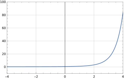
Figure 1: A plot of $\left|f^{\mbox{\tiny airy}}(t)\right|$, where $f^{\mbox{\tiny airy}}(t)=\mbox{Ai}(t)+i\mbox{Bi}(t)$. In contrast to $f^{\mbox{\tiny airy}}$, the absolute values of most solutions of Airy’s differential equation are oscillatory on the negative real axis.

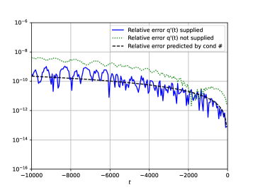
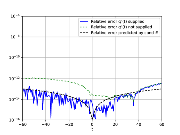
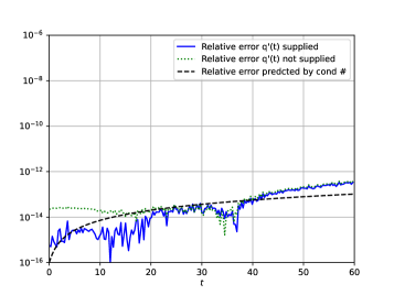
Figure 6: The results of the experiments discussed in Subsection 5.1, which concerned the Airy functions. The plots in the first row compare the relative errors incurred when evaluating $f^{\mbox{\tiny airy}}(t)=\mbox{Ai}(t)+i\mbox{Bi}(t)$ using the phase functions $\alpha^{\mbox{\tiny airy}}$ and $\widetilde{\alpha}^{\mbox{\tiny airy}}$ with the relative error predicted by its condition number of evaluation. The plot in the upper left is given over the interval $(-10000,0)$, and that on the upper right is given over the interval $(-60,60)$. The plot on the lower left gives the absolute error in the calculated values of $\mbox{Ai}(t)$ in the interval $(-60,0)$ as a function of $t$, while that on the lower right gives the relative error in the calculated value of $\mbox{Ai}(t)$ in the interval $(0,60)$ as a function of $t$ and compares it with the relative error predicted by the condition number of evaluation of $\mbox{Ai}(t)$.

In our first experiment, we used each of the two phase functions to evaluate $f^{\mbox{\tiny airy}}$ at $200$ equispaced points on the interval $(-10,000,0)$, where the Airy functions are oscillatory. The plot on the left-hand side of the top row of Figure 6 gives the results. There, the relative errors in the values of $f^{\mbox{\tiny airy}}$ calculated using each of the two phase functions are plotted, as are the relative errors predicted by the condition number of evaluation of this function.

In our next experiment, we used the each of the two phase functions to evaluate $f^{\mbox{\tiny airy}}$ at $200$ equispaced points on the interval $(-60,60)$. The plot on the right-hand side of the top row of Figure 6 compares the relative errors which were incurred when doing so with those predicted by the condition number of evaluation of $f^{\mbox{\tiny airy}}$ .

In a third experiment related to the Airy functions, we used the phase function for (88) to evaluate Ai at $200$ equispaced points in the interval $(-60,0)$ using each of the two phase functions for (88). Since Ai is oscillatory on this interval and has many zeros there, it is not sensible to measure the relative errors in these calculations. Instead, we measured the absolute errors incurred when Ai was evaluated using $\alpha^{\mbox{\tiny airy}}$ and $\widetilde{\alpha}^{\mbox{\tiny airy}}$. The plot on the left-hand side of the second row of Figure 6 gives the results.

In a last experiment concerning the Airy functions, we used the two phase functions for (88) to evaluate Ai at $200$ equispaced points on the interval $(0,60)$. The plot on the right-hand side of the second row of Figure 6 gives the results. There, the relative errors in the values of Ai calculated using each of the two phase functions are plotted, as are the relative errors predicted by the condition number of evaluation of Ai.

5.2 Bessel functions

In this set of experiments, we constructed phase functions for the normal form

$$y^{\prime\prime}(t)+\left(1+\frac{\frac{1}{4}-\nu^{2}}{t^{2}}\right)y(t)=0,\ \ 0<t<\infty,$$ (90)

of Bessel’s differential equation. When $\nu>\frac{1}{2}$,

$$c=\frac{1}{2}\sqrt{4\nu-1}$$ (91)

is a turning point of order $1$ for (90). The coefficient in (90) is negative on the interval $(0,c)$ and positive on $(c,\infty)$. Standard solutions include the Bessel functions of the first and second kinds $J_{\nu}$ and $Y_{\nu}$ (definitions of which were given in Subsection 3.1).

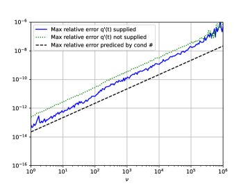
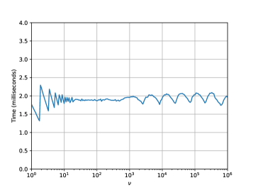
Figure 7: The results of the first experiment of Section 5.2, which concerned the Bessel functions. The plot on the left gives the maximum relative errors which were observed in the course of evaluating the Bessel function $f_{\nu}^{\mbox{\tiny bes}}=J_{\nu}(t)+iY_{\nu}(t)$ at $5,000$ equispaced on the interval $(0,100\nu)$ using the phase functions $\alpha^{\mbox{\tiny bes}}_{\nu}$ and $\widetilde{\alpha}^{\mbox{\tiny bes}}_{\nu}$, as well as the maximum relative error predicted by the condition number of evaluation of $f_{\nu}^{\mbox{\tiny bes}}$, as functions of $\nu$. The plot on the right gives the time (in milliseconds) which was required to construct the phase function $\alpha^{\mbox{\tiny bes}}_{\nu}$ as a function of $\nu$.

In the first experiment, we sampled $m=200$ equispaced points $x_{1},x_{2},\ldots,x_{m}$ in the interval $[0,6]$ and constructed phase functions $\alpha_{\nu}^{\mbox{\tiny bes}}$ and $\widetilde{\alpha}_{\nu}^{\mbox{\tiny bes}}$ for each $\nu=10^{x_{1}},10^{x_{2}},\ldots,10^{x_{m}}$. In the case of $\alpha^{\mbox{\tiny bes}}_{\nu}$, the derivative of the coefficient was supplied as input and in the case of $\widetilde{\alpha}^{\mbox{\tiny bes}}_{\nu}$, the derivative was calculated via spectral differentiation. We then used each of these phase functions to evaluate the function $f_{\nu}^{\mbox{\tiny bes}}(t)=J_{\nu}(t)+iY_{\nu}(t)$ at $5,000$ equispaced points on the interval $(0,100\nu)$. We considered the function $f_{\nu}^{\mbox{\tiny bes}}$ rather than the Bessel functions individually because its absolute value is nonoscillatory; indeed, it was shown in Section 3.1 that $\left|f_{\nu}^{\mbox{\tiny bes}}\right|^{2}$ is completely monotone on $(0,\infty)$. The plot on the left-hand side of Figure 7 gives the maximum observed relative errors as functions of $\nu$, as well as the maximum relative error predicted by the condition number of evaluation of $f^{\mbox{\tiny bes}}_{\nu}$. The plot on the right-hand side of Figure 7 gives the time require to construct the phase function $\alpha_{\nu}^{\mbox{\tiny bes}}$ as a function of $\nu$.

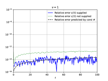
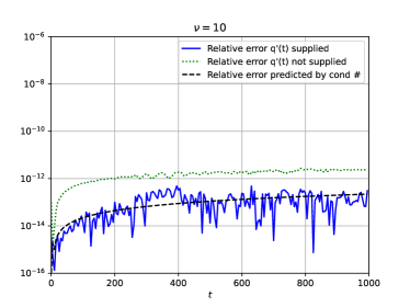
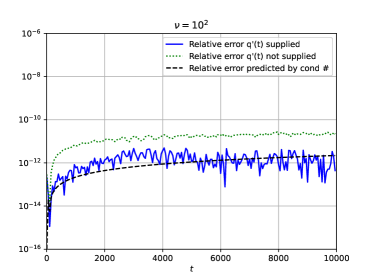
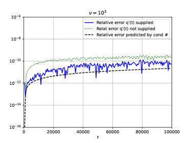
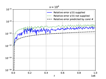
Figure 8: The results of the second set of experiments discussed in Subsection 5.2, which concerned the Bessel functions. Each plot gives the relative errors in the values of $f_{\nu}^{\mbox{\tiny bes}}(t)=J_{\nu}(t)+iY_{\nu}(t)$ calculated using the phase functions $\alpha_{\nu}^{\mbox{\tiny bes}}$ and $\widetilde{\alpha}_{\nu}^{\mbox{\tiny bes}}$ for a particular fixed value of $\nu$ as a function of $t$, and compares them with the relative error predicted by the condition number of evaluation of $f_{\nu}^{\mbox{\tiny bes}}$.

In a second set of experiments, for each $\nu=1,10,10^{2},\ldots,10^{5}$, we measured the relative errors incurred when the phase functions $\alpha_{\nu}^{\mbox{\tiny bes}}$ and $\widetilde{\alpha}_{\nu}^{\mbox{\tiny bes}}$ were used to evaluate $f^{\mbox{\tiny bes}}_{\nu}(t)$ at $200$ equispaced spaced points in the interval $(0,100\nu)$. Figure 8 gives the results. Each plot there corresponds to a different value of $\nu$, and gives the relative errors incurred when the phase functions were used to evaluate $f^{\mbox{\tiny bes}}_{\nu}(t)$, as well as the relative error predicted by its condition number of evaluation, as functions of $t$.

5.3 Associated Legendre functions

The experiments described in this subsection concern the associated Legendre differential equation

$$(1-t^{2})y^{\prime\prime}(t)-ty(t)+\left(\nu(\nu+1)-\frac{\mu^{2}}{1-t^{2}}\right)y(t)=0,\ \ -1<t<1.$$ (92)

Standard solutions of (92) defined on the interval $(-1,1)$ include the Ferrer’s functions of the first and second kinds $P_{\nu}^{\mu}$ and $Q_{\nu}^{\mu}$ (see, for instance, [4] or [16] for definitions). The Ferrer’s functions of negative orders are generally better behaved than those of positive orders — for instance, when $\mu\geq 0$ is not an integer, $P_{\nu}^{\mu}(t)$ is singular at $t=1$ whereas $P_{\nu}^{-\mu}(t)$ is not — and they coincide in the important case of integer values of $\nu$ and $\mu$. When $\nu\geq\left|\mu\right|$ (this is a standard requirement), the normalizations

$$\widetilde{P}_{\nu}^{\mu}(t) =\sqrt{\left(\nu+\frac{1}{2}\right)\frac{\Gamma\left(\nu+\mu+1\right)}{\Gamma\left(\nu-\mu+1\right)}}\ P_{\nu}^{\mu}(t),\ \ \mbox{and}$$ (93)

$$\widetilde{Q}_{\nu}^{\mu}(t) =\sqrt{\left(\nu+\frac{1}{2}\right)\frac{\Gamma\left(\nu+\mu+1\right)}{\Gamma\left(\nu-\mu+1\right)}}\ Q_{\nu}^{\mu}(t)$$

are well-defined, and we prefer them to the standard Ferrer’s functions because the latter can take on extremely large and extremely small values, even when $\nu$ and $\mu$ are of modest sizes. We note that the $L^{2}(-1,1)$ norm of $\widetilde{P}_{\nu}^{-\mu}$ is $1$ when both $\nu$ and $\mu$ are integers.

We claim that the phase function generated by the pair

$$\widetilde{P}_{\nu}^{-\mu}(t),\ \ \frac{2}{\pi}\widetilde{Q}_{\nu}^{-\mu}(t)$$ (94)

is nonoscillatory in a rather strong sense. To see this, we first observe that

$$\widetilde{P}_{\nu}^{-\mu}(t)+i\frac{2}{\pi}\widetilde{Q}_{\nu}^{-\mu}(t)= \frac{2}{\pi}\sqrt{\frac{\nu+\frac{1}{2}}{\Gamma\left(\nu+\mu+1\right)\Gamma\left(\nu-\mu+1\right)}}\exp\left(i\frac{\pi}{2}\left(\mu-\nu\right)\right)\left(\frac{1}{1-t^{2}}\right)^{\frac{\nu+1}{2}}$$ (95)

$$\int_{0}^{\infty}\exp\left(ix\frac{t}{\sqrt{1-t^{2}}}\right)K_{\mu}(x)x^{\nu}\ dx,$$

where $K_{\nu}$ is the modified Bessel function of the third kind of order $\mu$. This formula appears in a slightly different form in Section 7.8 of [3], and it can be verified quite easily — for instance, by showing that the expression appearing on the right-hand side satisfies Appell’s differential equation and then verifying that the functions appearing on the left- and right-hand sides and their first two derivatives agree at $0$. Next, we make the change of variables

$$t=\frac{p}{\sqrt{1+p^{2}}}$$ (96)

to obtain

$$\widetilde{P}_{\nu}^{-\mu}\left(\frac{p}{\sqrt{1+p^{2}}}\right)+i\frac{2}{\pi}\widetilde{Q}_{\nu}^{-\mu}\left(\frac{p}{\sqrt{1+p^{2}}}\right)= \frac{2}{\pi}\sqrt{\frac{\nu+\frac{1}{2}}{\Gamma\left(\nu+\mu+1\right)\Gamma\left(\nu-\mu+1\right)}}\exp\left(i\frac{\pi}{2}\left(\mu-\nu\right)\right)$$ (97)

$$\left(1+p^{2}\right)^{\frac{\nu+1}{2}}\int_{0}^{\infty}\exp\left(itp\right)K_{\mu}(t)t^{\nu}\ dt.$$

We now observe that

$$\left(\widetilde{P}_{\nu}^{-\mu}\left(\frac{p}{\sqrt{1+p^{2}}}\right)\right)^{2}+\left(\frac{2}{\pi}\widetilde{Q}_{\nu}^{-\mu}\left(\frac{p}{\sqrt{1+p^{2}}}\right)\right)^{2}$$ (98)

$$\ \ =\frac{4}{\pi^{2}}\ \frac{(1+p^{2})^{\nu+1}\left(\nu+\frac{1}{2}\right)}{\Gamma\left(\nu-\mu+1\right)\Gamma\left(\nu+\mu+1\right)}\int_{-\infty}^{\infty}\exp(itp)G(t)\ dt,$$

where

$$G(t)=\int_{\max(0,-t)}^{\infty}K_{\mu}(t+s)(t+s)^{\nu}K_{\mu}(s)s^{\nu}\ ds.$$ (99)

Since

$$K_{\mu}(z)\sim\sqrt{\frac{\pi}{2z}}\exp(-z)\ \ \mbox{as}\ \ z\to\infty,$$ (100)

the function $K_{\mu}(t)t^{\nu}$ behaves similarly to a bump function centered at the point $\nu-1/2$ when $\nu$ is of large magnitude. It follows that the function $G$ defined in (99) resembles a bump function centered around the point $0$, again assuming $\nu$ is of large magnitude. In particular, the function (98) is nonoscillatory in the sense that its Fourier transform resembles a rapidly decaying bump function centered at $0$. Figure 2 contains plots of the functions $1/\Gamma(\nu)K_{\mu}(t)t^{\nu}$ and $1/\Gamma(\nu)^{2}G(t)$ when $\nu=100$ and $\mu=20$. The scaling by the reciprocal of $\Gamma(\nu)$ was introduced because the magnitudes of these functions are quite large otherwise.

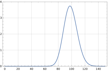
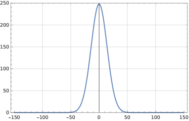
Figure 2: On the left is a plot of the function $1/\Gamma(\nu)K_{\mu}(t)t^{\nu}$ when $\nu=100$ and $\mu=20$. On the right is a plot of $1/\Gamma(\nu)^{2}G(t)$, where $G$ is the function defined in (99), when $\nu=100$ and $\mu=20$.

When performing numerical computations involving the associated Legendre functions, it is convenient to introduce a change of variables which eliminates the singular points of the equation (92) at $\pm 1$. If $y$ solves (92), then

$$z(w)=y(\tanh(w))$$ (101)

satisfies

$$z^{\prime\prime}(w)+\left(\nu(\nu+1)\sech^{2}(w)-\mu^{2}\right)z(w)=0,\ \ -\infty<w<\infty.$$ (102)

We use $\alpha_{\nu,\mu}^{\mbox{\tiny alf}}$ to denote the phase function for (102) constructed via the algorithm of this paper with values of the derivative of the coefficient supplied, and $\widetilde{\alpha}_{\nu,\mu}^{\mbox{\tiny alf}}$ to denote the phase function for (102) constructed via the algorithm of this paper with derivatives of the coefficient calculated using spectral differentiation.

In each experiment of this subsection, we first fixed a value of $\mu$ and sampled $m=200$ equispaced points $x_{1},\ldots,x_{m}$ in the interval $[0,6]$. Then, for each $\lambda=10^{x_{1}},10^{x_{2}},\ldots,10^{x_{m}}$, we constructed phase functions $\alpha_{|\mu|+\lambda,\mu}^{\mbox{\tiny alf}}$ and $\widetilde{\alpha}_{|\mu|+\lambda,\mu}^{\mbox{\tiny alf}}$ using the algorithm of this paper. In the case of $\alpha_{|\mu|+\lambda,\mu}^{\mbox{\tiny alf}}$, the values of the derivatives of the coefficient were supplied to the algorithm, while spectral differentiation was used to evaluate $q^{\prime}(t)$ in the case of $\widetilde{\alpha}_{|\mu|+\lambda,\mu}^{\mbox{\tiny alf}}$. To be clear, the degree $\nu$ of the associated Legendre function was taken to be $\nu=|\mu|+\lambda$ (it is necessary for $\nu\geq|\mu|$). The phase functions were given on intervals of the form $[0,b]$ with $b$ chosen by our algorithm so that the value of the derivative of $\alpha_{|\mu|+\lambda,\mu}^{\mbox{\tiny alf}}$ there was close to the smallest representable IEEE double precision number. For each chosen value of $\lambda$, we used both of the corresponding phase functions to evaluate

$$f_{|\mu|+\lambda,\mu}^{\mbox{\tiny alf}}(w)=\widetilde{P}_{|\mu|+\lambda}^{\mu}(\tanh(w))+\frac{2}{\pi}i\widetilde{Q}_{|\mu|+\lambda}^{\mu}(\tanh(w))$$ (103)

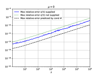
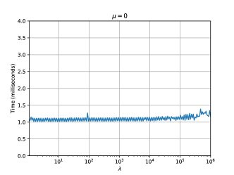
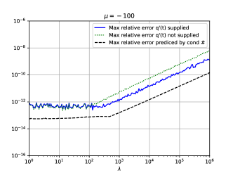
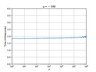
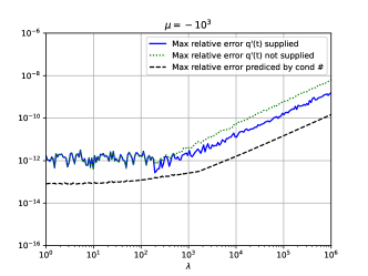
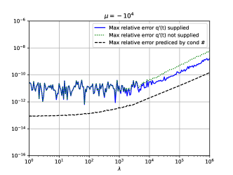
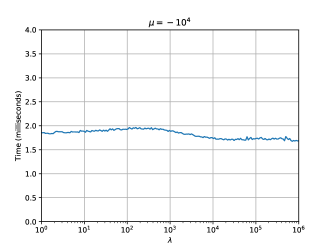
Figure 9: The results of the experiments discussed in Subsection 5.3, which concerned the associated Legendre functions. The left-hand side of each row contains a plot giving the maximum relative errors observed while calculating the values of $f^{\mbox{\tiny alf}}_{\lambda,\mu}(w)=\widetilde{P}_{|\mu|+\lambda}^{\mu}(\tanh(w))+i\frac{2}{\pi}\widetilde{Q}_{|\mu|+\lambda}^{\mu}(\tanh(w))$ at $5,000$ points using each of the phase functions $\alpha_{|\mu|+\lambda,\mu}^{\mbox{\tiny alf}}$ and $\widetilde{\alpha}_{|\mu|+\lambda,\mu}^{\mbox{\tiny alf}}$, as well as the the maximum relative error predicted by the condition number of evaluation of $f^{\mbox{\tiny alf}}_{|\mu|+\lambda,\mu}(w)$, as functions of $\lambda$ for a fixed value of $\mu$. The right-hand side of each row contains a plot giving the time (in milliseconds) required to construct the phase function representing $f^{\mbox{\tiny alf}}_{|\mu|+\lambda,\mu}(w)$ as a function of $\lambda$.

at $5,000$ equispaced points on the interval $[0,b]$. Figure 9 reports the results. Each row in that figure corresponds to one experiment. The plot on the left-hand side gives the maximum relative errors observed while evaluating (103) using each of the phase functions $\alpha_{|\mu|+\lambda,\mu}^{\mbox{\tiny alf}}$ and $\widetilde{\alpha}_{|\mu|+\lambda,\mu}^{\mbox{\tiny alf}}$, as well as the maximum relative error predicted by the condition number of evaluation of $f_{|\mu|+\lambda,\mu}^{\mbox{\tiny alf}}$, as functions of $\lambda$. The plot on the right gives the time (in milliseconds) required to construct $\alpha_{|\mu|+\lambda,\mu}^{\mbox{\tiny alf}}$ as a function of $\lambda$.

Remark 1.

Formula (97) implies that, after a suitable change of variables, the function $\widetilde{P}_{\nu}^{-\mu}(t)+i\frac{2}{\pi}\widetilde{Q}_{\nu}^{-\mu}(t)$ is an element of one of the Hardy spaces of functions analytic in the upper half of the complex plane (see, for instance, [13] for a careful discussion of such spaces). Likewise, Formula (49) shows that $J_{\nu}(z)+iY_{\nu}(z)$ is an element of one of these Hardy spaces as well. It is not a coincidence that these two functions give rise to slowly varying phase functions. A relatively straightforward generalization of the discussion in Subsection 5.3 shows that when a second order differential equation with slowly varying coefficients admits a solution in one of the classical Hardy spaces of functions analytic in the upper half of the complex plane (perhaps after a change of variables), it will have a slowly varying phase function. This argument applies to Bessel’s differential equation, the spheroidal wave equation, and many other second order linear ordinary differential equations.

5.4 Equations with turning points of higher orders

The experiments described in this subsection concerned the differential equation

$$y^{\prime\prime}(t)+t^{k}y(t)=0,\ \ -10<t<10,$$ (104)

with $k$ a positive integer greater than $1$. In the event that $k$ is even, the functions $u_{k}^{\mbox{\tiny even}}$ and $v_{k}^{\mbox{\tiny even}}$ defined in (53) and (54) form a basis in the space of solutions of (104). It can be verified using a argument similar to that of Subsection 3.2 that

$$u_{k}^{\mbox{\tiny odd}}(t)=\begin{cases}\sqrt{\frac{\pi t}{2+k}}J_{\frac{1}{2k}}\left(t^{1+\frac{k}{2}}{1+\frac{k}{2}}\right)&\mbox{if}\ \ t>0\\ \sqrt{-\frac{-\pi t}{2+k}}I_{\frac{1}{2k}}\left((-t)^{1+\frac{k}{2}}{1+\frac{k}{2}}\right)&\mbox{if}\ \ t<0\\ \end{cases}$$ (105)

and

$$v_{k}^{\mbox{\tiny odd}}(t)=\begin{cases}\sqrt{\frac{\pi t}{2+k}}Y_{\frac{1}{2k}}\left(\frac{t^{1+\frac{k}{2}}}{1+\frac{k}{2}}\right)&\mbox{if}\ \ t>0\\ d_{1}\sqrt{-\frac{-\pi t}{2+k}}I_{\frac{1}{2k}}\left(\frac{(-t)^{1+\frac{k}{2}}}{1+\frac{k}{2}}\right)+d_{2}\sqrt{-\frac{-\pi t}{2+k}}I_{-\frac{1}{2k}}\left(\frac{(-t)^{1+\frac{k}{2}}}{1+\frac{k}{2}}\right)&\mbox{if}\ \ t<0,\\ \end{cases}$$ (106)

where $I_{\nu}$ is the modified Bessel function of the first kind,

$$d_{1}=\sqrt{\pi}\cos\left(\frac{\pi(1+k)}{2+k}\right)\csc\left(\frac{\pi}{2+k}\right)\ \ \mbox{and}\ \ d_{2}=\frac{\sqrt{\pi}\csc\left(\frac{\pi}{2+k}\right)}{\sqrt{2+k}},$$ (107)

form a basis in the space of solutions of (104) when $k$ is odd.

In each experiment, a value of $k$ was fixed and the algorithm of this paper was applied twice to evaluate

$$f_{k}^{\mbox{\tiny high}}(t)=\begin{cases}u_{k}^{\mbox{\tiny even}}(t)+iv_{k}^{\mbox{\tiny even}}(t)&\mbox{if k is even}\\ u_{k}^{\mbox{\tiny odd}}(t)+iv_{k}^{\mbox{\tiny odd}}(t)&\mbox{if k is odd}\end{cases}$$ (108)

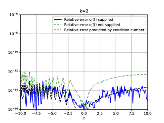
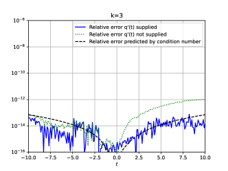
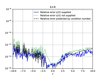
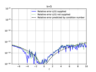
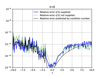
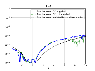
Figure 10: The results of the experiments discussed in Subsection 5.4, which concerned an equation with a turning point of order $k$. Each plot corresponds to one value of $k$ and gives the relative errors incurred when the function $f_{k}^{\mbox{\tiny high}}$ defined via (108) was evaluated at $200$ equispaced points using the algorithm of this paper with the derivatives of the coefficients supplied, the relative errors incurred when $f_{k}^{\mbox{\tiny high}}$ was evaluated at $200$ equispaced points using the algorithm of this paper with the derivatives of the coefficients calculated via spectral differentiation, and the relative errors predicted by the condition number of evaluation of $f_{k}^{\mbox{\tiny high}}$ .

at $200$ equispaced points. The first time the algorithm was executed, the values of the derivative of the coefficient in (104) were supplied, and during the second application of the algorithm, the derivative of the coefficient was evaluated using spectral differentiation. The results appear in Figure 10. Each plot there corresponds to one value of $k$ and gives the relative errors in the calculated values of $f_{k}^{\mbox{\tiny high}}(t)$ incurred by each variant of the algorithm, as well as the relative errors predicted by the condition number of evaluation of $f_{k}^{\mbox{\tiny high}}$.

5.5 An equation whose coefficient has two bumps

In this experiment, we considered the boundary value problem

$$\left\{\begin{aligned} y^{\prime\prime}(t)+\nu^{2}q(t)y(t)&=0,\ \ -10<t<10,\\ y(0)&=0\\ y^{\prime}(10)&=1,\end{aligned}\right.$$ (109)

where

$$q(t)=\exp\left(-(t-5)^{2}\right)+\exp\left(-(t+5)^{2}\right)+\frac{\sin\left(\frac{t}{2}\right)^{2}}{1+t^{2}}.$$ (110)

The function $q$, a graph of which appears on the left-hand side of Figure 3, has a single zero at the point $t=0$. A plot of the solution of (109) when $\nu=50$ appears on the right-hand side of Figure 3.

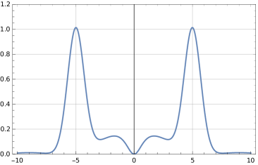
Figure 3: A graph of the coefficient $q(t)$ in the ordinary differential equation considered in Subsection 5.5 appears on the left. It has a single zero at the point $t=0$. On the right is a graph of the solution of the problem (109) when $\nu=50$. In the experiments of the paper, we consider values of $\nu$ as large as $10^{6}$ — we plot the solution in the case of a relatively small value of $\nu$ to give the reader an indication of the behavior of the solutions and not as an illustration of the performance of our algorithm.

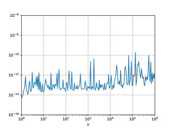
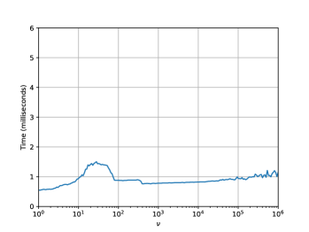
Figure 11: The results of the experiments discussed in Subsection 5.5, which concerned an equation whose coefficient has two bumps. On the left we give the maximum absolute difference between the solution obtained with the phase method and that obtained using a standard solver running in extended precision as a function of $\nu$. On the right is a plot giving the time taken to solve the problem (109) using the phase method as a function of $\nu$.

In this experiment, we sampled $m=200$ points $x_{1},\ldots,x_{m}$ in the interval $[0,6]$. Then, for each $\nu=10^{x_{1}},\ 10^{x_{2}},\ldots,10^{x_{m}},$ we solved (109) using the algorithm of this paper with the values of $q^{\prime}$ specified. We also solved (109) by running the standard solver described in Subsection 4.1 using extended precision arithmetic. We then calculated the absolute difference in the obtained solutions at $5,000$ equispaced points in the interval $(-10,10)$. The plot on the left-hand side of Figure 11 gives the largest observed maximum absolute difference as a function of $\nu$. The plot on the right-hand side gives the times required to solve (109) using the phase method as a function of $\nu$.

5.6 An equation with three turning points

In this experiment, we considered the problem

$$\left\{\begin{aligned} y^{\prime\prime}(t)+\nu^{2}q(t)y(t)&=0,\ \ -10<t<10,\\ y(0)&=1\\ y^{\prime}(0)&=0,\end{aligned}\right.$$ (111)

where

$$q(t)=\exp\left(-(t+5)^{2}\right)-(t-5)\exp\left(-(t-5)^{2}\right)-6\exp(-25).$$ (112)

The coefficient $q$ has three zeros on the interval $(-10,10)$:

$$c_{1} \approx-9.817493179110059,$$ (113)

$$c_{2} =0\ \ \mbox{and}$$

$$c_{3} \approx 4.999999999916672.$$

A graph of the function $q$ appears in Figure 4, as does a plot of the solution of (111) over the interval $(-10,5.5)$ when $\nu=50$. We truncated the plot of the solution because its magnitude grows quickly in the interval $(c_{3},10)$.

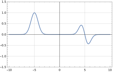
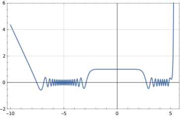
Figure 4: A graph of the coefficient $q(t)$ in the ordinary differential equation considered in Subsection 5.6 appears on the left. On the right is a graph of the solution of the problem (111) over the interval $(-10,5.5)$ when $\nu=50$. The plot was truncated because the magnitude of the solution grows quickly in the interval $(c_{3},10)$. In the experiments of the paper, we consider values of $\nu$ as large as $10^{5}$ — we plot the solution in the case of a relatively small value of $\nu$ to give the reader an indication of the behavior of the solutions and not as an illustration of the performance of our algorithm.

In this experiment, we first sampled $m=200$ points $x_{1},\ldots,x_{m}$ in the interval $[0,5]$. Then, for each $\nu=10^{x_{1}},\ 10^{x_{2}},\ldots,10^{x_{m}}$, we solved (111) using a phase function method. More explicitly, we constructed two phase functions, one defined on the interval $(-10,0)$ and the second defined on the interval $(0,10)$. The windowing algorithm was used on an interval around the point $-5$ to determine the correct initial values for the phase function on $(-10,0)$ and the windowing algorithm was applied on an interval around the point $3$ to determine the initial values for the phase function given on $(0,10)$. The values of $q^{\prime}$ were specified. We next solved the problem (111) using the standard solver described in Subsection 4.1 running in extended precision arithmetic. Then, we evaluated the solution $y_{1}$ obtained with the phase method and the solution $y_{2}$ constructed by the standard solver at $r=5,000$ equispaced points $z_{1},z_{2},\ldots,z_{r}$ on the interval $(-10,10)$ and measured the quantity

$$\xi_{\nu}=\max_{1\leq j\leq 5000}\frac{\left|y_{1}(z_{j})-y_{2}(z_{j})\right|}{1+\left|y_{2}(z_{j})\right|}.$$ (114)

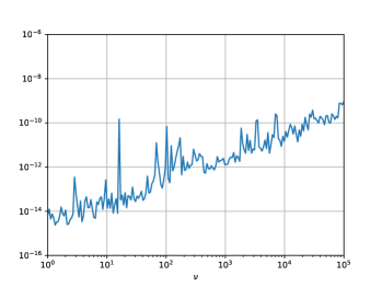
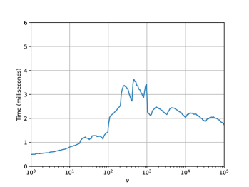
Figure 12: The results of the experiments discussed in Subsection 5.6, which concerned an equation whose coefficient has three turning points. On the left is a plot of a measure of the maximum difference between the solution obtained via a phase function method and that obtained using a standard solver running in extended precision as a function of $\nu$. On the right is a plot giving the time taken to solve the problem (109) using the phase method as a function of $\nu$.

Neither the absolute nor relative differences between the two solutions were appropriate for this problem because the solution of (111) oscillates on part of the interval and it is of large magnitude in another region. Figure 12 gives the results. On the left-hand side is a plot of $\xi_{\nu}$ as a function of $\nu$, while the plot on the right-hand side gives the times required to solve (111) via the phase method as a function of $\nu$.

5.7 An equation with many turning points

In this experiment, we considered the problem

$$\left\{\begin{aligned} y^{\prime\prime}(t)+\nu^{2}q(t)y(t)&=0,\ \ -11<t<11,\\ y(0)&=1\\ y^{\prime}(0)&=1,\end{aligned}\right.$$ (115)

where

$$q(t)=1+\cos\left(\pi t\right).$$ (116)

The coefficient $q$ has $12$ zeroes in the interval $(-11,11)$, at the points

$$-11,-9,-7,\ldots,-1,1,\ldots,7,9,11.$$

A graph of the function $q$ appears in Figure 5, as does a plot solution of (115) when $\nu=20$.

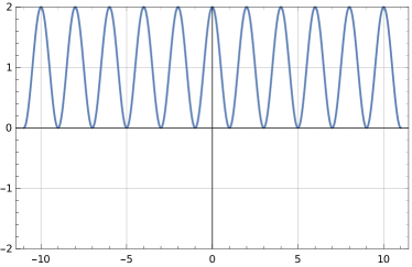
Figure 5: A graph of the coefficient $q(t)$ appearing in the ordinary differential equation considered in Subsection 5.7 appears on the left. On the right is a graph of the solution of the problem (115) when $\nu=20$. In the experiments of the paper, we consider values of $\nu$ as large as $10^{5}$ — we plot the solution in the case of a relatively small value of $\nu$ to give the reader an indication of the behavior of the solutions and not as an illustration of the performance of our algorithm.

We sampled $m=200$ points $x_{1},\ldots,x_{m}$ in the interval $[0,5]$. Then, for each $\nu=10^{x_{1}},\ 10^{x_{2}},\ldots,10^{x_{m}}$, we solved (111) using a phase function method and with the standard solver described in Subsection 4.1 running in extended precision arithmetic. To solve (115) using phase functions, we constructed eleven phase functions, one on each of the intervals

$$\left(-1+2k,1+2k\right),\ \ k=-5,-4,\ldots,-1,0,1,\ldots,4,5.$$ (117)

The values of $q^{\prime}$ were specified.

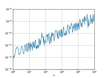
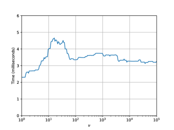
Figure 13: The results of the experiments discussed in Subsection 5.7, which concerned an equation whose coefficient has $12$ turning points. On the left is a plot of the maximum absolute difference between the solution obtained with the phase method and that obtained via a standard solver running in extended precision as a function of $\nu$. On the right is a plot giving the time taken to solve the problem (109) using the phase method as a function of $\nu$.

Figure 13 gives the results. The plot on the left-hand side gives the maximum absolute difference in the solutions obtained by the two solvers observed while evaluating them at $5,000$ equispaced points in the interval $(-11,11)$ as a function of $\nu$. The plot on the right-hand side gives the times required to solve (115) using the phase method as a function of $\nu$.

6 Conclusions

We have described a variant of the algorithm of [7] for the numerical solution of a large class of second order linear ordinary differential equations, including many with turning points. Unlike standard solvers, its running time is largely independent of the magnitude of the coefficients appearing in the equation, and, unlike asymptotic methods, it consistently achieves accuracy on par with that indicated by the condition number of the problem.

One of the key observations of [7] is that it is often preferable to calculate phase functions numerically by simply solving the Riccati equation rather than constructing asymptotic approximations of them à la WKB methods. A principal observation of this paper is that, unlike standard asymptotic approximations of solutions of the Riccati equation which become singular near turning points, the phase functions themselves are perfectly well-behaved near turning points, and this can be exploited to avoid using different mechanisms to represent solutions in different regimes. It appears from numerical experiments that, in the vicinity of turning points, the cost of representing phase functions via Chebyshev expansions and the like is comparable to that of representing the solutions themselves. And, perhaps surprisingly, solutions can be represented to high relative accuracy deep into the nonoscillatory regime via phase functions.

We have also presented experiments showing that the algorithm of this paper can be used to evaluate many families of special functions in time independent of their parameters. It should be noted, however, that using precomputed piecewise polynomial expansions of phase functions for the second order linear ordinary differential equations satisfied by various families of special functions is much faster. Because these phase functions are slowly varying, the expansions are surprisingly compact. We refer the interested reader to [6], where such an approach is used to evaluate the associated Legendre functions.

Phase functions methods are highly useful for performing several other computations involving special functions. For instance, they can be used to calculate their zeros and various generalized Gaussian quadrature rules [5], and the author will soon report on a method for rapidly applying special function transforms using phase functions.

In a future work, the author will describe an extension of the algorithm of this paper which combines standard solvers for second order differential equations with phase function methods. The algorithm will operate by subdividing the solution domain into intervals and constructing a local basis of solutions on each interval. When the coefficients are of large magnitude, the local basis functions will be represented via phase functions, and the basis functions will be represented directly, via piecewise Chebyshev expansions, on intervals in which the coefficients are of small magnitude. One of the principal advantages of such an approach is that the solution interval can be subdivided in a more or less arbitrary fashion and each computation can be performed locally, thus allowing for large-scale parallelization.

7 Acknowledgments

The author would like to thank Alex Barnett and Fruzsina Agocs of the Flatiron Institute and Kirill Serkh of the University of Toronto for many thoughtful discussions and suggestions. The author was supported in part by NSERC Discovery grant RGPIN-2021-02613.

References

- [1] Appell, P. Sur la transformation des équations différentielles linéaires. Comptes Rendus 91 (1880), 211–214.
- [2] Ascher, U. M., and Petzold, L. R. Computer Methods for Ordinary Differential Equations and Differential-Algebraic Equations. Society for Industrial and Applied Mathematics, USA, 1998.
- [3] Bateman, H., and Erdélyi, A. Higher Transcendental Functions, vol. II. McGraw-Hill, 1953.
- [4] Bateman, H., and Erdélyi, A. Higher Transcendental Functions, vol. I. McGraw-Hill, 1953.
- [5] Bremer, J. On the numerical calculation of the roots of special functions satisfying second order ordinary differential equations. SIAM Journal on Scientific Computing 39 (2017), A55–A82.
- [6] Bremer, J. An algorithm for the numerical evaluation of the associated Legendre functions that runs in time independent of degree and order. Journal of Computational Physics 360 (2018), 15–28.
- [7] Bremer, J. On the numerical solution of second order differential equations in the high-frequency regime. Applied and Computational Harmonic Analysis 44 (2018), 312–349.
- [8] Bremer, J. A quasilinear complexity algorithm for the numerical simulation of scattering from a two-dimensional radilly symmetric potential. Journal of Computation Physics (2020).
- [9] Bremer, J., and Rokhlin, V. Improved estimates for nonoscillatory phase functions. Discrete and Continuous Dynamical Systems, Series A 36 (2016), 4101–4131.
- [10] Greengard, L. Spectral integration and two-point boundary value problems. SIAM Journal of Numerical Analysis 28 (1991), 1071–1080.
- [11] Hartman, P. On differential equations, Volterra equations and the function . American Journal of Mathemtics 95 (1973), 553–593.
- [12] Higham, N. J. Accuracy and Stability of Numerical Algorithms, second ed. SIAM, 2002.
- [13] Koosis, P. An introduction to spaces, second ed. Cambridge University Press, 2008.
- [14] Kummer, E. De generali quadam aequatione differentiali tertti ordinis. Progr. Evang. Köngil. Stadtgymnasium Liegnitz (1834).
- [15] Miller, P. D. Applied Asymptotic Analysis. American Mathematical Society, 2006.
- [16] Olver, F. W. Asymptotics and Special Functions. A.K. Peters, 1997.
- [17] Spigler, R. Asymptotic-numerical approximations for highly oscillatory second-order differential equations by the phase function method. Journal of Mathematical Analysis and Applications 463 (2018), 318–344.
- [18] Spigler, R., and Vianello, M. A numerical method for evaluating the zeros of solutions of second-order linear differential equations. Mathematics of Computation 55 (1990), 591–612.
- [19] Spigler, R., and Vianello, M. The phase function method to solve second-order asymptotically polynomial differential equations. Numerische Mathematik 121 (2012), 565–586.
- [20] Widder, D. The Laplace Transform. Princeton University Press, 1946.