Task Graph Formulation

 

We are considering directed, acyclic graphs where each node represents a task and edges between nodes represent a relationship (or influence) between the rewards of the two tasks. Most often, this relationship is some form of precedence constraint: if node A is connected to node B by a directed edge, then the reward from task B depends heavily on the proper completion of task A.

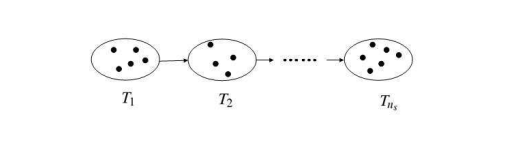
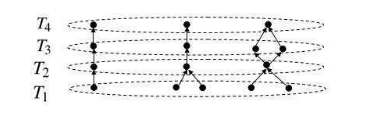
Figure 1: Task graph with set precedence constraints as presented in [Luo2011]. All tasks in each node have the same completion time.

We begin with a homogeneous group of $n$ robots. The robots are represented as units of flow on the graph. To allocate tasks to the robots we solve a min-cost flow problem: if a set of robots is flowing through node A, then all these robots are assigned to node A. The tasks are performed with cost $\mathbf{c}_{i},i\in\{1..n\}$, where $c_{i}$ is a random variable (assume Gaussian) parameterized by a mean $\mu_{i}$ and variance $\sigma_{i}^{2}$. This mean and variance depend upon two factors: (1) the coalition assigned to the task, i.e. the set of robots flowing through the task node, and (2) the In [Mitchell2015], the authors use a similar mechanism to represent an uncertain estimate of task cost, and to update this estimate as robots execute tasks. In their setting, the task cost represented the amount of energy it consumed, and its value was updated via noisy measurements of the energy reserve level.

The task costs at each node are projected onto the incoming edges to the node, making them edge weights. (could this also be outgoing edges? does it make a difference?)

Branches in the graph represent alternate sets of tasks that can be completed to fulfill the precedence constraints of future nodes.

Robots move through the graph, updating their estimates of the task cost probability density functions as they get new observations (i.e. observe success/failure while trying to do tasks), akin to Kalman filter updates. These updates could result in the robot groups switching to other alternate paths, as their costs might now be cheaper.

How can we split robots up, sending some along one path and keeping the others on the main path? For example, if there are 6 robots and one node has only 5 tasks, how can the allocation system decide that one robot should move ahead? This robot could either be making headway on alternate path tasks, in case the alternate path ends up being cheaper, or it could be performing tasks that receive a reward or fulfill precedence constraints themselves. Is there a flexible enough framework to represent precedence constraints where we can have individual task precedence constraint edges across different graph paths?

There should also be some model (like the MOMDP model presented in the Aaron Ames paper) underlying the task cost pdfs. This can give us a cost estimate update rule.

How can we solve this routing problem? We could give edges capacities as well as costs. Then, we can use alternate paths as ways for robots to accrue reward/ minimize failure risk. They could have limited capacity, and we could frame it as a max flow min cost. What are the limitations here?

1 Toy Examples

1.1 Heterogeneity, No Branches

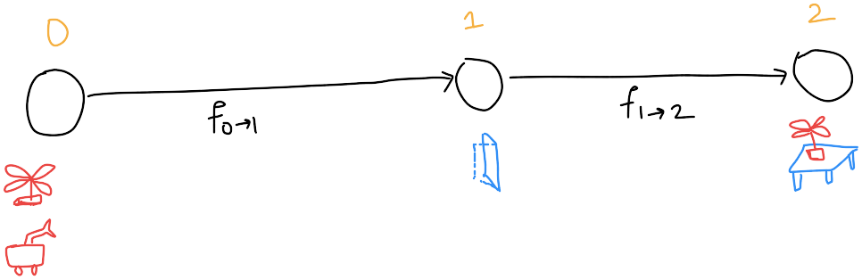
Figure 2: Aerial and ground robot task

• Two Species of robots: aerial robot and ground robot

• Reward Functions $r_{j}$ (Task node $j$)

• Heterogeneous Flow: $f_{j\rightarrow k}\in\mathbb{R}^{2}$ (for each species)

The reward functions for each task:

$$r_{1} =\begin{cases}1,~{}~{}\text{if}~{}~{}f_{0\rightarrow 1}\geq\begin{bmatrix}1\\ 1\end{bmatrix}\\ 0,~{}~{}\text{otherwise}\end{cases}$$

$$r_{2} =r_{1}\left(\begin{bmatrix}1&0\end{bmatrix}f_{1\rightarrow 2}\right)$$

MinCost Flow Problem:

$$\max_{f_{0\rightarrow 1},f_{1\rightarrow 2}}\sum_{(j,k)\in E}r_{1}\left(f_{0\rightarrow 1}\right)+r_{2}\left(f_{1\rightarrow 2},r_{1}\right)$$ (1)

More Generally:

$$\max_{f}\sum_{(j,k)\in E}r_{k}\left(\{f_{j\rightarrow k},r_{j}\}\right)$$ (2)

1.1.1 State Dependent Performance Functions for the tasks

1.2 Homogeneous, with branches

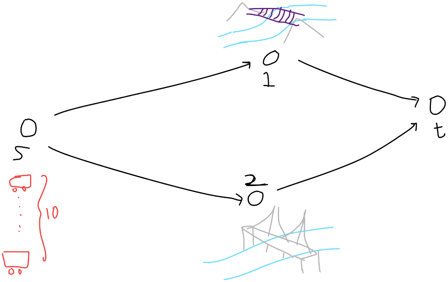
Figure 3: Ground robots must cross river—rickety bridge which can only carry a few robots and a strong bridge that can carry all robots but must be farther away

• One Species of robots: ground robot

• Reward Functions $r_{j}$ (Task node $j$)

• Heterogeneous Flow: $f_{j\rightarrow k}\in\mathbb{R}$

The reward functions for each task:

$$r_{1} =\begin{cases}100.0\times f_{s\rightarrow 1},~{}~{}\text{if}~{}~{}f_{0\rightarrow 1}\leq 4\\ -\infty,~{}~{}\text{otherwise}\end{cases}$$

$$r_{2} =0.01\times f_{s\rightarrow 2}$$

MinCost Flow Problem:

$$\min_{f_{s\rightarrow 1},f_{s\rightarrow 2}}\sum_{(j,k)\in E}r_{1}\left(f_{s\rightarrow 1}\right)+r_{2}\left(f_{s\rightarrow 2}\right)$$ (3)

2 What can flow model?

Some main truths about flow, and the respective consequences:

• Flow is conserved. In our problems, the team of robots is what is conserved; therefore, our flow is robots.

• Flow is trivial in simple line graphs. Therefore, modeling task graphs as flow is useful for complex task graphs that contain many splits/branches.

Based on the second item listed here, we must understand what causes splits (multiple outgoing edges) in a task graph and we must understand the characteristic/properties of branches converging (multiple incoming edges).

2.1 Splits

A single task precedence, or cascading precedences (e.g., A must precede B, which must precede C), create a chain task graph (like Figure 2). In order for splits to occur in a task graph, there must be one of two main types of precedences: an OR precedence, and an AND precedence.

Figure 4: Task graphs can have splits when a set of preceding tasks must all be done but there is no constraint on the order in which they are done (‘AND’), or when any single task within a set of preceding tasks must be completed (‘OR’).

2.1.1 AND Splits

If order impacts the amount of reward, then it is meaningful to model this split, and meaningful to send robots down different branches. If order does not matter (e.g., no impact on rewards, performance, etc.), then it the set of tasks within this AND precedence can be combined into a single task node.

The diagram in Figure 4 is not the only way to model the AND split. Below, Figure 5 shows two possible models.

The left model has a branch for each permutation. For a single agent flowing through, this model works well. However, if multiple robots flow through, there is overlap that isn’t accounted for. For example, imagine a flow of two robots that splits up among these branches. Robot one completes task A and then moves on to task B. However, when it gets to B, these could theoretically already be completed by robot two (and the same for when robot two moves on to completing task A).

The right model has a branch for each node in the set with edges between each. For multiple agents that are split among the edges, this might better capture different tasks being completed in parallel, however, the sink node must somehow measure/observe whether all the required tasks have been completed. For example, if all flow goes though A then B then to the sink, there is no flow in the A-Sink edge, but all the required tasks have been completed.

For both models, even small sets of AND tasks blow up the size of the task graph quickly (because of the permutations). In the left model, the number of branches explodes, while in the right model, the number of branches grows linearly but the edges between all these branches explodes.

Figure 5: Two potential models of the AND split. The left contains a branch for every permutation, whereas the right has a branch for each task with connecting edges between the nodes.

2.1.2 OR Splits

The OR splits seem to be well behaved. Edges in between branches could allow for adaptive planning (e.g., agents would complete another task withing the OR set if the prior task performance was poor). However, the number of these edges would explode as the number of tasks in the OR set grow.

Similar to the AND splits, there are difficulties modeling tasks being completed in parallel. For example, if two robots split between A and B, but then the first robot decides to additionally complete B (maybe because it did poorly on A), how are the rewards reflected? And does the model reflect this?

2.2 Convergence

Nodes where multiple branches converge must account for this set of influences. As noted in the prior section, this will depend on the structure of the splits. While the number of incoming edges to a convergence node is fixed, there is not necessarily flow coming from all edges. Therefore, I expect convergence nodes will need to use aggregate functions (e.g., max, min, avg, sum).

2.3 Alternatives to Flow

One of the main limitations of modeling our robots as units of flow through a graph is that the order in which they execute tasks must be the order of task dependence. An edge A $\rightarrow$ B only exists if task A precedes task B and influences task B’s reward, so a robot can only perform task B after task A if those conditions hold true. But it might be advantageous for a robot to perform task B after task A when the two are unrelated, such as when A and B are nearby one another and require the same capabilities.

There are a number of alternative formulations that rely on the same graph structure but do not model robot assignment as flow. These formulations might allow us to work around this issue. We would lose any benefits from using flow algorithms, but are we using these algorithms anyway?

1. Perform “iterative” flow where we re-assign robots to nodes and then re-solve and take a step of the flow solution at each iteration. If we can get the flow solution to be relatively fast, we could avoid the issue of robots being stuck along the path of task precedence by re-assigning the robots at each step. With homogeneous robots, an iteration would go like this:

   1. Calculate cost of flow given the current assignment of robots to tasks, $c_{old}$. This means trimming the graph of completed tasks, putting source nodes where the robots are currently assigned, and solving min cost flow for the remaining portion of the graph.

   2. Calculate cost of new flow, with a different assignment of robots to tasks, $c_{new}$. This corresponds to solving the same flow problem with different source nodes or values at source nodes.

   3. Perform 1-to-1 assignment to decide the optimal reassignment of robots to tasks from old flow to new flow. The assignment costs will be based on the cost of the robot to travel from the site of the old assignment to the site of the new assignment. Then, we only perform the re-assignment if the total cost of this 1-to-1 assignment is less than $c_{old}-c_{new}$, the marginal benefit of re-assigning.

   This brings up a few questions. First, how do we find candidates for new flow source node numbers? Candidates could be the new solution to the untrimmed flow problem (i.e. using the whole original graph with all the completed tasks still on it), but does this violate any assumptions? Second, when is this really useful? When there is significant benefit from robots completing tasks not in the order of precedence. Could this also enable disjoint sets of tasks to be considered for the same robot team?

   Note: this approach could be really really slow. If so, it could be used to generate training data that we then use for imitation learning for a value-function estimator to speed it up.

2. Add “dashed” edges to the graph which do not convey precedence/influence and generate a policy by which robots choose edges to navigate along based on the underlying graph structure.

   Perhaps the principal challenge in this alternative is assigning a proper cost to these edges - how can this cost be assigned to a node so that it is factored in to the overall system reward? This framework might function better as a ”value function” sort of problem, where robots collect rewards at tasks (the same task reward functions would be used) but also costs along edges that belong to the robot or group of robots, not the system as a whole.

3. Compute an assignment via node embedding. Using a GNN or other method for computing node embedding (??) we could take the task graph as input and not even reason about the robots navigating along the task graph. Instead, we could compute an embedding of the graph which labels each node according to which robot(s) the task is assigned. The principal challenge in this alternative is determining the order in which robots complete the tasks they are assigned.

4. Others??

2.4 Summary

2.4.1 Interactions our model can capture

1. Pure precedence

2. “OR” precedence

3. “AND” precedence (both AND and OR can be encoded via conditions embedded in the merging node)

2.4.2 Interactions our model cannot capture

1. Switching branches while already on a branch (what is the formal way to say this?)

   1. If we apply the flow solution iteratively, re-calculating as we receive new information, we could re-assign agents at each iteration. This would initialize them on different branches, effectively allowing them to ”switch.”

2. Impact to tasks that robots are not flowing through (ghost rewards)

3. single robot multi-task (can be addressed by dissolving into the same task node but goes against the principle of atomic tasks)

3 Modeling Task Rewards

The task rewards are a composition of two functions:

• coalition function (characteristic function $\rho(\cdot):\mathbb{R}^{k}\rightarrow\mathbb{R}$, where $k$ is the number of classes of agents. This maps a representation of the quantity and types of agents working on a task to the task performance. Maybe we parameterize it as a function drawn from the basis linear, sublinear, step

• “influence” function $\delta(\cdot):\mathbb{R}^{l}\rightarrow\mathbb{R}$, where $l$ is the number of sending neighbor nodes (the number of nodes whose rewards impact the current node’s reward). This function takes in the rewards received at influencing tasks, and maps it to task performance.

  Maybe this ranges from [0,1) and is a degradation of the coalition function, which represents the max theoretical performance of a coalition on a task.

This must be a non-linear function in order to encode “soft” precedence constraints, wherein a performance below a certain value on a preceding task zeroes out all future task rewards. In order for the function to express this, it cannot be a linear combination of coalition terms and preceding task performance terms.

A good candidate function format might be $r_{u}=\rho_{u}\delta_{u}$

3.1 Modeling Uncertainty

We want to represent the rewards at the tasks as some probability distribution to reflect the uncertainty in task completion. We want this uncertainty model to be:

1. Updateable: We are interested in updating our estimates of task PDFs in a number of ways:

   • With a Bayesian update rule incorporating our prior estimate and new observations either (1) during execution, or (2) from prior runs of the whole system

   • With new information that comes from a lower-level representation of the task. This could be something like the MDP-based tasks presented in cite: Aaron Ames paper

   • Are these two update rules mutually exclusive?

   Do we want to update the PDF estimate across robot coalitions? For example, if a team of four robots performs poorer than expected on a task, should we discount the expected reward for a team of 5 robots executing the task?

2. A function of robot coalition and of preceding task performance. as described above

3.2 Assumptions

We can leverage our knowledge about the functions that determine our task rewards to create smarter update rules. What can we assume that we know beforehand about our task rewards?

• Coalition function: the coalition function might be reasonable to know beforehand. This is like knowing that we’ll need four robots to lift the couch, or two robots to stabilize a beam, or that our coverage performance will increase sublinearly with number of agents. What happens if we make this assumption and then it turns out we need five robots to lift the couch rather than four? We may give up on the task when the correct solution is to allocate another robot to it.

3.3 Candidate Models

3.3.1 Mean-variance Noise

Here, $w$ represents independent Gaussian noise.

• Additive noise in the constituent functions:
  

  $$\bar{\rho}=\rho+w_{\rho}\;\;,\;\;\bar{\delta}=\delta+w_{\delta}\;\;,\;\;r_{u}=\bar{\rho}_{u}\bar{\delta}_{u}$$

• Multiplicative noise in the constituent functions:
  

  $$\bar{\rho}=w_{\rho}\rho\;\;,\;\;\bar{\delta}=w_{\delta}\delta\;\;,\;\;r_{u}=\bar{\rho}_{u}\bar{\delta}_{u}=w_{\rho}w_{\delta}\rho\delta$$

• Additive noise after the constituent functions:
  

  $$r_{u}=\rho_{u}\delta_{u}+w_{u}$$

3.3.2 Conditional Probability

Our network is very similar to a Bayesian network. A Bayesian network is a directed, acyclic graph (DAG) in which directed edges indicate conditional dependence between nodes. For example, if node $A$ is connected to node $B$ then $P(B|A)\neq P(B)$. Conversely, if two nodes are not connected, then they are conditionally independent. This fits with our assumptions of task reward influence.

In a Bayesian network, each node $B$ has an associated probability density function $p(B|A_{1},A_{2},...,A_{n})$ where $\{A_{1}...A_{n}\}$ are the set of nodes with incoming edges to $B$ i.e. the nodes that influence $B$. In our system, we’d have an additional dependence on the coalition function of the set of robots flowing through the node: $p(B|A_{1},A_{2},...,A_{n},\rho(f_{B}))$

This conditional probability can be used in a Bayes filter (or Kalman filter, if we can figure out how to make everything a Gaussian distribution). We would use only the “update” step of the typical “update, predict” filter process. This step is as follows:

$$p(x_{k}|z_{1:k})=p(z_{k}|x_{k})p(x_{k}|z_{1:k-1})$$

Here, $p(x_{k}|z_{1:k})$ is the current estimate of the node’s probability density function. $p(z_{k}|x_{k})$ is the measurement model, so we may assume it is some constant, or the likelihood of the observed reward ($z_{k}$) in the $k-1$th probability density function. And $p(x_{k}|z_{1:k-1})$ is the $k-1$th estimate of the probability density function. This expression should also be normalized.

A good place to start might be to make sure all of our probability density functions are Gaussian, and then perform the Kalman filter update step.

4 Next Steps

• Analyze the computational cost of our task graph. Does the “cascading” nature of our reward function for each node make it poorly suited for MILP? What size problem (size measured by number of tasks, because our system is agnostic to number of agents) can MILP solve in a reasonable time frame?

5 Dynamic Programming Approach

Let $\mc{T}:=\{\mc{T}_{1},\ldots,\mc{T}_{M}\}$ represent the set of $M$ available tasks in the environment, and $\mc{M}:=\{1,\ldots,M\}$ represent the index set of tasks. If task $\mc{T}_{j}$ must be performed before task $\mc{T}_{k}$ (e.g., opening and moving through a door before surveilling a room), we represent this relationship via a directed edge $(j,k)$ from task $\mc{T}_{j}$ to task $\mc{T}_{k}$. This leads to the representation of the overall mission as a task graph and the execution of tasks by robots as particular flows through the graph.

Given a set of $M$ tasks, let $\mc{G}_{T}=(\bar{\mc{M}},\mc{E})$ be a directed graph representing the relationships and dependencies among the tasks that must be executed as part of the overall multi-robot mission, where $\bar{\mc{M}}=\{0,1,2,\ldots,M+1\}$ is the vertex set and $\mc{E}$ is the corresponding edge set. While vertex $1,\ldots,M$ represent the actual tasks, vertex $0$ and $M$ represent a virtual “source” and “sink” node, respectively, as illustrated in Fig. LABEL:. The presence of a directed edge $(j,k)$ in $\mc{E}$ indicates the dependence of the execution of task $\mc{T}_{k}$ on the execution of task $\mc{T}_{j}$. Note that, if $(j,k)\in\mc{E}$ then $k>j$.

Let $f_{jk}\in\mc{R}$ represent the population fraction of robots transitioning from task $j$ to task $k$, associated with the edge $(j,k)$. Let $r_{j}$ denote the reward obtained at task node $j$ after executing task $\mc T_{j}$. This reward depends on two factors: the cumulative incoming flow into node $j$ (denoted as $f_{\rightarrow j}$) but also the rewards in the source nodes corresponding to the incoming edges. Simply, this relationship can be written as follow reward dynamics:

$$r_{j}=\mc{R}_{j}\left[f_{\rightarrow j},~{}\{r_{k}\}_{k\in\mc N_{j}^{in}}\right]$$ (4)

Our overall objective is to minimize the negative reward at all the task nodes (ignoring CVaR and the stochastic component for now):

$$\min_{f} \sum_{i=1}^{M}r_{i}^{2}$$ (5)

s.t. $$r_{j}=\mc{R}_{j}\left[f_{\rightarrow j},~{}\{r_{k}\}_{k\in\mc N_{j}^{in}}\right]$$ (6)

This is essentially an optimal control problem. We can simplify it’s solution by deriving a recursion equation.

To this end, for $l=\{0,\ldots,N-1\}$, let $V_{l}=\{0,\ldots,l\}$ denote a set of vertices. $z_{l}=\{r_{l+1},\ldots,r_{M}\}$ denote the set of future re

6 Papers

The multi-visit team orienteering problem with precedence constraints

7