Abstract

An extension of the Standard Model with anomaly free $U(1)_{F}$ flavor symmetry is studied in this paper. With this extension and the addition of the right-handed neutrino states, the solution of anomaly free charge assignments is found, which gives appealing texture zero and hierarchical Yukawa matrices. This gives us a natural understanding of the hierarchies between charged fermion masses and Cabibbo-Kobayashi-Maskawa (CKM) matrix elements. Neutrino Dirac and Majorana coupling matrices also have desirable structures leading to successful neutrino oscillations with inverted neutrino mass ordering. Other interesting implications of the presented scenario are also discussed.

Keywords: Flavor symmetry; Fermion masses; Neutrino oscillations.

PACS numbers: 11.30.Hv, 12.15.Ff, 14.60.Pq

1 INTRODUCTION

Although being very successful, the Standard Model (SM) is unable to resolve some puzzles. Among them is a problem of fermion flavor. The origin of hierarchies between charged fermion masses and CKM mixing angles is unexplained. Moreover, the SM is unable to accommodate the neutrino data [1]. In this work we consider an extension that gives a simultaneous resolution of these problems. The extension, we consider is the flavor $U(1)_{F}$ symmetry, which will be gauged. Besides this, we augment the fermion sector with right-handed neutrinos (RHNs), which will be responsible for the generation of light neutrino masses and mixings.

While the Abelian flavor $U(1)_{F}$ is the simplest candidate for the flavor symmetry [2], its gauging is a challenging task because the anomaly cancelation conditions give severe constraints for realistic model building. Below we present our findings of the $U(1)_{F}$ charge assignment.

2 ANOMALY FREE FLAVOR $U(1)_{F}$

Earlier attempts to find an anomaly free setup with $U(1)_{F}$ symmetry, exist in the literature [3, 4, 5]. These have been either within the minimal supersymmetric extension of the SM [3] or within the supersymmetric grand unified theories (GUTs) [4, 5]. In [5] for the finding of the anomaly free $U(1)_{F}$ symmetries, extended GUT symmetry groups [unifying $SU(5)$ GUT and $U(1)_{F}$ (or some part of the latter)] has been used. Although this approach is very attractive, with unification putting additional constraints, it disallows us to have much texture zeros and predictions. Besides these, GUTs usually suffer other problems that are not directly related to the flavor symmetry. Since we feel that finding anomaly free $U(1)_{F}$ constructions is far from being fully explored, our study here will be SM extension with gauged $U(1)_{F}$ symmetry and RHN states.

The nontrivial states under the SM gauge group $G_{SM}=SU(3)_{c}\times SU(2)_{L}\times U(1)_{Y}$ that we introduce will be just those of the SM. These are the Higgs doublet $\varphi$ and three families of matter $\{q,u^{c},d^{c},l,e^{c}\}_{i=1,2,3}$ where $i=1,2,3$ is the family index. As far as the extension is concerned, the fermionic sector will be augmented with RHNs $N_{1,2,3\cdots}$. As already emphasized, the extra gauge symmetry $U(1)_{F}$ is considered, with the scalar field $X$ - the ”flavon” - needed for the $U(1)_{F}$ breaking.

For finding anomaly free $U(1)_{F}$ charges we will use several simple observations. First of all, recall that the simplest anomaly free $U(1)$ symmetry is the hypercharge symmetry $U(1)_{Y}$ - the part of the SM gauge sector. So, in principle for $U(1)_{F}$, the family dependent hypercharges can be used. Furthermore, by introducing the right-handed neutrinos one can also build the gauged $(B-L)$ symmetry, which is also anomaly free. Obviously, with family dependent $(B-L)$ charges, anomalies will still vanish. So, one option is to have $U(1)_{F}$’s charges $Q_{i}(f)$ as the following superposition $\bar{a}_{i}Y(f)+\bar{b}_{i}Q_{B-L}(f)$, where $\bar{a}_{i},\bar{b}_{i}$ are some constants. With this superposition, all anomalies of the $G_{SM}$ remain intact, and also following additional and mixed anomalies

$$(U(1)_{F})^{3}: ~{}~{}~{}~{}A_{111}=\sum_{i}Q_{i}^{3}~{},$$ (1a)

$$U(1)_{Y}\times(U(1)_{F})^{2}: ~{}~{}~{}~{}A_{Y11}=\sum_{i}Y_{i}Q_{i}^{2}~{},$$ (1b)

$$(U(1)_{Y})^{2}\times U(1)_{F}: ~{}~{}~{}~{}A_{YY1}=\sum_{i}Y_{i}^{2}Q_{i}~{},$$ (1c)

$$(SU(2)_{L})^{2}\times U(1)_{F}: ~{}~{}~{}~{}A_{221}=\sum_{i}\left[Q_{i}(l_{i})+3Q_{i}(q_{i})\right]~{},$$ (1d)

$$(SU(3)_{c})^{2}\times U(1)_{F}: ~{}~{}~{}~{}A_{331}=\sum_{i}\left[2Q_{i}(q_{i})+Q_{i}(u^{c}_{i})+Q_{i}(d^{c}_{i})\right]~{},$$ (1e)

$$({\rm Gravity})^{2}\times U(1)_{F}: ~{}~{}~{}~{}A_{GG1}=\sum_{i}Q_{i}~{}.$$ (1f)

automatically vanish. Although, for the $Q_{i}(f)$ assignments, the superposition $\bar{a}_{i}Y(f)+\bar{b}_{i}Q_{B-L}(f)$ can be considered, one immediate outcome is that, by requiring that the top quark has the renormalizable Yukawa coupling ($\lambda_{t}\sim 1$) with the Higgs doublet $\varphi$, the bottom quark and the tau lepton Yukawas will be allowed at renormalizable levels - with the expectancy that $\lambda_{b},\lambda_{\tau}\sim 1$. Besides this unpleasant fact, with only $\bar{a}_{i},\bar{b}_{i}$ we cannot get Yukawa coupling matrices with many texture zeros. Thus, for the $U(1)_{F}$’s charges we will consider the modified superposition

$$Q_{i}(f)=\bar{a}_{i}Y(f)+\bar{b}_{i}Q_{B-L}(f)+\Delta Q_{i}(f)~{},$$ (2)

where the additions $\Delta Q_{i}(f)$ will be selected in such a way that the anomalies $A_{YY1},A_{221},A_{331},A_{GG1}$ stay intact. However, for the vanishing of the anomalies $A_{111}$ and $A_{Y11}$ additional constraints on the charge prescriptions need to be imposed. It turns out that for this goal, instead of three RHNs, we will need four of them - $N_{1,2,3,4}$. The additions that satisfy these and give a desirable fermion pattern are

$$\Delta Q_{i}(q) =\bar{q}_{3}\{0,1,-1\}+\bar{q}_{8}\{1,1,-2\}~{},$$ (3a)

$$\Delta Q_{i}(u^{c}) =\bar{u}_{3}\{0,1,-1\}+\bar{u}_{8}\{1,1,-2\}~{},$$ (3b)

$$\Delta Q_{i}(d^{c}) =\bar{d}_{3}\{1,-1,0\}+\bar{d}_{8}\{1,1,-2\}~{},$$ (3c)

$$\Delta Q_{i}(l) =\bar{l}_{3}\{1,-1,0\}+\bar{l}_{8}\{1,1,-2\}~{},$$ (3d)

$$\Delta Q_{i}(e^{c}) =0~{},$$ (3e)

$$\Delta Q_{i}(N) =\bar{n}\{1,1,1,-3\}~{},$$ (3f)

​where $\{\cdots\}$ stand for diagonal matrices in flavor space and presented numbers are diagonal elements of the corresponding matrices. Note that, being traceless, these additions coincide with diagonal (Cartan) generators of $SU(3)$ [in Eqs. (3a)-(3d)] and $SU(4)$ unitary groups [in Eq. (3f)]. Thus the notations for the constants $(\bar{q}_{3,8},\cdots\!,\bar{l}_{3,8})$ become obvious. These constants, together with $\bar{a}_{i},\bar{b}_{i}$ will be enough for our purposes. Upon selecting these constants we will bear in mind some requirements that need to be satisfied in order to obtain desirable and phenomenologically viable model. These requirements are as follows:

(i) In order to have top quark Yukawa coupling $\lambda_{t}\sim 1$, the $U(1)_{F}$ symmetry should allow coupling $q_{3}u^{c}_{3}\varphi$ at a renormalizable level. At the same time, all other Yukawa terms (responsible for charged fermion masses) should emerge by spontaneous breaking of the $U(1)_{F}$. So, the adequate mass hierarchies and CKM mixings will be expressed by powers of $\langle X\rangle/M_{\rm Pl}$.

(ii) Dirac and Majorana-type couplings involving RHN $N$ states should be such that naturally generate light neutrino masses and mixings in order to accommodate recent neutrino data [1].

(iii) While the $U(1)_{F}$ charge assignment ansatz of Eqs. (2), (3) automatically ensure zero anomalies of (1c)-(1f), an additional constraints need to be imposed for canceling anomalies of (1a) and (1b).

(iv) Finally, the ratios of the states’ charges should be rational in order to allow (phenomenologically required) couplings between them.

Guided by these, in (2) we use normalization such that $Y(l)=1$ and $Q_{B-L}(q)=1/3,Q_{B-L}(l)=-1$. Also, without loss of any generality, for the scalar $X$, we will select $Q_{X}=1$. With these and requirements listed above, the best selection that we find is the following:

$$\bar{a}_{i}=\frac{1}{3}\{46,43,10\}~{},~{}~{}~{}\bar{b}_{i}=\frac{1}{3}\{-91,35,38\}~{},~{}~{}~{}$$

$$\{\bar{q}_{3},\bar{u}_{3},\bar{d}_{3},\bar{l}_{3}\}=\frac{1}{3}\{-16,7,-67/2,-3/2\}~{},$$

$$\{\bar{q}_{8},\bar{u}_{8},\bar{d}_{8},\bar{l}_{8}\}=\frac{1}{9}\{38,-41,23/2,51/2\}~{},~{}~{}~{}~{}\bar{n}=-\frac{5}{3}~{}.$$ (4)

With these, by using (2) and (3a)-(3f) we obtained the charges given in Table 1. One can readily check out that all anomalies given in (1a)-(1f) vanish. Note that after all charges are fixed, since whole Lagrangian respects $U(1)_{Y}$ symmetry, by making a family universal charge shift for the states $Q\to Q+\alpha Y$, all couplings and anomalies will remain intact. The constant $\alpha$ can be selected to have convenient form of the charges. We have already exploited this by setting $Q(q_{3})=0$ (see Table 1). Presented charge assignment give interesting textures for charged fermion mass matrices and neutrinos as well. These we discuss in the following sections.

3 QUARK AND CHARGED LEPTON YUKAWA TEXTURES

As mentioned, for the $U(1)_{F}$ gauge symmetry breaking, the SM singlet scalar $X$ - the flavon field - is introduced and its $U(1)_{F}$ charge is taken to be $Q_{X}=1$. The vacuum expectation value (VEV) $\langle X\rangle$ breaks the $U(1)_{F}$ and also forms fermion mass matrices. Since in the Yukawa couplings the appropriate powers of $\frac{X}{M_{\rm Pl}}$ and $\frac{X^{*}}{M_{\rm Pl}}$ will appear, it is convenient to introduce notations

$$\frac{X}{M_{\rm Pl}}\equiv\varepsilon~{},~{}~{}~{}~{}\frac{X^{*}}{M_{\rm Pl}}\equiv\bar{\varepsilon}~{}.$$ (5)

Note that $M_{\rm Pl}\simeq 2.4\times 10^{18}$ GeV is a reduced Planck scale, which will be treated as a natural cutoff for all higher dimensional nonrenormalizable operators.

With the $U(1)_{F}$ charges of the Higgs doublet $\varphi$ of $Q_{\varphi}=-7$, and of the fermion states given in Table 1, the $qu^{c}\varphi,qd^{c}\tilde{\varphi}$ and $le^{c}\tilde{\varphi}$ type couplings, involving different powers of $\varepsilon$ and $\bar{\varepsilon}$, will be:

Table 1: $U(1)_{F}$ charge ($Q$) assignment for the states. $Q_{X}=1$, $Q_{\varphi}=-7$.

$$\begin{array}[]{|c||c|c|c|c|c|c|}\hline\cr\vspace{-0.3cm}\hfil&&&&&&\\ \par\vspace{-0.4cm}\hfil&\{q_{1},q_{2},q_{3}\}&\!\{u^{c}_{1},u^{c}_{2},u^{c}_{3}\}\!&\!\{d^{c}_{1},d^{c}_{2},d^{c}_{3}\}\!&\!\{l_{1},l_{2},l_{3}\}\!&\!\{e^{c}_{1},e^{c}_{2},e^{c}_{3}\}\!&\!\!\{N_{1},N_{2},N_{3},N_{4}\}\!\!\\ &&&&&&\\ \hline\cr\vspace{-0.3cm}\hfil&&&&&&\\ \vspace{-0.3cm}Q&\!\{-11,-2,0\}\!&\{26,13,7\}&\!\{\!-10,\!-1,\!-9\}\!&\!\{48,6,-15\}\!&\!\!\{-61,\!-17,6\}\!\!&\{-32,10,11,5\}\\ &&&&&&\\ \hline\cr\end{array}$$

$$\left(\!\!\begin{array}[]{ccc}q_{1},&\!\!q_{2},&\!\!q_{3}\\ \end{array}\!\!\right)\!\!\left(\!\begin{array}[]{ccc}\overline{\varepsilon}^{8}&\varepsilon^{5}&\varepsilon^{11}\\ \overline{\varepsilon}^{17}&\overline{\varepsilon}^{4}&\varepsilon^{2}\\ \overline{\varepsilon}^{19}&\overline{\varepsilon}^{6}&1\\ \end{array}\!\right)\!\!\left(\!\!\begin{array}[]{c}u^{c}_{1}\\ u^{c}_{2}\\ u^{c}_{3}\\ \end{array}\!\!\right)\!\!\varphi+\left(\!\!\begin{array}[]{ccc}q_{1},&\!\!q_{2},&\!\!q_{3}\\ \end{array}\!\!\right)\!\!\left(\!\begin{array}[]{ccc}\varepsilon^{14}&\varepsilon^{5}&\varepsilon^{13}\\ \varepsilon^{5}&\overline{\varepsilon}^{4}&\varepsilon^{4}\\ \varepsilon^{3}&\overline{\varepsilon}^{6}&\varepsilon^{2}\\ \end{array}\!\right)\!\!\left(\!\!\begin{array}[]{c}d^{c}_{1}\\ d^{c}_{2}\\ d^{c}_{3}\\ \end{array}\!\!\right)\!\!\tilde{\varphi}~{}+$$

$$\left(\!\!\begin{array}[]{ccc}l_{1},&\!\!l_{2},&\!\!l_{3}\\ \end{array}\!\!\right)\!\!\left(\!\begin{array}[]{ccc}\varepsilon^{6}&\overline{\varepsilon}^{38}&\overline{\varepsilon}^{61}\\ \varepsilon^{48}&\varepsilon^{4}&\overline{\varepsilon}^{19}\\ \varepsilon^{69}&\varepsilon^{25}&\varepsilon^{2}\\ \end{array}\!\right)\!\!\left(\!\!\begin{array}[]{c}e^{c}_{1}\\ e^{c}_{2}\\ e^{c}_{3}\\ \end{array}\!\!\right)\!\!\tilde{\varphi}~{}+{\rm h.c.}$$ (6)

In front of each operator of (6) the dimensionless coupling (omitted here) should stand. Substituting the VEVs $\langle\varepsilon\rangle=\langle\overline{\varepsilon}\rangle\equiv\epsilon$, and omitting those terms, with high powers of $\epsilon$, which are irrelevant in practice, the Yukawa matrices $Y_{U},Y_{D},Y_{E}$ corresponding to up, down quarks, and charged leptons, respectively, are

$$Y_{U}\simeq\left(\begin{array}[]{ccc}a_{1}^{\prime}\epsilon^{8}&~{}~{}a_{1}\epsilon^{5}&~{}~{}0\\ 0&~{}~{}a_{2}\epsilon^{4}&~{}~{}\epsilon^{2}\\ 0&~{}~{}0&~{}~{}1\end{array}\right)\lambda_{t}^{0}~{},$$ (7)

$$Y_{D}\simeq\left(\begin{array}[]{ccc}e^{-i\eta_{1}}&~{}~{}0&~{}~{}0\\ 0&~{}~{}e^{-i\eta_{2}}&~{}~{}0\\ 0&~{}~{}0&~{}~{}1\end{array}\right)\!\cdot\!\left(\begin{array}[]{ccc}0&~{}~{}b_{1}\epsilon^{3}&~{}~{}0\\ b_{1}^{\prime}\epsilon^{3}&~{}~{}b_{2}\epsilon^{2}&~{}~{}b_{2}^{\prime}\epsilon^{2}\\ 0&~{}~{}0&~{}~{}1\end{array}\right)\!\!\kappa_{b}\epsilon^{2}~{}.$$ (8)

$$Y_{E}\simeq\left(\begin{array}[]{ccc}c_{1}\epsilon^{4}&~{}~{}0&~{}~{}0\\ 0&~{}~{}c_{2}\epsilon^{2}&~{}~{}0\\ 0&~{}0&~{}~{}1\end{array}\right)\!\!\kappa_{\tau}\epsilon^{2}~{}.$$ (9)

We have made field phase redefinitions in such a way that, in this basis, the CKM matrix is the unit matrix [it becomes nontrivial after the diagonalization of $Y_{U}$ and $Y_{D}$ of Eqs. (7) and (8), respectively]. Also, we have performed $1-3$ and $2-3$ rotation of $d^{c}$ states in such a way that $3-1$ and $3-2$ entries of $Y_{D}$ vanishes (this transformation of the $d^{c}_{1,2,3}$ states is unobservable in the SM). Moreover, $Y_{U}$ is real, two phases $\eta_{1,2}$ appear in $Y_{D}$, while $Y_{E}$ is real. The phases $\eta_{1,2}$ will not contribute to the quark masses, but will be important for the CKM matrix elements.

Starting with the quark sector, with proper (and fully natural) selection of input parameters we can get desirable values for fermion masses and CKM mixing angles. Since the Yukawa matrices are hierarchical, in a pretty good approximation we can derive the following analytic expressions:

$$\lambda_{t}=\lambda_{t}^{0}[1+{\cal O}(\epsilon^{4})]~{},~{}~{}~{}~{}\frac{\lambda_{u}}{\lambda_{t}}\simeq\frac{a_{1}^{\prime}\epsilon^{8}}{\sqrt{1+(a_{1}\epsilon/a_{2})^{2}}}~{},~{}~{}~{}~{}\frac{\lambda_{c}}{\lambda_{t}}\simeq a_{2}\epsilon^{4}\sqrt{1+(a_{1}\epsilon/a_{2})^{2}}~{},$$ (10)

$$\lambda_{b}=\kappa_{b}\epsilon^{2}[1+{\cal O}(\epsilon^{4})]~{},~{}~{}~{}~{}\frac{\lambda_{d}}{\lambda_{b}}\simeq\frac{b_{1}b_{1}^{\prime}\epsilon^{4}}{\sqrt{b_{2}^{2}+(b_{1}^{2}+b_{1}^{\prime 2})\epsilon^{2}}}~{},~{}~{}~{}~{}\frac{\lambda_{s}}{\lambda_{b}}\simeq\epsilon^{2}\sqrt{b_{2}^{2}+(b_{1}^{2}+b_{1}^{\prime 2})\epsilon^{2}}~{}.$$ (11)

For writing down expression of the CKM matrix elements, it is useful to introduce two angles

$$\tan\theta_{u}=\frac{a_{1}}{a_{2}}\epsilon\sqrt{1+\epsilon^{4}}~{},~{}~{}~{}~{}\tan 2\theta_{d}=\frac{2b_{1}b_{2}\epsilon\sqrt{1+b_{2}^{\prime 2}\epsilon^{4}}}{b_{2}^{2}-(b_{1}^{2}-b_{1}^{\prime 2})\epsilon^{2}}~{},$$ (12)

and notations $\sin\theta_{u,d}\equiv s_{u,d}$ and $\cos\theta_{u,d}\equiv c_{u,d}$. With these we have

$$|V_{us}|=\left|c_{u}s_{d}e^{i\eta_{1}}-s_{u}c_{d}\frac{(e^{i\eta_{2}}+b_{2}^{\prime}\epsilon^{4})}{\sqrt{1+\epsilon^{4}}\sqrt{1+b_{2}^{\prime 2}\epsilon^{4}}}\right|+{\cal O}(\epsilon^{7})~{},$$

$$|V_{cb}|=c_{u}\epsilon^{2}\frac{\left|1-e^{i\eta_{2}}b_{2}^{\prime}(1+b_{2}^{2}\epsilon^{4})\right|}{\sqrt{1+\epsilon^{4}}\sqrt{1+b_{2}^{\prime 2}\epsilon^{4}}}+{\cal O}(\epsilon^{8})~{},~{}~{}~{}~{}~{}~{}\frac{|V_{ub}|}{|V_{cb}|}=\tan\theta_{u}~{}.$$ (13)

For the parameter

$$\overline{\rho}+i\overline{\eta}=-\frac{V_{ud}V_{ub}^{*}}{V_{cd}V_{cb}^{*}},$$ (14)

related to the $CP$ violation and defined in a phase convention independent way [10], we obtain

$$\overline{\rho}+i\overline{\eta}\simeq\frac{c_{u}c_{d}e^{i\eta_{1}}+s_{u}s_{d}e^{i\eta_{2}}}{c_{d}s_{u}e^{i\eta_{1}}-c_{u}s_{d}e^{i\eta_{2}}}\tan\theta_{u}.$$ (15)

Upon parametrization of the Yukawa matrices we have taken away the factors $\lambda_{t}^{0}$ and $\kappa_{b}$. These will be selected in such a way as to get observed values of masses $M_{t}$ and $m_{b}$. Remaining parameters (i.e. $\epsilon,a_{1,2},a_{1}^{\prime},b_{1,2},b_{1,2}^{\prime},\eta_{1,2}$) will determine light quark masses and CKM matrix elements. Relations (10)-(13) and (15) will help to find parameters giving desirable fit. Before going to that, let us mention that all quantities (output observable), obtained at high scale $\Lambda$ (which we take close to the GUT scale - few$\times 10^{16}$ GeV), need to be renormalized at low energies. For this we perform the renormalization and calculate these quantities at low scales. We have

$$\left.\frac{\lambda_{u,c}}{\lambda_{t}}\right|_{M_{t}}=\eta_{u,c}\left.\frac{\lambda_{u,c}}{\lambda_{t}}\right|_{\Lambda}~{},~{}~{}~{}\left.\frac{\lambda_{d,s}}{\lambda_{b}}\right|_{M_{t}}=\eta_{d,s}\left.\frac{\lambda_{d,s}}{\lambda_{b}}\right|_{\Lambda}~{},~{}~{}~{}$$

$$\left.V_{\alpha\beta}\right|_{M_{Z}}=\eta_{mix}\left.V_{\alpha\beta}\right|_{\Lambda}~{},~{}~{}~{}{\rm if}~{}~{}~{}(\alpha\beta)=(ub,cb,td,ts)~{},$$

$$\left.V_{\alpha\beta}\right|_{M_{Z}}=\left.V_{\alpha\beta}\right|_{\Lambda}~{},~{}~{}~{}{\rm if}~{}~{}~{}(\alpha\beta)=(ud,us,cd,cs,tb)~{}.$$ (16)

In one-loop approximation we have $\eta_{u,c}\simeq 1/\eta_{d,s}\simeq 1/\eta_{mix}\simeq\exp\!\left(\!\frac{3}{32\pi^{2}}\!\!\int_{\!M_{t}}^{\Lambda}\lambda_{t}^{2}d\ln\mu\!\right)$. However, we will perform more accurate calculations. For the renormalization of the light family Yukawa couplings and $\lambda_{b,\tau}$ we use two-loop renormalization group (RG) equations, while the runnings of $\lambda_{t}$ and $g_{3}$ are performed through three-loop RGs. For the running of the CKM matrix elements the two-loop RGs [6] will be used. Upon the running between $M_{t}$ (the pole mass of the top quark) and the scale $\Lambda$, for boundary values of the couplings at $\mu=M_{t}$ we use values given in [7].

Doing so, for $M_{t}=172.5$ GeV and $\alpha_{3}(M_{Z})=0.1179$ (the values we use throughout of this work) we get

$$\eta_{u,c}\simeq 1.1262+0.00187\cdot\ln\!\left(\!\frac{\Lambda}{2\!\cdot\!10^{16}{\rm GeV}}\!\right),$$ (17)

$$\eta_{d,s}\simeq 0.8916-0.00143\cdot\ln\!\left(\!\frac{\Lambda}{2\!\cdot\!10^{16}{\rm GeV}}\!\right),$$ (18)

$$\eta_{mix}\simeq 0.89157-0.001433\cdot\ln\!\left(\!\frac{\Lambda}{2\!\cdot\!10^{16}{\rm GeV}}\!\right),$$ (19)

which are the interpolated expressions that work pretty well for $10^{15}{\rm GeV}\!<\!\Lambda\!<\!M_{\rm Pl}$.

Also, for light quark masses, the running from $M_{t}$ down to low scales need to be performed by the standard technics [7, 8, 9].

A. Fit for charged Fermion masses and CKM elements

A good fit is obtained for the following values of input parameters (values are given at high scale $\Lambda=2\times 10^{16}$ GeV):

$$\epsilon=0.21,~{}~{}\{a_{1},a_{1}^{\prime},a_{2}\}=\{0.6974,~{}1.7065,~{}1.6606\},~{}~{}\{\eta_{1},\eta_{2}\}=\{3.01985,~{}-1.3954\},$$

$$\{b_{1},b_{1}^{\prime},b_{2},b_{2}^{\prime}\}=\{0.47834,~{}0.54541,~{}0.45448,~{}0.59088\}.$$ (20)

These, by performing renormalization [using (16)-(19) and input $M_{t}=172.5$ GeV, $m_{b}(m_{b})=4.18$ GeV], at low scales give

$$\left(m_{u},~{}m_{d},~{}m_{s}\right)(2~{}{\rm GeV})=\left(2.16,~{}4.67,~{}93\right){\rm MeV},~{}~{}~{}m_{c}(m_{c})=1.27~{}{\rm GeV}~{},$$

$${\rm at}~{}~{}\mu=M_{Z}:~{}~{}|V_{us}|=0.225,~{}~{}|V_{cb}|=0.04182,~{}~{}|V_{ub}|=0.00369,~{}~{}~{}\overline{\rho}=0.159,~{}~{}\overline{\eta}=0.3477,$$ (21)

where definitions for $\overline{\rho},\overline{\eta}$ are given in Eq. (14). All results given above are in perfect agreement with experiments [10].

As far as the charged lepton masses are concerned, from (9) with the input $M_{\tau}=1.777$ GeV and

$${\rm at}~{}~{}\mu=\Lambda~{},~{}~{}~{}~{}\{c_{1},c_{2}\}\simeq\{0.1437,1.335\},$$ (22)

and taking into account that $\left.\frac{\lambda_{e,\mu}}{\lambda_{\tau}}\right|_{M_{Z}}\!\!\cong\!\left.\frac{\lambda_{e,\mu}}{\lambda_{\tau}}\right|_{\Lambda}$, we obtain

$$M_{e}=0.511~{}{\rm MeV},~{}~{}~{}~{}M_{\mu}=105.66~{}{\rm MeV},$$ (23)

which is also in agreement with experiments.

4 NEUTRINO SECTOR

For building the realistic neutrino sector, the singlet states $N_{1,2,3}$ will be used as right-handed neutrinos. Since the $N_{4}$ is not really needed for these purposes, its couplings to the leptons and also to $N_{1,2,3}$ can be easily avoided by imposing the reflection symmetry $N_{4}\to-N_{4}$ (this symmetry and its possible implication will be commented on below). This will make the analysis simpler. Thus, with $U(1)_{F}$ charges given in Table 1 the $lN\varphi$ and $N_{i}N_{j}$ type couplings ($i,j=1,2,3$) will be

$$\left(\!\!\begin{array}[]{ccc}l_{1},&\!\!l_{2},&\!\!l_{3}\\ \end{array}\!\!\right)\!\!\left(\!\begin{array}[]{ccc}\overline{\varepsilon}^{9}&\overline{\varepsilon}^{51}&\overline{\varepsilon}^{52}\\ \varepsilon^{33}&\overline{\varepsilon}^{9}&\overline{\varepsilon}^{10}\\ \varepsilon^{54}&\varepsilon^{12}&\varepsilon^{11}\\ \end{array}\!\right)\!\!\left(\!\!\begin{array}[]{c}N_{1}\\ N_{2}\\ N_{3}\\ \end{array}\!\!\right)\!\!\varphi+\left(\!\!\begin{array}[]{ccc}N_{1},&\!\!N_{2},&\!\!N_{3}\\ \end{array}\!\!\right)\!\!\left(\!\begin{array}[]{ccc}\varepsilon^{64}&\varepsilon^{22}&\varepsilon^{21}\\ \varepsilon^{22}&\overline{\varepsilon}^{20}&\overline{\varepsilon}^{21}\\ \varepsilon^{21}&\overline{\varepsilon}^{21}&\overline{\varepsilon}^{22}\\ \end{array}\!\right)\!\!\left(\!\!\begin{array}[]{c}N_{1}\\ N_{2}\\ N_{3}\\ \end{array}\!\!\right)\!\!M_{\rm Pl}.$$ (24)

In these operators the dimensionless couplings are still omitted. Substituting the VEVs $\langle\varepsilon\rangle=\langle\overline{\varepsilon}\rangle=\epsilon$, $\langle\varphi\rangle=v$ and omitting irrelevant small entries, for neutrino Dirac and Majorana matrices we get

$$m_{D}\!\simeq\!\left(\begin{array}[]{ccc}A\epsilon^{9}&0&0\\ 0&B_{1}\epsilon^{9}&C_{1}\epsilon^{10}\\ 0&B_{2}\epsilon^{12}&C_{2}\epsilon^{11}\\ \end{array}\right)\!\!v,~{}~{}~{}M_{R}\!\simeq\!\left(\begin{array}[]{ccc}0&a\epsilon^{2}&d\epsilon\\ a\epsilon^{2}&b&c\epsilon\\ d\epsilon&c\epsilon&\epsilon^{2}\\ \end{array}\right)\!\!\bar{c}M_{Pl}\epsilon^{20}.$$ (25)

These lead to the light neutrino $3\times 3$ mass matrix:

$$\begin{array}[]{ccc}&{\begin{array}[]{ccc}&{}{}\hfil&{}{}\hfil\end{array}}\\ \vspace{1mm}\begin{array}[]{c}\\ {}\hfil\\ {}\hfil\end{array}\!\!\!\!\!&{\!M_{\nu}\simeq-m_{D}M_{R}^{-1}m_{D}^{T}\simeq\left(\begin{array}[]{ccc}\beta&~{}~{}\gamma&~{}~{}\gamma^{\prime}\\ \gamma&~{}~{}\alpha^{2}&~{}~{}\alpha\\ \gamma^{\prime}&~{}~{}\alpha&~{}~{}1\end{array}\right)\bar{m}},\end{array}\!\!~{}~{}~{}$$ (26)

with $\bar{m}$ and the dimensionless couplings $\alpha,\beta,\gamma,\gamma^{\prime}$ expressed by the scales and couplings appearing in Eq. (25). Note that $M_{\nu}$’s $2-3$ block’s determinant is zero:

$$M_{\nu}^{(2,2)}M_{\nu}^{(3,3)}-(M_{\nu}^{(2,3)})^{2}=0.$$ (27)

The origin of this relation can be understood as follows. Because of $M_{R}^{(1,1)}=0$, the determinant of the lower $2\times 2$ block of $M_{R}^{-1}$ is zero. Moreover, since the lower $2\times 2$ block of $m_{D}$ decouples [i.e., $(1,2)$ and $(1,3)$ entries in $m_{D}$ are zero] the seesaw formula $M_{\nu}\simeq-m_{D}M_{R}^{-1}m_{D}^{T}$ gives the relation of Eq. (27). The latter gives specific predictions, on which we will focus now.

Since the charged lepton mass matrix $Y_{E}$ is essentially diagonal, the whole lepton mixing matrix $U$ comes from the neutrino sector. Therefore, we have

$$M_{\nu}=PU^{*}P^{\prime}M_{\nu}^{\rm Diag}U^{{\dagger}}P,$$ (28)

where in a standard parametrization, $U$ has the following form:

$$U=\left(\begin{array}[]{ccc}c_{13}c_{12}&c_{13}s_{12}&s_{13}e^{-i\delta}\\ -c_{23}s_{12}-s_{23}s_{13}c_{12}e^{i\delta}&c_{23}c_{12}-s_{23}s_{13}s_{12}e^{i\delta}&s_{23}c_{13}\\ s_{23}s_{12}-c_{23}s_{13}c_{12}e^{i\delta}&-s_{23}c_{12}-c_{23}s_{13}s_{12}e^{i\delta}&c_{23}c_{13}\end{array}\right),$$ (29)

with $s_{ij}=\sin\theta_{ij}$ and $c_{ij}=\cos\theta_{ij}$. The phase matrices $P,P^{\prime}$ are given by

$$P={\rm Diag}\left(e^{i\omega_{1}}~{},~{}e^{i\omega_{2}}~{},~{}e^{i\omega_{3}}\right),~{}~{}~{}P^{\prime}={\rm Diag}\left(1~{},~{}e^{i\rho_{1}}~{},~{}e^{i\rho_{2}}\right),$$ (30)

where $\omega_{1,2,3},\rho_{1,2}$ are some phases.

As was investigated in details (see second Ref. in [5]), the relation (27) excludes the possibility of the normal ordering of the neutrino masses. Using Eqs. (28)-(30) in (27) the we obtain

$$e^{i\rho_{1}}m_{1}m_{2}s_{13}^{2}+e^{i(\rho_{2}+2\delta)}\left(m_{1}s_{12}^{2}+e^{i\rho_{1}}m_{2}c_{12}^{2}\right)m_{3}c_{13}^{2}=0,$$ (31)

which in turn gives

$$\cos\rho_{1}=\frac{m_{1}^{2}m_{2}^{2}\tan^{4}\theta_{13}-m_{3}^{2}(m_{1}^{2}s_{12}^{4}+m_{2}^{2}c_{12}^{4})}{2m_{1}m_{2}m_{3}^{2}s_{12}^{2}c_{12}^{2}},$$ (32)

$$2\delta=\pm\pi-\rho_{2}+{\rm Arg}\left(s_{12}^{2}e^{i\rho_{1}}+\frac{m_{2}}{m_{1}}c_{12}^{2}\right).$$ (33)

These two relations, together with measured values of $\Delta m_{\rm sol}^{2}$ and $\Delta m_{\rm atm}^{2}$ allow us to have only one free phase (out of the three phases $\delta,\rho_{1,2}$) and one free mass (out of the three light neutrino masses $m_{1,2,3}$). However, as we will see below, the latter’s range will turn out to be quite narrow.

Using recent results from the neutrino experiments [1], we can easily verify that the relation of Eq. (32) is incompatible with normal ordering of neutrino masses. On the other hand, inverted ordering of neutrino masses is possible. Using the best fit values (bfvs) of $\theta_{ij},\Delta m_{\rm sol}^{2}=m_{2}^{2}-m_{1}^{2}$, $\Delta m_{\rm atm}^{2}=m_{2}^{2}-m_{3}^{2}$, expressing $m_{1,2}$ by $m_{3}$ as $m_{1}\!=\!\sqrt{\Delta m_{\rm atm}^{2}\!-\!\Delta m_{\rm sol}^{2}\!+\!m_{3}^{2}}$, $m_{2}\!=\!\sqrt{\Delta m_{\rm atm}^{2}\!+\!m_{3}^{2}}$, from Eq. (32) we can get an allowed region for $m_{3}$:

$$0.001129~{}{\rm eV}\stackrel{{\scriptstyle<}}{{{}_{\sim}}}m_{3}\stackrel{{\scriptstyle<}}{{{}_{\sim}}}0.002833~{}{\rm eV}.$$ (34)

This implies $0.1002~{}{\rm eV}\stackrel{{\scriptstyle<}}{{{}_{\sim}}}\sum m_{i}\stackrel{{\scriptstyle<}}{{{}_{\sim}}}0.1021$ eV, satisfying the current upper bound $\sum m_{i}<0.12$ eV [11], which is obtained from cosmology.

Moreover, for neutrino less double $\beta$-decay ($0\nu\beta\beta$) parameter $m_{\beta\beta}=|\sum U_{ei}^{2}m_{i}P^{\!\!~{}^{\prime}\!*}_{i}|$ we obtain

$$m_{\beta\beta}=\left|c_{12}^{2}c_{13}^{2}m_{1}+s_{12}^{2}c_{13}^{2}m_{2}e^{i\rho_{1}}+s_{13}^{2}m_{3}e^{i(2\delta+\rho_{2})}\right|,$$ (35)

which taking into account Eqs. (32), (33) and bfvs of the oscillation parameters leads to:

$$0.01864~{}{\rm eV}\stackrel{{\scriptstyle<}}{{{}_{\sim}}}m_{\beta\beta}\stackrel{{\scriptstyle<}}{{{}_{\sim}}}0.0483~{}{\rm eV}.$$ (36)

This range is also compatible with limits provided by $0\nu\beta\beta$ experiments [12]. In fact, due to predictive relations in Eqs. (32), (33) both parameters $\sum m_{i}$ and $m_{\beta\beta}$ are unequivocally determined by the $m_{3}$ values. Thus, there is correlation between $\sum m_{i}$ and $m_{\beta\beta}$, which is given in Fig. 1. Hopefully, future experiments will be able to test viability of this scenario [13].

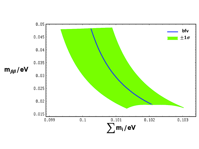
Figure 1: Correlation between $\sum m_{i}$ and $m_{\beta\beta}$. Solid (middle) blue line corresponds to the bfvs of the oscillation parameters [1]. Green (wider) area corresponds to the cases with oscillation parameters within the $1\sigma$ deviations.

Now we give one selection of the parameters, appearing in (25), which blends well with this neutrino scenario and then discuss some implications and outcomes. With the choice

$$\{a,b,c,d,\bar{c}\}\simeq\{3.2672e^{i1.5473},0.79405e^{i0.0053733},0.89097e^{i0.0028735},0.15853e^{1.5586},0.56333e^{2.9194}\},$$

$$\{A,B_{1},B_{2},C_{1},C_{2}\}\simeq\{2.0236,~{}2.0236,~{}1.6189,~{}2.4283,~{}-0.8094\},$$ (37)

for the light neutrino masses and mixing angles we obtain

$$\{m_{1},m_{2},m_{3}\}=\{0.049197,~{}0.049942,~{}0.0015\}{\rm eV},$$ (38)

$$\{\sin^{2}\theta_{12},\sin^{2}\theta_{23},\sin^{2}\theta_{13}\}=\{0.3035,~{}0.57,~{}0.02235\}.$$ (39)

From (38) we get

$$\Delta m_{\rm sol}^{2}=m_{2}^{2}-m_{1}^{2}=7.39\times 10^{-5}{\rm eV}^{2},~{}~{}\Delta m_{\rm atm}^{2}=m_{2}^{2}-m_{3}^{2}=2.492\times 10^{-3}{\rm eV}^{2}~{}.$$ (40)

Results of (39) and (40) correspond to the bfvs of the inverted ordering neutrino scenario [1]. Moreover, for the phases we get

$$\{\delta,\rho_{1},\rho_{2}\}=\{276^{\circ},~{}91.69^{\circ},~{}11.49^{\circ}\},~{}~{}~{}~{}\omega_{1,2,3}=0.$$ (41)

For this case we have $m_{\beta\beta}\simeq 0.0362$ eV and $\sum m_{i}\simeq 0.101$ eV. These certainly blend with the discussed predictions [of Eqs. (32), (33) and Fig. 1].

From the input (37) for the heavy RHN masses we get

$$\{M_{N_{1}},M_{N_{2}},M_{N_{3}}\}\simeq\{1.6,~{}953.5,~{}32480\}{\rm GeV}.$$ (42)

A few remarks about the heavy RHN sector are in order.

The state $N_{1}$ (with $M_{N_{1}}\simeq 1.6$ GeV) can be produced in decays of heavy mesons; however the corresponding mixing $|U_{eN_{1}}|^{2}\simeq 2.76\times 10^{-11}$ is a bit below (by factor of$\approx 3$) the sensitivity of the SHiP experiment [14]. As a separate study, it would be interesting to do a more detailed investigation/exploration of the model’s parameters from the perspective of this experiment.

Since the lightest RHN’s mass is $M_{N_{1}}\simeq 1.6$ GeV, and it mixes with $\nu_{e}$, there will be an additional contribution to the $02\beta\beta$ parameter, which is given by [15]

$$\left|\sum_{i=1}^{3}U_{ei}^{2}m_{i}P^{\!\!~{}^{\prime}\!*}_{i}+\frac{M_{N_{1}}}{1+M_{N_{1}}^{2}/\langle p^{2}\rangle}U_{eN_{1}}^{2}\right|=$$

$$\left|e^{-0.421i}0.0362~{}\!{\rm eV}+\frac{e^{-0.151i}2.76\cdot 10^{-11}M_{N_{1}}}{1+M_{N_{1}}^{2}/\langle p^{2}\rangle}\right|\!=\!0.0368~{}{\rm eV},~{}\left({\rm for}~{}\langle p^{2}\rangle\!=\!(200~{}\!{\rm MeV})^{2}\right).$$ (43)

The second term in the absolute values of Eq. (43) is the contribution from the $N_{1}$. The $\langle p^{2}\rangle$ is averaged momentum squared corresponding to this process. As can be seen, for $\langle p^{2}\rangle\!=\!(\!100\!-\!200~{}\!{\rm MeV})^{2}$ [15, 16] the correction from the $N_{1}$ state is within $(0.5\!-\!1.8)\%$, i.e. negligible. Therefore, the predictions, made from the light neutrino sector (and correlation of Fig. 1) are robust.

With $N_{1}$’s mass within the GeV scale, we need to ensure its sufficiently fast decay (within $\stackrel{{\scriptstyle<}}{{{}_{\sim}}}0.3$ sec.) in order to not affect the standard big bang nucleosynthesis (BBN). Dominant decays of $N_{1}$ are three body decays via neutral and charged currents (i.e., via $Z^{*}$ and $W^{*(\pm)}$ exchange). These are leptonic $N_{1}\to\nu_{i}\nu_{j}\bar{\nu}_{j},~{}\nu_{i}e^{-}_{j}e^{+}_{j},~{}e^{-}_{i}e^{+}_{j}\nu_{j}$ and semileptonic $N_{1}\to\nu_{i}q_{j}\bar{q}_{j},~{}e^{-}_{i}u_{j}\bar{d}_{k}$ decays. For the leptonic decay widths we use expressions given in Ref. [17]. For the semileptonic decays, taking into account all inclusive decays into the quarks, by proper use of the matching RG factor [18] one can get a quite reasonable estimate. Summing all kinematically allowed channels of $N_{1}$’s decays and using proper expressions [17, 18], for the total width (i.e., for inverse lifetime) we obtain

$$\Gamma(N_{1})=\frac{1}{\tau_{N_{1}}}\!\simeq\!\frac{G_{F}^{2}M_{N_{1}}^{5}}{16\pi^{3}}\!\left(\!1.37|U_{1N_{1}}|^{2}\!+\!1.35|U_{2N_{1}}|^{2}\!+\!0.487|U_{3N_{1}}|^{2}~{}\!\right)\simeq\frac{1}{0.0038~{}\!{\rm s.}}~{},$$ (44)

which is compatible with BBN. In Eq. (44), for the squared mixing matrix elements we have used values obtained within our model:

$$|U_{iN_{1}}|^{2}\simeq\{2.76,~{}1.29,~{}1.09\}\times 10^{-11},$$ (45)

which obtained from the inputs of (37). The states $N_{2,3}$ will decay much rapidly via the $N_{2,3}\to\varphi l$ channel (with lifetimes $\approx 7\times 10^{-3}$ ps and $2\times 10^{-4}$ ps respectively). As far as the state $N_{4}$ (which presence is important for anomaly cancelation) is concerned, because of the reflection symmetry $N_{4}\to-N_{4}$ (we have introduced), its mixing with $N_{1,2,3}$ and couplings to the SM leptons are forbidden. However, it will gain the mass via the $\frac{1}{2}M_{Pl}\bar{\varepsilon}^{10}N_{4}N_{4}$ operator: $M_{N_{4}}\sim M_{Pl}\epsilon^{10}\approx 4\times 10^{11}$ GeV. For its decay are responsible the operators

$$\frac{\lambda_{1}\bar{\varepsilon}}{M_{\rm Pl}^{2}}(N_{4}u^{c}_{3})(d^{c}_{1}d^{c}_{2})+\frac{\lambda_{2}\varepsilon}{M_{\rm Pl}^{2}}(N_{4}u^{c}_{2})(d^{c}_{1}d^{c}_{3})+{\rm h.c.},$$ (46)

which are allowed if all quarks also change sign. [I.e., $(q,u^{c},d^{c})\to-(q,u^{c},d^{c})$ under reflection symmetry. This does not affect the charged fermion and neutrino sectors.] These operators will give decays $N_{4}\to u^{c}_{3}d^{c}_{1}d^{c}_{2},~{}u^{c}_{2}d^{c}_{2}d^{c}_{3}$. Since $N_{4}$ is a Majorana state, also $N_{4}\to\bar{u}^{c}_{3}\bar{d}^{c}_{1}\bar{d}^{c}_{2},~{}\bar{u}^{c}_{2}\bar{d}^{c}_{2}\bar{d}^{c}_{3}$ decays will proceed. All these give $\Gamma(N_{4})\!=\!\frac{(|\lambda_{1}|^{2}+|\lambda_{2}|^{2})M_{N_{4}}^{5}\epsilon^{2}}{128\pi^{3}M_{\rm Pl}^{4}}\!=\!\frac{1}{10^{-4}{\rm sec.}}\left(\!\frac{M_{N_{4}}}{4\cdot 10^{11}{\rm GeV}}\!\right)^{\!5}$ (with $\lambda_{1,2}=1$), and therefore making $N_{4}$ harmless for the BBN. It would have been interesting to have a scenario with $N_{4}$ having proper value of mass and needed couplings for serving as a dark matter candidate. This turned out impossible with a presented $U(1)_{F}$ charge assignment. Perhaps a separate study focused on this issue is also worthwhile.

In summary, exploring the possibility of anomaly free gauged $U(1)_{F}$ flavor symmetry offered an attractive pattern for the charged fermion masses, neutrino oscillations, and also interesting phenomenological implications. These motivate us to think more and try to find other possibilities within the framework discussed in this work.

References

[1]
F. Capozzi, E. Di Valentino, E. Lisi, A. Marrone, A. Melchiorri and A. Palazzo,
Phys. Rev. D 104, 083031 (2021);
M. C. Gonzalez-Garcia, M. Maltoni and T. Schwetz,
Universe 7, 459 (2021).
[2]
C. D. Froggatt and H. B. Nielsen,
Nucl. Phys. B147, 277 (1979).
[3]
E. Dudas, S. Pokorski, and C. A. Savoy,
Phys. Lett. B 356, 45 (1995).
[4]
M. -C. Chen, D. R. T. Jones, A. Rajaraman, and H. -B. Yu,
Phys. Rev. D 78, 015019 (2008).
[5]
Z. Tavartkiladze,
Phys. Lett. B 706, 398 (2012);
Phys. Rev. D 87, 075026 (2013).
[6]
V. D. Barger, M. S. Berger, and P. Ohmann,
Phys. Rev. D 47, 2038 (1993).
[7]
S. P. Martin,
Phys. Rev. D 106, 013007 (2022).
See also references therein and Ref. [9] for the review and summary of RG equations.
[8]
H. Fusaoka and Y. Koide,
Phys. Rev. D 57, 3986 (1998).
[9]
Z. z. Xing, H. Zhang and S. Zhou,
Phys. Rev. D 77, 113016 (2008);
Z. z. Xing,
Phys. Rep. 854, 1 (2020).
[10]
R. L. Workman (Particle Data Group),
Prog. Theor. Exp. Phys. 2022, 083C01 (2022).
[11]
N. Aghanim et al. (Planck Collaboration),
Astron. Astrophys. 641, A6 (2020);
652, C4(E) (2021).
[12]
S. Abe et al. (KamLAND-Zen Collaboration),
arXiv:2203.02139.
[13]
K. N. Abazajian, N. Blinov, T. Brinckmann, M. C. Chen, Z. Djurcic, P. Du, M. Escudero, M. Gerbino, E. Grohs, S. Hagstotz et al.,
arXiv:2203.07377.
[14]
C. Ahdida et al. (SHiP Collaboration),
J. High Energy Phys. 04 (2019) 077.
[15]
M. Mitra, G. Senjanovic, and F. Vissani,
Nucl. Phys. B856, 26 (2012).
[16]
P. D. Bolton, F. F. Deppisch, and P. S. Bhupal Dev,
J. High Energy Phys. 03 (2020) 170.
[17]
A. Atre, T. Han, S. Pascoli, and B. Zhang,
J. High Energy Phys. 05 (2009) 030.
[18]
K. Bondarenko, A. Boyarsky, D. Gorbunov, and O. Ruchayskiy,
J. High Energy Phys. 11, (2018) 032, see also references therein.