L2xGnn: Learning to Explain Graph Neural Networks

Abstract

Graph Neural Networks (GNNs) are a popular class of machine learning models. Inspired by the learning to explain (L2X) paradigm, we propose L2xGnn, a framework for explainable GNNs which provides faithful explanations by design. L2xGnn learns a mechanism for selecting explanatory subgraphs (motifs) which are exclusively used in the GNNs message-passing operations. L2xGnn is able to select, for each input graph, a subgraph with specific properties such as being sparse and connected. Imposing such constraints on the motifs often leads to more interpretable and effective explanations. Experiments on several datasets suggest that L2xGnn achieves the same classification accuracy as baseline methods using the entire input graph while ensuring that only the provided explanations are used to make predictions. Moreover, we show that L2xGnn is able to identify motifs responsible for the graph’s properties it is intended to predict.

1 Introduction

Graph Neural Networks (GNNs) are a widely used class of machine learning models. Since graphs occur naturally in several domains such as chemistry, biology, and medicine, GNNs have experienced widespread adoption. Following a trend toward building more interpretable machine learning models, there have been numerous recent proposals to provide explanations for GNNs. Most of the existing approaches provide post-hoc explanations starting from an already trained GNN to identify edges and node attributes that explain the model’s prediction. However, as highlighted in Faber et al. [2021], there might be some discrepancy between the ground-truth explanations and those attributed to the trained GNNs. Indeed, post-hoc explanations are often not able to faithfully represent the mechanisms of the original model [Rudin, 2018]. Unfortunately, the very definition of what constitutes a faithful explanation is still open to debate and there exist several competing positions on the matter. Recent work has also shown that post-hoc attribution methods are often not better than random baselines on the standard evaluation metrics for explanation accuracy and faithfulness [Agarwal et al., 2022b]. Much fewer approaches have considered the problem of GNN explainability from an intrinsic perspective. In contrast to post-hoc methods, approaches with built-in interpretability provide explanations during training by introducing new mechanisms, e.g. prototypes [Zhang et al., 2021], stochastic attention [Miao et al., 2022], or graph kernels [Feng et al., 2022a]. Nonetheless, the introduction of new mechanisms to compute graph representations differ from standard GNNs computations. Therefore, the reasoning process of the above interpretable networks differ from the original GNN architectures making them not faithful by design. Our intent, instead, is to generate explanations for standard GNNs by keeping the computations as faithful as possible compared to the original network.

A recently proposed alternative to post-hoc methods is the learning to explain (L2X) paradigm [Chen et al., 2018]. The core difference to post-hoc methods is that the models are trained to, in the forward pass, discretely select a small subset of the input features as well as the parameters of a downstream model that uses only the selected features to make a prediction. The selected features are, therefore, faithful by design as they are the only ones used by the downstream model. Since the subset of features is sampled discretely, L2X requires a method for computing gradients of an expectation over a discrete probability distribution. Chen et al. [2018] proposed a gradient estimator based on a relaxation of the discrete samples and tailored to the $k$-subset distribution. However, since the original work only considers the case of selecting exactly-k features, directly applying prior methods to the graph learning tasks is not possible and requires significant changes.

With this work, we bring the L2X paradigm to graph representation learning. The important ingredient is a recently proposed method for computing gradients of an expectation over a complex exponential family distribution [Niepert et al., 2021]. The method facilitates approximate gradient backpropagation for models combining continuously differentiable GNNs with a black-box solver of combinatorial problems defined on graphs. Crucially, this allows us to learn to sample subgraphs with beneficial properties such as being connected and sparse. Contrary to prior work, this also creates a dependency between the random variables representing the presence of edges. The proposed framework L2xGnn, therefore, learns to select explanatory subgraph motifs and uses these and only these motifs for its message-passing operations. To the best of our knowledge, this is the first method for learning to explain on standard GNNs. The proposed framework is extensible as it can work with any optimization algorithm for graphs imposing properties on the sampled subgraphs.

We compare two different sampling strategies for obtaining sparse subgraph explanations resulting from two optimization problems on graphs: (1) the maximum-weight $k$-edge subgraph and (2) the maximum-weight $k$-edge connected subgraph problem. We show empirically that L2xGnn when combined with a base GNN does not lose accuracy on several benchmark datasets. Moreover, we evaluate the explanations quantitatively and qualitatively. We also analyze the ability of L2xGnn to help in detecting shortcut learning which can be used for debugging the GNN. Given the characteristics of the proposed method, our work improves model interpretability and increases the clarity of known black-box models as GNNs while maintaining competitive predictive capabilities.

2 Background

Let $\mathcal{G}(V,E)$ be a graph with $n=|V|$ the number of nodes. Let $\mathbf{X}\in\mathbb{R}^{n\times d}$ be the feature matrix that associates each node of the graph with a $d$-dimensional feature vector and let $\mathbf{A}\in\mathbb{R}^{n\times n}$ be the adjacency matrix. GNNs have three computations based on the message passing paradigm [Hamilton et al., 2017] which is defined as

$$\mathbf{h}_{i}^{\ell}=\gamma\left(\mathbf{h}_{i}^{\ell-1},\square_{j\in\mathcal{N}(v_{i})}\phi\left(\mathbf{h}_{i}^{\ell-1},\mathbf{h}_{j}^{\ell-1},r_{ij}\right)\right),$$ (1)

where $\gamma$, $\square$, and $\phi$ represent update, aggregation and message function respectively.
Propagation step. The message-passing network computes a message $m_{ij}^{\ell}=\phi(\mathbf{h}_{i}^{\ell-1},\mathbf{h}_{j}^{\ell-1},r_{ij})$ between every pair of nodes $(v_{i},v_{j})$. The function takes in input $v_{i}$’s and $v_{j}$’s representations $\mathbf{h}_{i}^{\ell-1}$ and $\mathbf{h}_{j}^{\ell-1}$ at the previous layer $\ell-1$, and the relation $r_{ij}$ between the two nodes.
Aggregation step. For each node in the graph, the network performs an aggregation computation over the messages from $v_{i}$’s neighborhood $\mathcal{N}(v_{i})$ to calculate an aggregated message $M_{i}^{\ell}=\square(\{m_{ij}^{\ell}\mid v_{j}\in\mathcal{N}(v_{i})\})$. The definition of the aggregation function differs between methods [Hamilton et al., 2017, Veličković et al., 2018, Xu et al., 2018, Duval and Malliaros, 2021].
Update step. Finally, the model non-linearly transforms the aggregated message $M_{i}^{\ell}$ and $v_{i}$’s representation from previous layer $\mathbf{h}_{i}^{\ell-1}$ to obtain $v_{i}$’s representation at layer $\ell$ as $\mathbf{h}_{i}^{\ell}=\gamma(M_{i}^{\ell},\mathbf{h}_{i}^{\ell-1})$. The final embedding for node $v_{i}$ after $L$ layers is $\mathbf{z}_{i}=\mathbf{h}_{i}^{L}$ and is used for node classification tasks. For graph classification, an additional readout function aggregates the node representations to obtain a graph representation $\mathbf{h}_{G}$. This function can be any permutation invariant function or a graph-level pooling function [Ying et al., 2018, Zhang et al., 2018, Lee et al., 2019]. For Graph Isomorphism Networks (GINs) [Xu et al., 2018], for instance, the message passing operation for node $v_{i}$ is

$$\mathbf{h}_{i}^{\ell}=\gamma^{\ell}\left(\left(1+\epsilon^{\ell}\right)\cdot\mathbf{h}_{i}^{\ell-1}+\sum_{j\in\mathcal{N}(v_{i})}\mathbf{h}_{j}^{\ell-1}\right),$$ (2)

where $\gamma$ represents a multi-layer perceptron (MLP), and $\epsilon$ denotes a learnable parameter. We will write $\mathbf{H}_{\ell}=\textsc{Gnn}_{\ell}(\bm{A},\mathbf{H}_{\ell-1})$ as a shorthand for the application of the $\ell^{\text{th}}$ layer of the GNN under consideration.

3 Related Work

There are several methods to explain the behavior of GNNs. Following Yuan et al. [2020b], explanatory methods for GNNs can be divided into several categories.

Gradient-based methods. [Pope et al., 2019, Baldassarre and Azizpour, 2019, Sanchez-Lengeling et al., 2020]. The main idea is to compute the gradients of the target prediction with respect to the corresponding input data. The larger the gradient values, the higher the importance of the input features.
Perturbation-based methods. [Ying et al., 2019, Luo et al., 2020, Schlichtkrull et al., 2021, Yuan et al., 2021, Perotti et al., 2022]. Here the objective is to study the models’ output behavior under input perturbations. When the input is perturbed and we obtain an output comparable to the original one, we can conclude that the perturbed input information is not important for the current input. Inspired by causal inference methods, [Lin et al., 2021, Lucic et al., 2022, Tan et al., 2022] attempt to provide explanations based on factual and counterfactual reasoning.
Surrogate methods. [Huang et al., 2020, Vu and Thai, 2020, Duval and Malliaros, 2021, Gui et al., 2022]. First, these approaches generate a local dataset comprised of data points in the neighboring area of the input. The local dataset is assumed to be less complex and, consequently, can be analyzed through a simpler model. Then, a simple and interpretable surrogate model is used to capture local relationships that are used as explanations for the predictions of the original model.
Decomposition methods. [Schwarzenberg et al., 2019, Schnake et al., 2020, Feng et al., 2022b]. These methods use decomposition rules to decompose the model predictions leading back to the input space. The prediction is considered as the target score. Then, starting from the output layer, the target score is decomposed at each preceding layer according to the decided decomposition rules. In this way, the initial target score is distributed among the neurons at every layer. Finally, the decomposed terms obtained at the input layer are associated to the input features and used as importance scores of the corresponding nodes and edges.
Model-level methods. [Yuan et al., 2020a]. Different from the instance-level methods above, these methods provide a general and high-level understanding of the models. In the context of GNNs, they aim at studying the input patterns that would lead to a certain target prediction. The generated explanations are general and provide a global understanding of the trained GNNs.
Prototype-based methods. [Zhang et al., 2021] propose ProtGNN, a new explanatory method based on prototypes to provide built-in explanations, overcoming the limitations of post-hoc techniques. The explanations are obtained following case-based reasoning, where new instances are compared with several learned prototypes.
Concept-based methods. [Magister et al., 2021] propose CGExplainer, a post-hoc explanatory methods for human-in-the-loop concept discovery. This concept representation learning method extracts concept-based explanations that allow the end-user to analyze predictions with a global view.

Additional works face the explainability problem from different perspectives as explanation supervision [Gao et al., 2021], neuron analysis [Xuanyuan et al., 2022], and motif-based generation [Yu and Gao, 2022]. For a comprehensive discussion on methods to explain GNNs, we refer the reader to the survey [Yuan et al., 2020b]. A more detailed comparison with inherent interpretable methods and graph structure learning approaches can be found in the supplementary material.

3.1 Limitations of Prior Work

Existing XAI methods for GNNs have several limitations and can lead to inconsistencies [Duval and Malliaros, 2021, Faber et al., 2021]. We focus on the problem of identifying a subset of the edges as an explanation of the model’s message-passing behavior. Hence, an explanation is equivalent to identifying a mask for the adjacency matrix of the original graph. Intuitively, an explanation can be accurate and/or faithful. It is accurate if it succeeds in identifying the edges in the input graph responsible for the graph’s class label. This property can, for example, be evaluated with synthetic data where the class label of a graph is determined by the presence or absence of a particular substructure. An explanation is faithful if the edges identified as the explanation cause the prediction of the GNN on an input graph. Contrary to measuring accuracy, there is no consensus on evaluating faithfulness.

Recent work has proposed to measure unfaithfulness as the difference between the predictions of (1) the GNN on a perturbed adjacency matrix and (2) the GNN on the same perturbed adjacency matrix with edges removed by the explanation mask [Pope et al., 2019, Agarwal et al., 2022b, a]. We believe that this definition is problematic as the perturbation is typically implemented using a swap operation which replaces two existing edges $(a,b)$ and $(c,d)$ with two new edges $(a,c)$ and $(b,d)$. Hence, these new edges are present in the unmasked adjacency matrix but not present in the masked one. It is, however, natural that the same GNN would predict highly different label distributions on these two graphs. For instance, consider a chemical compound where we remove and add new bonds. The resulting compounds and their properties can be chemically very different. Hence, contrary to prior work, we define a subgraph to be a faithful explanation, if it is a significantly smaller subgraph of the input graph and we know that only its structure is used in the message-passing operations of equation (1).

4 Learning to Explain Graph Neural Networks

We propose a method that learns both (i) the parameters of a graph generative model and (ii) the parameters of a GNN operating on sparse subgraphs approximately sampled from said generative model in the forward pass. In line with prior work on learning to explain [Chen et al., 2018], the maximum probability subgraph is then used at test time to make the prediction and, therefore, serves as the faithful explanation. Since we aim to sample graphs with certain properties (e.g., connected subgraphs) we need a new approach to sampling and gradient estimation. Contrary to prior work on edge masking [Schlichtkrull et al., 2021] which treats edges as independent binary random variables, we use a recently introduced method for backpropagating through optimization algorithms. This allows us to select subgraphs with specific properties and, therefore, to explicitly model dependencies between edge variables.

4.1 Problem Statement and Framework

We aim to jointly learn the parameters of a probability distribution over subgraphs with certain properties and the parameters of a GNN operating on graphs sampled from said distribution in the context of the graph classification problem. Here, the training data consists of a set of triples $\{(\mathbf{A},\mathbf{X},\mathbf{y})_{j}\},j\in\{1,...,N\}$, where $\mathbf{A}$ is an $n\times n$ binary adjacency matrix, $\mathbf{X}\in\mathbf{R}^{n\times d}$ a node attribute matrix with $d$ the number of node attributes, and $\mathbf{y}$ the target graph label. First, we have a learnable function $h_{\bm{v}}:\mathcal{A}\times\mathcal{X}\rightarrow\Theta$ where $\mathcal{A}$ is the set of all $n\times n$ adjacency matrices, $\mathcal{X}$ the set of all attribute matrices, $\bm{v}$ are the parameters of $h$, and $\Theta$ the set of possible edge parameter values. The function, which we refer to as the upstream model, maps the adjacency and attribute matrix to a matrix of edge weights $\bm{\theta}\in\mathbb{R}^{n\times n}$. Intuitively, $\bm{\theta}_{i,j}$ is the prior probability of edge $(i,j)$.

Next, we assume an algorithm $\mathtt{opt}:\Theta\rightarrow\mathcal{A}$ which returns the (approximate) solutions to an optimization problem on edge-weighted graphs. Examples of such optimization problems are the maximum-weight spanning tree or the maximum-weight $k$-edge connected subgraph problems. The optimization algorithm is treated as a black box. One can choose the optimization problem according to the application’s requirements. We have found, for instance, that the connected subgraphs lead to better explanations in the domain of chemical compound classification. Contrary to prior work, the optimization problem creates a dependency between the binary variables modeling the edges.

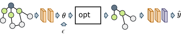
Figure 1: Workflow of the proposed approach.

For every binary adjacency matrix $\bm{Z}\in\mathcal{A}$, we write $\bm{Z}\in\mathcal{F}$ if and only if the adjacency matrix is a feasible solution (not necessarily an optimal one) of the chosen optimization problem. We can now define a discrete exponential family distribution as

$$p(\bm{Z};\bm{\theta})=\left\{\begin{array}[]{ll}\exp\left(\langle\bm{Z},\bm{\theta}\rangle_{F}-B(\bm{\theta})\right)&\text{if }\bm{Z}\in\mathcal{F},\\ 0&\text{otherwise.}\end{array}\right.$$ (3)

where $\langle\cdot,\cdot\rangle_{F}$ is the Frobenius inner product and $B(\bm{\theta})$ is the log-partition function defined as

$$B(\bm{\theta})=\log\left(\sum_{\bm{A}\in\mathcal{F}}\exp\left(\langle\bm{Z},\bm{\theta}\rangle_{F}\right)\right).$$

Hence, $p$ is a probability distribution over adjacency matrices that are feasible solutions to the optimization problem under consideration. Each feasible adjacency matrix’s probability mass is proportional to the product of its edge weights. For example, if the optimization problem is the maximum-weight $k$-edge connected subgraph problem, the distribution assigns a non-zero probability mass to all adjacency matrices of graphs that have $k$ edges and are connected.

Given an optimization problem, we would like to sample exactly from the above probability distribution $p(\bm{Z};\bm{\theta})$. Unfortunately, this is intractable since computing the log-partition function is in general NP-hard. However, as in prior work [Niepert et al., 2021], we can use perturb-and-MAP [Papandreou and Yuille, 2011] to approximately sample from the above distribution as follows. Let $\bm{\epsilon}\sim\rho(\bm{\epsilon})$ be a $n\times n$ matrix of appropriate random variables such as those following the Gumbel distribution. We can then approximately sample an adjacency matrix $\bm{Z}$ from $p(\bm{Z};\bm{\theta})$ by computing

$$\bm{Z}=\mathtt{opt}(\bm{\theta}+\bm{\epsilon}).$$

Hence, we can approximately sample by perturbing the edge weights (unnormalized probabilities) $\bm{\theta}$ and by applying the optimization algorithm to these perturbed weights.

In the final part of the model (the downstream model) we use the sampled $\bm{Z}$ as the input adjacency matrix to a message-passing neural network $f_{\bm{u}}:\mathcal{A}\times\mathcal{X}\rightarrow\mathcal{Y}$ computing $\hat{\bm{y}}=f_{\bm{u}}(\bm{Z},\bm{X})$.

In summary, we have the following model architecture for training input data $(\bm{A},\bm{X},\bm{y})$:

$$\bm{\theta} =h_{\bm{v}}(\bm{A},\bm{X}) \mbox{ with }\ \bm{A}\in\mathcal{A},\bm{X}\in\mathcal{X},$$ (4)

$$\bm{Z} =\mathtt{opt}(\bm{\theta}+\bm{\epsilon}) \mbox{ with }\ \bm{\epsilon}\sim\rho(\epsilon),\bm{\epsilon}\in\mathbb{R}^{n\times n},$$ (5)

$$\hat{\bm{y}} =f_{\bm{u}}(\bm{Z},\bm{X}) \mbox{ with }\ \hat{\bm{y}}\in\mathcal{Y},f_{\bm{u}}:\mathcal{A}\times\mathcal{X}\rightarrow\mathcal{Y}.$$ (6)

Figure 1 illustrates the architecture. With $\bm{\omega}=(\bm{u},\bm{v})$ the learnable parameters of the model and the target variable $\bm{y}$ the loss is now defined as:

$$L(\bm{A},\bm{X},\bm{y};\bm{\omega})=\mathbb{E}_{\bm{\epsilon}\sim\rho(\epsilon)}[\ell(f_{\bm{u}}(\bm{Z},\bm{X}),\bm{y})],$$ (7)

with $\bm{Z}=\mathtt{opt}(\bm{\theta}+\bm{\epsilon})$, $\bm{\theta}=h_{\bm{v}}(\bm{A},\bm{X})$, and $\ell:\mathcal{Y}\times\mathcal{Y}\rightarrow\mathbb{R}^{+}$ a point-wise loss function. The gradient of $L$ wrt $\bm{u}$ is

$$\nabla_{\bm{u}}L(\bm{A},\bm{X},\bm{y};\bm{\omega})=\mathbb{E}[\partial_{\bm{u}}f_{\bm{u}}(\bm{Z},\bm{X})^{\intercal}\nabla_{\bm{y}}\ell(\hat{\bm{y}},\bm{y})]$$

which can be estimated by Monte-Carlo sampling. In contrast, the gradient of $L$ with respect to $\bm{v}$ is:

$$\nabla_{\bm{v}}L(\bm{A},\bm{X},\bm{y};\bm{\omega})=\partial_{\bm{v}}h_{\bm{v}}(\bm{A},\bm{X})^{\intercal}\nabla_{\bm{\theta}}L(\bm{A},\bm{X},\bm{y};\bm{\omega}),$$

where the challenge is to estimate $\nabla_{\bm{\theta}}L(\bm{A},\bm{X},\bm{y};\bm{\omega})=\nabla_{\bm{\theta}}\mathbb{E}_{\bm{\epsilon}\sim\rho(\epsilon)}[\ell(f_{\bm{u}}(\bm{Z},\bm{X}),\bm{y})]$ because $\bm{Z}=\mathtt{opt}(\bm{\theta}+\bm{\epsilon})$ is not continuously differentiable wrt $\bm{\theta}$. While it would be possible to use the score function estimator, its high variance makes it less competitive in practice [Niepert et al., 2021].

4.2 Implicit Maximum-Likelihood Learning

The variant of I-MLE we use in this work estimates $\nabla_{\bm{\theta}}L(\bm{A},\bm{X},\bm{y};\bm{\omega})$ by implicitly creating a target distribution $q(\bm{Z};\bm{\theta}^{\prime})$ using perturbation-based implicit differentiation [Domke, 2010]. Here, the parameters $\bm{\theta}$ are moved in the direction of $-\nabla_{\bm{Z}}\ell(f_{\bm{u}}(\bm{A},\bm{X}),\bm{y}))$, the negative gradient of the downstream loss with respect to the sampled adjacency matrix $\bm{Z}$, to construct $\bm{\theta}^{\prime}$

$$q(\bm{Z};\bm{\theta}^{\prime}):=p(\bm{Z};\bm{\theta}-\lambda\nabla_{\bm{Z}}\ell(f_{\bm{u}}(\bm{Z},\bm{X}),\bm{y}))$$ (8)

with $\bm{Z}=\mathtt{opt}(\bm{\theta}+\bm{\epsilon})$ and $\lambda>0$ the strength of the perturbation. Intuitively, by moving the weights $\bm{\theta}$ into the direction of the negative gradients of $\bm{Z}$, the resulting distribution $q$ is more likely to generate samples with a lower downstream loss. We approximate $\nabla_{\bm{\theta}}L(\bm{A},\bm{X},\bm{y};\bm{\omega})$ with Monte Carlo estimates of the gradients of the KL divergence between $p$ and $q$:

$$\nabla_{\bm{\theta}}L(\bm{A},\bm{X},\bm{y};\bm{\omega})\approx\frac{1}{\lambda}\left(\mathtt{opt}(\bm{\theta}+\bm{\epsilon})-\mathtt{opt}(\bm{\theta}^{\prime}+\bm{\epsilon})\right).$$ (9)

In other words, $\nabla_{\bm{\theta}}L(\bm{A},\bm{X},\bm{y};\bm{\omega})$ is approximated by the difference between an approximate sample from $p(\bm{Z};\bm{\theta})$ and an approximate sample from $q(\bm{Z};\bm{\theta}^{\prime})$. In this way we move the distribution $p(\bm{Z};\bm{\theta})$ closer to $q(\bm{Z};\bm{\theta}^{\prime})$.

Algorithm 1 Greedy algorithm $\mathtt{opt}_{\mathtt{con}}$ for the maximum-weight $k$-edge connected subgraph problem.

Input:

      Input graph $\mathcal{G}=(V,E)$ Number of edges $k$ Edge weights $\bm{\theta}$

Initialize:

      $e=\operatorname*{arg\,max}_{e_{i,j}}\bm{\theta}_{i,j}$ Set of selected edges $S=\{e\}$ Set of edges adjacent to selected edge $N=\mathcal{N}(e)$

while $|S|<k$ and $|N|>0$ do

     $e=\operatorname*{arg\,max}_{e_{i,j}\in N}\bm{\theta}_{i,j}$

     $S=S\cup\{e\}$

     $N=N\cup\mathcal{N}(e)$

     $N=N-S$

end while

Return: Adjacency matrix $\bm{Z}$ of the subgraph induced by the set of selected edges $S$.

4.3 L2xGnn: Learning to Explain GNNs with I-MLE

We now describe the class of L2xGnn models we use in the experiments. First, we need to define the function $h_{\bm{v}}(\bm{A},\bm{X})$. Here we use a standard GNN (see equation 1) to compute for every node $i$ and every layer $\ell$ the vector representation $\mathbf{h}_{i}^{\ell}=h_{\bm{v}}(\bm{A},\bm{X})_{i,1:d}$. We then compute the matrix of edge weights by taking the inner product between each pair of node embeddings. More formally, we compute $\bm{\theta}_{i,j}=\langle\mathbf{h}^{\ell}_{i},\mathbf{h}_{j}^{\ell}\rangle$ for some fixed $\ell$. Typically, we choose $\ell=1$.

In this work, we sample the noise perturbations $\bm{\epsilon}$ from the sum of Gamma distribution [Niepert et al., 2021]. Other noise distributions such as the Gumbel distribution are possible.

4.3.1 Sampling Constrained Subgraphs

An advantage of the proposed method is its ability to integrate any graph optimization problem as long as there exists an algorithm $\mathtt{opt}$ for computing (approximate) solutions. In this work, we focus on two optimization problems: (1) The maximum-weight $k$-edge subgraph and (2) the maximum-weight $k$-edge connected subgraph problems. The former aims to find a maximum-weight subgraph with $k$ edges. The latter aims to find a connected maximum-weight subgraph with $k$ edges. Other optimization problems are possible but we found that sparse and connected subgraphs provide a good efficiency-effectiveness trade-off.

Computing maximum weight $k$-edge subgraphs is highly efficient as we only need to select the $k$ edges with the maximum weights. In order to compute connected $k$-edge subgraphs we use a greedy approach. First, given a number $k$ of edges, we select a single edge $e_{i,j}$ with the highest weight $\bm{\theta}_{i,j}$ from the input graph. At every iteration of the algorithm, we select the next edge such that it (a) is connected to a previously selected edge and (b) has the maximum weight among all those connected edges. A more detailed description of the greedy algorithm is given in Algorithm 1.

Finally, we need to define the function $f_{\bm{u}}$ (the downstream function) of the proposed framework. Here, we again use a message-passing GNN that follows the update rule

$$\mathbf{h}_{i}^{\ell}=\gamma\left(\mathbf{h}_{i}^{\ell-1},\square_{j\in\mathcal{N}(v_{i})}\phi\left(\mathbf{h}_{i}^{\ell-1},\mathbf{h}_{j}^{\ell-1},r_{ij}\right)\right).$$ (10)

The neighborhood structure $\mathcal{N}(\cdot)$, however, is defined through the output adjacency matrix $\bm{Z}$ of the optimization algorithm $\mathtt{opt}$

$$j\in\mathcal{N}(v_{i})\Longleftrightarrow\bm{Z}_{i,j}=\bm{Z}_{j,i}=1.$$ (11)

Hence, if after the subgraph sampling, there exists a node $v_{i}$ which is an isolated node in the adjacency matrix $\bm{Z}$, that is, $\bm{Z}_{i,j}=\bm{Z}_{j,i}=0\ \forall j\in\{1,...,n\}$, the embedding of the node will not be updated based on message passing steps with neighboring nodes. This means that, for isolated nodes, the only information used in the downstream model is the one from the nodes themselves. Conceptually, $\bm{Z}$ works as a mask over the messages $m_{ij}^{\ell}$ computed at each layer $\ell$.

The adjacency matrix $\bm{Z}$ is then used in all subsequent layers of the GNN. In particular, for one layer $\ell$ we have

$$\mathbf{H}_{\ell}=\textsc{Gnn}_{\ell}(\bm{A}\odot\bm{Z},\mathbf{H}_{\ell-1}),$$ (12)

where $\odot$ is the Hadamard product. Finally, the remaining part of the L2xGnn network for the graph classification is

$$\mathbf{h}_{G}=\text{Pool}(\mathbf{H}_{\ell})\qquad\hat{\bm{y}}=\eta(\mathbf{h}_{G}),$$ (13)

where we use a global pooling operator to generate the (sub)graph representation $\mathbf{h}_{G}$ that will then be used by the MLP network $\eta(\cdot)$ to output a probability distribution $\hat{\bm{y}}$ over the class labels. Finally, a loss function is applied whose gradients are used to perform backpropagation. At test time, we use the maximum-probability subgraph for the explanation and prediction, that is, we do not perturb at test time.

5 Experiments

First, we evaluate the predictive performance of the model compared to baselines. Second, we qualitatively and quantitatively analyze the explanatory subgraphs for datasets for which we know the ground-truth motifs. Finally, we analyze whether the generated output can be helpful for model debugging purposes. We report several ablation studies to investigate the effects of different model choices on the results in the supplementary material. The code for reproducing our experiments is available at https://github.com/GiuseppeSerra93/L2XGNN.

5.1 Datasets and Settings

Datasets.

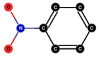
Figure 2: Benzene-NO₂ motif.

To understand the change in the predictive capabilities of the base models when integrating L2xGnn, we use six real-world datasets for graph classification tasks: MUTAG [Debnath et al., 1991], PROTEINS [Borgwardt et al., 2005], YEAST [Yan et al., 2008], IMBD-BINARY, IMBD-MULTI [Yanardag and Vishwanathan, 2015], and DD [Rossi and Ahmed, 2015]. To quantitatively evaluate the quality of the explanations, we use datasets that include ground-truth edge masks. In particular, we use MUTAG₀ and BA2Motifs. MUTAG₀ is a dataset introduced in Tan et al. [2022] which contains the benzene-NO₂ (i.e., a carbon ring with a nitro group (NO₂) attached) as the only discriminative motif between positive and negative labels. A graphical representation of the benzene-NO₂ compound is given in Figure 2. BA2Motifs is a synthetic dataset that was first introduced in Luo et al. [2020]. The base graphs are Barabasi-Albert (BA) graphs. 50% of the graphs are augmented with a house-motif graphs, the rest with a 5-node cycle motif. The discriminative subgraph leading to different predictions is the motif attached to the BA graph.

Experimental settings.

To evaluate the quality of our approach, we use L2xGnn with several GNN base models including GCN [Kipf and Welling, 2017], GIN [Xu et al., 2018] and GraphSAGE [Hamilton et al., 2017]. We compare the results when using the original model and when the same model is combined with our XAI method. For model selection and evaluation, to fairly compare the methods, we follow a previously proposed protocol. The hyperparameter selection is performed via 10-fold cross-validation, where a training fold is randomly used as a validation set. The selection is performed for the number of layers $[1,2,3,4]$ and the number of hidden units $[16,32,64,128]$ based on the validation accuracy. For a fair comparison with the backbone architectures, we select the best configuration for each dataset, and we integrate our approach into the best model. Instead of fixing a value $k$ for each input graph, we compute $k$ based on a ratio $R$ of edges to be kept. Once the hyperparameters of the default model are found, we select the best ratio $R$ from the set of values $[0.4,0.5,0.6,0.7]$ based on the validation accuracy. We do not include extreme values for two reasons: (1) smaller values for $R$ lead to reduced predictive capabilities and do not lead to meaningful explanatory subgraphs; and (2) higher values would not remove enough edges compared to the original input. Finally, we choose the perturbation intensity $\lambda$ from the values $[10,100,1000]$. A summary of the selected hyperparameter values for each configuration can be found in the appendix.

5.2 Empirical Results

Graph Classification Comparison with Base GNNs.

Following the experimental procedure proposed in Zhang et al. [2021], Table 1 lists the results of using L2xGnn with base GNN architectures for graph classification tasks. The primary goal of this work is not to provide a better predictive model, but to provide faithful explanation masks while maintaining similar predictive performance. This analysis is important since inherent interpretable networks are known for creating a trade-off with the predictive capabilities of the model, and practitioners may not be willing to sacrifice the prediction accuracy for increased transparency [Miao et al., 2022]. Nevertheless, we observe that L2xGnn is competitive and often even outperforms the base GNN models on the benchmark datasets.

Table 1: Prediction test accuracy (%) for graph classification tasks over ten runs.

Dataset	GCN			GIN			GraphSAGE
	Original	L2xGnn ${}_{\texttt{dsc}}$	L2xGnn	Original	L2xGnn ${}_{\texttt{dsc}}$	L2xGnn	Original	L2xGnn ${}_{\texttt{dsc}}$	L2xGnn
DD	72.0 $\pm$ 2.4	71.9 $\pm$ 3.1	71.9 $\pm$ 3.6	72.2 $\pm$ 2.7	73.9 $\pm$ 5.1	72.0 $\pm$ 3.0	72.1 $\pm$ 3.9	72.7 $\pm$ 3.8	72.5 $\pm$ 3.9
MUTAG	73.4 $\pm$ 8.3	73.9 $\pm$ 11.1	74.5 $\pm$ 8.2	82.7 $\pm$ 5.1	81.4 $\pm$ 9.2	82.5 $\pm$ 7.8	73.4 $\pm$ 7.5	75.1 $\pm$ 7.7	79.8 $\pm$ 8.1
IMDB-B	73.1 $\pm$ 3.2	66.0 $\pm$ 5.4	73.4 $\pm$ 4.7	72.1 $\pm$ 5.0	65.0 $\pm$ 5.0	72.4 $\pm$ 4.5	72.2 $\pm$ 4.8	73.8 $\pm$ 2.8	73.0 $\pm$ 4.1
IMDB-M	50.0 $\pm$ 2.8	50.3 $\pm$ 3.2	49.0 $\pm$ 2.2	49.0 $\pm$ 4.7	48.8 $\pm$ 3.2	47.9 $\pm$ 3.5	50.7 $\pm$ 3.7	50.6 $\pm$ 3.2	50.8 $\pm$ 2.7
PROTEINS	71.8 $\pm$ 4.4	71.1 $\pm$ 3.4	72.0 $\pm$ 5.3	70.8 $\pm$ 4.5	68.5 $\pm$ 2.9	70.9 $\pm$ 3.4	71.3 $\pm$ 5.1	71.3 $\pm$ 4.1	70.7 $\pm$ 4.6
YEAST	88.1 $\pm$ 0.1	88.2 $\pm$ 0.2	88.1 $\pm$ 0.1	88.3 $\pm$ 0.1	88.2 $\pm$ 0.1	88.0 $\pm$ 0.2	88.2 $\pm$ 0.1	88.0 $\pm$ 0.1	88.1 $\pm$ 0.2

Explanation Accuracy.

We compare the proposed method with popular post-hoc explanation techniques including the GNN-Explainer [Ying et al., 2019], PGE-Explainer [Luo et al., 2020], GradCAM [Pope et al., 2019], GNN-LRP [Schnake et al., 2020], and SubgraphX [Yuan et al., 2021]. We train a 3-layer GIN for $200$ epochs with hidden dimensions equal to $64$ and a learning rate equal to $0.001$. We save the best model according to the validation accuracy and we compare it with the post-hoc techniques. In our case, we integrate L2xGnn into the same architecture and learn the edge masking during training as described before. We report the graph classification results for the two datasets in the appendix. In Table 2, we report the explanation accuracy evaluation with respect to the ground-truth motifs in comparison with post-hoc techniques for 5 different data splits. The explanation problem is formalized as a binary classification problem, where the edges belonging to the ground-truth motif are treated as positive labels. We observe that L2xGnn obtains better or the same results as the considered explanatory models. While for the post-hoc explanation techniques we cannot guarantee that the GNNs use exclusively the explanation subgraphs for the prediction [Yuan et al., 2020b], our method, by providing faithful explanations, overcomes this limitation. It is exactly the provided explanation that is used in the message-passing operations of L2xGnn.

Table 2: Evaluation of explanation accuracy (%) on synthetic graph classification datasets using a 3-layer GIN architecture. The lowest standard deviation for each metric is underlined. With the exception of our proposed method L2xGnn, none of the approaches can guarantee faithful explanations where the explanation is exclusively used during message passing operations.

Dataset	BA-2MOTIFS				MUTAG0
	Acc.	Pr.	Rec.	F1	Acc.	Pr.	Rec.	F1
GNN-Exp.	44.6 $\pm$ 2.4	22.7 $\pm$ 0.9	62.9 $\pm$ 3.3	32.9 $\pm$ 1.0	47.4 $\pm$ 2.3	42.2 $\pm$ 2.4	69.2 $\pm$ 2.4	50.2 $\pm$ 2.1
GradCAM	77.1 $\pm$ 11.5	50.1 $\pm$ 16.1	72.4 $\pm$ 23.2	59.0 $\pm$ 19.0	78.0 $\pm$ 1.3	85.6 $\pm$ 2.8	60.8 $\pm$ 3.9	68.8 $\pm$ 2.2
PGE-Exp.	36.7 $\pm$ 18.9	17.5 $\pm$ 5.9	66.6 $\pm$ 22.5	27.7 $\pm$ 9.4	65.0 $\pm$ 9.6	57.3 $\pm$ 12.3	54.7 $\pm$ 12.2	54.9 $\pm$ 12.0
GNN-LRP	77.3 $\pm$ 2.5	34.3 $\pm$ 16.8	36.4 $\pm$ 19.7	33.0 $\pm$ 15.7	71.7 $\pm$ 7.3	78.6 $\pm$ 9.2	43.5 $\pm$ 16.7	53.4 $\pm$ 17.1
SubgraphX	81.5 $\pm$ 5.6	54.0 $\pm$ 12.9	74.2 $\pm$ 16.5	60.4 $\pm$ 14.2	72.2 $\pm$ 2.1	76.1 $\pm$ 2.8	47.6 $\pm$ 5.9	56.8 $\pm$ 3.3
L2xGnn	78.0 $\pm$ 0.6	49.5 $\pm$ 0.8	90.2 $\pm$ 1.4	63.8 $\pm$ 1.0	74.1 $\pm$ 4.3	65.6 $\pm$ 3.9	82.8 $\pm$ 5.2	70.7 $\pm$ 4.3
L2xGnn ${}_{\texttt{dsc}}$	80.0 $\pm$ 1.2	52.1 $\pm$ 1.6	94.7 $\pm$ 2.7	67.1 $\pm$ 2.0	71.0 $\pm$ 3.0	62.4 $\pm$ 4.1	78.1 $\pm$ 3.2	66.9 $\pm$ 3.5

Qualitative Evaluation of the Explanations.

In Figure 5, we present some of the subgraphs identified by L2xGnn when combined with two different base GNNs. Based on prior studies and chemical domain knowledge [Debnath et al., 1991, Lin et al., 2021, Tan et al., 2022], carbon rings (the black circles in the pictures) and $\text{NO}_{2}$ groups are known to be mutagenic. Interestingly, we can notice that, when using the information of connected subgraphs, the models are able to recognize a complete carbon ring with a $\text{NO}_{2}$ group in most of the cases. In some cases, the carbon ring is not complete, but the explanations are still helpful to understand which motifs are potentially important for the prediction. In the second row, we can observe the results of the sampling strategy where we do not require subgraphs to be connected. In this case, the carbon rings are not always identified. Instead, the $\text{NO}_{2}$ group is always considered important for the prediction. More generally, as also reported in Yuan et al. [2021], studying connected subgraphs results in more natural motifs compared to the motifs obtained without the connectedness constraint. The visualization of explanations for GraphSAGE and other methods can be found in the supplementary material.

	GCN		GIN
$w/$ ${con}$
$w/o$ ${con}$

Figure 3: Visualization of some of the subgraphs selected by L2xGnn for MUTAG₀ on the test set. The solid edges are the ones sampled by our approach. The first and second rows depict, respectively, some motifs with or without constraining the subgraphs to be connected. Black, blue, red, and gray nodes represent carbon (C), nitrogen (N), oxygen (O), and hydrogen (H) atoms respectively.

GCN		GIN

Figure 4: Example of model reasoning understanding through the visualization of the generated explanations.

Shortcut Learning Detection.

By generating faithful subgraph explanations, our approach can be used to detect whether the predictive model is focusing on the expected features or if it is affected by shortcut learning. This is particularly important for GNNs, where seemingly small implementation differences can influence the learning process of the model [Schlichtkrull et al., 2021]. To this end, we use the BA2Motifs dataset [Luo et al., 2020]. We trained two different models, GCN and GIN, achieving a test accuracy of $0.67$ and $1.0$ respectively. Taking a closer look at the explanations of the first model, we observed that most of the correct predictions were (incorrectly) correlated with the cycle motif and that the explanations were similar to the ones reported in Figure 4. The explanatory results show that the model is not learning the expected discriminative motifs and, consequently, the accuracy for the test set is poor. This insight can help users to change the configuration of the architecture or to use a different model (e.g., GIN). More generally, the results highlight that faithful explanations can facilitate model analysis and debugging.

6 Conclusion and Limitations

We propose L2xGnn, a framework that can be integrated into GNN architectures to learn to generate explanatory subgraphs which are exclusively used for the models’ predictions. Our experimental findings demonstrate that the integration of L2xGnn with base GNNs does not affect the predictive capabilities of the model for graph classification tasks. Furthermore, according to the definition provided in the paper, the resulting explanations are faithful since the retained information is the only one used by the model for prediction. Hence, differently from most of the common techniques, our explanations reveal the rationale of the GNNs and can also be used for model analysis and debugging.

A limitation of the approach is the reduced efficiency compared to baseline GNN models. Since we need to integrate an algorithm to compute (approximate) solutions to a combinatorial optimization problem, each forward-pass requires more time and resources. Moreover, depending on the choice of the optimization problem, we might not capture the structure of explanatory motifs required for the application under consideration.

A Dataset Statistics

In Table 3, we report the statistics of the datasets used for graph classification tasks. We use datasets from different domains including biological data, social networks, and bioinformatics data. For a comprehensive evaluation, we include datasets with different characteristics, such as a larger number of graphs or a larger number of nodes and edges.

Table 3: Statistics of the datasets.

Number of	Nodes (avg)	Edges (avg)	Graphs	Classes
DD	284.32	715.66	1178	2
MUTAG	17.93	19.79	188	2
IMDB-B	19.77	96.53	1000	2
IMDB-M	13.00	65.94	1500	3
PROTEINS	39.06	72.82	1113	2
YEAST	21.54	22.84	79601	2

B Hyperparameter Selection

Experiments were run on a single Linux machine with Intel Core i7-11370H @ 3.30GHz, 1 GeForce RTX 3060, and 16 GB RAM. The best hyperparameter configuration for each model and dataset used for graph classification tasks is reported in Table 4. The selection is performed via 10-fold cross-validation according to the validation accuracy. First, for the backbone architectures, we consider the number of layers $[1,2,3,4]$ and the number of hidden units $[16,32,64,128]$. Then, for L2xGnn, we select the ratio $R$ from $[0.4,0.5,0.6,0.7]$ and the perturbation intensity $\lambda$ from $[10,100,1000]$.

Table 4: Hyperparameter settings for graph classification tasks.

Dataset	GCN				GIN				GraphSAGE
	Hidden	Layers	$R$	$\lambda$	Hidden	Layers	$R$	$\lambda$	Hidden	Layers	$R$	$\lambda$
DD	128	2	0.6	10	64	1	0.5	100	128	1	0.6	100
MUTAG	128	3	0.6	1000	128	4	0.5	10	128	3	0.4	10
IMDB-B	128	3	0.4	100	64	3	0.4	1000	64	1	0.4	10
IMDB-M	64	3	0.6	10	128	4	0.6	10	64	1	0.4	100
PROTEINS	128	3	0.7	100	128	4	0.5	10	64	3	0.4	10
YEAST	128	3	0.6	10	128	3	0.6	10	32	4	0.5	100

C Comparison with Non-post-hoc Methods

Among the plethora of post-hoc methods for graphs, ProtGNN [Zhang et al., 2021] and KerGNN [Feng et al., 2022a] are noteworthy exceptions. The first approach proposes a framework to generate explanations by comparing input graphs with prototypes learned during training, The latter, instead, combines graph kernels with the message passing paradigm to learn hidden graph filters. In contrast to these methods, our approach only relies on standard GNNs, without the use of prototypes or graph kernels. Consequently, even though both ProtGNN and KerGNN provide built-in explanations, they are not faithful by design as they introduce a new mechanism to compute graph representations which differs from standard GNNs computations. In terms of explanatory capability, the learned prototypes are not directly interpretable and need to be matched to the closest training subgraphs to be human-understandable. Graph filters, instead, do not necessarily match existing patterns in the instance-based case. In both cases, the output can only provide a general idea of the important structures used by the model for prediction but fail at revealing precisely the instance-level explanation for each input graph. For these reasons, a direct comparison with the two methods is not possible.

D Comparison with Graph Structure Learning Approaches

Recently, there have been related methods for learning the structure of graph neural networks. Following the taxonomy proposed in Zhu et al. [2021], the structure learning methods most related to L2xGnn fall into the postprocessing category, and more specifically, under the discrete sampling subcategory. All existing methods use variants of the Gumbel-softmax trick which is limited in modeling complex distributions. Moreover, only when the straight-through version of the Gumbel-softmax trick is used, one can obtain truly discrete and not merely relaxed adjacency matrices in the forward pass. In contrast, L2xGnn always samples purely discrete adjacency matrices. It is, to the best of our knowledge, the only method that allows us to model complex dependencies between the edge variables through its ability to integrate a combinatorial optimization algorithm on graphs. Other strategies include sampling edges between each pair of nodes from a Bernoulli distribution [Franceschi et al., 2019] or sampling subgraphs for subgraph aggregation methods in a data-driven manner [Qian et al., 2022]. All these methods, however, are not concerned with the problem of explaining the behavior of GNNs explicitly.

Table 5: Effect of the edge ratio on the prediction accuracy (%).

Ratio	0.2	0.3	0.4	0.5	0.6	0.7	0.8	0.9
	MUTAG
GCN	72.4 $\pm$ 9.4	73.5 $\pm$ 11.4	72.9 $\pm$ 7.6	73.8 $\pm$ 7.2	71.3 $\pm$ 7.3	70.8 $\pm$ 8.6	75.5 $\pm$ 10.6	70.8 $\pm$ 11.1
GIN	78.2 $\pm$ 8.6	79.8 $\pm$ 8.2	82.8 $\pm$ 3.8	84.6 $\pm$ 8.3	80.9 $\pm$ 8.2	76.0 $\pm$ 11.2	77.6 $\pm$ 10.9	80.3 $\pm$ 9.3
	PROTEINS
GCN	71.9 $\pm$ 3.0	71.6 $\pm$ 3.9	72.3 $\pm$ 4.5	72.4 $\pm$ 3.7	72.9 $\pm$ 3.1	72.4 $\pm$ 4.8	72.1 $\pm$ 4.5	72.6 $\pm$ 4.6
GIN	68.3 $\pm$ 2.2	69.2 $\pm$ 3.8	69.7 $\pm$ 2.3	70.5 $\pm$ 4.5	70.1 $\pm$ 5.6	69.7 $\pm$ 5.7	70.4 $\pm$ 4.4	70.9 $\pm$ 4.3

E Ablation Study

In the graph classification task, we compare the two sampling strategies. From the results, the connected sampling is able to get better results than the non-connected counterpart on most datasets. In fact, the connectivity of subgraphs is essential to grasp the complete information about the important patterns, especially for chemical compound data where connected atoms are usually expected to create molecules or chemical groups. This aspect is also supported by the results obtained in the explanation accuracy task, where the connected strategy returns better explanations for the chemical dataset. Additionally, as previously mentioned, evaluating connected structures rather than just important edges looks more natural and intelligible. In Table 5, we analyze the effect of the quantity of retained information on the prediction accuracy. A smaller ratio indicates that we retain fewer edges during training and, consequently, the resulting subgraphs are more sparse and, therefore, interpretable. As one can see, this affects the predictive capabilities only when $R$ is small. Starting from $R=0.5$, the ratio does not affect particularly the predictive capabilities of the model. In fact, for graph classification tasks, some of the information contained in the initial computational graph does not condition the prediction as the information may be redundant or noisy. For instance, considering the MUTAG dataset, we know that the initial graphs contain on average 20 edges. The discriminative motif benzene-$\text{NO}_{2}$, instead, contains around 9 edges, meaning that we ideally need 50% of the original edges to obtain good results. This is in line with the findings of this analysis and the graph classification results previously reported in the main paper.

F Time Complexity Analysis

As reported in Feng et al. [2022a], most message-passing architectures have a time complexity of $\mathcal{O}(n^{2})$. Thus, since L2xGnn uses native GNNs, it also has a worst-case complexity of $\mathcal{O}(n^{2})$. KerGNN instead, being based on graph kernels, has a time complexity between $\mathcal{O}(n^{2})$ and $\mathcal{O}(n^{3})$ in case the graph is fully-connected. The time overhead of $\mathtt{opt}$ depends on the algorithm used. For the maximum-weight $k$-edge subgraph problem, we only need to select the $k$ edges with the maximum weights. To find the maximum-weight $k$-edge connected subgraph, the greedy algorithm needs to find the maximum weight edge among all edges adjacent to the currently selected subgraph which, in the worst case, are all edges.
Finally, to conclude the comparison with post-hoc techniques, we analyze the time efficiency for generating explanations for unseen data. For a coherent comparison, we use the same test splits used for the previous experiments. Table 6 reports the average time cost to obtain the explanations related to the graphs in the test sets.

Table 6: Evaluation of the average execution time (in sec) for generating explanations of unseen data.

Dataset	BA-2MOTIFS (size = 100)		MUTAG0 (size = 223)
	Nodes (avg)	Edges (avg)	Nodes (avg)	Edges (avg)
	25.0	51.0	31.74	32.54
GNN-Exp.	227.10 $\pm$ 1.18		529.43 $\pm$ 2.02
GradCAM	1.41 $\pm$ 0.17		2.66 $\pm$ 0.03
PGE-Exp.	0.64 $\pm$ 0.02		1.74 $\pm$ 0.25
GNN-LRP	918.42 $\pm$ 32.26		1938.98 $\pm$ 38.14
SubgraphX	3500.66 $\pm$ 358.31		25585.26 $\pm$ 1143.18
L2xGnn ${}_{\texttt{dsc}}$	0.74 $\pm$ 0.04		0.61 $\pm$ 0.01
L2xGnn	0.73 $\pm$ 0.02		1.08 $\pm$ 0.02

G Graph Classification Accuracy for Synthetic Datasets

In Table 7, we report the graph classification accuracy for the datasets used in our explanation accuracy experiment. In particular, we compare the 3-layer GIN architecture used for generating explanations through post-hoc techniques and the same architecture when our approach is integrated during training. The data splits are the same used in the previous evaluation. Again, the results demonstrate that the integration of L2xGnn does not degrade significantly the predictive capabilities of the original model.

Table 7: Comparison of the prediction test accuracy (%) for synthetic graph classification tasks between a 3-layer GIN architecture and the same architecture with our approach integrated.

Dataset	BA-2MOTIFS	MUTAG0
GIN	100.0 $\pm$ 0.00	100.0 $\pm$ 0.00
L2xGnn ${}_{\texttt{dsc}}$	99.6 $\pm$ 0.04	99.9 $\pm$ 0.01
L2xGnn	99.6 $\pm$ 0.04	99.6 $\pm$ 0.03

H Visual Comparison of Generated Explanations

In Figure 5 we provide a visual analysis of the explanations generated by the methods considered in our experiments. The graph visualization supports the numerical evaluation carried on in the main paper. In fact, one can see that the explanations generated by the post-hoc approaches may vary substantially depending on the given input graph. In our case, instead, the explanations remain constant regardless of the input information. This claim supports the explanation accuracy analysis, where our approach has one of the smallest standard deviation among all the considered methods. Additionally, we also included the explanations generated with an attention-based GNN, namely GAT [Veličković et al., 2018]. Although having a similar predictive performance in the graph classification task (99.6 $\pm$ 0.03), the resulting explanations are not qualitatively comparable with our approach. This is in line with previous work [Ying et al., 2019, Yu et al., 2020, Miao et al., 2022] asserting that graph attention models are not able to generate attention weights with high-fidelity, and consequently, cannot provide faithful and meaningful explanations.

GNN-Exp.
GradCAM
PGE-Exp.
GNN-LRP
SubgraphX
GAT
GraphSAGE dsc
GraphSAGE con

Figure 5: Comparison of the generated explanations for MUTAG₀ on the test set. The solid edges are the ones considered responsible of a correct prediction. Black, blue, red, gray, and green nodes represent carbon (C), nitrogen (N), oxygen (O), hydrogen (H), and chlorine (Cl) atoms respectively.

References

- Agarwal et al. [2022a] Chirag Agarwal, Owen Queen, Himabindu Lakkaraju, and Marinka Zitnik. An explainable ai library for benchmarking graph explainers. 2022a.
- Agarwal et al. [2022b] Chirag Agarwal, Marinka Zitnik, and Himabindu Lakkaraju. Probing gnn explainers: A rigorous theoretical and empirical analysis of gnn explanation methods. In International Conference on Artificial Intelligence and Statistics, pages 8969–8996, 2022b.
- Baldassarre and Azizpour [2019] Federico Baldassarre and Hossein Azizpour. Explainability techniques for graph convolutional networks. arXiv preprint arXiv:1905.13686, 2019.
- Borgwardt et al. [2005] Karsten M Borgwardt, Cheng Soon Ong, Stefan Schönauer, SVN Vishwanathan, Alex J Smola, and Hans-Peter Kriegel. Protein function prediction via graph kernels. Bioinformatics, 21(suppl_1):i47–i56, 2005.
- Chen et al. [2018] Jianbo Chen, Le Song, Martin Wainwright, and Michael Jordan. Learning to explain: An information-theoretic perspective on model interpretation. In International Conference on Machine Learning, pages 883–892. PMLR, 2018.
- Debnath et al. [1991] Asim Kumar Debnath, Rosa L Lopez de Compadre, Gargi Debnath, Alan J Shusterman, and Corwin Hansch. Structure-activity relationship of mutagenic aromatic and heteroaromatic nitro compounds. correlation with molecular orbital energies and hydrophobicity. Journal of medicinal chemistry, 34(2):786–797, 1991.
- Domke [2010] Justin Domke. Implicit differentiation by perturbation. Advances in Neural Information Processing Systems, 23:523–531, 2010.
- Duval and Malliaros [2021] Alexandre Duval and Fragkiskos D Malliaros. Graphsvx: Shapley value explanations for graph neural networks. In Joint European Conference on Machine Learning and Knowledge Discovery in Databases, pages 302–318. Springer, 2021.
- Faber et al. [2021] Lukas Faber, Amin K. Moghaddam, and Roger Wattenhofer. When comparing to ground truth is wrong: On evaluating gnn explanation methods. In Proceedings of the 27th ACM SIGKDD Conference on Knowledge Discovery & Data Mining, pages 332–341, 2021.
- Feng et al. [2022a] Aosong Feng, Chenyu You, Shiqiang Wang, and Leandros Tassiulas. Kergnns: Interpretable graph neural networks with graph kernels. arXiv preprint arXiv:2201.00491, 2022a.
- Feng et al. [2022b] Qizhang Feng, Ninghao Liu, Fan Yang, Ruixiang Tang, Mengnan Du, and Xia Hu. DEGREE: Decomposition based explanation for graph neural networks. In International Conference on Learning Representations, 2022b.
- Franceschi et al. [2019] Luca Franceschi, Mathias Niepert, Massimiliano Pontil, and Xiao He. Learning discrete structures for graph neural networks. In International conference on machine learning, pages 1972–1982, 2019.
- Gao et al. [2021] Yuyang Gao, Tong Sun, Rishab Bhatt, Dazhou Yu, Sungsoo Hong, and Liang Zhao. Gnes: Learning to explain graph neural networks. In 2021 IEEE International Conference on Data Mining (ICDM), pages 131–140. IEEE, 2021.
- Gui et al. [2022] Shurui Gui, Hao Yuan, Jie Wang, Qicheng Lao, Kang Li, and Shuiwang Ji. Flowx: Towards explainable graph neural networks via message flows. arXiv preprint arXiv:2206.12987, 2022.
- Hamilton et al. [2017] William L Hamilton, Rex Ying, and Jure Leskovec. Inductive representation learning on large graphs. In Proceedings of the 31st International Conference on Neural Information Processing Systems, pages 1025–1035, 2017.
- Huang et al. [2020] Qiang Huang, Makoto Yamada, Yuan Tian, Dinesh Singh, Dawei Yin, and Yi Chang. Graphlime: Local interpretable model explanations for graph neural networks. arXiv preprint arXiv:2001.06216, 2020.
- Kipf and Welling [2017] Thomas N Kipf and Max Welling. Semi-supervised classification with graph convolutional networks. In International Conference on Learning Representations, 2017.
- Lee et al. [2019] Junhyun Lee, Inyeop Lee, and Jaewoo Kang. Self-attention graph pooling. In International conference on machine learning, pages 3734–3743. PMLR, 2019.
- Lin et al. [2021] Wanyu Lin, Hao Lan, and Baochun Li. Generative causal explanations for graph neural networks. In International Conference on Machine Learning, pages 6666–6679. PMLR, 2021.
- Liu et al. [2021] Meng Liu, Youzhi Luo, Limei Wang, Yaochen Xie, Hao Yuan, Shurui Gui, Haiyang Yu, Zhao Xu, Jingtun Zhang, Yi Liu, Keqiang Yan, Haoran Liu, Cong Fu, Bora M Oztekin, Xuan Zhang, and Shuiwang Ji. DIG: A turnkey library for diving into graph deep learning research. Journal of Machine Learning Research, 22(240):1–9, 2021. URL http://jmlr.org/papers/v22/21-0343.html.
- Lucic et al. [2022] Ana Lucic, Maartje A Ter Hoeve, Gabriele Tolomei, Maarten De Rijke, and Fabrizio Silvestri. Cf-gnnexplainer: Counterfactual explanations for graph neural networks. In International Conference on Artificial Intelligence and Statistics, pages 4499–4511. PMLR, 2022.
- Luo et al. [2020] Dongsheng Luo, Wei Cheng, Dongkuan Xu, Wenchao Yu, Bo Zong, Haifeng Chen, and Xiang Zhang. Parameterized explainer for graph neural network. arXiv preprint arXiv:2011.04573, 2020.
- Magister et al. [2021] Lucie Charlotte Magister, Dmitry Kazhdan, Vikash Singh, and Pietro Liò. Gcexplainer: Human-in-the-loop concept-based explanations for graph neural networks. arXiv preprint arXiv:2107.11889, 2021.
- Miao et al. [2022] Siqi Miao, Mia Liu, and Pan Li. Interpretable and generalizable graph learning via stochastic attention mechanism. In International Conference on Machine Learning, pages 15524–15543. PMLR, 2022.
- Niepert et al. [2021] Mathias Niepert, Pasquale Minervini, and Luca Franceschi. Implicit MLE: backpropagating through discrete exponential family distributions. In NeurIPS, Proceedings of Machine Learning Research. PMLR, 2021.
- Papandreou and Yuille [2011] G. Papandreou and A. L. Yuille. Perturb-and-map random fields: Using discrete optimization to learn and sample from energy models. In 2011 International Conference on Computer Vision, pages 193–200, 2011.
- Perotti et al. [2022] Alan Perotti, Paolo Bajardi, Francesco Bonchi, and André Panisson. Graphshap: Motif-based explanations for black-box graph classifiers. arXiv preprint arXiv:2202.08815, 2022.
- Pope et al. [2019] Phillip E Pope, Soheil Kolouri, Mohammad Rostami, Charles E Martin, and Heiko Hoffmann. Explainability methods for graph convolutional neural networks. In Proceedings of the IEEE/CVF Conference on Computer Vision and Pattern Recognition, pages 10772–10781, 2019.
- Qian et al. [2022] Chendi Qian, Gaurav Rattan, Floris Geerts, Christopher Morris, and Mathias Niepert. Ordered subgraph aggregation networks. arXiv preprint arXiv:2206.11168, 2022.
- Rossi and Ahmed [2015] Ryan Rossi and Nesreen Ahmed. The network data repository with interactive graph analytics and visualization. In Twenty-ninth AAAI conference on artificial intelligence, 2015.
- Rudin [2018] C Rudin. Stop explaining black box machine learning models for high stakes decisions and use interpretable models instead. In Proceedings of NeurIPS 2018 Workshop on Critiquing and Correcting Trends in Learning, 2018.
- Sanchez-Lengeling et al. [2020] Benjamin Sanchez-Lengeling, Jennifer Wei, Brian Lee, Emily Reif, Peter Wang, Wesley Qian, Kevin McCloskey, Lucy Colwell, and Alexander Wiltschko. Evaluating attribution for graph neural networks. Advances in neural information processing systems, 33:5898–5910, 2020.
- Schlichtkrull et al. [2021] Michael Sejr Schlichtkrull, Nicola De Cao, and Ivan Titov. Interpreting graph neural networks for {nlp} with differentiable edge masking. In International Conference on Learning Representations, 2021.
- Schnake et al. [2020] Thomas Schnake, Oliver Eberle, Jonas Lederer, Shinichi Nakajima, Kristof T Schütt, Klaus-Robert Müller, and Grégoire Montavon. Higher-order explanations of graph neural networks via relevant walks. arXiv preprint arXiv:2006.03589, 2020.
- Schwarzenberg et al. [2019] Robert Schwarzenberg, Marc Hübner, David Harbecke, Christoph Alt, and Leonhard Hennig. Layerwise relevance visualization in convolutional text graph classifiers. arXiv preprint arXiv:1909.10911, 2019.
- Tan et al. [2022] Juntao Tan, Shijie Geng, Zuohui Fu, Yingqiang Ge, Shuyuan Xu, Yunqi Li, and Yongfeng Zhang. Learning and evaluating graph neural network explanations based on counterfactual and factual reasoning. In Proceedings of the ACM Web Conference 2022, pages 1018–1027, 2022.
- Veličković et al. [2018] Petar Veličković, Guillem Cucurull, Arantxa Casanova, Adriana Romero, Pietro Liò, and Yoshua Bengio. Graph attention networks. In International Conference on Learning Representations, 2018.
- Vu and Thai [2020] Minh N Vu and My T Thai. Pgm-explainer: Probabilistic graphical model explanations for graph neural networks. arXiv preprint arXiv:2010.05788, 2020.
- Xu et al. [2018] Keyulu Xu, Weihua Hu, Jure Leskovec, and Stefanie Jegelka. How powerful are graph neural networks? In International Conference on Learning Representations, 2018.
- Xuanyuan et al. [2022] Han Xuanyuan, Pietro Barbiero, Dobrik Georgiev, Lucie Charlotte Magister, and Pietro Lió. Global concept-based interpretability for graph neural networks via neuron analysis. arXiv preprint arXiv:2208.10609, 2022.
- Yan et al. [2008] Xifeng Yan, Hong Cheng, Jiawei Han, and Philip S Yu. Mining significant graph patterns by leap search. In Proceedings of the 2008 ACM SIGMOD international conference on Management of data, pages 433–444, 2008.
- Yanardag and Vishwanathan [2015] Pinar Yanardag and SVN Vishwanathan. Deep graph kernels. In Proceedings of the 21th ACM SIGKDD international conference on knowledge discovery and data mining, pages 1365–1374, 2015.
- Ying et al. [2019] Rex Ying, Dylan Bourgeois, Jiaxuan You, Marinka Zitnik, and Jure Leskovec. Gnnexplainer: Generating explanations for graph neural networks. Advances in neural information processing systems, 32:9240, 2019.
- Ying et al. [2018] Zhitao Ying, Jiaxuan You, Christopher Morris, Xiang Ren, Will Hamilton, and Jure Leskovec. Hierarchical graph representation learning with differentiable pooling. Advances in neural information processing systems, 31, 2018.
- Yu et al. [2020] Junchi Yu, Tingyang Xu, Yu Rong, Yatao Bian, Junzhou Huang, and Ran He. Graph information bottleneck for subgraph recognition. In International Conference on Learning Representations, 2020.
- Yu and Gao [2022] Zhaoning Yu and Hongyang Gao. Motifexplainer: a motif-based graph neural network explainer. arXiv preprint arXiv:2202.00519, 2022.
- Yuan et al. [2020a] Hao Yuan, Jiliang Tang, Xia Hu, and Shuiwang Ji. Xgnn: Towards model-level explanations of graph neural networks. In Proceedings of the 26th ACM SIGKDD International Conference on Knowledge Discovery & Data Mining, pages 430–438, 2020a.
- Yuan et al. [2020b] Hao Yuan, Haiyang Yu, Shurui Gui, and Shuiwang Ji. Explainability in graph neural networks: A taxonomic survey. arXiv preprint arXiv:2012.15445, 2020b.
- Yuan et al. [2021] Hao Yuan, Haiyang Yu, Jie Wang, Kang Li, and Shuiwang Ji. On explainability of graph neural networks via subgraph explorations. arXiv preprint arXiv:2102.05152, 2021.
- Zhang et al. [2018] Muhan Zhang, Zhicheng Cui, Marion Neumann, and Yixin Chen. An end-to-end deep learning architecture for graph classification. In Proceedings of the AAAI conference on artificial intelligence, volume 32, 2018.
- Zhang et al. [2021] Zaixi Zhang, Qi Liu, Hao Wang, Chengqiang Lu, and Cheekong Lee. Protgnn: Towards self-explaining graph neural networks. arXiv preprint arXiv:2112.00911, 2021.
- Zhu et al. [2021] Yanqiao Zhu, Weizhi Xu, Jinghao Zhang, Qiang Liu, Shu Wu, and Liang Wang. Deep graph structure learning for robust representations: A survey. arXiv preprint arXiv:2103.03036, 2021.