FIRE: A Failure-Adaptive Reinforcement Learning Framework for Edge Computing Migrations

Abstract

In edge computing, users’ service profiles must be migrated in response to user mobility. Reinforcement learning (RL) frameworks have been proposed to do so. Nevertheless, these frameworks do not consider occasional server failures, which although rare, can prevent the smooth and safe functioning of edge computing users’ latency sensitive applications such as autonomous driving and real-time obstacle detection, because users’ computing jobs can no longer be completed. As these failures occur at a low probability, it is difficult for RL algorithms, which are inherently data-driven, to learn an optimal service migration solution for both the typical and rare event scenarios. Therefore, we introduce a rare events adaptive resilience framework FIRE, which integrates importance sampling into reinforcement learning to place backup services. We sample rare events at a rate proportional to their contribution to the value function, to learn an optimal policy. Our framework balances service migration trade-offs between delay and migration costs, with the costs of failure and the costs of backup placement and migration. We propose an importance sampling based Q-learning algorithm, and prove its boundedness and convergence to optimality. Following which we propose novel eligibility traces, linear function approximation and deep Q-learning versions of our algorithm to ensure it scales to real-world scenarios. We extend our framework to cater to users with different risk tolerances towards failure. Finally, we use trace driven experiments to show that our algorithm gives cost reductions in the event of failures.

I Introduction

Mobile (or multi-access) edge computing (MEC) is a key technology in the fifth-generation (5G) and 6G telecommunication systems. It enables computationally intensive and latency sensitive mobile applications such as real time image processing, augmented reality, mobile big data analytics, interactive gaming, etc. In MEC, computing resources such as a cluster of servers are placed geographically close to end-users, for example at cellular base stations or WiFi access points at the network edge of the radio access network (RAN) [1, 2]. Users can offload their computationally intensive jobs to these resources. Their geographical proximity helps enable latency sensitive applications, by avoiding wide-area network delay experienced when jobs are offloaded to the cloud [3].

Researchers have been actively investigating how to jointly allocate computing and radio resources for end users [1, 4, 5, 6, 7]. Nevertheless, user mobility across geographical areas presents a challenge towards task offloading [8, 9, 10]. As a user moves across coverage areas, keeping its service profile at its original location may lead to higher user-perceived latency, due to the increase in network distance. Therefore, service migration has been proposed as a strategy which consists of migrating the users’ service profiles to MEC nodes nearer the user, to decrease the user-experienced latency [9, 10]. At the same time, constant service migration in response to user movement causes additional expenditure, due to the increase in energy consumption and usage of the wide-area-network (WAN)’s bandwidth. Hence, service migration while balancing the delay-cost tradeoff, under various scenarios, has been a widely studied problem [8, 11, 9, 12, 13, 14, 15].

I-A Challenges: Edge Computing and Resilience

Few migration works, however, account for another challenge in edge computing: the resilience of edge computing systems to rare but serious events like server failures. They occur due to reasons such as system overload, hardware failures, or malicious attacks, and they can be costly: the average cost of outage at a cloud data center, for example, has increased to $\$740000$ in $2016$ [16]. In comparison to the cloud, failures at edge servers are even more likely, as edge servers are distributed across geographical locations, making their management and maintenance more challenging. Furthermore, unlike the cloud, due to their distributed nature, edge servers do not have advanced heat management or outage support systems such as direct liquid cooling, fire suppressing gaseous systems and fully duplicated electrical lines with transfer switches [17]. Even if edge server failures remain fairly rare, they have a sizeable impact as many edge computing applications are latency sensitive, such as the Internet of vehicles, augmented reality, and video processing applications [1]. A lack of adaptive resource allocation and scheduling policies in light of failures would result in an increase in computation delay and a decrease in the job completion probability. For instance, if the user’s service profile is migrated to an access point that then experiences a server failure, its job is not able to be completed, jeopardizing the smooth and safe functioning of applications, such as autonomous driving and real time obstacle detection.

The core question addressed in this work is: How can the network operator make edge computing systems resilient to such failures, and thus ensure smooth and safe application functioning? We propose the use of backups to do so. Backup services, which are placed at a different edge server from the primary service, can take over if the primary service’s edge server fails, allowing the application to continue functioning. Managing the migration of both the primary and backup services, however, is challenging, as the number of potential migration paths grows at least exponentially as the number of access points and timeslots increases. Furthermore, the network operator has a lack of knowledge of the user mobility distributions and the corresponding costs resulting from mobility. Markov decision processes and reinforcement learning has been traditionally proposed as a method to solve the service migration problem [8, 11, 18, 19]. Nevertheless, these rare events and failures occur at a low probability, making it difficult to jointly plan or learn an optimal resource allocation policy for both the usual and rare event scenarios. This is because reinforcement learning relies on past reward data. The low probabilities of rare events may make the learner miss the importance of rare events, impacting the training of the learning algorithm [20]. Therefore, we introduce FIRE: Failure-adaptive Importance sampling for Rare Events, a resilience framework for edge computing service migration.

I-B FIRE: Failure-adaptive Importance sampling for Rare Events

Our framework uses reinforcement learning to optimize service migration and the placement of backups in the edge computing system, in light of potential (but rare) service failures. Besides optimizing for the service profile placements, we optimize the placement of service profile backups across the MEC system, while considering the storage and migration cost they incur. The placement of backups allows users’ jobs to still be computed even if the server in which their profile was placed at fails. Deciding where to place these backups, however, is a difficult problem as they, like the primary service, should move with the user. Because the actual rare event probability is low and unable to help us learn an optimal policy to prepare for rare events, we use importance sampling to increase the sampling of the rare events. We sample at a rate which represents their contribution to system wide costs, to help us prepare for rare events. Error correction is done through the use of importance sampling weights, to enable us to learn an optimal policy with respect to the true rare events probability. To avoid the large failure costs experienced during server failures in online scenarios, training is done in a simulator mode. The converged policy trained by the simulator is then applied to online scenarios, in which rare events happen at their natural probabilities. While the focus of our framework in this paper is for service migration, our importance sampling framework is able to be extended and modified, to tackle other resource allocation and decision making problems in light of rare events in networking and communications.

In edge computing, users may have heterogeneous risk tolerances, due to their differing computing applications, with differing latency requirements. Some users may have a higher risk tolerance for edge server failures due to their application being less latency sensitive than others, or may not be willing to incur a cost of placing backups during normal scenarios to prepare for potential failures. In light of this, we also propose an algorithm that caters to users of different risk tolerances, without requiring separate algorithm training for different risk tolerances.

In summary, the contributions of this paper are as follows:

• We introduce FIRE: Failure-adaptive Importance sampling for Rare Events, a resilience framework that prepares for and is adaptive to rare events such as server failures. We start by presenting a user mobility inspired service migration and backup placement system model that introduces the modelling of server failures as rare events.

• We present an importance sampling based Q-learning algorithm ImRE which performs importance sampling of rare events, to learn an optimal resource allocation policy for the system with true rare event probabilities. We prove that this algorithm is bounded (Theorem 2), and that it converges to the optimal policy (Theorem 4). Next, we present an eligibility traces version of this algorithm to speed up convergence (ETAA), and prove that it is bounded (Corollary 5).

• We propose a linear function approximation (ImFA) and a deep q-learning version (ImDQL) of our importance sampling-based rare events adaptive algorithm, to handle large and combinatorial state and action spaces in real-world networks. ImDQL differs from traditional deep Q-Learning because we incorporate importance sampling and error correcting weights. In addition, to deal with heterogeneous risk tolerances amongst users, arising from differing latency requirements and willingness to incur backup placement costs, we propose a decision making algorithm RiTA which makes service migration and backup placement according to the user’s risk level.

• Finally, we provide trace-driven simulation results showing the convergence of our algorithms to optimality. We show that unlike vanilla q-learning, our algorithm is able to be resilient towards server failures, resulting in sizeable cost reductions.

The rest of this paper is organized as follows. In Section II we discuss related work. In Section III we present the system model and problem formulation. Following which, we present our solution and its proofs in Section IV, and the linear function approximation and deep q learning algorithms in Section V. Next, we propose a solution to the heterogeneous risk tolerance scenario in Section VI. Finally, we present simulation results in Section VII and conclude in Section VIII.

II Background and Related Work

Building on the literature on service and VM migration in follow-me-cloud [21, 22], service or VM placement and migration in light of user mobility in edge computing has been a widely studied problem [10, 8, 18, 11, 9, 12, 13, 14, 15]. These are often NP-hard knapsack-like problems. In particular, [8, 11] put forth an MDP formulation to make optimal migration decisions in light of unknown mobility information, with [11] using dynamic programming and reinforcement learning find the optimal solution. [9] optimized the performance-cost tradeoff in service migration in the long run via Lyapunov optimization. [12] formulated a joint network access and service placement problem. [13] formulated a personalized performance service migration problem as a multi-armed bandit problem. Nevertheless, these service migration works have not approached the problem from the angle of resilience, preparing for and being adaptive to server failures.

At the same time, other works have realized that cloud and edge computing presents resilience challenges, particularly regarding resource allocation [23]. Ultra-reliable offloading mechanisms have been proposed to address this challenge using two-tier optimization [24]. Proactive failure mitigation has also been proposed for edge-based NFV [25]. Failure aware workflow schedulling has been proposed for cloud computing [26]. Others have examined the use of reinforcement learning for replica placement in edge computing [27] and caching placement [28]. The migration of users at overlapping coverage areas to other servers has been considered in [29]. Nevertheless, the users in the center of coverage areas still experience a higher latency, being connected the cloud under this scheme. [30] used graphical models to learn spatio-temporal dependencies between edge server and link failures. Nevertheless, the above works did not consider resource allocation in light of unknown user mobility across different locations, or the cost of service migration.

(Deep) reinforcement learning has been used to optimize migration and offloading in edge computing, with the goal of minimizing migration costs and satisfying edge resource constraints while maximizing quality-of-computation [31, 32] or trading off the expended energy and latency [33]. Importance sampling is widely used in reinforcement learning for policy evaluation (i.e., finding the expected future reward from following a given policy $\pi$) [34], and prior work has proposed to utilize importance sampling to over-sample rare events for policy evaluation [20]. However, these two works involve estimating the value function given a fixed policy, and does not consider learning the optimal policy $\pi^{*}$ which entails policy changes. Their proof techniques do not generalize to $Q$-learning; instead, our convergence proof is more similar to that of the convergence of $Q$-learning without importance sampling [35]. Recent work has proposed using importance sampling to enhance RL’s data efficiency [36] in more general settings, but they do not consider rare events explicitly and use a more complex Hamiltonian Monte Carlo sampling technique that requires knowledge of the full system dynamics.

III System Model and Problem Formulation

III-A Service Placement Model

We consider an MEC system with $N$ access points, such as a base station or wifi-access point. Each access point is equipped with a server to which users can offload their time-sensitive computing jobs. Users are mobile and move from region to region at different times of the day. For example, office workers may move to the city districts for work during morning rush hours. This influences which access point they will be nearest to. To model user mobility, we let the system follow a discrete time-slot structure $t\in\mathbb{T}=\{0,1,2,...\}$, where the user stays at a single location each time-slot. The user’s current location at time $t$ is represented by the variable $l_{u}(t)$. We consider that the user will be associated with its nearest access point, via local area network (LAN). The user’s mobility pattern follows a probability distribution $m(l_{u}^{\prime}|l_{u})$, where $m(l_{u}^{\prime}|l_{u})$ represents the transition probability the user travels to location $l_{u}^{\prime}$, after being at location $l_{u}$.

At each time-slot $t$, the user sends a service request to the network operator. The service profile for the applications run on the user’s mobile devices will be placed at virtual machines or containers [9, 37] at the access point’s servers. To maintain low latencies for the time-sensitive service applications, in light of user mobility, services are pre-migrated - likely to nearby access points. The location of the user’s service at time $t$ is represented by $l_{s}(t)$, and due to pre-migrations the network operator makes this placement decision in advance, before knowledge of the user location at time $t$ is known.

III-B Delay and Migration Costs

The network operator migrates the user’s profile across access points based on the user location, to deliver a better QoS (lower job delay) for the user. We let $d^{\text{comm}}_{l_{u},j}$ denote the communication delay the user faces when it offloads its computation jobs to the edge server, given the users current location is $l_{u}$ and its service is placed at access point $j$. Therefore, the communication delay cost the user faces at time $t$ would be

$$D(t)=\sum_{j}d^{\text{comm}}_{l_{u},j}\mathbbm{1}_{\{l_{s}=j\}},$$ (1)

where $\mathbbm{1}_{\{l_{s}=j\}}$ is the indicator function, which will take the value of $1$ if the user’s service profile is placed at access point $j$, and will take the value of $0$ otherwise. The communication delay $d^{\text{comm}}_{l_{u},j}$ consists of the access latency of uploading the job to the user’s associated access point, as well as the transfer latency of forwarding the job to the edge server’s location if the service is placed at another access point (i.e. $l_{u}\neq j$). This transferring latency via LAN depends on the hop count of the shortest communication path [13]. Therefore, the delay is a function of the distance between the location of the user and the access point $j$.

Service profiles are not migrated greedily along with the user, because doing so incurs a service migration cost for the network operator, requiring the operator to balance the communication delay and migration cost. The migration cost includes the operational and energy costs on network devices like routers and switches [9]. Therefore, the migration cost is a function of the distance across two access points. The cost of migrating the service profile from access point $i$ to access point $j$ is denoted by the variable $m_{ij}$. Hence, the migration cost at time $t$, $M(t)$ can be expressed as

$$M(t)=\sum_{i\in A}\sum_{j\in A}m_{ij}\mathbbm{1}_{\{l_{s}(t-1)=i\}}\mathbbm{1}_{\{l_{s}(t)=j\}},$$ (2)

where $\mathbbm{1}_{\{l_{s}(t-1)=i\}}$ is the indicator function which will take the value of $1$ if the service profile was placed at location (access point) $i$ at time $t-1$.

III-C Failure Model and Backups

In reality, rare events (system anomalies) such as server failures or shutdowns occur. Such events will impact the quality of service the user receives, as the user is not able to have his or her job computed on time, or at all, impacting the safe and smooth functioning of edge applications and jeopardizing the low latency benefits of edge computing. In this work we design failure aware adaptive service migration algorithms, which help the network operator prepare for rare events such as failures.

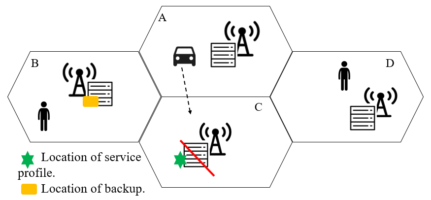
Figure 1: User mobility, and the placement of service profiles and backups in light of potential server failures in edge computing.

To take into account the potential failures and reduce the costs experienced by the user, a backup of the user’s service profile can be placed in the system. This way, if the server $l_{s}(t)$ at which the user’s service is placed at experiences a failure, the user will still be able to offload its job. As seen in Fig. 1, the vehicle moves from location A to C, and it’s service profile was pre-emptively placed at C. Although a server failure occured at C, the user is still able to offload its job computation, because a backup of the service profile was placed at B. We formulate a Markov Decision Process (MDP) in which the system state $s(t)\in S$ is $(l_{u}(t),l_{s}(t),f_{ind}(t),b_{ind}(t))$. $l_{u}$ is the user’s current location, $l_{s}$ is the location of the service, $f_{ind}$ is an indicator on whether the service is placed at a location with a server failure, and $b_{ind}$ indicates whether there currently is a backup in the system. At each timeslot $t$, the network operator takes action $a(t)=\{l_{s}(t+1),b_{u}(t+1)\}$ pre-emptively, before the user moves to the next location $l_{u}(t+1)$. This involves determining the placement location of the service $l_{s}(t+1)$, and the position of the backup in the system $b_{u}(t+1)\in\{0,1,...N,\text{no backup}\}$, where no backup refers to the choice of there not being a backup in the system. These decisions will directly impact the system state $s$ at the next timeslot.

Backup costs. There is a cost $B(t)$ incurred by storing the backup at a server. This cost is a sum of the backup migration cost and the backup storage cost, as it takes up space and prevents other content from being stored.

$${\color[rgb]{0.0,0.0,0.0}B}(t) =\sum_{j\in A}\rho_{j}\mathbbm{1}_{\{b_{u}(t)=j\}}$$ (3)

$$+\sum_{i\in A}\sum_{j\in A}m_{ij}\mathbbm{1}_{\{b_{u}(t-1)=i\}}\mathbbm{1}_{\{b_{u}(t)=j\}},$$

where $\rho_{j}$ is the storage cost at access point $j$. There is also a failure cost $F(t)$ incurred when there is a server failure at the location where the user’s service is placed at $(f_{ind}(t)=1)$, because the user’s task is not served within the task deadline.

$$F(t)=F\mathbbm{1}_{\{f_{ind}(t)=1\}}(\mathbbm{1}_{\{b_{u}(t)=\text{no backup}\}}\lor\mathbbm{1}_{\{b_{u}(t)=l_{s}(t)\}})$$ (4)

The failure cost is experienced at time $t$ when there is no backup in the system ($b_{u}(t)=\text{no backup}$), or when the placement of the backup $b_{u}(t)$ equals the location of the main service $l_{s}(t)$. Otherwise, if there is a backup placed, there will be no failure cost experience, and the cost will be much lower. Note, however, that the presence of failures themselves, i.e., $f_{ind}(t)$, is independent of the user actions.

Users move from one access point ($l_{u}(t)$) to another ($l_{t}(t+1)$) following their mobility distribution $m(l_{u}^{\prime}|l_{u})$, as mentioned in Subsection III-A. We let

$$h(\tilde{s}|s,a)=m(l_{u}^{\prime}|l_{u})Pr(a),$$ (5)

the product of the user’s mobility distribution and the probability that the network operator takes a particular action, where

$$\tilde{s}(t+1)=(l_{u}(t+1),l_{s}(t+1),b_{ind}(t+1))\in\tilde{S}$$ (6)

refers to the state record without the failure indicator $f_{ind}$. We let the set of this ”state records” be $\tilde{S}$. At each state $s$, there is a small probability of $\epsilon(s)$ (for example $\epsilon(s)=0.01$), that in the next timeslot, a server failure occurs, i.e. $f_{ind}=1$. We term states in which a server failure occurs as state set $T\subset S$, the “Rare event states”. With a larger probability of $1-\epsilon(s)$, no server failure occurs, i.e. $f_{ind}=0$. The non rare event states “Normal States” are defined as the set $S\backslash T$. Hence we have

$$s(t+1) =\tilde{s}(t+1)\cup f_{ind}(t+1)$$ (7)

$$=(l_{u}(t+1),l_{s}(t+1),b_{ind}(t+1),f_{ind}(t+1))\in S$$

Therefore, the overall state transition probability of the system can be expressed as

$$p(s^{\prime}|s,a)=\begin{cases}(1-\epsilon(s))h(\tilde{s}|s,a),&\text{if}\ s^{\prime}\notin T\\ \epsilon(s)h(\tilde{s}|s,a),&\text{if}\ s^{\prime}\in T,\end{cases}$$ (8)

In this study we focus on a single user, as the focus of our study is on rare events and rare events and failure aware resource allocation. We will consider optimizing service migration in a multi-user system in light of rare events in future work.

III-D Optimizing the Delay-Cost Trade-off in light of Anomalies

The network operator is interested in optimizing the placement and migration of the user’s service profile. In this study we have a specific focus on how long term service placements and backup storage decisions can be made, taking into account rare events such as server shutdowns which have an impact on the user experience and on the edge computing system resilience. We study the following problem:

$$\min_{\pi(s)} \mathbb{E}_{\pi}[\sum_{t}(w_{D}D(t)+w_{M}M(t)+w_{B}B(t)$$ (9)

$$+F(t))]$$

s.t. $$(l_{u}(t),l_{s}(t),f_{ind}(t),b_{ind}(t))\sim p(s^{\prime}|s,a).$$ (10)

$$\text{Eqs.}(\ref{eq:CommDelay1User}),(\ref{eq:switchingCost}),(\ref{eq:backupCost}),(\ref{eq:failureCost}).$$

In this problem we aim to minimize the expectation (over the policy $\pi$) of the sum of the delay, migration, storage and failure costs. The weights can be adjusted based on the priority given to the different costs. The decision variable $\pi(s,a)=\{P_{r}(a_{t}=a|s_{t}=s)\}$ is the network operator’s policy which indicates the probability it will take each action $a(t)=\{l_{s}(t+1),b_{u}(t+1)\}$ (service placement and backup storage decision) given the current state $s_{t}=(l_{u},l_{s},f_{ind},b_{ind})$. The first constraint indicates that the state dynamics follows the transition probability of the system in Eq. (8), incorporating rare event transitions, while the second and third constraints indicate the delay, migration, backup and failure costs respectively.

Proposition 1.

The number of migration path possibilities grows at least fast as $O(N^{T})$.

Proof.

For each timeslot $t$, there are $N$ possible locations to migrate a service profile. Since the service profile must be placed at a server each timeslot, the result follows. ∎

Deciding a migration path for the user across $T$ timeslots is similar to the shortest path problem, where the migration path possibilities grow at least as fast as $O(N^{T})$. At the same time, the network operator may not have information on the mobility distributions and the corresponding latency costs, making it difficult to solve the migration problem in a look-ahead manner. Thus, Markov Decision Processes and Reinforcement Learning have been used to derive service migration policies in the edge computing literature [11, 38, 18, 19]. Nevertheless, the difficulty in our problem further arises due to the fact we model occasional server failures, with a drastically distinct cost from normal events due to their impact on smooth and safe functioning of applications. As these failures occur at a low probability, and because reinforcement learning relies on past reward data, the learner may miss the importance of these rare events and be unable to learn an optimal policy adaptive to server failures. We introduce our solution in the next section.

IV Reinforcement learning in the presence of Server Failures

In this section, we present FIRE: Failure-adaptive Importance sampling for Rare Events, a reinforcement learning based framework to optimize service migration and the placement of backups in the edge computing system, in light of potential server failures. We define rare events formally in Subsection IV-A, introduce importance sampling in Subsection IV-B, present our importance sampling based algorithm (ImRE) and its proof in Subsections IV-C and IV-D respectively, and present an eligibility traces version of the algorithm (ETAA) for faster convergence in Subsection IV-E.

IV-A Rare Events And Their Impact On The Value Function

We are concerned with rare event states if they have a meaningful impact on the costs the user experiences. In other words, we are concerned if the rare event states collectively have a meaningful impact on the value function. The value function $V^{\pi}(s):S\rightarrow\mathbb{R}$ for the policy $\pi$ is the expected-return of state $s$, i.e. it indicates how “good” (cost wise) a state is (based on the discounted sum of future rewards), when policy $\pi$ is used. The discount factor $\gamma$ indicates how much the network operator cares about rewards in the distant future as opposed to rewards in the near future.

$$V^{\pi}(s)=\mathbb{E}_{a_{t},p(s^{\prime}|s,a)}\left[\sum_{t=1}^{\infty}\gamma^{k}r(s(t),a(t),a(t+1))|s_{0}=s\right],$$ (11)

where the reward (cost)

$$\begin{split}r(s(t),a(t),a(t+1))&=w_{D}D(t)+w_{M}M(t)\\ &+w_{B}B(t)+F(t)\end{split}$$ (12)

is the per-timeslot cost as defined in the objective function (9) of our optimization problem, under state transition probability $p(s^{\prime}|s,a)$. It is the solution to the recursive Bellman equation [35]:

$$V^{\pi}(s)=\sum_{a\in A}\pi(s,a)\sum_{s^{\prime}\in S}p(s^{\prime}|s,a)[r(s,a,s^{\prime})+\gamma V^{\pi}(s^{\prime})].$$ (13)

Defining $T^{\pi}(s)$ as the collective contribution of the rare states towards the value of state $s$ [20], given a fixed policy $\pi$, we have

$$T^{\pi}(s)=\epsilon(s)\sum_{a\in A}\sum_{\tilde{s}^{\prime}\in\tilde{S}}h(\tilde{s}^{\prime}|s,a)\pi(a|s)[r(s,a,s^{\prime})+\gamma V^{\pi}(s^{\prime})]$$ (14)

Likewise, defining $U^{\pi}(s)$ as the collective contribution of the non-rare states (states in $S\backslash T$) towards the value of state $s$, given a fixed policy $\pi$, we have :

$$U^{\pi}(s)=(1-\epsilon(s))\times$$ (15)

$$\sum_{a\in A}\sum_{\tilde{s}^{\prime}\in\tilde{S}}\pi(a|s)h(\tilde{s}^{\prime}|s,a)[r(s,a,s^{\prime})+\gamma V^{\pi}(s^{\prime})].$$

The Q-value (action-value) of a state action pair $(s,a)$ is the expected-return of taking action $a$ at state $s$, following policy $\pi$.

$$Q^{\pi}(s,a)=\mathbb{E}_{\pi}[\sum_{k=1}^{\infty}\gamma^{k}r(s(t),a(t),s(t+1))|s_{t}=s,a_{t}=a].$$ (16)

$$Q^{\pi}(s,a)=\sum_{s^{\prime}\in S}p(s^{\prime}|s,a)[r(s,a,s^{\prime})+\gamma\sum_{a^{\prime}\in A}\pi(a^{\prime}|s^{\prime})Q^{\pi}(s^{\prime},a^{\prime})]$$ (17)

The optimal policy will achieve the minimum cost and minimum value function:

$$Q^{*}(s,a)=\min_{\pi}Q^{\pi}(s,a).$$ (18)

We now give a formal definition of $T$, the set of rare states:

Definition 1.

A subset of states $T\subset S$ is called the Rare Event State Set if the following properties hold:

1. There exists $s\in S,s^{\prime}\in T$ for which $p(s^{\prime}|s,a)>0$.

2. Let $T^{\pi}(s)$ denote the contribution of the rare states towards the value of state $s$, according to Eq. (14). For a given policy $\pi$, there exists $s\in S$ for which

$$|T^{\pi}(s)|\gg 0$$ (19)

The first property means that transition to the rare event state set $T$ is possible. The second property means that the rare event states in $T$ collectively have a meaningful (sizeable) impact on the value function. Intuitively, what this property means is that the rare event states collectively have a sizeable impact on the reward (cost) experienced by the user.

IV-B Importance Sampling

In this subsection we introduce the concept of importance sampling, an important component of our framework FIRE, which helps the network operator derive an optimal service migration and backup policy in light of potential rare events.

When we are trying to calculate the expectation of a function $f(x)$, and the true distribution $p$ is difficult to sample from, importance sampling is the process of sampling from another distribution $q$, instead of the true distribution $p$ [39]. In this scenario, the expectation of $f(x)$ can be estimated as

$$E[f(x)] =\int f(x)p(x)dx$$ (20)

$$=\int f(x)\frac{p(x)}{q(x)}q(x)dx$$ (21)

$$\approx\frac{1}{n}\sum_{i}f\left(x_{i}\right)\frac{p\left(x_{i}\right)}{q\left(x_{i}\right)}.$$ (22)

When $q$ is well crafted, variance in the value estimates will be reduced. The use of importance sampling in temporal difference (TD) based reinforcement learning was proposed in [34], in which the state transition probabilities followed another distribution $q(s^{\prime}|s,a)$ rather than the true $p(s^{\prime}|s,a)$. Unlike their work which estimates the value function given a fixed policy, in our work we propose an importance sampling based q-learning algorithm in which the policy is constantly changing until the optimal policy is reached.

For our service migration and backup placement problem, we will sample the rare events at a higher rate than they are expected to occur, to help the model learn an optimal policy in light of these server failures. The importance sampling correction weight $w(s,a,s^{\prime})$ will be defined by

$$w(s,a,s^{\prime})\leftarrow\begin{cases}\epsilon(s)/\hat{\epsilon}(s),&\text{if}\ s^{\prime}\in T,\\ (1-\epsilon(s))/(1-\hat{\epsilon}(s)),&\text{if}\ s^{\prime}\notin T,\end{cases}$$ (23)

where $\epsilon(s)$ is the actual rare event probability distribution at state $s$ (the probability that we next visit a rare event state after state $s$), and $\hat{\epsilon}(s)$ is the “proposal probability distribution” the rare events are sampled at, from state $s$. $1-\epsilon(s)$ is the probability that $s^{\prime}$ is a non-rare event state, and the importance sampling correction weight will be $(1-\epsilon(s))/(1-\hat{\epsilon}(s))$. The importance sampling correction weights $w(s,a,s^{\prime})$ will be used in our algorithm in Subsection IV-C.

IV-C ImRE: Q-Learning in Light of Rare Events

In this subsection, we present our importance sampling based failure-adaptive algorithm. Our algorithm is a simulator which trains an optimal service migration and backup placement policy in light of rare events. We use a simulator in order to avoid the large failure costs experienced during server failures in online scenarios. Our simulator performs importance sampling and increases the rare event probabilities from $\epsilon(s)$ to $\hat{\epsilon}(s)$. The transition probabilities $h(\tilde{s}|s,a)$, which is mostly dependent on the user mobility probabilities (Eq. (5)), can be obtained from historical data. The converged policy trained by the simulator is then applied to online scenarios, in which rare events happen at their natural probabilities. We use importance sampling because if rare events such as server failures are sampled at their natural probabilities, the reinforcement learning algorithm is not able to converge to the optimal policy as it may decide that the storage cost isn’t worth having backups. This can be catastrophic in the event of failures. In our numerical simulations in Section VII, we show that unlike our algorithm, a traditional reinforcement learning algorithm is unable to train an optimal policy which avoids experiencing high cost in the event of failures (Figs. 3 and 4).

Idea behind algorithm: Firstly, we discuss how we obtain the proposed probability distribution $\hat{\epsilon}(s)$ at which rare events are sampled at, given that the actual rare event probability distribution is $\epsilon(s)$. We want to sample rare events at a rate proportional to the contribution they have to the value of state $s$. For example, using something like $\hat{\epsilon}(s)=\frac{T^{\pi}(s)}{T^{\pi}(s)+U^{\pi}(s)}$. $T^{\pi}(s)$ and $U^{\pi}(s)$ (Eqs. (14) and (15)) were introduced in [20], and defined with respect to fixed policies $\pi$. Recall that $T^{\pi}(s)$ is the collective contribution of the rare states towards the value of state $s$, given a fixed policy $\pi$, and $U^{\pi}(s)$ is the collective contribution of the non-rare states (states in $S\backslash T$) towards the value of state $s$, given a fixed policy $\pi$. Unlike the algorithm in [20] whose aim was policy evaluation in light of importance sampling and involved a fixed policy, here we are learning an optimal policy $\pi^{*}$ through Q-learning. Therefore, to obtain $\hat{\epsilon}(s)$, we define $T(s,a)$ as the contribution of the rare states $s^{\prime}\in T$ towards the Q-value of the state action pair $(s,a)$, and $U(s,a)$ as the contribution of the normal states $s^{\prime}\in S\backslash T$ towards the Q-value of the state action pair $(s,a)$:

$$T(s,a)=\epsilon(s)\sum_{\tilde{s}^{\prime}\in\tilde{S}}h(\tilde{s}^{\prime}|s,a)[r(s,a,s^{\prime})+\gamma\max_{b}Q(s^{\prime},b)]$$ (24)

$$U(s,a)=(1-\epsilon(s))\sum_{\tilde{s}^{\prime}\in\tilde{S}}h(\tilde{s}^{\prime}|s,a)[r(s,a,s^{\prime})+\gamma\max_{b}Q(s^{\prime},b)]$$ (25)

where $s^{\prime}=\tilde{s}^{\prime}\cup f_{ind}$, and obtaining $\max_{b}Q(s^{\prime},b)$ follows the policy $\pi$. With this, we have the relationship $T(s,a)+U(s,a)=Q(s,a).$ A potential update equation for $T(s,a)$ would be $T(s,a)\leftarrow(1-\alpha_{T})T(s,a)+\alpha_{T}\epsilon(s)(r(s,a,s^{\prime})+\gamma\max_{b}Q(s^{\prime},b))$, where $\alpha_{T}$ is the learning rate.

Nevertheless, updating at the state action $(s,a)$ level may lead to slower convergence, especially when the number of access points increase leading to an exponential increase in the number of state and action combinations. For example, when there are 9 access points, there will be 360 states and 90 actions, leading to 32400 state action combinations. We can reduce this complexity by exploiting our earlier observation that the probability of rare events (i.e., server failures) happening is independent of the actions chosen. Therefore, we propose updating $T$ (the contributions of the rare events towards the Q-value) and $U$ (the contribution of the non-rare events towards the Q-value) at the state level:

$$\begin{split}&T(s)=\\ &\epsilon(s)\sum_{a\in A}\sum_{\tilde{s}^{\prime}\in S}\pi(a|s)h(\tilde{s}^{\prime}|s,a)[r(s,a,s^{\prime})+\gamma\max_{b}Q(s^{\prime},b)]\end{split}$$ (26)

$$\begin{split}&U(s)=(1-\epsilon(s))\times\\ &\sum_{a\in A}\sum_{\tilde{s}^{\prime}\in S}\pi(a|s)h(\tilde{s}^{\prime}|s,a)[r(s,a,s^{\prime})+\gamma\max_{b}Q(s^{\prime},b)]\end{split}$$ (27)

The relationship $U(s)+T(s)=\sum_{a}Q(s,a)\pi(a|s)$ holds.

To help us obtain the importance sampling rare event rate $\hat{\epsilon}(s)$, We will use the following update equations for $T(s)$ and $U(s)$ in our algorithm:

$$T(s)\leftarrow(1-\alpha_{T})T(s)+\alpha_{T}\epsilon(s)(r(s,a,s^{\prime})+\gamma\max_{b}\hat{Q}(s^{\prime},b))$$ (28)

$$U(s) \leftarrow(1-\alpha_{U})U(s)$$ (29)

$$+\alpha_{U}(1-\epsilon(s))(r(s,a,s^{\prime})+\gamma\max_{b}\hat{Q}(s^{\prime},b))$$

respectively. Based on these, we will calculate the rare event importance sampling rate $\hat{\epsilon}(s)$ as follows:

$$\hat{\epsilon}(s)\leftarrow min(max(\delta,\frac{|T(s)|}{|T(s)|+|U(s)|}),1-\delta).$$ (30)

The bounds $(\delta,1-\delta)$ help to ensure sufficient rare event sampling.

Importance sampling and correction: As importance sampling of rare events takes place according to $\hat{\epsilon}(s)$, $\hat{p}(s^{\prime}|s,a)$ is the transition probability in our algorithm which incorporates importance sampling. $\hat{p}(s^{\prime}|s,a)=\begin{cases}(1-\hat{\epsilon}(s))h(\tilde{s}|s,a),&\text{if}\ s^{\prime}\notin T\\ \hat{\epsilon}(s)h(\tilde{s}|s,a),&\text{if}\ s^{\prime}\in T,\end{cases}$ where $\tilde{s}$ is the intermediate state, as mentioned in Eq. (6).

Because the rare events are sampled at the probability $\hat{\epsilon}$ instead of their actual probability $\epsilon$. Therefore, we need a method of correction, in order to learn the optimal policy for the original system with transition probability $p(s^{\prime}|s,a)$ (Eq. (8)). Importance sampling correction weights will be used, when obtaining the temporal-difference (TD) error in Q-learning. The importance sampling correction weights will be $\epsilon(s)/\hat{\epsilon}(s)$ when the next state after $s$ is a rare event, and $(1-\epsilon(s))/(1-\hat{\epsilon}(s))$ when the next state after $s$ is not a rare event, as seen in Eq. (23). The TD error will be

$$w_{t}(r(s,a,s^{\prime})+\gamma\max_{b}\hat{Q}(s^{\prime},b))-\hat{Q}(s,a),$$ (31)

instead of the traditional Q-learning TD error $r(s,a,s^{\prime})+\gamma\max_{b}\hat{Q}(s^{\prime},b)-\hat{Q}(s,a)$.

Algorithm description: The algorithm is presented in Algorithm 1 (ImRE). Firstly, we initialise the Q-values $\hat{Q}(s,a)$ to be $0$ (for all state action pairs), $\hat{T}(s)$ and $\hat{U}(s)$ to be $0$ (for all states), and $\hat{\epsilon}(s)$ to be $\frac{1}{2}$ for all states. We also initialise the learning rates $\alpha^{t},\alpha^{t}_{T},\alpha^{t}_{U}$. For every timeslot, the importance sampling rare event probability $\hat{\epsilon}(s)$ will determine whether or not a rare-event (failure) occurs. Thereafter, the rest of the state transition will occur according to the probability distribution $h(\tilde{s}|s,a)$, where $\tilde{s}(t)=(l_{u}(t),l_{s}(t),b_{ind}(t))$. This would result in a new state $s^{t+1}$, and a reward value $r^{t+1}=r(s^{t},a^{t},s^{t+1})$ (line 4). Based on the next state $s^{t+1}$, a new action is selected according to the $\beta$-greedy policy (lines 5-6), which is the same as the traditional $\epsilon$-greedy policy in Q-learning, where with probability $\beta$ the greedy action is selected and with probability $1-\beta$ a random action is selected, for exploration. We call it $\beta$-greedy to avoid confusion with our rare event probability $\epsilon$.

Next, we obtain the importance weight $w_{t}$ for this timeslot. The importance weight is the actual probability divided by the importance sampling - edited probability (line 7). The temporal-difference (TD) error $\triangle_{t}$ will be updated (line 8), while error corrected by the importance sampling weight $w_{t}$. With the TD-error, we update $\hat{Q}(s^{t},a^{t})$, the Q-value for state $s^{t}$ and action $a^{t}$ (line 9). The size of update is determined by the learning rate $\alpha^{t}$. We then update either $T(s^{t})$ or $U(s^{t})$, depending on whether the next state $s^{t+1}$ is a rare event state or not (lines 10-14). Finally, the importance sampling rare events probability $\hat{\epsilon}(s^{t})$ is updated in line 15, according to $\frac{|T(s^{t})|}{|T(s^{t})|+|U(s^{t})|}$, and bounded by $\delta$ and $1-\delta$. The process iterates for every timeslot, until we have achieved convergence.

Algorithm 1 ImRE: Importance Sampling Q-Learning for Rare Events

1:Initialise: $\hat{Q}(s,a)$ randomly, $\hat{T}(s),\hat{U}(s)\leftarrow 0$, $\hat{\epsilon}(s)\leftarrow\frac{1}{2},\alpha^{t},\alpha^{t}_{T},\alpha^{t}_{U}.$

2:Select the initial state $s^{0}$ and action $a^{0}$.

3:for all timeslots $t$ do

4:     $\hat{\epsilon}(s^{t})$ determines if an rare event happens. Thereafter, sample according to $h(\tilde{s}|s,a)$. The new state $s^{t+1}$ and a reward value $r^{t+1}=r(s^{t},a^{t},s^{t+1})$ is observed.

5:     $a^{t+1}\leftarrow\beta-\text{greedy}(s^{t+1}).$

6:     $a^{*}\leftarrow\text{argmax}_{b}\hat{Q}(s^{t+1},b).$

7:     $w_{t}\leftarrow\begin{cases}\epsilon(s^{t})/\hat{\epsilon}(s^{t}),&\text{if}\ s^{t+1}\in T.\\ (1-\epsilon(s^{t}))/(1-\hat{\epsilon}(s^{t})),&\text{if}\ s^{t+1}\notin T.\end{cases}$

8:     $\triangle_{t}\leftarrow w_{t}(r^{t+1}+\gamma\hat{Q}(s^{t+1},a^{*}))-\hat{Q}(s^{t},a^{t})$

9:     $\hat{Q}(s^{t},a^{t})\leftarrow\hat{Q}(s,a)+\alpha^{t}\triangle_{t}$.

10:     if $s^{t+1}\in T$ then

11:         $T(s^{t})\leftarrow(1-\alpha^{t}_{T})T(s^{t})+\alpha^{t}_{T}\epsilon(s^{t})(r^{t+1}+\gamma\hat{Q}(s^{t+1},a^{*}))$

12:     else

13:         $U(s^{t})\leftarrow(1-\alpha^{t}_{U})U(s^{t})+\alpha^{t}_{U}(1-\epsilon(s^{t}))(r^{t+1}+\gamma\hat{Q}(s^{t+1},a^{*}))$

14:     end if

15:     $\hat{\epsilon}(s^{t})\leftarrow min(max(\delta,\frac{|T(s^{t})|}{|T(s^{t})|+|U(s^{t})|}),1-\delta)$

16:end for

Our algorithm works for the scenario where $\exists s,\text{s.t.}|T(s)|\gg 0$. See Statement 2 in the definition of rare events in Definition 1. In this scenario, the rare events have a sizeable contribution to the Q-value of at least one other state action pair $(s,a)$. When this condition is met, the rare events collectively have a sufficient impact on the reward/cost of the system, meaning that the cost of rare events to the users and network operator is sufficiently high. On the other hand, when the condition is not met, the cost of rare events to the users and network operator is not sufficiently high enough, resulting in less of a need to optimize resource allocation in light of rare events.

IV-D Proofs of Boundedness and Convergence to Optimality

In this subsection, we prove the convergence of ImRE, our importance sampling based Q-learning algorithm (Algorithm 1). Firstly, we show that the sequence of updates in Algorithm 1 are bounded, in the following theorem.

Theorem 2.

For stepsizes following the conditions $\sum_{t}\alpha(t)=\infty$ and $\sum_{t}\alpha^{2}(t)\leq\infty$, and discount factor $\gamma\in(0,1)$, the sequence of the $\hat{Q}$ updates in Algorithm 1 is bounded, with probability 1.

Proof.

Algorithm 1’s update equation is

$$\hat{Q}(s^{t},a^{t})\leftarrow\hat{Q}(s^{t},a^{t})+\alpha[w_{t}(r^{t+1}+\gamma\hat{Q}(s^{t+1},a^{*}))-\hat{Q}(s^{t},a^{t})],$$ (32)

where $a^{*}=\text{argmax}_{b}\hat{Q}(s^{t+1},b)$.

We rewrite Algorithm 1’s update equation through adding and subtracting the term $\sum_{s^{\prime}\in S}\hat{p}(s^{\prime}|s^{t},a^{t})(r^{t}(s^{t},a^{t},s^{\prime})+\gamma\max_{y}\hat{Q}^{t}(s^{\prime},y))$, as follows:

$$\begin{split}&\hat{Q}^{t+1}(s^{t},a^{t})=\hat{Q}^{t}(s^{t},a^{t})+\alpha^{t}[\sum_{s^{\prime}\in S}\hat{p}(s^{\prime}|s^{t},a^{t})(r^{t}(s^{t},a^{t},s^{\prime})\\ &+\gamma\max_{y}\hat{Q}^{t}(s^{\prime},y))-\hat{Q}^{t}(s^{t},a^{t})]+\alpha^{t}[\frac{\epsilon(s^{t})}{\hat{\epsilon}(s^{t})}(r^{t}(s^{t},a^{t},s^{t+1})\\ &+\gamma\hat{Q}^{t}(s^{t+1},a^{*}))-\sum_{s^{\prime}\in S}\hat{p}(s^{\prime}|s^{t},a^{t})(r^{t}(s^{t},a^{t},s^{\prime})\\ &+\gamma\max_{y}\hat{Q}^{t}(s^{\prime},y))].\end{split}$$ (33)

This can be rewritten as

$$\begin{split}&\hat{Q}^{t+1}(s,a)=\hat{Q}^{t}(s,a)+\alpha^{t}[F_{s,a}(\hat{Q}^{t})\\ &-\hat{Q}^{t}(s^{t},a^{t})+M_{s}(t)],\end{split}$$ (34)

for all $(s,a)$, where $F_{s,a}=[F_{s1,a1},...,F_{|S\times A|}]^{T}$ is defined by

$$\begin{split}&F_{s,a}(\hat{Q}^{t}(s,a))\\ &=\sum_{s^{\prime}\in S}\hat{p}(s^{\prime}|s,a)(r^{t}(s,a,s^{\prime})+\gamma\max_{y}\hat{Q}^{t}(s^{\prime},y)),\end{split}$$ (35)

and $\{M(t)\},M(t)=[M_{1,1}(t),M_{1,2}(t),...,M_{|S\times A|}(t)]$ is a sequence of random vectors in $\mathbb{R}^{|S\times A|}$ satisfying

$$\mathbb{E}[M_{m}(t)|m<t]=0$$ (36)

$$||M(t)||\leq K(1+||\hat{Q}^{t}||)$$ (37)

for some constant $K>0$. Specifically, $M(t)$ will be the vector with all zeros except for the $t$-th element, which is given by the term in the second square bracket in Eq. (33). $||M(t)||$ is bounded because the probabilities $\epsilon(s^{t})$ and $1-\epsilon(s^{t})$ are fixed, while $\hat{\epsilon}(s^{t})$ and hence $1-\hat{\epsilon}(s^{t})$ are bounded in our algorithm (line 15). This results in the importance weight $w^{t}$ (Eq. (23)) being bounded.

We show that the property $||F(\hat{Q})||_{\infty}\leq b||\hat{Q}||_{\infty}+d$ holds, where $||\quad||_{\infty}$ is the supremum norm.

$$||F(\hat{Q})||_{\infty}$$ (38)

$$=\max_{i,a}|\sum_{s^{\prime}\in S}\hat{p}(s^{\prime}|i,a)(r(i,a,s^{\prime})+\gamma\max_{y}\hat{Q}(s^{\prime},y))|$$ (39)

$$\begin{split}&\leq\max_{i,a}[|\sum_{s^{\prime}\in S}\hat{p}(s^{\prime}|i,a)r(i,a,s^{\prime})|\\ &+|\sum_{s^{\prime}\in S}\hat{p}(s^{\prime}|i,a)\gamma\max_{y}\hat{Q}(s^{\prime},y)|]\end{split}$$ (40)

$$\begin{split}&\leq\max_{i,a}|\sum_{s^{\prime}\in S}\hat{p}(s^{\prime}|i,a)r(i,a,s^{\prime})|\\ &+\gamma\max_{i,a}|\sum_{s^{\prime}\in S}\hat{p}(s^{\prime}|i,a)\max_{z,y}\hat{Q}(z,y)|\end{split}$$ (41)

$$\begin{split}&=\max_{i,a}|\sum_{s^{\prime}\in S}\hat{p}(s^{\prime}|i,a)r(i,a,s^{\prime})|\\ &+\gamma\max_{i,a}\sum_{s^{\prime}\in S}\hat{p}(s^{\prime}|i,a)||\hat{Q}||_{\infty}\end{split}$$ (42)

$$=b||\hat{Q}||_{\infty}+d$$ (43)

where $b=\gamma\max_{i,a}\sum_{s^{\prime}\in S}\hat{p}(s^{\prime}|i,a)=\gamma<1$ and $d=\max_{i,a}|\sum_{s^{\prime}\in S}\hat{p}(s^{\prime}|i,a)r(i,a,s^{\prime})|=\max_{i,a}|r(i,a,s^{\prime})|$. The first inequality (from Eq. (39) to (40)) is true by the triangle inequality.

Therefore, by Theorem 1 of [40] on stochastic approximation algorithms, the sequence of $\hat{Q}$ updates in Algorithm 1 is bounded, with probability 1. ∎

The main idea of the above proof is as follows. Firstly, we add and subtract the term $\sum_{s^{\prime}\in S}\hat{p}(s^{\prime}|s^{t},a^{t})(r^{t}(s^{t},a^{t},s^{\prime})+\gamma\max_{y}\hat{Q}^{t}(s^{\prime},y))$ in Algorithm 1’s update equation. Next, we rewrite the equation in the form of $\hat{Q}^{t+1}(s,a)=\hat{Q}^{t}(s,a)+\alpha^{t}[F_{s,a}(\hat{Q}^{t})-\hat{Q}^{t}(s^{t},a^{t})+M_{s}(t)]$. We describe why $M_{s}(t)$ is bounded. Finally, to show that the conditions for the sequence to be bounded are met (Theorem 1 of [40] on stochastic approximation algorithms), we show that $||F(\hat{Q})||_{\infty}\leq b||\hat{Q}||_{\infty}+d$, where $b<1$.

Next, to help us prove that our algorithm ImRE converges to optimality, we invoke the following theorem from [41]:

Corollary 3.

The random process $\{\triangle_{t}\}$ taking values in $\mathbb{R}^{n}$ and defined as

$$\triangle_{t+1}(x)=(1-\alpha_{t}(x))\triangle_{t}(x)+\alpha_{t}F_{t}(x)$$ (44)

converges to zero with probability 1 when the following assumptions hold:

$$0\leq\alpha_{t}\leq 1,\sum_{t}\alpha_{t}(x)=\infty\ \text{and}\sum_{t}\alpha^{2}_{t}(x)<\infty.$$

$$||\mathbb{E}[F_{t}(x)]||\leq\gamma||\triangle_{t}||,\text{where}\ \gamma<1.$$

$$var[F_{t}(x)]\leq C(1+||\triangle_{t}||^{2}),\ \text{for}\ C>0.$$

Proof.

See [41]. ∎

In the following theorem, we show that our algorithm converges, and that it converges to the optimal policy.

Theorem 4.

If the MDP is unichain for $\epsilon\in(\delta,1-\delta)$, for stepsizes following the conditions $0\leq\alpha_{t}\leq 1$, $\sum_{t}\alpha_{i}(t)=\infty$ and $\sum_{t}\alpha_{i}^{2}(t)\leq\infty$, and discount factor $\gamma\in(0,1)$, Algorithm 1 converges to the optimal policy $Q^{*}$.

Proof.

Algorithm 1’s update equation is

$$\begin{split}&\hat{Q}^{t+1}(s^{t},a^{t})\leftarrow\hat{Q}^{t}(s^{t},a^{t})+\alpha[w_{t}(r^{t+1}+\gamma\hat{Q}^{t}(s^{t+1},a^{*}))\\ &-\hat{Q}^{t}(s^{t},a^{t})],\end{split}$$ (45)

where $a^{*}=\text{argmax}_{b}\hat{Q}(s^{t+1},b)$.

By definition, the optimal policy $Q^{*}$ of the true system with transition probability $p(s^{\prime}|s,a)$ is a fixed point of the Bellman optimality equation:

$$Q^{*}(s,a)=\sum_{s^{\prime}\in S}p(s^{\prime}|s,a)[r(s,a,s^{\prime})+\gamma\max_{b}Q^{*}(s^{\prime},b)].$$ (46)

$\hat{p}(s^{\prime}|s,a)$ is the transition probability in our simulator which incorporates importance sampling. $\hat{p}(s^{\prime}|s,a)=\begin{cases}(1-\hat{\epsilon}(s))h(\tilde{s}|s,a),&\text{if}\ s^{\prime}\notin T\\ \hat{\epsilon}(s)h(\tilde{s}|s,a),&\text{if}\ s^{\prime}\in T,\end{cases}$ as importance sampling of rare events takes place according to $\hat{\epsilon}(s)$. Without loss of generality, when we look at the case where $s^{\prime}$ is a rare state ($s^{\prime}\in T$), we have

$$\begin{split}\hat{p}(s^{\prime}|s,a)w_{t}(s)&=\hat{\epsilon}(s)h(\tilde{s}|s,a)\frac{\epsilon(s)}{\hat{\epsilon}(s)}\\ &=p(s^{\prime}|s,a),\end{split}$$ (47)

the actual transition probability of the system. Therefore, since $p(s^{\prime}|s,a)=\hat{p}(s^{\prime}|s,a)w_{t}(s)$, the optimal policy $Q^{*}$ is a fixed point of the following equation with our simulator’s transition probability $\hat{p}(s^{\prime}|s,a)$ and the importance sampling correction weight $w_{t}(s)$:

$$Q^{*}(s,a)=\sum_{s^{\prime}\in S}\hat{p}(s^{\prime}|s,a)w_{t}(s)[r(s,a,s^{\prime})+\gamma\max_{b}Q^{*}(s^{\prime},b)].$$ (48)

We let the operator $\mathbf{H}$ for a generic function $\hat{Q}_{i}$ be defined as

$$(\mathbf{H}\hat{Q})(s,a)=\sum_{s^{\prime}\in S}\hat{p}(s^{\prime}|s,a)w_{t}(s)[r(s,a,s^{\prime})+\gamma\max_{b}\hat{Q}(s^{\prime},b)].$$ (49)

We have shown above that $\mathbf{H}Q^{*}=Q^{*}$. Now we show that $\mathbf{H}$ is a contraction mapping. Note that both $\hat{p}(s^{\prime}|s,a)$ and $w_{t}(s)$ are functions of $\hat{Q}$, because they are functions of $\hat{\epsilon}$, which is obtained as a function of $\hat{Q}$ (lines 10-15). Nevertheless, we are able to prove contraction mapping because the product $\hat{p}(s^{\prime}|s,a)(\hat{Q})\times w_{t}(s(\hat{Q}))$ is the true transition probability $p(s^{\prime}|s,a)$.

$$||\mathbf{H}\hat{Q}_{1}-\mathbf{H}\hat{Q}_{2}||_{\infty}$$ (50)

$$=\max_{s,a}|\sum_{s^{\prime}}\hat{p}(\hat{Q}_{1})(s^{\prime}|s,a)w_{t}(s(\hat{Q}_{1}))[r(s,a,s^{\prime})$$ (51)

$$+\gamma\max_{b}\hat{Q}_{1}(s^{\prime},b)]-\sum_{s^{\prime}}\hat{p}(\hat{Q}_{2})(s^{\prime}|s,a)w_{t}(s(\hat{Q}_{2}))[r(s,a,s^{\prime})$$ (52)

$$+\gamma\max_{b}\hat{Q}_{2}(s^{\prime},b)]|$$ (53)

$$=\max_{s,a}|\sum_{s^{\prime}}p(s^{\prime}|s,a)[r(s,a,s^{\prime})+\gamma\max_{b}\hat{Q}_{1}(s^{\prime},b)]$$ (54)

$$-\sum_{s^{\prime}}p(s^{\prime}|s,a)[r(s,a,s^{\prime})+\gamma\max_{b}\hat{Q}_{2}(s^{\prime},b)]|$$ (55)

$$\begin{split}&=\max_{i,a}|\sum_{s^{\prime}\in S}p(s^{\prime}|i,a)\gamma[\max_{y}\hat{Q}_{1}(s^{\prime},y)-\max_{y}\hat{Q}_{2}(s^{\prime},y)]|\end{split}$$ (56)

$$\leq\max_{i,a}\gamma\sum_{s^{\prime}\in S}p(s^{\prime}|i,a)|\max_{y}\hat{Q}_{1}(s^{\prime},y)-\max_{y}\hat{Q}_{2}(s^{\prime},y)|$$ (57)

$$\leq\max_{i,a}\gamma\sum_{s^{\prime}\in S}p(s^{\prime}|i,a)|\max_{y}|\hat{Q}_{1}(s^{\prime},y)-\hat{Q}_{2}(s^{\prime},y)||$$ (58)

$$\leq\max_{i,a}\sum_{s^{\prime}\in S}p(s^{\prime}|i,a)\max_{z,y}|\hat{Q}_{1}(z,y)-\hat{Q}_{2}(z,y)|$$ (59)

$$=\max_{i,a}\gamma\sum_{s^{\prime}\in S}p(s^{\prime}|i,a)||\hat{Q}_{1}-\hat{Q}_{2}||_{\infty}$$ (60)

$$=\gamma||\hat{Q}_{1}-\hat{Q}_{2}||_{\infty},$$ (61)

where $\gamma\in[0,1)$ according to the theorem conditions. The first inequality is true by the triangle inequality. The second inequality holds because $\max_{x}f(x)-\max_{x}g(x)\leq\max_{x}|f(x)-g(x)|$. Hence, we have shown that operator $H$ is a contraction mapping.

To prove convergence of our algorithm, we use the result from Corollary 3. Firstly, we subtract $Q^{*}(s^{t},a^{t})$ from both sides of Eq. (45), and letting $\triangle_{t}(s,a)=\hat{Q}^{t}(s,a)-Q^{*}(s,a)$, we have:

$$\triangle_{t+1}(s^{t},a^{t})=(1-\alpha^{t})\triangle_{t}(s^{t},a^{t})$$ (62)

$$+\alpha^{t}[w^{t}(r^{t+1}+\gamma\max_{b}\hat{Q}^{t}(s^{t+1},b))-Q^{*}(s^{t},a^{t})].$$ (63)

where $r^{t+1}=r(s^{t},a^{t},s^{t+1})$.

Let

$$G_{t}(s,a)=w^{t}[r(s,a,X(s,a))+\gamma\max_{b}\hat{Q}^{t}(X(s,a),b)]$$

$$-Q^{*}(s,a),$$

where $X(s,a)$ is a random sample obtained from the markov chain with state space $S$ and transition probability $\hat{p}(s^{\prime}|s,a)$ (the importance sampling modified transition probability). Taking the expectation, we have

$$\mathbb{E}[G_{t}(s,a)]=\sum_{s^{\prime}\in S}\hat{p}(s^{\prime}|s,a)w^{t}(s)[r(s,a,s^{\prime})$$

$$+\gamma\max_{b}\hat{Q}^{t}(s,b)]-Q^{*}(s,a)$$

$$=\mathbf{H}\hat{Q}^{t}(s,a)-Q^{*}(s,a)$$

$$=\mathbf{H}\hat{Q}^{t}(s,a)-\mathbf{H}Q^{*}(s,a).$$

The last equality holds because $Q^{*}$ is a fixed point of operator $\mathbf{H}$, as we have shown in Eqs. (48) and (49). Since we have shown that $\mathbf{H}$ is a contraction mapping above, we have

$$||\mathbb{E}[G_{t}(s,a)]||_{\infty}\leq\gamma||\hat{Q}^{t}(s,a)-Q^{*}||_{\infty}=\gamma||\triangle_{t}||_{\infty}.$$ (64)

It remains to show that $\textbf{var}[F_{t}(x)]\leq C(1+||\triangle_{t}||^{2}),\text{for}\ C>0$, where var refers to the variance.

$$\textbf{var}[G_{t}(s,a)]$$

$$=\mathbb{E}[\Bigl{(}w^{t}[r(s,a,X(s,a))+\gamma\max_{b}\hat{Q}^{t}(X(s,a),b)]-Q^{*}(s,a)$$

$$-\mathbf{H}\hat{Q}^{t}(s,a)+Q^{*}(s,a)\Bigr{)}^{2}]$$

$$=\mathbb{E}[\Bigl{(}w^{t}[r(s,a,X(s,a))+\gamma\max_{b}\hat{Q}^{t}(X(s,a),b)]$$

$$-\mathbf{H}\hat{Q}^{t}(s,a)\Bigr{)}^{2}]$$

$$=\textbf{var}\Bigl{(}w^{t}[r(s,a,X(s,a))+\gamma\max_{b}\hat{Q}^{t}(X(s,a),b)]\Bigr{)}$$

Since $w^{t}$ and $r$ are bounded, we have

$$\mathbf{var}[G_{t}(s,a)]\leq C(1+||\triangle_{t}||^{2}_{\infty})$$ (65)

for some constant $C>0$. With this, we have shown the convergence of Algorithm ImRE. ∎

The main idea of the above proof is as follows. Firstly, we show that the optimal policy of the true system is not only a fixed point of the Bellman optimality equation with the system’s true transition probability $p(s^{\prime}|s,a)$, but also a fixed point of the following equation with our simulator’s transition probability $\hat{p}(s^{\prime}|s,a)$ and the importance sampling correction weight $w_{t}(s)$: $Q^{*}(s,a)=\sum_{s^{\prime}\in S}\hat{p}(s^{\prime}|s,a)w_{t}(s)[r(s,a,s^{\prime})+\gamma\max_{b}Q^{*}(s^{\prime},b)].$ We define the operator $\mathbf{H}\hat{Q}=\sum_{s^{\prime}\in S}\hat{p}(s^{\prime}|s,a)w_{t}(s)[r(s,a,s^{\prime})+\gamma\max_{b}\hat{Q}(s^{\prime},b)]$, and show that $\textbf{H}\hat{Q}$ is a contraction mapping, using the fact that $\hat{p}(s^{\prime}|s,a)w_{t}(s)=p(s^{\prime}|s,a)$. Next, we rewrite the update equation of Algorithm 1, such that it fits the form of Eq. (44) in Corollary 3, on the convergence of random processes. We then prove that the following conditions of Corollary 3 hold: $||\mathbb{E}[F_{t}(x)]||\leq\gamma||\triangle_{t}||,\text{where}\ \gamma<1,$ and $var[F_{t}(x)]\leq C(1+||\triangle_{t}||^{2}),\ \text{for}\ C>0.$

IV-E Eligibility Traces

To speed up convergence for the tabular Q learning algorithm, we propose another variant of Algorithm 1 using eligibility traces. This algorithm is a combination of our proposed importance sampling based Q-learning Algorithm 1 and Watkin’s $Q(\lambda)$ [42], which is an algorithm which combines Q-learning with eligibility traces.

Algorithm 2 ETAA: Eligibility Traces Rare Events-Adaptive Algorithm

1:Initialise: Same variables as Algorithm 1, along with eligibility traces $e(s,a)$.

2:Select the initial state $s^{0}$ and action $a^{0}$.

3:for all timeslots $t$ do

4:     The procedure follows that of Algorithm 1.

5:     When we visit $s^{t}$ and take action $a^{t}$, $e(s^{t},a^{t})\leftarrow e(s^{t},a^{t})+1.$

6:     $a^{t+1}\leftarrow\beta-\text{greedy}(s^{t+1}).$

7:     $a^{*}\leftarrow\text{argmax}_{b}\hat{Q}(s^{t+1},b).$

8:     if  $\hat{Q}(s^{t+1},a^{*})=\hat{Q}(s^{t+1},a^{t+1})$ then

9:         $a^{*}\leftarrow a^{t+1}$

10:     end if

11:     for all $(s,a)$ do

12:         $\hat{Q}(s,a)\leftarrow\hat{Q}(s,a)+\alpha e(s,t)\triangle_{t}$.

13:         if $a^{t+1}=a^{*}$ then

14:              $e(s,a)\leftarrow\gamma\lambda e(s,a)w_{t}$

15:         else

16:              $e(s,a)\leftarrow 0.$

17:         end if

18:     end for

19:end for

The details are in Algorithm 2. In this algorithm, $\hat{Q}(s,a)$ is updated for many combinations of $(s,a)$, at every time-slot, which helps to speed up convergence. Firstly, when we visit state $s^{t}$ and take action $a^{t}$, we add one to the eligibility traces, as seen in line 5. Next, the eligibility traces will be decayed according to the factor $\lambda$:

$$e(s,a)\leftarrow\gamma\lambda e(s,a)w_{t},$$ (66)

as seen in line 14, where $\gamma$ is the reward discount factor and $w_{t}$ is the importance weight. This means that the more recently we have visited $(s,a)$, the larger $e(s,t)$ will be, as less decaying has taken place. Next, the larger $e(s,t)$ is, the more $\hat{Q}(s,a)$ is updated by the TD-error $\triangle_{t}$, as seen in line 7. If the action taken is not the greedy action, i.e., exploration has taken place instead of exploitation, the eligibility traces will be set to $0$, as seen in line 16. The rest of the algorithm follows Algorithm 1.

In the following corollary, we prove that our algorithm with eligibility traces remains bounded, for the case where $\lambda=1$, where $\lambda$ is the eligibility traces decay parameter.

Corollary 5.

Algorithm 2 is bounded for the case $\lambda=1$.

Proof.

The n-step return estimator without eligibility traces is

$$R_{t}^{(n)}=\sum_{i=1}^{n}\gamma^{i-1}r^{t+i}\prod_{l=t+1}^{{\color[rgb]{0,0,0}t+i-1}}w_{l}+\gamma^{n}\hat{Q}(s^{t+n},a^{t+n})\prod_{l=t+1}^{t+n-1}w_{l}.$$ (67)

The eligibility trace for state $s$ and action $a$ at time $t$ will be

$$e_{t}(s,a)=\sum^{t}_{i\in I}(\lambda\gamma)^{t-i}\prod_{l=i}^{t-1}w_{l}$$ (68)

where $I$ is the sequence of timeslots after $t=0$ in which we follow the same policy as time $t=0$ (line 14). If we have not, $e_{t}(s,a)=0$ (line 16). If we have never taken action $a$ at state $s$ before time $t$, then $e_{t}(s,a)=0$.

Suppose that at time $t$ we take action $a$ at state $s$. Let $\tau$ be the next time we take action $a$ at state $s$, i.e.

$$\tau=\text{inf}_{j}\{j>t|s^{j}=s,a^{j}=a\}.$$ (69)

We will show that for $\lambda=1$, the sum of our updates is bounded.

$$\sum^{n}_{i=1}e_{t+i-1}(s)\Delta_{t+i-1}(s)$$ (70)

$$=\sum_{i=1}^{n}\gamma^{i-1}(\prod_{l=t}^{t+i-2}w_{l})$$

$$(w_{t+i-1}(r^{t+i}+\gamma\hat{Q}(s^{t+i},a^{t+i}))-\hat{Q}(s^{t+i-1},a^{t+i-1}))$$

$$=\sum_{i=1}^{n}\gamma^{i-1}r^{t+i}\prod_{l=t}^{t+i-1}w_{l}+\gamma^{n}\hat{Q}(s^{t+n},a^{t+n})\prod_{l=t}^{t+n-1}w_{l}$$

$$-\hat{Q}(s^{t},a^{t})$$

$$=R^{(n)}_{t}-\hat{Q}(s^{t},a^{t})$$

$R^{(n)}_{t}$ is bounded as the importance sampling weights $w_{t}$ are bounded due to $\hat{\epsilon}$ falling in the range of $(\delta,1-\delta)$. As $\hat{Q}$ takes on a finite value, $\sum^{n}_{i=1}\alpha_{t}e_{t+i-1}(s)\Delta_{t+i-1}(s)$ is bounded, where $\alpha_{t}$ is the learning rate at time $t$. ∎

In this proof, we write out $R_{t}^{(n)}$, the n-step return estimator for importance sampling, which uses the $\hat{Q}$ estimate at time $t+n$ to approximate the value of the future sum of rewards after time $t+n$. Next, we write the eligibility traces as a function of the importance sampling weights $w_{t}$, for the timeslots in which we follow the same policy as before, i.e. before the eligibility traces are set as $0$ in line 16. And finally, we show that the sum $\sum^{n}_{i=1}e_{t+i-1}(s)\Delta_{t+i-1}(s)$ is bounded, and hence the sum of the updates to $\hat{Q}$ over time, $\sum^{n}_{i=1}\alpha_{t}e_{t+i-1}(s)\Delta_{t+i-1}(s)$ is bounded.

V Algorithms for large state and action spaces

To handle large state spaces, as might be found in real-world edge computing networks that span one or more cities and surrounding suburbs, we propose two variants of Algorithm 1 using a linear function approximation (Algorithm ImFA) and deep Q-learning (Algorithm ImDQL) respectively. The code for Algorithm ImDQL is available online at [43].

Firstly, to handle large state spaces, we propose a linear function approximation extension of Algorithm 1. Our algorithm is presented in Algorithm 3. Here, we use a linear function approximation $\phi(s,a)$ to approximate the q-values $Q(s,a)$.

$$Q(s,a)\approx\theta\phi(s,a),$$ (71)

where $\theta$ is the parameter vector which we estimate in Algorithm 3, and $\phi(s,a)$ is the set of features corresponding to state $s$ and action $a$. Our algorithm does not need unknown information regarding the system dynamics to construct the feature vector $\phi(s,a)$, as it can converge to the optimal solution even when $\phi(s,a)$ is a one-hot identity vector - where the number $1$ indicates the index of the $(s,a)$ pair, which we show in Section VII. In this case, our linear function approximation can (in theory) learn the exact $Q$-values. The parameter vector $\theta$ is updated according to the following equation:

$$\theta\leftarrow\theta+\alpha\triangle_{t},$$ (72)

where $\alpha$ is the learning rate. The value of $\theta$ we obtain is used to obtain the estimate of $Q$, according to Eq. (71). This algorithm works for the case where all states in the state space $S$ have the same rare events probability $\epsilon$, as specifying the individual state rare event probability may be too expensive. We update the parameters $\hat{\epsilon},\ T$ and $U$ over the entire state space, instead of for individual states, as seen in lines 7-12 of Algorithm 3.

Algorithm 3 ImFA: Importance Sampling for Rare Events using Function Approximation

1:Initialise: $\hat{Q}(s,a)$ randomly, $e(s,a),\hat{T}(s),\hat{U}(s)\leftarrow 0$, $\hat{\epsilon}(s)\leftarrow\frac{1}{2}.$

2:Select the initial state $s^{0}$ and action $a^{0}$.

3:for all timeslots $t$ do

4:     The procedure follows that of Algorithm 1.

5:     $\triangle_{t}\leftarrow w_{t}(r^{t+1}+\gamma\hat{Q}(s^{t+1},a^{*}))-\hat{Q}(s^{t},a^{t})$

6:     Unlike Algorithm 1, update the parameter vector $\theta\leftarrow\theta+\alpha\triangle_{t}$

7:     for all $(s,a)$ do

8:         $Q(s,a)\leftarrow\theta\phi(s,a).$

9:     end for

10:     if $s^{t+1}\in T$ then

11:         $T^{t+1}\leftarrow(1-\alpha_{T})T^{t}+\alpha_{T}\epsilon(s^{t})(r^{t+1}+\gamma\hat{Q}(s^{t+1},a^{*}))$

12:     else

13:         $U^{t+1}\leftarrow(1-\alpha_{U})U^{t}+\alpha_{U}(1-\epsilon(s^{t}))(r^{t+1}+\gamma\hat{Q}(s^{t+1},a^{*}))$

14:     end if

15:     $\hat{\epsilon}\leftarrow min(max(\delta,\frac{|T|}{|T|+|U|}),1-\delta)$

16:end for

Next, as relationships between $s,a$ and $Q(s,a)$ are often not linear, we propose a deep q learning version of Algorithm 1, to handle larger state and action spaces, which increase exponentially with respect to the number of access points, due to the combinatorial nature of our problem. We modify and combine the classic deep reinforcement learning algorithm in [44] with our importance sampling based rare events adaptive algorithm (Algorithm 1) by proposing an importance sampling based loss function. Our proposed algorithm is presented in Algorithm 4.

Algorithm 4 ImDQL: Importance Sampling for Rare Events using Deep Q Learning

1:Initialise: $\hat{Q}(s,a,\boldsymbol{\theta}^{-})$ and $Q(s,a,\boldsymbol{\theta})$ randomly, $\hat{T}(s),\hat{U}(s)\leftarrow 0$, $\hat{\epsilon}(s)\leftarrow\frac{1}{2}.$

2:Select the initial state $s^{0}$ and action $a^{0}$.

3:for all timeslots $t$ do

4:     $\hat{\epsilon}(s^{t})$ determines if an anomaly happens. Thereafter, sample according to $h(\tilde{s}|s,a)$. The new state $s^{t+1}$ and a reward value $r^{t+1}=r(s^{t},a^{t},s^{t+1})$ is observed.

5:     $a^{t+1}\leftarrow\beta-\text{greedy}(s^{t+1}).$

6:     $a^{*}\leftarrow\text{argmax}_{b}Q(s^{t+1},b,\boldsymbol{\theta}).$

7:     if $Q(s^{t+1},a^{*},\boldsymbol{\theta})=Q(s^{t+1},a^{t+1},\boldsymbol{\theta})$ then

8:         $a^{*}\leftarrow a^{t+1}$

9:     end if

10:     $w_{t}\leftarrow\begin{cases}\epsilon(s^{t})/\hat{\epsilon}(s^{t}),&\text{if}\ s^{t+1}\in T.\\ (1-\epsilon(s^{t}))/(1-\hat{\epsilon}(s^{t})),&\text{if}\ s^{t+1}\notin T.\end{cases}$

11:     target $y\leftarrow w_{t}(r^{t+1}+\gamma\hat{Q}(s^{t+1},a^{*},\boldsymbol{\theta}^{-}))$

12:     $\boldsymbol{\theta}_{t+1}\leftarrow\boldsymbol{\theta}_{t}+\alpha\nabla_{\boldsymbol{\theta}}\mathbb{E}[y-Q(s,a,\boldsymbol{\theta})]^{2}$

13:     $T(s^{t})\leftarrow(1-\alpha_{T})T(s^{t})+\alpha_{T}\epsilon(s^{t})(r^{t+1}+\gamma Q(s^{t+1},a^{*},\boldsymbol{\theta}_{t+1}))$

14:     $U(s^{t})\leftarrow(1-\alpha_{U})U(s^{t})+\alpha_{U}(1-\epsilon(s^{t}))(r^{t+1}+\gamma Q(s^{t+1},a^{*},\boldsymbol{\theta}_{t+1}))$

15:     $\hat{\epsilon}(s^{t})\leftarrow min(max(\delta,\frac{|T(s^{t})|}{|T(s^{t})|+|U(s^{t})|}),1-\delta)$

16:     Every K steps, reset $\hat{Q}=Q$.

17:end for

In Algorithm 4 we parametrize the $\hat{Q}(s,a)$ value function using neural networks. The loss function is

$$L(\boldsymbol{\theta})=\mathbb{E}_{s,a,s^{\prime}}[w_{t}(r^{t+1}+\gamma\max_{a}\hat{Q}(s,a,\boldsymbol{\theta}^{-}))-Q(s,a,\boldsymbol{\theta})]^{2},$$ (73)

where $\boldsymbol{\theta}^{-}$ are the weights of the target neural network, $\boldsymbol{\theta}$ are the weights of the predicted neural network, which are updated every iteration, and $w_{t}$ is the importance sampling weight. The loss function is optimized via gradient descent in line 13. Here, we are trying to minimize the difference between the target $w_{t}(r^{t+1}+\gamma\max_{a}\hat{Q}(s,a,\boldsymbol{\theta}^{-}))$ and the prediction $Q(s,a,\boldsymbol{\theta})$. Because the target variable does not change in deep learning, here the target network is updated only every $K$ iterations (line 16), while the prediction network is updated every iteration. Having the target fixed for awhile helps in having stable training. The key idea which differentiates our algorithm from traditional deep reinforcement learning algorithms is that our target $w_{t}(r^{t+1}+\gamma\max_{a}\hat{Q}(s,a,\boldsymbol{\theta}^{-}))$ is “error corrected” by the importance sampling weight $w_{t}$, and the rare event distribution is updated via $T,U$ and $\hat{\epsilon}$. The variables $T$, $U$, $\hat{\epsilon}$ and $w_{t}$ are updated in the same manner as the tabular algorithm (Algorithm 1), through using the output of the prediction net $Q(s,a,\boldsymbol{\theta})$ where the input is state $s^{t+1}$. The actions are also selected in the same manner as Algorithm 1, through using the output of the prediction net $Q(s,a,\boldsymbol{\theta})$ where the input is state $s^{t}$.

VI Heterogeneous Risk Tolerance Scenario

We finally introduce a variant of ImRE that accounts for different risk tolerances across users. Edge computing users, application vendors, and network providers have different tolerances towards server failures and the resulting higher latency which occur. Some applications are highly latency sensitive, and any server failure has a significant impact on safety and smooth functioning of the application, e.g., obstacle detection in autonomous vehicles, or immersive outdoor sport applications. To other users or application vendors, job computation is not as urgent. They may see less of a need for a failure-aware backup placement resilient solution, due to the extra costs brought about by storing the backups. To deal with the heterogeneous risk tolerances, one potential solution is to alter the failure cost when training the algorithm. Nevertheless, the same rare event with the same objective cost to the system may inspire different risk tolerances and different willingness to incur a preparation cost in normal states amongst users. Therefore, we propose a mechanism which can cater to different types of edge computing users. It takes the users’ risk tolerance towards server failures as an input, and derives a joint service placement and backup placement policy, based on the users’ risk tolerance. With RiTA, we also do not need to re-train a new policy $Q_{riskAware}$ for every possible level of risk.

Algorithm 5 RiTA: Risk Tolerance-Adaptive Algorithm

1:Input: User risk tolerance level $\zeta\in[0,1]$

2:$p_{riskAware}\leftarrow\text{softmax}(Q_{riskAware}(s,a))$

3:$p_{riskTaking}\leftarrow\text{softmax}(Q_{riskTaking}(s,a))$

4:for all timeslots $t$ do

5:     State transition occurs according to $p(s^{\prime}|s,a)$ and $\epsilon(s)$.

6:     if $\text{rand()}<\zeta$ then

7:         Sample an action according to $p_{riskTaking}$.

8:     else

9:         Sample an action according to $p_{riskAware}$

10:     end if

11:end for

We present this algorithm in Algorithm 5 (RiTA). Firstly, RiTA takes the user’s risk tolerance level, $\zeta$ as input. The risk tolerance indicates how much a user is willing to prepare for the scenario in which servers fail. The lower a user’s risk tolerance, the more the user wants to avoid the cost arising from server failure. The higher a user’s risk tolerance, the less the user is willing to prepare for failure, as it incurs an additional storage and migration cost. Next, this algorithm converts $Q_{riskAware}$ to a vector of probabilities $p_{riskAware}$, where $Q_{riskAware}$ is the converged policy trained from one of our importance-sampling failure-adaptive Q-learning simulator algorithms (Algorithms 1, 3, 4 or 2). The algorithm also converts $Q_{riskTaking}$ to a vector of probabilities $p_{riskTaking}$, where $Q_{riskTaking}$ is the converged policy of a q-learning algorithm which does not take into account rare events in modelling of their environment, and does not consider the possibility of backups. This represents the risk taking component, for users who do not want to plan for rare events during service migration.

Algorithm 5 is an online algorithm to be used in real-time scenarios. For each timeslot, the state transition occurs according to $p(s^{\prime}|s,a)$, and rare events according to the true rare events probability $\epsilon(s)$. At each timeslot, the policy which is used will be in accordance with the risk tolerance level $\zeta\in[0,1]$. The lower the risk tolerance $\zeta$, the higher the probability that the action selected will be sampled according to $p_{riskAware}$ (lines 6-10), which is obtained from our algorithm’s converged policy. When $\zeta=0$, the action selected will be according to our algorithm’s converged policy. When $\zeta=1$, the actions selected will be according to the converged policy of the Q-learning algorithm which does not prepare for rare events in the modelling of their environment, and does not include backup in their actions.

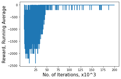
(a) Convergence of tabular importance sampling Q-learning algorithm ImRE.

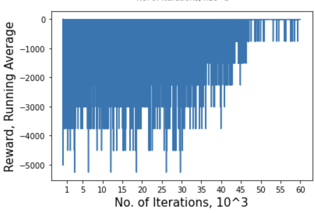
(b) Convergence of linear function approximation importance sampling algorithm ImFA.

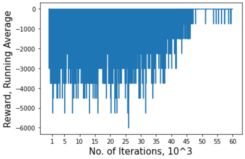
(c) Convergence of deep Q-learning importance sampling algorithm ImDQL.

Figure 2: Convergence of our proposed importance-sampling based rare events adaptive algorithms.

VII Simulations

In this section, we provide numerical evaluation for our algorithms ImRE, ImFA, and ImDQL, validating, and going beyond the results in Section IV. In particular, we show that we have solved the main research challenges identified in Section I. We show that our failure-adaptive importance sampling based algorithms ImRE, ImFA and ImDQL converged to optimality. We also show that they were able to learn a policy which mitigates the high cost of server failures, unlike the baselines in which importance sampling or backups were not used, given a tradeoff of incurring a higher average cost due to backup storage and migration during normal states. We perform our experiments with the help of real world traces.

We compare our proposed simulator algorithms (ImRE, ImDQL) with the following baselines. We will compare by applying the converged policy of each algorithm in an online scenario where the rare events occur at their true rate.

Q Learning with No Importance-Sampling (NIS): This simulator is a traditional Q-learning service migration algorithm in which there is no importance sampling of rare events. Rare events are still simulated, but at their true rate, and backups are used as a possible action.

Q Learning without Backups as an Action (WBA): This simulator is a Q-learning service migration algorithm in which there is no importance sampling of rare events and backups are not used as possible actions. Rare events are still simulated, at their true rate.

Q Learning without Rare Events Sampled (RES): This simulator is a Q-learning service migration algorithm under the “normal scenario”, in which rare events are not considered (not modelled) at all, during training. Likewise, backups are not considered as a possible action.

Each of these baselines may be trained with tabular or deep Q-learning, depending on the size of the state and action space. Comparing with NIS allows us to see the impact of not having importance sampling of rare events, unlike our algorithms ImRE and ImDQL. Comparing with WBA allows us to view the impact of not having backups. Finally, comparing with RES allows us to see the impact of not considering rare events at all.

Parameter settings: We run our experiments under the following settings, for both the 3 and 9 access point scenarios. The ns-3 network simulator [48] simulates realistic network conditions involving dynamic channels. We use it to obtain realistic latency (delay) costs across different user-server location pairs. The latencies obtained from this simulation are from the range (2,10), and are dependent on how far the different access points are from each other. As the migration cost is also a function of the distance between access points, we set the migration cost $m_{ij}$ to be $d^{comm}_{i,j}+\epsilon$, where $\epsilon\in(-0.5,0.5)$. We let the user be highly mobile across coverage areas. In particular, for the 3 access point case we set the mobility patterns to follow the probability distribution $[0.5,0.5,0],[0.15,0.1,0.75],[0.2,0.4,0.4]$. The natural failure rate is set to be $0.01$.

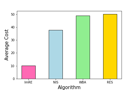
(a) Comparison of average cost.

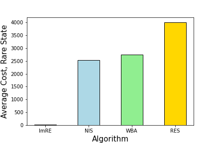
(b) Comparison of average cost at rare state, when failure occurs.

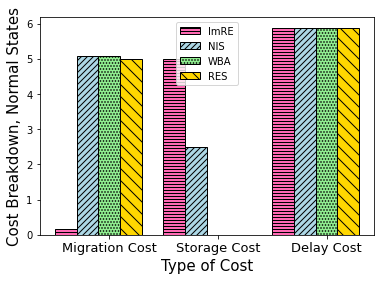
(c) Comparison of the average cost breakdown, at normal states.

Figure 3: Comparison of our tablular algorithm ImRE, with baselines NIS, WBA and RES, in an online scenario, in which backups are only placed at a single location.

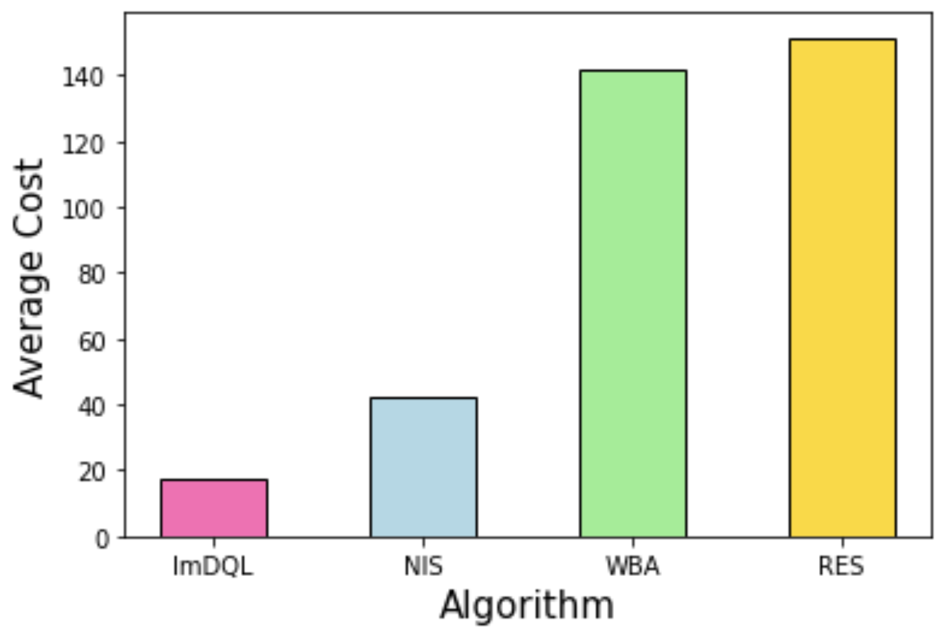
(a) Comparison of average cost.

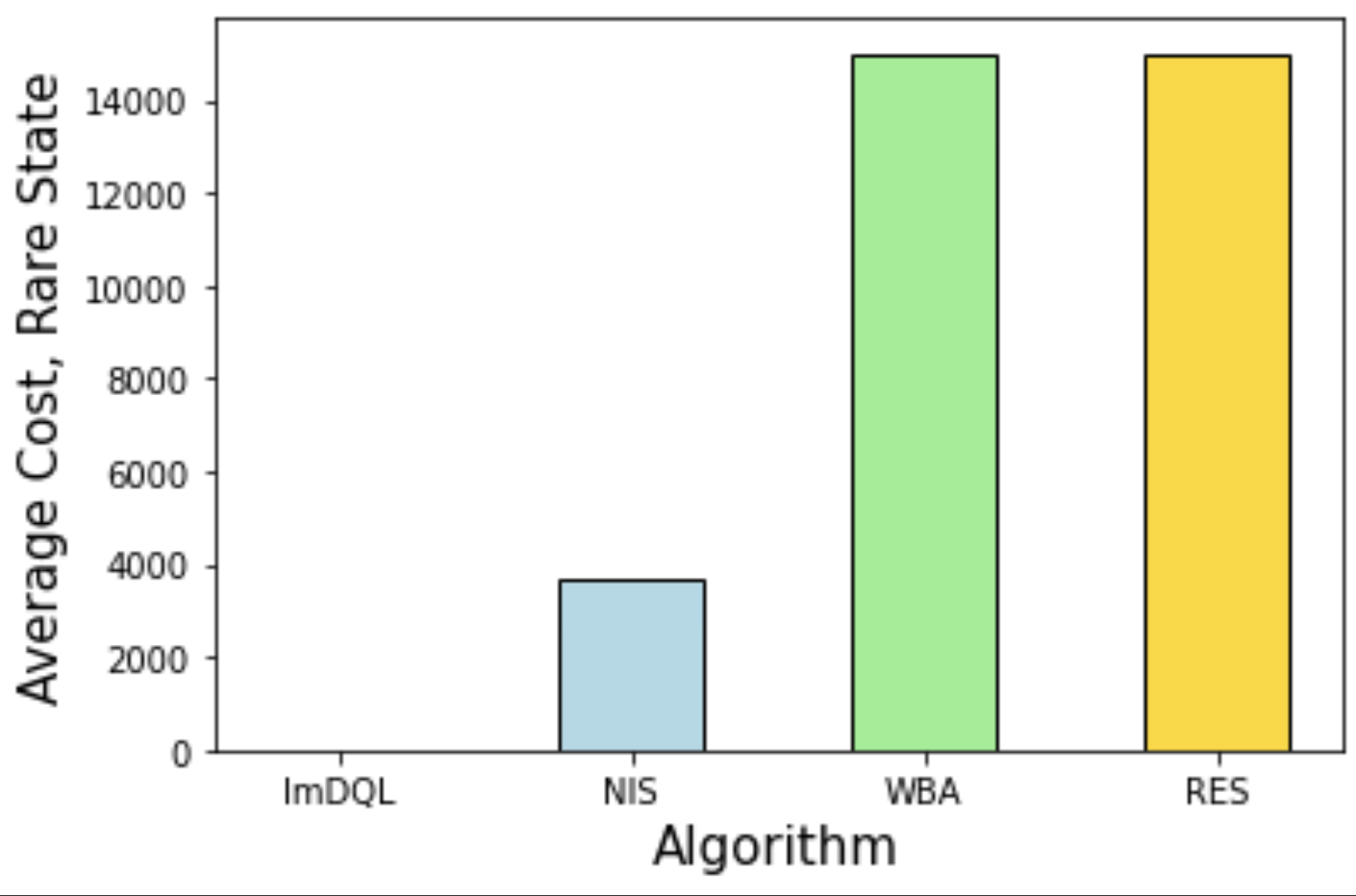
(b) Comparison of average cost at rare state, when failure occurs.

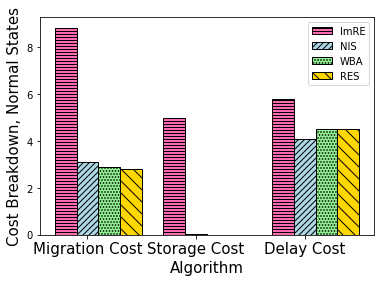
(c) Comparison of the average cost breakdown, at normal states.

Figure 4: Comparison of our deep Q-learning algorithm ImDQL, with baselines NIS, WBA and RES, in an online scenario, where backups are placed and migrated across multiple locations.

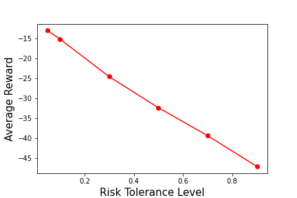
(a) Average reward.

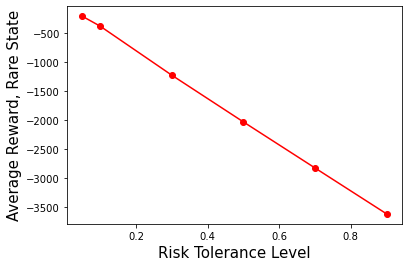
(b) Average reward at rare state, when failure occurs.

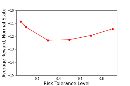
(c) Average reward at normal state.

Figure 5: How the input of different risk tolerance levels in Algorithm RiTA impacts the reward.

Convergence of ImRE, ImFA and ImDQL: Figure 2 illustrates how the algorithms we proposed in Section IV and V converged to the optimal reward. Firstly, Fig. 2a) illustrates how the importance sampling based tabular Q-learning algorithm ImRE (Algorithm 1) converges to the optimal reward. Here, we consider the case in which there are 3 access points, and set the cost of server failures to be -4000. The high cost represents the cost the user experiences when it is no longer able to get its task computed, which may have an impact on the safe and smooth functioning of the latency sensitive edge computing application. The learning rate used is $0.05$. Our algorithm is able to learn the optimal actions through importance sampling, as we have proved in Theorem 1, and enables the user to avoid the large cost incurred by server failures. In Fig. 2b), we illustrate that the function approximation version of our algorithm (ImFA, Algorithm 3) converges to the optimal reward for the 9 access point case, with a failure cost of -15000. The learning rate used is $\alpha=0.005$. The feature vector $\phi$ used is the identity matrix, indicating that the algorithm works without requiring further information for the feature vector. As seen in Fig. 2b), our algorithm is able to avoid the large cost incurred by server failures. For instance, at state $0$, the converged Q-values at action 89 ($l_{s}=9,b_{u}=\text{no backup}$) is $-75.207$, the converged Q-values at action 88 ($l_{s}=9,b_{u}=9$) is $-81.167$, while the converged Q-values at action 82 ($l_{s}=9,b_{u}=4$) is $-15.086$. This indicates that both not having a backup, and placing the backup at the same location as the main service is not recommended. In Fig. 2c), we show the convergence of ImDQL, the deep Q-learning version of our importance sampling algorithm. The neural network we use has the structure $[24,48,24]$, and a learning rate of $\alpha=0.1$ is used. In this scenario with 9 access points, there are 360 states and 90 actions. Here, we also show that our algorithm is able to learn to avoid the large cost incurred by server failures.

Backups at one location: Next, in Fig. 3 we illustrate how our tabular algorithm ImRE performs in comparison to the tabular baselines NIS, WBA and RES. We first study the simpler scenario in which there are storage constraints at some locations, and backups are only placed at one fixed access point. As mentioned earlier, all baselines are Q-learning algorithms with no importance sampling. NIS has backups as a possible action, while both WBA and RES have no backups as a choice of action involved. NIS and WBA do involve rare events - which occur at their true rate $p(s^{\prime}|s,a)$, while RES does not take into account rare events at all. The algorithms are compared by applying the algorithm’s converged policy in an online scenario in which rare events occur at their true rate $p(s^{\prime}|s,a)$, and obtaining the cost incurred. In Fig. 3a), we plot the average cost experienced across all timeslots (regardless of whether a rare event occurs) in the online scenario. Next, we plot the average cost experienced at rare states (Fig. 3b), and the average cost experienced at normal states (Fig. 3c). It can be seen that our importance sampling algorithm ImRE gives a lower average cost, and lower average costs at rare states, in the online scenario. This is because, the importance sampling algorithm sufficiently samples the rare events to learn an optimal policy. Our results show that it is optimal to place backups, and to place the main service at locations different from where the backup is. This allows users to offload their jobs at another location when the server at which their service was migrated to fails. Our results show that RES results in the highest cost during rare events, because rare events are not sampled at all during the simulator training, and backups are not a possible action. In Fig. 3c), we show how the average normal state cost breakdown differs across our algorithm and the baselines. It can be seen that the delay cost at normal states does not vary too much. The differences in migration cost occur because the baselines only manage to learn a uniform or random policy, and thus frequent migrations occur. For our algorithm, it manages to learn a policy in which frequent migrations do not occur. Finally, our algorithm incurs a higher storage than the baselines, which is a trade-off to help avoid the high failure costs during rare states.

Backups across multiple access points: Next, we study the more complicated scenario where there are less storage constraints across the system and backups are allowed to be placed and migrated across multiple access points. This incurs an additional cost of migration of backups. For the 9 access points scenario, we compare our deep Q-learning algorithm ImDQL with deep Q-learning versions of the baselines NIS, WBA and RES in Fig. 4. As we can see, our algorithm ImDQL results in a lower average cost, and a much lower average cost at rare states. It incurs a trade-off in the form of a higher average cost at normal states, resulting from the backup storage cost and backup migration cost. Our algorithm attains a much lower cost at rare states through the placement of backups and the use of importance sampling of rare events. The baseline NIS gives a higher cost than our algorithm because it does not perform importance sampling of rare events, and therefore does not help the learner train an optimal policy in light of rare events. It gives a lower cost than the algorithms WBA and RES as it allows for backups as a possible action.

Catering to varying risk tolerances: We study the impact of our algorithm RiTA (Algorithm 5) which caters to a variety of users with different risk tolerances, on the 3 AP scenario where backups are placed at a fixed location. Given the risk tolerance level of a user $\zeta$, with probability $\zeta$ RiTA will select an action according to the converged policy of the baseline RES (risk taking component), and with probability $1-\zeta$, RiTA will select an action according to the converged policy of our algorithm ImRE (risk adverse component). In Fig. 5 we present how the risk tolerance level $\zeta$ has an impact on the overall average reward, the reward at rare states when failure occurs, and the reward at normal states when there is no failure. It can be seen that the higher the risk tolerance, the higher the cost experienced at rare states (as it is less likely backups were placed), and hence the higher the average cost. During normal states, the cost difference is low. As the risk tolerance level $\zeta$ decreases, the cost first increases due to the increase in storage of backups (resulting from being increasingly risk adverse). After $\zeta=0.3$, the cost decreases. This is because the risk tolerant component (the baseline RES) only manages to learn a uniform or random policy, and therefore frequent migrations occur. As $\zeta$ decreases, the weightage given to the risk adverse component (our algorithm ImRE) increases. While ImRE incurs a higher storage cost than RES, it manages to learn a policy in which frequent migrations do not occur, hence decreasing the normal state cost (increasing the normal state reward).

VIII Conclusion

In edge computing, server failures may spontaneously occur, which complicates resource allocation and service migration. While failures are considered as rare events, they have an impact on the smooth and safe functioning of edge computing’s latency sensitive applications. As these failures occur at a low probability, it is difficult to jointly plan or learn an optimal service migration solution for both the typical and rare event scenarios. Therefore, we introduce a rare events adaptive resilience framework named FIRE, using the placement of backups and importance sampling based reinforcement learning which alters the sampling rate of rare events in order to learn an optimal policy. We prove the boundedness and convergence to optimality of our proposed tabular Q-learning algorithm ImRE. To speed up convergence we propose an eligibility traces version (ETAA), and prove that it is bounded. To handle large and combinatorial state and action spaces common in real-world networks, we propose a linear function approximation (ImFA) and a deep Q-learning (ImDQL) version of our algorithm. Furthermore, we propose a decision making algorithm (RiTA) which caters to heterogeneous risk tolerances across users.Finally, we use trace driven experiments to show that our algorithms convergence to optimality, and are resilient towards server failures unlike vanilla Q-learning, subject to a trade-off in terms of a potential higher normal state cost.

For future work, we will apply our framework to the multi-user scenario in service migration, while considering the computing delay users cause to others. Our framework can also be modified and extended to other resource allocation problems pertaining rare events with sizeable consequences in communication and networking.

References

- [1] Y. Mao, C. You, J. Zhang, K. Huang, and K. B. Letaief, “A survey on mobile edge computing: The communication perspective,” IEEE Communications Surveys & Tutorials, vol. 19, no. 4, pp. 2322–2358, 2017.
- [2] P. Mach and Z. Becvar, “Mobile edge computing: A survey on architecture and computation offloading,” IEEE Communications Surveys Tutorials, vol. 19, no. 3, pp. 1628–1656, 2017.
- [3] Y. C. Hu, M. Patel, D. Sabella, N. Sprecher, and V. Young, “Mobile edge computing—a key technology towards 5g,” ETSI white paper, vol. 11, no. 11, pp. 1–16, 2015.
- [4] Y. Mao, J. Zhang, and K. B. Letaief, “Dynamic computation offloading for mobile-edge computing with energy harvesting devices,” IEEE Journal on Selected Areas in Communications, vol. 34, no. 12, pp. 3590–3605, 2016.
- [5] X. Chen, L. Jiao, W. Li, and X. Fu, “Efficient multi-user computation offloading for mobile-edge cloud computing,” IEEE/ACM Transactions on Networking, vol. 24, no. 5, pp. 2795–2808, 2015.
- [6] T. Q. Dinh, J. Tang, Q. D. La, and T. Q. Quek, “Offloading in mobile edge computing: Task allocation and computational frequency scaling,” IEEE Transactions on Communications, vol. 65, no. 8, pp. 3571–3584, 2017.
- [7] L. Li, M. Siew, and T. Q. Quek, “Learning-based pricing for privacy-preserving job offloading in mobile edge computing,” in ICASSP 2019 - 2019 IEEE International Conference on Acoustics, Speech and Signal Processing (ICASSP), 2019, pp. 4784–4788.
- [8] S. Wang, R. Urgaonkar, M. Zafer, T. He, K. Chan, and K. K. Leung, “Dynamic service migration in mobile edge computing based on markov decision process,” IEEE/ACM Transactions on Networking, vol. 27, no. 3, pp. 1272–1288, 2019.
- [9] T. Ouyang, Z. Zhou, and X. Chen, “Follow me at the edge: Mobility-aware dynamic service placement for mobile edge computing,” IEEE Journal on Selected Areas in Communications, vol. 36, no. 10, pp. 2333–2345, 2018.
- [10] S. Wang, J. Xu, N. Zhang, and Y. Liu, “A survey on service migration in mobile edge computing,” IEEE Access, vol. 6, pp. 23 511–23 528, 2018.
- [11] S. Wang, Y. Guo, N. Zhang, P. Yang, A. Zhou, and X. Shen, “Delay-aware microservice coordination in mobile edge computing: A reinforcement learning approach,” IEEE Transactions on Mobile Computing, vol. 20, no. 3, pp. 939–951, 2019.
- [12] B. Gao, Z. Zhou, F. Liu, F. Xu, and B. Li, “An online framework for joint network selection and service placement in mobile edge computing,” IEEE Transactions on Mobile Computing, pp. 1–1, 2021.
- [13] T. Ouyang, R. Li, X. Chen, Z. Zhou, and X. Tang, “Adaptive user-managed service placement for mobile edge computing: An online learning approach,” in IEEE INFOCOM 2019-IEEE conference on computer communications. IEEE, 2019, pp. 1468–1476.
- [14] M. Siew, K. Guo, D. Cai, L. Li, and T. Q. Quek, “Let’s share vms: Optimal placement and pricing across base stations in mec systems,” in IEEE INFOCOM 2021-IEEE Conference on Computer Communications. IEEE, 2021, pp. 1–10.
- [15] T. Kim, S. D. Sathyanarayana, S. Chen, Y. Im, X. Zhang, S. Ha, and C. Joe-Wong, “Modems: Optimizing edge computing migrations for user mobility,” in IEEE INFOCOM 2022-IEEE Conference on Computer Communications. IEEE, 2022, pp. 1159–1168.
- [16] L. Ponemon, “Cost of data center outages,” Data Center Performance Benchmark Serie, 2016.
- [17] A. Aral and I. Brandić, “Learning spatiotemporal failure dependencies for resilient edge computing services,” IEEE Transactions on Parallel and Distributed Systems, vol. 32, no. 7, pp. 1578–1590, 2020.
- [18] D. Zeng, L. Gu, S. Pan, J. Cai, and S. Guo, “Resource management at the network edge: A deep reinforcement learning approach,” IEEE Network, vol. 33, no. 3, pp. 26–33, 2019.
- [19] Z. Gao, Q. Jiao, K. Xiao, Q. Wang, Z. Mo, and Y. Yang, “Deep reinforcement learning based service migration strategy for edge computing,” in 2019 IEEE International Conference on Service-Oriented System Engineering (SOSE), 2019, pp. 116–1165.
- [20] J. Frank, S. Mannor, and D. Precup, “Reinforcement learning in the presence of rare events,” in Proceedings of the 25th international conference on Machine learning, 2008, pp. 336–343.
- [21] T. Taleb and A. Ksentini, “An analytical model for follow me cloud,” in 2013 IEEE Global Communications Conference (GLOBECOM), 2013, pp. 1291–1296.
- [22] A. Ksentini, T. Taleb, and M. Chen, “A markov decision process-based service migration procedure for follow me cloud,” in 2014 IEEE International Conference on Communications (ICC), 2014, pp. 1350–1354.
- [23] S. N. Shirazi, A. Gouglidis, A. Farshad, and D. Hutchison, “The extended cloud: Review and analysis of mobile edge computing and fog from a security and resilience perspective,” IEEE Journal on Selected Areas in Communications, vol. 35, no. 11, pp. 2586–2595, 2017.
- [24] C.-F. Liu, M. Bennis, M. Debbah, and H. V. Poor, “Dynamic task offloading and resource allocation for ultra-reliable low-latency edge computing,” IEEE Transactions on Communications, vol. 67, no. 6, pp. 4132–4150, 2019.
- [25] H. Huang and S. Guo, “Proactive failure recovery for nfv in distributed edge computing,” IEEE Communications Magazine, vol. 57, no. 5, pp. 131–137, 2019.
- [26] G. Yao, X. Li, Q. Ren, and R. Ruiz, “Failure-aware elastic cloud workflow scheduling,” IEEE Transactions on Services Computing, pp. 1–14, 2022.
- [27] Y. Liang, Z. Hu, and L. Yang, “A two-stage replica management mechanism for latency-aware applications in multi-access edge computing,” in 2021 IEEE Intl Conf on Parallel & Distributed Processing with Applications, Big Data & Cloud Computing, Sustainable Computing & Communications, Social Computing & Networking (ISPA/BDCloud/SocialCom/SustainCom). IEEE, 2021, pp. 453–459.
- [28] R. Zhang, F. R. Yu, J. Liu, T. Huang, and Y. Liu, “Deep reinforcement learning (drl)-based device-to-device (d2d) caching with blockchain and mobile edge computing,” IEEE Transactions on Wireless Communications, vol. 19, no. 10, pp. 6469–6485, 2020.
- [29] W. Du, Q. He, Y. Ji, C. Cai, and X. Zhao, “Optimal user migration upon server failures in edge computing environment,” in 2021 IEEE International Conference on Web Services (ICWS). IEEE, 2021, pp. 272–281.
- [30] A. Aral and I. Brandić, “Learning spatiotemporal failure dependencies for resilient edge computing services,” IEEE Transactions on Parallel and Distributed Systems, vol. 32, no. 7, pp. 1578–1590, 2021.
- [31] X. Chen, H. Zhang, C. Wu, S. Mao, Y. Ji, and M. Bennis, “Optimized computation offloading performance in virtual edge computing systems via deep reinforcement learning,” IEEE Internet of Things Journal, vol. 6, no. 3, pp. 4005–4018, 2018.
- [32] J. Wang, L. Zhao, J. Liu, and N. Kato, “Smart resource allocation for mobile edge computing: A deep reinforcement learning approach,” IEEE Transactions on emerging topics in computing, vol. 9, no. 3, pp. 1529–1541, 2019.
- [33] J. Zhang, X. Hu, Z. Ning, E. C.-H. Ngai, L. Zhou, J. Wei, J. Cheng, and B. Hu, “Energy-latency tradeoff for energy-aware offloading in mobile edge computing networks,” IEEE Internet of Things Journal, vol. 5, no. 4, pp. 2633–2645, 2017.
- [34] D. Precup, “Eligibility traces for off-policy policy evaluation,” Computer Science Department Faculty Publication Series, p. 80, 2000.
- [35] R. S. Sutton and A. G. Barto, Reinforcement learning: An introduction. MIT press, 2018.
- [36] U. Madhushani, B. Dey, N. E. Leonard, and A. Chakraborty, “Hamiltonian q-learning: Leveraging importance-sampling for data efficient rl,” arXiv preprint arXiv:2011.05927, 2020.
- [37] L. Ma, S. Yi, and Q. Li, “Efficient service handoff across edge servers via docker container migration,” in Proceedings of the Second ACM/IEEE Symposium on Edge Computing, 2017, pp. 1–13.
- [38] S. Wang, R. Urgaonkar, M. Zafer, T. He, K. Chan, and K. K. Leung, “Dynamic service migration in mobile edge computing based on markov decision process,” IEEE/ACM Transactions on Networking, vol. 27, no. 3, pp. 1272–1288, 2019.
- [39] J. A. Bucklew and J. Bucklew, Introduction to rare event simulation. Springer, 2004, vol. 5.
- [40] J. N. Tsitsiklis, “Asynchronous stochastic approximation and q-learning,” Machine learning, vol. 16, no. 3, pp. 185–202, 1994.
- [41] T. Jaakkola, M. Jordan, and S. Singh, “Convergence of stochastic iterative dynamic programming algorithms,” Advances in neural information processing systems, vol. 6, 1993.
- [42] C. J. C. H. Watkins, “Learning from delayed rewards,” 1989.
- [43] “Code for algorithm imdql.” [Online]. Available: https://github.com/ShikhSh/FIRE-A-failure-adaptive-RL-framework-for-Edge-Computing
- [44] V. Mnih, K. Kavukcuoglu, D. Silver, A. A. Rusu, J. Veness, M. G. Bellemare, A. Graves, M. Riedmiller, A. K. Fidjeland, G. Ostrovski et al., “Human-level control through deep reinforcement learning,” nature, vol. 518, no. 7540, pp. 529–533, 2015.
- [45] P. A. Apostolopoulos, E. E. Tsiropoulou, and S. Papavassiliou, “Risk-aware data offloading in multi-server multi-access edge computing environment,” IEEE/ACM Transactions on Networking, vol. 28, no. 3, pp. 1405–1418, 2020.
- [46] M. S. Munir, S. F. Abedin, N. H. Tran, Z. Han, E.-N. Huh, and C. S. Hong, “Risk-aware energy scheduling for edge computing with microgrid: A multi-agent deep reinforcement learning approach,” IEEE Transactions on Network and Service Management, vol. 18, no. 3, pp. 3476–3497, 2021.
- [47] H. Badri, T. Bahreini, D. Grosu, and K. Yang, “Risk-aware application placement in mobile edge computing systems: A learning-based optimization approach,” in 2020 IEEE International Conference on Edge Computing (EDGE), 2020, pp. 83–90.
- [48] “ns3 network simulator.” [Online]. Available: https://www.nsnam.org/