TESS spots a mini-neptune interior to a hot saturn in the TOI-2000 system

Abstract

Hot jupiters ($P<10\,\text{d},M>60\,\mathrm{M}_{\oplus}$) are almost always found alone around their stars, but four out of hundreds known have inner companion planets. These rare companions allow us to constrain the hot jupiter’s formation history by ruling out high-eccentricity tidal migration. Less is known about inner companions to hot Saturn-mass planets. We report here the discovery of the TOI-2000 system, which features a hot Saturn-mass planet with a smaller inner companion. The mini-neptune TOI-2000 b ($2.70$$\pm 0.15$$\,\mathrm{R}_{\oplus}$, $11.0$$\pm 2.4$$\,\mathrm{M}_{\oplus}$) is in a 3.10-day orbit, and the hot saturn TOI-2000 c ($8.14$${}_{-0.30}^{+0.31}$$\,\mathrm{R}_{\oplus}$, $81.7$${}_{-4.6}^{+4.7}$$\,\mathrm{M}_{\oplus}$) is in a 9.13-day orbit. Both planets transit their host star TOI-2000 (TIC 371188886, $V=10.98$, TESS magnitude $=10.36$), a metal-rich ($[\text{Fe}/\text{H}]=$ $0.439$${}_{-0.043}^{+0.041}$) G dwarf 174 pc away. TESS observed the two planets in sectors 9–11 and 36–38, and we followed up with ground-based photometry, spectroscopy, and speckle imaging. Radial velocities from CHIRON, FEROS, and HARPS allowed us to confirm both planets by direct mass measurement. In addition, we demonstrate constraining planetary and stellar parameters with MIST stellar evolutionary tracks through Hamiltonian Monte Carlo under the PyMC framework, achieving higher sampling efficiency and shorter run time compared to traditional Markov chain Monte Carlo. Having the brightest host star in the $V$ band among similar systems, TOI-2000 b and c are superb candidates for atmospheric characterization by the JWST, which can potentially distinguish whether they formed together or TOI-2000 c swept along material during migration to form TOI-2000 b.

1 Introduction

Hot gas giant planets ($P<10$ d, $M>$60\text{\,}\mathrm{\mathrm{M}}_{\mathrm{\oplus}}$$; also known as hot jupiters) are rarely observed with an inner companion planet (Huang et al., 2016; Hord et al., 2021). This relative scarcity is consistent with the hypothesis that high-eccentricity migration (HEM) may be responsible for the formation of many, if not most, hot gas giants (see Dawson & Johnson 2018 for a review). Under HEM, a hot gas giant first forms ‘cold’ at an orbital separation of several astronomical units and then enters into an orbit of high eccentricity by interacting with other planets in the system or another star (Rasio & Ford, 1996; Weidenschilling & Marzari, 1996; Wu & Murray, 2003). Later, tidal interaction with the host star dissipates the hot gas giant’s orbital energy and circularizes its orbit. This dynamically disruptive process would likely have eliminated any inner companions in the system (Mustill et al., 2015).

Two alternative mechanisms may explain how hot gas giants with inner companions formed. Under disc migration, tidal interactions with the protoplanetary disc move the initially cold gas giant to its present location (Lin et al. 1996; see Baruteau et al. 2014 for a review), sweeping material along its mean-motion resonances (MMRs) to form inner companions (Raymond et al., 2006). The other alternative has the giant planet forming in situ, near its present location (Lee et al., 2014; Batygin et al., 2016; Boley et al., 2016; Lee & Chiang, 2016; Poon et al., 2021). Thus, measuring the occurrence rate of inner companions may quantify the fraction of hot gas giants that formed under these two mechanisms as opposed to under HEM.

Until recently, efforts to measure the occurrence rate of hot gas giants’ inner companions were hampered by the lack of detections. Early studies looked for transit timing variations (TTVs) of known hot gas giants induced by possible companions near MMRs but found no significant TTVs of their targets (Steffen & Agol, 2005; Miller-Ricci et al., 2008a, b; Gibson et al., 2009). After the launch of Kepler, Latham et al. (2011) analysed 117 transiting multiplanet systems that have at least one hot planet candidate ($P<$10\text{\,}\mathrm{d}$$) and concluded that only $4^{+9}_{-2}$ per cent have giant planets bigger than Neptune, a rate considerably lower than the $31^{+4}_{-3}$ per cent of 405 hot planet candidates analysed in total that are bigger than Neptune. Steffen et al. (2012) additionally searched for TTV signals in Kepler light curves of hot jupiters and ruled out the existence of all but the least massive ($M\lesssim$1\text{\,}\mathrm{\mathrm{M}}_{\mathrm{\oplus}}$$) companions near MMRs. Using data from the full Kepler mission, Huang et al. (2016) found no inner companions to 45 hot jupiters in their sample, but found that half or more of 27 warm jupiters ($$10\text{\,}\mathrm{d}$\leq P<$200\text{\,}\mathrm{d}$$) searched had small coplanar nearby companions. More recently, Hord et al. (2021) found no additional transiting planets in the light curves of 184 confirmed hot jupiters from the first year of observations by the Transiting Exoplanet Survey Satellite (TESS; Ricker et al., 2015).

Nevertheless, Kepler and TESS have detected a handful of inner companions to hot gas giants. Out of the almost 500 transiting hot gas giants published in the literature, four are known to have inner companions: WASP-47 b (Becker et al., 2015; Vanderburg et al., 2017; Bryant & Bayliss, 2022; Hellier et al., 2012), Kepler-730 b (Zhu et al., 2018; Cañas et al., 2019), TOI-1130 c (Huang et al. 2020c; Korth et al. 2023) and WASP-132 b (Hord et al., 2022; Hellier et al., 2017). These exceptional planets may be important for understanding the formation of hot gas giant systems, so it is natural to ask if they share a formation history that is distinct from hot gas giants without inner companions. Currently, however, the sample of systems with companions is too small and relatively uncharacterized to answer that question.

Adding to this growing, but still small, family, we report the discovery of the TOI-2000 system, which hosts the smallest hot gas giant known to have an interior planet. We found the system through a systematic multi-planet search of the full-frame image (FFI) light curves of all hot gas giants observed by TESS during its two-year prime mission. We conducted a series of ground-based follow-up photometry, spectroscopy, and speckle imaging (Section 2). By constructing a joint model of transit light curves, radial velocities, and broadband photometry, we derive the planetary masses and other physical parameters of the TOI-2000 system and demonstrate a way to interpolate MIST stellar evolutionary tracks when using Hamiltonian Monte Carlo (HMC) for parameter fitting (Section 3). We then argue for the confirmation of the inner mini-neptune (TOI-2000 b) and the outer hot saturn (TOI-2000 c) by carefully considering and rejecting alternative explanations for the two planets’ signals (Section 4). Finally, we compare the two planets to those in similar planetary systems, point out they might show TTVs, and explore future observations that may constrain how they formed, ending with a note on why interpolating MIST tracks under HMC is generally preferred over traditional Markov chain Monte Carlo (Section 5).

2 Observations and Data Reduction

2.1 Photometry

We present space and ground-based photometry of TOI-2000 in this section. Table 1 summarizes the observations, and Figure 1 shows the light curves.

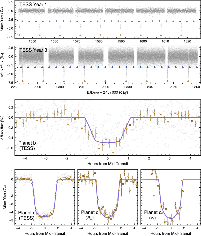
Figure 1: Light curves of TOI-2000. Top two rows: Detrended light curves from TESS years 1 and 3. Year 1 points are from the 30-min full-frame images, whilst year 3 points are binned to 2 min from the 20-s time series, which results in higher scatter per cadence but lower scatter at 30 min. The upright triangles indicate transits of planet b (blue) and planet c (orange). Bottom two rows: Phase-folded light curves zoomed in on the transits of planets b (third row) and c (last row). The purple line is the transit model, and the label in each panel indicates the passband of the limb darkening parameters. For the TESS light curves, the faint grey marks are observations both years, with year 3 observations binned to 30 min to be consistent with those from year 1. The orange marks of the TESS light curves are binned means (15-min bins for planet b and 10 min for planet c), with the error bars representing the standard error of the mean. The middle and right panels of the bottom row show planet c transit light curves from ground observations (ASTEP in the $R_{\mathrm{c}}$ band, LCOGT SSO in $z_{\mathrm{s}}$). For the ground observations, the orange marks are 12-min binned means weighted by inverse variance and the error bars are the standard error of the weighted mean.

Table 1: Summary of photometric observations.

Facility & Telescope	Date(s)	Planet	Transit	Transit(s)	No. Images	Exp. Time	Filter	Used in
	(UT)		Coverage	Detected?		(s)		Joint Model?
TESS camera 3	2019 Feb 28 – May 21	All	Full	Y	1612	1800	TESS	Y
TESS camera 3	2021 Mar 7 – May 26	All	Full	Y	111410	20	TESS	Y
LCOGT SSO 1 m	2021 Feb 10	c	Full	Y	129	30	$B$	N
LCOGT SSO 1 m	2021 Feb 10	c	Full	Y	128	30	$z_{\mathrm{s}}$	Y
PEST	2021 Apr 24	c	Full	Y	168	60	$B$	N
PEST	2021 Apr 24	c	Full	Y	167	60	$I_{\mathrm{c}}$	N
ASTEP 0.4 m	2021 May 3	c	Full	Y	427	70	$R_{\mathrm{c}}$	Y
LCOGT SSO 1 m	2021 Jan 18	b	Full	N	467	20	$i^{\prime}$	N
LCOGT CTIO 1 m	2021 Feb 6	b	Full	N	515	20	$i^{\prime}$	N
LCOGT SAAO 1 m	2021 Apr 27	b	Ingress	N	190	15	$i^{\prime}$	N
LCOGT CTIO 1 m	2021 Dec 16	b	Full	N	305	15	$i^{\prime}$	N
LCOGT SAAO 1 m	2022 Jan 7	b	Full	N	324	15	$i^{\prime}$	N
LCOGT CTIO 0.4 m	2022 May 16	b	Full	N	133	100	$i^{\prime}$	N

Table 2: TESS light curve of TOI-2000 from year 1 at 30-minute cadence. (The entire table is available electronically in machine-readable format.)

$\mathrm{BJD}_{\text{TDB}}$	Flux	Detrended Flux
${}-$2\,457\,000$$	(normalized)	(normalized)
1543.783216	1.00716	1.00027
1543.804029	1.00661	0.99986
1543.824903	1.00622	0.99960
1543.845716	1.00698	1.00049
1543.866530	1.00644	1.00008
…	…	…

Table 3: TESS light curve of TOI-2000 from year 3 at 20-second cadence. (The entire table is available electronically in machine-readable format.)

$\mathrm{BJD}_{\text{TDB}}$	Detrended Flux	Uncertainty
${}-$2\,457\,000$$	(normalized)
2281.876943	0.9993	0.0027
2281.877174	0.9989	0.0027
2281.877406	0.9986	0.0027
2281.877637	0.9989	0.0027
2281.877869	1.0034	0.0027
…	…	…

Table 4: LCOGT (Siding Spring Observatory) light curve of TOI-2000. (The entire table is available electronically in machine-readable format.)

$\mathrm{BJD}_{\text{TDB}}$	Flux	Unc.	Width	Sky	Airmass	Exp. Time	Filter
${}-$2\,457\,000$$	(normalized)		(pixel)	(count/pixel)		(s)
2255.980346	0.9950	0.0011	15.323563	19.373182	1.392324	29.976	$B$
2255.981878	1.0028	0.0010	11.535994	15.302150	1.387933	29.976	$B$
2255.983397	1.0044	0.0010	12.790320	15.547044	1.383667	29.972	$B$
2255.984914	1.0060	0.0010	12.572493	15.866800	1.379476	29.972	$B$
2255.986431	1.0042	0.0010	11.599984	15.431446	1.375335	29.972	$B$
…	…	…	…	…	…	…	…

Table 5: PEST light curve of TOI-2000. (The entire table is available electronically in machine-readable format.)

$\mathrm{BJD}_{\text{TDB}}$	Flux	Unc.	Airmass	Filter
${}-$2\,457\,000$$	(normalized)
2328.9512276	1.0023	0.0047	1.2571	$B$
2328.9527553	1.0050	0.0047	1.2556	$B$
2328.9542715	1.0014	0.0047	1.2541	$B$
2328.9557993	1.0022	0.0046	1.2527	$B$
2328.9573271	1.0000	0.0046	1.2513	$B$
…	…	…	…	…

Table 6: ASTEP light curve of TOI-2000. (The entire table is available electronically in machine-readable format.)

$\mathrm{BJD}_{\text{TDB}}$	Flux	Unc.	Airmass	Sky
${}-$2\,457\,000$$	(normalized)			(count)
2338.006101	0.9992	0.0012	1.017	201
2338.007462	1.0007	0.0012	1.017	203
2338.009370	0.9985	0.0012	1.017	203
2338.010466	1.0016	0.0012	1.018	203
2338.011563	0.9982	0.0012	1.018	209
…	…	…	…	…

2.1.1 TESS Photometry

TESS observed TOI-2000 in camera 3 during years 1 and 3 of its mission. In year 1, TOI-2000 was observed in the FFIs at a 30-min cadence during sectors 9–11 (ut 2019 February 28 – May 21). The MIT Quick Look Pipeline (qlp; Huang et al., 2020a, b) detected the outer planet as a 9.13-day transit signal with a depth of 0.43 per cent at a signal–to–pink noise ratio (S/PN) of 30.62, and it was released as TESS Object of Interest (TOI) 2000.01, having passed all vetting criteria (Guerrero et al., 2021). We renamed TOI-2000.01 to TOI-2000 c following its confirmation in this paper.

After removing the points where TOI-2000 c was in transit, we detected the 3.10-day signal of the inner planet with a depth of $474_{-42}^{+39}$ parts per million (ppm) at a S/PN of $10.56$ through a boxed least-squares (BLS) search (Kovács et al., 2002) of the qlp light curve. This search was part of a systematic effort to identify possible inner companions to all confirmed and candidate hot gas giants observed by TESS during its two-year prime mission. Later in year 3, TOI-2000 was selected by the TESS mission for 20-s fast cadence observation during sectors 36–38 in camera 3 (ut 2021 March 7 – May 26). Subsequently, the TESS Science Processing Operations Center pipeline (SPOC pipeline; Jenkins et al., 2016, 2010, 2020; Jenkins, 2002) independently detected the signal of the inner planet in a search of sectors 1–39 in 2021 August with a multi-event statistic of $9.5$ and a signal-to-noise ratio (S/N) of $10.3$. The transit signature of the inner planet passed all the diagnostic tests (Twicken et al., 2018; Li et al., 2019) and the TESS Science Office issued an alert on 2022 March 24 for the planet as TOI-2000.02, which we renamed to TOI-2000 b in this paper. In addition, the difference image centroiding of the SPOC pipeline located the source of the transit signatures to within $$$\pm$$$ and $$$\pm$$$ of TOI-2000 for planets c and b, respectively.

To produce the year 1 light curve, we used the SPOC-calibrated FFIs obtained from the TESSCut service (Brasseur et al., 2019). We performed photometry with a series of 20 different apertures and corrected these light curves for dilution from the light of other nearby stars. To make this correction, we first determined the fraction of light from other stars in each aperture by simulating the TESS image with and without contaminating sources using the location and brightness of nearby stars from the TESS Input Catalog (TIC; Stassun et al., 2018b, 2019) and the measured instrument pixel response function, which we determined at the position of the star on the detector using bilinear interpolation. We then subtracted the contaminating flux and re-normalized the resulting light curves.

After correcting for dilution in the year 1 light curves of each aperture, we removed instrumental systematics from the light curves by decorrelating the light curves against the mean and standard deviation of the spacecraft pointing quaternion time series within each exposure (processed similarly to Vanderburg et al., 2019) and the TESS 2-min cadence pre-search data conditioning (PDC) band 3 (fast-timescale) cotrending basis vectors (CBVs) binned to 30 min. We modeled low-frequency light curve variability with a B-spline and excluded the points during transits from the systematics correction. We performed the fit using least squares while iteratively identifying and removing outliers. After correcting systematics in each aperture, we selected the aperture in each sector that minimized the scatter in the light curve. The best apertures chosen for the final light curve were all roughly circular and included a total of 14, 8, and 9 pixels in sectors 9, 10, and 11, respectively. The processed light curve with and without detrending by B-spline can be found in Table 2.

For the year 3 TESS data, we used the SPOC pipeline’s simple aperture photometry flux (SAP_FLUX) from the 20-s target pixel file and performed our own systematics correction using a process similar to the 30-min cadence year 1 data. As before, we exclude points during transits from the systematics correction and decorrelated against the spacecraft pointing quaternion time series and the 20-s PDC band 3 CBVs while modelling the low-frequency variability as a B-spline. We then corrected for the contaminating flux from nearby stars using the value in the target pixel file’s CROWDSAP header. The processed light curve can be found in Table 3.

To look for additional planets in the TESS light curve, we performed BLS searches after masking out the portions containing the two known planets’ transits, following procedures described by Vanderburg et al. (2016). No additional transiting planets were found above our detection threshold ($\mathrm{S}/\mathrm{N}>9$).

2.1.2 Ground-based photometry of TOI-2000 c

We observed multiple transits of TOI-2000 c using ground-based seeing-limited photometry to confirm that the transit signal originated from the expected host star. We observed three full transits with high S/N at different facilities and in various passbands during the first half of 2021. We detail the three full-transit observations below. The lower right panel in Figure 1 shows the phase-folded light curve of all ground-based observations in bins weighted by inverse variance.

The Las Cumbres Observatory Global Telescope (LCOGT; Brown et al., 2013) 1-m network node at Siding Spring Observatory, Australia observed a full transit of TOI-2000 c on ut 2021 February 10 in the $B$ and $z_{\mathrm{s}}$ bands. Differential photometric data were extracted using AstroImageJ (Collins et al., 2017) and circular photometric apertures with radii $5.\mathrm{″}8$ and $6.\mathrm{″}2$. The apertures exclude flux from all nearby Gaia EDR3 stars that are bright enough to cause the event in the TESS aperture. The event arrived on time. The light curves in both filters can be found in Table 4.

The Perth Exoplanet Survey Telescope (PEST, a $12^{\prime\prime}$ Meade LX200 SCT Schmidt–Cassegrain telescope in Perth, Australia) observed a full transit of TOI-2000 c in alternating $B$ and $I_{\mathrm{c}}$ bands at $60\text{\,}\mathrm{s}$ cadence on ut 2021 April 24. The photometric apertures were uncontaminated and sized $9.\mathrm{″}2$ and $7.\mathrm{″}8$, respectively. The transit was detected on time in the $I_{\mathrm{c}}$ band but was more marginal in the $B$ band. Detrending by airmass improved the $B$ band signal. Table 5 contains the light curve in both filters.

The 0.4-m telescope of the Antarctica Search for Transiting Exoplanets (ASTEP; Guillot et al., 2015) programme at Dome C, Antarctica observed a full transit of TOI-2000 c on ut 2021 May 3 with an uncontaminated $9.\mathrm{″}3$ aperture in the $R_{\mathrm{c}}$ band. The event arrived on time. The light curve, extracted through procedures described by Mékarnia et al. (2016), can be found in Table 6.

2.1.3 Ground-based photometry of TOI-2000 b

We observed TOI-2000 using LCOGT telescopes on six nights in 2021 and 2022. The transit of TOI-2000 b is too shallow ($\approx 470\,\text{ppm}$) to detect on target in standard ground-based observations, so instead the goal of our observations was to rule out that the periodic transit signal of TOI-2000 b detected in TESS light curves actually originated from nearby sources in the sky. As detailed in Table 1, we mostly used the 1-m telescopes on the LCOGT sites at Siding Spring Observatory in Australia, Cerro Tololo Inter-American Observatory in Chile, and South African Astronomical Observatory in South Africa. Using the observations on ut 2021 February 6 at Cerro Tololo Inter-American Observatory, Chile, which covered nearly 6 hours before the transit ingress, the full transit ingress, and more than 70 per cent of the transit window, we were able to rule out that the transit event occurred on all nearby Gaia EDR3 targets within $2^{\prime}$, except for a $\Delta\mathrm{mag}=8.7$ (TESS band) neighbour $5.\mathrm{″}3$ north of the target, TIC 845089585.

As expected, we could not confidently detect the shallow transit signal due to TOI-2000 b during those observations. Nevertheless, the ground-based photometry rules out virtually all potential nearby sources of contamination, which allows us to rule out the false-positive scenario due to resolved nearby eclipsing binaries in Section 4.3.

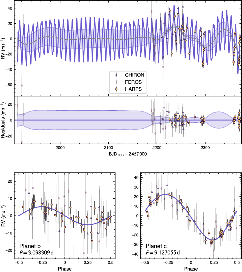
Figure 2: RV measurements of TOI-2000. The shapes and colours of each mark indicate which spectrograph it corresponds to, and its error bar is the quadrature sum of uncertainty and an instrumental jitter term (Section 3.3). Solid purple lines represent the best-fitting RV model. Top: The best-fitting RV and Gaussian process (GP) model. The dashed grey line represents the inferred GP model of residuals in excess of known planet-induced variations. The purple-shaded interval represent the $1\sigma$ uncertainty of the GP model. Middle: Residual of the RV measurements with respect to the best-fitting RV and GP model. Bottom left: Phase-folded RV variations due to planet b only. Bottom right: Phase-folded RV variations due to planet c only.

Table 7: Summary of spectroscopic observations.

Instrument	Date(s)	No. Spectra	Resolution	Wavelengths	S/N	Jitter		$\gamma$
	(UT)		$(\lambda/\Delta\lambda/1000)$	(nm)	(at $500\text{\,}\mathrm{nm}$)	($\mathrm{m}\text{\,}{\mathrm{s}}^{-1}$)		($\mathrm{m}\text{\,}{\mathrm{s}}^{-1}$)
CHIRON	2020 Dec 24 – 2021 Feb 10	15	80	410–870	70	$3.4$	${}_{-2.3}^{+3.2}$	$6647.7$	${}_{-12.8}^{+8.8}$
FEROS	2020 Mar 3 – 2021 Jan 6	14	48	350–920	56–97	$14.0$	${}_{-3.3}^{+4.5}$	$8116$	${}_{-14}^{+11}$
HARPS	2021 Jan 12 – Jun 7	41	115	378–691	27.9–56.4	$3.14$	${}_{-0.78}^{+0.82}$	$8118.1$	${}_{-12.2}^{+8.2}$

Table 8: Radial velocity measurements of TOI-2000. The RVs from FEROS and HARPS are measured relative to the Solar System barycentre. (The entire table is available electronically in machine-readable format.)

$\mathrm{BJD}_{\text{TDB}}$	RV	Uncertainty	Instrument
${}-$2\,457\,000$$	($\mathrm{m}\text{\,}{\mathrm{s}}^{-1}$)	($\mathrm{m}\text{\,}{\mathrm{s}}^{-1}$)
$2207.81850$	$6671.1$	$8.2$	CHIRON
$2210.82757$	$6650.5$	$9.6$	CHIRON
$2212.80571$	$6624.8$	$8.7$	CHIRON
…	…	…	…
$1911.72374$	$8106.2$	$6.3$	FEROS
$1920.62204$	$8056.3$	$6.1$	FEROS
$1924.57801$	$8136.1$	$6.6$	FEROS
…	…	…	…
$2226.762805$	$8155.81$	$2.10$	HARPS
$2230.798279$	$8099.73$	$2.46$	HARPS
$2236.721230$	$8148.55$	$3.74$	HARPS
…	…	…	…

2.2 Spectroscopy

We observed TOI-2000 with the CHIRON, FEROS, and HARPS spectrographs, and the details are summarized in Table 7. Table 8 lists all the radial velocity (RV) measurements and their uncertainties, which are also shown in Figure 2.

We obtained 15 spectra of TOI-2000 with the CHIRON spectrograph (Tokovinin et al., 2013) on the $1.5\text{\,}\mathrm{m}$ SMARTS telescope located at Cerro Tololo Inter-American Observatory, Chile. CHIRON is a high-resolution echelle spectrograph, fed via a fibre bundle, with a spectral resolving power of $\lambda/\Delta\lambda\equiv R\approx$80\,000$$ from $41008700\text{\,}\mathrm{\AA}$ for slicer mode observations. The spectra were extracted by the standard CHIRON pipeline (Paredes et al., 2021). The RVs were derived for each spectrum by cross-correlating against a median-combined template spectrum. The template spectrum was a median combination of all CHIRON spectra, each shifted to rest after an approximate velocity measurement via cross correlation against a synthetic template. The measured velocity of each spectrum is that of the mean velocity from each spectral order, weighted by their cross correlation function heights. The velocity uncertainties were estimated from the scatter of the per-order velocities. We find a mean internal uncertainty of $9\text{\,}\mathrm{m}\text{\,}{\mathrm{s}}^{-1}$ and S/N $\approx 70$ per spectral resolution element.

We acquired 14 spectra of TOI-2000 at $R\approx$48\,000$$ with the FEROS spectrograph (Kaufer et al., 1999) mounted on the MPG/ESO 2.2-m telescope at La Silla observatory, Chile between ut 2020 March 3 and 2021 January 6. Most of the spectra had an exposure time of $600\text{\,}\mathrm{s}$, but two had an exposure time of $900\text{\,}\mathrm{s}$ due to poor weather. The mean and median S/N per spectral resolution element were 82.4 and 83, respectively, ranging 56–97 in total. The instrumental drift was calibrated by simultaneously observing a fibre illuminated with a ThAr+Ne lamp. The data were processed with the CERES suite of echelle pipelines (Brahm et al., 2017), which produced RVs and bisector spans in addition to reduced spectra.

We acquired 41 spectra of TOI-2000 at $R\approx$115\,000$$ with the High Accuracy Radial velocity Planet Searcher spectrograph (HARPS; Mayor et al., 2003) between ut 2021 January 12 and June 7. HARPS is fibre-fed by the Cassegrain focus of the 3.6-m telescope at La Silla Observatory, Chile. The spectra were taken with exposure times between $9001800\text{\,}\mathrm{s}$ in high-accuracy mode (HAM), resulting in S/N of 27.1–56.5 at spectral order 60 for individual spectra, except for a poor quality one at $\mathrm{BJD}_{\text{TDB}}$ $2\,459\,282.76$, which we excluded from the joint model (Section 3.3). The spectra were reduced with the standard Data Reduction Software (DRS; Pepe et al., 2002; Baranne et al., 1996), using a K0 template to correct the flux balance over spectral orders before applying a G2 binary cross-correlation function (CCF) mask. Such colour correction allowed us to minimize the impact of the CCF mask mismatch between the observed spectral type and the CCF binary mask. The K0 flux template was selected as the closest one to a G5–G6 star like TOI-2000, and the G2 binary mask was selected to minimize photon noise uncertainty.

2.3 Speckle imaging

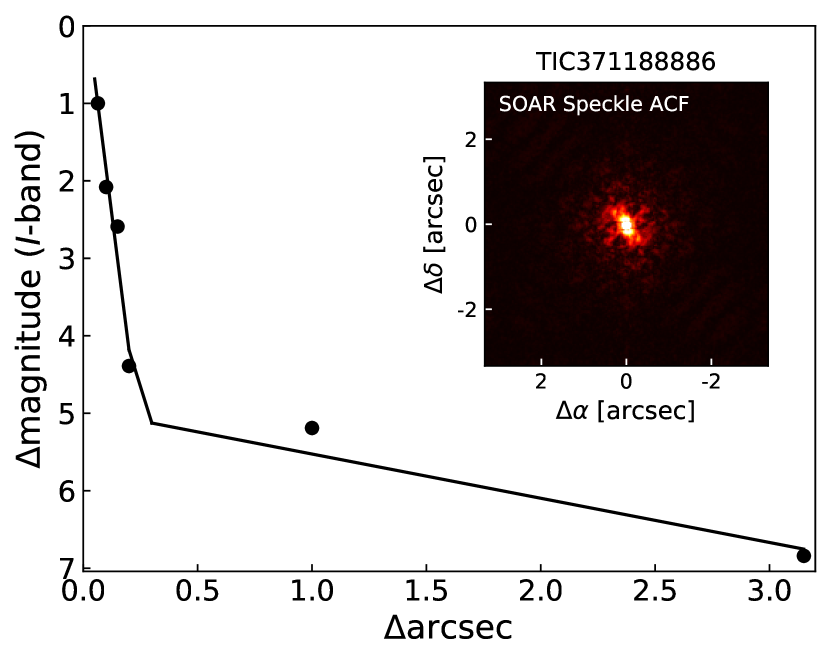
Figure 3: SOAR speckle observations of TOI-2000. The curve is the $5\sigma$ detection sensitivity, and the inset is the speckle imaging autocorrelation function (ACF). No companion is detected within the contrast limit.

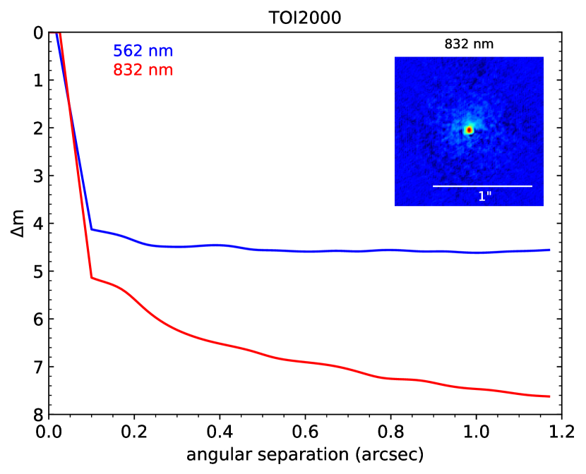
Figure 4: Gemini speckle observations of TOI-2000. The curves are the $5\sigma$ detection sensitivity in the $562\text{\,}\mathrm{nm}$ (blue) and $832\text{\,}\mathrm{nm}$ (red) bands, and the inset is the reconstructed speckle image in $832\text{\,}\mathrm{nm}$. No companion is detected within the contrast limit.

We searched for unresolved companions of TOI-2000 with speckle imaging from two telescopes on Cerro Pachón, Chile. The first set of data was acquired by the HRCam instrument (Tokovinin, 2018) on the 4.1-m Southern Astrophysical Research (SOAR) telescope on ut 2020 October 31. The observations were in a passband similar to TESS’s and were reduced with procedures described by Ziegler et al. (2020). No companion was found with a contrast of 6.8 magnitudes at $1^{\prime\prime}$. The $5\sigma$ sensitivity and the speckle autocorrelation function (ACF) from the observations are plotted in Figure 3.

The second set of speckle imaging data was acquired by the Zorro speckle instrument on the 8-m Gemini South telescope (Scott et al., 2021) on ut 2022 March 17. Zorro collected 20 sets of 1000 speckle imaging observations simultaneously in two bands ($562\text{\,}\mathrm{nm}$ and $832\text{\,}\mathrm{nm}$) with an integration time of $60\text{\,}\mathrm{ms}$ per frame. These thousands of observations were reduced using the method described by Howell et al. (2011), yielding a high-resolution view of the sky near TOI-2000. Figure 4 shows the two $5\sigma$ contrast curves and the reconstructed speckle image in $562\text{\,}\mathrm{nm}$ and $832\text{\,}\mathrm{nm}$. Again, we found no companion to TOI-2000 in the 832-nm band within a contrast of 5–8 magnitudes from $0.\mathrm{″}1$ to $1.\mathrm{″}2$ separation, which corresponds to a projected separation of $17.4208\text{\,}\mathrm{au}$ at the distance of TOI-2000 ($173.6\text{\,}\mathrm{pc}$).

3 Analysis

3.1 Stellar parameters

3.1.1 Spectral energy distribution

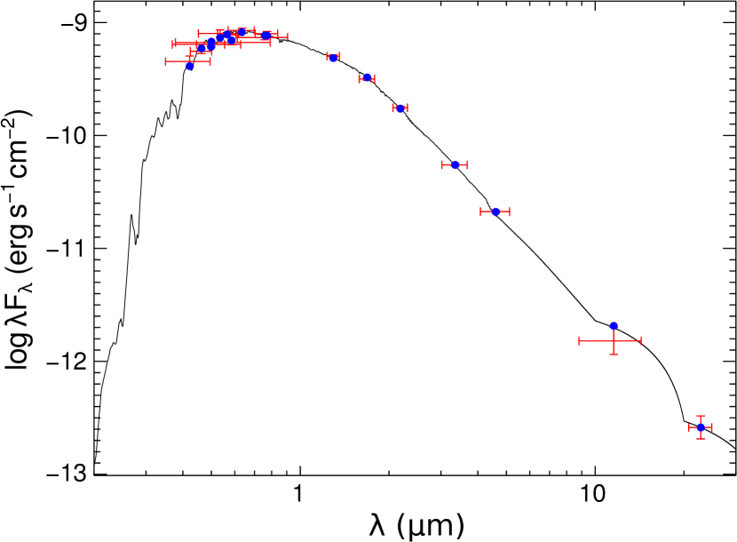
Figure 5: Spectral energy distribution of TOI-2000. Red symbols represent the observed photometric measurements, where the horizontal bars represent the effective width of the passband. Blue symbols are the model fluxes from the best-fitting Kurucz atmosphere model (black).

Independently of the obtained spectra in Section 2.2, we analysed the broadband spectral energy distribution (SED) of the star following the procedures described by Stassun & Torres (2016) and Stassun et al. (2017); Stassun et al. (2018a). We used the the $B$, $V$, $g^{\prime}$, $r^{\prime}$, $i^{\prime}$ magnitudes from APASS, the $J$, $H$, $K_{\mathrm{s}}$ magnitudes from 2MASS, the $W1$–$W4$ magnitudes from WISE, and the $G$, $G_{\mathrm{BP}}$, $G_{\mathrm{RP}}$ magnitudes from Gaia. Together, the available photometry spans the wavelength range $0.410\text{\,}\mathrm{\SIUnitSymbolMicro m}$ (Figure 5).

We fit the SED using Kurucz (1993) stellar atmosphere models, with effective temperature $T_{\text{eff}}$, metallicity $[\text{Fe}/\text{H}]$, and extinction $A_{V}$ as free parameters. We limited $A_{V}$ to the maximum line-of-sight value from the Galactic dust maps of Schlegel et al. (1998). The resulting best-fitting (reduced $\chi^{2}=1.2$) values are $T_{\text{eff}}{}=$5550\pm 75\text{\,}\mathrm{K}$$, $[\text{Fe}/\text{H}]{}=0.3\pm 0.2$, and $A_{V}=0.15\pm 0.04$. Integrating the unreddened SED model gives the bolometric flux at Earth $F_{\rm bol}=$(1.169\pm 0.014)\text{\times}{10}^{-9}\text{\,}\mathrm{erg}\text{\,}{\mathrm{s}}^{-1}\text{\,}{\mathrm{cm}}^{-2}$$. Together with the Gaia EDR3 parallax, the $F_{\rm bol}$ and $T_{\text{eff}}$ values imply a stellar radius $R_{\star}=$1.135\pm 0.031\text{\,}\mathrm{\mathrm{R}}_{\mathrm{\odot}}$$, consistent with the value from joint modelling (Section 3.3).

3.1.2 Spectroscopy and chemical abundances

Table 9: Chemical abundances of TOI-2000 with respect to the Sun.

Element (X)	[X/H]	Uncertainty
C i	0.26	0.02
O i	0.30	0.15
Mg i	0.44	0.06
Al i	0.52	0.04
Si i	0.43	0.03
Ca i	0.42	0.07
Ti i	0.47	0.06
Cr i	0.45	0.05
Ni i	0.50	0.05
Cu i	0.66	0.05
Zn i	0.45	0.03
Sr i	0.46	0.08
Y ii	0.34	0.07
Zr ii	0.28	0.04
Ba ii	0.25	0.03
Ce ii	0.37	0.06
Nd ii	0.40	0.03

We used ares+moog (Sousa, 2014; Santos et al., 2013) to obtain more precise stellar atmospheric parameters ($T_{\text{eff}}$, surface gravity $\log g$, microturbulence, $[\text{Fe}/\text{H}]$) from the combined HARPS spectrum of TOI-2000. The combined spectrum achieved an S/N of 275 at spectral order 60. We measured the equivalent widths of iron lines using the Automatic Routine for line Equivalent widths in stellar Spectra (ares) v2 code (Sousa et al., 2015). Then, we used a minimization process where we assumed ionization and excitation equilibrium to converge to the best set of spectroscopic parameters. This process made use of a grid of Kurucz (1993) model atmospheres and the radiative transfer code moog (Sneden, 1973), yielding the values $T_{\text{eff}}{}=$5568\pm 66\text{\,}\mathrm{K}$$, $[\text{Fe}/\text{H}]{}=0.438\pm 0.044$. These $T_{\text{eff}}$ and $[\text{Fe}/\text{H}]$ values were then used to constrain the MIST evolutionary track portion of the joint model (Section 3.3.2). We also used the Gaia EDR3 parallax measurement to derive a stellar surface gravity $\log g{}=4.38\pm 0.03$, consistent with the value independently derived by the joint model (Section 3.3). The spectroscopic $\log g$ was not used to constrain the joint model.

The combined HARPS spectrum also gave the abundances of various chemical elements in TOI-2000 (see Table 9). These abundances were derived from the same code and models as the stellar parameters, using classical curve of growth analysis assuming local thermodynamic equilibrium. For the derivation of abundances of refractory elements, we closely followed the methods described by Adibekyan et al. (2012); Adibekyan et al. (2015) and Delgado Mena et al. (2017). Abundances of the volatile elements C and O were derived following the methods of Delgado Mena et al. (2021) and Bertran de Lis et al. (2015). All the [X/H] ratios were calculated by differential analysis with respect to a high S/N Solar (Vesta) spectrum from HARPS.

These detailed abundances allowed us to measure the age of TOI-2000 through chemical clocks, or abundance ratios strongly correlated with age. We found the [X/Fe] ratios of TOI-2000 to be typical for a thin-disc star. Considering the variation in age due to $T_{\text{eff}}$ and $[\text{Fe}/\text{H}]$, we applied the 3D formulas described by Delgado Mena et al. (2019) in their Table 10 to calculate ages associated with the chemical clocks [Y/Mg], [Y/Zn], [Y/Ti], [Y/Si], [Y/Al], [Sr/Ti], [Sr/Mg], and [Sr/Si]. Their weighted average gave an independently measured age of $4.1\pm 1.6\text{\,}\mathrm{Gyr}$, within the uncertainty of the value from joint modelling (Section 3.3).

In addition to chemical abundances, we also measured the projected rotational velocity $v\sin i$ to be $2.99\pm 0.20\text{\,}\mathrm{km}\text{\,}{\mathrm{s}}^{-1}$ by performing spectral synthesis with moog on 36 isolated iron lines and by fixing the stellar parameters and limb-darkening coefficient (Costa Silva et al., 2020). The limb-darkening coefficient ($\approx 0.6$) was determined using the stellar parameters as described by Espinoza & Jordán (2015) assuming a linear limb darkening law.

3.2 Radial velocity variations

Since transits are sensitive only to planets with inclinations precisely aligned to our line of sight, it is possible additional planets may orbit in the TOI-2000 system but not be detected in the TESS observations. Therefore, we proceed to investigate whether additional planetary signals are present by computing and examining periodograms of our RV measurements.

3.2.1 Frequency analysis of RVs

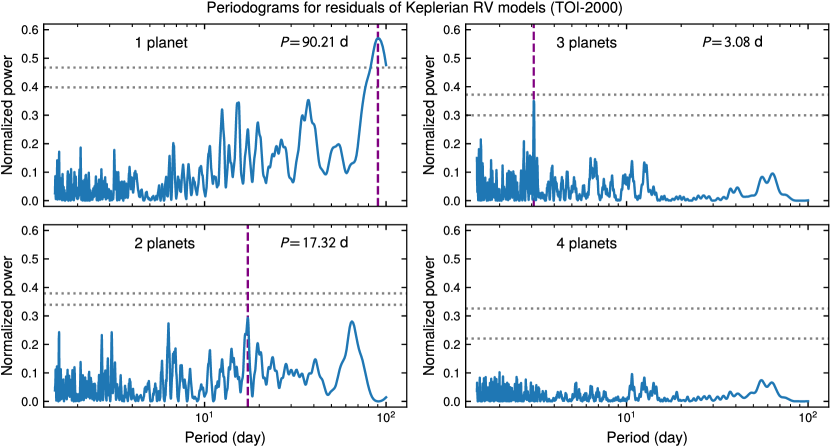
Figure 6: Periodograms of RV residuals after subtracting Keplerian signals. At each step, a Keplerian signal corresponding to the period peak in the previous periodogram is added. The vertical dashed purple line marks the most significant peak in the period interval from $1.5100\text{\,}\mathrm{d}$, and the horizontal dotted grey lines indicate the 1 and 0.1 per cent false-alarm levels computed with bootstrap resampling.

We investigate the possibility that there are signals for additional planets in the system in the RV measurements (Section 2.2). Starting from the first 9.1-d signal of TOI-2000 c, we iteratively remove new Keplerian signals at periodogram peaks. At each step, we calculate the Lomb–Scargle (LS; Lomb, 1976; Scargle, 1982) periodogram, fit for a new circular Keplerian (i.e. sinusoidal) signal at the next significant peak, remove the signal due to the new planet, and then recalculate the LS periodogram. Figure 6 shows this process. We found two additional periodogram peaks: a second one at $90.2\text{\,}\mathrm{d}$, which is highly formally significant based on the false-alarm probability (FAP) calculated by bootstrap resampling (see e.g. Ivezić et al., 2020), and a third one at $17.3\text{\,}\mathrm{d}$ (FAP $\approx 5$ per cent). After removing these two signals, we finally identify a fourth peak at $3.1\text{\,}\mathrm{d}$, which corresponds to the period of TOI-2000 b, with an FAP $\approx 1$ per cent.

Given these detections, we assess whether the two additional RV signals are viable planet candidates. Although both signals were detected before that of the transiting mini-neptune TOI-2000 b, there are reasons to caution that they may not be planetary. In particular, the 17.3-d signal has a relatively high FAP ($>1$ per cent). Although the 90-d signal is formally statistically significant, our observations cover fewer than two full phase cycles and consequently have yet to establish that the signal is repeating. Out of these considerations, we proceed to investigate alternative explanations for the additional two peaks at $17.390\text{\,}\mathrm{d}$, namely stellar activity and rotation, in the following subsections.

3.2.2 Correlation with stellar activity

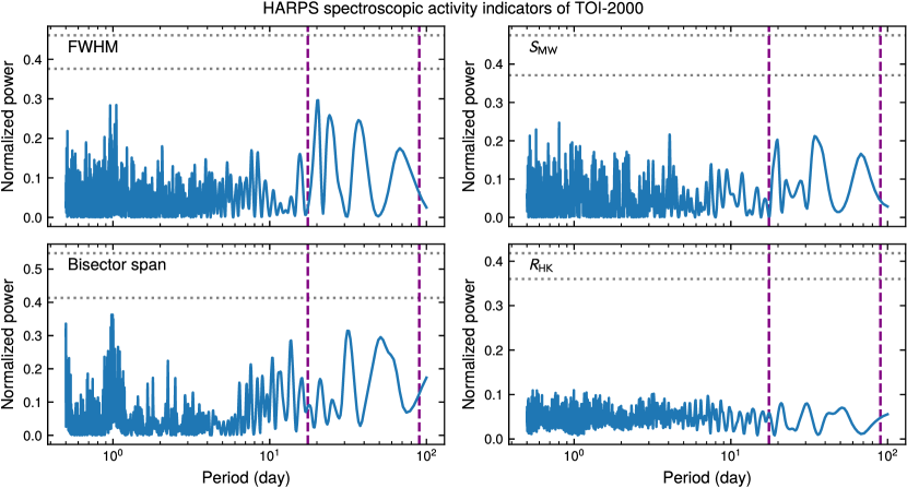
Figure 7: Lomb–Scargle periodograms of HARPS spectroscopic activity signals for TOI-2000. The activity signals are full-width half maximum (FWHM, Top Left), bisector span (Bottom Left), Mount Wilson $S$-index (Top Right), and spectral index of the Ca ii H and K lines $R_{\text{HK}}$ (Bottom Right). The two vertical dashed purple lines mark the periods of the RV signals at $17.390\text{\,}\mathrm{d}$, and the three horizontal dotted grey lines indicate the 1 and 0.1 per cent false-alarm levels computed from bootstrap resampling. There are no significant peaks at the periods of the candidate planets. The activity signals are tabulated in Table 14.

We check the standard stellar activity indicators from the HARPS RV measurements to test for the possibility that the two additional RV signals are due to stellar activity. Figure 7 shows LS periodograms of the HARPS full-width half maximum, bisector span, Mount Wilson $S$-index, and the $R_{\text{HK}}$ spectral index of Ca ii H and K lines. None of the four indicators show significant peaks corresponding to the RV signals at $17.390\text{\,}\mathrm{d}$.

3.2.3 Correlation with stellar rotation

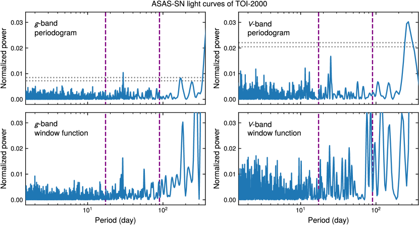
Figure 8: Lomb–Scargle periodogram of the ASAS-SN light curve of TOI-2000 in the $g$ (Left) and $V$ (Right) bands, with associated window functions (Bottom). The $x$-axis ranges from $1.5\text{\,}\mathrm{d}$ to $1\text{\,}\mathrm{yr}$. The two vertical dashed purple lines mark the period of the candidate non-transiting planets at $17.390\text{\,}\mathrm{d}$, and the two horizontal dotted grey lines indicate the 1 and 0.1 per cent false-alarm levels computed from bootstrap resampling. There is no significant peak that does not correspond to a peak in the window function, and there is no peak that corresponds to the 17.3 or 90-d RV signal.

As the TESS light curve of TOI-2000 does not show significant periodic variations, we check Wide Angle Search for Planets (WASP) and the All-Sky Automated Survey for Supernovae (ASAS-SN; Shappee et al., 2014) archival data for hints of the stellar rotation signal. There is no WASP light curve for TOI-2000, but ASAS-SN has light curves in the $g$ and $V$ bands spanning ut 2016 January 29 to 2023 February 14 (Kochanek et al., 2017). Figure 8 shows LS periodograms of the ASAS-SN light curves and their window functions. Again, no stellar rotation is detected, as there is no significant peak that does not correspond to a peak in the window function. In addition, the periodograms do not show peaks at the periods of the 17.3 and 90-d RV signals. Thus, we cannot determine whether the additional RV signals are associated with stellar rotation.

3.2.4 Two-planet vs. four-planet solutions

In the remainder of Section 3, we present models assuming two or more planets in the TOI-2000 system. In Section 3.3, we describe a two-planet solution that jointly models transits, RVs, and stellar parameters. In Section 3.4, we describe an alternative four-planet solution based on an RV-only model, compare it to the two-planet solution, and justify our present preference for the two-planet solution.

3.3 Joint modelling

Table 10: TOI-2000 stellar parameters.

Parameter Unit	Value		Prior	Source
Identifying Information
$\alpha$, right ascension (J2016) h:m:s	$09\mathrm{°}⁤45\mathrm{\prime }⁤35.\mathrm{″}289$		–	Gaia EDR3
$\delta$, declination (J2016) d:m:s	$-66\mathrm{°}⁤41\mathrm{\prime }⁤11.\mathrm{″}86$		–	Gaia EDR3
$\mu_{\alpha}$, R.A. proper motion $\mathrm{mas}\text{\,}{\mathrm{yr}}^{-1}$	$-73.219$	$\pm 0.012$	–	Gaia EDR3
$\mu_{\delta}$, decl. proper motion $\mathrm{mas}\text{\,}{\mathrm{yr}}^{-1}$	$12.623$	$\pm 0.012$	–	Gaia EDR3
TIC ID	371188886		–	TIC v8.2
Gaia EDR3 ID	5244434756689177088		–	Gaia EDR3
Photometric Properties
TESS mag	$10.358$	$\pm 0.006$	–	TIC v8.2
$V$ mag	$10.984$	$\pm 0.012$	–	TIC v8.2
$G$ mag	$10.85420$	$\pm 0.00016$	–	Gaia EDR3
Spectroscopic Properties
$v\sin i$, rotational speeda $\mathrm{km}\text{\,}{\mathrm{s}}^{-1}$	$2.99$	$\pm 0.20$	–	HARPS
Sampled Properties
$M_{\star,0}$, initial mass $\mathrm{\mathrm{M}}_{\mathrm{\odot}}$	$1.083$	${}_{-0.050}^{+0.059}$	$\sim\mathcal{U}(0.1,4)\,\mathcal{N}(1.05,0.2)$	–
$[\text{Fe}/\text{H}]_{0}$, initial metallicity dex	$0.417$	${}_{-0.041}^{+0.039}$	$\mathcal{U}(0,0.5)$	–
EEP, MESA equivalent evolutionary point …	$385$	${}_{-38}^{+24}$	$\mathcal{U}(202,454)$b	–
Parallax mas	$5.773$	$\pm 0.010$	$\mathcal{N}(5.773,0.010)$c	Gaia EDR3
$A_{V}$, extinction mag	$0.22$	$\pm 0.11$	$\mathcal{U}(0,0.70)$	Schlegel 1998
Derived Properties
$T_{\text{eff}}$, effective temperature K	$5611$	${}_{-82}^{+85}$	$\mathcal{N}(5568,100)\,\mathcal{N}(\text{MIST},3\%)$d	HARPS
$[\text{Fe}/\text{H}]$, metallicity dex	$0.439$	${}_{-0.043}^{+0.041}$	$\mathcal{N}(0.438,0.044)\,\mathcal{N}(\text{MIST},3\%)$d	HARPS
$\log g$, surface gravity dex($\mathrm{cm}\text{\,}{\mathrm{s}}^{-2}$)	$4.363$	${}_{-0.032}^{+0.034}$	–	–
$M_{\star}$, mass $\mathrm{\mathrm{M}}_{\mathrm{\odot}}$	$1.082$	${}_{-0.050}^{+0.059}$	–	–
$R_{\star}$, radius $\mathrm{\mathrm{R}}_{\mathrm{\odot}}$	$1.134$	${}_{-0.036}^{+0.037}$	$\mathcal{N}(\text{MIST},3\%)$d	–
$\rho_{\star}$, density $\mathrm{g}\text{\,}{\mathrm{cm}}^{-3}$	$1.047$	${}_{-0.100}^{+0.114}$	–	–
$L_{\star}$, bolometric luminosity $\mathrm{\mathrm{L}}_{\mathrm{\odot}}$	$1.147$	${}_{-0.084}^{+0.094}$	–	–
Age Gyr	$5.3$	$\pm 2.7$	$\mathcal{U}(0,10)$e	–
distance pc	$173.22$	$\pm 0.31$	–	–

^aNot part of the joint model, measured directly from HARPS spectra.

^bConstrains the star to be main sequence, which we know from spectroscopic analysis. The effective prior is uniform in age rather than EEP because the model likelihood is multiplied by $\partial(\mathrm{EEP})/\partial(\mathrm{age})$.

^cCorrected for the Gaia EDR3 parallax zero-point as a function of magnitude, colour, and position using the prescription of Lindegren et al. (2021).

^dAt each step of the HMC chain, the sampled values of $(M_{\star,0},[\text{Fe}/\text{H}]_{0},\mathrm{EEP})$ are used as the input to the MIST grid, which output $M_{\star,\text{MIST}}$, $\log g{}_{\star,\text{MIST}}$, $T_{\text{eff}}{}_{,\text{MIST}}$, $[\text{Fe}/\text{H}]_{\text{MIST}}$, and stellar age. These interpolated values are used to compute $R_{\star,\text{MIST}}$. The shorthand $\mathcal{N}(\text{MIST},3\%)$ means that the normal distribution is centred on the interpolated value of the MIST grid with a fractional uncertainty of 3%.

^eApproximated by adding a logistic function $f(x)=-10^{100}/(1+e^{-3000(x-10)})$ to the log-probability of the model.

Note. $\mathcal{U}(a,b)$ is the uniform distribution over the interval $[a,b]$. $\mathcal{N}(\mu,\sigma)$ is the normal distribution with mean $\mu$ and standard deviation $\sigma$. The values and uncertainties quoted are 68% credible intervals centred on medians.

References. Gaia EDR3: Gaia Collaboration et al. (2021). TIC v8.2: Stassun et al. (2019); Paegert et al. (2021). Schlegel 1998: Schlegel et al. (1998).

Table 11: TOI-2000 planetary system parameters.

Planet	b			c
Parameter Unit:	Value		Prior	Value		Prior
Sampled
$T_{\text{c}}$, time of conjunction BJD	$2458855.2442$	${}_{-0.0021}^{+0.0022}$	$2458855+\mathcal{U}(0.224,0.264)$	$2459110.06588$	${}_{-0.00028}^{+0.00027}$	$2459110+\mathcal{U}(0.0609,0.0709)$
$P$, period day	$3.098330$	${}_{-0.000019}^{+0.000021}$	$3.09833+\mathcal{U}(-2,2)\times 10^{-4}$	$9.1270550$	${}_{-0.0000072}^{+0.0000073}$	$9.127055+\mathcal{U}(-10^{-4},10^{4})$
$\sqrt{e}\cos\omega$	0		fixed	$-0.215$	${}_{-0.046}^{+0.061}$	$e<1$a
$\sqrt{e}\sin\omega$	0		fixed	$-0.06$	${}_{-0.12}^{+0.14}$	$e<1$a
$b\equiv a\cos(i)/R_{\star}$, impact parameter	$0.770$	${}_{-0.071}^{+0.038}$	$\mathcal{U}(0,1+R_{\text{p}}/R_{\star})$	$0.631$	${}_{-0.047}^{+0.039}$	$\mathcal{U}(0,1+R_{\text{p}}/R_{\star})$
$R_{\text{p}}/R_{\star}$	$0.02182$	${}_{-0.00097}^{+0.00089}$	$\mathcal{U}(0,0.5)$	$0.06581$	$\pm 0.00068$	$\mathcal{U}(0,0.5)$
$M_{\text{p}}/M_{\star}$	$(3.06$	$\pm 0.66)\times 10^{-5}$	$\mathcal{U}(0,2.8605\times 10^{-4})$b	$(2.26$	${}_{-0.12}^{+0.11})\times 10^{-4}$	$\mathcal{U}(0,8.5814\times 10^{-4})$b
Derived
$T_{14}$, total transit duration hour	$1.959$	${}_{-0.098}^{+0.209}$	–	$3.654$	${}_{-0.028}^{+0.030}$	–
$e$, eccentricity	0		fixed	$0.063$	${}_{-0.022}^{+0.023}$	–
$\omega$, argument of periastron deg	–		–	$196$	${}_{-34}^{+29}$	–
$a$, semimajor axis au	$0.04271$	${}_{-0.00067}^{+0.00076}$	–	$0.0878$	${}_{-0.0014}^{+0.0016}$	–
$a/R_{\star}$	$8.10$	${}_{-0.27}^{+0.28}$	–	$16.64$	${}_{-0.55}^{+0.59}$	–
$i$, inclination deg	$84.59$	${}_{-0.43}^{+0.54}$	–	$87.86$	${}_{-0.18}^{+0.19}$	–
$K$, RV semiamplitude $\mathrm{m}\text{\,}{\mathrm{s}}^{-1}$	$4.59$	${}_{-0.99}^{+1.00}$	–	$23.7$	${}_{-0.99}^{+1.00}$	–
$R_{\text{p}}$, radius $\mathrm{\mathrm{R}}_{\mathrm{\oplus}}$	$2.70$	$\pm 0.15$	–	$8.14$	${}_{-0.30}^{+0.31}$	–
$R_{\text{p}}$, radius $\mathrm{\mathrm{R}}_{\mathrm{J}}$	$0.241$	$\pm 0.014$	–	$0.727$	${}_{-0.027}^{+0.028}$	–
$M_{\text{p}}$, mass $\mathrm{\mathrm{M}}_{\mathrm{\oplus}}$	$11.0$	$\pm 2.4$	–	$81.7$	${}_{-4.6}^{+4.7}$	–
$M_{\text{p}}$, mass $\mathrm{\mathrm{M}}_{\mathrm{J}}$	$0.0347$	${}_{-0.0075}^{+0.0077}$	–	$0.257$	${}_{-0.014}^{+0.015}$	–
$\rho_{\text{p}}$, density $\mathrm{g}\text{\,}{\mathrm{cm}}^{-3}$	$3.07$	${}_{-0.78}^{+0.94}$	–	$0.829$	${}_{-0.096}^{+0.111}$	–
Stellar irradiation $\mathrm{erg}\text{\,}{\mathrm{s}}^{-1}\text{\,}{\mathrm{cm}}^{-2}$	$(8.55$	${}_{-0.59}^{+0.66})\times 10^{8}$	–	$(2.03$	${}_{-0.14}^{+0.16})\times 10^{8}$	–
$T_{\text{eq}}$, equilibrium temperaturec K	$1488$	${}_{-160}^{+122}$	–	$1038$	${}_{-111}^{+84}$	–

Table 12: Additional sampled joint model parameters.

Parameter Unit	Value		Prior
Limb darkening
$u_{1}$, TESS	$0.130$	${}_{-0.095}^{+0.170}$	Kipping
$u_{2}$, TESS	$0.32$	${}_{-0.24}^{+0.16}$	Kipping
$u_{1}$, $R_{\mathrm{c}}$	$0.89$	${}_{-0.28}^{+0.21}$	Kipping
$u_{2}$, $R_{\mathrm{c}}$	$-0.29$	${}_{-0.20}^{+0.33}$	Kipping
$u_{1}$, $z_{\mathrm{s}}$	$0.41$	${}_{-0.28}^{+0.35}$	Kipping
$u_{2}$, $z_{\mathrm{s}}$	$0.01$	${}_{-0.27}^{+0.32}$	Kipping
Photometry
Offset, TESS year 1	$(-1.3$	$\pm 1.2)\times 10^{-5}$	$\mathcal{U}(-0.5,0.5)$
Offset, TESS year 3	$(1.5$	$\pm 1.2)\times 10^{-5}$	$\mathcal{U}(-0.5,0.5)$
Jitter, TESS year 1	$(9.2$	${}_{-4.2}^{+3.1})\times 10^{-5}$	$\mathcal{U}(0,1)$
Jitter, TESS year 3	$(2.06$	${}_{-1.15}^{+0.87})\times 10^{-4}$	$\mathcal{U}(0,1)$
Jitter, ASTEP $R_{\mathrm{c}}$	$(1.25$	${}_{-0.87}^{+1.23})\times 10^{-4}$	$\mathcal{U}(0,1)$
Jitter, LCOGT SSO $z_{\mathrm{s}}$	$0.00123$	$\pm 0.00014$	$\mathcal{U}(0,1)$
Radial velocity
$\gamma$, CHIRON $\mathrm{m}\text{\,}{\mathrm{s}}^{-1}$	$6647.7$	${}_{-12.8}^{+8.8}$	$\mathcal{U}(5659.0,7659.0)$
$\gamma$, FEROS $\mathrm{m}\text{\,}{\mathrm{s}}^{-1}$	$8116$	${}_{-14}^{+11}$	$\mathcal{U}(7114.6,9114.6)$
$\gamma$, HARPS $\mathrm{m}\text{\,}{\mathrm{s}}^{-1}$	$8118.1$	${}_{-12.2}^{+8.2}$	$\mathcal{U}(7113.5,9113.5)$
Jitter, CHIRON $\mathrm{m}\text{\,}{\mathrm{s}}^{-1}$	$3.4$	${}_{-2.3}^{+3.2}$	$\sim\mathcal{U}(0,\infty)\,\mathcal{N}(0,15)$
Jitter, FEROS $\mathrm{m}\text{\,}{\mathrm{s}}^{-1}$	$14.0$	${}_{-3.3}^{+4.5}$	$\sim\mathcal{U}(0,\infty)\,\mathcal{N}(0,30)$
Jitter, HARPS $\mathrm{m}\text{\,}{\mathrm{s}}^{-1}$	$3.14$	${}_{-0.78}^{+0.82}$	$\sim\mathcal{U}(0,\infty)\,\mathcal{N}(0,15)$
Gaussian process for RV
$\rho$, undamped period day	$111$	${}_{-37}^{+57}$	$\mathcal{U}(15,200)$
$\tau$, damping timescale day	$37$	${}_{-31}^{+95}$	$\mathcal{U}(0,200)$
$\sigma$, standard deviation $\mathrm{m}\text{\,}{\mathrm{s}}^{-1}$	$21.4$	${}_{-7.6}^{+14.6}$	$\mathcal{U}(0,100)$
SED
$T_{\text{eff,SED}}$, effective temperature …K	$5687$	${}_{-133}^{+142}$	$\mathcal{N}(T_{\text{eff}}{},2.5\%)$
$R_{\star,\text{SED}}$, stellar radius $\mathrm{\mathrm{R}}_{\mathrm{\odot}}$	$1.103$	$\pm 0.014$	$\mathcal{U}(0,2R_{\star})$
SED uncertainty scaling factor	$1.27$	${}_{-0.20}^{+0.39}$	$\mathcal{U}(1,4)$

Note. The Kipping (2013) prior is a triangle sampling of the space of physically plausible quadratic limb darkening parameters. The RV parameters are reproduced in Table 7 for convenience. $\mathcal{U}(a,b)$ is the uniform distribution over the interval $[a,b]$. $\mathcal{N}(\mu,\sigma)$ is the normal distribution with mean $\mu$ and standard deviation $\sigma$. For an explanation of $T_{\text{eff,SED}}$, $R_{\star,\text{SED}}$, and the ‘SED uncertainty scaling factor’, see Section 3.3.3. The values and uncertainties quoted are 68% credible intervals centred on medians.

We constructed a joint model of the photometric light curves, RV measurements, metallicity, surface gravity, and broadband photometric magnitudes of TOI-2000 with the Python packages exoplanet (Foreman-Mackey et al., 2021b, a) and celerite2 (Foreman-Mackey et al., 2017; Foreman-Mackey, 2018) as well as the MIST stellar evolutionary tracks (Dotter, 2016; Choi et al., 2016). The model’s parameters included the orbital elements of the two planets (the inner planet b’s orbit is fixed to be circular), stellar parameters, limb-darkening parameters, Gaussian process (GP) parameters for modelling the long-term trend in RVs, and other observational nuisance parameters. The posterior distribution of these parameters was then sampled via Hamiltonian Monte Carlo (HMC; Duane et al., 1987) implemented by the PyMC probabilistic programming framework (Salvatier et al., 2016). The posteriors and priors of the joint model’s stellar, planetary, and other parameters are reported in Table 10, Table 11, and Table 12.

3.3.1 Light curve and RV models

We modelled the photometric observations with the quadratic law LimbDarkLightCurve class built into the exoplanet package. To account for long exposure time’s smearing effect on the shape of transit light curves, we oversampled each TESS 30-min exposure by a factor of $15$ but did not oversample the 20-s exposures. Among the ground-based photometry, we included two sets of observations with the best S/N, the ASTEP data in the $R_{\mathrm{c}}$ band and the LCOGT-SSO data in the $z_{\mathrm{s}}$ band, in the joint model. These light curves were simultaneously detrended using their respective ‘sky’ time series in Tables 6 and 4. We used separate sets of limb darkening parameters for each of the TESS, $R_{\mathrm{c}}$, $z_{\mathrm{s}}$ filters, each subject to the uniform triangular sampling prior of Kipping (2013).

We also used exoplanet’s built-in RV model. For each instrument, we introduced a constant RV offset $\gamma$ and a jitter term representing systematic uncertainty that is added in quadrature to the reported instrumental uncertainties. We modelled long-term variations in the RV residuals with a GP simple harmonic oscillator (SHO) kernel implemented by the celerite2 (Foreman-Mackey et al., 2017; Foreman-Mackey, 2018) Python package. The SHO kernel has a power spectral density of

$$S(\omega)=\sqrt{\frac{2}{\pi}}\frac{S_{0}\omega_{0}^{4}}{(\omega^{2}-\omega_{0}^{2})^{2}+\omega_{0}^{2}\omega^{2}/Q^{2}},$$ (1)

and we use a parameterization in terms of the undamped period of the oscillator $\rho=2\pi/\omega_{0}$, the damping timescale of the process $\tau=2Q/\omega_{0}$, and the standard deviation of the process $\sigma=\sqrt{S_{0}\omega_{0}Q}$. We require $\rho\geq$15\text{\,}\mathrm{d}$$ so that the GP does not interfere with the RV signals of the two planets at shorter periods. This exclusion of shorter periods is justified since we do not expect TOI-2000 to be rapidly rotating as it is a middle-aged Sun-like star, and there are no significant short-term periodic variations in the undetrended TESS light curves. In an RV-only model that uses Gaussian priors corresponding to the joint model posterior values in Table 11 for the planets’ period and time of conjunction, introducing GP with the SHO kernel causes the RV jitter of HARPS to decrease from $11.6$ to $3.1\text{\,}\mathrm{m}\text{\,}{\mathrm{s}}^{-1}$. Thus, the GP captures some of the long-term RV variations.

To ensure that the joint model’s ability to detect the RV signal of planet b is not sensitive to the choice of GP kernel, we also ran another model using the Matérn-3/2 kernel

$$k(\tau)=\sigma^{2}\left(1+\frac{\sqrt{3}\tau}{\rho}\right)\exp\!\left(-\frac{\sqrt{3}\tau}{\rho}\right),$$ (2)

where $\tau$ is the pairwise distance and $\sigma,\rho$ are arbitrary parameters. The Matérn-3/2 kernel did not lead to a meaningful difference in the sampled posterior distribution compared to the SHO kernel.

Even though the variations in the RV residuals are sufficiently captured by the GP model, which is customarily used to model correlated noise due to stellar activity, we cannot definitively establish that stellar activity is the cause of these variations. An alternative explanation is that the variations are due to undetected additional planets in the system, a possibility that we explore in Section 3.4.

3.3.2 MIST evolutionary track interpolation

We used exoplanet’s RegularGridInterpolator to interpolate the MIST stellar evolutionary tracks (Dotter, 2016; Choi et al., 2016) built into the isochrones Python package (Morton, 2015). We used the initial stellar mass $M_{\star,0}$, initial metallicity $[\text{Fe}/\text{H}]_{0}$, and equivalent evolutionary point (EEP) as inputs to the interpolated grid, which then output present values of $M_{\star}$, $[\text{Fe}/\text{H}]{}_{\text{MIST}}$, $T_{\text{eff}}{}_{,\text{MIST}}$, and $R_{\star,\text{MIST}}$. Although we sampled EEP instead of age, we multiplied the overall model likelihood by $\partial(\mathrm{EEP})/\partial(\mathrm{age})$ as was done by Eastman et al. (2019) for exofastv2 to guarantee that the prior distribution is uniform in stellar age rather than EEP. We restricted EEP to the main sequence because spectroscopic evidence indicated that the star was not evolved. We also constrained the stellar age to be $<$10\text{\,}\mathrm{G}\mathrm{y}\mathrm{r}$$, because Gaia EDR3 kinematics suggest that TOI-2000 is most likely in the Galactic thin disk. To ensure that the probability density of the model is continuous across the stellar age cutoff, an important consideration because HMC relies on partial derivatives of the model, we implemented the maximum-age constraint by adding a logistic function

$$f(x)=-\frac{10^{100}}{1+e^{-3000(x-10)}},$$ (3)

where $x$ is the stellar age in Gyr, to the log-probability of the model. The coefficients of the logistic function are chosen to be as large as possible in order to achieve a sharp cutoff, but not so large that its derivative exceeds what can be represented by IEEE double precision floating point numbers, which would cause HMC to fail.

To better reflect realistic uncertainties in theoretical modelling, we made the stellar radius $R_{\star}$, stellar effective temperature $T_{\text{eff}}$, and stellar metallicity $[\text{Fe}/\text{H}]$ independently sampled model parameters subject to Gaussian priors with a fractional width of 3 per cent centred on their respective interpolated MIST grid values, following how Eastman et al. (2019) sampled these parameters for exofastv2. However, $M_{\star}$ was taken directly from the interpolated grid value. This model can be represented in pseudocode as

$$(M_{\star,0},[\text{Fe}/\text{H}]{}_{0},\mathrm{EEP}) \mapsto(M_{\star},R_{\star,\text{MIST}},[\text{Fe}/\text{H}]{}_{\text{MIST}},T_{\text{eff}}{}_{,\text{MIST}}),$$ (4a)

$$R_{\star} \sim\mathcal{N}(R_{\star,\text{MIST}},0.03\,R_{\star,\text{MIST}}),$$ (4b)

$$[\text{Fe}/\text{H}]{} \sim\mathcal{N}([\text{Fe}/\text{H}]{}_{\text{MIST}},0.03\,[\text{Fe}/\text{H}]{}_{\text{MIST}}),$$ (4c)

$$T_{\text{eff}}{} \sim\mathcal{N}(T_{\text{eff}}{}_{,\text{MIST}},0.03\,T_{\text{eff}}{}_{,\text{MIST}}),$$ (4d)

where the variables on the left are sampled, the variables on the right are deterministically computed, the arrow $\mapsto$ represents interpolation of the MIST grid, and the relation $\sim$ represents draws from a prior distribution, which in this case is the normal distribution $\mathcal{N}(\mu,\sigma)$ with mean $\mu$ and standard deviation $\sigma$. In addition, we computed the likelihood of $[\text{Fe}/\text{H}]$ and $T_{\text{eff}}$ using the HARPS spectroscopic values in Section 3.1, but the uncertainty of the HARPS $T_{\text{eff}}$ was artificially inflated to $100\text{\,}\mathrm{K}$ to better represent the uncertainty of the atmospheric models used to derive it.

3.3.3 SED model

We interpolated the MIST bolometric correction, or BC, grid (Choi et al., 2016) to convert the bolometric magnitude computed from the joint model’s stellar parameters into broadband photometric magnitudes. For direct comparison with observed apparent magnitudes, we sampled parallax from a Gaussian prior based on the Gaia EDR3 value and uncertainty corrected for a zero-point offset dependent on magnitude, colour, and ecliptic latitude using the prescription of Lindegren et al. (2021). Independently from the SED analysis in Section 3.1.1, we computed the likelihood of the interpolated broadband magnitudes in the Gaia EDR3 $G$, $G_{\mathrm{RP}}$, and $G_{\mathrm{BP}}$ bands, the 2MASS $J$, $H$, and $K_{\mathrm{s}}$ bands, as well as the WISE $W1$–$W4$ bands using their observed values and uncertainties but applied an uncertainty floor of $0.02$ to the Gaia magnitudes. We also multiplied all photometric uncertainties by a multiplicative factor constrained to be between $1$ and $4$ in order to avoid overweighting the SED constraints within the joint model. This factor is named ‘SED uncertainty scaling factor’ in Table 12.

We wanted to ensure that the SED model does not constrain stellar parameters more precisely than the systematic uncertainty floors estimated by Tayar et al. (2022). We loosely followed the latest SED model construction of exofastv2 described by Eastman et al. (2022). The key was to partially decouple the stellar parameters used by the SED model, in particular the calculation of BC, from those used for the light curve and RV models or the MIST evolutionary tracks. To that end, we introduced additional sampled parameters $T_{\text{eff,SED}}$ and $R_{\star,\text{SED}}$, which are reported in Table 12. The SED radius $R_{\star,\text{SED}}$ was then combined with the $M_{\star}$ from interpolating the MIST track to calculate $\log g_{\text{SED}}$. The MIST-interpolated $[\text{Fe}/\text{H}]$ was used as is, and the extinction $A_{V}$ was sampled from a uniform prior with a lower limit of 0 and an upper limit given by Schlegel et al. (1998), which we notate as $\mathcal{U}(0,0.70)$. Altogether, four of these parameters formed the inputs to the interpolated BC grid as

$$A_{V} \sim\mathcal{U}(0,0.70),$$ (5a)

$$(M_{\star},R_{\star,\text{SED}}) \mapsto\log g_{\text{SED}},$$ (5b)

$$(T_{\text{eff,SED}},\log g_{\text{SED}},[\text{Fe}/\text{H}],A_{V}) \mapsto\mathrm{BC},$$ (5c)

using the notation of the pseudocode in Section 3.3.2.

To take account of the systematic uncertainty floors estimated for Solar-type stars by Tayar et al. (2022), the parameters $T_{\text{eff,SED}}$ and $R_{\star,\text{SED}}$ were partially coupled to the $T_{\text{eff}}$ and $R_{\star}$ adopted by the light curve and RV models. The parameter $T_{\text{eff,SED}}$ was coupled to the adopted $T_{\text{eff}}$ by a Gaussian prior with a 2.5 per cent width. Implicitly constraining $R_{\star,\text{SED}}$ was a 2-per-cent-wide Gaussian likelihood coupling the bolometric flux $F_{\text{bol,SED}}$ computed from $T_{\text{eff,SED}}$ and $R_{\star,\text{SED}}$ to $F_{\text{bol}}$ from the adopted $T_{\text{eff}}$ and $R_{\star}$. Using the notation of the pseudocode in Section 3.3.2,

$$T_{\text{eff,SED}} \sim\mathcal{N}(T_{\text{eff}},0.025T_{\text{eff}}{}),$$ (6a)

$$R_{\star,\text{SED}} \sim\mathcal{N}(0,2R_{\star}),$$ (6b)

$$(T_{\text{eff,SED}},R_{\star,\text{SED}},\varpi) \mapsto F_{\text{bol,SED}},$$ (6c)

$$(T_{\text{eff}},R_{\star},\varpi) \mapsto F_{\text{bol}},$$ (6d)

$$F_{\text{bol,SED}} \propto\mathcal{N}(F_{\text{bol}},0.02F_{\text{bol}}),$$ (6e)

where $\varpi$ is the parallax and the relation $\propto$ indicates likelihood. Converting the $F_{\text{bol,SED}}$ to apparent bolometric magnitude and subtracting the BC gave the predicted broadband photometric magnitudes that were compared to observations.

3.3.4 Sampling the posterior distribution

We ran PyMC’s HMC No-U-Turn Sampler (NUTS; Hoffman & Gelman, 2014) for 4096 tuning steps and 4096 draws on 32 independent chains. The resulting samples converged well, with the convergence statistic of Gelman & Rubin (1992) $\hat{R}\approx 1$ and effective sample sizes ranging from $830095\,000$ across all parameters and chains as calculated by the arviz Python package (Kumar et al., 2019). The median and the middle 68 per cent credible interval of the posterior distribution, as well as the prior distribution of each fitted parameter, are reported in Tables 10, 11, and 12.

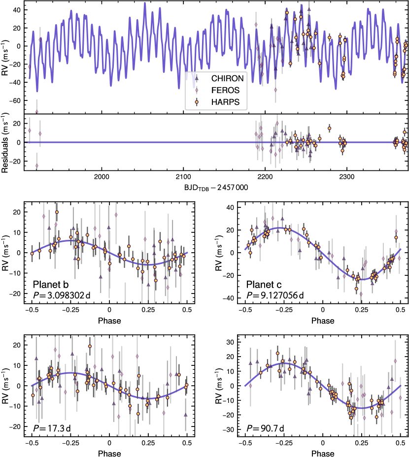
Figure 9: Alternative four-planet model of the RV measurements of TOI-2000. The shape and colour of each mark indicate which spectrograph it corresponds to, and its error bar is the quadrature sum of uncertainty and an instrumental jitter term. Solid purple lines represent the median-posterior RV model. Top: The median-posterior RV model and the residuals of the RV measurements with respect to the model. Middle: Phase-folded RV variations due to planets b and c only. Bottom: Phase-folded RV variations due to the hypothetical non-transiting planets only.

3.4 Alternative RV model with additional planets

To explore alternative interpretations for the RV residuals not explained by the two transiting planet candidates, we modelled their variations as additional non-transiting planets in the system. We ran two RV-only models: a three-planet model with the third planet around a 90-day orbital period, and a four-planet model with an additional fourth planet around a 17-day period. These periods corresponded to the next two most significant peaks in the Lomb–Scargle periodogram of the RVs after the signal due to the hot saturn at 9.13 d was removed. For these RV-only models, the periods and times of conjunction of the two inner planets were drawn from Gaussian prior distributions with means and standard deviations corresponding to those of the posterior of the joint model in Section 3.3. The eccentricity $e$ and argument of periapsis $\omega$ of the 9.13-day hot saturn were free parameters, with a uniform prior in the unit disc of $(\sqrt{e}\cos\omega,\sqrt{e}\sin\omega)$, but the other three planets’ orbits were fixed to be circular.

The resulting median-posterior four-planet RV model is presented in Figure 9. As measured by the four-planet model, the proposed two outer planets have periods $17.29^{+0.09}_{-0.12}\text{\,}\mathrm{d}$ and $90.7^{+1.6}_{-1.5}\text{\,}\mathrm{d}$ and RV semiamplitudes $5.3\pm 1.1\text{\,}\mathrm{m}\text{\,}{\mathrm{s}}^{-1}$ and $15.4\pm 1.2\text{\,}\mathrm{m}\text{\,}{\mathrm{s}}^{-1}$, corresponding to minimum masses ($M_{\text{p}}\sin i$) $26.9\pm 4.8\text{\,}\mathrm{\mathrm{M}}_{\mathrm{\oplus}}$ and $114.1^{+10.2}_{-9.8}\text{\,}\mathrm{\mathrm{M}}_{\mathrm{\oplus}}$. We do not show the three-planet model here because it has significantly higher instrumental jitters compared to the four-planet model. For CHIRON, FEROS, and HARPS, respectively, the three-planet model has jitters $4.2^{+3.6}_{-2.8}\text{\,}\mathrm{m}\text{\,}{\mathrm{s}}^{-1}$, $14.6^{+4.4}_{-3.3}\text{\,}\mathrm{m}\text{\,}{\mathrm{s}}^{-1}$, and $5.93^{+0.94}_{-0.79}\text{\,}\mathrm{m}\text{\,}{\mathrm{s}}^{-1}$, while the four-planet model has $4.0^{+3.4}_{-2.7}\text{\,}\mathrm{m}\text{\,}{\mathrm{s}}^{-1}$, $12.3^{+3.9}_{-3.0}\text{\,}\mathrm{m}\text{\,}{\mathrm{s}}^{-1}$, and $3.60^{+0.80}_{-0.69}\text{\,}\mathrm{m}\text{\,}{\mathrm{s}}^{-1}$.

Nevertheless, the evidence for the two additional signals in our RV data is not conclusive (Section 3.2). The longest contiguous RV time baseline covers just a little more than one period of the 90-day planet (from approximately $\mathrm{BJD}_{\text{TDB}}$ 2459189 to 2459298), so it is difficult to assess if the signal of the proposed 90-day planet is truly periodic. Moreover, due to the sparsity of data, we cannot rule out that non-transiting planets of a different combination of orbital periods are the true sources of the 90-day and 17-day signals. We conclude that our present RV data is insufficient for confidently claiming the detection of these two additional planets in the RVs.

Thus, in the absence of overwhelming evidence for the two additional RV-only planets, we chose to adopt planetary and stellar parameters from the the joint model with GP. Compared to the four-planet RV-only model, the two-planet GP-based joint model prefers a slightly lower mass for the 3.1-day mini-neptune by about 23 per cent ($1.3\sigma$). However, this difference would not change the qualitative characterization of the inner planet as a mini-neptune that we discuss in Section 5.1.

4 Confirmation of planetary candidates

4.1 Characteristics of TOI-2000 c

TOI-2000 c is a hot saturn with a radius of $8.14$${}_{-0.30}^{+0.31}$ $\mathrm{\mathrm{R}}_{\mathrm{\oplus}}$ and a mass of $81.7$${}_{-4.6}^{+4.7}$ $\mathrm{\mathrm{M}}_{\mathrm{\oplus}}$ in a $9.1270550$${}_{-0.0000072}^{+0.0000073}$-day orbit. We detected an eccentricity of $0.063$${}_{-0.022}^{+0.023}$, and the posterior distribution slightly favours a non-zero eccentricity at the 2–$3\sigma$ level. The mass and eccentricity were measured from a combination of 41 HARPS observations, 14 FEROS observations and 15 CHIRON observations. Each RV instrument independently detected a strong signal that was consistent with a companion of planetary mass at the period corresponding to the transit signal. In addition, ground-based observations showed that the transit signal of TOI-2000 c was on target and consistent with the depth measured by TESS. The Gemini/Zorro speckle imaging did not reveal any nearby stellar companions down to $\Delta\mathrm{mag}=5$ at an angular separation more than $0.\mathrm{″}1$ (projected separation of $17.4\text{\,}\mathrm{au}$) away from the star. Therefore, we confirm that TOI-2000 c is a planet with high confidence.

4.2 Characteristics of TOI-2000 b

TOI-2000 b is a mini-neptune with a radius of $2.70$$\pm 0.15$ $\mathrm{\mathrm{R}}_{\mathrm{\oplus}}$ and a mass of $11.0$$\pm 2.4$ $\mathrm{\mathrm{M}}_{\mathrm{\oplus}}$ in a $3.098330$${}_{-0.000019}^{+0.000021}$-day orbit, which corresponds to an RV semiamplitude of $4.59$${}_{-0.99}^{+1.00}$ $\mathrm{m}\text{\,}{\mathrm{s}}^{-1}$. In an RV-and-GP-only model that does not require the RV semiamplitude to be strictly positive, the $4\sigma$ lower limit is $0.39\text{\,}\mathrm{m}\text{\,}{\mathrm{s}}^{-1}$. This simplified model uses Gaussian priors corresponding to the joint model posterior values in Table 11 for the planets’ orbital period and time of conjunction and constrains the undamped period of the GP kernel to $>15\,\text{d}$, more than either planet’s period. This result is independent of the choice of either the SHO or the Matérn-3/2 kernel for GP.

Ordinarily, an independent RV detection suffices to confirm transiting planet candidates. In the case of TOI-2000 b, however, because of its relatively small transit depth ($\approx 470\,\text{ppm}$) and low measured RV semiamplitude ($4.59$${}_{-0.99}^{+1.00}$ $\mathrm{m}\text{\,}{\mathrm{s}}^{-1}$), we apply extra scrutiny to possible false positive scenarios.

4.3 False-positive analysis of TOI-2000 b

There are two main classes of false positive transiting planet candidates: instrumental artefacts and astrophysical signals that mimic transiting planets. We can rule out the possibility that TOI-2000 b is due to an instrumental artefact because the transit detection is robust across different observational campaigns and data reduction software. Transits occurred periodically and at a consistent depth during both the first and third years of TESS observations at 30-min or 20-s cadences. Both the qlp and the SPOC pipeline independently detected the transits of TOI-2000 b as a threshold-crossing event during their multi-year transit planet searches. Using an approach independent of the standard SPOC pipeline and qlp, we also decorrelated the TESS light curves from the spacecraft pointing quaternion time series (Section 2.1.1), thereby removing variations caused by spacecraft pointing jitter, a common source of instrumental systematics. Thus, it is highly unlikely that the transit signal was an instrumental artefact.

Having ruled out instrumental artefacts, there are four possible scenarios for astrophysical false positives. We will eliminate them one by one in the following subsubsections through statistical validation.

4.3.1 Is TOI-2000 an eclipsing binary (EB)?

We consider the scenario that the transit signal of TOI-2000 b is due to a grazing EB. Our RV analysis shows that TOI-2000 b is well below stellar mass if it indeed orbits its host star. In an RV-only model that does not fit for long-term trends with GP and uses Gaussian priors corresponding to the joint model posterior values in Table 11 for the planets’ period and time of conjunction, the $5\sigma$ upper limit of TOI-2000 b’s RV semiamplitude is $13.1\text{\,}\mathrm{m}\text{\,}{\mathrm{s}}^{-1}$, corresponding to a mass of $31.4\text{\,}\mathrm{\mathrm{M}}_{\mathrm{\oplus}}$, less than $0.1\text{\,}\mathrm{\mathrm{M}}_{\mathrm{J}}$. Thus, we can confidently rule out the EB scenario.

4.3.2 Is light from a physically associated companion blended with TOI-2000?

In this scenario, an EB or transiting planetary system that is gravitationally bound to TOI-2000 is the true source of the transit signal of TOI-2000 b. We use the molusc tool from Wood et al. (2021) to rule out potential bound companions with a Monte Carlo method. The molusc tool starts by randomly generating two million companions of stars or brown dwarfs according to physically motivated prior distributions of mass and orbital parameters. The expected observational effect of each companion is then compared with Gaia imaging, the scatter of Gaia astrometric measurements (parameterized by the renormalized unit weight error, or RUWE, metric), RVs, and the contrast curve from Gemini/Zorro speckle imaging. The surviving companions, which are not ruled out by the observational constraints, are the samples for the posterior distribution. Using the RVs and Gemini South contrast curve, molusc finds that about 23 per cent of generated companions survive regardless of whether the generated companion is restricted to impact parameter $<1$, and that objects with mass $>$0.1\text{\,}\mathrm{\mathrm{M}}_{\mathrm{\odot}}$$ are almost completely ruled out at periods $<$1000\text{\,}\mathrm{d}$$, equivalent to orbital separations $<$2\text{\,}\mathrm{au}$$. Thus, we can rule out most, but perhaps not all the possible physically associated EBs or transiting planetary systems.

To incorporate information from the shape of the transit light curve, we turn to triceratops by Giacalone et al. (2021). The triceratops tool uses the TESS light curve and the Gemini/Zorro contrast curve to calculate the marginal likelihoods of various scenarios that could potentially cause the transit-like signal that we attribute to TOI-2000 b. The marginal likelihood of each scenario is then scaled by appropriately chosen priors to produce the Bayesian posterior probability that the transit-like signal is produced by that scenario. Considering all the false positive scenarios featuring an unresolved bound companion, triceratops finds the probability to be $0.0073\pm 0.0002$.

4.3.3 Is light from a resolved and unassociated background system blended with TOI-2000?

In this scenario, a chance alignment of the foreground star TOI-2000 with a binary system in the Galactic background caused the signal to be wrongly identified with the foreground. A nearby EB that is no more than $8.3$ magnitudes fainter than TOI-2000 is needed to produce the $\approx 470\,\text{ppm}$ transit depth. A ground-based photometric observation on ut 2021 February 6 from LCOGT CTIO during the transit window of TOI-2000 b confidently rules out that the transit signal appears on nearly all nearby resolved stars of sufficient brightness, with the sole exception of TIC 845089585 ($\Delta\mathrm{mag}=8.71$ in TESS band, $5.\mathrm{″}32$ separation at a position angle of $3.\mathrm{°}96$). Nevertheless, triceratops rules out that TIC 845089585 was the source of the signal. The nearby false-positive probability arising from TIC 845089585 is $(3.02\pm 0.06)\times 10^{-12}$, virtually zero.

There is also the possibility that the transit signal of TOI-2000 b was contaminated by EBs falling on the same TESS CCD as TOI-2000 but outside of its immediate vicinity. Whilst this type of contamination was common during the Kepler mission (e.g. due to crosstalk or charge transfer inefficiency; see Coughlin et al., 2014), it is unlikely to apply to TESS observations of TOI-2000. Across multiple TESS sectors, the field of view rotated relative to the orientation of the CCDs, so any contaminating source would not be able to affect TOI-2000 consistently. Furthermore, the transit depth is consistent between photometry using a 1-pixel aperture versus larger apertures, providing strong evidence that the signal was indeed localized on the CCD. For these reasons, we only consider contaminating sources in the immediate vicinity of TOI-2000 for the false-positive analysis in this section.

4.3.4 Is light from an unresolved and unassociated background system blended with TOI-2000?

The analysis above rules out on-target EBs, bound companions, and nearby EBs but not unresolved background EBs arising from chance alignment. As the proper motion of TOI-2000 is too small for archival Digitized Sky Survey images to reveal the background under its current position, we turn to triceratops once more to quantify how likely the remaining scenarios are. To generate a population of simulated unresolved background stars in a $0.1\,\text{deg}^{2}$ region of the sky, triceratops uses the TRILEGAL galactic model (Girardi et al., 2005) and considers all simulated stars with TESS magnitudes fainter than that of the target star and brighter than $21$ (Giacalone et al., 2021). For false-positive scenarios involving these simulated background stars, triceratops finds a probability of $0.0020\pm 0.0001$.

4.3.5 TOI-2000 b is a confirmed planet

Altogether, triceratops gives a false-positive probability (FPP) of $0.0094\pm 0.0002$. Because the inner planet has been detected by the TESS SPOC pipeline, this FPP can be further divided by the multiplicity boost of $\approx 20$ calculated using the TOI catalogue from the TESS prime mission (Guerrero et al., 2021), which puts the final FPP ($\approx 0.0005$) at well below any reasonable threshold for validated planets (e.g. $<0.015$; Giacalone et al., 2021). This highly confident statistical validation, in addition to the $>4\sigma$ RV detection, is overwhelming evidence in favour of a small inner planet orbiting TOI-2000.

5 Discussion

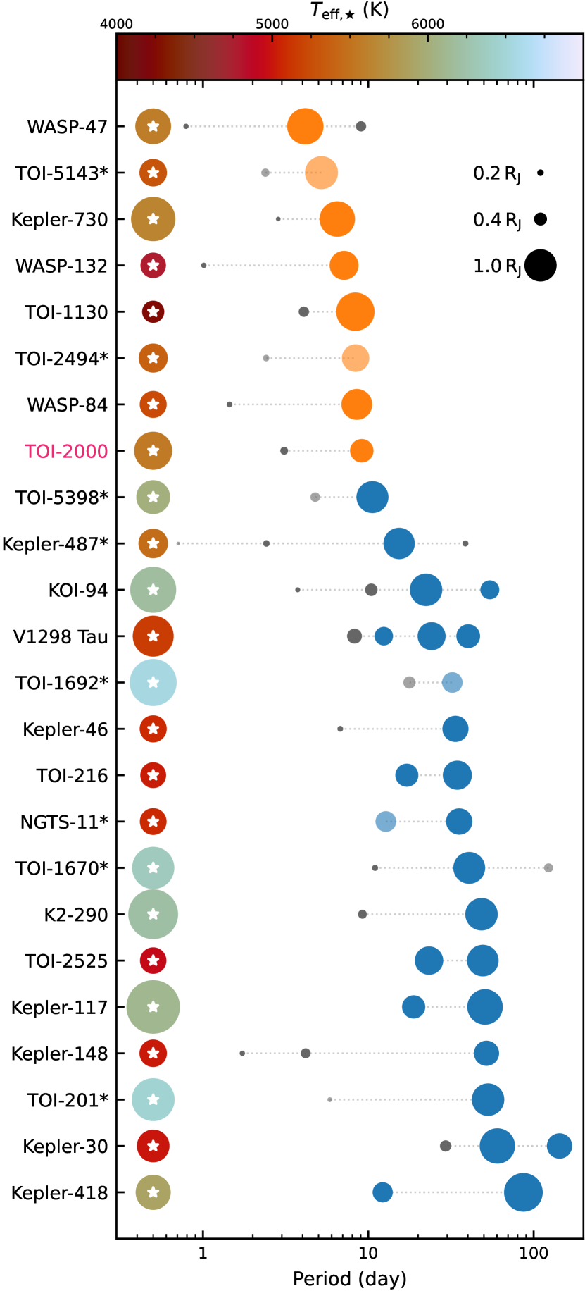
Figure 10: Transiting planetary systems hosting small planets orbiting interior to giant planets ($P<100\,\text{d}$). Non-transiting planets in these systems are omitted. The leftmost circle in each row represent the host star, with the mark’s linear size proportional to the stellar radius and fill colour indicating the effective temperature (from TIC 8.1; Stassun et al., 2019). The solid circles represent the transiting planets in the system, with their linear sizes proportional to planetary radii and fill colours indicating whether the planet is a giant planet (orange, $P<10\,\text{d}$; blue, $P\geq 10\,\text{d}$) or a small planet (grey, $R<$6\text{\,}\mathrm{\mathrm{R}}_{\mathrm{\oplus}}$$). The relative mark sizes among either the stars or the planets are to scale, but not between a star and its planets. The slightly translucent marks are planet candidates. Systems with an asterisk appended to their names contain planet candidates. The systems are sorted in ascending order of the period of the largest planet from top to bottom. Table 13 contains the numbers and references underlying this figure.

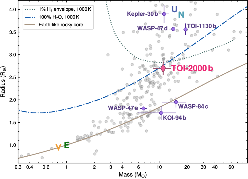
Figure 11: Mass–radius relationship of small exoplanets ($<$4\text{\,}\mathrm{\mathrm{R}}_{\mathrm{\oplus}}$$). Only planets with mass determination better than 33% have been included. The values used are the ‘default parameter set’ of the Planetary Systems Table from the NASA Exoplanet Archive (Akeson et al., 2013; NASA Exoplanet Archive, 2022, accessed on 2022 August 19). The mini-Neptune TOI-2000 b, together with six small planets WASP-47 d and e (Bryant & Bayliss, 2022), TOI-1130 b (Korth et al., 2023), WASP-84 c (Maciejewski et al., 2023), Kepler-30 b (Sanchis-Ojeda et al., 2012), and KOI-94 b (also known as Kepler-89; Weiss et al., 2013), which are also found in systems with giant planets, are highlighted, with error bars representing quoted uncertainties. The single letters denote the Solar System planets Venus, Earth, Uranus, and Neptune. Three theoretical mass–radius curves by Zeng et al. (2019, available online at https://lweb.cfa.harvard.edu/~lzeng/planetmodels.html) are plotted for reference: solid brown for an Earth-like rocky core (32.5% Fe and 67.5% $\text{MgSiO}_{3}$), dotted-dash blue for an 100% water world at $1000\text{\,}\mathrm{K}$, and dotted teal for a planet with 1% hydrogen envelope and 99% Earth-like rocky core at $1000\text{\,}\mathrm{K}$.

5.1 Diversity among inner companions to transiting gas giants

The TOI-2000 system hosts the smallest transiting hot gas giant planet ($P<$10\text{\,}\mathrm{d}$,M>$60\text{\,}\mathrm{\mathrm{M}}_{\mathrm{\oplus}}$$) known to have an inner companion. The hot gas giant TOI-2000 c has mass and radius similar to those of Saturn (Section 4.1) and has roughly the same mean density as WASP-132 b ($0.84\text{\,}\mathrm{g}\text{\,}{\mathrm{cm}}^{-3}$, Hellier et al., 2017), in contrast to the larger WASP-47 b, Kepler-730 b, and TOI-1130 c, which all have radii $\approx$1.1\text{\,}\mathrm{\mathrm{R}}_{\mathrm{J}}$$. The companion TOI-2000 b is a mini-neptune (Section 4.3) whose size sits between the three super-earth-sized companions (Kepler-730 c, WASP-47 e, and WASP-132 c) and the Neptune-sized TOI-1130 b.

The mean density of TOI-2000 b stands out among the handful of gas giant inner companions that have measured masses. Among the 23 confirmed or candidate transiting planetary systems that contain small planets ($<$4\text{\,}\mathrm{\mathrm{R}}_{\mathrm{\oplus}}$$) orbiting interior to gas giants of any period (Figure 10), only six small planets other than TOI-2000 b have measured mass (Figure 11). The densities of three of these planets, WASP-47 e, KOI-94 b, and WASP-84 c, are consistent with them being exposed rocky cores. The other three planets, Kepler-30 b, WASP-47 d, and TOI-1130 b, have masses and radii comparable to those of Neptune and Uranus. Whilst TOI-2000 b is not dense enough to be an exposed rocky core, its atmospheric mass fraction is likely considerably smaller than those of the three Neptune-sized planets, further demonstrating that these rare inner companions to giant planets are just as diverse in density as other small planets.

The qualitative results in this subsection would not change if we had adopted the alternative four-planet model (Section 3.4, Figure 9) instead of the two planets plus GP model (Figure 2) for the RVs. Respectively for TOI-2000 b and TOI-2000 c, the four-planet model gives RV semiamplitudes $5.9\pm 1.0\text{\,}\mathrm{m}\text{\,}{\mathrm{s}}^{-1}$ and $22.8\pm 1.0\text{\,}\mathrm{m}\text{\,}{\mathrm{s}}^{-1}$, corresponding to planet masses $14.3^{+2.6}_{-2.5}\text{\,}\mathrm{\mathrm{M}}_{\mathrm{\oplus}}$ and $78.3^{+4.7}_{-4.6}\text{\,}\mathrm{\mathrm{M}}_{\mathrm{\oplus}}$. Compared to these values, the posterior values from the joint model (Section 3.3) is smaller by $1.3\sigma$ for the mass of TOI-2000 b and larger by $0.7\sigma$ for the mass of TOI-2000 c. Regardless of whether this difference is statistically significant for TOI-2000 b, it is far short of what is needed to make TOI-2000 b a rocky core instead. The alternative location of TOI-2000 b on the mass–radius diagram is still intermediate between the rocky and the Neptune-sized planets.

5.2 Expected transit timing variations

We expect TTVs to be present in the TESS light curves of TOI-2000, as the periods of TOI-2000 c and TOI-2000 b are within 1.8 per cent of an exact 3:1 ratio and the orbit of TOI-2000 c is probably slightly eccentric (Section 4.1). Drawing from an ensemble of orbital parameters and planetary masses, we estimate the peak-to-peak TTV amplitude of TOI-2000 b to be 3–30 min with a superperiod $\approx 168$ d using TTVFast (Deck et al., 2014). The eccentricity vector and mass of TOI-2000 c and the mass of TOI-2000 b are drawn from the joint modelling posterior distribution (Section 3.3), and the eccentricity of TOI-2000 b is drawn from a Rayleigh distribution with a width of $0.06$. The TTV amplitude TOI-2000 c is similarly estimated to be $<5\,\text{min}$. This wide range of expected TTV amplitudes is attributable to uncertainties in the eccentricities and TTV phases of the two planets. However, the extremely shallow transit depth ($\approx 470\,\text{ppm}$) of TOI-2000 b makes it challenging to directly measure TTV from its individual transits in the TESS data.

In order to compare the simulated TTV effect to observation despite lacking a firm TTV detection, we instead measure the difference in the average time of conjunction $T_{\text{c}}$ for each year of TESS observations using the same set of TTVFast calculations, similar to the method employed by Mills et al. (2016). The resulting difference of 0.5–7 minutes is comparable to the joint model’s uncertainty of 3 minutes in the $T_{\text{c}}$ of TOI-2000 b. Whilst we are unable to prove or rule out the existence of TTVs in current TESS data, TESS will observe TOI-2000 again during its Extended Mission 2 in sectors 63–65 (ut 2023 March 10 – June 2), which will undoubtedly improve the S/N for TTV detection.

5.3 Opportunities for atmospheric characterization

The TOI-2000 system currently provides the second best opportunity for measuring the atmospheric compositions of a hot gas giant and small inner planet together, which potentially provide us with insight into where they formed within their protoplanetary disc. The JWST transmission spectrum metric (TSM; Kempton et al., 2018) for TOI-2000 b and c are 29 and 68, respectively. Although TOI-2000 is brighter in the $V$ band, its TSMs trail those of the TOI-1130 system because that system has a smaller host star brighter in the $J$ band and bigger planets. The host star TOI-1130 is a K dwarf rather than a G dwarf like TOI-2000, and its inner planet TOI-1130 b is approximately 40 per cent larger than TOI-2000 b. However, that TOI-1130 b shows TTV with peak-to-peak amplitude of at least two hours (Korth et al., 2023) means that an accurate ephemeris based on $N$-body numerical integration must be available, unlike TOI-2000 b, which does not conclusively show TTV at the present level of photometric precision (Section 5.2).

Measuring the atmospheric metallicity of both planets could help us understand their structure and origin. Using CEPAM (Guillot & Morel, 1995; Guillot et al., 2006) and a non-grey atmosphere (Parmentier et al., 2015), we model the evolution of both planets in the system assuming a simple structure consisting of a central rocky core surrounded by a H–He envelope of Solar composition. Under this model, the core mass of TOI-2000 c is between $36$ and $46\text{\,}\mathrm{\mathrm{M}}_{\mathrm{\oplus}}$, about twice as large as Saturn’s total mass of heavy elements ($16.5$ to $21\text{\,}\mathrm{\mathrm{M}}_{\mathrm{\oplus}}$; Mankovich & Fuller, 2021). The presumed H–He envelope of TOI-2000 b must be smaller than $0.1\text{\,}\mathrm{\mathrm{M}}_{\mathrm{\oplus}}$ (1 per cent of the mass of the planet), in line with Figure 11, which indicates that the radius of TOI-2000 b is up to 10 per cent smaller than the radius predicted by the theoretical mass–radius curve of Zeng et al. (2019) for planets with 1 per cent $\text{H}_{2}$ envelope. Overall, this analysis implies that both planets likely contain a proportion of heavy elements that is significantly larger than that of planets with similar mass in the Solar System.

By comparing the atmospheric abundances of two planets around the same host star, we can infer whether they formed at disc locations with similar compositions. The atmospheres of short-period planets forming in situ should contain more refractory metals (Fe, Cr, Ti, VO, Na, K, and P), which are more abundant closer to the host star, than volatile elements (O, C, and N). Even though it is unlikely that measured atmospheric abundances alone could pinpoint where a planet formed in its disc, such as with the method suggested by Öberg et al. (2011), we can still distinguish scenarios where the gas giant and the small planet formed together far from the host star (i.e. beyond the snow line) from others where the gas giant formed first and then swept material near its orbital resonances on its migration path to form the small planet. The former scenario would result in two planets of similar atmospheric composition, whereas the latter scenario would result in the inner planet having a higher ratio of volatile to refractory elements than the outer planet.

5.4 Interpolating MIST tracks under Hamiltonian Monte Carlo

In addition to the scientific results, this paper also introduces code that efficiently samples the posterior of planetary and stellar parameters with HMC while incorporating constraints from the MIST stellar evolutionary tracks. Unlike traditional Markov chain Monte Carlo (MCMC) methods, HMC also uses the gradient of the model in proposing chain step movements. By including information from the gradient, a technique inspired by Hamiltonian mechanics, successive samples under HMC are much less correlated, thus achieving a larger effective sample size with the same number of sampler steps. Sampling the joint model with 4096 tuning steps and 4096 sampling steps across 32 parallel chains took 36.5 hours on a workstation equipped with an AMD Ryzen 5950X 16-core (32-thread) CPU. A preliminary run using fewer steps and binning the 20-s TESS light curves to 2 min could be completed in just a few hours. In contrast, a traditional MCMC sampler would require many times more sampling steps and weeks of computation time to achieve a similar effective sample size and level of convergence.

However, because the gradient of the model can only be generated practically through automatic differentiation, such as via the Aesara backend of PyMC, it can be challenging to incorporate existing code, such as the isochrones package (Morton, 2015), that has not been specially adapted to PyMC. This complication is why no previous paper in the literature that uses the exoplanet and PyMC packages for exoplanet parameter fitting has incorporated the constraint from MIST tracks. By writing custom code to interpolate MIST tracks in a way compatible with PyMC, we are able to significantly speed up the run time of posterior sampling, which in turn allowed us to rapidly iterate and improve on the design of our joint model.

6 Conclusions

The TOI-2000 system is the latest example of rare planetary systems that host a hot gas giant with a inner companion. By jointly modelling TESS and ground-based transit light curves, precise RVs from CHIRON, FEROS, and HARPS, and broadband photometric magnitudes, we have confirmed both TOI-2000 b and TOI-2000 c by direct mass measurement. The inner TOI-2000 b is a mini-neptune with a mass of $11.0$$\pm 2.4$ $\mathrm{\mathrm{M}}_{\mathrm{\oplus}}$ and a radius of $2.70$$\pm 0.15$ $\mathrm{\mathrm{R}}_{\mathrm{\oplus}}$ on a 3.09833-day orbit, whereas the outer TOI-2000 c is a hot saturn with a mass of $0.257$${}_{-0.014}^{+0.015}$ $\mathrm{\mathrm{M}}_{\mathrm{J}}$ and a radius of $0.727$${}_{-0.027}^{+0.028}$ $\mathrm{\mathrm{R}}_{\mathrm{J}}$ on a 9.127055-day orbit. Radial velocity residuals hint at additional non-transiting planets in the system with possible orbital periods of $17.390\text{\,}\mathrm{d}$, but more observations are needed for a conclusive detection. Because TOI-2000 b survived to the present day around a mature main-sequence G dwarf, it is unlikely that TOI-2000 c formed via high-eccentricity migration (HEM). Although no theory presently accounts for the formation of all hot gas giants, finding more companions like TOI-2000 b and calculating their intrinsic occurrence rate will help us understand quantitatively the relative frequency between HEM and other pathways, such as disc migration and in situ formation. Future atmospheric characterization of both planets can help answer whether they formed together far from their host star or TOI-2000 b formed out of materials swept by TOI-2000 c along its migration path.

Data Availability

All photometric and RV measurements used in our joint model analysis have been included in this paper’s tables, which are available in machine-readable format as online Supplementary Materials. The TESS data products from which we derived our light curves are publicly available online from the Mikulski Archive for Space Telescopes (MAST). Additional information of the ground-based observations used in this paper is available from ExoFOP-TESS. The MCMC samples of the posterior distribution of the joint model’s parameters are available from Zenodo (Sha et al., 2023) in the NetCDF/HDF5 format, which can be most conveniently read using the arviz Python package. The Python Jupyter notebooks that performed the MCMC fitting and generated the figures, together with a copy of the data tables in this paper, are available in a GitHub repository, which is archived on Zenodo (Sha, 2023).

Appendix A Multiplanet systems with transiting hot or warm gas giants

We collect the numbers and references underlying Figure 10 in Table 13. We prefer sources that give RV-derived masses, and when there are multiple available for the same system, we prefer the one with the best precision. For certain Kepler systems where no single source gives parameters for all planets, we have used values from the Kepler Objects of Interest (KOI) table, Data Release 25 (Thompson et al., 2018). The values for TESS Objects of Interest (TOI; Guerrero et al., 2021) candidates are from the ExoFOP-TESS website, accessed on 2022 September 26. The ‘flags’ column indicates whether there is literature reporting RV (R), transit (T), or TTV (V) detection. For the disposition column, planets that only appear in the TOI or KOI catalogues are considered ‘candidates’. We consider planets detectable via RV or TTV ‘confirmed’ (except Kepler-418 b, which was confirmed with multicolor differential photometry), and others statistically ‘validated’.

While this paper was under review, Maciejewski et al. (2023) announced the discovery of a rocky super-earth interior to the 8.5-d hot jupiter WASP-84 b. We have updated Figure 10, Figure 11, and Table 13 with their results, as well as minimally modified the main text in Section 5.1 where appropriate.

Table 13: Multiplanet systems with transiting hot or warm gas giants ($P<100\,\text{d}$). Parameters updated the with latest numbers in literature.

Host star	Planet	Flags			Orbital period	Radius	Mass	Disposition	Reference
					(d)	($\mathrm{\mathrm{R}}_{\mathrm{\oplus}}$)	($\mathrm{\mathrm{M}}_{\mathrm{\oplus}}$)
WASP-47	WASP-47 e	R	T		$0.7895933\pm 0.0000044$	$1.808\pm 0.026$	$6.77\pm 0.57$	confirmed	Bryant & Bayliss (2022)
WASP-47	WASP-47 b	R	T	V	$4.15914920\pm 0.00000060$	$12.64\pm 0.15$	$363.6\pm 7.3$	confirmed	Bryant & Bayliss (2022)
WASP-47	WASP-47 d	R	T	V	$9.030550\pm 0.000080$	$3.567\pm 0.045$	$14.2\pm 1.3$	confirmed	Bryant & Bayliss (2022)
WASP-47	WASP-47 c	R			$588.8\pm 2.0$	–	$\geq 398.9\pm 9.1$a	confirmed	Bryant & Bayliss (2022)
TOI-5143	TOI-5143.02		T		$2.38517\pm 0.00020$	$2.9\pm 2.9$	–	candidate	Guerrero et al. (2021)
TOI-5143	TOI-5143.01		T		$5.20923\pm 0.00040$	$11.5\pm 1.9$	–	candidate	Guerrero et al. (2021)
Kepler-730	Kepler-730 c		T		$2.85188338$	$1.57\pm 0.13$	–	validated	Cañas et al. (2019)
Kepler-730	Kepler-730 b		T		$6.491682808$	$12.33_{-0.56}^{+0.53}$	–	validated	Cañas et al. (2019)
WASP-132	WASP-132 c		T		$1.0115340\pm 0.0000050$	$1.85\pm 0.10$	$<37.4$	validated	Hord et al. (2022)
WASP-132	WASP-132 b	R	T		$7.1335140\pm 0.0000040$	$10.05\pm 0.34$	$130.3\pm 9.5$b	confirmed	Hord et al. (2022)
TOI-1130	TOI-1130 b	R	T	V	$4.07445\pm 0.00046$	$3.56\pm 0.13$	$19.28\pm 0.97$	confirmed	Korth et al. (2023)
TOI-1130	TOI-1130 c	R	T	V	$8.350231\pm 0.000098$	$13.32_{-1.41}^{+1.55}$	$325.59\pm 5.59$	confirmed	Korth et al. (2023)
TOI-2494	TOI-2494.02		T		$2.408765\pm 0.000021$	$2.24\pm 0.21$	–	candidate	Guerrero et al. (2021)
TOI-2494	TOI-2494.01		T		$8.376132\pm 0.000012$	$9.54\pm 0.59$	–	candidate	Guerrero et al. (2021)
WASP-84	WASP-84 c	R	T		$1.4468849_{-0.0000016}^{+0.0000022}$	$1.96\pm 0.12$	$15.2^{+4.5}_{-4.2}$	confirmed	Maciejewski et al. (2023)
WASP-84	WASP-84 b	R	T		$8.52349648\pm 0.00000060$	$10.72\pm 0.27$	$220\pm 18$	confirmed	Maciejewski et al. (2023)
TOI-2000	TOI-2000 b	R	T		$3.098330_{-0.000019}^{+0.000021}$	$2.70\pm 0.15$	$11.0\pm 2.4$	confirmed	This work
TOI-2000	TOI-2000 c	R	T		$9.1270550_{-0.0000072}^{+0.0000073}$	$8.14_{-0.30}^{+0.31}$	$81.7_{-4.6}^{+4.7}$	confirmed	This work
TOI-5398	TOI-5398.02		T		$4.77290\pm 0.00091$	$3.30\pm 0.17$	–	candidate	Guerrero et al. (2021)
TOI-5398	TOI-5398 b		T		$10.59092\pm 0.00068$	$11.12\pm 0.44$	–	validatedc	Guerrero et al. (2021)
Kepler-487	KOI-191.03		T		$0.7086211\pm 0.0000014$	$1.200_{-0.090}^{+0.120}$	–	candidate	Thompson et al. (2018)
Kepler-487	Kepler-487 d		T		$2.4184068\pm 0.0000025$	$2.25_{-0.17}^{+0.23}$	–	validated	Thompson et al. (2018)
Kepler-487	Kepler-487 b		T		$15.3587678\pm 0.0000021$	$10.89_{-0.82}^{+1.11}$	–	validated	Thompson et al. (2018)
Kepler-487	Kepler-487 c		T		$38.65208\pm 0.00026$	$2.07_{-0.16}^{+0.21}$	–	validated	Thompson et al. (2018)
KOI-94d	KOI-94 b	R	T		$3.743208\pm 0.000015$	$1.71\pm 0.16$	$10.5\pm 4.6$	confirmed	Weiss et al. (2013)
KOI-94d	KOI-94 c	R	T	V	$10.423648\pm 0.000016$	$4.32\pm 0.41$	$15.6_{-15.6}^{+5.7}$	confirmed	Weiss et al. (2013)
KOI-94d	KOI-94 d	R	T	V	$22.3429890\pm 0.0000067$	$11.3\pm 1.1$	$106\pm 11$	confirmed	Weiss et al. (2013)
KOI-94d	KOI-94 e	R	T	V	$54.32031\pm 0.00012$	$6.56\pm 0.62$	$35_{-28}^{+18}$	confirmed	Weiss et al. (2013)
V1298 Tau	V1298 Tau c		T	Ve	$8.24892\pm 0.00083$	$5.16\pm 0.38$	$<76.3$	confirmed	Suárez Mascareño et al. (2021)
V1298 Tau	V1298 Tau d		T	Ve	$12.4058\pm 0.0018$	$6.43\pm 0.46$	$<98.5$	confirmed	Suárez Mascareño et al. (2021)
V1298 Tau	V1298 Tau b	R	T		$24.1399\pm 0.0015$	$9.73\pm 0.63$	$203\pm 60$	confirmed	Suárez Mascareño et al. (2021)
V1298 Tau	V1298 Tau e	R	T		$40.2\pm 1.0$	$8.24\pm 0.81$	$369\pm 95$	confirmed	Suárez Mascareño et al. (2021)
TOI-1692	TOI-1692.01		T		$17.72888\pm 0.00016$	$4.25\pm 0.26$	–	candidate	Guerrero et al. (2021)
TOI-1692	TOI-1692.02		T		$32.20835\pm 0.00017$	$7.12\pm 0.37$	–	candidate	Guerrero et al. (2021)
Kepler-46	Kepler-46 d		T		$6.766529\pm 0.000016$	$1.970_{-0.120}^{+0.090}$	–	validated	Thompson et al. (2018)
Kepler-46	Kepler-46 b		T	V	$33.6480_{-0.0050}^{+0.0040}$	$9.08_{-0.40}^{+0.39}$	$281_{-109}^{+119}$	confirmed	Saad-Olivera et al. (2017)
Kepler-46	Kepler-46 c				$57.325_{-0.098}^{+0.116}$	–	$115.1\pm 5.1$	confirmed	Saad-Olivera et al. (2017)
TOI-216	TOI-216 b	R	T	V	$17.09680\pm 0.00070$	$8.0_{-2.0}^{+3.0}$	$18.75\pm 0.64$	confirmed	Dawson et al. (2021)
TOI-216	TOI-216 c	R	T	V	$34.55160\pm 0.00030$	$10.10\pm 0.20$	$178.0\pm 6.4$	confirmed	Dawson et al. (2021)
NGTS-11	TOI-1847.02		T		$12.76458\pm 0.00014$	$7.2_{-1.6}^{+4.2}$	–	candidate	Guerrero et al. (2021)
NGTS-11	NGTS-11 b	R	T		$35.45533\pm 0.00019$	$9.16_{-0.36}^{+0.31}$	$109_{-23}^{+29}$	confirmed	Gill et al. (2020)
TOI-1670	TOI-1670 b		T		$10.98462_{-0.00051}^{+0.00046}$	$2.06_{-0.15}^{+0.19}$	$<41.3$	validated	Tran et al. (2022)
TOI-1670	TOI-1670 c	R	T		$40.74976_{-0.00021}^{+0.00022}$f	$11.06\pm 0.28$	$200_{-25}^{+29}$	confirmed	Tran et al. (2022)
TOI-1670	TOI-1670.03		T		$123.0619\pm 0.0016$	$3.10\pm 0.61$	–	candidate	Guerrero et al. (2021)
K2-290	K2-290 b		T		$9.21165_{-0.00034}^{+0.00033}$	$3.06\pm 0.16$	$<21.1$	confirmed	Hjorth et al. (2019)
K2-290	K2-290 c	R	T		$48.36685_{-0.00040}^{+0.00041}$	$11.28\pm 0.56$	$246\pm 15$	confirmed	Hjorth et al. (2019)
TOI-2525	TOI-2525 b	R	T	V	$23.288_{-0.002}^{+0.001}$	$9.86\pm 0.22$	$28.0^{+1.6}_{-1.3}$	confirmed	Trifonov et al. (2023)
TOI-2525	TOI-2525 c	R	T	V	$49.260\pm 0.001$	$10.98\pm 0.22$	$225\pm 11$	confirmed	Trifonov et al. (2023)
Kepler-117	Kepler-117 b		T	V	$18.7959228\pm 0.0000075$	$8.06\pm 0.27$	$30\pm 10$	confirmed	Bruno et al. (2015)
Kepler-117	Kepler-117 c	R	T	V	$50.790391\pm 0.000014$	$12.34\pm 0.39$	$585\pm 57$	confirmed	Bruno et al. (2015)
Kepler-148	Kepler-148 b		T		$1.7293671\pm 0.0000026$	$1.820_{-0.090}^{+0.150}$	–	validated	Thompson et al. (2018)
Kepler-148	Kepler-148 c		T		$4.1800481\pm 0.0000027$	$3.44_{-0.17}^{+0.27}$	–	validated	Thompson et al. (2018)
Kepler-148	Kepler-148 d		T		$51.846890\pm 0.000029$	$8.73_{-0.42}^{+0.70}$	–	validated	Thompson et al. (2018)
TOI-201	TOI-201.02		T		$5.849229\pm 0.000022$	$1.64\pm 0.14$	$<37.5$g	candidate	Guerrero et al. (2021)
TOI-201	TOI-201 b	R	T		$52.97800\pm 0.00040$	$11.30_{-0.17}^{+0.13}$	$133.5_{-9.5}^{+15.9}$	confirmed	Hobson et al. (2021)
Kepler-30	Kepler-30 b		T	V	$29.3343\pm 0.0081$	$3.90\pm 0.20$	$11.3\pm 1.4$	confirmed	Sanchis-Ojeda et al. (2012)
Kepler-30	Kepler-30 c		T	V	$60.32310\pm 0.00024$	$12.30\pm 0.40$	$640\pm 50$	confirmed	Sanchis-Ojeda et al. (2012)
Kepler-30	Kepler-30 d		T	V	$143.3439\pm 0.0086$	$8.80\pm 0.50$	$23.1\pm 2.7$	confirmed	Sanchis-Ojeda et al. (2012)
Kepler-418	Kepler-418 c		T		$12.218260\pm 0.000010$	$7.01\pm 0.93$	$<203$	validated	Tingley et al. (2014)
Kepler-418	Kepler-418 b		T		$86.678560\pm 0.000070$	$13.5\pm 1.8$	$<350$	confirmedh	Tingley et al. (2014)

Appendix B Diagnostics for HARPS spectra

We present the diagnostics and stellar activity indicators computed by the HARPS Data Reduction Software in Table 14. Periodograms of select stellar activity indicators are shown in Figure 7.

Table 14: Diagnostics for the HARPS spectra of TOI-2000.

$\mathrm{BJD}_{\text{TDB}}$	RV	$\sigma_{\text{RV}}$	FWHM	Contrast	Bisector span	$\sigma_{\text{Bis. span}}$	$S_{\text{MW}}$	$\sigma_{S_{\text{MW}}}$	$R_{\text{HK}}$	$\sigma_{R_{\text{HK}}}$	S/N	S/N	S/N	S/N
${}-$2\,400\,000$$	($\mathrm{km}\text{\,}{\mathrm{s}}^{-1}$)	($\mathrm{km}\text{\,}{\mathrm{s}}^{-1}$)	($\mathrm{km}\text{\,}{\mathrm{s}}^{-1}$)		($\mathrm{km}\text{\,}{\mathrm{s}}^{-1}$)	($\mathrm{km}\text{\,}{\mathrm{s}}^{-1}$)					(Ca ii HK)	(Ord. 10)	(Ord. 50)	(Ord. 60)
$59\,226.762805$	$8.15581$	$0.00210$	$7.29519$	$58.089$	$-0.02003$	$0.00198$	$0.146577$	$0.007525$	$-5.1119$	$0.0401$	$7.30$	$11.10$	$40.00$	$39.60$
$59\,230.798279$	$8.09973$	$0.00246$	$7.29097$	$58.062$	$-0.02907$	$0.00237$	$0.131114$	$0.009402$	$-5.2034$	$0.0619$	$6.10$	$9.50$	$35.80$	$34.80$
$59\,236.721230$	$8.14855$	$0.00374$	$7.31032$	$57.997$	$-0.01522$	$0.00368$	$0.083744$	$0.015215$	$-5.7532$	$0.3553$	$4.00$	$6.40$	$25.80$	$25.20$
$59\,237.738282$	$8.12825$	$0.00342$	$7.30489$	$57.965$	$-0.02853$	$0.00336$	$0.146261$	$0.013803$	$-5.1136$	$0.0739$	$4.40$	$6.90$	$27.90$	$27.10$
$59\,239.628780$	$8.11574$	$0.00211$	$7.31819$	$58.010$	$-0.02555$	$0.00200$	$0.130054$	$0.006915$	$-5.2104$	$0.0463$	$7.80$	$11.70$	$40.80$	$39.30$
$59\,243.727714$	$8.15102$	$0.00186$	$7.30821$	$57.958$	$-0.01419$	$0.00174$	$0.169925$	$0.005445$	$-5.0024$	$0.0226$	$9.40$	$14.00$	$44.40$	$41.80$
$59\,246.723274$	$8.13201$	$0.00250$	$7.29066$	$58.163$	$-0.02039$	$0.00240$	$0.176227$	$0.009203$	$-4.9771$	$0.0360$	$6.20$	$9.60$	$35.10$	$34.10$
$59\,251.726865$	$8.13202$	$0.00194$	$7.30339$	$58.085$	$-0.02793$	$0.00181$	$0.134105$	$0.006252$	$-5.1841$	$0.0394$	$8.30$	$12.90$	$45.00$	$42.40$
$59\,252.729261$	$8.13616$	$0.00237$	$7.29288$	$58.053$	$-0.02954$	$0.00228$	$0.117973$	$0.008328$	$-5.2999$	$0.0685$	$6.60$	$10.40$	$37.50$	$35.70$
$59\,255.684397$	$8.12881$	$0.00205$	$7.29914$	$58.012$	$-0.02344$	$0.00193$	$0.129155$	$0.006589$	$-5.2165$	$0.0447$	$8.00$	$12.50$	$42.90$	$40.20$
$59\,259.722980$	$8.11677$	$0.00214$	$7.30380$	$58.033$	$-0.03367$	$0.00202$	$0.114993$	$0.007491$	$-5.3251$	$0.0653$	$7.20$	$11.40$	$42.00$	$39.70$
$59\,261.780234$	$8.13285$	$0.00467$	$7.30647$	$58.082$	$-0.01148$	$0.00461$	$0.156819$	$0.019056$	$-5.0605$	$0.0903$	$3.20$	$5.20$	$22.50$	$21.50$
$59\,266.671034$	$8.09974$	$0.00277$	$7.31129$	$58.202$	$-0.02296$	$0.00268$	$0.129927$	$0.010651$	$-5.2113$	$0.0714$	$5.40$	$8.60$	$33.50$	$32.00$
$59\,278.660823$	$8.12831$	$0.00267$	$7.30873$	$58.031$	$-0.01664$	$0.00258$	$0.178656$	$0.011154$	$-4.9677$	$0.0427$	$5.00$	$8.80$	$35.40$	$34.40$
$59\,282.759174$	$8.11321$	$0.03150$	$7.37968$	$56.618$	$-0.04154$	$0.03149$	$0.263719$	$0.147719$	$-4.7248$	$0.3231$	$0.30$	$0.50$	$6.10$	$7.20$
$59\,291.662808$	$8.12950$	$0.00172$	$7.29472$	$57.997$	$-0.02874$	$0.00155$	$0.174546$	$0.005551$	$-4.9837$	$0.0220$	$9.10$	$15.00$	$52.30$	$50.30$
$59\,291.781561$	$8.12197$	$0.00246$	$7.29181$	$57.839$	$-0.02839$	$0.00234$	$0.172245$	$0.011396$	$-4.9929$	$0.0462$	$5.00$	$8.80$	$39.20$	$39.20$
$59\,294.581135$	$8.08614$	$0.00329$	$7.28208$	$58.045$	$-0.02301$	$0.00320$	$0.117349$	$0.014166$	$-5.3050$	$0.1178$	$4.30$	$7.60$	$29.70$	$29.00$
$59\,295.668144$	$8.08866$	$0.00184$	$7.29308$	$58.157$	$-0.02035$	$0.00168$	$0.138994$	$0.006438$	$-5.1544$	$0.0379$	$8.10$	$13.70$	$49.80$	$48.20$
$59\,295.771282$	$8.08515$	$0.00260$	$7.29257$	$58.247$	$-0.03065$	$0.00249$	$0.134204$	$0.012714$	$-5.1835$	$0.0800$	$4.70$	$8.40$	$37.60$	$37.30$
$59\,296.686053$	$8.10365$	$0.00274$	$7.29130$	$58.155$	$-0.02568$	$0.00265$	$0.097573$	$0.013265$	$-5.5118$	$0.1777$	$4.40$	$8.10$	$35.70$	$34.80$
$59\,296.754306$	$8.10600$	$0.00193$	$7.28994$	$58.070$	$-0.01686$	$0.00177$	$0.119957$	$0.009468$	$-5.2838$	$0.0750$	$5.70$	$10.60$	$50.70$	$50.90$
$59\,297.682295$	$8.12591$	$0.00189$	$7.29785$	$58.078$	$-0.02833$	$0.00173$	$0.134521$	$0.007471$	$-5.1815$	$0.0468$	$7.20$	$12.40$	$49.40$	$48.40$
$59\,297.765977$	$8.12542$	$0.00173$	$7.29147$	$58.187$	$-0.02310$	$0.00155$	$0.129571$	$0.007975$	$-5.2137$	$0.0538$	$6.70$	$12.00$	$56.40$	$56.50$
$59\,358.496526$	$8.08755$	$0.00166$	$7.30293$	$57.897$	$-0.02440$	$0.00148$	$0.153473$	$0.006230$	$-5.0766$	$0.0306$	$8.10$	$14.10$	$55.30$	$57.00$
$59\,358.601790$	$8.08954$	$0.00238$	$7.30258$	$57.777$	$-0.01141$	$0.00226$	$0.145167$	$0.012376$	$-5.1195$	$0.0672$	$4.60$	$8.60$	$40.20$	$42.40$
$59\,359.495659$	$8.10205$	$0.00175$	$7.31994$	$57.749$	$-0.01947$	$0.00157$	$0.157244$	$0.006331$	$-5.0585$	$0.0299$	$8.00$	$13.80$	$51.90$	$53.10$
$59\,359.592451$	$8.09822$	$0.00216$	$7.30569$	$57.640$	$-0.01853$	$0.00202$	$0.140468$	$0.010724$	$-5.1458$	$0.0618$	$5.20$	$9.40$	$44.20$	$46.50$
$59\,360.476170$	$8.10776$	$0.00183$	$7.31540$	$57.668$	$-0.01792$	$0.00166$	$0.160370$	$0.006937$	$-5.0440$	$0.0316$	$7.50$	$13.00$	$50.00$	$51.70$
$59\,360.565046$	$8.10720$	$0.00208$	$7.30539$	$57.447$	$-0.02062$	$0.00194$	$0.168561$	$0.009647$	$-5.0081$	$0.0405$	$5.70$	$10.20$	$45.30$	$47.60$
$59\,361.516541$	$8.12338$	$0.00187$	$7.31504$	$57.678$	$-0.01767$	$0.00171$	$0.151552$	$0.007901$	$-5.0862$	$0.0397$	$6.70$	$11.80$	$49.60$	$52.00$
$59\,361.572662$	$8.12681$	$0.00216$	$7.29524$	$57.542$	$-0.01947$	$0.00203$	$0.153522$	$0.010778$	$-5.0764$	$0.0530$	$5.30$	$9.50$	$44.00$	$46.80$
$59\,368.480158$	$8.08589$	$0.00191$	$7.30645$	$58.034$	$-0.00711$	$0.00174$	$0.144500$	$0.007885$	$-5.1231$	$0.0432$	$6.70$	$11.70$	$47.40$	$50.00$
$59\,368.549786$	$8.08856$	$0.00214$	$7.29602$	$58.077$	$-0.00804$	$0.00200$	$0.144560$	$0.010787$	$-5.1228$	$0.0590$	$5.30$	$9.40$	$43.50$	$47.20$
$59\,369.477343$	$8.09255$	$0.00170$	$7.30277$	$58.057$	$-0.01401$	$0.00152$	$0.146717$	$0.006618$	$-5.1112$	$0.0352$	$7.80$	$13.20$	$53.00$	$55.80$
$59\,369.566148$	$8.08750$	$0.00178$	$7.30921$	$58.067$	$-0.01480$	$0.00161$	$0.151638$	$0.009366$	$-5.0857$	$0.0470$	$5.80$	$10.40$	$52.80$	$57.60$
$59\,370.486575$	$8.09324$	$0.00326$	$7.29495$	$58.131$	$-0.02144$	$0.00318$	$0.158053$	$0.019231$	$-5.0547$	$0.0899$	$3.10$	$6.00$	$30.20$	$32.40$
$59\,370.571550$	$8.11356$	$0.00287$	$7.23011$	$53.176$	$0.00617$	$0.00277$	$0.020057$	$0.010755$	$0.0000$	$0.0000$	$3.00$	$5.20$	$38.70$	$44.80$
$59\,371.478262$	$8.11841$	$0.00170$	$7.28721$	$58.138$	$-0.00334$	$0.00151$	$0.148970$	$0.007174$	$-5.0993$	$0.0372$	$7.20$	$12.60$	$54.00$	$57.10$
$59\,371.550679$	$8.12149$	$0.00193$	$7.29430$	$58.078$	$-0.00891$	$0.00177$	$0.149964$	$0.009868$	$-5.0942$	$0.0505$	$5.40$	$10.00$	$48.50$	$52.20$
$59\,372.571612$	$8.11961$	$0.00196$	$7.29552$	$58.137$	$-0.01785$	$0.00179$	$0.142847$	$0.010176$	$-5.1323$	$0.0569$	$5.40$	$9.90$	$48.20$	$51.70$

¹Department of Astronomy, University of Wisconsin–Madison, 475 N Charter St, Madison, WI 53706, USA
²Department of Physics and Kavli Institute for Astrophysics and Space Research, Massachusetts Institute of Technology, 77 Massachusetts Ave, Cambridge, MA 02139, USA
³Centre for Astrophysics, University of Southern Queensland, West Street, Toowoomba, QLD 4350 Australia
⁴Department of Physics, University of Warwick, Gibbet Hill Road, Coventry CV4 7AL, UK
⁵Centre for Exoplanets and Habitability, University of Warwick, Gibbet Hill Road, Coventry CV4 7AL, UK
⁶Facultad de Ingeniería y Ciencias, Universidad Adolfo Ibáñez, Av. Diagonal las Torres 2640, Peñalolén, Santiago, Chile
⁷Millennium Institute for Astrophysics, Chile
⁸Data Observatory Foundation, Chile
⁹Department of Astronomy, University of California at Berkeley, Berkeley, CA 94720, USA
¹⁰Department of Physics and Astronomy, The University of North Carolina at Chapel Hill, Chapel Hill, NC 27599-3255, USA
¹¹Center for Astrophysics | Harvard & Smithsonian, 60 Garden Street, Cambridge, MA 02138, USA
¹²European Southern Observatory, Karl-Schwarzschild-Straße 2, 85748 Garching bei München, Germany
¹³Max-Planck-Institut für Astronomie, Königstuhl 17, Heidelberg 69117, Germany
¹⁴Millenium Institute for Astrophysics, Chile
¹⁵Department of Physics, Engineering and Astronomy, Stephen F. Austin State University, 1936 North St, Nacogdoches, TX 75962, USA
¹⁶NASA Ames Research Center, Moffett Field, CA 94035, USA
¹⁷Instituto de Astrofísica, Pontificia Universidad Católica de Chile, Avda. Vicuña Mackenna 4860, Macul, Santiago, Chile
¹⁸Instituto de Astrofisica e Ciencias do Espaco, Universidade do Porto, CAUP, Rua das Estrelas, P-4150-762 Porto, Portugal
¹⁹Université Côte d’Azur, Observatoire de la Côte d’Azur, CNRS, Laboratoire Lagrange, Bd de l’Observatoire, CS 34229, 06304 Nice CEDEX 4, France
²⁰Department of Astronomy, Sofia University “St Kliment Ohridski”, 5 James Bourchier Blvd, BG-1164 Sofia, Bulgaria
²¹Caltech/IPAC, Mail Code 100-22, Pasadena, CA 91125, USA
²²Perth Exoplanet Survey Telescope, Perth, Australia
²³Tsinghua International School, Beijing 100084, China
²⁴Villa ’39 Observatory, Landers, CA 92285, USA
²⁵Hazelwood Observatory, Australia
²⁶NASA Exoplanet Science Institute, Caltech/IPAC, Pasadena, CA 91125, USA
²⁷Kotizarovci Observatory, Sarsoni 90, 51216 Viskovo, Croatia
²⁸Centro de Astrobiología (CSIC-INTA), ESAC Campus, Camino Bajo del Castillo s/n, 28692 Villanueva de la Cañada, Madrid, Spain
²⁹Department of Physics and Astronomy, Vanderbilt University, Nashville, TN 37235, USA
³⁰Department of Astrophysical Sciences, Princeton University, 4 Ivy Lane, Princeton, NJ 08544, USA
³¹Department of Earth, Atmospheric and Planetary Sciences, Massachusetts Institute of Technology, Cambridge, MA 02139, USA
³²Department of Aeronautics and Astronautics, Massachusetts Institute of Technology, Cambridge, MA 02139, USA
³³NASA Goddard Space Flight Center, 8800 Greenbelt Road, Greenbelt, MD 20771, USA
³⁴University of Maryland, Baltimore County, 1000 Hilltop Circle, Baltimore, MD 21250, USA
³⁵Department of Astronomy, California Institute of Technology, Pasadena, CA 91125, USA
³⁶Bryant Space Science Center, Department of Astronomy, University of Florida, Gainesville, FL 32611, USA

References

- Adibekyan et al. (2012) Adibekyan V. Z., Sousa S. G., Santos N. C., Delgado Mena E., González Hernández J. I., Israelian G., Mayor M., Khachatryan G., 2012, A&A, 545, A32
- Adibekyan et al. (2015) Adibekyan V., et al., 2015, A&A, 583, A94
- Akeson et al. (2013) Akeson R. L., et al., 2013, PASP, 125, 989
- Astropy Collaboration et al. (2013) Astropy Collaboration et al., 2013, A&A, 558, A33
- Astropy Collaboration et al. (2018) Astropy Collaboration et al., 2018, AJ, 156, 123
- Baranne et al. (1996) Baranne A., et al., 1996, A&AS, 119, 373
- Baruteau et al. (2014) Baruteau C., et al., 2014, in Beuther H., Klessen R. S., Dullemond C. P., Henning T., eds, Protostars and Planets VI. p. 667 (arXiv:1312.4293), doi:10.2458/azu_uapress_9780816531240-ch029
- Batygin et al. (2016) Batygin K., Bodenheimer P. H., Laughlin G. P., 2016, ApJ, 829, 114
- Becker et al. (2015) Becker J. C., Vanderburg A., Adams F. C., Rappaport S. A., Schwengeler H. M., 2015, ApJ, 812, L18
- Bertran de Lis et al. (2015) Bertran de Lis S., Delgado Mena E., Adibekyan V. Z., Santos N. C., Sousa S. G., 2015, A&A, 576, A89
- Boley et al. (2016) Boley A. C., Granados Contreras A. P., Gladman B., 2016, ApJ, 817, L17
- Brahm et al. (2017) Brahm R., Jordán A., Espinoza N., 2017, PASP, 129, 034002
- Brasseur et al. (2019) Brasseur C. E., Phillip C., Fleming S. W., Mullally S. E., White R. L., 2019, Astrocut: Tools for creating cutouts of TESS images (ascl:1905.007)
- Brown et al. (2013) Brown T. M., et al., 2013, PASP, 125, 1031
- Bruno et al. (2015) Bruno G., et al., 2015, A&A, 573, A124
- Bryant & Bayliss (2022) Bryant E. M., Bayliss D., 2022, AJ, 163, 197
- Cañas et al. (2019) Cañas C. I., et al., 2019, ApJ, 870, L17
- Caswell et al. (2022) Caswell T. A., et al., 2022, matplotlib/matplotlib: REL: v3.6.2, doi:10.5281/zenodo.7275322
- Choi et al. (2016) Choi J., Dotter A., Conroy C., Cantiello M., Paxton B., Johnson B. D., 2016, ApJ, 823, 102
- Collins et al. (2017) Collins K. A., Kielkopf J. F., Stassun K. G., Hessman F. V., 2017, AJ, 153, 77
- Costa Silva et al. (2020) Costa Silva A. R., Delgado Mena E., Tsantaki M., 2020, A&A, 634, A136
- Coughlin et al. (2014) Coughlin J. L., et al., 2014, AJ, 147, 119
- Dawson & Johnson (2018) Dawson R. I., Johnson J. A., 2018, ARA&A, 56, 175
- Dawson et al. (2021) Dawson R. I., et al., 2021, AJ, 161, 161
- Deck et al. (2014) Deck K. M., Agol E., Holman M. J., Nesvorný D., 2014, ApJ, 787, 132
- Delgado Mena et al. (2017) Delgado Mena E., Tsantaki M., Adibekyan V. Z., Sousa S. G., Santos N. C., González Hernández J. I., Israelian G., 2017, A&A, 606, A94
- Delgado Mena et al. (2019) Delgado Mena E., et al., 2019, A&A, 624, A78
- Delgado Mena et al. (2021) Delgado Mena E., Adibekyan V., Santos N. C., Tsantaki M., González Hernández J. I., Sousa S. G., Bertrán de Lis S., 2021, A&A, 655, A99
- Dotter (2016) Dotter A., 2016, ApJS, 222, 8
- Duane et al. (1987) Duane S., Kennedy A. D., Pendleton B. J., Roweth D., 1987, Physics Letters B, 195, 216
- Eastman et al. (2019) Eastman J. D., et al., 2019, arXiv e-prints, arXiv:1907.09480
- Eastman et al. (2022) Eastman J. D., Diamond-Lowe H., Tayar J., 2022, arXiv e-prints, p. arXiv:2209.14301
- Espinoza & Jordán (2015) Espinoza N., Jordán A., 2015, MNRAS, 450, 1879
- Feinstein et al. (2022) Feinstein A. D., David T. J., Montet B. T., Foreman-Mackey D., Livingston J. H., Mann A. W., 2022, ApJ, 925, L2
- Foreman-Mackey (2018) Foreman-Mackey D., 2018, Research Notes of the American Astronomical Society, 2, 31
- Foreman-Mackey et al. (2017) Foreman-Mackey D., Agol E., Ambikasaran S., Angus R., 2017, AJ, 154, 220
- Foreman-Mackey et al. (2021a) Foreman-Mackey D., et al., 2021a, exoplanet: Gradient-based probabilistic inference for exoplanet data & other astronomical time series, doi:10.5281/zenodo.7191939
- Foreman-Mackey et al. (2021b) Foreman-Mackey D., et al., 2021b, The Journal of Open Source Software, 6, 3285
- Gaia Collaboration et al. (2021) Gaia Collaboration et al., 2021, A&A, 649, A1
- Gelman & Rubin (1992) Gelman A., Rubin D. B., 1992, Statistical Science, 7, 457
- Giacalone et al. (2021) Giacalone S., et al., 2021, AJ, 161, 24
- Gibson et al. (2009) Gibson N. P., et al., 2009, ApJ, 700, 1078
- Gill et al. (2020) Gill S., et al., 2020, ApJ, 898, L11
- Girardi et al. (2005) Girardi L., Groenewegen M. A. T., Hatziminaoglou E., da Costa L., 2005, A&A, 436, 895
- Guerrero et al. (2021) Guerrero N. M., et al., 2021, ApJS, 254, 39
- Guillot & Morel (1995) Guillot T., Morel P., 1995, A&AS, 109, 109
- Guillot et al. (2006) Guillot T., Santos N. C., Pont F., Iro N., Melo C., Ribas I., 2006, A&A, 453, L21
- Guillot et al. (2015) Guillot T., et al., 2015, Astronomische Nachrichten, 336, 638
- Harris et al. (2020) Harris C. R., et al., 2020, Nature, 585, 357
- Hellier et al. (2012) Hellier C., et al., 2012, MNRAS, 426, 739
- Hellier et al. (2017) Hellier C., et al., 2017, MNRAS, 465, 3693
- Hjorth et al. (2019) Hjorth M., et al., 2019, MNRAS, 484, 3522
- Hobson et al. (2021) Hobson M. J., et al., 2021, AJ, 161, 235
- Hoffman & Gelman (2014) Hoffman M. D., Gelman A., 2014, Journal of Machine Learning Research, 15, 1593
- Hord et al. (2021) Hord B. J., et al., 2021, AJ, 162, 263
- Hord et al. (2022) Hord B. J., et al., 2022, AJ, 164, 13
- Howell et al. (2011) Howell S. B., Everett M. E., Sherry W., Horch E., Ciardi D. R., 2011, AJ, 142, 19
- Huang et al. (2016) Huang C., Wu Y., Triaud A. H. M. J., 2016, ApJ, 825, 98
- Huang et al. (2020a) Huang C. X., et al., 2020a, Research Notes of the American Astronomical Society, 4, 204
- Huang et al. (2020b) Huang C. X., et al., 2020b, Research Notes of the American Astronomical Society, 4, 206
- Huang et al. (2020c) Huang C. X., et al., 2020c, ApJ, 892, L7
- Hunter (2007) Hunter J. D., 2007, Computing in Science & Engineering, 9, 90
- Ivezić et al. (2020) Ivezić Ž., Connolly A. J., VanderPlas J. T., Gray A., 2020, Statistics, Data Mining, and Machine Learning in Astronomy: A Practical Python Guide for the Analysis of Survey Data, Updated Edition. Princeton University Press, doi:10.1515/9780691197050
- Jenkins (2002) Jenkins J. M., 2002, ApJ, 575, 493
- Jenkins et al. (2010) Jenkins J. M., et al., 2010, in Radziwill N. M., Bridger A., eds, Society of Photo-Optical Instrumentation Engineers (SPIE) Conference Series Vol. 7740, Software and Cyberinfrastructure for Astronomy. p. 77400D, doi:10.1117/12.856764
- Jenkins et al. (2016) Jenkins J. M., et al., 2016, in Software and Cyberinfrastructure for Astronomy IV. p. 99133E, doi:10.1117/12.2233418
- Jenkins et al. (2020) Jenkins J. M., Tenenbaum P., Seader S., Burke C. J., McCauliff S. D., Smith J. C., Twicken J. D., Chandrasekaran H., 2020, Kepler Data Processing Handbook: Transiting Planet Search, Kepler Science Document KSCI-19081-003
- Kaufer et al. (1999) Kaufer A., Stahl O., Tubbesing S., Nørregaard P., Avila G., Francois P., Pasquini L., Pizzella A., 1999, The Messenger, 95, 8
- Kempton et al. (2018) Kempton E. M. R., et al., 2018, PASP, 130, 114401
- Kipping (2013) Kipping D. M., 2013, MNRAS, 435, 2152
- Kochanek et al. (2017) Kochanek C. S., et al., 2017, PASP, 129, 104502
- Korth et al. (2023) Korth J., et al., 2023, arXiv e-prints, arXiv:2305.15565
- Kovács et al. (2002) Kovács G., Zucker S., Mazeh T., 2002, A&A, 391, 369
- Kumar et al. (2019) Kumar R., Carroll C., Hartikainen A., Martin O., 2019, The Journal of Open Source Software, 4, 1143
- Kurucz (1993) Kurucz R. L., 1993, SYNTHE spectrum synthesis programs and line data. Smithsonian Astrophysical Observatory
- Latham et al. (2011) Latham D. W., et al., 2011, ApJ, 732, L24
- Lee & Chiang (2016) Lee E. J., Chiang E., 2016, ApJ, 817, 90
- Lee et al. (2014) Lee E. J., Chiang E., Ormel C. W., 2014, ApJ, 797, 95
- Li et al. (2019) Li J., Tenenbaum P., Twicken J. D., Burke C. J., Jenkins J. M., Quintana E. V., Rowe J. F., Seader S. E., 2019, PASP, 131, 024506
- Lin et al. (1996) Lin D. N. C., Bodenheimer P., Richardson D. C., 1996, Nature, 380, 606
- Lindegren et al. (2021) Lindegren L., et al., 2021, A&A, 649, A4
- Lomb (1976) Lomb N. R., 1976, Ap&SS, 39, 447
- Maciejewski et al. (2023) Maciejewski G., Golonka J., Łoboda W., Ohlert J., Fernandez M., Aceituno F., 2023, arXiv e-prints, arXiv:2305.09177
- Mankovich & Fuller (2021) Mankovich C. R., Fuller J., 2021, Nature Astronomy, 5, 1103
- Mantovan et al. (2022) Mantovan G., et al., 2022, MNRAS, 516, 4432
- Mayor et al. (2003) Mayor M., et al., 2003, The Messenger, 114, 20
- McKinney (2010) McKinney W., 2010, in van der Walt S., Millman J., eds, Proceedings of the 9th Python in Science Conference. pp 56 – 61, doi:10.25080/Majora-92bf1922-00a
- Mékarnia et al. (2016) Mékarnia D., et al., 2016, MNRAS, 463, 45
- Miller-Ricci et al. (2008a) Miller-Ricci E., et al., 2008a, ApJ, 682, 586
- Miller-Ricci et al. (2008b) Miller-Ricci E., et al., 2008b, ApJ, 682, 593
- Millholland & Laughlin (2019) Millholland S., Laughlin G., 2019, Nature Astronomy, 3, 424
- Mills et al. (2016) Mills S. M., Fabrycky D. C., Migaszewski C., Ford E. B., Petigura E., Isaacson H., 2016, Nature, 533, 509
- Morton (2015) Morton T. D., 2015, isochrones: Stellar model grid package, Astrophysics Source Code Library, record ascl:1503.010 (ascl:1503.010)
- Mustill et al. (2015) Mustill A. J., Davies M. B., Johansen A., 2015, ApJ, 808, 14
- NASA Exoplanet Archive (2022) NASA Exoplanet Archive 2022, Planetary Systems, doi:10.26133/NEA12, https://catcopy.ipac.caltech.edu/dois/doi.php?id=10.26133/NEA12
- Öberg et al. (2011) Öberg K. I., Murray-Clay R., Bergin E. A., 2011, ApJ, 743, L16
- Paegert et al. (2021) Paegert M., Stassun K. G., Collins K. A., Pepper J., Torres G., Jenkins J., Twicken J. D., Latham D. W., 2021, arXiv e-prints, arXiv:2108.04778
- Paredes et al. (2021) Paredes L. A., Henry T. J., Quinn S. N., Gies D. R., Hinojosa-Goñi R., James H.-S., Jao W.-C., White R. J., 2021, AJ, 162, 176
- Parmentier et al. (2015) Parmentier V., Guillot T., Fortney J. J., Marley M. S., 2015, A&A, 574, A35
- Pepe et al. (2002) Pepe F., Mayor M., Galland F., Naef D., Queloz D., Santos N. C., Udry S., Burnet M., 2002, A&A, 388, 632
- Poon et al. (2021) Poon S. T. S., Nelson R. P., Coleman G. A. L., 2021, MNRAS, 505, 2500
- Quirrenbach (2022) Quirrenbach A., 2022, Research Notes of the American Astronomical Society, 6, 56
- Rasio & Ford (1996) Rasio F. A., Ford E. B., 1996, Science, 274, 954
- Raymond et al. (2006) Raymond S. N., Mandell A. M., Sigurdsson S., 2006, Science, 313, 1413
- Reback et al. (2022) Reback J., et al., 2022, pandas-dev/pandas: Pandas 1.5.2, doi:10.5281/zenodo.7344967
- Ricker et al. (2015) Ricker G. R., et al., 2015, Journal of Astronomical Telescopes, Instruments, and Systems, 1, 014003
- Saad-Olivera et al. (2017) Saad-Olivera X., Nesvorný D., Kipping D. M., Roig F., 2017, AJ, 153, 198
- Salvatier et al. (2016) Salvatier J., Wiecki T. V., Fonnesbeck C., 2016, PeerJ Computer Science, 2, e55
- Sanchis-Ojeda et al. (2012) Sanchis-Ojeda R., et al., 2012, Nature, 487, 449
- Santos et al. (2013) Santos N. C., et al., 2013, A&A, 556, A150
- Scargle (1982) Scargle J. D., 1982, ApJ, 263, 835
- Schlegel et al. (1998) Schlegel D. J., Finkbeiner D. P., Davis M., 1998, ApJ, 500, 525
- Scott et al. (2021) Scott N. J., et al., 2021, Frontiers in Astronomy and Space Sciences, 8, 138
- Sha (2023) Sha L., 2023, vulpicastor/toi2000-code: Code and data for the TOI-2000 discovery paper, doi:10.5281/zenodo.7988268
- Sha et al. (2023) Sha L., et al., 2023, MCMC samples of the posterior distribution from the paper “TESS spots a mini-neptune interior to a hot saturn in the TOI-2000 system”, doi:10.5281/zenodo.7683293
- Shappee et al. (2014) Shappee B. J., et al., 2014, ApJ, 788, 48
- Sneden (1973) Sneden C. A., 1973, PhD thesis, The University of Texas as Austin
- Sousa (2014) Sousa S. G., 2014, in Niemczura E., Smalley B., Pych W., eds, GeoPlanet: Earth and Planetary Sciences, Determination of Atmospheric Parameters of B-, A-, F- and G-Type Stars. Springer Cham, pp 297–310 (arXiv:1407.5817), doi:10.1007/978-3-319-06956-2_26
- Sousa et al. (2015) Sousa S. G., Santos N. C., Adibekyan V., Delgado-Mena E., Israelian G., 2015, A&A, 577, A67
- Stassun & Torres (2016) Stassun K. G., Torres G., 2016, AJ, 152, 180
- Stassun et al. (2017) Stassun K. G., Collins K. A., Gaudi B. S., 2017, AJ, 153, 136
- Stassun et al. (2018a) Stassun K. G., Corsaro E., Pepper J. A., Gaudi B. S., 2018a, AJ, 155, 22
- Stassun et al. (2018b) Stassun K. G., et al., 2018b, AJ, 156, 102
- Stassun et al. (2019) Stassun K. G., et al., 2019, AJ, 158, 138
- Steffen & Agol (2005) Steffen J. H., Agol E., 2005, MNRAS, 364, L96
- Steffen et al. (2012) Steffen J. H., et al., 2012, Proceedings of the National Academy of Science, 109, 7982
- Suárez Mascareño et al. (2021) Suárez Mascareño A., et al., 2021, Nature Astronomy, 6, 232
- Tayar et al. (2022) Tayar J., Claytor Z. R., Huber D., van Saders J., 2022, ApJ, 927, 31
- Thompson et al. (2018) Thompson S. E., et al., 2018, ApJS, 235, 38
- Tingley et al. (2014) Tingley B., et al., 2014, A&A, 567, A14
- Tokovinin (2018) Tokovinin A., 2018, PASP, 130, 035002
- Tokovinin et al. (2013) Tokovinin A., Fischer D. A., Bonati M., Giguere M. J., Moore P., Schwab C., Spronck J. F. P., Szymkowiak A., 2013, PASP, 125, 1336
- Tran et al. (2022) Tran Q. H., et al., 2022, AJ, 163, 225
- Trifonov et al. (2023) Trifonov T., et al., 2023, AJ, 165, 179
- Twicken et al. (2018) Twicken J. D., et al., 2018, PASP, 130, 064502
- Vanderburg et al. (2016) Vanderburg A., et al., 2016, ApJS, 222, 14
- Vanderburg et al. (2017) Vanderburg A., et al., 2017, AJ, 154, 237
- Vanderburg et al. (2019) Vanderburg A., et al., 2019, ApJ, 881, L19
- Virtanen et al. (2020) Virtanen P., et al., 2020, Nature Methods, 17, 261
- Weidenschilling & Marzari (1996) Weidenschilling S. J., Marzari F., 1996, Nature, 384, 619
- Weiss et al. (2013) Weiss L. M., et al., 2013, ApJ, 768, 14
- Wood et al. (2021) Wood M. L., Mann A. W., Kraus A. L., 2021, AJ, 162, 128
- Wu & Murray (2003) Wu Y., Murray N., 2003, ApJ, 589, 605
- Zeng et al. (2019) Zeng L., et al., 2019, Proceedings of the National Academy of Science, 116, 9723
- Zhu et al. (2018) Zhu W., Dai F., Masuda K., 2018, Research Notes of the American Astronomical Society, 2, 160
- Ziegler et al. (2020) Ziegler C., Tokovinin A., Briceño C., Mang J., Law N., Mann A. W., 2020, AJ, 159, 19