SCoRe: A New Framework to Study Unmodeled Physics
from Gravitational Wave Data

Abstract

A confident discovery of physics beyond what has been consistently modeled from gravitational wave (GW) data requires a technique that can distinguish between noise artifacts and unmodeled signatures while also shedding light on the underlying physics. We propose a new data analysis method, SCoRe (Structured Correlated Residual), to search for unmodeled physics in GW data, which addresses both of these aspects. The method searches for structure in the cross-correlation power spectrum of residual strains of pairs of GW detectors by projecting this power spectrum onto a frequency-dependent template. The template may be model-independent or model-dependent and is constructed based on the properties of the GW source parameters. The projection of the residual strain enables distinction between noise artifacts and any true signal while capturing possible dependence on the GW source parameters. Our method is constructed within a Bayesian framework, and we demonstrate its application on a model-independent toy example and for a model motivated by an effective field theory of gravity. The method developed here will be useful for searching for a wide variety of new physics and yet-to-be-modeled known physics in GW data accessible from the current network of LIGO-Virgo-KAGRA detectors, as well as from future earth- and space-based GW detectors such as A+, LISA, Cosmic Explorer, and the Einstein Telescope.

I Introduction

The direct detection of gravitational waves (GWs) by the LIGO-Virgo collaboration [1] and the discovery of nearly 100 GW sources since then [2, 3, 4] has opened a new avenue to study fundamental physics using compact binaries in relativistic regimes. Binary Neutron Stars (BNSs), Neutron Star-Black Holes (NSBHs), and Binary Black Holes (BBHs) provide unprecedented opportunities to explore the nature of gravity over a vast range of mass scales and cosmological distances. Among the many intriguing questions that can be addressed with GWs is whether data from the LIGO-Virgo-KAGRA (LVK) and future detectors can reveal deviations from our current Standard Model (SM) for GWs. This model includes (non-exhaustively) our best theory of gravity - General Relativity (GR), black holes and/or neutron stars describing compact objects, and the extent to which relevant physical features can be consistently accounted for in our waveform templates (for example, how well certain ranges of parameters, such as high eccentricity or high mass ratios, can be captured by numerical template banks), along with our understanding of the noise in the GW detection facilities. We will refer to any deviation from this combination of assumed knowledge as a Beyond Modeled (BM) signature. For each event, the standard model is used to produce a best-fit waveform and, crucially, to interpret the physical content of the signal. Current tests for BM signatures examine potential deviations from this best-fit waveform.

Null tests are arguably the cleanest approach to testing the current SM. They determine whether signals are consistent with the expectations of the model. However, on their own, they do not inform us of the physical meaning of a given deviation. To that end, other tests have been devised that target parameterized deviations in the Post-Newtonian (and Post-Einsteinian) description of the inspiraling behavior and/or quasi-normal modes of the newly formed black hole that might result from a merger (see e.g. [5, 6] and references cited therein). With these tests, such deviations can, in principle, be closely connected with specific effects from particular theories - or at least provide physical information on the main impact of deviations from GR [7]. On the other hand, agnostic tests examine the residual (between the consistent SM signal and the observed data) and aim to qualify the behavior of any departure (see e.g [5, 8]). This approach can accommodate yet-to-be-modeled physics. At this point, we find it worthwhile to highlight an obvious fact: eventually, for sufficiently high SNR, all models (even within the SM) will show limitations due to systematics, such as physics still to be computed, yet unknown physical ingredients to be accounted for, or intrinsic waveform modeling errors. This is particularly true for future GW detectors. Their sensitivity will allow thousands of events to be combined to test for the presence of a BM signal. Even small systematic errors in waveform models can then accumulate and cause the misidentification of a BM deviation as shown in [10]. The problem is amplified when events overlap, which may frequently occur in future detectors. Thus, devising suitable strategies to analyze residuals will become increasingly important.

To date, available observations obtained with the LVK network have already made it possible to put constraints on BM phenomenology. For instance, by constraining beyond-GR gravity and potential effects associated with exotic compact objects. For the former, some constraints have been derived on deviations with particular physical consequences. For example, constraints have been derived on the coupling parameters of certain Scalar-Tensor theories in neutron star binaries [11, 12], the graviton mass [5], and the number of possible space-time dimensions [13]. Others have been derived on deviation coefficients that may arise in many different beyond GR theories; for example on the post-Newtonian expansion coefficients [14, 15], on propagation effects [16, 17, 18, 19], on additional modes of polarizations, and on some potential signatures of black hole mimickers [20, 21, 22, 23]. Constraints for all of the effects mentioned above have been presented by the LVK collaboration [44, 5].

Notably, no compelling evidence has so far been found for deviations from GR. However, as the sensitivity of GW detectors improves [45, 46, 47], new ground- [47] and space-based [48] detectors become available, and more events are detected, increasingly deeper tests will be possible. One key challenge in identifying a BM signature from the GW data is instrumental noise, especially in light of current evidence suggesting any deviation is likely to be subtle. Indeed, even in the scenario where the statistical properties of a detector are well characterized, it is difficult to confidently assign the origin of a small BM signature as astrophysical and not from a known (or unknown) instrumental property. This is because the noise property of a detector can be far from a Gaussian distribution and it can also have non-stationary behavior [49, 50, 51, 52, 53, 54]. In particular, glitches and other uncontrolled sources of noise make searching for BM signatures challenging [55]. Distinguishing the BM signature from detector noise is only the first challenge—as then one would also like to understand the physics of such signature and its dependence on the GW source properties.

Motivated by the above considerations, we propose a new method called Structured Correlated Residual (SCoRe) power spectrum. SCoRe searches for BM signatures by measuring the Correlated Residual Power Spectrum (CRPS) between multiple pairs of GW detectors. This method is designed such that it is not susceptible to contribution from uncorrelated noise between a pair of GW detectors and can search for any (un-)modeled signals.

SCoRe applies cross-correlation, a technique used in searches for stochastic GW background [56, 57] to the residual data obtained after subtracting a best-fit model of the signal from the strain data. This best-fit model is constructed using the values allowed by the posterior on the GW source parameters inferred from the detector network using the SM. The method then searches for a specific type of frequency dependence in the CRPS which can be unmodeled and driven by chirp-like behavior, or model-specific. The cross-correlation technique ensures that uncorrelated sources of noise will not contribute to the mean of the CRPS. Meanwhile, projection to a suitable chosen set of functions can help pick features missing from the SM for follow-up analysis on their physical meaning. This is described in detail in Sec. III. It is important to note that any source of correlated noise, such as the noise that arises due to the Schumann resonance [58, 59, 60, 61], will contaminate the cross-correlation signal. We do not consider correlated noise in this work. Future studies will investigate the impact of correlated noise on SCoRe and how it can be mitigated.

In this work, we consider the “best-fit” model of the signal to be the maximum likelihood GR waveform obtained by parameter estimation of the network strain. In the presence of a BM signature, this estimator may have a “stealth bias”. This is when a GR waveform with different source parameters can –even partially– account for the signature [62, 63]. In the worst scenario, a different set of GR parameters may be able to perfectly reproduce the BM signature. It would then be impossible for any residual test to distinguish such BM signatures from the SM. In [64], the effect of stealth biases on the measurement of a particular BM model has been studied. The model consisted in Numerical Relativity (NR) waveforms produced through an order reduced strategy designed to capture, to a certain extent, dynamical Chern-Simons gravity with source parameters similar to a detected signal, GW150914 [1]. Although the residual strain could partially be reproduced by GR waveforms, it was found that at least part of it could not be accounted for by the GR source parameters correcting for the BM signature, a consequence of deviations lying off the GR waveforms manifold. We note in passing that it is not guaranteed that all BM models have an orthogonal component to the SM manifold.

In fact, there exist beyond GR theories allowing for signals purely degenerate with GR waveforms for some source parameters and not for others. For example, theories that predict larger deviations at higher curvature scales may not lead to measurable differences with GR for larger compact object masses. Another well-known example is spin-induced moment [65, 66, 67, 68], which by definition is an effect proportional to the spin of the object. We do not explore such degenerate scenarios in this work.

This work is organized as follows. In Sec. II, we describe the motivation behind this new technique. In Sec. III and Sec. IV, we discuss the formalism of the work and its application to a simple toy example. In Sec. V, we show the application of this method to a specific theoretical model. Finally, we discuss the conclusions and future outlooks in Sec. VI.

In this work, we develop the mathematical framework of this new technique SCoRe and tested its performance for Gaussian stationary noise. In future work, we will consider its application on a population of GW sources detected by the LVK collaboration and will include non-stationary and non-Gaussian noise.

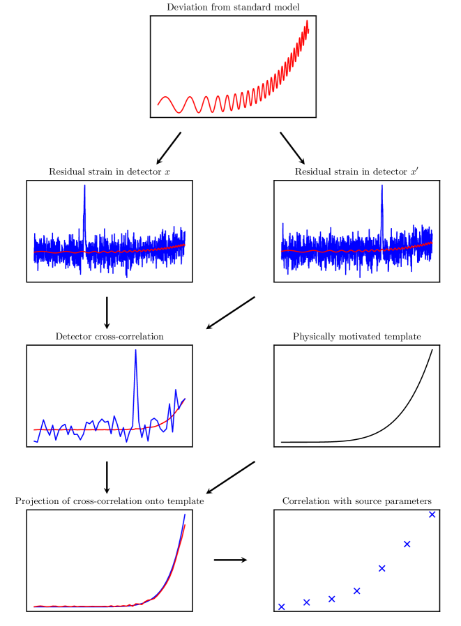
Figure 1: Outline of the SCoRe method. When a BM signature (in red) is measured by a pair of GW detectors, each detector will add onto it a different noise. The resulting residual strains, computed by subtracting the best-fit SM waveform from the data, are plotted in blue. Noise that is uncorrelated between detectors will be reduced when taking the cross-correlation between the two detectors. Higher power transient noise and correlated noise may remain, but can be mitigated by projecting CRPS onto some physically motivated template. Most BM signature models have a dependence on the source parameters. The projection coefficients measured over events of different source parameters may reveal such correlation.

II Motivation behind SCoRe

The search for BM physics using GWs is challenging due to multiple reasons, including both theoretical and experimental limitations. On one side, we are limited by the number of theoretical waveforms needed to test for the vast range of potentially BM scenarios (either for missing physics within GR, or sufficiently generic and complete waveforms beyond it). On the other side, we are limited by our understanding of the instrument noise properties when differentiating any BM signature from noise artifacts. Thus, often one fits the data with available waveform models to infer the best-fit source parameters and searches for any coherent residual signal [69, 70, 71, 5, 72]. However, the limitation remains in how well a framework can identify a BM signature and what the appropriate metric to quantify a deviation is. An example of this is the uneven performance of specific tests with different events (e.g. [8]).

A few salient features expected from any BM signature(s) in the GW data are (i) BM signatures will be common in the data of multiple detectors, but uncorrelated detector noise will not, (ii) a large class (if not all) of BM signatures can be understood as additional loss/gain in the orbital energy of a coalescing binary (e.g. [73, 7, 74, 75]) when compared to the SM (GR, and sources involving black holes and/or neutron stars) , (iii) BM signatures can depend on the GW source properties.

In this work, we propose a new technique to search for BM signatures in GW data that aims to address the issues mentioned above. This method has three key characteristics, each exploiting and/or targeting the three of BM signatures listed previously: (i) the residual GW data obtained after subtracting a modeled GW signal for a given waveform and source parameters are cross-correlated within pairs of detectors –to help distinguish signal from noise; (ii) the CRPS is projected on a physically motivated template. This template is either composed of the derivatives of the orbital frequency up to order $n$ (for a model-independent search), or derived from a particular physical model (for a model-dependent search) –to help characterize the signal; (iii) the projection is estimated as a function of the GW best-fit source parameters from the signal after marginalizing its uncertainties.

The first step helps in mitigating the contribution from uncorrelated noise to the residual signal by cross-correlating a total of $N_{\rm det}(N_{\rm det}-1)/2$ pairs of detectors, where $N_{\rm det}$ is the number of detectors. Cross-correlation is a useful tool technique to search for weak signals from noisy GW data and is often used to search for stochastic GW background signals  [56, 57]. It is a time averaging over the product of the strains in two different detectors. Because the noise at the two detectors is not correlated, its mean average is zero, and its standard deviation decreases as the timescale of integration is increased. A price is paid however for this noise reduction: features shorter than the averaging timescale will be lost. The second step aids to look for a physics-driven BM signal in either a model-dependent or a model-independent way. Projecting onto template functions also further reduces noise by filtering particular, model-motivated, structures in the signal. We suggest templates that are naturally expressible in terms of the orbital frequency. The final step takes into account possible dependencies of the BM signal on the GW source parameters and can also mitigate uncertainties related to the source parameters.

Although the idea of using template functions in frequency space is similar to the frames used in the BayesWave framework [76, 77] (which can also be used as template functions in SCoRe), our method does not seek to reproduce the residual signal with a set of functions. This is unlike current residual tests that use BayesWave [72, 5]. Instead, we measure the degree to which a pre-determined finite set of functions can explain the residual strain. This makes SCoRE morphology-dependent, but the morphology of the chosen template functions is arbitrary and can be non-specific. For example, one could reproduce the deviations parameters used in parametrized tests [6, 78, 79, 72], but choosing an agnostic template set using SCoRe is also possible, as we will explain in Sec III.2.

By using cross-correlation and projection onto a template, we hope to reduce noise well below that of individual detectors. With this noise reduction, SCoRe may be able to unearth minute BM signatures, which would otherwise remain undetected by only considering the strain of individual detectors. By looking at the structure of the CRPS, the method can help constrain potential deviations with a vast range of possible forms. This also means that the search for potential deviations can be made tighter as their form is guided with theoretical work. Furthermore, the method can also probe for correlations between the BM signature and the GW source parameters. A schematic diagram illustrating the basic principles of this technique is depicted in Fig. 1.

III Formalism for SCoRe

We describe below the formalism of SCoRe, which consists of four parts, (A) Cross-correlation, (B) Choice of a residual template, (C) Projection on a template, and (D) Inference using a Bayesian framework. We can write a linear model of the GW data $d^{x}(t)$ in a detector denoted by $x$ as

$$\begin{split}d^{x}(t)=&s^{x}(t)+n^{x}(t),\\ \end{split}$$ (1)

where $s^{x}(t)=\sum_{i}F^{x}_{i}(t)h_{i}(t)$ denotes the observed GW signal as seen by a detector, written in terms of the actual signal $h_{i}(t)$ for the polarization state “$i$”, and the corresponding detector response function $F^{x}_{i}$(t). The noise in detector $x$ is $n^{x}(t)$. Whether a signal is detected in a particular detector depends on the noise in the detector and the detector response function $F^{x}_{i}$(t) to the source position. In this work, we consider that a GW signal detected with a SM template in multiple detectors with a matched filtering SNR $\rho$ greater than a minimum threshold network SNR $\rho_{*}$ is classified as an event. Performing parameter estimation over the strains in the detector network gives a posterior over the source parameters $\theta$. By definition, the Maximum Likelihood Estimate (MLE), $\theta_{\text{MLE}}$, corresponds to the minimum residual strain amplitude in comparison to the variance in the detector noise, as $\theta_{\text{MLE}}$ should maximize the likelihood.

We propose to perform the test of BM physics on the residual data which is constructed using the MLE parameters inferred using a network of detectors, $\theta_{\text{MLE}}$ as

$$\begin{split}\Delta d_{\theta_{\text{MLE}}}^{x}(t)=&s(t)-s_{BF}(t)+n^{x}(t),\\ =&\Delta s(t)+n^{x}(t),\end{split}$$ (2)

where $s_{BF}(t)$ is the SM waveform for $\theta_{\text{MLE}}$. The MLE parameters need not be the true parameters of the source parameters—they only resemble the data best given a waveform model and the assumption of the standard model. Since such parameters will be generically described with a distribution, we introduce in Sec. III.4 a Bayesian framework to marginalize their (posterior) distribution.

III.1 Cross-correlation of the residual signal

One of the key aspects of a BM signature in the residual data is that it is likely to be correlated in all the detectors. However, it will be observed differently in each detector depending on the detector response function. Noise between multiple GW detectors from unrelated sources will be random. To identify the origin of the residual as either astrophysical (a BM signature) or due to detector noise, we propose to do a cross-correlation of the residual signal between the data from two detectors. Given the output $d^{x}(t)$ and $d^{x^{\prime}}(t)$ of two detectors $x$ and $x^{\prime}$, the general cross-correlation $Y(\tau)$ of the two signals over a timescale $\tau$ is defined as

$$Y(\tau)$$

$$\equiv\frac{1}{\tau}\int_{t-\tau/2}^{t+\tau/2}dt_{1}\int_{t-\tau/2}^{t+\tau/2}dt_{2}d^{x}(t_{1})d^{x^{\prime}}(t_{2})Q(t_{1},t_{2}),$$ (3)

where $Q(t_{1},t_{2})$ is a filter function. The choice of $\tau$ should balance two effects: correlated noise is reduced better as $\tau$ increases, but averaging washes away signal features with timescale shorter than $\tau$. In the limit where $\tau$ spans the length of the signal, the cross-correlation becomes the total residual power observed. There are natural choices of $\tau$, which rely on maximizing SNR while ensuring the features of the signal are preserved. They will depend on the source parameters, most importantly the chirp mass, which sets the timescale of the orbital frequency evolution, and the choice of template function on which to project the CRPS. We discuss the methodology behind choosing $\tau$ with a specific example in Sec. IV.2.

The definition (III.1) has been used to search for stochastic GW signal [56, 57]. There, the strain in multiple detectors is used to search for a common, periodic signal  [80]. In stochastic GW background searches, the phase of the signal is not expected to be resolved. This makes choosing the optimal filter function non-trivial. By contrast, we can measure the phase of a well-detected event and measure $\Delta t$, the delay time separating the two detectors within a timing uncertainty. The optimal filter function, which gives the highest SNR, will correspond to the signals in the detectors overlapping in time. It is therefore $Q(t_{1},t_{2})=\delta(|t_{1}-t_{2}|-\Delta t)$ (assuming $\tau\gg\Delta t$). We can then define the cross-correlation with maximum SNR with angular brackets:

$$\begin{split}&\left\langle d^{x}(t)d^{x^{\prime}}(t+\Delta t)\right\rangle\\ &\equiv\frac{1}{\tau}\int_{t-\tau/2}^{t+\tau/2}dt^{\prime}d^{x}(t^{\prime})d^{x^{\prime}}(t^{\prime}+\Delta t),\end{split}$$ (4)

and, more specifically, the cross-correlation of the residual strains:

$$\begin{split}D^{xx^{\prime}}(t)\equiv&\langle\Delta d_{\theta_{\text{MLE}}}^{x}(t)\Delta d_{\theta_{\text{MLE}}}^{x^{\prime}}(t+\Delta t)\rangle,\\ =&\langle\Delta s^{x}_{\theta_{\text{MLE}}}(t)\Delta s^{x^{\prime}}_{\theta_{\text{MLE}}}(t+\Delta t)\rangle+\langle n^{x}(t)n^{x^{\prime}}(t+\Delta t)\rangle.\end{split}$$ (5)

The value of $\Delta t$ will depend on the source parameters such as the sky position and also on the position of the two GW detectors $x$ and $x^{\prime}$ between which the signal is correlated. This can be inferred for individual pairs of detectors, and need not be assumed in the analysis. The detection of the correlated signal $D(t)$ depends on the overlap of the signal $\Delta s^{x}_{\theta_{\rm MLE}}(t)$ between the individual detectors, which depends on the response functions of the detectors $F_{i}^{x}$(t). We can marginalize over the response functions and extrinsic source parameters, as explained in Sec. III.4, so that we may account for different residual signatures that will be induced by the same BM deviation in different detectors. But, if, for a given antenna pattern, a theory predicts no measurable residual signature in multiple detectors, then the cross-correlation will not yield anything.

Using the cross-correlation definition given in Eq. (4), we can model the measured cross-correlated signal as

$$D^{xx^{\prime}}(t)=S^{xx^{\prime}}_{\theta_{\text{MLE}}}(t)+\mathcal{N}^{xx^{\prime}}_{c}(t),$$ (6)

where the first term denotes the correlated signal between the two detectors and the second term denotes the correlated residual noise between the two detectors. We usually assume that the noise between detectors is uncorrelated. In reality, some noise, like magnetic noise, can be correlated. Though these types of noise are unlikely to be dominant, they will play a role at some level in the mean, and their impact on the signal should be estimated when this technique is applied to the data.

If the noise is uncorrelated between the two detectors, then the second term in Eq. (6) vanishes and only the first term is non-zero. As a result, we can write

$$D^{xx^{\prime}}(t)= \langle\Delta s^{x}_{\theta_{\text{MLE}}}(t)\Delta s^{x^{\prime}}_{\theta_{\text{MLE}}}(t+\Delta t)\rangle$$

$$+\langle n^{x}(t)n^{x^{\prime}}(t+\Delta t)\rangle\delta_{xx^{\prime}}.$$ (7)

Alternatively, one can work in the time-frequency domain using the short-time Fourier transforms of the strains $s^{x}(t)$ and $s^{x^{\prime}}(t)$ and substituting in Eq. (4). The timescale used to compute the short-time Fourier transform should not be greater than the timescale of cross-correlation $\tau$. In the remaining analysis, for concreteness, we will work in the time domain.

III.2 Choice of residual Templates

The second “key-physics”-driven aspects that we want to explore in CRPS signals is that there might be more energy injection/extraction from a binary system in BM scenarios than in the SM templates. This difference in power released results, in particular, in a change in the orbital frequency evolution $f(t)$. Previous residual tests, such as the ones using BayesWave [76, 77], have proposed to decompose residual signals in terms of frames that have a natural expression in the frequency domain (Morlet-Gabor sine-Gaussian wavelets and “chirplets” [76]). Along similar arguments, we propose to decompose the CRPS signal into a template of $n$ orbital frequency-dependent functions $Z_{i}(f(t))$, which can capture any gain/loss in the (radiated) energy of the binary source after taking into account the dependence on the source parameters

$$S^{xx^{\prime}}_{\theta_{\text{MLE}}}(t)=\sum_{i=1}^{i=n}\alpha_{i}(\theta_{\text{MLE}},t)Z_{i}(f(t)),$$ (8)

where the (real) coefficients $\alpha_{i}$ may depend on the source parameters and time. These coefficients vanish when no BM signature is present in the data. Either side of the equation is valued in strain squared and will depend on the integration timescale $\tau$. The only requirement on the set of templates $Z_{i}(f(t))$ is that its elements should not be parallel to one another. They need not be either normalized or orthogonal. For example, one could choose wavelets or chirplets. Notice that one can also model the BM signature in terms of the residual strain of the GW signal rather than the power. As one still uses the CRPS to extract posterior information in either approach, they will yield the same information. We describe the strain modeling in Appendix A.

The specific form of the template functions $Z_{i}(f(t))$ can be motivated by a particular type of BM signature if such knowledge is available. As an alternative to choosing a specific, model-dependent set of template functions, we present a choice of template that we argue allows for an unmodeled BM search. The unmodeled template is constructed from the following observation: BM effects modify the rate of energy dissipation. This in turn impacts the rate at which orbital frequency increases. We thus expect the derivatives of the orbital frequency of the system to be good tracers of a BM signature.

More specifically, to capture the proportional change in time of the orbital frequency, we use the derivatives of $\dot{f}/f$ as our template functions

$$Z_{i>0}(t) =\left\langle\left(\frac{d^{i}\ln f(t)}{dt^{i}}\right)^{2}\right\rangle,$$ (9)

while $Z_{0}(t)$ is constant, defined to capture any BM signature with constant power. The template functions take values at bin positions. If the template functions are defined as functions of continuous time, one can simply take the angular bracket, as defined in Eq. (4), to define the expected CRPS functions.

We note that for inferring the values of $\alpha_{i}$ from data, it is convenient to orthogonalize and normalize the template functions, e.g. using the Gram-Schmidt process, if possible. If the physical interpretation of the coefficients is easier in the original form, then one can always transform the functions and their coefficients back.

III.3 Projection on a template

The projection of the CRPS of the data onto the chosen template encodes how well the model matches the signal. In this subsection, we define the projection coefficients and the associated uncertainty. The projection coefficient $\Gamma_{i}(D)$ of the CRPS signal $D^{xx^{\prime}}(t)$ onto the template $Z_{i}$ is:

$$\Gamma_{i}(D) =\int^{t_{e}}_{t_{s}}dtD^{xx^{\prime}}(t)Z_{i}(f(t)),$$ (10)

($t_{s}$, $t_{e}$ are the start/end of the signal in the data). Then, the requirement that the template functions should not be parallel is

$$Z_{i}-\Gamma_{i}(Z_{j})\tilde{Z}_{i}\neq 0\,\forall\,\{j\neq i\}\in n,$$ (11)

where $\tilde{Z}_{i}$ is normalized, so $\Gamma_{i}(\tilde{Z}_{i})=1$. The templates can be made orthonormal, that is $\Gamma_{i}(Z_{i})=1$ and $\Gamma_{i}(Z_{j})=\delta_{ij}$, if required for the inference of the signal. If an orthonormal set is chosen, then the projection coefficient $\Gamma_{i}(S)$ will be equal to $\alpha_{i}$. This is possible as long as the template functions are not linearly dependent. In the rest of this work, we will assume that the $Z_{i}$ used are orthonormal and hence the value of $\alpha_{i}$ is measured as the mean value of the projection of the data onto the template functions.

When measuring the CRPS and the coefficients, we will need to know the associated uncertainty. In this work, we compute the standard deviation in the limit of small-signal (zero mean value). In the limit where the cross-correlation scale goes to zero, $\tau\rightarrow 0$, the noise on the cross-correlation estimator can be obtained as

$$K^{2}_{n}\equiv\langle(\Delta d^{x}(t)\Delta d^{x^{\prime}}(t+\Delta t))^{2}\rangle-D(t)^{2}.$$ (12)

Assuming that the noise in each detector is Gaussian, stationary, and uncorrelated, we can simplify the above expression as

$$\begin{split}K^{2}_{n}\equiv&\langle n^{x}(t)n^{x}(t)\rangle\langle n^{x^{\prime}}(t)n^{x^{\prime}}(t)\rangle,\\ =&N^{2}_{x}N^{2}_{x^{\prime}},\end{split}$$ (13)

where in the second line we have defined the noise auto-correlation of each detector as $N^{2}_{x}$.

If there are no BM signatures present in the data, then the value of the coefficients $\alpha_{i}$ should be consistent with zero. However, in the case of a non-zero signal, we can write the estimator $\hat{\alpha}_{i}$ from the data. Assuming $\alpha_{i}$ does not depend on time, then we can write it in terms of the CRPS $D(t)$, the template functions $Z_{i}(f(t))$, and the noise on the CRPS, $K_{n}$, as

$$\begin{split}\hat{\alpha}^{xx^{\prime}}_{i}(\theta_{\text{MLE}})&=\int_{t_{s}}^{t_{e}}dtW_{i}(t)D^{xx^{\prime}}(t)Z_{i}(f(t)),\\ \text{where\,}W_{i}(t)&\equiv\frac{K^{-2}_{n}(t)}{\int_{t_{s}}^{t_{e}}K^{-2}_{n}(t)Z_{i}^{2}(f(t))dt}.\end{split}$$ (14)

In the above equation, $W_{i}(t)$ are weights which serve two purposes: (i) they ensure that the equation is normalized, and (ii) they account for any variation in the noise properties in the detector by inverse noise weighting. This helps in reducing the uncertainty in the estimator. For the situation of uncorrelated stationary Gaussian noise considered in this analysis, the values of $W_{i}(t)$ will be constant and will simply normalize $Z_{i}(t)$. However if the noise power spectral density (PSD) across a data segment shows variation with time $N_{x}^{2}(t)$ (non-stationarity), then $W_{i}(t)$ will not be a constant. If the $Z_{i}(f(t))$ are not orthogonal, $\hat{\alpha}_{i}$ will generally be non-zero even when $D(t)=Z_{j}(t)$, for $j\neq i$.

Finally, it is of interest to estimate the signal-to-noise ratio (SNR) for measuring the parameters $\hat{\alpha}$. For $N_{GW}$ sources with GW similar source parameters and with $N_{\rm det}$ GW detectors, we can write the combined SNR, $\rho_{i}$, as

$$\rho_{i}=\bar{\alpha}_{i}(\theta_{\text{MLE}})\times\bigg{[}\sum^{N_{\rm det}}_{x=1,x^{\prime}>x}\sum^{N_{GW}}_{j}{{(K^{xx^{\prime}}_{\alpha_{i}})}^{-2}}\bigg{]}^{1/2},$$ (15)

where, $\bar{\alpha}_{i}(\theta_{\text{MLE}})$ is the mean value of the inferred signal for all the detectors pairs and sources, and $(K^{xx^{\prime}}_{\alpha_{i}})^{2}$ is the noise on the parameter $\alpha_{i}$, defined as

$$(K^{xx^{\prime}}_{\alpha_{i}})^{2}=\int_{t_{s}}^{t_{e}}dt\left(W(t)K_{n}Z_{i}(t)\right)^{2}.$$ (16)

From the expression given in Eq. 15, we can conclude that the total SNR $\rho$ to measure a deviation $\alpha_{i}$ scales as $\sqrt{N_{GW}}$ and $\sqrt{N_{\rm det}(N_{\rm det}-1)/2}$. Finally it is important to clarify that the value of $\alpha$ can explicitly depend on the value of the source parameters $\{\theta_{\text{MLE}}\}$, and in that case so will the number of GW sources $N_{GW}(\theta_{\text{MLE}})$ with the best-fit source parameter $\theta_{\text{MLE}}$ that needs to be combined to obtain the SNR.

III.4 Inference using the Bayesian framework

In this section we formulate a hierarchical Bayesian framework to measure the presence of any BM signature in the observed data by marginalizing over the uncertainties associated with the GW source parameters. Let us denote $\mathcal{M}_{\text{SM}}$ as the SM, and $\Delta_{M}$ as a set of parameters which captures deviations from this model. Then, we can write the posterior distribution $\mathcal{P}(\Delta_{M}|\{d^{x}(t)\})$ on the parameters $\Delta_{M}$ given the observed set of data $\{d^{x}(t)\}$ detected at detectors labelled $x$ using Bayes’ theorem [81] as

$$\mathcal{P}(\Delta_{M}|\{d^{x}(t)\})\propto p(\{d^{x}(t)\}|\Delta_{M})\Pi(\Delta_{M}),$$ (17)

where $p(\{d^{x}(t)\}|\Delta_{M})$ denotes the likelihood and $\Pi(\Delta_{M})$ denotes the prior. For a set of $N_{\rm obs}$ independent events of GW sources detected (denoted by $\mathcal{S}$) above a matched filtering SNR $\rho_{*}$, we can simplify the likelihood as

$$\begin{split}&p(\{d^{x}(t)\}|\Delta_{M})\\ =&\prod^{N_{\rm det}}_{x,x^{\prime}>x=1}\prod_{i=1}^{N_{\rm obs}}p(\{d^{x},d^{x^{\prime}}\}_{i}|\mathcal{S},\Delta_{M})\\ =&\prod^{N_{\rm det}}_{x,x^{\prime}>x=1}\prod_{i=1}^{N_{\rm obs}}\frac{p(\mathcal{S}|\{d^{x},d^{x^{\prime}}\}_{i},\Delta_{M})p(\{d^{x},d^{x^{\prime}}\}_{i}|\Delta_{M})}{p(\mathcal{S}|\Delta_{M})},\end{split}$$ (18)

where in the third line, the first term denotes the probability of detecting events in the data given a small variation in the model $\Delta_{M}$, and the second term $p(\{d^{x},d^{x^{\prime}}\}_{i}|\Delta_{M})$ is the likelihood. We can write the likelihood including the GW source parameters $\theta$ with a prior $\Pi(\theta)$, and the dependence of any deviation on the GW source parameter, $p(\Delta_{M}|\theta)$, as

$$p(\{d^{x},d^{x^{\prime}}\}_{i}|\Delta_{M})=\int d\theta p(\{d^{x},d^{x^{\prime}}\}_{i}|\theta,\Delta_{M})p(\Delta_{M}|\theta)\Pi(\theta).$$ (19)

The term in the denominator in Eq. 18 is the evidence, which we can write in terms of the all possible events which are detectable above a matched filtering SNR $\rho_{*}$ as

$$p(\mathcal{S}|\Delta_{M})$$

$$=\int_{\rho\geq\rho_{*}}d\{d^{x}(t)\}\int d\theta p(\{d^{x}(t)\}|\theta,\Delta_{M})p(\Delta_{M}|\theta)\Pi(\theta).$$ (20)

If the detector noise is not changing with time, then the term $p(\{d^{x}(t)\}|\theta,\Delta_{M})$ will not vary with time and only depend on the detectability of an event above $\rho_{*}$, which we usually denote by $p_{\rm det}(\theta,\Delta_{M})$. If we assume, any signal with a matched filtering SNR above $\rho_{*}$ is detected, then Eq. (18) further simplifies. The term $\int p(\mathcal{S}|\{d^{x},d^{x^{\prime}}\}_{i},\Delta_{M})$ becomes unity. Putting all of this together, we can write the posterior on the parameters $\Delta_{M}$ as

$$\begin{split}\mathcal{P}(\Delta_{M}|&\{d^{x}(t)\})=\Pi(\Delta_{M})\times\\ &\prod^{N_{\rm det}}_{x,y>x=1}\prod_{i=1}^{N_{\rm obs}}\frac{\int p(\{d^{x},d^{x^{\prime}}\}_{i}|\theta,\Delta_{M})p(\Delta_{M}|\theta)\Pi(\theta)d\theta}{p(\mathcal{S}|\Delta_{M})}.\end{split}$$ (21)

This is the most general hierarchical Bayesian framework to search for a BM signature marginalizing over the source parameters uncertainties. In this analysis, we perform the Bayesian estimation on the residual signal obtained around a set of best-fit model parameters $\theta_{\rm BF}$ assuming $\mathcal{M}_{SM}$ as the SM. This allows us to define the deviation $\Delta_{M}$ as a function of $\theta_{\text{BF}}$ so we may check any correlation between BM signature and source parameters. Searches around the best-fit can also help in reducing the computational cost in performing the Bayesian analysis. However, the analysis pipeline can be easily modified to include the full Bayesian framework. The above equation around a best-fit value can be simplified into

$$\mathcal{P}(\alpha| \{d(t)\})=\Pi(\alpha)\prod^{N_{\rm det}}_{x=1,y>x}\prod_{i=1}^{N_{\rm obs}}\frac{\int p(\{d^{x},d^{x^{\prime}}\}_{i}|s(\theta_{\rm MLE}),\alpha)p(\alpha|\theta_{\rm MLE})p(\theta_{\rm MLE})d\theta_{\text{MLE}}}{p(\mathcal{S}|\alpha)},$$ (22)

where, $s(\theta_{\rm BF})$ is the GW signal for the set of best-fit parameters, $p(\theta_{\rm BF})$ is the posterior on the best-fit parameters obtained from the data assuming the SM, and $\alpha$ is the set of template coefficients for $\Delta_{M}$. The likelihood $p(\{d^{x},d^{x^{\prime}}\}_{i}|s(\theta_{\rm BF}),\alpha)$ can be written in terms of the CRPS as

$$\begin{split}p(\{d^{x},d^{x^{\prime}}\}_{i}|s(\theta_{\rm BF}),\alpha)=p(D(t)|\alpha).\end{split}$$ (23)

If we further assume the likelihood to be Gaussian and there is no correlated noise, then it becomes

$$\begin{split}&p(\{d^{x},d^{x^{\prime}}\}_{i}|s(\theta_{\rm BF}),\alpha)\\ &\propto\exp\bigg{(}-\int dt\frac{(D(t)-S_{\theta_{\text{MLE}}}(\alpha))^{2}}{2K_{n}^{2}(t)}\bigg{)},\end{split}$$ (24)

where $D(t)$ can be calculated using Eq. (III.1) and the noise covariance matrix can be calculated using Eq. (12). In the presence of correlated noise $\mathcal{N}_{c}$ it can be included in the noise covariance matrix.

Though this method can detect the presence of any kind of BM signature in the GW data, model-independent searches may fail to completely capture the structure of the deviation if the chosen template only partially overlaps with the BM signature. However, using the Bayesian framework proposed here, one can do a Bayesian model comparison for different BM scenarios and perform a tuned search for the model with higher Bayesian evidence.

IV Application of SCoRe on a toy example for an unmodeled search

We now illustrate the SCoRe method by using the unmodeled power template to recover a toy model injection from simulated data. We describe the toy model, then discuss the appropriate choice of cross-correlation timescale. Using the SCoRe framework, we finally recover the injected value in the simulated data and perform the Bayesian analysis described in Sec. III.4.

IV.1 Generating mock data

As a toy model on which to apply this template, we create simulated mock data by adding Gaussian noise realisations $n^{x}$ over a simulated strain $s(t)$ as

$$d^{x}(t)=s(t)+n^{x}(t).$$ (25)

The strain is $s(t)\equiv s_{\text{SM}}(t)+\Delta s_{\text{BM}}$; it includes a standard model signal $s_{\text{SM}}(t)$ and a BM signal $\Delta s_{\text{BM}}$. The BM signal is modeled as $\Delta s_{\text{BM}}(t)=b\frac{d\ln f_{\text{SM}}(t)}{dt}$, with $b$ as a free parameter that controls the strength of the BM signal. The standard model waveform is the same for all events. It is computed using LALSuite [82] called through PyCBC [83] and the IMRPhenomD approximant [84, 85] for an equal mass, non-spinning, circular BBH merger, at a luminosity distance of $100$ Mpc and the individual masses are both set to $m=5M_{\odot}$. A sampling rate of $16384$Hz is used throughout this work. Both cross- and plus-polarizations are used to derive $f_{\text{SM}}$. The plus-polarization is used as the standard model signal $s_{\text{SM}}$. We assume Gaussian, stationary noise and the same sensitivity for all detectors. Different events in each of the two distinct detectors are then simulated by drawing realisations $n^{x}$ of the expected O4 noise sensitivity [86].

We project the CRPS onto the unmodeled template given in (9). In the rest of the work, we implement the angular bracket average of Eq. (4) as a binned mean. Out of the template terms given in Eq. (9), we only use the linear term $Z_{1}$. The toy model with the BM signal $\Delta s_{\text{BM}}$ is constructed such that it perfectly overlaps with the template $Z_{1}$ to show how the recovery can happen for the best case scenario. We expect that the template coefficient $\alpha_{1}$ can recover the injected BM signal $\Delta s_{\text{BM}}$ completely. Certainly, in reality different BM theories will only have a partial projection on the template, unless one performs a model-dependent search. In the future, we will explore different choices of template to illustrate how they can project onto different BM theories. Theoretical efforts to produce waveforms in some such theories have been presented in e.g. [74, 87] and so have their impact data analysis in modeled and unmodeled searches e.g. [88, 9].

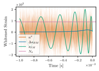
Figure 2: Example toy model data. We use the PyCBC software package to generate $s_{\text{SM}}$, the waveform for a circular, non-spinning, equal mass BBH, with individual masses both equal to $5M_{\odot}$. This is plotted in green. We add onto it a BM signature, $\Delta s_{\text{BM}}$ (blue line), that is proportional to the change in the orbital frequency logarithm ($\tilde{\alpha}_{1}=0.05$). It is normalized so that, for $\tilde{\alpha}_{1}=1$, the maximum amplitude reaches to the noise auto-correlation, $N_{x}$ (purple line). Realisations of Gaussian, stationary noise are added to $s_{\text{SM}}+\Delta s_{\text{BM}}$ to obtain different events. Some examples of noise realisations are plotted in orange.

.

We generate $N_{\text{GW}}$ pairs of strain data as in Eq. (25) and attribute each of these strains to one of the two detectors $x$ or $x^{\prime}$. Examples of each of the components used to construct these data are shown in Fig. 2. We assume that the best fit parameters are known exactly, and that they are those used to generate $s_{\text{SM}}(t)$. We therefore subtract $s_{\text{SM}}$ from each of these strains to obtain $\Delta d^{x,x^{\prime}}$. In real data, the error from estimating $\theta_{\text{MLE}}$ needs to be accounted for both in the residual strains and in the template and we need to perform the marginalization described in Sec. III.4.

Each pair of $\Delta d^{x,x^{\prime}}$ is then cross-correlated as in Eq. (5) to obtain the CRPS, $D^{x,x^{\prime}}_{i}$, where $i$ labels events. We obtain $N_{\text{GW}}$ residual time series that, for real data, would each be associated with a GW event. Examples of the CRPS are shown by orange lines in Fig. 3. An estimator $\hat{\alpha}_{1}$ is obtained for each of these time-series by projecting onto the template according to Eq. (14). It is convenient to define the dimensionless quantities

$$\begin{split}\tilde{Z}_{1}&=P^{-1}Z_{1},\quad\text{such that}\int_{t_{\text{s}}}^{t_{\text{e}}}\tilde{Z}_{1}^{2}dt=1,\\ \tilde{\alpha}_{1}&=\frac{\alpha_{1}}{\alpha^{0}_{1}},\quad\alpha_{1}^{0}=\frac{PN_{x}^{2}}{\text{max}\left(\frac{d\ln f}{dt}\right)^{2}},\end{split}$$ (26)

where $\alpha^{0}_{1}$ is defined so that, when the maximum amplitude of $\Delta s_{\text{BM}}$ is $N_{x}$, the projection of its cross-correlation onto $\tilde{Z}_{1}$ is $\tilde{\alpha}_{1}=1$. The normalization constant, $P$, is a measure of the mean power per bin in the template function. During this procedure, the timescale $\tau$ over which the residual strains are cross-correlated is a free parameter. We discuss the choice of $\tau$ in the next subsection.

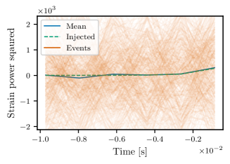
Figure 3: Residual data and injected BM signature cross-correlated over $\tau=1.28\times 10^{-3}$ s. The blue line is the mean of the CRPS over 500 events, plotted in orange. It corresponds to the MLE value of $\tilde{\alpha}_{1}$ when projected onto the template. The dashed green line is the cross-correlation of $\Delta s_{\text{BM}}$.

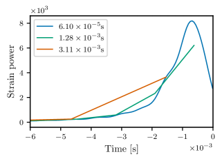
Figure 4: Cross-correlation template $\tilde{Z}_{1}$ for different cross-correlation timescales $\tau$. The smallest timescale allowed by the sampling rate, $\tau=6.10\times 10^{-5}$ s, has features that are washed away as the timescale is increased. With $\tau\in[0.8,1.6]\times 10^{-3}s$, no new physical features appear and information remains the same as $\tau$ is increased. For timescales longer than $2.1\times 10^{-3}$ s, all the power is effectively concentrated in a single bin.

IV.2 Choice of $\tau$

When $\tau$ is finite, the noise on the cross-correlation estimator, in the limit of a small signal is

$$K^{2}_{D} =\frac{1}{n_{\text{window}}}K^{2}_{n},$$ (27)

where $n_{\text{window}}$ is the number of data points measured in the timescale $\tau$. The advantage of taking the mean over a timescale $\tau$ is that $K_{D}\propto 1/\tau$, so, in the limit of large $\tau$, the cross-correlation tends to be the residual signal (and correlated noise). On the other hand, as mentioned, some information is lost in the averaging over the timescale $\tau$. This is illustrated in Fig. 4. The cross-correlation template $\tilde{Z}_{1}$ is computed from $s_{\text{SM}}$ with different values of $\tau$. As $\tau$ is increased, the shape of $\tilde{Z}_{1}$ is qualitatively changed. By integrating over $\tau$, we lose the ability to differentiate between BM models that give different template predictions below this timescale.

For a specific template, two choices of $\tau$ have equivalent signal content if no new physical behavior arises at an intermediate timescale. If they are equivalent, the average power per bin, $P$, will be the same. This quantity is plotted in Fig. 5 as a function of $\tau$. For this example, at timescales shorter than $0.8\times 10^{-3}$ s, the mean power decreases as the “pulse” feature of the template seen in Fig. 4 is integrated out. For $\tau\in[0.8,1.6]\times 10^{-3}$ s, the mean power remains constant as the template functions resemble power laws and a smaller $\tau$ does not add information. An example of a template with a timescale in this range is shown by the green line in Fig. 4 (obtained by averaging over $\tau=1.28\times 10^{-3}$ s). When averaging over timescales larger than $\tau\sim 2.1\times 10^{-3}$ s, all the power of the BM signature is concentrated in a single bin. Past this point, the mean power per bin, $P$ scales as $\left(\tau\right)^{-1/2}$.

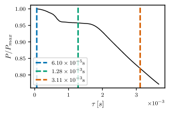
Figure 5: Template normalization factor (mean power per bin $P$) as $\tau$ is increased. The template with $\tau=6.10\times 10^{-5}$ s contains a pulse. As the pulse is washed away by the averaging, the mean power per bin decreases. Between $0.8\times 10^{-3}s<\tau<1.6\times 10^{-3}s$, averaging over a greater $\tau$ does not change the shape of the template and the mean power remains constant. At scales greater than $2.1\times 10^{-3}$ s a single bin contains the majority of the power and the mean power scales as $\tau^{-1/2}$.

This exact evolution sequence of the mean power per bin $P$ as a function of $\tau$ is specific to our chosen template (9) and the standard model waveform used for the computation. However, the criteria that can be used to choose $\tau$ will be the same in all cases.

The first natural choice of $\tau$ corresponds to the maximum SNR, which is achieved when most of the power is concentrated in as small a bin as possible. This is determined by the $\tau$ where the mean power per bin, $P$, starts scaling as $\tau^{-1/2}$. This may not, however, correspond to the highest Bayes factor in favor of a BM.

If information about the structure of the BM signal is preferred over a higher SNR, then $\tau$ should be accordingly chosen. In our toy model, for our specific choice of template and SM waveform, to conserve information about the “chirp” part of the template, the $\tau$ value needs to be set to the rightmost point on the horizontal section of the $P$ shown in Fig. 5, $\tau=1.8\times 10^{-3}$ s. In this case, it is not possible to preserve information about the pulse shape while still taking the cross-correlation, as one would need to set $\tau$ to the sampling interval. It may yet be possible to keep some benefits of taking the cross-correlation while not averaging over the pulse shape by letting the averaging timescale vary with time. For example, we may set $\tau$ to 1 over the sampling rate from $t=-10^{-3}$ s to $t=0$, and set $\tau\in(0.8,1,6)\times 10^{-3}$ s for $t\in(-5,-1)\times 10^{-3}$ s to maximise noise reduction over the “chirp”. Finally, we could average the rest of the time domain, where the CRPS is dominated by noise, into one bin ( $t=(t_{\text{s}},-5)\times 10^{-3}$ s).

In this section, we consider only a time-constant $\tau$, which we set to the SNR-maximising value, $\tau=1.8\times 10^{-3}$ s. The cross-correlations plotted in Fig. 3 are computed over this timescale. This choice of $\tau$ is specific to this template function and best-fit source parameters, as the variation of the mean power $P$ with $\tau$ will change for other choices of template and source parameters. Since the templates depend on the orbital frequency, we expect the choice of $\tau$ to vary (scale) with chirp mass for all choices of templates.

IV.3 Bayesian inference of the injected signal

In this section, we use the Bayesian framework presented in Sec. III.4 to combine events into one measurement of $\tilde{\alpha}_{1}$. We assume the source parameters are perfectly known to be $\tilde{\theta}_{\text{BF}}$. Therefore, $p(\tilde{\theta}_{\text{BF}})=\delta(\theta_{\text{MLE}}-\tilde{\theta}_{\text{BF}})$, where $\delta(x)$ is the Dirac delta function. This assumption is made to show how this new method will work in the best-case scenarios. In reality, each estimated parameter will have an error, and one can marginalize the uncertainty as presented in Sec. III.4. Furthermore, since we assume $\alpha_{1}$ is unique for the given source parameters, $p(\alpha_{1}|\tilde{\theta}_{\text{BF}})=1$. The posterior on $\tilde{\alpha}_{1}$ is then

$$\begin{split}\mathcal{P}&\left(\tilde{\alpha}_{1}|\{d(t)\}\right)\\ &\propto\Pi(\tilde{\alpha}_{1})\exp\left(-\frac{1}{2\tilde{K}^{2}_{\tilde{\alpha}}}\left(\tilde{\alpha}_{1}-\tilde{\alpha}_{1,MLE}\right)^{2}\right),\end{split}$$ (28)

where $\tilde{\alpha}_{1,MLE}=1/(N_{\text{GW}}\alpha_{1}^{0})\sum^{N_{\text{GW}}}_{i}\int^{t_{\text{e}}}_{t_{\text{s}}}\tilde{Z}_{1}D_{i}dt$, and

$$\tilde{K}_{\tilde{\alpha}_{1}}^{2}=\frac{K^{2}_{\alpha_{1}}}{\left(a_{1}^{0}\right)^{2}N_{\text{GW}}}.$$ (29)

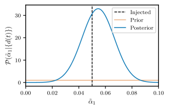
Figure 6: Posterior on $\tilde{\alpha}_{1}$ for $N_{\text{GW}}=500$, when the template function $Z_{1}$ is injected in Gaussian, stationary noise. We used a flat prior from $0$ to $1$, giving a Bayes factor of $773$. The error on $\tilde{\alpha}$ is $\tilde{K}_{\tilde{\alpha}}$, the SNR for this measurement is 4.5.

The likelihood is thus a Gaussian distribution with Maximum Likelihood Estimator (MLE) $\tilde{\alpha}_{1,\text{MLE}}$ and variance $\tilde{K}^{2}_{\tilde{\alpha}_{1}}$. With our assumption, the MLE is the mean over events of the estimator $\hat{\alpha}_{1}$. Since the projection is linear, it corresponds to the projection of the mean CRPS, shown in blue in Fig. 3.

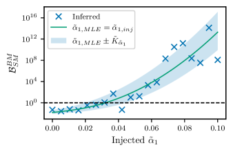
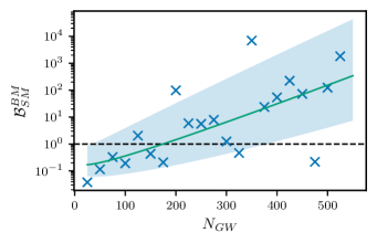
Figure 7: Bayes factor $\mathcal{B}^{\text{BM}}_{\text{SM}}$ in favor of a BM hypothesis over the standard model hypothesis left for different values of $\tilde{\alpha}_{1,\text{inj}}$ ($N_{\text{GW}}=500$), right for different $N_{\text{GW}}$ ($\tilde{\alpha}_{1,\text{inj}}=5\times 10^{-2}$). The solid green line indicates the case of perfect accuracy as a guide. The blue region covers one $\tilde{K}_{\alpha}$ deviations in the measured value of $\tilde{\alpha}_{\text{1,MLE}}$. The standard model waveform used is that of an equal mass BBH with individual mass $5M_{\odot}$.

If a signal is correlated between detectors, its cross-correlation $S^{xx^{\prime}}(t)$ must be positive. Our template function is positive, therefore so must be $\alpha_{1}$ and $\tilde{\alpha}_{1}$. We choose a flat prior on $\tilde{\alpha}_{1}$ ranging from 0 to $\tilde{\alpha}_{1,max}$, so that $\Pi(\tilde{\alpha}_{1})=\left(\tilde{\alpha}_{1,max}\right)^{-1}$. The posterior obtained from the events in Fig. 3, which have injection $\tilde{\alpha}_{1}=0.05$, is shown is shown in Fig. 6. The prior used is set with $\tilde{\alpha}_{1,max}=1$.

With this posterior, we can compare the standard model hypothesis with the hypothesis of a BM signature by computing $\mathcal{B}^{\text{BM}}_{\text{SM}}$, the Bayes factor in favor of a BM signature being present as opposed to just the SM. Since the standard model is recovered when the coefficient $\alpha_{i}$ is zero, we compute $\mathcal{B}^{\text{BM}}_{\text{SM}}$ as the Savage-Dickey density

$$\mathcal{B}^{\text{BM}}_{\text{SM}} =\frac{\Pi(0)}{P(\tilde{\alpha}_{1}=0|\{d(t)\})},$$ (30)

which can be computed directly in our toy model, since the analytical form of the posterior in terms of $\tilde{\alpha}_{1,MLE}$, $K^{2}_{D}$, and $N_{\text{GW}}$ is known. In fact, the expression for $\mathcal{B}^{\text{BM}}_{\text{SM}}$ can be written explicitly in terms of error functions

$$\begin{split}\mathcal{B}^{\text{BM}}_{\text{SM}}&=\sqrt{\frac{\pi}{2}}\frac{\tilde{K}_{\tilde{\alpha}_{1}}}{\tilde{\alpha}_{1,\text{max}}}\exp\left(-\frac{1}{2}\left(\frac{\tilde{\alpha}_{1,\text{MLE}}}{\tilde{K}_{\tilde{\alpha}_{1}}}\right)^{2}\right)\times\\ &\left(\text{erf}\left(\frac{\tilde{\alpha}_{1,\text{MLE}}}{\sqrt{2}\tilde{K}_{\tilde{\alpha}_{1}}}\right)-\text{erf}\left(\frac{\tilde{\alpha}_{\text{MLE}}-\tilde{\alpha}_{1,\text{max}}}{\sqrt{2}\tilde{K}_{\tilde{\alpha}_{1}}}\right)\right),\end{split}$$ (31)

where $c=(1/2)\tilde{K}^{2}_{\tilde{\alpha}_{1}}$ and $\text{erf}(x)=(2/\sqrt{\pi})\int^{x}_{0}\exp\left(-y^{2}\right)dy$. This can be computed numerically. We plot the dependence on $N_{\text{GW}}$ and on the injected value of $\tilde{\alpha}_{1}$ in green on Fig. 7, assuming a perfectly accurate measurement ($\tilde{\alpha}_{1,MLE}=\tilde{\alpha}_{1,\text{inj}}$). In the left plot, the number of events is kept fixed at $N_{\text{GW}}=500$ as the injected value of $\tilde{\alpha}_{1}$ is varied, while on the right plot, $N_{\text{GW}}$ is varied as $\tilde{\alpha}_{1,\text{inj}}$ is kept fixed. We also plot values of $\tilde{\alpha}_{1,MLE}$ measured from realizations of the toy model data with crosses.

The value of $\Pi(0)$ can significantly change the recovered value of the Bayes factor. This is a manifestation of Occam’s penalty [89]: a wider prior compared to the likelihood indicates a more constraining underlying hypothesis. The prior we choose has $\tilde{\alpha}_{1,max}=1$. This maximum prior is quite large ($1\gg\tilde{\alpha}_{1}+\tilde{\Sigma}_{\tilde{\alpha}_{1}}$), and reducing it can increase the Bayes factor obtained without truncating most of the area under the likelihood. However, we choose it on physical grounds, as we assume any yet undetected BM signature has to be smaller than the noise variance.

V Application of SCoRe on a beyond GR model

V.1 Toy model EFT and numerical set-up

To explore our method in a realistic scenario –including inspiral, merger and ringdown– we construct a waveform model that captures key effects expected from an effective field theory (EFT) extension of General Relativity under the assumption that the coupling scale is of the order (or below) that of the BH scale. The model accounts for: (i) higher curvature corrections in the inspiraling regime can be captured at leading order by tidal effects, (ii) the merger transitions to a post-merger regime described by quasinormal modes for the black hole described by such a theory and, importantly, that corrections scale with the mass of the system appropriately. To fix ideas, and choose a convenient scaling so its dependence is sufficiently marked, we envision our system described by a Lagrangian ${\cal L}=R+{l}^{4}{\cal L}_{(6)}$, where ${\cal L}_{(6)}$ indicates the higher order corrections to the curvature, scaling in this example as $M^{-4}$ (see e.g. [91, 92, 93, 94]). For modeling the merger, we follow [95] and construct an interpolating signal between inspiral and ringdown guided by the behavior of null geodesics corresponding to the final black hole. The main characteristics (mass and spin) of such a final black hole can be estimated using a strategy similar to that given in [96, 97] as long as the general solution for a rotating black hole in a given theory is known. For the inspiral regime, we use a simple effective one-body EOB model [98] with tidal interactions as in [99] (see also  [100]) transitioning to the final black hole at the innermost stable circular orbit (ISCO) frequency of the final black hole. For concreteness, we focus on the equal mass, non-rotating, binary black holes with no eccentricity.  Importantly, we note that for the theories described by the above Lagrangian, closed-form solutions are only known for slowly (or non) rotating scenarios while the merger outcome should yield a black hole with spin $a/M\approx 0.67$ –with a small correction that also scales as $M^{-4}$. Without such a solution, the specific value of such correction can not be computed yet. However, we note that this correction is quite smaller than the correction to the horizon area (e.g. [92]) and so black hole compaction is more affected than associated quasinormal modes. Last, gravitational radiation from this theory can be captured to leading order by the correction to the Quadrupole of the system; its associated effect, in turn, can be accounted for in the stationary phase approximation to the waveform as discussed in [90]. Combining the above information, we “phenomenologically” account for dynamical departures in the theory by extrapolating from the slowly rotating case with the following assignments:

$$C=\frac{1}{2}-\frac{5}{16}\epsilon\,,\,k^{T}=\frac{1008}{25}\epsilon\,,\,$$ (32)

$$\delta\omega^{R}_{\mbox{QNM}}/{}^{GR}\omega^{R}_{\mbox{QNM}}=1+0.45\epsilon,$$ (33)

$$\delta\omega^{I}_{\mbox{QNM}}/{}^{GR}\omega^{I}_{\mbox{QNM}}=1-2.75\epsilon,$$ (34)

with $C$ the compaction of each black hole, $k^{T}$ the tidal Love number, $\delta\omega$ the correction to QNMs and where $\epsilon=(M_{*}/M_{T})^{4}$ and $M_{*}$ a base scale which we take to be $=M_{\odot}=1.5$ km. That is, the EFT is such that it assumes corrections to General Relativity, become ${\cal O}(1)$ at such length, thereby affecting the inspiral only at a subtle level.

V.2 Choice of template

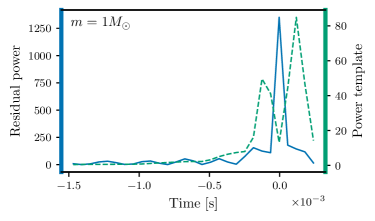
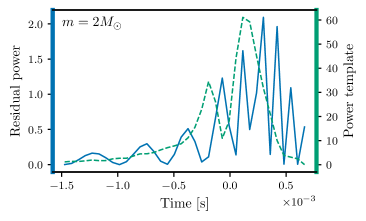
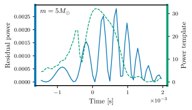
Figure 8: Residual power and template functions. The residual signals are obtained from subtracting the GR waveforms from the EFT waveforms with the same source parameters. They are plotted with blue, solid lines (left axis). The template functions $\tilde{Z}_{1}$ are computed from the GR signal using a value of $\tau$ equal to the sampling interval. They are plotted with dotted green lines (right axis). The template in Eq. (9) is unmodeled, and is not expected to match actual signal at finite order, but it does capture the time interval over which the most power is present.

We perform the same analysis as in Sec. IV on the NR waveforms motivated by the EFT. The strain signal $s(t)$ is now the full numerical waveform obtained with the source at $d_{l}=100$ Mpc. We assume that the standard waveform corresponding to the best-fit parameters, $s_{\text{SM}}(t)$, is the NR waveform obtained with the same source parameters in GR. These correspond to equal mass, non-spinning, quasi-circular black hole binaries with individual masses given by $m/M_{\odot}=1,2~{}~{}\mbox{and}~{}~{}5.$

In Sec. IV, the BM signature introduced was directly proportional to the template function, $Z_{1}$. As described in Sec. III, more realistic residual signals such as the one obtained from the EFT-inspired waveform will require a possibly infinite number of higher-order terms to be accurately described. The first order (normalized) template function $\tilde{Z}_{1}$ obtained from the GR waveforms using $\tau$ equal to the sampling interval is plotted for different $m$ with dotted lines in Fig. 8. The power of the residual strains is plotted with full blue lines. Although the template functions do not track the short-scale time evolution, they do capture the time interval over which residual power is present.

To choose the timescale over which to cross-correlate, we note that the power templates have two peaks. Ideally, one would integrate over the smaller feature seen in the template—in this case, the narrower of the peaks in power. This would be the feature seen around $-0.2$ to 0 milliseconds for $m=1M_{\odot}$, $-0.4$ to 0 milliseconds for $m=2M_{\odot}$, and from $-0.6$ to $0.2$ milliseconds for $M=5M_{\odot}$. However, for $m=1M_{\odot}$ and $2M_{\odot}$, at the maximum currently available sampling rate ($16384$Hz), the residual power signals only span 2-5 sample points. We therefore choose to lose precision in favor of a higher SNR: averaging over both peaks (up to the value of $\tau$ at which the mean power per bin $P$ scales as $\tau^{-1/2}$), which gives the highest SNR. This corresponds to integrating from around $-0.25$ to $0.25$ milliseconds and from $-0.5$ to 0.5 milliseconds for $m=1M_{\odot}$ and $2M_{\odot}$, respectively. For $m=5M_{\odot}$, the larger peak is smoother. As a result, integrating over both peaks (for example, from $-1$ to 1 milliseconds) does not give a larger SNR. For all masses, lower values of $\tau$ lead to a decrease in SNR.

The values of $\tau$ chosen for each mass are shown in Table 1. The coefficients obtained by projecting the residual power onto the template with the aforementioned values of $\tau$ are also shown in the table.

V.3 Recovery of injected signal

The values of $\tilde{\alpha}_{1}$ corresponding to the injected residual power are plotted with green crosses in Fig. 9. The values recovered from toy data with $N_{\text{GW}}=500$ are plotted with blue discs and error bars. For $m=2$ and $5$ M_⊙, the recovered values are consistent with zero in comparison to the standard deviation $\tilde{K}_{\tilde{\alpha}_{1}}$, as indicated by a downward arrow on the error bars.

$\frac{m}{M_{\odot}}$	$\tau$ (s)	$\tilde{\alpha}_{1,\text{inj}}$	$\tilde{\alpha}_{1,MLE}$	SNR	$\mathcal{B}^{\text{BM}}_{\text{SM}}$	FAR
1	$4.27\times 10^{-4}$	$7.20\times 10^{-2}$	$1.02\times 10^{-1}$	3.05	8.69	$1.6\times 10^{-3}$
2	$1.22\times 10^{-3}$	$2.22\times 10^{-4}$	$1.66\times 10^{-2}$	0.60	0.06	$2.7\times 10^{-1}$
5	$1.22\times 10^{-3}$	$1.78\times 10^{-7}$	$5.47\times 10^{-3}$	0.46	0.02	$3.2\times 10^{-1}$

Table 1: Projection coefficients of the injected BM signal and the recovered maximum likelihood estimation (MLE) of the NR EFT waveforms for $500$ events. The values of $\tau$ are chosen so that the SNR is maximized and the smallest scale feature captured. They depend on the best-fit waveform. The drop in Bayes factor from $m=1M_{\odot}$ to $m=2,5M_{\odot}$ is due to the mean recovered value of $\tilde{\alpha}_{1}$ moving within error range of $\tilde{\alpha}_{1}=0$. The False Alarm Rate (FAR) is computed as the probability of obtaining a value equal or larger than the $\tilde{\alpha}_{1}$ measured when there is no signal in the data (see Appendix B) for a Gaussian stationary noise.

In this particular BM model, the power of the residual signal decreases with mass as $m^{-8}$. Regardless of the template chosen, the projection of the residual power onto it will also scale as $m^{-8}$. This is the case for the injected values of $\tilde{\alpha}_{1}$. The dotted orange line corresponds to a fit though these points with gradient $m^{-8}$—the template functions correctly capture the scaling of the NR waveform residuals. The fact that the template functions correctly capture the timescale and the power scaling of the BM signature is not trivial, as they are agnostic to the model and were not informed about the nature of the EFT used to simulate the NR waveforms. This is one of the salient aspect of the method SCoRe. For $m=2$ and $5$ M_⊙, $\tilde{\alpha}_{1,\text{inj}}\ll\tilde{K}_{\tilde{\alpha}}$. The Bayes factor for both these masses is inconsequential, and we cannot recover the scaling with mass.

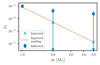
Figure 9: Injected and recovered values of $\tilde{\alpha}_{1}$. The projections of the actual residual signal on $Z_{1}$ are shown with green crosses. They correctly scale as $m^{-8}$, shown by the orange dotted line. The blue discs are values measured from toy data constructed with $500$ events. The error $\tilde{K}_{\tilde{\alpha}}$, shown by the error bars is several orders of magnitude larger than the injected values for $m=2$ and $5$ M_⊙. The measurements for these masses are consistent with zero, as indicated by the downward porting arrows, and the scaling with $m$ cannot be recovered.

We have assumed that the only term scaling with the source parameter we are investigating, which is mass in this example, is due to the BM signature, so that the residual strain scales with a power $k$, where $k$ captures the dependence of the BM signal, on the source parameters $\theta$ as $\Delta d\propto\theta^{k}$. For the EFT model considered here, $k=-4$ and $\theta$ is the source mass. In reality, the residual strain may contain contributions from unaccounted BM physics, waveform systematics, or a stealth bias, for example. These contributions may scale with the same source parameter as the BM signature, but with a different dependence, such as $\theta^{k^{\prime}}$. Then depending on the value of $k^{\prime}$ relative to $k$ and the range over which the value of $\theta$ is observed, one may still fail to recover the scaling with $k$ even with large network SNR and $\tilde{K}_{\tilde{\alpha}}\ll\tilde{\alpha}_{1,\text{inj}}$. In the case of a stealth bias, we would naïvely assume $k^{\prime}=-4$. This is because, as the magnitude of the BM signature changes, so will the magnitude of its projection onto the SM manifold. More complicated dependence on the source parameters of the BM signature may yet arise, as noted in [64].

VI Conclusion and future outlook

In this work we propose a new method, SCoRe, to search for BM signatures in GW data by projecting the cross-correlated residual power spectrum signal on a theory-independent or theory-dependent template, which can capture a large class of BM scenarios and its dependence on the GW source parameters.

As one of the key features of BM signatures is that they will be universal in all the detectors, cross-correlating between different pairs helps mitigate contamination from uncorrelated noise artifacts in the BM signal. Correlated and strong transient noise, as well as any unmodeled BM physics, will not be reduced by cross-correlation. To account for this, the second step of the SCoRe method is to project the cross-correlated residual power onto a template capturing a specific frequency dependence. This frequency dependence can be tuned for both modeled and unmodeled searches. An expected facet of BM signatures, however, is that they can be understood as a change in the orbital energy radiated by the coalescing binary. As an alternative to modeled searches, we therefore also propose to search for dependence on the derivatives of the logarithm of orbital frequency as a tracker of energy radiated per orbit.

Many BM signatures are expected to vary as a function of the source parameters. The final step of the SCoRe method is to check for correlation between the projection coefficients measured and the values of the best-fit parameters used to compute the residuals. We incorporated a hierarchical Bayesian framework for the marginalization of source parameters (around a best-fit value) of multiple events of the cross-correlation signal obtained by combining all possible pairs of GW detectors.

For the unmodeled searches, the template may not be able to completely capture the deviation from the standard model, however, it can indicate signatures of possible deviations from the standard model. To understand which BM scenarios best explain the data, one can do a Bayesian model comparison. This can be incorporated into the framework proposed in this work. Following that a model-dependent search using the template choice which is tuned for the BM scenario which shows maximum Bayesian evidence in the unmodeled search can be performed.

To illustrate our method, we have applied it to a toy model and also to waveforms motivated by an EFT of gravity [91, 92, 93, 94]. In both cases, the injected residual power was mainly concentrated in the last few milliseconds (before the peak of the waveform) of a signal and the noise was Gaussian, stationary, and colored according to the expected O4 PSD.

For the toy model, we showed how well different signal strengths could be recovered, as measured by the Bayes factor in favor of the presence of a BM signature, for different levels of power injected and number of events combined. The events used all had the same source parameters. Crucially, they were all at a luminosity distance $d_{l}$ of $100$ Mpc. In reality, sources are expected to be distributed over a large range of luminosity distances, in which case the residual power will scale as $d_{l}^{-2}$. In addition, since the properties of the source and their astrophysical population will critically impact the Bayes factors recovered, we will work next on taking into account astrophysical populations to obtain more realistic estimates on how well the method can infer the presence and structure of BM signatures.

The illustration of the method on the EFT-motivated NR waveforms constrained the BM signatures around zero and could not detect the injected signatures for the masses giving the smallest residual power ($m=2,5M_{\odot}$). However, the model-independent template we suggest for agnostic searches was successful in capturing the time range over which most of the residual power was emitted. It could also correctly infer the minute BM signal for $m=M_{\odot}$. As this search is performed using a model-independent template, it could not reproduce the exact structure of the residual signal, as expected. In this scenario, we suggest that, once one has identified a promising result using the model-independent search, the templates should be refined. This can either be done by using a model-dependent templates or by adding higher-order derivatives to the model-independent template functions.

This work has been to present the main lines of the SCoRe method. One of the main caveat of our results is that they assume Gaussian, stationary noise. Although these assumptions are used in the LVK analyses [2, 3, 4], we are working on applying this method on the GW data available to investigate the effect of realistic noise, and what the FAR for different templates may be. We will also consider, in future work, how transient noise (glitches) affects the recovery of BM signals from data.

We hope that SCoRe will not only be useful to search for signatures of new physics, but also a large class of scenarios within the standard model ranging from unmodeled GR effects to deviation in the waveform due to waveform modeling systematics.

We have illustrated the method with toy models in this work and will, in future works, provide tests and predictions for its applications. We will explore the capability of this technique in recovering different scenarios and the corresponding appropriate template banks which can be useful to search for both modeled and unmodeled searches.

Appendix A Modeling residual strain

In Sec. III.2, we have discussed the template constructed to recover signal from the cross-correlation power spectrum. In this section, we will briefly describe the template that can be used to model any deviation on the strain. Instead of modeling the residual power, $\mathcal{S}_{\theta}(t)$, we can model the residual strain $\Delta s_{\theta}$. In that case, the above equations written for $\mathcal{P}_{\theta}(t)$ will only get a minor modification. The decomposition of the signal in terms of template functions (Eq. (8)) becomes

$$\Delta s_{\theta_{\text{MLE}}}(t)=\sum_{i=1}^{i=n}\beta_{i}(\theta_{\text{MLE}})\zeta_{i}(f(t)),$$ (35)

where the coefficients $\beta{i}$ and bases $\zeta_{i}$ give $\alpha_{i}$ and $Z_{i}$ when cross-correlated using Eq. (4). In this case, both sides of the equation still depend on the timescale $\tau$, but they take values in strain rather than strain power.

In analogy to Eq. (14), we can write the estimator for $\beta$ as

$$\hat{\beta}_{i}(\theta_{\text{MLE}})=\int_{t_{s}}^{t_{e}}dtW_{i}(t)D(t)^{1/2}\zeta_{i},$$ (36)

with $W_{i}(t)=K^{-1}_{n}(t)/\int_{t_{s}}^{t_{e}}K^{-1}_{n}(t)\zeta_{i}(t)^{2}dt$. The corresponding SNR is

$$\rho_{i}^{2}=\sum^{N_{\rm det}}_{x=1,x^{\prime}>x}\sum^{N_{GW}}_{j}\left(\frac{(\hat{\beta}^{xx^{\prime}}_{i}(\theta_{\text{MLE}}))^{2}}{{(K^{xx^{\prime}}_{\beta_{i}})}^{2}}\right)_{j},$$ (37)

where, ${(K^{xx^{\prime}}_{\beta_{i}})}^{2}$ is the noise on the parameter $\beta$ is defined as

$${(K^{xx^{\prime}}_{\beta_{i}})}^{2}=\int_{t_{s}}^{t_{e}}dt\left(W_{i}(t)K_{n}^{\frac{1}{2}}\zeta_{i}(t)\right)^{2},$$ (38)

where there is now a square root on $K_{n}$.

Again for a Gaussian, stationary, uncorrelated noise, we will get a $\sqrt{N_{GW}}$ enhancement in the SNR by combining $N_{\text{GW}}$ events and number of detector pairs $\sqrt{N_{\rm det}(N_{\rm det}-1)/2}$.

Appendix B False Alarm Rate

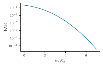
Figure 10: False alarm rate (FAR) on the measurement of $\alpha$ for Gaussian, stationary noise. We define the FAR for a value of the projection coefficient $\alpha$ as the probability of obtaining a measurement equal or greater to $\alpha$ from data without a signal. Since our noise is Gaussian and stationary, this is given by the survival function of a Gaussian distribution. Here, we plot the survival function for the normal distribution, which gives the FAR as a function of the ratio of $\alpha$ to the error on $\alpha$.

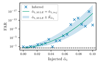
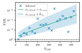
Figure 11: False Alarm Rate (FAR), or the probability of measuring a projection coefficient equal or greater to $\tilde{\alpha}_{1}$ . The y-axis scale has been inverted to show that the FAR scales in the same way as $\mathcal{B}_{\text{SM}}^{\text{BM}}$, the Bayes factor in favor of a BM hypothesis, shown in Fig. 7. The dashed line is a visual aid indicating a FAR of 0.5.

The False Alarm Rate (FAR) is a measure of the probability of detecting a signal when it is absent from the data. In the LVK catalogs [2, 3, 4], the FARs reported are computed using real data and using different methods depending on the pipeline used. In this work, we define the FAR for a given value of $\alpha$ to be the probability of obtaining a value of $\alpha$ equal or greater when there is no signal in the data. As we are considering Gaussian, stationary noise, the (frequentist) distribution of $\alpha$ measurements from noise is a Gaussian distribution centred around zero, with variance given by Eq. (16). The FAR is then the survival function of this Gaussian evaluated at $\alpha$:

$$\text{FAR}(\alpha) =1-\int^{\alpha}_{-\infty}d\alpha\frac{1}{K_{\alpha}\sqrt{2\pi}}\exp\left(-\frac{1}{2}\left(\frac{\alpha}{K_{\alpha}}\right)^{2}\right)$$

The FAR for any pair of measured $\alpha$ and $K_{\alpha}$ can be obtained by substituting $\alpha/K_{\alpha}$ in the survival function for the normal distribution, plotted in Fig. 10. The same can be done with $\tilde{\alpha}_{1}/\tilde{K}_{\alpha}$.

The FAR scales with the injected projected coefficient and the number of events in the same way as the Bayes factor, as shown in Fig. 11. In future work, we will compute the FAR by considering available GW data and how often an event that is not believed to contain any BM signal can lead to a non-zero measurement of the projection coefficients.

References

- B. P. Abbott et al. (2016a) [LIGO Scientific and Virgo Collaborations] B. P. Abbott et al. (LIGO Scientific and Virgo Collaborations), Observation of Gravitational Waves from a Binary Black Hole Merger, Physical Review Letters 116, 061102 (2016a).
- B. P. Abbott et al. (2019a) [LIGO Scientific and Virgo Collaborations] B. P. Abbott et al. (LIGO Scientific and Virgo Collaborations), GWTC-1: A Gravitational-Wave Transient Catalog of Compact Binary Mergers Observed by LIGO and Virgo during the First and Second Observing Runs, Physical Review X 9, 031040 (2019a), arXiv:1811.12907 .
- B. P. Abbott et al. (2021a) [LIGO Scientific and Virgo Collaborations] B. P. Abbott et al. (LIGO Scientific and Virgo Collaborations), GWTC-2: Compact Binary Coalescences Observed by LIGO and Virgo During the First Half of the Third Observing Run, Physical Review X 11, 021053 (2021a), arXiv:2010.14527 .
- B. P. Abbott et al. (2021) [LIGO Scientific, Virgo, and KAGRA Collaborations] B. P. Abbott et al. (LIGO Scientific, Virgo, and KAGRA Collaborations), GWTC-3: Compact Binary Coalescences Observed by LIGO and Virgo During the Second Part of the Third Observing Run, arXiv:2111.03606 (2021), arXiv:2111.03606 [astro-ph, physics:gr-qc] .
- B. P. Abbott et al. (2021) [LIGO Scientific, Virgo and KAGRA Collaborations] B. P. Abbott et al. (LIGO Scientific, Virgo and KAGRA Collaborations), Tests of General Relativity with GWTC-3 (2021), arXiv:2112.06861 [astro-ph, physics:gr-qc, physics:hep-th] .
- Agathos et al. [2014] M. Agathos, W. Del Pozzo, T. G. F. Li, C. Van Den Broeck, J. Veitch, and S. Vitale, TIGER: A data analysis pipeline for testing the strong-field dynamics of general relativity with gravitational wave signals from coalescing compact binaries, Physical Review D 89, 082001 (2014), arXiv:1311.0420 [astro-ph, physics:gr-qc] .
- Yunes and Pretorius [2009] N. Yunes and F. Pretorius, Fundamental Theoretical Bias in Gravitational Wave Astrophysics and the Parameterized Post-Einsteinian Framework, Phys. Rev. D 80, 122003 (2009), arXiv:0909.3328 [gr-qc] .
- Johnson-McDaniel et al. [2022] N. K. Johnson-McDaniel, A. Ghosh, S. Ghonge, M. Saleem, N. V. Krishnendu, and J. A. Clark, Investigating the relation between gravitational wave tests of general relativity, Phys. Rev. D 105, 044020 (2022), arXiv:2109.06988 [gr-qc] .
- Edelman et al. [2021] B. Edelman, F. J. Rivera-Paleo, J. D. Merritt, B. Farr, Z. Doctor, J. Brink, W. M. Farr, J. Gair, J. S. Key, J. McIver, and A. B. Nielsen, Constraining unmodeled physics with compact binary mergers from GWTC-1, Physical Review D 103, 042004 (2021).
- Hu and Veitch [2022] Q. Hu and J. Veitch, Accumulating errors in tests of general relativity with the Einstein Telescope: Overlapping signals and inaccurate waveforms (2022), arXiv:2210.04769 [astro-ph, physics:gr-qc] .
- Lyu et al. [2022] Z. Lyu, N. Jiang, and K. Yagi, Constraints on Einstein-dilation-Gauss-Bonnet gravity from Black Hole-Neutron Star Gravitational Wave Events, Physical Review D 105, 064001 (2022), arXiv:2201.02543 [astro-ph, physics:gr-qc] .
- Niu et al. [2021] R. Niu, X. Zhang, B. Wang, and W. Zhao, Constraining Scalar-tensor Theories Using Neutron Star–Black Hole Gravitational Wave Events, The Astrophysical Journal 921, 149 (2021).
- Pardo et al. [2018] K. Pardo, M. Fishbach, D. E. Holz, and D. N. Spergel, Limits on the number of spacetime dimensions from GW170817, Journal of Cosmology and Astroparticle Physics 2018 (07), 048.
- Nair et al. [2019] R. Nair, S. Perkins, H. O. Silva, and N. Yunes, Fundamental Physics Implications for Higher-Curvature Theories from Binary Black Hole Signals in the LIGO-Virgo Catalog GWTC-1, Physical Review Letters 123, 191101 (2019).
- Yunes et al. [2016] N. Yunes, K. Yagi, and F. Pretorius, Theoretical Physics Implications of the Binary Black-Hole Mergers GW150914 and GW151226, Physical Review D 94, 084002 (2016), arXiv:1603.08955 [astro-ph, physics:gr-qc, physics:hep-ph, physics:hep-th] .
- Kostelecký and Mewes [2016] V. A. Kostelecký and M. Mewes, Testing local Lorentz invariance with gravitational waves, Physics Letters B 757, 510 (2016).
- Mastrogiovanni et al. [2020] S. Mastrogiovanni, D. A. Steer, and M. Barsuglia, Probing modified gravity theories and cosmology using gravitational-waves and associated electromagnetic counterparts, Phys. Rev. D 102, 044009 (2020), arXiv:2004.01632 [gr-qc] .
- Okounkova et al. [2022a] M. Okounkova, W. M. Farr, M. Isi, and L. C. Stein, Constraining gravitational wave amplitude birefringence and Chern-Simons gravity with GWTC-2, Physical Review D 106, 044067 (2022a).
- Shao [2020] L. Shao, Combined search for anisotropic birefringence in the gravitational-wave transient catalog GWTC-1, Physical Review D 101, 104019 (2020).
- Abedi et al. [2017] J. Abedi, H. Dykaar, and N. Afshordi, Echoes from the abyss: Tentative evidence for Planck-scale structure at black hole horizons, Physical Review D 96, 082004 (2017).
- Ashton et al. [2016] G. Ashton, O. Birnholtz, M. Cabero, C. Capano, T. Dent, B. Krishnan, G. D. Meadors, A. B. Nielsen, A. Nitz, and J. Westerweck, Comments on: “Echoes from the abyss: Evidence for Planck-scale structure at black hole horizons” (2016), arXiv:1612.05625 [astro-ph, physics:gr-qc] .
- Uchikata et al. [2019] N. Uchikata, H. Nakano, T. Narikawa, N. Sago, H. Tagoshi, and T. Tanaka, Searching for black hole echoes from the LIGO-Virgo catalog GWTC-1, Physical Review D 100, 062006 (2019).
- Westerweck et al. [2018] J. Westerweck, A. B. Nielsen, O. Fischer-Birnholtz, M. Cabero, C. Capano, T. Dent, B. Krishnan, G. Meadors, and A. H. Nitz, Low significance of evidence for black hole echoes in gravitational wave data, Physical Review D 97, 124037 (2018).
- Will [1998] C. M. Will, Bounding the mass of the graviton using gravitational-wave observations of inspiralling compact binaries, Physical Review D 57, 2061 (1998).
- Belgacem et al. [2018a] E. Belgacem, Y. Dirian, S. Foffa, and M. Maggiore, The gravitational-wave luminosity distance in modified gravity theories, Physical Review D 97, 104066 (2018a), arXiv:1712.08108 [astro-ph, physics:gr-qc, physics:hep-th] .
- Belgacem et al. [2018b] E. Belgacem, Y. Dirian, S. Foffa, and M. Maggiore, Modified gravitational-wave propagation and standard sirens, Phys. Rev. D 98, 023510 (2018b), arXiv:1805.08731 [gr-qc] .
- Nishizawa [2018] A. Nishizawa, Generalized framework for testing gravity with gravitational-wave propagation. I. Formulation, Physical Review D 97, 104037 (2018).
- Mukherjee et al. [2021] S. Mukherjee, B. D. Wandelt, and J. Silk, Testing the general theory of relativity using gravitational wave propagation from dark standard sirens, Mon. Not. Roy. Astron. Soc. 502, 1136 (2021), arXiv:2012.15316 [astro-ph.CO] .
- Mewes [2019] M. Mewes, Signals for Lorentz violation in gravitational waves, Physical Review D 99, 104062 (2019).
- Mirshekari et al. [2012] S. Mirshekari, N. Yunes, and C. M. Will, Constraining Lorentz-violating, modified dispersion relations with gravitational waves, Physical Review D 85, 024041 (2012).
- O’Neal-Ault et al. [2021] K. O’Neal-Ault, Q. G. Bailey, T. Dumerchat, L. Haegel, and J. Tasson, Analysis of Birefringence and Dispersion Effects from Spacetime-Symmetry Breaking in Gravitational Waves, Universe 7, 380 (2021).
- Berti et al. [2006] E. Berti, V. Cardoso, and C. M. Will, Gravitational-wave spectroscopy of massive black holes with the space interferometer LISA, Physical Review D 73, 064030 (2006).
- Cardoso et al. [2016a] V. Cardoso, E. Franzin, and P. Pani, Is the Gravitational-Wave Ringdown a Probe of the Event Horizon?, Physical Review Letters 116, 171101 (2016a).
- Cardoso et al. [2016b] V. Cardoso, S. Hopper, C. F. B. Macedo, C. Palenzuela, and P. Pani, Gravitational-wave signatures of exotic compact objects and of quantum corrections at the horizon scale, Physical Review D 94, 084031 (2016b).
- Cardoso and Pani [2017] V. Cardoso and P. Pani, Tests for the existence of black holes through gravitational wave echoes, Nature Astronomy 1, 586 (2017).
- Gossan et al. [2012] S. Gossan, J. Veitch, and B. S. Sathyaprakash, Bayesian model selection for testing the no-hair theorem with black hole ringdowns, Physical Review D 85, 124056 (2012).
- Meidam et al. [2014] J. Meidam, M. Agathos, C. Van Den Broeck, J. Veitch, and B. S. Sathyaprakash, Testing the no-hair theorem with black hole ringdowns using TIGER, Physical Review D 90, 064009 (2014).
- Dreyer et al. [2004] O. Dreyer, B. Kelly, B. Krishnan, L. S. Finn, D. Garrison, and R. Lopez-Aleman, Black-hole spectroscopy: Testing general relativity through gravitational-wave observations, Classical and Quantum Gravity 21, 787 (2004).
- Mazur and Mottola [2004] P. O. Mazur and E. Mottola, Gravitational vacuum condensate stars, Proceedings of the National Academy of Sciences 101, 9545 (2004).
- Liebling and Palenzuela [2012] S. L. Liebling and C. Palenzuela, Dynamical Boson Stars, Living Reviews in Relativity 15, 6 (2012).
- Giudice et al. [2016] G. F. Giudice, M. McCullough, and A. Urbano, Hunting for Dark Particles with Gravitational Waves, Journal of Cosmology and Astroparticle Physics 2016 (10), 001, arXiv:1605.01209 [astro-ph, physics:gr-qc, physics:hep-ph] .
- Danielsson et al. [2021] U. Danielsson, L. Lehner, and F. Pretorius, Dynamics and Observational Signatures of Shell-like Black Hole Mimickers, Physical Review D 104, 124011 (2021), arXiv:2109.09814 [astro-ph, physics:gr-qc, physics:hep-th] .
- Eardley et al. [1973] D. M. Eardley, D. L. Lee, and A. P. Lightman, Gravitational-Wave Observations as a Tool for Testing Relativistic Gravity, Physical Review D 8, 3308 (1973).
- B. P. Abbott et al. (2019b) [LIGO Scientific and Virgo Collaborations] B. P. Abbott et al. (LIGO Scientific and Virgo Collaborations), Tests of General Relativity with GW170817, Physical Review Letters 123, 011102 (2019b).
- Yang et al. [2017] H. Yang, K. Yagi, J. Blackman, L. Lehner, V. Paschalidis, F. Pretorius, and N. Yunes, Black hole spectroscopy with coherent mode stacking, Phys. Rev. Lett. 118, 161101 (2017), arXiv:1701.05808 [gr-qc] .
- Zimmerman et al. [2019] A. Zimmerman, C.-J. Haster, and K. Chatziioannou, On combining information from multiple gravitational wave sources, Phys. Rev. D 99, 124044 (2019), arXiv:1903.11008 [astro-ph.IM] .
- V. Kalogera et al. [2021] V. Kalogera et al., The Next Generation Global Gravitational Wave Observatory: The Science Book (2021), arXiv:2111.06990 [gr-qc] .
- Barausse et al. [2020] E. Barausse et al., Prospects for Fundamental Physics with LISA, Gen. Rel. Grav. 52, 81 (2020), arXiv:2001.09793 [gr-qc] .
- B. P. Abbott et al. (2016b) [LIGO Scientific and Virgo Collaborations] B. P. Abbott et al. (LIGO Scientific and Virgo Collaborations), Characterization of transient noise in Advanced LIGO relevant to gravitational wave signal GW150914, Classical and Quantum Gravity 33, 134001 (2016b).
- B. P. Abbott et al. (2020a) [LIGO Scientific and Virgo Collaborations] B. P. Abbott et al. (LIGO Scientific and Virgo Collaborations), A guide to LIGO–Virgo detector noise and extraction of transient gravitational-wave signals, Classical and Quantum Gravity 37, 055002 (2020a).
- L. Blackburn et al. [2008] L. Blackburn et al., The LSC glitch group: Monitoring noise transients during the fifth LIGO science run, Classical and Quantum Gravity 25, 184004 (2008).
- Chatziioannou et al. [2019] K. Chatziioannou, C.-J. Haster, T. B. Littenberg, W. M. Farr, S. Ghonge, M. Millhouse, J. A. Clark, and N. Cornish, Noise spectral estimation methods and their impact on gravitational wave measurement of compact binary mergers, Physical Review D 100, 104004 (2019).
- R. Abbott et al. (2021) [LIGO Scientific and Virgo Collaborations] R. Abbott et al. (LIGO Scientific and Virgo Collaborations), Open data from the first and second observing runs of Advanced LIGO and Advanced Virgo, SoftwareX 13, 100658 (2021).
- Edy et al. [2021] O. Edy, A. Lundgren, and L. K. Nuttall, Issues of mismodeling gravitational-wave data for parameter estimation, Physical Review D 103, 124061 (2021).
- Kwok et al. [2022] J. Y. L. Kwok, R. K. L. Lo, A. J. Weinstein, and T. G. F. Li, Investigation of the effects of non-Gaussian noise transients and their mitigation in parameterized gravitational-wave tests of general relativity, Physical Review D 105, 024066 (2022).
- B. P. Abbott et al. (2004) [LIGO Scientific Collaboration] B. P. Abbott et al. (LIGO Scientific Collaboration), Analysis of first LIGO science data for stochastic gravitational waves, Physical Review D 69, 122004 (2004).
- Allen and Romano [1999] B. Allen and J. D. Romano, Detecting a stochastic background of gravitational radiation: Signal processing strategies and sensitivities, Physical Review D 59, 102001 (1999).
- Schumann [1952] W. O. Schumann, über die Dämpfung der elektromagnetischen Eigenschwingungen des Systems Erde — Luft — Ionosphäre, Zeitschrift für Naturforschung A 7, 250 (1952).
- P. Nguyen et al. [2021] P. Nguyen et al., Environmental noise in advanced LIGO detectors, Classical and Quantum Gravity 38, 145001 (2021).
- Thrane et al. [2013] E. Thrane, N. Christensen, and R. M. S. Schofield, Correlated magnetic noise in global networks of gravitational-wave detectors: Observations and implications, Physical Review D 87, 123009 (2013).
- Thrane et al. [2014] E. Thrane, N. Christensen, R. M. S. Schofield, and A. Effler, Correlated noise in networks of gravitational-wave detectors: Subtraction and mitigation, Physical Review D 90, 023013 (2014).
- Vallisneri and Yunes [2013] M. Vallisneri and N. Yunes, Stealth bias in gravitational-wave parameter estimation, Physical Review D 87, 102002 (2013).
- Vitale and Del Pozzo [2014] S. Vitale and W. Del Pozzo, How serious can the stealth bias be in gravitational wave parameter estimation?, Physical Review D 89, 022002 (2014).
- Okounkova et al. [2022b] M. Okounkova, M. Isi, K. Chatziioannou, and W. M. Farr, Gravitational wave inference on a numerical-relativity simulation of a black hole merger beyond general relativity (2022b), arXiv:2208.02805 [astro-ph, physics:gr-qc] .
- Ryan [1995] F. D. Ryan, Gravitational waves from the inspiral of a compact object into a massive, axisymmetric body with arbitrary multipole moments, Physical Review D 52, 5707 (1995).
- Poisson [1998] E. Poisson, Gravitational waves from inspiraling compact binaries: The quadrupole-moment term, Physical Review D 57, 5287 (1998).
- Laarakkers and Poisson [1999] W. G. Laarakkers and E. Poisson, Quadrupole Moments of Rotating Neutron Stars, The Astrophysical Journal 512, 282 (1999).
- Krishnendu et al. [2017] N. V. Krishnendu, K. G. Arun, and C. K. Mishra, Testing the Binary Black Hole Nature of a Compact Binary Coalescence, Physical Review Letters 119, 091101 (2017).
- B. P. Abbott et al. (2020b) [LIGO Scientific and Virgo Collaborations] B. P. Abbott et al. (LIGO Scientific and Virgo Collaborations), Properties and Astrophysical Implications of the 150 Binary Black Hole Merger GW190521, The Astrophysical Journal 900, L13 (2020b).
- B. P. Abbott et al. (2016c) [LIGO Scientific and Virgo Collaborations] B. P. Abbott et al. (LIGO Scientific and Virgo Collaborations), Tests of General Relativity with GW150914, Physical Review Letters 116, 221101 (2016c).
- B. P. Abbott et al. (2019c) [LIGO Scientific and Virgo Collaborations] B. P. Abbott et al. (LIGO Scientific and Virgo Collaborations), Tests of general relativity with the binary black hole signals from the LIGO-Virgo catalog GWTC-1, Physical Review D 100, 104036 (2019c).
- B. P. Abbott et al. (2021b) [LIGO Scientific and Virgo Collaborations] B. P. Abbott et al. (LIGO Scientific and Virgo Collaborations), Tests of General Relativity with Binary Black Holes from the second LIGO-Virgo Gravitational-Wave Transient Catalog, Physical Review D 103, 122002 (2021b), arXiv:2010.14529 .
- Damour and Esposito-Farese [1992] T. Damour and G. Esposito-Farese, Tensor multiscalar theories of gravitation, Class. Quant. Grav. 9, 2093 (1992).
- Barausse et al. [2013] E. Barausse, C. Palenzuela, M. Ponce, and L. Lehner, Neutron-star mergers in scalar-tensor theories of gravity, Phys. Rev. D 87, 081506 (2013), arXiv:1212.5053 [gr-qc] .
- Will [2014] C. M. Will, The Confrontation between General Relativity and Experiment, Living Rev. Rel. 17, 4 (2014), arXiv:1403.7377 [gr-qc] .
- Cornish and Littenberg [2015] N. J. Cornish and T. B. Littenberg, Bayeswave: Bayesian inference for gravitational wave bursts and instrument glitches, Classical and Quantum Gravity 32, 135012 (2015).
- Cornish et al. [2021] N. J. Cornish, T. B. Littenberg, B. Bécsy, K. Chatziioannou, J. A. Clark, S. Ghonge, and M. Millhouse, BayesWave analysis pipeline in the era of gravitational wave observations, Physical Review D 103, 044006 (2021).
- J. Meidam et al. [2018] J. Meidam et al., Parametrized tests of the strong-field dynamics of general relativity using gravitational wave signals from coalescing binary black holes: Fast likelihood calculations and sensitivity of the method, Physical Review D 97, 044033 (2018).
- Mehta et al. [2022] A. K. Mehta, A. Buonanno, R. Cotesta, A. Ghosh, N. Sennett, and J. Steinhoff, Tests of General Relativity with Gravitational-Wave Observations using a Flexible–Theory-Independent Method (2022), arXiv:2203.13937 [gr-qc] .
- Dhurandhar et al. [2008] S. Dhurandhar, B. Krishnan, H. Mukhopadhyay, and J. T. Whelan, Cross-correlation search for periodic gravitational waves, Phys. Rev. D 77, 082001 (2008), arXiv:0712.1578 [gr-qc] .
- Bayes and Price [1763] T. Bayes and n. Price, LII. An essay towards solving a problem in the doctrine of chances. By the late Rev. Mr. Bayes, F. R. S. communicated by Mr. Price, in a letter to John Canton, A. M. F. R. S, Philosophical Transactions of the Royal Society of London 53, 370 (1763).
- LIGO Scientific Collaboration [2018] LIGO Scientific Collaboration, LIGO Algorithm Library - LALSuite, free software (GPL) (2018).
- A. Nitz et al. [2022] A. Nitz et al., Gwastro/pycbc: V2.0.2 release of PyCBC, Zenodo (2022).
- Husa et al. [2016] S. Husa, S. Khan, M. Hannam, M. Pürrer, F. Ohme, X. J. Forteza, and A. Bohé, Frequency-domain gravitational waves from nonprecessing black-hole binaries. I. New numerical waveforms and anatomy of the signal, Physical Review D 93, 044006 (2016).
- Khan et al. [2016] S. Khan, S. Husa, M. Hannam, F. Ohme, M. Pürrer, X. J. Forteza, and A. Bohé, Frequency-domain gravitational waves from nonprecessing black-hole binaries. II. A phenomenological model for the advanced detector era, Physical Review D 93, 044007 (2016).
- B. P. Abbott et al. (2020) [LIGO Scientific, Virgo, and KAGRA Collaborations] B. P. Abbott et al. (LIGO Scientific, Virgo, and KAGRA Collaborations), Prospects for observing and localizing gravitational-wave transients with Advanced LIGO, Advanced Virgo and KAGRA, Living Reviews in Relativity 23, 3 (2020).
- Bernard [2018] L. Bernard, Dynamics of compact binary systems in scalar-tensor theories: Equations of motion to the third post-Newtonian order, Phys. Rev. D 98, 044004 (2018), arXiv:1802.10201 [gr-qc] .
- Sampson et al. [2014] L. Sampson, N. Yunes, N. Cornish, M. Ponce, E. Barausse, A. Klein, C. Palenzuela, and L. Lehner, Projected Constraints on Scalarization with Gravitational Waves from Neutron Star Binaries, Phys. Rev. D 90, 124091 (2014), arXiv:1407.7038 [gr-qc] .
- Isi et al. [2022] M. Isi, W. M. Farr, and K. Chatziioannou, Comparing Bayes factors and hierarchical inference for testing general relativity with gravitational waves (2022), arXiv:2204.10742 [astro-ph, physics:gr-qc] .
- Sennett et al. [2020] N. Sennett, R. Brito, A. Buonanno, V. Gorbenko, and L. Senatore, Gravitational-Wave Constraints on an Effective Field-Theory Extension of General Relativity, Phys. Rev. D 102, 044056 (2020), arXiv:1912.09917 [gr-qc] .
- de Rham et al. [2019] C. de Rham, L. Heisenberg, and A. J. Tolley, Spin-2 fields and the weak gravity conjecture, Phys. Rev. D 100, 104033 (2019), arXiv:1812.01012 [hep-th] .
- Cardoso et al. [2018] V. Cardoso, M. Kimura, A. Maselli, and L. Senatore, Black Holes in an Effective Field Theory Extension of General Relativity, Phys. Rev. Lett. 121, 251105 (2018), arXiv:1808.08962 [gr-qc] .
- Cano et al. [2022] P. A. Cano, K. Fransen, T. Hertog, and S. Maenaut, Gravitational ringing of rotating black holes in higher-derivative gravity, Phys. Rev. D 105, 024064 (2022), arXiv:2110.11378 [gr-qc] .
- Cayuso and Lehner [2020] R. Cayuso and L. Lehner, Nonlinear, noniterative treatment of EFT-motivated gravity, Phys. Rev. D 102, 084008 (2020), arXiv:2005.13720 [gr-qc] .
- McWilliams [2019] S. T. McWilliams, Analytical Black-Hole Binary Merger Waveforms, Phys. Rev. Lett. 122, 191102 (2019), arXiv:1810.00040 [gr-qc] .
- Buonanno et al. [2008] A. Buonanno, L. E. Kidder, and L. Lehner, Estimating the final spin of a binary black hole coalescence, Phys. Rev. D 77, 026004 (2008), arXiv:0709.3839 [astro-ph] .
- Kesden [2008] M. Kesden, Can binary mergers produce maximally spinning black holes?, Phys. Rev. D 78, 084030 (2008), arXiv:0807.3043 [astro-ph] .
- Buonanno and Damour [2000] A. Buonanno and T. Damour, Transition from inspiral to plunge in binary black hole coalescences, Phys. Rev. D 62, 064015 (2000), arXiv:gr-qc/0001013 .
- Hotokezaka et al. [2013] K. Hotokezaka, K. Kyutoku, and M. Shibata, Exploring tidal effects of coalescing binary neutron stars in numerical relativity, Physical Review D 87, 044001 (2013).
- Damour et al. [2012] T. Damour, A. Nagar, and L. Villain, Measurability of the tidal polarizability of neutron stars in late-inspiral gravitational-wave signals, Physical Review D 85, 123007 (2012).
- Bhat et al. [2022] S. A. Bhat, P. Saini, M. Favata, and K. G. Arun, Systematic bias on the inspiral-merger-ringdown consistency test due to neglect of orbital eccentricity (2022), arXiv:2207.13761 [astro-ph, physics:gr-qc] .
- C. R. Harris et al. [2020] C. R. Harris et al., Array programming with NumPy, Nature 585, 357 (2020).
- P. Virtanen et al. [2020] P. Virtanen et al., SciPy 1.0: Fundamental Algorithms for Scientific Computing in Python, Nature Methods 17, 261 (2020).
- Hunter [2007] J. D. Hunter, Matplotlib: A 2d graphics environment, Computing in Science & Engineering 9, 90 (2007).
- Waskom [2021] M. L. Waskom, Seaborn: Statistical data visualization, Journal of Open Source Software 6, 3021 (2021).