Extracting Wilson loop operators and fractional statistics from a
single bulk ground state
Abstract
An essential aspect of topological phases of matter is the existence of Wilson loop operators that keep the ground state subspace invariant. Here we present and implement an unbiased numerical optimization scheme to systematically find the Wilson loop operators given a single ground state wave function of a gapped Hamiltonian on a disk. We then show how these Wilson loop operators can be cut and glued through further optimization to give operators that can create, move, and annihilate anyon excitations. We subsequently use these operators to determine the braiding statistics and topological twists of the anyons, yielding a way to fully extract topological order from a single wave function. We apply our method to the ground state of the perturbed toric code and doubled semion models with a magnetic field that is up to a half of the critical value. From a contemporary perspective, this can be thought of as a machine learning approach to discover emergent 1-form symmetries of a ground state wave function. From an application perspective, our approach can be relevant to find Wilson loop operators in current quantum simulators.
I Introduction
Topologically ordered phases are gapped quantum phases of matter that cannot be characterized by local order parameters, but rather by long-range entanglement and fractional statistics of quasiparticle excitations. For decades, a major question has been how to properly diagnose and characterize topological order in a quantum many-body system. While much progress has been made wen04 ; nayak2008 ; wang2008 ; senthil2015 ; zeng2019 ; barkeshli2019 ; kawagoe2020microscopic ; bulmashSymmFrac ; aasen2021characterization , an outstanding question remains: Can we fully extract topological order from a single bulk ground state wave function, with no access to the Hamiltonian?
Apart from the fundamental interest in the above question, there is a growing body of experimental effort in creating topologically ordered matter in quantum simulators. Recent examples include the implementation of toric code in superconducting qubit systems Googletoric2021 , and dimer models in Rydberg arrays HarvardQSL1 ; bluvstein2021quantum . Since various kinds of perturbation are present in any experimental implementation, the precise Hamiltonian may not be known and may depart significantly from that of the pristine, idealized models. It is thus important to find a systematic approach to characterize topological order given a wave function, with minimal knowledge of the Hamiltonian.
From a modern perspective, one key aspect of topological order is the existence of an emergent, higher symmetry. To each curve in space, there exists a set of Wilson line operators (WLOs), which correspond to adiabatically transporting topologically non-trivial quasiparticles along . If is a contractible loop, the corresponding Wilson loop operators, or closed WLOs, keep a particular ground state invariant hastings2005quasiadiabatic , while a WLO with open ends creates quasiparticle excitations near the two endpoints of . In this sense, the closed WLOs on contractible loops can be thought of as an emergent symmetry of the ground state.111Closed WLOs on non-contractible loops can be thought of as a spontaneously broken emergent symmetry gaiotto2014 , because while they keep the ground state subspace invariant, implying an emergent symmetry, they act non-trivially on ground states, implying ‘spontaneous symmetry breaking.’ The symmetry is emergent in general because, aside from certain exactly solvable models kitaev2003 ; levin2005string , the Hamiltonian need not commute with these WLOs. In contrast to ordinary symmetries, which are implemented by operators with support over the entire space, the closed WLOs have support only on loops; in the case where all topological quasiparticles are Abelian, the WLOs can be thought of, in modern terminology, as emergent 1-form symmetries of the system gaiotto2014 . These WLOs should in principle contain all of the data that characterizes the topological order, however it is not well-understood how to tease it out in practice.
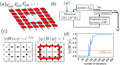
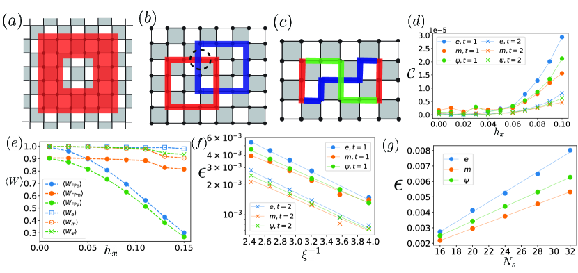
In this work, we propose a numerical method to systematically search for a complete set of Wilson loop operators for the case of Abelian topological orders, using only the ground state of a gapped Hamiltonian defined on a disk-like region of space. We do this by considering a variational ansatz for Wilson loop operators in terms of a matrix product operator with support on a ribbon along , as schematically shown in Fig. 1(a). We then set up a cost function in terms of the variational parameters of the WLOs. The minima of the cost function, which we numerically optimize for, gives the WLOs as diagrammatically shown in Fig. 1(c). The obtained Wilson loop operator expectation value can reach close to unity after a few hundred iterations (Fig. 1(d)). We emphasize that our procedure is unbiased and assumes no prior knowledge of the form of the WLOs.
Once the WLOs are obtained, we show how one can perform further optimization-based schemes to find operators that can create, move, and annihilate the anyons. Finally, we show that these operators can be utilized to extract the modular and matrices of an Abelian topological order, which gives a complete characterization of the topological order. In particular the and matrices encode all of the information about the fractional statistics.
We successfully demonstrate our numerical protocol in models with non-zero correlation lengths. For example, we show how one can extract the modular and matrices from only the ground states of the perturbed toric code and doubled semion models, with a Zeeman field that is up to half of the critical value.
To date, several invariants of two-dimensional topologically ordered states have been shown to be obtainable from the ground state wave function through a variety of methods. This includes the total quantum dimension measured through topological entanglement entropy kitaev2006topological ; levin2006detecting , the many-body Chern number and Hall conductance dehghani2021extraction ; cian2021many ; fan2022extracting , various invariants of symmetry-protected topological (SPT) states Shiozaki2017 ; Shiozaki2018many ; elben2020many , and the chiral central charge tu2013 ; zaletel2013 ; li2008 ; kim2021modular ; kim2021chiral . The modular and matrices, which encode details of the fractional statistics of the quasiparticles, can, under certain conditions, be extracted from the full set of ground states on a torus zhang2012quasiparticle ; zhang2015 ; wen1990naberry or in the presence of twist defects zhu2020 , but not to date from a single ground state on a disk.
We note that Ref. bridgeman2016 ; wahl2020local also proposed to find WLOs through an optimization approach, by searching for WLOs that commute with the Hamiltonian. However generic systems are not expected to have WLOs that commute with the Hamiltonian; instead as discussed above WLOs only appear as emergent symmetries that keep the ground state subspace invariant. Our work, in contrast to Ref.bridgeman2016 ; wahl2020local , uses only the ground state without requiring knowledge of the Hamiltonian.
The paper is organized as follows. In Sec. II, we review the basic properties of Wilson line operators and the algebraic theory of anyon. In Sec. III, we provide the optimization scheme for probing closed Wilson loop operators. In Sec. IV, we propose the scheme to create, move, annihilate anyons and measure the topological twist. We present numerical simulations for abelian topological order models in Sec. V. Finally, we provide an outlook for future works in Sec. VI.
II Wilson loop operators and anyon data
In this section, we briefly review the basic properties of WLOs and the algebraic theory of anyons. Since our goal is to extract topological invariants from the bulk of the wave function, in this section we consider a two dimensional system on an infinite plane.
The anyon theory consists of a collection of algebraic data that characterize the universal topological properties, namely the fusion and braiding properties, of the anyonic excitations of a many-body system. The precise mathematical framework is that of a unitary modular tensor category (UMTC). For reviews of UMTCs in the context of topological phases of matter, see for example Ref. kitaev2006 ; Bonderson07b ; wang2008 ; barkeshli2019 ; kawagoe2020microscopic . For a detailed discussion of how to relate the algebraic data of the UMTC to the microscopic properties of a quantum many-body system, see Ref. kawagoe2020microscopic .
The description that we provide below can be made exact in the context of exactly solvable models, such as the toric code and its generalizations, the quantum double and Levin-Wen models kitaev2003 ; levin2005string . The effect of perturbations to these exactly solvable models can also be studied systematically, using quasi-adiabatic continuation hastings2005quasiadiabatic . For chiral topological phases, such as fractional quantum Hall states or fractional Chern insulators, which have no description in terms of an exactly solvable model, it is expected that the same discussion applies, although it has not been explicitly studied outside of the context of field theory.
II.1 Anyons, Wilson line and loop operators
Since the system has a finite correlation length, we can define states with quasiparticle excitations that are localized on the scale of the correlation length. We can then group the quasiparticles into topological equivalence classes: two quasi-particle excitations are equivalent if and only if there is a local operator that can convert one into the other. The different equivalence classes define a finite set of distinct anyon types, sometimes also referred to as superselection sectors or topological charges, . The set of anyons contains the identity sector , which corresponds to excitations that can be created by local operators.
Since the anyonic excitations can be localized to within a correlation length of a particular point in space, we can consider a state with anyon type at position , and denote it as . In defining , we assume that far away from , on the scale of the correlation length , locally looks like the ground state. Furthermore, we assume any other non-trivial topological charges are infinitely far away and do not include them in labeling the state . Note that since refers to an equivalence class of excitations, there are many states that can be labeled as , so our choice is not unique.
By construction, the expectation value of any local observable satisfies , as long as and are far away from each other, , where is the ground state of the system and is the correlation length. The above equality holds up to corrections. Physically, this corresponds to the fact that the state has short-range correlations, so that a disturbance in the vicinity of has exponentially decreasing effects in the ground state beyond a correlation length.

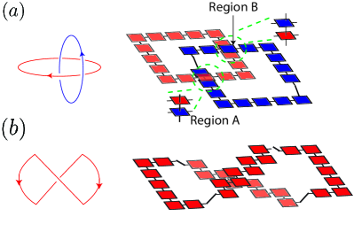
The anyons can be moved from one place to another by applying an operator along an arbitrary path. In particular, we define a Wilson line operator along a path starting at and ending at . moves the anyon excitation from position to along the path as shown in Fig. 2(a). Such operators are referred to as “movement operators” in kawagoe2020microscopic . Specifically,
| (1) |
In general, has support, up to exponentially small corrections, on a ribbon of thickness on the scale of , centered on . 222Specifically, can be approximated by a ribbon operator with finite thickness hastings2005quasiadiabatic . The error of the approximate Wilson line operator is of order , where is the number of sites in the support of , and is the exact, and presumably non-local WLO, for the ground state wave function . The precise choice of the operator is not unique in general, and a precise definition is also non-universal and depends on the microscopic details of the system. Nevertheless, encodes certain universal topological data that we wish to extract.
Note that in general need not be a unitary or even invertible operator, although in many simple examples, particularly when is an Abelian anyon, can be chosen to be unitary. Moreover, when is Abelian, we can take
| (2) |
where refers to the path traversed in the opposite direction and is the anti-particle of . That is, effectively takes along or, equivalently, takes along the path .
We can also define loop operators by picking in to be a closed loop. Physically this can be understood as creating and its dual out of the ground state, moving one around the loop , and reannihilating. If is a contractible loop in the space, such operators should keep the ground state invariant. Therefore, for each loop we have a loop operator , which keeps the ground state invariant:
| (3) |
Here is referred to as the quantum dimension of the anyon , and is part of the universal data of the UMTC. We have chosen a convention where appears on the RHS; we could in principle absorb into the definition of . The choice above allows us to make contact with the fusion algebra of the UMTC description.
As with the line operators, the Wilson loop operators are in general not unitary operators, unless is an Abelian anyon, in which case we also have .
Eq. 3 makes explicit that the ground state of a topologically ordered state has emergent symmetries, as there are loop operators that keep the ground state invariant. Importantly, the operators are supported, up to exponentially small corrections, on a codimension-1 region, and therefore do not correspond to ordinary global symmetries, which have support over the entire space. When the anyons are Abelian, the Wilson loop operators form a group structure and are referred to as 1-form symmetries gaiotto2014 ; more generally they are referred to as categorical or non-invertible symmetries.
II.2 Fusion rules and splitting operators
The anyons define a fusion algebra
| (4) |
where the fusion multiplicities are non-negative integers, which indicate the number of different ways the anyons and can be fused to produce the anyon type . Each anyon type has a unique anti-particle , where is such that . Note that we can define a fusion matrix , with entries ; the quantum dimension is then the largest eigenvalue of .
An anyon is Abelian if and only if it gives a unique fusion outcome upon fusing with another anyon . That is, given , for a unique and otherwise.
The fusion rule leads to the following relation for the Wilson loop operator:
| (5) |
whenever is a loop. Note that with the conventions chosen above, this implies .
In addition to movement operators and loop operators, we can define splitting operators. For simplicity, here we only introduce the spliting operator in the case ; the generalization can be found in Ref. kawagoe2020microscopic . Suppose that is contained in the fusion outcome of and , that is, . We can define a splitting operator,
| (6) |
where denotes a state with two excitations: anyon at position and anyon at position and as shown in Fig. 2(b).
One can also create the anyon and its antiparticle by applying
| (7) |
where is a state in the identity superselection sector.
Observe that if we start with a loop operator , and we project part of the operator along some segment of to the identity, then we obtain a cut operator that effective creates an anyon and its anti-particle out of the vacuum. Therefore we can obtain a choice of by starting with for a loop and implementing the above cutting procedure.
II.3 Modular matrix and twist product
A large portion of the universal data of a topological phase of matter is encoded in the modular and matrices. In fact for almost all topological phases of interest in physics, the and matrices provide a complete set of invariants.
The modular matrix contains information about the mutual braiding statistics between far separated anyon excitations, and also completely defines the fusion coefficients .
In particular, is the quantum mechanical amplitude of the process where a particle of type and another particle of type are created and separated, the particle is moved around the particle , and then the particle-anti-particle pairs are annihilated.
Given a set of closed Wilson loop operators , where , we can define a matrix , as
| (8) |
where is the twist product (see e.g. Ref. haah2016invariant ) and shown in Fig. 3. For arbitrary WLOs and defined in regions and as shown in Fig. 3(a), , , the twist product is defined as
| (9) |
where the product order is reversed in the region .
Note that to define the above twist product, we need each operator to have support strictly on a ribbon of finite thickness.
We expect that is related to as
| (10) |
where is the total quantum dimension. In this paper we only work with Abelian anyons, in which case and is the total number of distinct anyon types.
For Abelian anyons, the braiding phase between anyon and can be measured from the phase of the twist product
| (11) |
II.4 Modular matrix
The modular -matrix is a diagonal matrix,
| (12) |
where is the topological twist of the anyon . Due to the spin-statistics theorem, also corresponds to the exchange statistics of . In order to exchange a pair of identical anyons, we first create two anyon and anti-anyon pairs from the ground state, and we then move the two identical anyons and exchange them. Finally we fuse the anyon and anti-anyon and return the the ground state as shown in Fig. 3(b). If we normalize the process properly, the net effect of this procedure gives the exchange statistics of the anyons.
One can create and exchange anyons and measure the exchange statistics using the Wilson loop operators. The detailed implementation of the extraction of exchange statistics using the Wilson loop operators is given in Sec. IV.5.
III Optimization Scheme
In order to study the WLOs in the bulk of a ground state wave function, we propose a numerical scheme to extract contractible closed WLOs as defined in Eq. (3). We parametrize the WLOs by an ansatz based on matrix product operators (MPOs) verstraete2008matrix ; bridgeman2016 ; bultinck2017anyons . The ansatz is defined by two parameters: , where is a set of sites corresponding to the support of the WLO and is the bond dimension, as shown in Fig. 1. For a certain class of analytically solvable topologically ordered states, e.g. the Levin-Wen model and the Kitaev quantum double model, it is known that the WLOs can be efficiently expressed by MPOs with a support region with small thickness and bond dimension kitaev2003 ; levin2005string ; bultinck2017anyons .
To extract the closed WLOs using the MPO ansatz, we numerically optimize the MPO ansatz in order to obtain a which approximately satisfies Eq. (3). In order to efficiently optimize a Wilson loop, we note that for Abelian topological orders, an operator and a wave function satisfies Eq. (3) if and only if
| (13) | |||
| (14) |
The forward proof is trivial. For the backward proof, we assume that and satisfy Eqs. (13) and (14) and without loss of generality, , where and are complex numbers and . Solving Eqs. (13) and (14) we can obtain and . Note that Eq. (11) implies that and Eq. (12) ensures that is normalized to , which then requires .
Therefore, we can define the cost function for a wave function as
| (15) |
It reaches a global minimum only when is an exact Wilson loop operator.
To variationally optimize the WLO, we start by initializing a random MPO with fixed . Each tensor in the MPO is initialized randomly and independently from each other. For a translationally invariant system, one may naively expect that a translation symmetric closed WLO is a better ansatz. However, we found that the translation symmetric ansatz tends to be unstable numerically, leading to diverging or vanishing gradients in the optimization procedure.
After the initialization, we minimize the cost function defined in Eq. (15) through gradient based optimization. In this work, we apply the Adam algorithm kingma2014adam to minimize the cost function. In this work, we fix the hypermeters of the Adam algorithm as and learning rate . We iterate the optimization procedure until the cost function converges, which typically takes a few hundred to a few thousand iterations.
We repeat the initialization and minimization times to obtain optimized WLOs , where . Throughout the manuscript, we fix . We then measure the braiding phases and topological twists to classify the WLOs through the equivalence relation described as follows : we compute the mutual-braiding phases between and , , where and topological twist for , where . We say the two WLOs and are equivalent when for , and . After grouping the WLOs into equivalence classes, we randomly pick one representative WLO from each equivalent class.
This equivalence relation assumes that if two WLOs have the same braiding phase with the rest of the WLOs and identical topological twists, the two WLOs are equivalent. We note that this condition only holds when we obtain a complete set of WLOs in our optimization procedure. Missing one could result in a false classification. However, one can verify whether a complete set of WLOs is found by checking if the resulting matrix is a unitary matrix. If one or more WLOs are missing, we can vary the hyper-parameters such as increasing the thickness of the WLOs or the bond dimension .
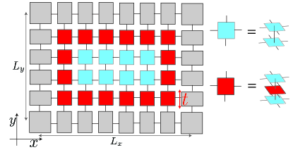
The bottleneck of the numerical optimization is in the tensor contraction when calculating the expectation values and . Here, we briefly describe the tensor contraction scheme and its computational time complexity. Given a ground state wave function , represented by an infinite projective entangled pair state (iPEPS) orus2009simulation ; liao2019differentiable ; crone2020detecting as shown in Fig. 4 , we use the following procedure to evaluate the expectation value . Consider a closed WLO that takes the form of a rectangular loop with side lengths and as shown in Fig. 4, for a system on a square lattice. We first contract all tensors at to form a tensor with bonds as shown in Fig. 4. We then contract the tensors at with one by one from to . We then repeat this procedure for all . In this contraction procedure, the computational cost for contracting the tensors scales linearly with the number of sites along the direction () and exponentially with number of sites along the direction (). Therefore, the total computational cost is bounded by . Moreover, since the thickness and the size of the hole need to be much larger than the correlation length, we have that . Thus the total computational cost for calculating the expectation value scales up as for some constant . Therefore, this method is particularly suitable for models with small correlation length. Importantly, the complexity of the computation scales with the correlation length, not the total system size.
IV Manipulation of anyons
Once we have obtained the closed WLOs, we can extract many non-trivial properties of the anyons. In particular, we can further obtain operators that create, move, and annihilate anyons.
In the following, we discuss how to manipulate anyons by starting from the closed WLOs. For simplicity in this section, we assume that the thickness of WLOs is . The idea can be easily generalized to as is the case for our numerical results in Section V.
IV.1 Removing and adding a virtual bond
Before we proceed to the manipulation of anyons, we first define two basic operations of a tensor , which is that of removing and adding a virtual bond. These two operations will be extensively used throughout this section.
Removing a virtual bond is useful for cutting open closed WLOs. To remove a virtual bond in a tensor , we define an edge tensor that describes the boundary condition and contract the edge tensor with ; the resulting tensor is
| (16) |
and it has rank .
Adding a virtual bond is useful when extending an open WLO or connecting two open WLOs. To add a trivial virtual bond to an arbitrary tensor with rank , we define a new tensor with rank as
| (17) |
for all , where is the bond dimension of the new virtual bond.
Using the above two basic operations on tensors, we can create, move and annihilate anyons, as described in the following sections.
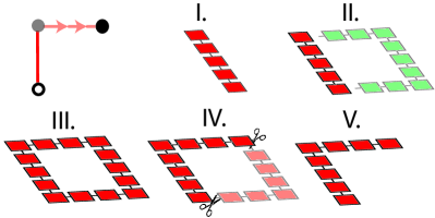
IV.2 Creation of anyon and anti-anyon pairs
To create an anyon and anti-anyon pair, we simply discard a segment of the closed WLO and apply an arbitrary edge tensor to terminate its boundary as shown in Fig. 5. Specifically, we start with a closed WLO obtained using the procedure described in Sec. III for a give ground state wave function , which is of the form
| (18) |
where is the length of the closed WLO.
We then keep the tensors from sites , as shown in step I of Fig. 5, so that the new MPO is of the form
| (19) |
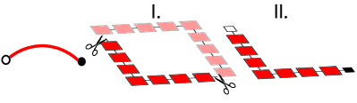
We then remove the virtual indices and by applying the edge tensor . The edge tensors can be chosen arbitrarily, since different choices are related to each other by a local operator. Throughout out this article, we use
| (20) |
After removing the edge virtual bond shown in step II in Fig. 5, the open WLO is of the form
| (21) |
When another WLO passes through the open WLO, the system acquires an anyonic braiding phase as long as the crossing point is away from the boundary of the open WLO by an .
Finally, in order to preserve the norm of the wave function, we normalize the open WLO defined above by a factor .
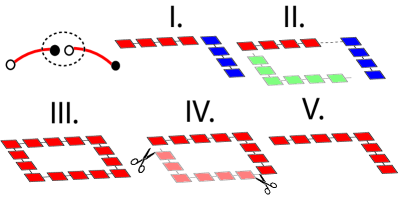
IV.3 Moving anyons
Let us imagine we have a WLO that creates an anyon at one endpoint and its conjugate at the other endpoint . We can use this to construct a different operator , effectively moving from to . We can do this as follows.
We start with an open WLO as shown in step I of Fig. 6. The open WLO with length is of the form
| (22) |
The open WLO can be obtained using the procedure described in Sec. IV.2.
We initialize another random MPO with length that is a loop complement of the WLO as shown in step II of Fig. 6 and is of the form
| (23) |
To connect and at the boundary, we add a trivial virtual bond on each boundary tensor. By adding trivial virtual bond on all the boundary tensors , we have
We can therefore have a closed WLO of the form
| (25) |
where is a Kronecker delta function.
In step III of Fig. 6, we minimize the cost function of Eq. (15) for the closed WLO defined above. We note that in addition to vary the tensors in the , we also have to vary tensors at the boundary of i.e. , ,…etc. in order to eliminate the anyon excitation at the boundary.
We define a length parameter , which is of order . In the optimization procedure, we vary all the tensors s and s in and the boundary tensor of , , , , and , , , while fixing the tensors for .
IV.4 Annihilation of anyon and anti-anyon pairs
In this section, we describe a procedure to fuse an anyon and anti-anyon pair to identity. Given two open WLOs and , we show how to join them into a single WLO, as shown in Fig. 7, by effectively bringing together two endpoints of and and annihilating the anyons.
We consider two open WLOs of the form
| (26) |
For simplicity we assume that the tensors and are located at nearest-neighbor sites as shown in step I of Fig. 6. If this is not the case, we can move the end of using the procedure described in Sec. IV.3.
We then initialize a random MPO with length that is a loop complement of and , which takes the form
| (27) |
We can connect the three open WLOs by adding a trivial virtual bond on each boundary tensor as in step III of Fig. 7. After adding a virtual bond, the WLOs become
| (28) |
We can therefore connect the three WLO and have a closed MPO of the form
| (29) |
IV.5 Topological twist (exchange statistics)
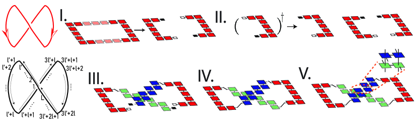
Here we present the scheme that we use to extract the topological twists of the anyons. To calculate the topological twists, we calculate the ratio of the amplitude for the following two processes. In the first process (), we create an anyon and anti-anyon pair from the ground state wave function. We then exchange them, and finally, we annihilate the pair of anyon and anti-anyon. In the second process (), we create and annihilate the pair directly without any exchange
For the first process, we start with a closed WLO with length of the form
| (30) |
We then cut the closed WLO and keep two segments with length as shown in step I of Fig. 8. These segments represent a creation of an anyon and anti-anyon. The end of the two segments of the WLOs are away from each other by distance which is an integer larger than .
The WLOs are of the form
In Step II, we flip the direction of the anyon transport for the WLO by applying Hermitian conjugation.
After cutting and flipping the WLO, we move the anyon located at the open ends and to sites and respectively, as shown in step III of Fig. 8. We then connect the WLOs by annihilating anyon and anti-anyon pairs in step IV of Fig. 8. The WLO becomes a self-intersecting closed loop of the form
| (32) |
where is the path length of the closed WLO . The labels for the supports are shown in Fig. 8. Finally, we contract the physical indices in the self-intersecting region as shown in step V of Fig. 8.
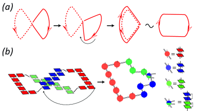
In step I of process , we cut and discard two segments of a closed WLO as described in Eq. (LABEL:eq_twist_two_segs). This step explicitly breaks the gauge symmetry of a matrix product operator, which introduces non-universal complex phases to and . The non-universal complex phase depends on the details of the implementation. In order to cancel the non-universal complex phase, we calculate the amplitude of the second process using the same tensors in Eq. (32), but we contract the tensors without exchanging anyons. We conjecture and numerically verify that the process has the same non-universal complex phase as the process . The calculation of process can be achieved by rotating the right half of the support of around the center of self-intersecting region and stacking it on top of the left half of the support as shown in Fig. 9(a). Instead of creating, exchanging and annihilating the anyon and anti-anyon pair, this process creates an anyon and anti-anyon pair and the anyon travels around the left half of the support twice. And subsequently it is annihilated with the anti-anyon. We note that in order to perform the rotation, presumably the ground state wave function must have rotation symmetry around the center of the self-intersecting region and translation symmetry. We have not systematically studied how the above procedure would need to be modified if the translation and rotation symmetries of the system are broken.
The WLO after the rotation is of the following form
where
| (34) |
and the tensor multiplication denotes the contraction of physical indices as shown in Fig. 9(b).
Therefore, the topological twist that represents the exchange statistics is calculated from the ratio of the expectation value of and ,
| (35) |
where the label denotes the anyon type.
V Numerical results
In this section, we present the numerical results for extracting WLOs and braiding statistics for various systems.
V.1 toric code model in a magnetic field
We first consider the toric code model in a magnetic (Zeeman) field wu2012phase ; vidal2009low ; tupitsyn2010topological ; halasz2012probing ; ritz2021wegner . The Hamiltonian is of the form
| (36) |
where the plaquette operators , the vertex operators and and are the magnetic fields along the and directions respectively.
In the following, we consider a dual lattice, so that the spins are on the lattice sites instead of the bonds. The plaquette operators and the vertice operators of the toric code model are then on alternating plaquettes, as depicted in gray and white respectively in Fig. 10 (a).
When the magnetic fields , the ground state of the toric code model can be solved analytically. The ground state has zero correlation length and the Wilson loop operators can be solved exactly (cost ) with bond dimension and thickness for any size of the closed WLOs and .
There exist four distinct Wilson loop operators for the anyon types : , , and , where is the identity sector, and are bosons with trivial self-braiding phase and a mutual-braiding phase and is the fermion. The modular matrix characterizing the mutual braiding statistics, listing the anyons in the order , , , is of the form,
| (37) |
The topological twists, which characterize the exchange statistics of the anyons, is given by
| (38) |
Figure 10 (b) and (c) illustrate the measurement of modular and matrices with thickness on 2D square lattice.
With non-zero magnetic fields, the ground state wave function has a finite correlation length . The Wilson loop operators with finite thickness can no longer represent the exact WLOs. However, the optimization scheme can still find approximate WLOs with error of order , where is the number of sites.
We first obtain the ground state wave function by minimizing the infinite projective entangled pair state (iPEPS) using a recently proposed differential programming approach liao2019differentiable ; crone2020detecting with corner transfer matrix renormalization group (CTMRG) orus2009simulation .
Next, we follow the protocol described in Sec. III, minimizing the cost function defined in Eq. (15) starting from random MPO initializations, to find the Wilson loop operators. Figure 10(d) shows the minimum cost as a function of with a fixed for thickness and . The cost decreases when the thickess increases, demonstrating that a larger thickness gives a better approximation to the true Wilson loop operator.
In Fig. 10(e), we compare the optimized closed WLOs to the WLOs known for the fixed point toric code Hamiltonian (). The expectation values of the optimized closed WLOs stay close to as the magnetic field is increased. However, the expectation values of the fixed point WLOs decrease with increasing . We note that this is remarkable given that we do not use prior knowldge of the WLOs of the fixed point Hamiltonian; our scheme is completely unbiased and uses no prior information aside from the ground state of the perturbed Hamiltonian whose WLOs we are trying to find.
While we do not know the form of the exact WLOs in the presence of non-zero , , we do know that their expectation value in the ground state is 1. Therefore, we can compute how close our optimized WLOs are to the exact WLOs. We define the error
| (39) |
where we use the fact that the exact WLO, , satisfies . Here represents a WLO found through our optimization protocol.
We present the error of the WLOs as a function of the inverse of the correlation length and number of sites in Fig. 10(f) and (g), respectively The correlation length is computed by through the exponential decay of the correlation funcion, . The largest correlation length we reach in our simulation is .
In Fig. 10(f), we vary the correlation length by varying the magnetic field . We show that the error drops exponentially as function of . Fig. 10 (g) shows how the error scales with the number of sites in the support of the WLO with , indicating that the error scales up linearly with . Therefore the error scaling is consistent with the error bound hastings2005quasiadiabatic .
Finally, we numerically evaluate the twist product matrix and the topological twist . The twist product matrix is consistent with Eq. (37) up to error and the topological twist has error up to . For example, the twist product matrix for , , , , , is
| (40) |
and
| (41) |
V.2 Double semion model
In this section, we present our numerical results for the double semion model.
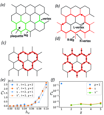
The Hamiltonian of the double semion model levin2005string , which we take to be on the honeycomb lattice, is of the form
| (42) | |||||
where the plaquette operators , the vertex operators and legs is the legs of plaquette as shown in Fig. 11(a).
For , the ground state and the Wilson loop operators can be obtained analytically levin2005string . There exists four distinct WLOs denoted by , , , , which represent identity, right and left-handed semions and a boson. The two semions have self-braiding statistics and trivial mutual braiding statistics. The modular matrix, listing the anyons in the order , , , , is of the form
| (43) |
The topological twists that characterize the exchnage statistics of the double semion model is given by
| (44) |
The exact closed WLOs for are of the form
| (45) |
where is a path of a closed WLO, is a path of a closed WLO on the duel lattice, and are two legs attached to L-vertex as shown in Fig. 11(b).
Note that the and operators above have thickness and bond dimension . Interestingly, using our unbiased numerical optimization, we found an equivalent way to represent the exact WLOs at the fixed point with and . We present its analytical form in Appendix A.
In order to numerically optimize the WLOs, we numerically optimize the iPEPS ground state wave function corboz2012simplex and consider WLOs with thickness and as shown in Fig. 11(c) and 11(d) respectively. Fig. 11(e) shows the minimum cost achieved as a function of the magnetic field . The optimizer converges to these minimum costs after roughly 1000 iterations. Fig. 11(f) shows the minimum cost as a function of the bond dimension for the two semions for and .
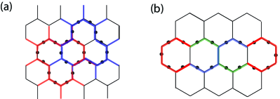
We then numerically evaluate the twist product matrix and the topological twist . The support of and are shown in Fig. 12(a) and (b) respectively. The twist product matrix is consistent with Eq. (43) up to error and the topological twist has error up to . For example, the twist product matrix for , , is
| (46) |
and
| (47) |
The correlation length of the ground state, calculated through the exponential decay of the correlation funcion, , with is .
VI Summary and outlook
In conclusion, we propose a numerical optimization-based scheme to extract Wilson loop operators of anyons from a single ground state wave function defined on a simply connected region of space. We show how, after extracting closed loop operators, one can then modify them to obtain Wilson line operators that create, move, and annihilate anyons. This allows us to ultimately extract the braiding statistics and topological twists of the anyons from a single bulk ground state wave function. While our protocol for extracting the modular matrix is expected to be general, our protocol for extracting the topological twists may be benefiting from the lattice symmetries of our models; we leave a systematic investigation of this for future work.
Our algorithm fully succeeds only when all distinct equivalence classes of Wilson loop operators have been found. We expect that in general, for a large enough bond dimension, all Wilson loop operators can be captured by our matrix product operator ansatz. In practice it may be the case that some Wilson loop operators might be more complicated than others, in the sense of having higher operator entanglement or requiring larger bond dimension. In this case, if there is an implicit bias of the optimization procedure towards the simpler loop operators, then the algorithm may never succeed in discovering a complete set of loop operators starting from random initialization. In this case, further work needs to be done on either finding improved initializations or modifying the optimization procedure to remove the implicit biases.
Our work also raises an interesting question of whether all Wilson loop operators for anyons can always be described by an MPO with finite bond dimension. This is particularly intriguing to study for chiral topological orders, such as fractional quantum Hall states, where loop operators have never been explicitly computed in MPO form and the ground state wave functions cannot be described by a PEPS with finite bond dimension.
So far, our optimization scheme is tailored to Abelian topological orders. It would be interesting to generalize it to the case of non-abelian topologically ordered phases, which can have anyons with quantum dimension greater than one. One possible direction is to design an optimization scheme to extract both the WLOs and the quantum dimension of anyons simultaneously.
As we discussed, the Wilson line operators can be generalized to more generic movement and splitting operators. If we discover such generic movement and splitting operators through a similar optimization approach to what we have described, it may also be possible to extract the and symbols of the underlying modular tensor category using the results of Ref. kawagoe2020microscopic .
Looking further, similar optimization procedures applied to symmetry defect creation and movement operators may eventually allow us to extract the full -crossed braided tensor category barkeshli2019 that describes a given symmetry-enriched topological ground state. This would allow the extraction of all possible topological invariants from a single bulk ground state wave function.
More broadly, recent developments in quantum simulators allow the realization of topologically ordered states that might not occur in conventional electronic matter Googletoric2021 ; HarvardQSL1 . Given this opportunity, it is intriguing to develop measurement protocols for probing topological properties of a ground state wave function associated with a prior unknown gapped Hamiltonian. Our optimization protocol may be particularly relevant in this context. Since our scheme requires measuring several observables for a given wave function, it may be useful when combined with shadow tomography. huang2020predicting .
VII Acknowledgements
This work is supported by NSF CAREER DMR- 1753240 (MB), AFOSR-MURI FA9550- 19-1-0399, ARO W911NF2010232, ONR N00014-20-1-2325, National Science Foundation QLCI grant OMA-2120757, U.S. Department of Energy, Quantum Systems Accelerator program and the Simons and Minta Martin Foundations (MH,ZC).
Appendix A Alternative definition of Wilson loop operator for double semion model
In Eq. (45), the operators applied on the R-leg are . The operator in the exponent is equivalent to in the space spanned by close string configurations as shown in fig. 13(a), where and are the two sites attached to the same vertex of the R-leg . Therefore, the Wilson loop operators can be rewritten as
where is a path of a closed WLO, denotes R-vertex and and are two legs attached to R-vertex as shown in fig. 11(b).

To show that the WLOs in Eq. (LABEL:Wilson_DS_alternative) can be represented by MPOs with , , we consider an open Wilson operator shown in fig. 13(b) which creates semions on the both ends of the Wilson operator for illustration. A closed WLO can be defined in a similar fashion. To simplify the notation, we define for right and left-handed semion respectively and . The Wilson loop operators can be represented in the tensor network notation as shown in 13(b). The operators and can be decomposed through singular value decomposition (SVD) as
| (49) |
where is the index auxiliary bond as shown in fig. 13(c) and
| (50) |
where . After SVD, the Wilson operators can be expressed by a two-site periodic MPO terminated by edge tensors :
where , , and . can be defined similarly. Therefore, the WLO for creating semions can be expressed by MPO with and .
References
- [1] Xiao-Gang Wen. Quantum Field Theory of Many-Body Systems. Oxford Univ. Press, Oxford, 2004.
- [2] Chetan Nayak, Steven H. Simon, Ady Stern, Michael Freedman, and Sankar Das Sarma. Non-abelian anyons and topological quantum computation. Rev. Mod. Phys., 80:1083, 2008.
- [3] Zhenghan Wang. Topological Quantum Computation. American Mathematical Society, 2008.
- [4] T. Senthil. Symmetry-protected topological phases of quantum matter. Annual Review of Condensed Matter Physics, 6:299–324, 2015.
- [5] Bei Zeng, Xie Chen, Duan-Lu Zhou, Xiao-Gang Wen, et al. Quantum information meets quantum matter. Springer, 2019.
- [6] Maissam Barkeshli, Parsa Bonderson, Meng Cheng, and Zhenghan Wang. Symmetry fractionalization, defects, and gauging of topological phases. Phys. Rev. B, 100:115147, Sep 2019.
- [7] Kyle Kawagoe and Michael Levin. Microscopic definitions of anyon data. Physical Review B, 101(11):115113, 2020.
- [8] Daniel Bulmash and Maissam Barkeshli. Fermionic symmetry fractionalization in 2+1 dimensions. Physical Review B, 105(12), mar 2022.
- [9] David Aasen, Parsa Bonderson, and Christina Knapp. Characterization and classification of fermionic symmetry enriched topological phases. arXiv preprint arXiv:2109.10911, 2021.
- [10] K. J. Satzinger et al. Realizing topologically ordered states on a quantum processor. Science, 374(6572):1237–1241, 2021.
- [11] G. Semeghini, H. Levine, A. Keesling, S. Ebadi, T. T. Wang, D. Bluvstein, R. Verresen, H. Pichler, M. Kalinowski, R. Samajdar, A. Omran, S. Sachdev, A. Vishwanath, M. Greiner, V. Vuletic, and M. D. Lukin. Probing topological spin liquids on a programmable quantum simulator. Science, 374(6572):1242–1247, 2021.
- [12] Dolev Bluvstein, Harry Levine, Giulia Semeghini, Tout T Wang, Sepehr Ebadi, Marcin Kalinowski, Alexander Keesling, Nishad Maskara, Hannes Pichler, Markus Greiner, et al. A quantum processor based on coherent transport of entangled atom arrays. arXiv preprint arXiv:2112.03923, 2021.
- [13] Matthew B Hastings and Xiao-Gang Wen. Quasiadiabatic continuation of quantum states: The stability of topological ground-state degeneracy and emergent gauge invariance. Physical review b, 72(4):045141, 2005.
- [14] Davide Gaiotto, Anton Kapustin, Nathan Seiberg, and Brian Willett. Generalized global symmetries. 2014.
- [15] A.Yu. Kitaev. Fault-tolerant quantum computation by anyons. Annals Phys., 303:2–30, 2003.
- [16] Michael A Levin and Xiao-Gang Wen. String-net condensation: A physical mechanism for topological phases. Physical Review B, 71(4):045110, 2005.
- [17] Alexei Kitaev and John Preskill. Topological entanglement entropy. Physical review letters, 96(11):110404, 2006.
- [18] Michael Levin and Xiao-Gang Wen. Detecting topological order in a ground state wave function. Physical review letters, 96(11):110405, 2006.
- [19] Hossein Dehghani, Ze-Pei Cian, Mohammad Hafezi, and Maissam Barkeshli. Extraction of the many-body chern number from a single wave function. Physical Review B, 103(7):075102, 2021.
- [20] Ze-Pei Cian, Hossein Dehghani, Andreas Elben, Benoît Vermersch, Guanyu Zhu, Maissam Barkeshli, Peter Zoller, and Mohammad Hafezi. Many-body chern number from statistical correlations of randomized measurements. Physical Review Letters, 126(5):050501, 2021.
- [21] Ruihua Fan, Rahul Sahay, and Ashvin Vishwanath. Extracting the quantum hall conductance from a single bulk wavefunction. arXiv preprint arXiv:2208.11710, 2022.
- [22] Ken Shiozaki and Shinsei Ryu. Matrix product states and equivariant topological field theories for bosonic symmetry-protected topological phases in (1+1) dimensions. Journal of High Energy Physics, 2017(4):100, Apr 2017.
- [23] Ken Shiozaki, Hassan Shapourian, Kiyonori Gomi, and Shinsei Ryu. Many-body topological invariants for fermionic short-range entangled topological phases protected by antiunitary symmetries. Phys. Rev. B, 98:035151, Jul 2018.
- [24] Andreas Elben, Jinlong Yu, Guanyu Zhu, Mohammad Hafezi, Frank Pollmann, Peter Zoller, and Benoît Vermersch. Many-body topological invariants from randomized measurements in synthetic quantum matter. Science advances, 6(15):eaaz3666, 2020.
- [25] Hong-Hao Tu, Yi Zhang, and Xiao-Liang Qi. Momentum polarization: An entanglement measure of topological spin and chiral central charge. Physical Review B, 88(19), Nov 2013.
- [26] Michael P. Zaletel, Roger S. K. Mong, and Frank Pollmann. Topological characterization of fractional quantum hall ground states from microscopic hamiltonians. Physical Review Letters, 110(23), Jun 2013.
- [27] Hui Li and F. D. M. Haldane. Entanglement spectrum as a generalization of entanglement entropy: Identification of topological order in non-abelian fractional quantum hall effect states. Phys. Rev. Lett., 101:010504, Jul 2008.
- [28] Isaac H Kim, Bowen Shi, Kohtaro Kato, and Victor V Albert. Modular commutator in gapped quantum many-body systems. arXiv preprint arXiv:2110.10400, 2021.
- [29] Isaac H Kim, Bowen Shi, Kohtaro Kato, and Victor V Albert. Chiral central charge from a single bulk wave function. arXiv preprint arXiv:2110.06932, 2021.
- [30] Yi Zhang, Tarun Grover, Ari Turner, Masaki Oshikawa, and Ashvin Vishwanath. Quasiparticle statistics and braiding from ground-state entanglement. Physical Review B, 85(23):235151, 2012.
- [31] Yi Zhang, Tarun Grover, and Ashvin Vishwanath. General procedure for determining braiding and statistics of anyons using entanglement interferometry. Physical Review B, 91(3), Jan 2015.
- [32] X.G. Wen. Topological orders in rigid states. Int. J. Mod. Phys., B:239, 1990.
- [33] Guanyu Zhu, Mohammad Hafezi, and Maissam Barkeshli. Quantum origami: Transversal gates for quantum computation and measurement of topological order. Physical Review Research, 2(1), Mar 2020.
- [34] Jacob C. Bridgeman, Steven T. Flammia, and David Poulin. Detecting topological order with ribbon operators. Physical Review B, 94(20), Nov 2016.
- [35] Thorsten B Wahl and Benjamin Béri. Local integrals of motion for topologically ordered many-body localized systems. Physical Review Research, 2(3):033099, 2020.
- [36] Alexei Kitaev. Anyons in an exactly solved model and beyond. Ann. Phys., 321(1):2 – 111, 2006.
- [37] Parsa Hassan Bonderson. Non-Abelian Anyons and Interferometry. PhD thesis, California Institute of Technology, 2007.
- [38] Jeongwan Haah. An invariant of topologically ordered states under local unitary transformations. Communications in Mathematical Physics, 342(3):771–801, 2016.
- [39] Frank Verstraete, Valentin Murg, and J Ignacio Cirac. Matrix product states, projected entangled pair states, and variational renormalization group methods for quantum spin systems. Advances in physics, 57(2):143–224, 2008.
- [40] Nick Bultinck, Michael Mariën, Dominic J Williamson, Mehmet B Şahinoğlu, Jutho Haegeman, and Frank Verstraete. Anyons and matrix product operator algebras. Annals of physics, 378:183–233, 2017.
- [41] Diederik P Kingma and Jimmy Ba. Adam: A method for stochastic optimization. arXiv preprint arXiv:1412.6980, 2014.
- [42] Román Orús and Guifré Vidal. Simulation of two-dimensional quantum systems on an infinite lattice revisited: Corner transfer matrix for tensor contraction. Physical Review B, 80(9):094403, 2009.
- [43] Hai-Jun Liao, Jin-Guo Liu, Lei Wang, and Tao Xiang. Differentiable programming tensor networks. Physical Review X, 9(3):031041, 2019.
- [44] SPG Crone and P Corboz. Detecting a z 2 topologically ordered phase from unbiased infinite projected entangled-pair state simulations. Physical Review B, 101(11):115143, 2020.
- [45] Fengcheng Wu, Youjin Deng, and Nikolay Prokof’ev. Phase diagram of the toric code model in a parallel magnetic field. Physical Review B, 85(19):195104, 2012.
- [46] Julien Vidal, Sébastien Dusuel, and Kai Phillip Schmidt. Low-energy effective theory of the toric code model in a parallel magnetic field. Physical Review B, 79(3):033109, 2009.
- [47] IS Tupitsyn, Alexei Kitaev, NV Prokof Ev, and PCE Stamp. Topological multicritical point in the phase diagram of the toric code model and three-dimensional lattice gauge higgs model. Physical Review B, 82(8):085114, 2010.
- [48] Gábor B Halász and Alioscia Hamma. Probing topological order with rényi entropy. Physical Review A, 86(6):062330, 2012.
- [49] Anna Ritz-Zwilling, Jean-Noël Fuchs, and Julien Vidal. Wegner-wilson loops in string nets. Physical Review B, 103(7):075128, 2021.
- [50] Philippe Corboz, Karlo Penc, Frédéric Mila, and Andreas M Läuchli. Simplex solids in su (n) heisenberg models on the kagome and checkerboard lattices. Physical Review B, 86(4):041106, 2012.
- [51] Hsin-Yuan Huang, Richard Kueng, and John Preskill. Predicting many properties of a quantum system from very few measurements. Nature Physics, 16(10):1050–1057, 2020.