Conformal Prediction is Robust to Dispersive Label Noise

Abstract

We study the robustness of conformal prediction, a powerful tool for uncertainty quantification, to label noise. Our analysis tackles both regression and classification problems, characterizing when and how it is possible to construct uncertainty sets that correctly cover the unobserved noiseless ground truth labels. We further extend our theory and formulate the requirements for correctly controlling a general loss function, such as the false negative proportion, with noisy labels. Our theory and experiments suggest that conformal prediction and risk-controlling techniques with noisy labels attain conservative risk over the clean ground truth labels except in adversarial cases. In such cases, we can also correct for noise of bounded size in the conformal prediction algorithm in order to ensure achieving the correct risk of the ground truth labels without score or data regularity.

1 Introduction

In most supervised classification and regression tasks, one would assume the provided labels reflect the ground truth. In reality, this assumption is often violated; see (Cheng et al., 2022; Xu et al., 2019; Yuan et al., 2018; Lee and Barber, 2022; Cauchois et al., 2022). For example, doctors labeling the same medical image may have different subjective opinions about the diagnosis, leading to variability in the ground truth label itself. In other settings, such variability may arise due to sensor noise, data entry mistakes, the subjectivity of a human annotator, or many other sources. In other words, the labels we use to train machine learning (ML) models may often be noisy in the sense that these are not necessarily the ground truth. Quantifying the prediction uncertainty is crucial in high-stakes applications in general, and especially so in settings where the training data is inexact. We aim to investigate uncertainty quantification in this challenging noisy setting via conformal prediction, a framework that uses hold-out calibration data to construct prediction sets that are guaranteed to contain the ground truth labels; see (Vovk et al., 2005; Angelopoulos and Bates, 2021). Additionally, we analyze the effect of label noise on risk-controlling techniques, which extend the conformal approach to construct uncertainty sets with a guaranteed control over a general loss function (Bates et al., 2021; Angelopoulos et al., 2021, 2022). In short, this paper outlines the fundamental conditions under which conformal prediction and risk-controlling methods still work under label noise, and furthermore, studies its behavior with several common loss functions and noise models.

We adopt a variation of the standard conformal prediction setup. Consider a calibration data set of i.i.d. observations $\{(X_{i},Y_{i})\}_{i=1}^{n}$ sampled from an arbitrary unknown distribution $P_{XY}$. Here, $X_{i}\in\mathbb{R}^{p}$ is the feature vector that contains $p$ features for the $i$-th sample, and $Y_{i}$ denotes its response, which can be discrete for classification tasks or continuous for regression tasks. Given the calibration dataset, an i.i.d. test data point $(X_{\rm test},Y_{\rm test})$, and a pre-trained model $\hat{f}$, conformal prediction constructs a set $\widehat{\mathcal{C}}(X_{\rm test})$ that contains the unknown test response, $Y_{\rm test}$, with high probability, e.g., 90%. That is, for a user-specified level $\alpha\in(0,1)$,

$$\mathbb{P}\left(Y_{\rm test}\in\widehat{\mathcal{C}}(X_{\rm test})\right)\geq 1-\alpha.$$ (1)

This property is called marginal coverage, where the probability is defined over the calibration and test data.

In the setting of label noise, we only observe the corrupted labels $\tilde{Y}_{i}=g(Y_{i})$ for some corruption function $g:\mathcal{Y}\times[0,1]\to\mathcal{Y}$, so the i.i.d. assumption and marginal coverage guarantee are invalidated. The corruption is random; we will always take the second argument of $g$ to be a random seed $U$ uniformly distributed on $[0,1]$. To ease notation, we leave the second argument implicit henceforth. Nonetheless, using the noisy calibration data, we seek to form a prediction set $\widehat{\mathcal{C}}_{\rm noisy}(X_{\rm test})$ that covers the clean, uncorrupted test label, $Y_{\rm test}$. More precisely, our goal is to delineate when it is possible to provide guarantees of the form

$$\mathbb{P}\left(Y_{\rm test}\in\widehat{\mathcal{C}}_{\rm noisy}(X_{\rm test})\right)\geq 1-\alpha,$$ (2)

where the probability is taken jointly over the calibration data, test data, and corruption function (this will be the case for the remainder of the paper). Note that this goal is impossible in general—see Proposition 2.3. However, we present some realistic noise models under which (2) is satisfied. Furthermore, in our real-data experiments, conformal prediction and risk-controlling methods normally achieve conservative risk/coverage even with access only to noisy labels. There is a particular type of anti-dispersive noise that causes failure, and we see this both in theory and practice. If such noise can be avoided, a user should feel safe deploying uncertainty quantification techniques even with noisy labels.

1.1 Related work

Conformal prediction was first proposed by Vladimir Vovk and collaborators (Vovk et al., 1999, 2005). Recently, there has been a body of work studying the statistical properties of conformal prediction (Lei et al., 2018; Barber, 2020) and its performance under deviations from exchangeability (Tibshirani et al., 2019; Podkopaev and Ramdas, 2021; Barber et al., 2022). Label noise independently of conformal prediction has been well-studied; see, for example (Angluin and Laird, 1988; Tanno et al., 2019; Frénay and Verleysen, 2013). To our knowledge, conformal prediction under label noise has not been previously analyzed. The closest work to ours is that of Cauchois et al. (2022), studying conformal prediction with weak supervision, which could be interpreted as a type of noisy label.

2 Conformal Prediction

2.1 Background

As explained in the introduction, conformal prediction uses a held-out calibration data set and a pre-trained model $\hat{f}$ to construct the prediction set on a new data point. More formally, we use the model $\hat{f}$ to construct a score function, $s:\mathcal{X}\times\mathcal{Y}\to\mathbb{R}$, which is engineered to be large when the model is uncertain and small otherwise. We will introduce different score functions for both classification and regression as needed in the following subsections.

Abbreviate the scores on each calibration data point as $s_{i}=s(X_{i},Y_{i})$ for each $i=1,...,n$. Conformal prediction tells us that we can achieve a marginal coverage guarantee by picking $\hat{q}_{\rm clean}=s_{(\lceil(n+1)(1-\alpha)\rceil)}$ as the $\lceil(n+1)(1-\alpha)\rceil$-smallest of the calibration scores and constructing the prediction sets as

$$\widehat{\mathcal{C}}\left(X_{\rm test}\right)=\left\{y\in\mathcal{Y}:s\left(X_{\rm test},y\right)\leq\hat{q}_{\rm clean}\right\}.$$ (3)

In this paper, we do not allow ourselves access to the calibration labels, only their noisy versions, $\tilde{Y}_{1},\ldots,\tilde{Y}_{n}$, so we cannot calculate $\hat{q}_{\rm clean}$. Instead, we can calculate the noisy quantile $\hat{q}_{\rm noisy}$ as the $\lceil(n+1)(1-\alpha)\rceil$-smallest of the noisy score functions, $\tilde{s}_{i}=s(X_{i},\tilde{Y}_{i})$. The main formal question of our work is whether the resulting prediction set, $\widehat{\mathcal{C}}_{\rm noisy}(X_{\rm test})=\{y:s(X_{\rm test},y)\leq\hat{q}_{\rm noisy}\}$, covers the clean label as in (2). We state this general recipe algorithmically for future reference:

Recipe 1 (Conformal prediction with noisy labels).

2. Consider i.i.d. data points $(X_{1},Y_{1}),\ldots,(X_{n},Y_{n}),(X_{\rm test},Y_{\rm test})$, a corruption model $g:\mathcal{Y}\to\mathcal{Y}$, and a score function $s:\mathcal{X}\times\mathcal{Y}\to\mathbb{R}$.

3. Compute the conformal quantile with the corrupted labels,

   $$\hat{q}_{\rm noisy}=\mathrm{Quantile}\left(\frac{(n+1)(1-\alpha)}{n},\{s(X_{i},\tilde{Y}_{i})\}_{i=1}^{n}\right),$$ (4)

   where $\tilde{Y}_{i}=g(Y_{i})$.

4. Construct the prediction set using the noisy conformal quantile,

   $$\widehat{\mathcal{C}}_{\rm noisy}=\{y:s(X_{\rm test},y)\leq\hat{q}_{\rm noisy}\}.$$ (5)

This recipe produces prediction sets that cover the noisy label at the desired coverage rate (Vovk et al., 2005; Angelopoulos and Bates, 2021):

$$\mathbb{P}\left(\tilde{Y}_{\rm test}\in\widehat{\mathcal{C}}_{\rm noisy}(X_{\rm test})\right)\geq 1-\alpha.$$ (6)

In the following sections, we provide empirical evidence indicating that conformal prediction with noisy labels succeeds in covering the true, noiseless label. Then, in Section 2.3, we outline the conditions under which conformal prediction generates valid prediction sets in this label-noise setting.

2.2 Empirical Evidence

Classification

As a real-world example of label noise, we conduct an image classification experiment where we only observe one annotator’s label but seek to cover the majority vote of many annotators. For this purpose, we use the CIFAR-10H data set, first introduced by Peterson et al. (2019); Battleday et al. (2020); Singh et al. (2020), which contains 10,000 images labeled by approximately 50 annotators. We calibrate using only a single annotator’s label and seek to cover the majority vote of the 50 annotators. The single annotator differs from the ground truth labels in approximately 5% of the images.

Using the noisy calibration set (i.e., a calibration set containing these noisy labels), we applied vanilla conformal prediction as if the data were i.i.d, and studied the performance of the resulting prediction sets. Details regarding the training procedure can be found in Appendix A2.4. The fraction of majority vote labels covered is demonstrated in Figure 1. This figure shows that when using the clean calibration set, the marginal coverage is 90%, as expected. When using the noisy calibration set, the coverage increases to approximately 93%. Figure 1 also demonstrates that prediction sets that were calibrated using noisy labels are larger than sets calibrated with clean labels. This experiment illustrates the main intuition behind our paper: adding noise will usually increase the variability in the labels, leading to larger prediction sets that retain the coverage property.

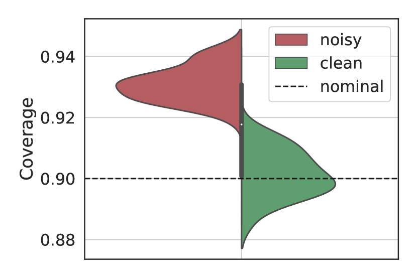
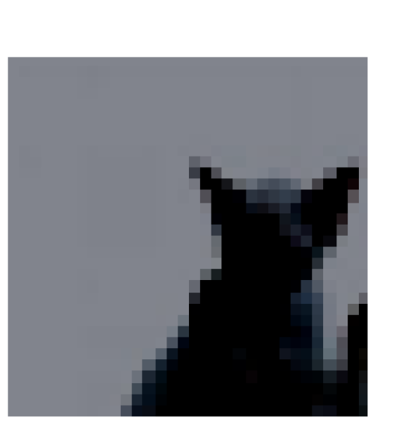
• True label:
   Cat

• Noisy:
  {Cat, Dog}

• Clean:
  {Cat}

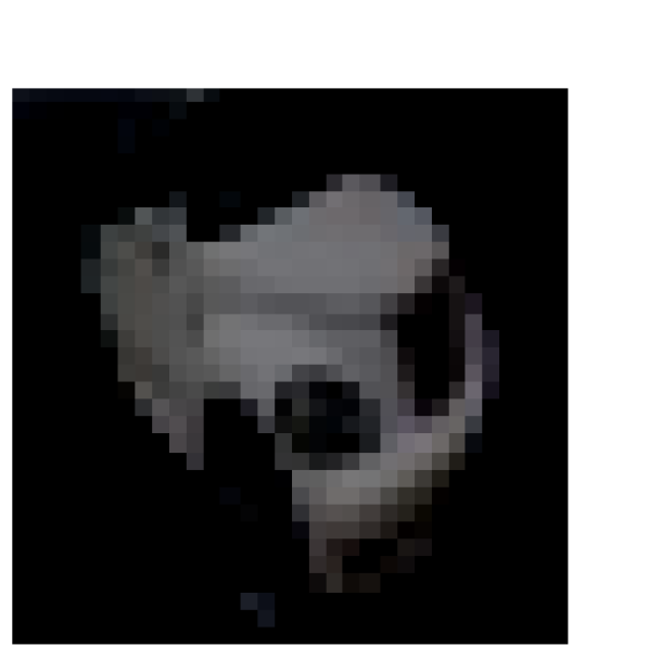
• True label:
   Car

• Noisy:
  {Car, Ship, Cat}

• Clean:
  {Car}

Figure 1: Effect of label noise on CIFAR-10. Left: distribution of average coverage on a clean test set over 30 independent experiments with target coverage $1-\alpha=90\%$, using noisy and clean labels for calibration. We use a pre-trained resnet 18 model, which has Top-1 accuracy of 93% and 90% on the clean and noisy test set, respectively. The gray bar represents the interquartile range. Center and right: prediction sets achieved using noisy and clean labels for calibration.

Regression

In this section, we present a real-world application with a continuous response, using Aesthetic Visual Analysis (AVA) data set, first presented by Murray et al. (2012). This data set contains pairs of images and their aesthetic scores in the range of 1 to 10, obtained by approximately 200 annotators. Following Kao et al. (2015); Talebi and Milanfar (2018); Murray et al. (2012), the task is to predict the average aesthetic score of a given test image. Therefore, we consider the average aesthetic score taken over all annotators as the clean, ground truth response. The noisy response is the average aesthetic score taken over 10 randomly selected annotators only.

We examine the performance of conformal prediction using two different scores: the CQR score (Romano et al., 2019) and the residual magnitude score (Lei et al., 2018) defined as:

$$s^{\rm RM}(x,y)=\big{|}\hat{f}(x)-y\big{|}/\hat{u}(x),$$ (7)

where in our experiments we set $\hat{u}(x)=1$. We follow Talebi and Milanfar (2018) and take a transfer learning approach to fit the predictive model. Specifically, for feature extraction, we use a VGG-16 model—pre-trained on the ImageNet data set—whose last (deepest) fully connected layer is removed. Then, we feed the output of the VGG-16 model to a linear fully connected layer to predict the response. We trained two different models: a quantile regression model for CQR and a classic regression model for conformal with residual magnitude score. The models are trained on $34,000$ noisy samples, calibrated on $7,778$ noisy holdout points, and tested on $7,778$ clean samples. Further details regarding the training strategy are in Appendix A2.3.

Figure 2 portrays the marginal coverage and average interval length achieved using CQR and residual magnitude scores. As a point of reference, this figure also presents the performance of the two conformal methods when calibrated with a clean calibration set; as expected, the two perfectly attain 90% coverage. By constant, when calibrating the same predictive models with a noisy calibration set, the resulting prediction intervals tend to be wider and to over-cover the average aesthetic scores.

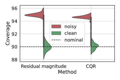
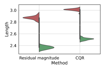
Figure 2: Results for real-data regression experiment: predicting aesthetic visual rating. Performance of conformal prediction intervals with 90% marginal coverage based on a VGG-16 model using a noisy training set. We compare the residual magnitude score and CQR methods with both noisy and clean calibration sets. Left: Marginal coverage; Right: Interval length. The results are evaluated over 30 independent experiments and the gray bar represents the interquartile range.

Thus far, we have found in empirical experiments that conservative coverage is obtained in the presence of label noise. In the following sections, our objective is to establish conditions that formally guarantee label-noise robustness.

2.3 Theoretical Analysis

2.3.1 General Analysis

We begin the theoretical analysis with a general statement, showing that Recipe 1 produces valid prediction sets whenever the noisy score distribution stochastically dominates the clean score distribution. The intuition is that the noise distribution ‘spreads out’ the distribution of the score function such that $\hat{q}_{\rm noisy}$ is (stochastically) larger than $\hat{q}_{\rm clean}$.

Theorem 2.1.

Assume that $\mathbb{P}(\tilde{s}_{\rm test}\leq t)\leq\mathbb{P}(s_{\rm test}\leq t)$ for all $t$. Then,

$$\mathbb{P}\left(Y_{\rm test}\in\widehat{\mathcal{C}}_{\rm noisy}(X_{\rm test})\right)\geq 1-\alpha.$$ (8)

Furthermore, for any $u$ satisfying $\mathbb{P}(\tilde{s}_{\rm test}\leq t)+u\geq\mathbb{P}(s_{\rm test}\leq t),$ for all $t$, then

$$\mathbb{P}\left(Y_{\rm test}\in\widehat{\mathcal{C}}_{\rm noisy}(X_{\rm test})\right)\leq 1-\alpha+\frac{1}{n+1}+u.$$ (9)

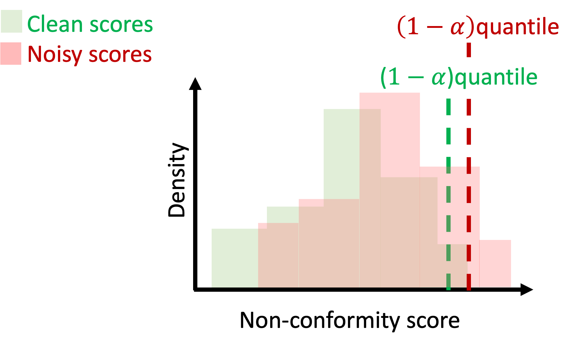
Figure 3: Clean (green) and noisy (red) non-conformity scores under dispersive corruption.

Figure 3 illustrates the idea behind Theorem 2.1, demonstrating that when the noisy score distribution stochastically dominates the clean score distribution, then $\hat{q}_{\rm noisy}\geq\hat{q}_{\rm clean}$ and thus uncertainty sets calibrated using noisy labels are more conservative. In practice, however, one does not have access to such a figure, since the scores of the clean labels are unknown. This gap requires an individual analysis for every task and its noise setup, which emphasizes the complexity of this study. In the following subsections, we present example setups in classification and regression tasks under which this stochastic dominance holds, and conformal prediction with noisy labels succeeds in covering the true, noiseless label. The purpose of these examples is to illustrate simple and intuitive statistical settings where Theorem 2.1 holds. Under the hood, all setups given in the following subsections are applications of Theorem 2.1. Though the noise can be adversarially designed to violate these assumptions and cause under-coverage (as in the impossibility result in Proposition 2.3), the evidence presented here suggests that in the majority of practical settings, conformal prediction can be applied without modification. All proofs are given in Appendix A1.

2.3.2 Regression

In this section, we analyze a regression task where the labels are continuous-valued and the corruption function is additive:

$$g^{\rm add}(y)=y+Z$$ (10)

for some independent noise sample $Z$.

We first analyze the setting where the noise $Z$ is symmetric around 0 and the density of $Y\mid X$ is symmetric unimodal. We also assume that the estimated prediction interval contains the true median of $\tilde{Y}\mid X=x$, which is an extremely weak assumption about the fitted model. The following proposition states that such an interval achieves a conservative coverage rate over the clean labels.

Proposition 2.1.

Let $\widehat{\mathcal{C}}_{\rm noisy}(X_{\rm test})$ be a prediction interval constructed according to Recipe 1 with the corruption function $g^{\rm add}$. Further, suppose that $\widehat{\mathcal{C}}_{\rm noisy}(x)$ contains the true median of $\tilde{Y}\mid X=x$ for all $x\in\mathcal{X}$. Then

$$\mathbb{P}\Big{(}Y_{\rm test}\in\widehat{\mathcal{C}}_{\rm noisy}(X_{\rm test})\Big{)}\geq 1-\alpha.$$ (11)

Importantly, the corruption function may depend on the feature vector, as stated next.

Remark 2.2 (Corruptions dependent on X).

Proposition 2.1 holds even if the noise $\epsilon$ depends on $X$.

Additionally, the distributional assumption on $Y\mid X$ is not necessary to guarantee label-noise robustness under this noise model; in Appendix A1.3 we show that this distributional assumption can be lifted at the expense of additional requirements on the estimated interval. Furthermore, in Section 3.3.3 we extend this analysis and formulate bounds for the coverage rate obtained on the clean labels that do not require any distributional assumptions and impose no restrictions on the constructed intervals. Subsequently, in Section 4.5, we empirically evaluate the proposed bounds and show that they are informative despite their extremely weak assumptions.

2.3.3 Classification

In this section, we formulate under which conditions conformal prediction is robust to label noise in a $K$-class classification setting where the labels take one of $K$ values, i.e., $Y\in\{1,2,...,K\}$. In a nutshell, robustness is guaranteed when the corruption function transforms the labels’ distribution towards a uniform distribution while maintaining the same ranking of labels. Such corruption increases the prediction uncertainty, which drives conformal methods to construct conservative uncertainty sets to achieve the nominal coverage level on the observed noisy labels. We now formalize this intuition.

Proposition 2.2.

Let $\widehat{\mathcal{C}}_{\rm noisy}$ be constructed as in Recipe 1 such that it contains the most likely labels, i.e., $\forall x\in\mathcal{X},i\in\widehat{\mathcal{C}}_{\rm noisy}(x),j\notin\widehat{\mathcal{C}}_{\rm noisy}(x):\mathbb{P}(\tilde{Y}_{\rm test}=i\mid X_{\rm test}=x)\geq\mathbb{P}(\tilde{Y}_{\rm test}=j\mid X_{\rm test}=x)$. Further suppose that for all $x\in\mathcal{X}$:

1. $\forall i\in\{1,..,K\}:\left|\mathbb{P}(\tilde{Y}_{\rm test}=i\mid X_{\rm test}=x)-\frac{1}{K}\right|\leq\left|\mathbb{P}(Y_{\rm test}=i\mid X_{\rm test}=x)-\frac{1}{K}\right|,$

2. $\forall i,j\in\{1,..,K\}:\mathbb{P}(Y_{\rm test}=i\mid X_{\rm test}=x)\leq\mathbb{P}(Y_{\rm test}=j\mid X_{\rm test}=x)\iff\mathbb{P}(\tilde{Y}_{\rm test}=i\mid X_{\rm test}=x)\leq\mathbb{P}(\tilde{Y}_{\rm test}=j\mid X_{\rm test}=x).$

Then, the coverage achieved over the clean labels is bounded by:

$$1-\alpha\leq\mathbb{P}\left({Y}_{\rm test}\in\widehat{\mathcal{C}}_{\rm noisy}(X_{\rm test})\right)\leq 1-\alpha+\frac{1}{n+1}+\frac{1}{2}\sum_{i=1}^{K}{\left|\mathbb{P}(\tilde{Y}_{\rm test}=i)-\mathbb{P}({Y}_{\rm test}=i)\right|}.$$ (12)

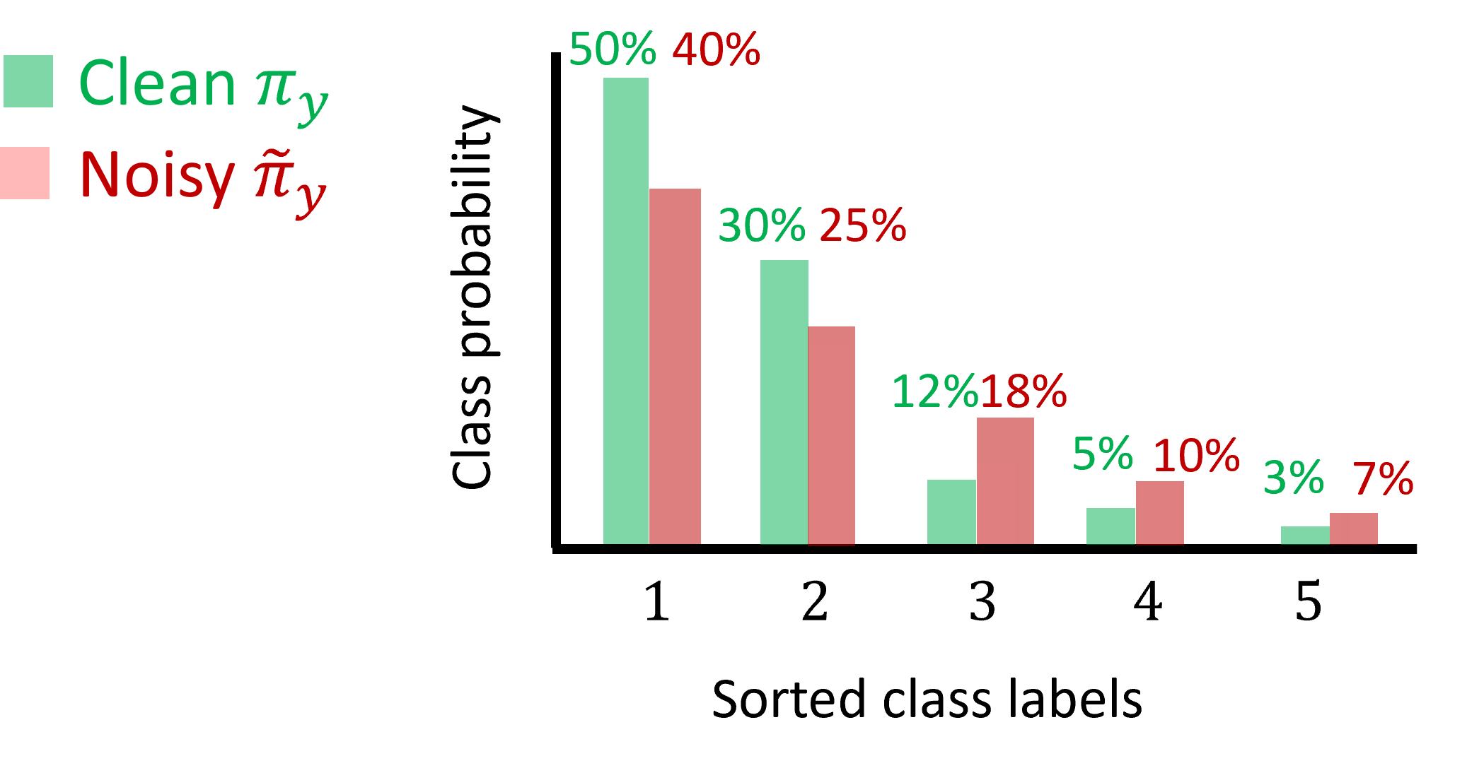
Figure 4: Clean (green) and noisy (red) class probabilities under dispersive corruption.

Figure 4 visualizes the essence of Proposition 2.2, showing that as the corruption increases the label uncertainty, the prediction sets generated by conformal prediction get larger, having a conservative coverage rate. It should be noted that under the above proposition, achieved valid coverage requires only knowledge of the noisy conditional distribution $\mathbb{P}\big{(}\tilde{Y}\;\mid\;X\big{)}$, so a model trained on a large amount of noisy data should approximately have the desired coverage rate. Moreover, one should notice that without the assumptions in Proposition 2.2, even the oracle model is not guaranteed to achieve valid coverage, as we will show in Section 4.1. For a more general analysis of classification problems where the noise model is an arbitrary confusion matrix, see Appendix A1.2.

We now turn to examine two conformity scores and show that applying them with noisy data leads to conservative coverage, as a result of Proposition 2.2. The adaptive prediction sets (APS) scores, first introduced by Romano et al. (2020), is defined as

$$s^{\rm APS}\left(x,y\right)=\sum_{y^{\prime}\in\mathcal{Y}}\hat{{\pi}}_{y^{\prime}}\left(x\right)\mathbb{I}\left\{\hat{{\pi}}_{y^{\prime}}\left(x\right)>\hat{{\pi}}_{y}\left(x\right)\right\}+\hat{{\pi}}_{y}\left(x\right)\cdot U^{\prime},$$ (13)

where $\mathbb{I}$ is the indicator function, $\hat{{\pi}}_{y}\left(x\right)$ is the estimated conditional probability $\mathbb{P}\big{(}Y=y\;\mid\;X=x\big{)}$ and $U^{\prime}\sim\mathrm{Unif}(0,1)$. To make this non-random, a variant of the above where $U^{\prime}=1$ is often used. The APS score is one of two popular conformal methods for classification. The other score from Vovk et al. (2005); Lei et al. (2013), is referred to as homogeneous prediction sets (HPS) score, $s^{\rm HPS}\left(x,y\right)=1-\hat{{\pi}}_{y}\left(x\right)$, for some classifier $\hat{{\pi}}_{y}\left(x\right)\in[0,1]$. The next corollary states that with access to an oracle classifier’s ranking, conformal prediction covers the noiseless test label.

Corollary 1.

Let $\widehat{\mathcal{C}}_{\rm noisy}(X_{\rm test})$ be constructed as in Recipe 1 with either the APS or HPS score functions, with any classifier that ranks the classes in the same order as the oracle classifier $\hat{{\pi}}_{y}(x)=\mathbb{P}\big{(}\tilde{Y}=y\;\mid\;X=x\big{)}$. Then

$$1-\alpha\leq\mathbb{P}\Big{(}Y_{\rm test}\in\widehat{\mathcal{C}}_{\rm noisy}(X_{\rm test})\Big{)}\leq 1-\alpha+\frac{1}{n+1}+\frac{1}{2}\sum_{i=1}^{K}{\left|\mathbb{P}(\tilde{Y}_{\rm test}=i)-\mathbb{P}({Y}_{\rm test}=i)\right|}.$$ (14)

We now turn to examine a specific noise model in which the noisy label is randomly flipped $\epsilon$ fraction of the time. This noise model is well-studied in the literature; see, for example, (Aslam and Decatur, 1996; Angluin and Laird, 1988; Ma et al., 2018; Jenni and Favaro, 2018; Jindal et al., 2016; Yuan et al., 2018). Formally, we define the corruption model as follows:

$$g^{\rm flip}(y)=\begin{cases}y&\text{w.p }1-\epsilon\\ Y^{\prime}&\text{else},\end{cases}$$ (15)

where $Y^{\prime}$ is uniformly drawn from the set $\{1,...,K\}$. Under the random flip noise model, we get the following coverage upper bound.

Corollary 2.

Let $\widehat{\mathcal{C}}_{\rm noisy}(X_{\rm test})$ be constructed as in Recipe 1 with the corruption function $g^{\rm flip}$ and either the APS or HPS score functions, with any classifier that ranks the classes in the same order as the oracle classifier $\hat{{\pi}}_{y}(x)=\mathbb{P}\big{(}\tilde{Y}=y\;\mid\;X=x\big{)}$. Then

$$1-\alpha\leq\mathbb{P}\Big{(}Y_{\rm test}\in\widehat{\mathcal{C}}_{\rm noisy}(X_{\rm test})\Big{)}\leq 1-\alpha+\frac{1}{n+1}+\epsilon\frac{K-1}{K}.$$ (16)

Crucially, the above corollaries apply with any score function that preserves the order of the estimated classifier, which emphasizes the generity of our theory. Finally, we note that in Section 3.3.1 we extend the above analysis to multi-label classification, where there may be multiple labels that correspond to the same sample.

2.4 Disclaimer: Distribution-Free Results

Though the coverage guarantee holds in many realistic cases, conformal prediction may generate uncertainty sets that fail to cover the true outcome. Indeed, in the general case, conformal prediction produces invalid prediction sets, and must be adjusted to account for the size of the noise. The following proposition states that for any nontrivial noise distribution, there exists a score function that breaks naïve conformal.

Proposition 2.3 (Coverage is impossible in the general case.).

Take any $\tilde{Y}\overset{d}{\neq}Y$. Then there exists a score function $s$ that yields $\mathbb{P}\left(Y_{\rm test}\in\widehat{\mathcal{C}}_{\rm noisy}(X_{\rm test})\right)<\mathbb{P}\left(Y_{\rm test}\in\widehat{\mathcal{C}}(X_{\rm test})\right)$, for $\widehat{\mathcal{C}}_{\rm noisy}$ constructed using noisy samples and $\widehat{\mathcal{C}}$ constructed with clean samples.

The above proposition says that for any noise distribution, there exists an adversarially chosen score function that will disrupt coverage. Furthermore, as we discuss in Appendix A1, with a noise of a sufficient magnitude, it is possible to get arbitrarily bad violations of coverage.

Next, we discuss how to adjust the threshold of conformal prediction to account for noise of a known size, as measured by total variation (TV) distance from the clean label.

Corollary 3 (Corollary of Barber et al. (2022)).

Let $\tilde{Y}$ be any random variable satisfying $D_{\rm TV}(Y,\tilde{Y})\leq\epsilon$. Take $\alpha^{\prime}=\alpha+2\frac{n}{n+1}\epsilon$. Letting $\widehat{\mathcal{C}}_{\rm noisy}(X_{\rm test})$ be the output of Recipe 1 with any score function at level $\alpha^{\prime}$ yields

$$\mathbb{P}\big{(}Y_{\rm test}\in\widehat{\mathcal{C}}_{\rm noisy}(X_{\rm test})\big{)}\geq 1-\alpha.$$ (17)

We discuss this strategy more in Appendix A1—the algorithm implied by Corollary 3 may not be particularly useful, as the TV distance is a badly behaved quantity that is also difficult to estimate, especially since the clean labels are inaccessible.

As a final note, if the noise is bounded in TV norm, then the coverage is also not too conservative.

Corollary 4 (Corollary of Barber et al. (2022) Theorem 3).

Let $\tilde{Y}$ be any random variable satisfying $D_{\rm TV}(Y,\tilde{Y})\leq\xi$. Letting $\widehat{\mathcal{C}}_{\rm noisy}(X_{\rm test})$ be the output of Recipe 1 with any score function at level $\alpha$ yields

$$\mathbb{P}\big{(}Y_{\rm test}\in\widehat{\mathcal{C}}_{\rm noisy}(X_{\rm test})\big{)}<1-\alpha+\frac{1}{n+1}+\frac{n}{n+1}\xi.$$ (18)

3 Risk Control Under Label Noise

3.1 Background

Up to this point, we have focused on the miscoverage loss, and the analysis conducted thus far applies exclusively to this metric. However, in real-world applications, it is often desired to control metrics other than the binary loss $L^{\text{miscoverage}}(y,C)=\mathbbm{1}\{y\notin C\}$. Examples of such alternative losses include the F1-score or the false negative rate. The latter is particularly relevant for high-dimensional response $Y$, as in tasks like multi-label classification or image segmentation. To address this need, researchers have developed extensions of the conformal framework that go beyond the 0-1 loss, providing a rigorous risk control guarantee over general loss functions (Bates et al., 2021; Angelopoulos et al., 2021, 2022). Specifically, these techniques take a loss function $L$ that measures the error of the estimated predictions and generate uncertainty sets with a risk controlled at pre-specified level $\alpha$:

$$\mathcal{R}(C)=\mathbb{E}[L(Y_{\rm test},\widehat{\mathcal{C}}(X_{\rm test})]\leq\alpha.$$ (19)

Analogously to conformal prediction, these methods produce valid sets under the i.i.d. assumption, but their guarantees do not hold in the presence of label noise. Nevertheless, in the next section, we conduct a real-data experiment, demonstrating that conformal risk control is robust to label noise. In the following sections, we aim to explain this phenomenon and find the conditions under which conservative risk is obtained.

3.2 Empirical Evidence

Multi-label Classification

In this section, we analyze the robustness of conformal risk control (Angelopoulos et al., 2022) to label noise in a multi-label classification setting. We use the MS COCO dataset (Lin et al., 2014), in which the input image may contain up to $K=80$ positive labels, i.e., $Y\subseteq\{1,2,...,K\}$. In the following experiment, we consider the annotations in this dataset as ground-truth labels. We have collected noisy labels from individual annotators who annotated 117 images in total. On average, the annotators missed or mistakenly added approximately 1.75 labels from each image. See Appendix A2.5 for additional details about this experimental setup and data collection.

We fit a TResNet (Ridnik et al., 2021) model on 100k clean samples and calibrate it using 105 noisy samples with conformal risk control, as introduced in (Angelopoulos et al., 2022, Section 3.2), to control the false-negative rate (FNR) at different levels. The FNR is the ratio of positive labels that are missed in the prediction sets, formally defined as:

$$L^{\rm FNR}(Y,C)=1-\frac{|Y\cap C|}{|Y|}.$$ (20)

We measure the FNR obtained over the clean and noisy test sets which contain 40k and 12 samples, respectively. Figure 5 displays the results, showing that the uncertainty sets attain valid risk even though they were calibrated using corrupted data. In the following section, we aim to explain these results and find the conditions under which label-noise robustness is guaranteed.

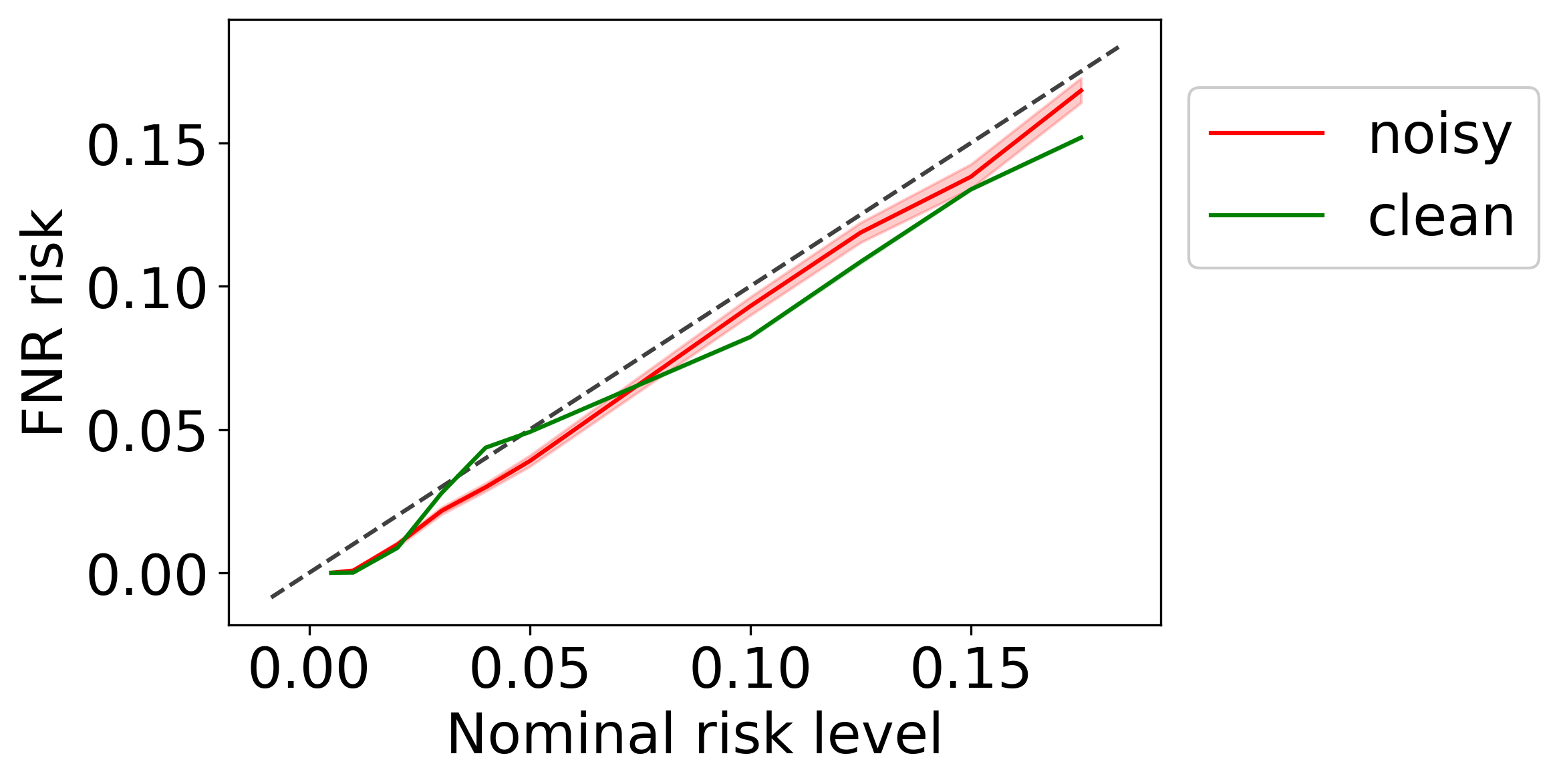
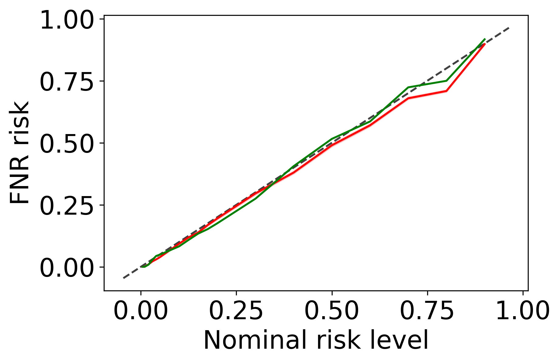
Figure 5: FNR on MS COCO dataset, achieved over noisy (red) and clean (green) test sets. The calibration scheme is applied with noisy annotations. Results are averaged over 2000 trials.

3.3 Theoretical Analysis

3.3.1 Multi-label Classification

In this section, we study the conditions under which conformal risk control is robust to label noise in a multi-label classification setting. Recall that each sample contains up to $K$ positive labels, i.e., $Y\subseteq\{1,2,...,K\}$. Here, we assume a vector-flip noise model with a binary random variable $\epsilon_{i}$ that flips the $i$-th label with probability $\mathbb{P}(\epsilon_{i}=1)$:

$$g^{\rm vector-flip}(y)_{i}=y_{i}(1-\epsilon_{i})+(1-y_{i})\epsilon_{i}.$$ (21)

Above, $y_{i}$ is an indicator that takes 1 if the $i$-th label is present in $y$, and 0, otherwise. Notice that the random variable $\epsilon_{i}$ takes the value 1 if the $i$-th label in $y$ is flipped and 0 otherwise. We further assume that the noise is not adversarial, i.e., $\mathbb{P}(\epsilon_{i}=1)<0.5$ for all $i\in\{1,2,...,K\}$. We now show that a valid FNR risk is guaranteed in the presence of label noise under the following assumptions.

Proposition 3.1.

Let $\widehat{\mathcal{C}}_{\rm noisy}(X_{\rm test})$ be a prediction set that contains the most likely labels and controls the FNR risk of the noisy labels at level $\alpha$. Assume the multi-label noise model $g^{\rm vector-flip}$. If

1. $Y_{\rm test}$ is a deterministic function of $X_{\rm test}$,

2. $|\tilde{Y}_{\rm test}|\mid X_{\rm test}=x$ is a constant for all $x\in\mathcal{X}$,

then

$$\mathbb{E}\left[L^{\rm FNR}\left(Y_{\rm test},\widehat{\mathcal{C}}_{\rm noisy}(X_{\rm test})\right)\right]\leq\alpha.$$ (22)

Remark 3.1 (Dependent corruptions).

Proposition 3.1 holds even if the elements in the noise vector $\epsilon$ depend on each other or on $X$.

Importantly, the determinism assumption on $Y\mid X=x$ is reasonable as it is simply satisfied when the noiseless response is defined as the consensus outcome. Nevertheless, this assumption may not always hold in practice. Thus, in the next section, we propose alternative requirements for the validity of the FNR risk and demonstrate them in a segmentation setting.

3.3.2 Segmentation

In segmentation tasks, the goal is to assign labels to every pixel in an input image such that pixels with similar characteristics share the same label. For example, tumor segmentation can be applied to identify polyps in medical images. Here, the response is a binary matrix $Y\subseteq\{0,1\}^{W\times H}$ that contains the value $1$ in the $(i,j)$ pixel if it includes the object of interest and $0$ otherwise. The uncertainty is represented by a prediction set $C\subseteq\{1,...,W\}\times\{1,...,H\}$ that includes pixels that are likely to contain the object. Similarly to the multi-label classification problem, here, we assume a vector flip noise model $g^{\rm vector-flip}$, that flips the $(i,j)$ pixel in $Y$, denoted as $Y_{i,j}$, with probability $\mathbb{P}(\epsilon_{i,j}=1)$. We now show that the prediction sets constructed using a noisy calibration set are guaranteed to have conservative FNR if the clean response matrix $Y$ and the noise variable $\epsilon$ are independent given $X$.

Proposition 3.2.

Let $\widehat{\mathcal{C}}_{\rm noisy}(X_{\rm test})$ be a prediction set that contains the most likely labels and controls the FNR risk of the noisy labels at level $\alpha$. Suppose that:

1. The elements of the clean response matrix are independent of each other given $X_{\rm test}$.

2. For a given input $X_{\rm test}$, the noise level of all response elements is the same.

3. The noise variable $\epsilon$ is independent of $Y_{\rm test}\mid X_{\rm test}=x$, and the noises of different labels are independent of each other given $X_{\rm test}$.

Then,

$$\mathbb{E}\left[L^{\rm FNR}\left(Y_{\rm test},\widehat{\mathcal{C}}_{\rm noisy}(X_{\rm test})\right)\right]\leq\alpha.$$ (23)

We note that a stronger version of this proposition that allows dependence between the elements in $Y_{\rm test}$ is given in Appendix A1.8.1, along with the proofs of these results. The advantage of Proposition 3.2 over Proposition 3.1 is that here, the response matrix $Y_{\rm test}$ and the number of positive labels are allowed to be stochastic. For this reason, we believe that Proposition 3.2 is more suited for segmentation tasks, even though Proposition 3.1 applies in segmentation settings as well.

3.3.3 Regression with a General Loss

This section studies the general regression setting in which $Y\in\mathbb{R}$ takes continuous values and the loss function is an arbitrary function $L(y,\widehat{\mathcal{C}}_{\rm noisy}(x))\in\mathbb{R}$. Here, our objective is to find tight bounds for the risk over the clean labels using the risk observed over the corrupted labels. The main result of this section accomplishes this goal while making minimal assumptions on the loss function, the noise model, and the data distribution.

Proposition 3.3.

Let $\widehat{\mathcal{C}}_{\rm noisy}(X_{\rm test})$ be a prediction interval that controls the risk at level $\alpha:=\mathbb{E}\left[L(\tilde{Y}_{\rm test},\widehat{\mathcal{C}}_{\rm noisy}(X_{\rm test})\right]$. Suppose that the second derivative of the loss $L(y;C)$ is bounded for all $y,C$: $q\leq\frac{\partial^{2}}{\partial y^{2}}L(y;C)\leq Q$ for some $q,Q\in\mathbb{R}$. If the labels are corrupted by the function $g^{\rm add}$ from (10) with a noise $Z$ that satisfies $\mathbb{E}[Z]=0$, then

$$\begin{split}\alpha-\frac{1}{2}QVar(Z)\leq\mathbb{E}\left[L(Y_{\rm test},\widehat{\mathcal{C}}_{\rm noisy}(X_{\rm test})\right]\leq\alpha-\frac{1}{2}qVar(Z).\end{split}$$ (24)

If we further assume that $L$ is convex then we obtain valid risk:

$$\mathbb{E}\left[L(Y_{\rm test},\widehat{\mathcal{C}}_{\rm noisy}(X_{\rm test})\right]\leq\alpha.$$ (25)

The proof is detailed in Appendix A1.4. Remarkably, Proposition 3.3 applies for every model, calibration scheme, distribution of $Y\mid X$, and loss function that is twice differentiable. The only requirement is that the noise must be additive and with mean 0. We now demonstrate this result on a smooth approximation of the miscoverage loss, formulated as:

$$L^{sm}(y,[a,b])=\frac{2}{1+e^{-\left(2\frac{y-a}{b-a}-1\right)^{2}}}$$ (26)

Corollary 5.

Let $\widehat{\mathcal{C}}_{\rm noisy}(X_{\rm test})$ be a prediction interval. Denote the smooth miscoverage over the noisy labels as $\alpha:=\mathbb{E}\left[L^{sm}(\tilde{Y}_{\rm test},\widehat{\mathcal{C}}_{\rm noisy}(X_{\rm test})\right]$. Under the assumptions of Proposition 3.3, the risk of the clean labels is bounded by

$$\alpha-\frac{1}{2}QVar(Z)\leq\mathbb{E}\left[L^{sm}(Y_{\rm test},\widehat{\mathcal{C}}_{\rm noisy}(X_{\rm test})\right]\leq\alpha-\frac{1}{2}qVar(Z),$$ (27)

where $q=\mathbb{E}_{X}\left[\min_{y}{{\frac{\partial^{2}}{\partial y^{2}}L^{sm}}(y,\widehat{\mathcal{C}}_{\rm noisy}(X))}\right]$ and $Q=\mathbb{E}_{X}\left[\max_{y}{{\frac{\partial^{2}}{\partial y^{2}}L^{sm}}(y,\widehat{\mathcal{C}}_{\rm noisy}(X))}\right]$ are known constants.

We now build upon Corollary 5 and establish a lower bound for the coverage rate achieved by intervals calibrated with corrupted labels.

Proposition 3.4.

Let $\widehat{\mathcal{C}}_{\rm noisy}(X_{\rm test})$ be a prediction interval. Suppose that the labels are corrupted by the function $g^{\rm add}$ from (10) with a noise $Z$ that satisfies $\mathbb{E}[Z]=0$, then

$$\mathbb{P}\Big{(}Y_{\rm test}\in\widehat{\mathcal{C}}_{\rm noisy}(X_{\rm test})\Big{)}\geq 1-\frac{\mathbb{E}[L^{\rm sm}(\tilde{Y}_{\rm test},\widehat{\mathcal{C}}_{\rm noisy}(X_{\rm test}))]-0.5PVar(Z)}{Q},$$ (28)

where $P,Q$ are tunable constants.

In Appendix A1.5 we give additional details about this result as well as formulate a stronger version of it that provides a tighter coverage bound. Finally, in Appendix A1.6 we provide an additional miscoverage bound which is more informative and tight for smooth densities of $Y\mid X=x$.

3.3.4 Online Learning

In this section, we focus on an online learning setting and show that all theoretical results presented thus far also apply to the online framework. Here, the data is given as a stream ${(X_{t},\tilde{Y}_{t})}_{t\in\mathbb{N}}$ in a sequential fashion. Importantly, we have access only to the noisy labels $\tilde{Y}_{t}$, and the clean labels $Y_{t}$ are unavailable throughout the entire learning process. At time stamp $t\in\mathbb{N}$, our goal is to construct a prediction set $\widehat{\mathcal{C}}_{\rm noisy}^{t}$ given on all previously observed samples ${(X_{t^{\prime}},\tilde{Y}_{t^{\prime}})}_{t^{\prime}=1}^{t-1}$ along with the test feature vector $X_{t}$ that achieves a long-range risk controlled at a user-specified level $\alpha$.

$$\mathcal{R}(\widehat{\mathcal{C}})=\lim_{T\to\infty}\frac{1}{T}\sum_{t=1}^{T}{L(Y_{t},\widehat{\mathcal{C}}_{\rm noisy}^{t}(X_{t}))}=\alpha.$$ (29)

There have been developed calibration schemes that generate uncertainty sets with statistical guarantees in online settings in the sense of 29. A popular one is Adaptive conformal inference (ACI), proposed by Gibbs and Candes (2021), which is an innovative online calibration scheme that constructs prediction sets with a pre-specified coverage rate, in the sense of (29) with the choice of the miscoverage loss. In contrast to ACI, Rolling risk control (Rolling RC) (Feldman et al., 2022) extends ACI by providing a guaranteed control of a general risk that may go beyond the binary loss. Yet, the guarantees of these approaches are invalidated when applied using corrupted data. Nonetheless, we argue that uncertainty sets constructed using corrupted data attain conservative risk in online settings under the requirements for offline label-noise robustness presented thus far.

Proposition 3.5.

Suppose that for all $t\in\mathbb{N}$ and $x\in\mathcal{X}$ we have a conservative loss:

$$\mathbb{E}\left[L\left(Y_{t},\widehat{\mathcal{C}}_{\rm noisy}^{t}(X_{t})\right)\middle|X_{t}=x\right]\leq\mathbb{E}\left[L\left(\tilde{Y}_{t},\widehat{\mathcal{C}}_{\rm noisy}^{t}(X_{t})\right)\middle|X_{t}=x\right].$$ (30)

Then:

$$\lim_{T\rightarrow\infty}{\frac{1}{T}\sum_{t=1}^{T}{L(Y_{t},\widehat{\mathcal{C}}_{\rm noisy}^{t}(X_{t}))}}\leq\alpha,$$ (31)

where $\alpha$ is the risk computed over the noisy labels.

The proof is given in Appendix A1.9. In words, Proposition 3.5 states that if the expected loss at every timestamp is conservative, then the risk over long-range windows in time is guaranteed to be valid. Practically, this proposition shows that all theoretical results presented thus far apply also in the online learning setting. We now demonstrate this result in two settings: online classification and segmentation and show that valid risk is obtained under the assumptions of Proposition 2.2 and Proposition 3.2, respectively.

Corollary 6 (Valid risk in online classification settings).

Suppose that the distributions of $Y_{t}\mid X_{t}$ and $\tilde{Y}_{t}\mid X_{t}$ satisfy the assumptions in Proposition 2.2 for all $t\in\mathbb{N}$. If $\widehat{\mathcal{C}}_{\rm noisy}^{t}(x)$ contains the most likely labels for every $t\in\mathbb{N}$ and $x\in\mathcal{X}$, then

$$\lim_{T\rightarrow\infty}{\frac{1}{T}\sum_{t=1}^{T}{\mathbbm{1}\{Y_{t}\notin\widehat{\mathcal{C}}_{\rm noisy}^{t}(X_{t})\}}}\leq\alpha.$$ (32)

Corollary 7 (Valid risk in online segmentation settings).

Suppose that the distributions of $Y_{t}\mid X_{t}$ and $\tilde{Y}_{t}\mid X_{t}$ satisfy the assumptions in Proposition 3.2 for all $t\in\mathbb{N}$. If $\widehat{\mathcal{C}}_{\rm noisy}^{t}(x)$ contains the most likely labels for every $t\in\mathbb{N}$ and $x\in\mathcal{X}$ then

$$\lim_{T\rightarrow\infty}{\frac{1}{T}\sum_{t=1}^{T}{L^{\text{FNR}}(Y_{t},\widehat{\mathcal{C}}_{\rm noisy}^{t}(X_{t}))}}\leq\alpha.$$ (33)

Finally, in Appendix A1.10 we analyze the effect of label noise on the miscoverage counter loss (Feldman et al., 2022). This loss assesses conditional validity in online settings by counting occurrences of consecutive miscoverage events. In a nutshell, Proposition A6 claims that with access to corrupted labels, the miscoverage counter is valid when the miscoverage risk is valid. This result is fascinating, as it connects the validity of the miscoverage counter to the validity of the miscoverage loss, where the latter is guaranteed under the conditions established in Section 2.3.

4 Experiments

4.1 Synthetic classification

In this section, we focus on multi-class classification problems, where we study the validity of conformal prediction using different types of label noise distributions, described below.

Class-independent noise.

This noise model, which we call uniform flip, randomly flips the ground truth label into a different one with probability $\epsilon$. Notice that this noise model slightly differs from the random flip $g^{\text{flip}}$ from (15), since in this uniform flip setting, a label cannot be flipped to the original label. Nonetheless, Proposition 2.2 states that the coverage achieved by an oracle classifier is guaranteed to increase in this setting as well.

Class-dependent noise.

In contrast to uniform flip noise, here, we consider a more challenging setup in which the probability of a label to be flipped depends on the ground truth class label $Y$. Such a noise label is often called Noisy at Random (NAR) in the literature, where certain classes are more likely to be mislabeled or confused with similar ones. Let $T$ be a row stochastic transition matrix of size $K\times K$ such that $T_{i,j}$ is the probability of a point with label $i$ to be swapped with label $j$. In what follows, we consider three possible strategies for building the transition matrix $T$. (1) Confusion matrix (Algan and Ulusoy, 2020): we define $T$ as the oracle classifier’s confusion matrix, up to a proper normalization to ensure the total flipping probability is $\epsilon$. We provide a theoretical study of this case in Appendix A1.2. (2) Rare to most frequent class (Xu et al., 2019): here, we flip the labels of the least frequent class with those of the most frequent class. This noise model is not uncommon in medical applications: imagine a setting where only a small fraction of the observations are abnormal, and thus likely to be annotated as the normal class. If switching between the rare and most frequent labels does not lead to a total probability of $\epsilon$, we move to the next least common class, and so on.

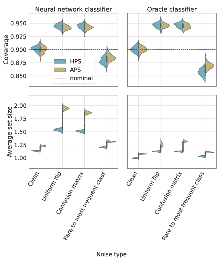
Figure 6: Effect of label noise on synthetic multi-class classification data. Performance of conformal prediction sets with target coverage $1-\alpha=90\%$, using a noisy training set and a noisy calibration set. Top: Marginal coverage; Bottom: Average size of predicted sets. The results are evaluated over 100 independent experiments and the gray bar represents the interquartile range.

To set the stage for the experiments, we generate synthetic data with $K=10$ classes as follows. The features $X\in\mathbb{R}^{d}$ follow a standard multivariate Gaussian distribution of dimension $d=100$. The conditional distribution of $Y\mid X$ is multinomial with weights $w_{j}(x)=\exp((x^{\top}B)_{j})/\sum_{i=1}^{K}\exp((x^{\top}B)_{i})$, where $B\in\mathbb{R}^{d\times K}$ whose entries are sampled independently from the standard normal distribution. In our experiments, we generate a total of $60,000$ data points, where $50,000$ are used to fit a classifier, and the remaining ones are randomly split to form calibration and test sets, each of size $5,000$. The training and calibration data are corrupted using the label noise models we defined earlier, with a fixed flipping probability of $\epsilon=0.05$. Of course, the test set is not corrupted and contains the ground truth labels. We apply conformal prediction using both the HPS and the APS score functions, with a target coverage level $1-\alpha$ of $90\%$. We use two predictive models: a two-layer neural network and an oracle classifier that has access to the conditional distribution of $\tilde{Y}\mid X$. Finally, we report the distribution of the coverage rate as in (2) and the prediction set sizes across $100$ random splits of the calibration and test data. As a point of reference, we repeat the same experimental protocol described above on clean data; in this case, we do not violate the i.i.d. assumption required to grant the marginal coverage guarantee in (1).

The results are depicted in Figure 6. As expected, in the clean setting all conformal methods achieve the desired coverage of $90\%$. Under the uniform flip noise model, the coverage of the oracle classifier increases to around $94\%$, supporting our theoretical results from Section 2.3.3. The neural network model follows a similar trend. Although not supported by a theoretical guarantee, when corrupting the labels using the more challenging confusion matrix noise, we can see a conservative behavior similar to the uniform flip. By contrast, under the rare to most frequent class noise model, we can see a decrease in coverage, which is in line with our disclaimer from Section 2.4. Yet, observe how the APS score tends to be more robust to label noise than HPS, which emphasizes the role of the score function.

In Appendix A2.1 we provide additional experiments with adversarial noise models that more aggressively reduce the coverage rate. Such adversarial cases are more pathological and less likely to occur in real-world settings, unless facing a malicious attacker.

4.2 Regression

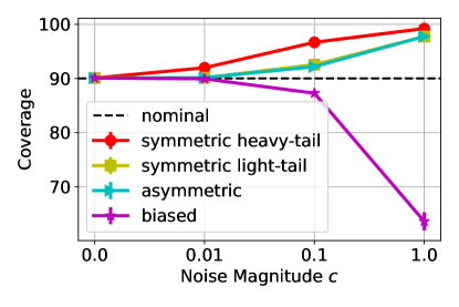
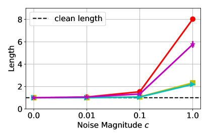
Figure 7: Response-independent noise. Performance of conformal prediction intervals with target coverage $1-\alpha=90\%$, using a noisy training set and a noisy calibration set. Left: Marginal coverage; Right: Length of predicted intervals (divided by the average clean length) using symmetric, asymmetric and biased noise with a varying magnitude. The results are evaluated over 50 independent experiments, with error bars showing one standard deviation. The standard deviation of $Y$ (without noise) and the square root of $\mathbb{E}\left[\textnormal{Var}\left[Y\mid X\right]\right]$ are both approximately 2.6.

Similarly to the classification experiments, we study two types of noise distributions.

Response-independent noise.

We consider an additive noise of the form: $\tilde{Y}=Y+c\cdot Z$, where $c$ is a parameter that allows us to control the noise level. The noise component $Z$ is a random variable sampled from the following distributions. (1) Symmetric light tailed: standard normal distribution; (2) Symmetric heavy tailed: t-distribution with one degree of freedom; (3) Asymmetric: standard gumbel distribution, normalized to have zero mean and unit variance; and (4) Biased: positive noise formulated as the absolute value of #2 above.

Response-dependent noise.

Analogously to the class-dependent noise from Section 4.1, we define more challenging noise models as follows. (1) Contractive: this corruption pushes the ground truth response variables towards their mean. Formally, $\tilde{Y}_{i}=Y_{i}-\left(Y_{i}-\frac{1}{n}\sum_{i=1}^{n}Y_{i}\right)\cdot U$, where $U$ is a random uniform variable defined on the segment [0,0.5], and $n$ is the number of calibration points. (2) Dispersive: this noise introduces some form of a dispersion effect on the ground truth response, which takes the opposite form of the contractive model, given by $\tilde{Y}_{i}=Y_{i}+\left(Y_{i}-\frac{1}{n}\sum_{i=1}^{n}Y_{i}\right)\cdot U$.

Having defined the noise models, we turn to describe the data-generating process. We simulate a 100-dimensional $X$ whose entries are sampled independently from a uniform distribution on the segment $[0,5]$. Following Romano et al. (2019), the response variable is generated as follows:

$$Y\sim\textrm{Pois}(\sin^{2}(\bar{X})+0.1)+0.03\cdot\bar{X}\cdot\eta_{1}+25\cdot\eta_{2}\cdot\mathbbm{1}\left\{U<0.01\right\},$$ (34)

where $\bar{X}$ is the mean of the vector $X$, and $\textrm{Pois}(\lambda)$ is the Poisson distribution with mean $\lambda$. Both $\eta_{1}$ and $\eta_{2}$ are i.i.d. standard Gaussian variables, and $U$ is a uniform random variable on $[0,1]$. The right-most term in (34) creates a few but large outliers. Figure A2 in the appendix illustrates the effect of the noise models discussed earlier on data sampled from (34).

We apply conformal prediction with the CQR score (Romano et al., 2019) for each noise model as follows. First, we fit a quantile random forest model on $8,000$ noisy training points; we then calibrate the model using $2,000$ fresh noisy samples; and, lastly, test the performance on additional $5,000$ clean, ground truth samples. The results are summarized in Figures 7 and  8. Observe how the prediction intervals tend to be conservative under symmetric, both for light- and heavy-tailed noise distributions, asymmetric, and dispersive corruption models. Intuitively, this is because these noise models increase the variability of $Y$; in Proposition 2.1 we prove this formally for any symmetric independent noise model, whereas here we show this result holds more generally even for response-dependent noise. By contrast, the prediction intervals constructed under the biased and contractive corruption models tend to under-cover the response variable. This should not surprise us: following Figure A2(c), the biased noise shifts the data ‘upwards’, and, consequently, the prediction intervals are undesirably pushed towards the positive quadrants. Analogously, the contractive corruption model pushes the data towards the mean, leading to intervals that are too narrow. Figure A5 in the appendix illustrates the scores achieved when using the different noise models and the 90%’th empirical quantile of the CQR scores. This figure supports the behavior witnessed in Figures 7, A3 and A4: over-coverage is achieved when $\hat{q}_{\rm noisy}$ is larger than $\hat{q}_{\rm clean}$, and under-coverage is obtained when $\hat{q}_{\rm noisy}$ is smaller.

In Appendix A2.2 we study the effect of the predictive model on the coverage property, for all noise models. To this end, we repeat similar experiments to the ones presented above, however, we now fit the predictive model on clean training data; the calibration data remains noisy. We also provide an additional adversarial noise model that reduces the coverage rate, but is unlikely to appear in real-world settings. Figures A3 and A4 in the appendix depict a similar behaviour for most noise models, except the biased noise for which the coverage requirement is not violated. This can be explained by the improved estimation of the low and high conditional quantiles, as these are fitted on clean data and thus less biased.

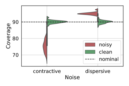
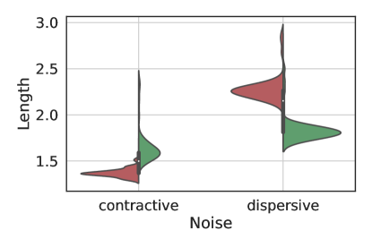
Figure 8: Dispersive versus contractive noise regression experiment. Performance of conformal prediction intervals with target coverage $1-\alpha=90\%$, using a noisy training set and a noisy calibration set. Left: Marginal coverage; Right: Length of predicted intervals. The results are evaluated over 50 independent experiments and the gray bar represents the interquartile range.

4.3 Multi-label classification

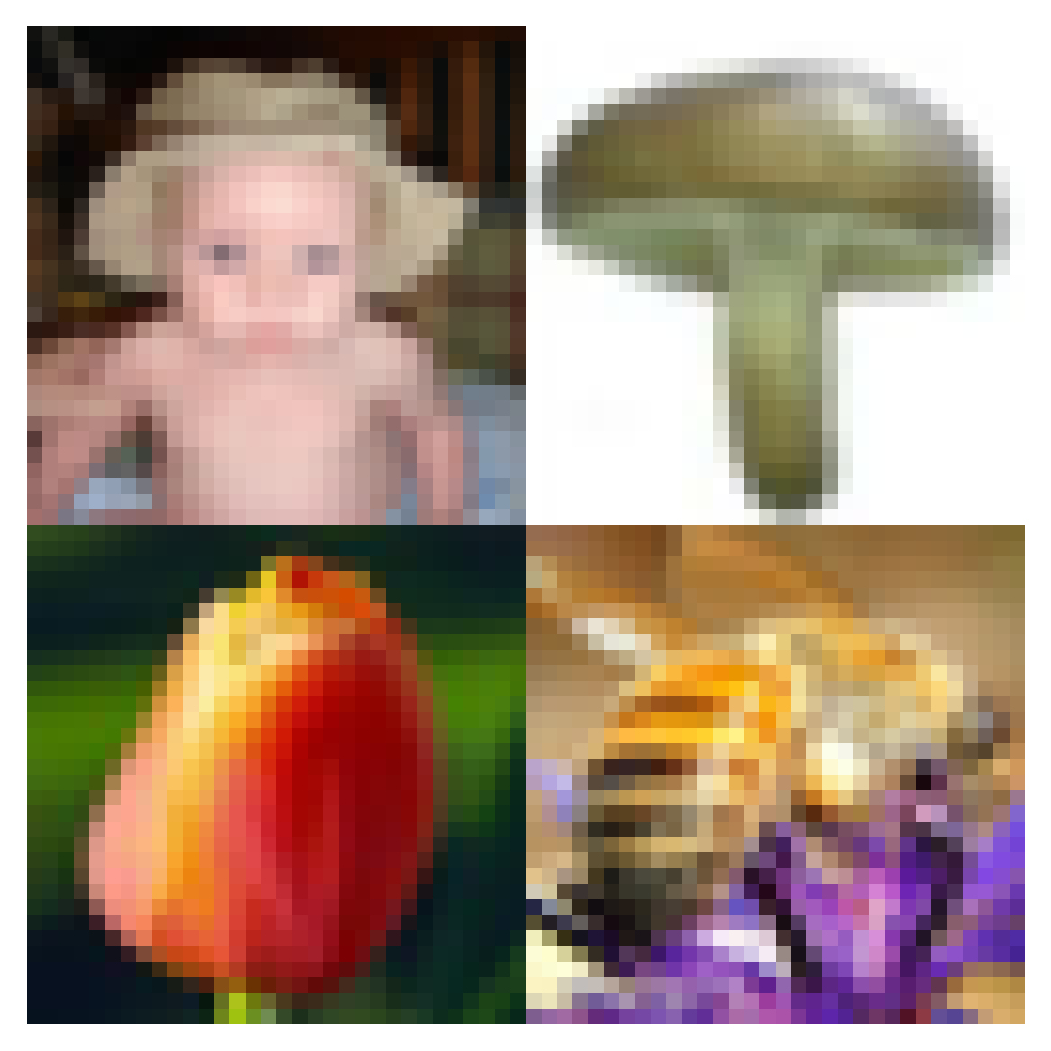
True labels:

baby, mushroom, tulip, bee.

Noisy labels:

baby, mushroom, sweet pepper, bee.

Figure 9: Visualization of the multi-label CIFAR-100N data.

In this section, we analyze conformal risk control in a multi-label classification task. For this purpose, we use the CIFAR-100N data set (Wei et al., 2022), which contains 50K colored images. Each image belongs to one of a hundred fine classes that are grouped into twenty mutually exclusive coarse super-classes. Furthermore, every image has a noisy and a clean label, where the noise rate of the fine categories is $40\%$ and of the coarse categories is $25\%$. We turn this single-label classification task into a multi-label classification task by merging four random images into a 2 by 2 grid. Every image is used once in each position of the grid, and therefore this new dataset consists of 50K images, where each is composed of four sub-images and thus associated with up to four labels. Figure 9 displays a visualization of this new variant of the CIFAR-100N dataset.

We fit a TResNet (Ridnik et al., 2021) model on 40k noisy samples and calibrate it using 2K noisy samples with conformal risk control, as outlined in (Angelopoulos et al., 2022, Section 3.2). We control the false-negative rate (FNR) defined in (20) at different levels and measure the FNR obtained over clean and noisy versions of the test set, which contains 8k samples. We conducted this experiment twice: once with the fine-classed labels and once with the super-classed labels. Figure 10 presents the results in both settings, showing that the risk obtained over the clean labels is valid for every nominal level. Importantly, this corruption setting violates the assumptions of Proposition 3.1, as the positive label count may vary across different noise instantiations. This experiment reveals that valid risk can be achieved in the presence of label noise even when the corruption model violates the requirements of our theory.

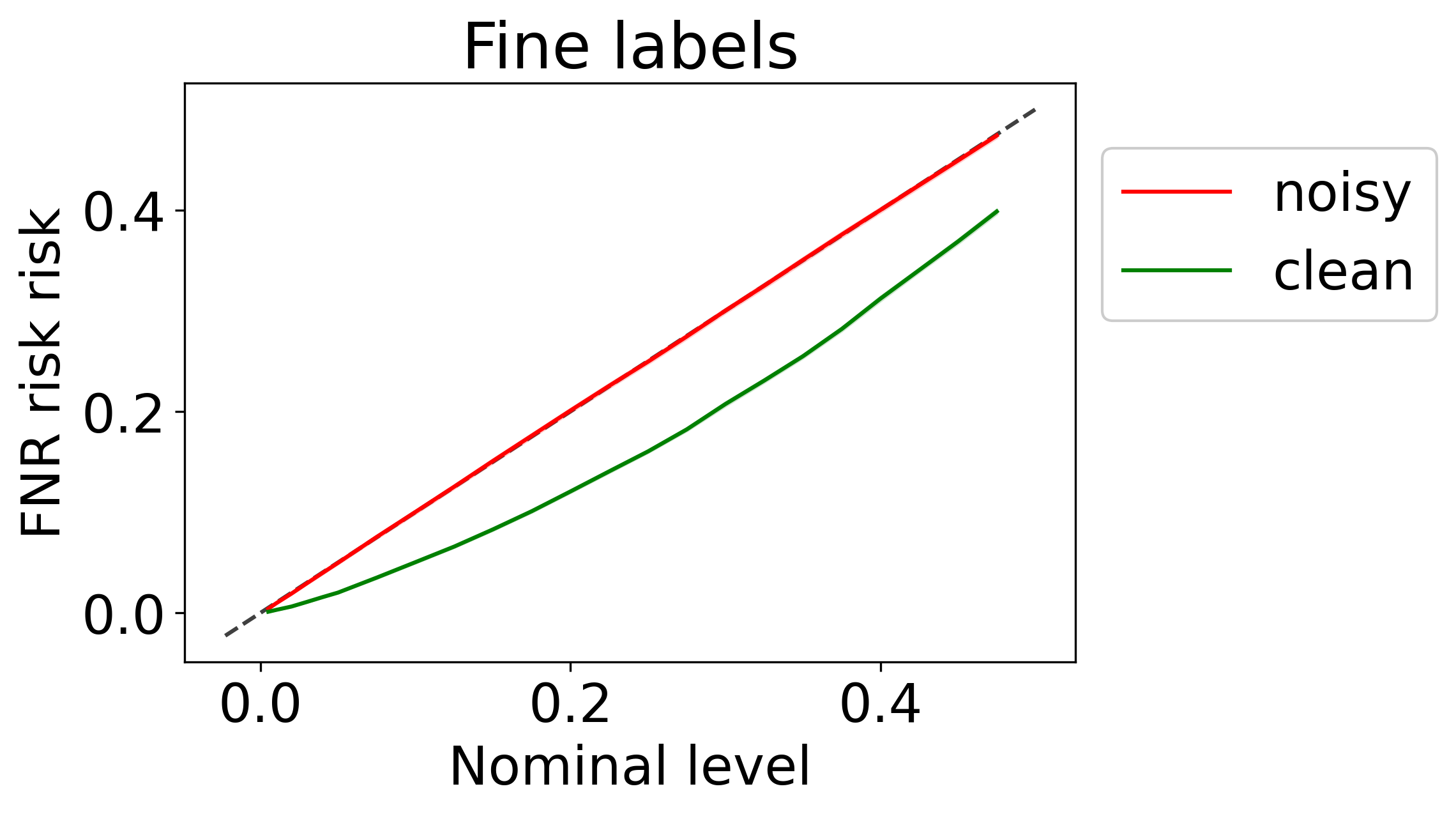
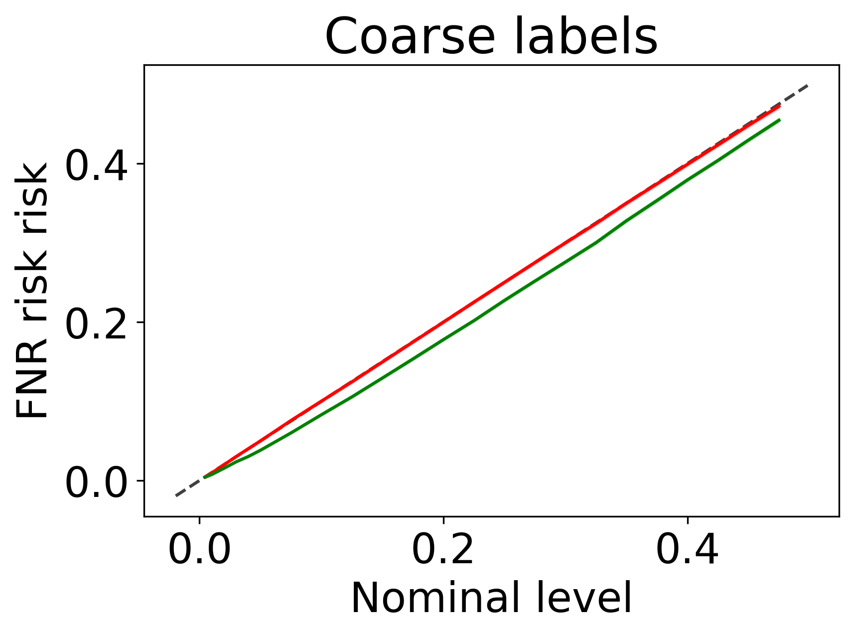
Figure 10: FNR achieved over noisy (red) and clean (green) test sets of the on CIFAR-100N dataset. Left: fine labels. Right: coarse labels. The calibration scheme is applied using noisy annotations in all settings. Results are averaged over 50 trials.

4.4 Segmentation

In this section, we follow a common artificial label corruption methodology, following Zhao and Gomes (2021); Kumar et al. (2020), and analyze three corruption setups that are special cases of the vector-flip noise model from (21): independent, dependent, and partial. In the independent setting, each pixel’s label is flipped with probability $\beta$, independently of the others. In the dependent setting, however, two rectangles in the image are entirely flipped with probability $\beta$, and the other pixels are flipped independently with probability $\beta$. Finally, in the partial noise setting, only one rectangle in the image is flipped with probability $\beta$, and the other pixels are unchanged.

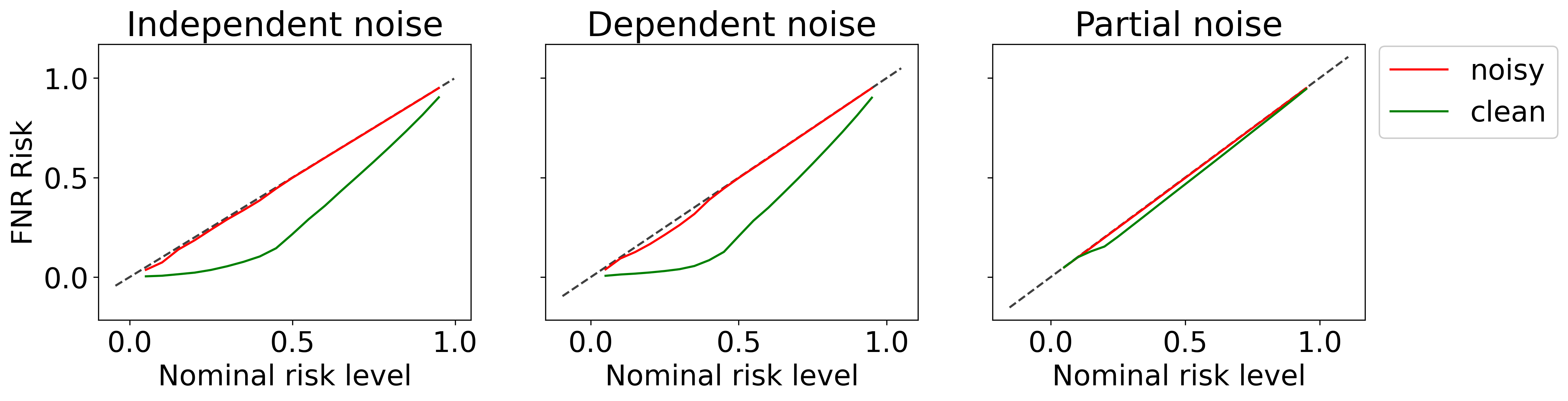
Figure 11: FNR on a polyp segmentation dataset, achieved over noisy (red) and clean (green) test sets. Left: independent noise. Middle: dependent noise. Right: partial noise. The predictive model is calibrated using noisy annotations in all settings, where the noise level is set to $\beta=0.1$. Results are averaged over 1000 trials.

We experiment on a polyp segmentation task, pooling data from several polyp datasets: Kvasir, CVC-ColonDB, CVC-ClinicDB, and ETIS-Larib. We consider the annotations given in the data as ground-truth labels and artificially corrupt them according to the corruption setups described above, to generate noisy labels. We use PraNet (Fan et al., 2020) as a base model and fit it over 1450 noisy samples. Then, we calibrate it using 500 noisy samples with conformal risk control, as outlined in (Angelopoulos et al., 2022, Section 3.2) to control the false-negative rate (FNR) from (20) at different levels. Finally, we evaluate the FNR over clean and noisy versions of the test set, which contains 298 samples, and report the results in Figure 11. This figure indicates that conformal risk control is robust to label noise, as the constructed prediction sets achieve conservative risk in all experimented noise settings. This is not a surprise, as it is guaranteed by Propositions 3.2 and A1.2.

4.5 Regression risk bounds

We now turn to demonstrate the coverage rate bounds derived in Section 3.3.3 on real and synthetic regression datasets. We examine two real benchmarks: meps_ (19) and bio , and one synthetic dataset that was generated from a bimodal density function with a sharp slope, as visualized in Figure 12. The simulated data was deliberately designed to invalidate the assumptions of our label-noise robustness requirements in Proposition 2.1. Consequentially, prediction intervals that do not cover the two peaks of the density function might undercover the true outcome, even if the noise is dispersive. Therefore, this gap calls for our distribution-free risk bounds which are applicable in this setup, in contrast to Proposition 2.1, and can be used to assess the worst risk level that may be obtained in practice.

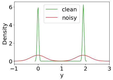
Figure 12: Visualization of the marginal density function of the adversarial synthetic data.

We consider the labels given in the real and synthetic datasets as ground truth and artificially corrupt them according to the additive noise model (10). The added noise is independently sampled from a normal distribution with mean zero and variance $0.1Var(Y)$. For each dataset and nominal risk level $\alpha$, fit a quantile regression model on 12K samples and learn the $\alpha/2,1-\alpha/2$ conditional quantiles of the noisy labels. Then, we calibrated its outputs using another 12K samples of the data with conformal risk control, by Angelopoulos et al. (2022), to control the smooth miscoverage (26) at level $\alpha$. Finally, we evaluate the performance on the test set which consists of 6K samples. We also compute the smooth miscoverage risk bounds according to Corollary 5 with a noise variance set to $0.1$. Figure 13 presents the risk bound along with the smooth miscoverage obtained over the clean and noisy versions of the test set. This figure indicates that conformal risk control generates invalid uncertainty sets when applied on the simulated noisy data, as we anticipated. Additionally, this figure shows that the proposed risk bounds are valid and tight, meaning that these are informative and effective. Moreover, this figure highlights the main advantage of the proposed risk bounds: their validity is universal across all distributions of the response variable and the noise component. Lastly, we note that in Appendix A2.7 we repeat this experiment with the miscoverage loss and display the miscoverage bound derived from Corollary 3.4.

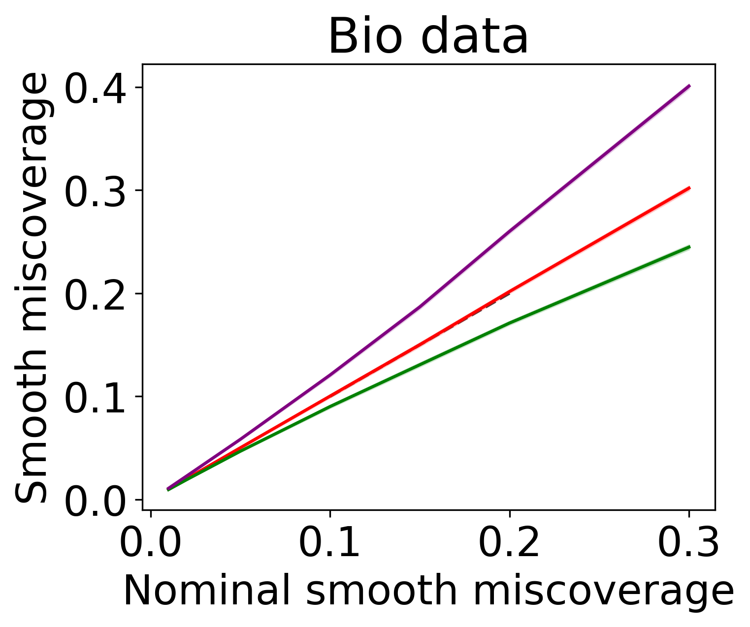
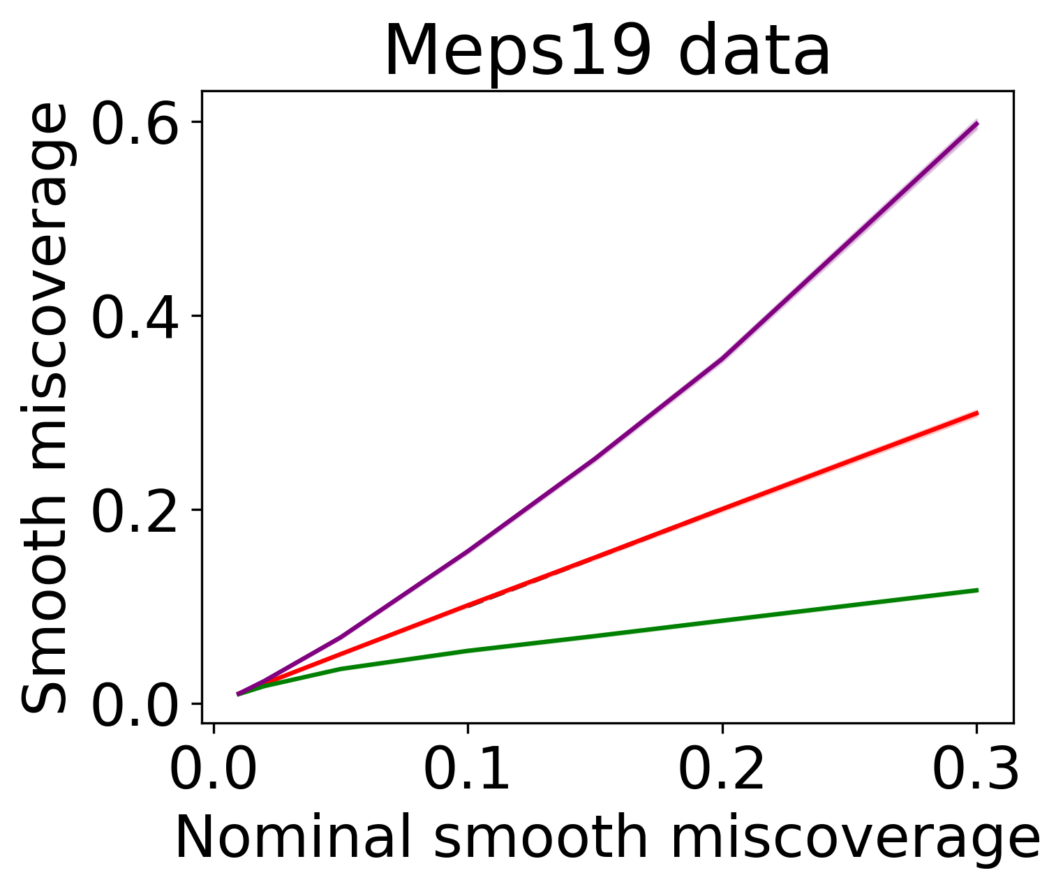
Figure 13: Smooth miscoverage rate achieved over noisy (red) and clean (green) test sets. The calibration scheme is applied using noisy annotations to control the smooth miscoverage level. Results are averaged over 10 random splits of the calibration and test sets.

4.6 Online learning

This section studies the effect of label noise on uncertainty quantification methods in an online learning setting, as formulated in Section 3.3.4. We experiment on a depth estimation task (Geiger et al., 2013), where the objective is to predict a depth map given a colored image. In other words, $X\in\mathbb{R}^{W\times H\times 3}$ is an input RGB image of size $W\times H$ and $Y\in\mathbb{R}^{W\times H}$ is its corresponding depth map. We consider the original depth values given in this data as ground truth and artificially corrupt them according to the additive noise model defined in (10) to produce noisy labels. Specifically, we add to each depth pixel an independent random noise drawn from a normal distribution with 0 mean and 0.7 variance. Here, the depth uncertainty of the $i,j$ pixel is represented by a prediction interval $C^{i,j}(X)\subseteq\mathbb{R}$. Ideally, the estimated intervals should contain the correct depth values at a pre-specified level $1-\alpha$. In this high-dimensional setting, this requirement is formalized as controlling the image miscoverage loss, defined as:

$$L^{\text{im}}(Y,C(X))=\frac{1}{WH}\sum_{i=1}^{W}{\sum_{j=1}^{H}{1\{Y^{i,j}\notin C^{i,j}(X)\}}}.$$ (35)

In words, the image miscoverage loss measures the proportion of depth values that were not covered in a given image. For this purpose, we employ the calibration scheme Rolling RC (Feldman et al., 2022), which constructs uncertainty sets in an online setting with a valid risk guarantee in the sense of (29). We follow the experimental protocol outlined in (Feldman et al., 2022, Section 4.2) and apply Rolling RC with an exponential stretching to control the image miscoverage loss at different levels on the observed, noisy, labels. We use LeReS (Yin et al., 2021) as a base model, which was pre-trained on a clean training set that corresponds to timestamps 1,…,6000. We continue training it and updating the calibration scheme in an online fashion on the following 2000 timestamps. We consider these samples, indexed by 6001 to 8000, as a validation set and use it to choose the calibration’s hyperparameters, as explained in (Feldman et al., 2022, Section 4.2). Finally, we continue the online procedure on the test samples whose indexes correspond to 8001 to 1000, and measure the performance on the clean and noisy versions of this test set. Figure 14 displays the risk achieved by this technique over the clean and corrupted labels. This figure indicates that Rolling RC attain valid image miscoverage over the unknown noiseless labels. This is not a surprise, as it is supported by Proposition A8 which guarantees conservative image miscoverage under label noise in an offline setting, and Proposition 3.5 which states that the former result applies to an online learning setting as well.

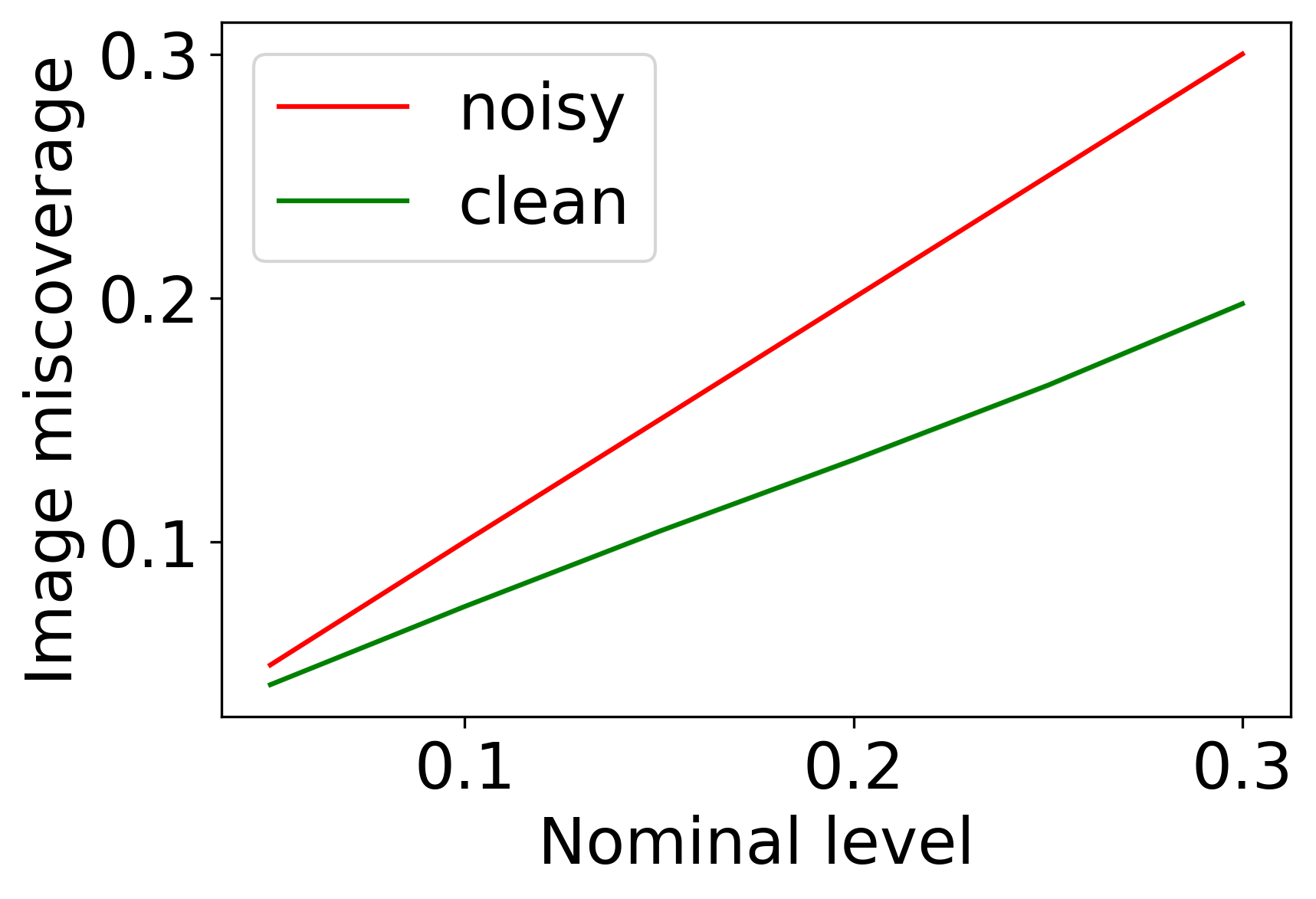
Figure 14: Image miscoverage achieved by Rolling RC. Results are averaged over 10 random trials.

5 Discussion

Our work raises many new questions. First, one can try and define a score function that is more robust to label noise, continuing the line of Gendler et al. (2021); Frénay and Verleysen (2013); Cheng et al. (2022). Second, an important remaining question is how to achieve exact risk control on the clean labels using minimal information about the noise model. Lastly, it would be interesting to analyze the robustness of alternative conformal methods such as cross-conformal and jackknife+ (Vovk, 2015; Barber et al., 2021) that do not require data-splitting.

Acknowledgments and Disclosure of Funding

Y.R., A.G., B.E., and S.F. were supported by the ISRAEL SCIENCE FOUNDATION (grant No. 729/21). Y.R. thanks the Career Advancement Fellowship, Technion, for providing research support. A.N.A. was supported by the National Science Foundation Graduate Research Fellowship Program under Grant No. DGE 1752814. S.F. thanks Aviv Adar, Idan Aviv, Ofer Bear, Tsvi Bekker, Yoav Bourla, Yotam Gilad, Dor Sirton, and Lia Tabib for annotating the MS COCO dataset.

Appendix A1 Mathematical proofs

Theorem 2.1.

Our assumption states that

$$\mathbb{P}(\tilde{s}_{\rm test}\leq t)\leq\mathbb{P}(s_{\rm test}\leq t).$$ (A1)

Note that the probability is only taken over $\tilde{s}_{\rm test}$. Since $\hat{q}_{\rm noisy}$ is constant (measurable) with respect to this probability, we have that, for any $\alpha\in(0,1)$,

$$\mathbb{P}(s_{\rm test}\leq\hat{q}_{\rm noisy})\geq\mathbb{P}(\tilde{s}_{\rm test}\leq\hat{q}_{\rm noisy})\geq 1-\alpha.$$ (A2)

This implies that $Y_{\rm test}\in\widehat{\mathcal{C}}_{\rm noisy}(X_{\rm test})$ with probability at least $1-\alpha$, completing the proof of the lower bound.

Regarding the upper bound, by the same argument,

$$\mathbb{P}(s_{\rm test}\leq\hat{q}_{\rm noisy})\leq\mathbb{P}(\tilde{s}_{\rm test}\leq\hat{q}_{\rm noisy})+u\leq 1-\alpha+\frac{1}{n+1}+u.$$ (A3)

∎

A1.1 General classification result

We commence by providing an extension to Proposition 2.2 and proving it.

Theorem A1.

Suppose that $\widehat{\mathcal{C}}_{\rm noisy}(x)$ constructs prediction sets that contain the most likely labels, i.e., $\forall x\in\mathcal{X},i\in\widehat{\mathcal{C}}_{\rm noisy}(x),j\notin\widehat{\mathcal{C}}_{\rm noisy}(x):\mathbb{P}(\tilde{Y}=i\mid X=x)\geq\mathbb{P}(\tilde{Y}=j\mid X=x)$. Further suppose that for all $x\in\mathcal{X}$:

1. $\forall m\in\{1,...,K\}:\sum_{i=1}^{m}{\left(\mathbb{P}(Y=o(x)_{i}\mid X=x)-\mathbb{P}(\tilde{Y}=o(x)_{i}\mid X=x)\right)}\geq 0.$

2. $\forall i,j\in\{1,..,K\}:\mathbb{P}(Y=i\mid X=x)\leq\mathbb{P}(Y=j\mid X=x)\iff\mathbb{P}(\tilde{Y}=i\mid X=x)\leq\mathbb{P}(\tilde{Y}=j\mid X=x).$

Above, $o(x)$ is a vector of length $K$ that contains the labels $j\in\{1,...,K\}$ ordered by their signal $\mathbb{P}(Y=j\mid X=x)$. The $i$-th element of $o(x)$, denoted by $o(x)_{i}$, is the label with the $i$-th maximal signal. If (1) and (2) hold, then the coverage rate achieved over the clean labels is bounded by:

$$\beta\leq\mathbb{P}(Y\in\widehat{\mathcal{C}}_{\rm noisy}(x)\mid X=x)\leq\beta+\frac{1}{2}\sum_{i=1}^{K}{|\mathbb{P}(\tilde{Y}=i\mid X=x)-\mathbb{P}({Y}=i\mid X=x)|},$$ (A4)

where $\beta:=\mathbb{P}(\tilde{Y}\in\widehat{\mathcal{C}}_{\rm noisy}(x)\mid X=x)$.

Proof.

First, for ease of notation, we omit the conditioning on $x$. Second, without loss of generality, we suppose that the labels are ranked from the most likely to the least likely, i.e., $\mathbb{P}(Y=i)\geq\mathbb{P}(Y=i+1)$. Since the prediction set contains the most likely labels, there exists some $1\leq m\leq K$ such that the prediction set is $C=\{1,2,...,m\}$. Notice that if $C=\emptyset$ the proposition is trivially satisfied.

We begin by proving the following lower bound $\mathbb{P}({Y}\in C)\geq\beta:=\mathbb{P}(\tilde{Y}\in C)$. Denote: $\delta_{i}:=\mathbb{P}(Y=i)-\mathbb{P}(\tilde{Y}=i)$. Since $\sum_{i=1}^{m}{\delta_{i}}\geq 0$ we get that:

$$\begin{split}\mathbb{P}(Y\in C)=\sum_{i=1}^{m}{\mathbb{P}(Y=i)}=\sum_{i=1}^{m}{\mathbb{P}(\tilde{Y}=i)}+\sum_{i=1}^{m}{\delta_{i}}\geq\sum_{i=1}^{m}{\mathbb{P}(\tilde{Y}=i)}+0=\mathbb{P}(\tilde{Y}\in C)=\beta.\end{split}$$ (A5)

We now turn to prove the upper bound. Denote by $1\leq g\in\mathbb{N}$ the index with the maximal $\sum_{i=1}^{g}{\delta_{i}}$.

$$\begin{split}\sum_{i=1}^{m}{\delta_{i}}\leq\sum_{i=1}^{g}{\delta_{i}}=\frac{1}{2}\left(\sum_{i=1}^{g}{\delta_{i}}+\sum_{i=1}^{g}{\delta_{i}}\right)=\frac{1}{2}\left(\sum_{i=1}^{g}{\delta_{i}}+\sum_{i=g+1}^{K}{-\delta_{i}}\right)=\frac{1}{2}\sum_{i=1}^{K}{|\delta_{i}|}=\frac{1}{2}\sum_{i=1}^{K}{|\mathbb{P}(\tilde{Y}=i)-\mathbb{P}({Y}=i)|}.\end{split}$$ (A6)

This gives us:

$$\mathbb{P}(Y\in C)=\mathbb{P}(\tilde{Y}\in C)+\sum_{i=1}^{m}{\delta_{i}}\leq\mathbb{P}(\tilde{Y}\in C)+\frac{1}{2}\sum_{i=1}^{K}{|\mathbb{P}(\tilde{Y}=i)-\mathbb{P}({Y}=i)|}.$$ (A7)

And this concludes the proof.

∎

We now turn to prove Proposition 2.2 using Theorem A1.

Proof.

We only need to show $\sum_{i=1}^{m}{\left(\mathbb{P}(Y=i)-\mathbb{P}(\tilde{Y}=i)\right)}\geq 0$ for all $m\in\{1,...,K\}$ and the results follow directly from Theorem A1. We follow the notations in the proof of Theorem A1. First, we observe that under the assumed noise model:

$$\mathbb{P}(Y=i)\geq\frac{1}{K}\iff\mathbb{P}(Y=i)\geq\mathbb{P}(\tilde{Y}=i)\iff\delta_{i}\geq 0.$$ (A8)

Denote by $1\leq g\in\mathbb{N}$ the largest index for which $\mathbb{P}(Y=g)\geq\frac{1}{K}$. It follows that:

$$\forall i\in\{1,...,K\}:i\leq g\iff\delta_{i}\geq 0.$$ (A9)

If $m\leq g$ then all summands in $\sum_{i=1}^{m}{\delta_{i}}$ are positive since $\delta_{i}\geq 0$ for every $i\leq m\leq g$. Thus, $\sum_{i=1}^{m}{\delta_{i}}\geq 0$ as required. Otherwise,

$$\sum_{i=1}^{m}{\delta_{i}}=\sum_{i=1}^{g}{\delta_{i}}+\sum_{i=g+1}^{m}{\delta_{i}}\underset{i>g\iff\delta_{i}\leq 0}{\geq}\sum_{i=1}^{g}{\delta_{i}}+\sum_{i=g+1}^{K}{\delta_{i}}=\sum_{i=1}^{K}{\delta_{i}}=0$$ (A10)

∎

Finally, we turn to prove Corollary 2.

Proof.

We follow the notations and assumptions in Theorem A1. We only need to show that $\frac{1}{2}\sum_{i=1}^{K}{|\delta_{i}|}\leq\varepsilon\frac{K-1}{K}$ and the results will follow directly from Theorem A1.

In the random flip setting, $|\delta_{i}|=\left|\mathbb{P}({Y}=i)\varepsilon-\frac{\varepsilon}{K}\right|=\varepsilon\left|\mathbb{P}({Y}=i)-\frac{1}{K}\right|$. Therefore:

$$\begin{split}\frac{1}{2}\sum_{i=1}^{K}{|\delta_{i}|}&=\frac{1}{2}\sum_{i=1}^{K}{\varepsilon\left|\mathbb{P}({Y}=i)-\frac{1}{K}\right|}\\ &=\frac{1}{2}\varepsilon\left(\sum_{i=1}^{g}{\left|\mathbb{P}({Y}=i)-\frac{1}{K}\right|}+\sum_{i=g+1}^{K}{\left|\mathbb{P}({Y}=i)-\frac{1}{K}\right|}\right)\\ &=\frac{1}{2}\varepsilon\left(\sum_{i=1}^{g}{\left(\mathbb{P}({Y}=i)-\frac{1}{K}\right)}+\sum_{i=g+1}^{K}{\left(\frac{1}{K}-\mathbb{P}({Y}=i)\right)}\right)\\ &=\frac{1}{2}\varepsilon\left(\sum_{i=1}^{g}{\mathbb{P}({Y}=i)}-\sum_{i=1}^{g}{\frac{1}{K}}+\sum_{i=g+1}^{K}{\frac{1}{K}}-\sum_{i=g+1}^{K}{\mathbb{P}({Y}=i)}\right)\\ &\leq\frac{1}{2}\varepsilon\left(1-\frac{g}{K}+\frac{K-g}{K}-0\right)\\ &\leq\frac{1}{2}\varepsilon\left(\frac{K-g}{K}+\frac{K-g}{K}\right)\\ &\leq\varepsilon\frac{K-g}{K}\\ &\leq\varepsilon\frac{K-1}{K}.\end{split}$$ (A11)

Thus, we get:

$$\mathbb{P}(\tilde{Y}\in C)\leq\mathbb{P}(Y\in C)\leq\mathbb{P}(\tilde{Y}\in C)+\frac{1}{2}\sum_{i=1}^{K}{|\mathbb{P}(\tilde{Y}=i)-\mathbb{P}({Y}=i)|}\leq\mathbb{P}(\tilde{Y}\in C)+\varepsilon\frac{K-1}{K}.$$ (A12)

which concludes the proof. ∎

A1.2 Confusion matrix

The confusion matrix noise model is more realistic than the uniform flip. However, there exists a score function that causes conformal prediction to fail for any non-identity confusion matrix. We define the corruption model as follows: consider a matrix $T$ in which $(T)_{i,j}=\mathbb{P}(\tilde{Y}=j\mid Y=i)$.

$$g^{\rm confusion}(y)=\begin{cases}1&\text{w.p. }T_{1,y}\\ \ldots&\\ K&\text{w.p. }T_{K,y}.\end{cases}$$ (A13)

Example 1.

Let $\widehat{\mathcal{C}}_{\rm noisy}$ be constructed as in Recipe 1 with any score function $s$ and the corruption function $g^{\rm confusion}$. Then,

$$\mathbb{P}\left(Y_{\rm test}\in\widehat{\mathcal{C}}_{\rm noisy}(X_{\rm test})\right)\geq 1-\alpha.$$ (A14)

if and only if for all classes $j\in\{1,\ldots,K\}$,

$$\sum\limits_{j^{\prime}=1}^{K}\mathbb{P}(\tilde{Y}=j^{\prime}\mid Y=j)\mathbb{P}(\tilde{s}\leq t\mid\tilde{Y}=j^{\prime})\geq\mathbb{P}(s\leq t\mid Y=j).$$ (A15)

The proof is below. In words, the necessary and sufficient condition is for the noise distribution/confusion matrix $\mathbb{P}(\tilde{Y}=j^{\prime}\mid Y=j)$ to place sufficient mass on those classes $j^{\prime}$ whose quantiles which are larger than $\mathbb{P}(s\leq t\mid Y=j)$. However, without assumptions on the model and score, the conditional probabilities are unknown, so it is impossible to say which noise distributions will preserve coverage.

Proof.

By law of total probability, $\mathbb{P}(s\leq t)=\mathbb{E}\left[\mathbb{P}(s\leq t\mid Y=j)\right]=\sum_{j=1}^{K}w_{j}\mathbb{P}(s\leq t\mid Y=j)$. But under the noisy model, we have instead that

$$\mathbb{P}(\tilde{s}\leq t)=\mathbb{E}\left[\mathbb{P}(\tilde{s}\leq t\mid\tilde{Y}=j^{\prime})\right]=\sum\limits_{j=1}^{K}\sum\limits_{j^{\prime}=1}^{K}w_{j}\mathbb{P}(\tilde{Y}=j^{\prime}\mid Y=j)\mathbb{P}(\tilde{s}\leq t\mid\tilde{Y}=j^{\prime}).$$ (A16)

We can write

$$\mathbb{P}(s\leq t)-\mathbb{P}(\tilde{s}\leq t)=\sum\limits_{j=1}^{K}\sum\limits_{j^{\prime}=1}^{K}w_{j}\mathbb{P}(\tilde{Y}=j^{\prime}\mid Y=j)\mathbb{P}(\tilde{s}\leq t\mid\tilde{Y}=j^{\prime})-\sum\limits_{j=1}^{K}w_{j}\mathbb{P}(s\leq t\mid Y=j).$$ (A17)

Combining the sums and factoring, the above display equals

$$\sum\limits_{j=1}^{K}w_{j}\left(\sum\limits_{j^{\prime}=1}^{K}\left(\mathbb{P}(\tilde{Y}=j^{\prime}\mid Y=j)\mathbb{P}(\tilde{s}\leq t\mid\tilde{Y}=j^{\prime})\right)-\mathbb{P}(s\leq t\mid Y=j)\right).$$ (A18)

We can factor this expression as

$$\sum\limits_{j=1}^{K}w_{j}\mathbb{P}(s\leq t\mid Y=j)\sum\limits_{j^{\prime}=1}^{K}\left(\mathbb{P}(\tilde{Y}=j^{\prime}\mid Y=j)\frac{\mathbb{P}(\tilde{s}\leq t\mid\tilde{Y}=j^{\prime})}{\mathbb{P}(s\leq t\mid Y=j)}-\frac{1}{K}\right).$$ (A19)

The stochastic dominance condition holds uniformly over all choices of base probabilities $w_{j}$ if and only if for all $j\in[K]$,

$$\sum\limits_{j^{\prime}=1}^{K}\mathbb{P}(\tilde{Y}=j^{\prime}\mid Y=j)\mathbb{P}(\tilde{s}\leq t\mid\tilde{Y}=j^{\prime})\geq\mathbb{P}(s\leq t\mid Y=j).$$ (A20)

∎

Notice that the left-hand side of the above display is a convex mixture of the quantiles $\mathbb{P}(\tilde{s}\leq t\mid\tilde{Y}=j^{\prime})$ for $j^{\prime}\in[K]$. Thus, the necessary and sufficient condition is for the noise distribution $\mathbb{P}(\tilde{Y}=j^{\prime}\mid Y=j)$ to place sufficient mass on those classes $j^{\prime}$ whose quantiles which are larger than $\mathbb{P}(s\leq t\mid Y=j)$. But of course, without assumptions on the model and score, the latter are unknown, so it is impossible to say which noise distributions will preserve coverage.

A1.3 General regression result

Theorem A2.

Suppose an additive noise model $g^{\rm add}$ with a noise that has mean 0. Denote the prediction interval as $C(x)=[a_{x},b_{x}]$. If for all $x\in\mathcal{X}$ density of $Y\mid X=x$ is peaked inside the interval:

1. $\forall\varepsilon\geq 0:f_{Y\mid X=x}(b_{x}+\varepsilon)\leq f_{Y\mid X=x}(b_{x}-\varepsilon).$

2. $\forall\varepsilon\geq 0:f_{Y\mid X=x}(a_{x}-\varepsilon)\leq f_{Y\mid X=x}(a_{x}+\varepsilon).$

then, we obtain valid conditional coverage:

$$\mathbb{P}(Y\in C(x)\mid X=x)\geq\mathbb{P}(\tilde{Y}\in C(x)\mid X=x).$$ (A21)

Proof.

For ease of notation, we omit the conditioning on $X=x$. In other words, we treat $Y$ as $Y\mid X=x$ for some $x\in\mathcal{X}$. We begin by showing $\mathbb{P}(\tilde{Y}\leq b)\geq\mathbb{P}(Y\leq b)$.

$$\begin{split}&\mathbb{P}(\tilde{Y}\leq b)\\ &=\mathbb{P}(Y+\varepsilon\leq b)\\ &=\mathbb{P}(Y+\varepsilon\leq b\mid\varepsilon\geq 0)\mathbb{P}(\varepsilon\geq 0)+\mathbb{P}(Y+\varepsilon\leq b\mid\varepsilon\leq 0)\mathbb{P}(\varepsilon\leq 0)\\ &=\frac{1}{2}\mathbb{P}(Y+\varepsilon\leq b\mid\varepsilon\geq 0)+\frac{1}{2}\mathbb{P}(Y+\varepsilon\leq b\mid\varepsilon\leq 0)\\ &=\frac{1}{2}\mathbb{P}(Y\leq b-\varepsilon\mid\varepsilon\geq 0)+\frac{1}{2}\mathbb{P}(Y\leq b+\varepsilon\mid\varepsilon\geq 0)\\ &=\frac{1}{2}\mathbb{E}_{\varepsilon\geq 0}\left[\mathbb{P}(Y\leq b-\varepsilon)+\mathbb{P}(Y\leq b+\varepsilon)\right]\\ &=\mathbb{P}(Y\leq b)+\frac{1}{2}\mathbb{E}_{\varepsilon\geq 0}\left[\mathbb{P}(Y\leq b-\varepsilon)-\mathbb{P}(Y\leq b)+\mathbb{P}(Y\leq b+\varepsilon)-\mathbb{P}(Y\leq b)\right]\\ &=\mathbb{P}(Y\leq b)+\frac{1}{2}\mathbb{E}_{\varepsilon\geq 0}\left[\mathbb{P}(Y\leq b+\varepsilon)-\mathbb{P}(Y\leq b)-(\mathbb{P}(Y\leq b)-\mathbb{P}(Y\leq b-\varepsilon))\right]\\ &=\mathbb{P}(Y\leq b)+\frac{1}{2}\mathbb{E}_{\varepsilon\geq 0}\left[\mathbb{P}(b\leq Y\leq b+\varepsilon)-\mathbb{P}(b-\varepsilon\leq Y\leq b)\right]\\ &\leq\mathbb{P}(Y\leq b)+\frac{1}{2}\mathbb{E}_{\varepsilon\geq 0}\left[0\right]\\ &=\mathbb{P}(Y\leq b).\end{split}$$ (A22)

The last inequality follows from the assumption that $\forall\varepsilon\geq 0:f_{Y}(b+\varepsilon)\leq f_{Y}(b-\varepsilon)$. The proof for $\mathbb{P}(\tilde{Y}\geq a)\leq\mathbb{P}(Y\geq a)$ is similar and hence omitted. We get that:

$$\begin{split}&\mathbb{P}(\tilde{Y}\in C(x))\\ &=\mathbb{P}(a\leq\tilde{Y}\leq b)\\ &=\mathbb{P}(\tilde{Y}\leq b)-\mathbb{P}(\tilde{Y}\geq a)\\ &\leq\mathbb{P}(Y\leq b)-\mathbb{P}(Y\geq a)\text{ (follows from the above)}\\ &=\mathbb{P}(a\leq Y\leq b)\\ &=\mathbb{P}(Y\in C(x)).\end{split}$$ (A23)

∎

We now turn to prove Proposition 2.1 using Theorem A2

Proof.

Since the density of $Y\mid X=x$ is symmetric and unimodal for all $x\in\mathcal{X}$ it is peaked inside any prediction interval that contains its median. Therefore, the prediction interval achieves valid conditional coverage:

$$\forall x\in\mathcal{X}:\mathbb{P}(\tilde{Y}\in C(x)\mid X=x)\geq\mathbb{P}(Y\in C(x)\mid X=x).$$ (A24)

By taking the expectation over $X\sim P_{X}$ we obtain valid marginal coverage. ∎

A1.4 General risk bound for regression tasks

Proof of Proposition 3.3.

For ease of notation, we omit the conditioning on $X=x$. In other words, we treat $Y$ as $Y\mid X=x$ for some $x\in\mathcal{X}$. Given a prediction set $\hat{C}(x)$, we consider the loss as a function of $Y$, where $\hat{C}(x)$ is fixed, and denote it by:

$$L(Y):=L(Y,\hat{C}(x)).$$ (A25)

We expand $L(Y+\varepsilon)$ using Taylor’s expansion:

$$\begin{split}L(Y+\varepsilon)&=L(Y)+\varepsilon L^{\prime}(Y)+\frac{1}{2}\varepsilon^{2}L^{\prime\prime}(\xi),\end{split}$$ (A26)

where $\xi$ is some real number between $Y$ and $Y+\varepsilon$.

$$\begin{split}\delta&:=L(\tilde{Y})-L(Y)\\ &=L(Y+\varepsilon)-L(Y)\\ &=\varepsilon L^{\prime}(Y)+\frac{1}{2}\varepsilon^{2}L^{\prime\prime}(\xi).\\ \end{split}$$ (A27)

We now develop each term separately. Since $\varepsilon\perp\!\!\!\perp Y$ it follows that $\varepsilon\perp\!\!\!\perp L^{\prime}(Y)$.

$$\begin{split}\mathbb{E}\left[\varepsilon L^{\prime}(Y)\right]=\mathbb{E}\left[\varepsilon\right]\mathbb{E}\left[L^{\prime}(Y)\right]=0\mathbb{E}\left[L^{\prime}(Y)\right]=0\end{split}$$ (A28)

Since $L^{\prime\prime}(y)$ is bounded by $q\leq L^{\prime\prime}(y)\leq Q$, we get the following:

$$\begin{split}\frac{1}{2}q\text{Var}\left[\varepsilon\right]=\frac{1}{2}q\mathbb{E}\left[\varepsilon^{2}\right]=\mathbb{E}\left[\frac{1}{2}\varepsilon^{2}q_{x}\right]\leq\mathbb{E}\left[\frac{1}{2}\varepsilon^{2}L^{\prime\prime}(\xi)\right]\leq\mathbb{E}\left[\frac{1}{2}\varepsilon^{2}Q_{x}\right]=\frac{1}{2}Q\mathbb{E}\left[\varepsilon^{2}\right]=\frac{1}{2}Q\text{Var}\left[\varepsilon\right]\end{split}$$ (A29)

We get that:

$$\begin{split}\mathbb{E}[\delta]=\mathbb{E}\left[\varepsilon L^{\prime}(Y)+\frac{1}{2}\varepsilon^{2}L^{\prime\prime}(\xi)\right]=0+\mathbb{E}\left[\frac{1}{2}\varepsilon^{2}L^{\prime\prime}(\xi)\right].\end{split}$$ (A30)

Therefore:

$$\begin{split}&\frac{1}{2}q\text{Var}\left[\varepsilon\right]\leq\mathbb{E}[\delta]\leq\frac{1}{2}Q\text{Var}\left[\varepsilon\right].\\ &\Rightarrow\frac{1}{2}q\text{Var}\left[\varepsilon\right]\leq\mathbb{E}\left[L(\tilde{Y},\hat{C}(X))-L({Y},\hat{C}(X))\right]\leq\frac{1}{2}Q\text{Var}\left[\varepsilon\right].\end{split}$$ (A31)

We now turn to consider the conditioning on $X=x$ and obtain marginalized bounds by taking the expectation over all $X$:

$$\begin{split}\alpha-\frac{1}{2}Q\text{Var}\left[\varepsilon\right]\leq\mathbb{E}\left[L({Y},\hat{C}(X))\right]\leq\alpha-\frac{1}{2}q\text{Var}\left[\varepsilon\right]\end{split}$$ (A32)

where $\alpha:=\mathbb{E}\left[L({Y},\hat{C}(X))\right]$, $q:=\mathbb{E}_{X}[q_{X}]$, and $Q:=\mathbb{E}_{X}[Q_{X}]$. Additionally, if $L(y,C(x))$ is convex for all $x\in{\mathcal{X}}$, then $q_{x}\geq 0$, and we get conservative coverage:

$$\begin{split}\mathbb{E}\left[L({Y},\hat{C}(X))\right]\leq\mathbb{E}\left[L(\tilde{Y},\hat{C}(X))\right]=\alpha.\end{split}$$ (A33)

∎

A1.5 Deriving a miscoverage bound from the general risk bound in regression tasks

In this section we prove Proposition 3.4 and show how to obtain tight coverage bounds. First, we define a parameterized smoothed miscoverage loss:

$$L^{sm}_{d,c}(y,[a,b])=\frac{2}{1+e^{-d\left(\left(2\frac{y-a}{b-a}-1\right)^{2}\right)^{c}}}.$$ (A34)

Above, $c,d\in\mathbb{R}$ are parameters that affect the loss function. We first connect between the smooth miscoverage and the standard miscoverage functions:

$$\begin{split}L(y,[a,b])=\mathbbm{1}\{L^{sm}_{d,c}(y,[a,b])\geq h\}.\end{split}$$ (A35)

We now invert the above equation to find $h$:

$$\begin{split}h&=L^{sm}_{d,c}\left(\min_{L(y,[a,b])=0}{y},[a,b]\right)\\ &=L^{sm}_{d,c}\left(\max_{L(y,[a,b])=0}{y},[a,b]\right)\\ &=L^{sm}_{d,c}\left(a,[a,b]\right)\\ &=L^{sm}_{d,c}\left(b,[a,b]\right)\\ &=\frac{2}{1+e^{-d\left(\left(2\frac{a-a}{b-a}-1\right)^{2}\right)^{c}}}\\ &=\frac{2}{1+e^{-d\left(\left(-1\right)^{2}\right)^{c}}}\\ &=\frac{2}{1+e^{-d}}.\end{split}$$ (A36)

Therefore, $h(d)$ is a function that depends only on $d$. We now denote the second derivative of the smoothed loss by:

$$\begin{split}q_{x}(c,d)=\min_{y}{\frac{\partial^{2}}{\partial y^{2}}L^{sm}_{c,d}(y,C(x))}.\end{split}$$ (A37)

Importantly, $q_{x}(c,d)$ can be empirically computed by sweeping over all $y\in\mathbb{R}$ and computing the second derivative of $L^{sm}_{c,d}$ for each of them.

We obtain an upper bound for the miscoverage of $C(x)$ by applying Markov’s inequality using A35:

$$\begin{split}\mathbb{P}(Y\notin C(X)\mid X=x)=\mathbb{P}(L^{sm}_{d,c}(Y,C(X))\geq h(d)\mid X=x)\leq\frac{\mathbb{E}\left[L^{sm}_{c,d}({Y},{C}(X))\mid X=x\right]}{h(d)}.\end{split}$$ (A38)

Next, we employ smoothed miscoverage upper bound provided by Proposition 3.4:

$$\begin{split}\mathbb{E}\left[L^{sm}_{c,d}({Y},{C}(X))\mid X=x\right]\leq\mathbb{E}\left[L^{sm}_{c,d}(\tilde{Y},{C}(X))\mid X=x\right]-\frac{1}{2}q_{x}(c,d)\text{Var}\left[\varepsilon\right]\end{split}$$ (A39)

Finally, we combine A38 and A39 and derive the following miscoverage bound:

$$\begin{split}\mathbb{P}(Y\notin C(X)\mid X=x)\leq\frac{\mathbb{E}\left[L^{sm}_{c,d}(\tilde{Y},{C}(X))\mid X=x\right]-\frac{1}{2}q_{x}(c,d)\text{Var}\left[\varepsilon\right]}{h(d)},\end{split}$$ (A40)

which can be restated to:

$$\begin{split}\mathbb{P}(Y\in C(X)\mid X=x)\geq 1-\frac{\mathbb{E}\left[L^{sm}_{c,d}(\tilde{Y},{C}(X))\mid X=x\right]-\frac{1}{2}q_{x}(c,d)\text{Var}\left[\varepsilon\right]}{h(d)}.\end{split}$$ (A41)

Finally, we take the expectation over all $X$ to obtain marginal coverage bound:

$$\begin{split}\mathbb{P}(Y\in C(X))\geq 1-\frac{\mathbb{E}\left[L^{sm}_{c,d}(\tilde{Y},{C}(X))\right]-\frac{1}{2}\mathbb{E}_{X}[q_{x}(c,d)]\text{Var}\left[\varepsilon\right]}{h(d)}.\end{split}$$ (A42)

Crucially, all variables in (A42) are empirically computable so the above lower bound can is known in practice. Additionally, the parameters $c,d$ can be tuned over a validation set to obtain tighter bounds.

A1.6 Deriving a miscoverage bound from the density’s smoothness

We say that the PDF of $Y\mid X=x$ is $K_{x}$ Lipschitz if

$$|f_{Y\mid X=x}(y+u)-f_{Y\mid X=x}(y)|\leq K_{x}u,$$ (A43)

where $f_{Y\mid X=x}$ is the PDF of $Y\mid X=x$ and $K_{x}\in\mathbb{R}$ is a constant that depends only on $x$.

Proposition A3.

Suppose that $C(x)$ is a prediction interval. Under the additive noise model $g^{\text{add}}$ from (10), if the PDF of $Y\mid X=x$ is $K_{x}$ Lipschitz then:

$$\mathbb{P}(Y\in C(X))\geq\mathbb{P}(\tilde{Y}\in C(X))-\mathbb{E}\left[|C(X)|K_{X}\right]\mathbb{E}\left[|Z|\right].$$ (A44)

Proof.

First, by the definition of the noise model we get that:

$$\begin{split}f_{\tilde{Y}\mid X=x}(y)&=\int_{-\infty}^{\infty}f_{Y\mid X=x}(y-z)f_{Z}(z)\,dz\\ &\leq\int_{-\infty}^{\infty}(f_{Y\mid X=x}(y)+K_{x}|z|)f_{Z}(z)\,dz\\ &=f_{Y\mid X=x}(y)\int_{-\infty}^{\infty}f_{Z}(z)\,dz+K_{x}\int_{-\infty}^{\infty}|z|f_{Z}(z)\,dz\\ &=f_{Y\mid X=x}(y)+K_{x}\mathbb{E}[|Z|].\end{split}$$ (A45)

Therefore:

$$\begin{split}\mathbb{P}(Y\in C(X)\mid X=x)&=\int_{y\in C(x)}f_{Y\mid X=x}(y)\,dy\\ &\geq\int_{y\in C(x)}(f_{\tilde{Y}\mid X=x}(y)-K_{x}\mathbb{E}[|Z|])\,dy\\ &=\mathbb{P}(\tilde{Y}\in C(X)\mid X=x)-|C(x)|K_{x}\mathbb{E}[|Z|].\end{split}$$ (A46)

We marginalize the above to obtain the marginal coverage bound:

$$\begin{split}\mathbb{P}(Y\in C(X))=\mathbb{P}(\tilde{Y}\in C(X))-\mathbb{E}[|C(X)|K_{X}]\mathbb{E}[|Z|].\end{split}$$ (A47)

∎

A1.7 Distribution-free results

Proof of Proposition 2.3.

For convenience, assume the existence of probability density functions $\tilde{p}$ and $p$ for $\tilde{Y}$ and $Y$ respectively (these can be taken to be probability mass functions if $\mathcal{Y}$ is discrete). Also define the multiset of $Y$ values $E=\{Y_{1},...,Y_{n}\}$ and the corresponding multiset of $\tilde{Y}$ values $\tilde{E}$. Take the set

$$\mathcal{A}=\{y:\tilde{p}(y)>p(y)\}.$$ (A48)

Since $Y\overset{d}{\neq}\tilde{Y}$, we know that the set $\mathcal{A}$ is nonempty and $\mathbb{P}(\tilde{Y}\in\mathcal{A})=\delta_{1}>\mathbb{P}(Y\in\mathcal{A})=\delta_{2}\geq 0$. The adversarial choice of score function will be $s(x,y)=\mathbbm{1}\left\{y\in\mathcal{A}^{c}\right\}$; it puts high mass wherever the ground truth label is more likely than the noisy label. The crux of the argument is that this design makes the quantile smaller when it is computed on the noisy data than when it is computed on clean data, as we next show.

Begin by noticing that, because $s(x,y)$ is binary, $\hat{q}_{\rm clean}$ is also binary, and therefore $\hat{q}_{\rm clean}>t\Longleftrightarrow\hat{q}_{\rm clean}=1$. Furthermore, $\hat{q}_{\rm clean}=1$ if and only if $|E\cap\mathcal{A}|\big{|}<\lceil(n+1)(1-\alpha)\rceil$. Thus, these events are the same, and for any $t\in(0,1]$,

$$\mathbb{P}\left(\hat{q}_{\rm clean}\geq t\right)=\mathbb{P}\Big{(}\big{|}E\cap\mathcal{A}\big{|}<\lceil(n+1)(1-\alpha)\rceil\Big{)}.$$ (A49)

By the definition of $\mathcal{A}$, we have that $\mathbb{P}\Big{(}\big{|}E\cap\mathcal{A}\big{|}<\lceil(n+1)(1-\alpha)\rceil\Big{)}>\mathbb{P}\Big{(}\big{|}\tilde{E}\cap\mathcal{A}\big{|}<\lceil(n+1)(1-\alpha)\rceil\Big{)}$. Chaining the inequalities, we get

$$\mathbb{P}\left(\hat{q}_{\rm clean}\geq t\right)>\mathbb{P}\Big{(}\big{|}\tilde{E}\cap\mathcal{A}\big{|}<\lceil(n+1)(1-\alpha)\rceil\Big{)}=\mathbb{P}\left(\hat{q}\geq t\right).$$ (A50)

Since $s_{n+1}$ is measurable with respect to $E$ and $\tilde{E}$, we can plug it in for $t$, yielding the conclusion. ∎

Remark A4.

In the above argument, if one further assumes continuity of the (ground truth) score function and $\mathbb{P}(\tilde{Y}\in\mathcal{A})=\mathbb{P}(Y\in\mathcal{A})+\rho$ for

$$\rho=\inf\Big{\{}\rho^{\prime}>0\;:\; \mathrm{BinomCDF}(n,\delta_{1},\lceil(n+1)(1-\alpha)\rceil-1)+\frac{1}{n}<$$ (A51)

$$\mathrm{BinomCDF}(n,\delta_{2}+\rho^{\prime},\lceil(n+1)(1-\alpha)\rceil-1)\Big{\}},$$ (A52)

then

$$\mathbb{P}(s_{n+1}\leq\hat{q})<1-\alpha.$$ (A53)

In other words, the noise must have some sufficient magnitude in order to disrupt coverage.

Proof of Corollary 3.

This a consequence of the TV bound from Barber et al. (2022) with weights identically equal to $1$. ∎

Unfortunately, getting such a TV bound requires a case by case analysis. It’s not even straightforward to get a TV bound under strong Gaussian assumptions.

Proposition A1.1 (No general TV bound).

Assume $Y\sim\mathcal{N}(0,\tau^{2})$ and $\tilde{Y}=y+Z$, where $Z\sim\mathcal{N}(0,\sigma^{2})$. Then $D_{\rm TV}(Y,\tilde{Y})\overset{\tau\to 0}{\to}1$.

Proof.

$$\mathrm{TV}(\mathcal{N}(0,\tau^{2}),\mathcal{N}(0,\tau^{2}+\sigma^{2}))=\int\limits_{-\infty}^{\infty}\Big{|}e^{-x^{2}/\tau^{2}}-e^{-x^{2}/(\tau^{2}+\sigma^{2})}\Big{|}dx\overset{\tau\to 0}{\to}1.$$ (A54)

∎

A1.8 False-negative rate

In this section, we prove all FNR robustness propositions. Here, we suppose that the response $Y\in[0,1]^{n}$ is a binary vector of size $n\in\mathbb{N}$, where $Y_{i}=1$ indicates that the $i$-th label is present. We further suppose a vector-flip noise model from (21), where $\varepsilon$ is a binary random vector of size $n$ as well. These notations apply for segmentation tasks as well, by flattening the response matrix into a vector. The prediction set $C(X)\subseteq\{1,...,n\}$ contains a subset of the labels. We begin by providing additional theoretical results and then turn to the proofs.

A1.8.1 Additional theoretical results

Proposition A1.2.

Let $\widehat{\mathcal{C}}_{\rm noisy}(X_{\rm test})$ be a prediction set that controls the FNR risk of the noisy labels at level $\alpha$. Suppose that

1. The prediction set contains the most likely labels in the sense that for all $x\in\mathcal{X}$, $k\in\widehat{\mathcal{C}}_{\rm noisy}(x)$, $i\notin\widehat{\mathcal{C}}_{\rm noisy}(x)$ and $m\in\mathbb{N}$:

   $$\mathbb{P}\left(\tilde{Y}_{k}=1\middle|\sum_{j\neq i,k}{\tilde{Y}_{j}}=m,X=x\right)\geq\mathbb{P}\left(\tilde{Y}_{k}=1\middle|\sum_{j\neq i,k}{\tilde{Y}_{j}}=m,X=x\right).$$ (A55)

2. For a given input $X=x$, the noise level of all response elements is the same, i.e., for all $i\neq j\in\{1\dots K\}$: $\mathbb{P}(\epsilon_{i}=1\mid X=x)=\mathbb{P}(\epsilon_{j}=1\mid X=x)$.

3. The noise is independent of $Y\mid X=x$ in the sense that $\epsilon\perp\!\!\!\perp Y\mid X=x$ for all $x\in\mathcal{X}$.

4. The noises of different labels are independent of each other given $X$, i.e., $\epsilon_{i}\perp\!\!\!\perp\epsilon_{j}\mid X=x$ for all $i\neq j\in\{1,\dots K\}$ and $x\in\mathcal{X}$.

Then

$$\mathbb{E}\left[L^{\rm FNR}\left(Y_{\rm test},\widehat{\mathcal{C}}_{\rm noisy}(X_{\rm test})\right)\right]\leq\alpha.$$ (A56)

A1.8.2 General derivations

In this section, we formulate and prove a general lemma that is used to prove label-noise robustness with the false-negative rate loss.

Lemma A5.

Suppose that $x\in\mathcal{X}$ is an input variable and $C(x)$ is a prediction set. Denote by $\beta_{i}$ the noise level at the $i$-th element: $\beta_{i}:=\mathbb{P}(\varepsilon_{i}=1\mid X=x)$. We define:

$$e_{k,i}(y):=\beta_{i}{{y_{k}\mathbb{E}\left[\frac{1}{\sum_{j=1}^{n}{\tilde{Y}_{j}}}\middle|\varepsilon_{i}=1,Y=y\right]}}.$$ (A57)

If for all $k\in C(x)$ and $i\notin C(x)$:

$$\mathbb{E}\left[\frac{e_{k,i}(Y)-e_{i,k}(Y)}{\sum_{j=1}^{n}Y_{j}}\middle|X=x\right]\geq 0$$ (A58)

Then $C(x)$ achieves conservative conditional risk:

$$\mathbb{E}\left[L^{\text{FNR}}(Y,C(X))\mid X=x\right]\leq\mathbb{E}\left[L^{\text{FNR}}(\tilde{Y},C(X))\mid X=x\right].$$ (A59)

Furthermore, $C(X)$ achieves valid marginal risk:

$$\mathbb{E}\left[L^{\text{FNR}}(Y,C(X))\right]\leq\mathbb{E}\left[L^{\text{FNR}}(\tilde{Y},C(X))\right].$$ (A60)

Proof.

For ease of notation, we omit the conditioning on $X=x$. That, we take some $x\in\mathcal{X}$ and treat $Y$ as $Y\mid X=x$. We also denote the prediction set as $C=C(x)$. Denote:

$$\delta:=L^{\text{FNR}}(\tilde{Y},C)-L^{\text{FNR}}({Y},C).$$ (A61)

Our goal is to show that:

$$\mathbb{E}\left[\delta\right]\geq 0.$$ (A62)

If $C=\emptyset$ or $C=\{1,...,n\}$ then the proposition is trivially satisfied. Therefore, for the rest of this proof, we assume that $C\neq\emptyset,\{1,...,n\}$. We begin by developing $\delta$ as follows.

$$\begin{split}\delta&=L^{\text{FNR}}(\tilde{Y},C)-L^{\text{FNR}}({Y},C)\\ &=\frac{\sum_{j\in C}{Y_{j}}}{\sum_{j}Y_{j}}-\frac{\sum_{j\in C}{[Y_{j}-2\varepsilon_{j}Y_{j}+\varepsilon_{j}]}}{\sum_{j}{Y_{j}-2\varepsilon_{j}Y_{j}+\varepsilon_{j}}}\\ &=\frac{\sum_{i}\sum_{j\in C}{Y_{j}[Y_{i}-2\varepsilon_{i}Y_{i}+\varepsilon_{i}]}-\sum_{i}\sum_{j\in C}{Y_{i}[Y_{j}-2\varepsilon_{j}Y_{j}+\varepsilon_{j}]}}{(\sum_{j}Y_{j})(\sum_{j}{Y_{j}-2\varepsilon_{j}Y_{j}+\varepsilon_{j}})}\\ &=\frac{\sum_{i}\sum_{j\in C}{Y_{j}Y_{i}-2Y_{j}\varepsilon_{i}Y_{i}+Y_{j}\varepsilon_{i}}-\sum_{i}\sum_{j\in C}{Y_{i}Y_{j}-2Y_{i}\varepsilon_{j}Y_{j}+Y_{i}\varepsilon_{j}}}{(\sum_{j}Y_{j})(\sum_{j}{Y_{j}-2\varepsilon_{j}Y_{j}+\varepsilon_{j}})}\\ &=\frac{\sum_{i}\sum_{j\in C}{Y_{j}Y_{i}-2Y_{j}\varepsilon_{i}Y_{i}+Y_{j}\varepsilon_{i}-[Y_{i}Y_{j}-2Y_{i}\varepsilon_{j}Y_{j}+Y_{i}\varepsilon_{j}]}}{(\sum_{j}Y_{j})(\sum_{j}{Y_{j}-2\varepsilon_{j}Y_{j}+\varepsilon_{j}})}\\ &=\frac{\sum_{i}\sum_{j\in C}{Y_{j}\varepsilon_{i}-Y_{i}\varepsilon_{j}}}{(\sum_{j}Y_{j})(\sum_{j}{Y_{j}-2\varepsilon_{j}Y_{j}+\varepsilon_{j}})}\\ &=\frac{(\sum_{i}{\varepsilon_{i}})(\sum_{j\in C}{Y_{j})}-(\sum_{i}{Y_{i}})(\sum_{j\in C}{\varepsilon_{j})}}{(\sum_{j}Y_{j})(\sum_{j}{Y_{j}-2\varepsilon_{j}Y_{j}+\varepsilon_{j}})}.\\ \end{split}$$ (A63)

Without loss of generality, we assume that $C=\{1,...,p\}$. We now compute the expectation of each term separately.

$$\begin{split}&\mathbb{E}\left[\frac{(\sum_{i}{\varepsilon_{i}})(\sum_{k=1}^{p}{Y_{k}})}{(\sum_{j}Y_{j})(\sum_{j}{Y_{j}-2\varepsilon_{j}Y_{j}+\varepsilon_{j}})}\middle|Y=y\right]\\ &=\sum_{i}{\mathbb{E}\left[\frac{{\varepsilon_{i}}(\sum_{k=1}^{p}{Y_{k}})}{(\sum_{j}Y_{j})(\sum_{j}{Y_{j}-2\varepsilon_{j}Y_{j}+\varepsilon_{j}})}\middle|Y=y\right]}\\ &=\sum_{i}{\frac{(\sum_{k=1}^{p}{y_{k}})}{\sum_{j}y_{j}}\mathbb{E}\left[\frac{\varepsilon_{i}}{\sum_{j}{Y_{j}-2\varepsilon_{j}Y_{j}+\varepsilon_{j}}}\middle|Y=y\right]}\\ &=\sum_{i}{\frac{(\sum_{k=1}^{p}{y_{k}})}{\sum_{j}y_{j}}\mathbb{E}\left[\frac{\varepsilon_{i}}{\sum_{j}{Y_{j}-2\varepsilon_{j}Y_{j}+\varepsilon_{j}}}\middle|\varepsilon_{i}=1,Y=y\right]\mathbb{P}(\varepsilon_{i}=1)}\\ &=\frac{1}{\sum_{j}y_{j}}\sum_{i}{\beta_{i}\left(\sum_{k=1}^{p}{y_{k}}\right)\mathbb{E}\left[\frac{1}{(1-Y_{i})+\sum_{j\neq i}{Y_{j}-2\varepsilon_{j}Y_{j}+\varepsilon_{j}}}\middle|\varepsilon_{i}=1,Y=y\right]}\\ &=\frac{1}{\sum_{j}y_{j}}\sum_{i}{{\sum_{k=1}^{p}\beta_{i}y_{k}\mathbb{E}\left[\frac{1}{(1-Y_{i})+\sum_{j\neq i}{Y_{j}-2\varepsilon_{j}Y_{j}+\varepsilon_{j}}}\middle|\varepsilon_{i}=1,Y=y\right]}}\\ \end{split}$$ (A64)

$$\begin{split}&\mathbb{E}\left[\frac{(\sum_{i}{Y_{i}})(\sum_{k=1}^{p}\varepsilon_{k})}{(\sum_{j}Y_{j})(\sum_{j}{Y_{j}-2\varepsilon_{j}Y_{j}+\varepsilon_{j}})}\middle|Y=y\right]\\ &=\sum_{i}{\mathbb{E}\left[\frac{{Y_{i}}(\sum_{k=1}^{p}\varepsilon_{k})}{(\sum_{j}Y_{j})(\sum_{j}{Y_{j}-2\varepsilon_{j}Y_{j}+\varepsilon_{j}})}\middle|Y=y\right]}\\ &=\sum_{i}{\frac{y_{i}}{\sum_{j}y_{j}}\mathbb{E}\left[\frac{(\sum_{k=1}^{p}\varepsilon_{k})}{\sum_{j}{Y_{j}-2\varepsilon_{j}Y_{j}+\varepsilon_{j}}}\middle|Y=y\right]}\\ &=\sum_{i}{\frac{y_{i}}{\sum_{j}y_{j}}\sum_{k=1}^{p}\mathbb{E}\left[\frac{\varepsilon_{k}}{\sum_{j}{Y_{j}-2\varepsilon_{j}Y_{j}+\varepsilon_{j}}}\middle|Y=y\right]}\\ &=\sum_{i}{\frac{y_{i}}{\sum_{j}y_{j}}\sum_{k=1}^{p}{\beta_{k}\mathbb{E}\left[\frac{\varepsilon_{k}}{\sum_{j}{Y_{j}-2\varepsilon_{j}Y_{j}+\varepsilon_{j}}}\middle|\varepsilon_{k}=1,Y=y\right]}}\\ &=\sum_{i}{\frac{y_{i}}{\sum_{j}y_{j}}\sum_{k=1}^{p}{\beta_{k}\mathbb{E}\left[\frac{1}{(1-Y_{k})+\sum_{j\neq k}{Y_{j}-2\varepsilon_{j}Y_{j}+\varepsilon_{j}}}\middle|\varepsilon_{k}=1,Y=y\right]}}\\ &=\frac{1}{\sum_{j}y_{j}}\sum_{i}{\sum_{k=1}^{p}\beta_{k}y_{i}\mathbb{E}\left[\frac{1}{(1-Y_{k})+\sum_{j\neq k}{Y_{j}-2\varepsilon_{j}Y_{j}+\varepsilon_{j}}}\middle|\varepsilon_{k}=1,Y=y\right]}\\ \end{split}$$ (A65)

We now compute the expected value of $\delta$ for a given vector of labels $Y=y$.

$$\begin{split}\mathbb{E}\left[\delta\middle|Y=y\right]&=\mathbb{E}\left[\frac{(\sum_{i}{\varepsilon_{i}})(\sum_{k=1}^{p}{Y_{k}})}{(\sum_{i}Y_{i})(\sum_{j}{Y_{j}-2\varepsilon_{j}Y_{j}+\varepsilon_{j}})}\middle|Y=y\right]-\mathbb{E}\left[\frac{(\sum_{i}{Y_{i}})(\sum_{k=1}^{p}\varepsilon_{k})}{(\sum_{i}Y_{i})(\sum_{j}{Y_{j}-2\varepsilon_{j}Y_{j}+\varepsilon_{j}})}\middle|Y=y\right]\\ &=\frac{1}{\sum_{j}y_{j}}\left(\sum_{i}{{\sum_{k=1}^{p}e_{k,i}(y)}}-e_{i,k}(y)\right)\\ &=\frac{1}{\sum_{j}y_{j}}\left[\left(\sum_{i=1}^{p}{\sum_{k=1}^{p}e_{k,i}(y)}+\sum_{i=p+1}^{n}{\sum_{k=1}^{p}e_{k,i}(y)}\right)-\left(\sum_{i=1}^{p}{\sum_{k=1}^{p}e_{i,k}(y)}+\sum_{i=p+1}^{n}{\sum_{k=1}^{p}e_{i,k}(y)}\right)\right]\\ &=\frac{1}{\sum_{j}y_{j}}\left[\sum_{i=p+1}^{n}{\sum_{k=1}^{p}e_{k,i}(y)}-\sum_{i=p+1}^{n}{\sum_{k=1}^{p}e_{i,k}(y)}\right]\\ &=\frac{1}{\sum_{j}y_{j}}\left[\sum_{i=p+1}^{n}{\sum_{k=1}^{p}e_{k,i}(y)-e_{i,k}(y)}\right]\\ &=\sum_{i=p+1}^{n}{\sum_{k=1}^{p}\frac{e_{k,i}(y)-e_{i,k}(y)}{\sum_{j}y_{j}}}\\ \end{split}$$ (A66)

Finally, we get valid risk conditioned on $X=x$:

$$\mathbb{E}\left[\delta\right]=\mathbb{E}\left[\sum_{i=p+1}^{n}{\sum_{k=1}^{p}\frac{e_{k,i}(Y)-e_{i,k}(Y)}{\sum_{j}Y_{j}}}\right]=\sum_{i=p+1}^{n}{\sum_{k=1}^{p}\mathbb{E}\left[\frac{e_{k,i}(Y)-e_{i,k}(Y)}{\sum_{j}Y_{j}}\right]}\geq 0.$$ (A67)

Above, the last inequality follows from the assumption of this lemma. We now marginalize the above result to obtain valid marginal risk:

$$\mathbb{E}\left[\delta\right]=\mathbb{E}_{X}\left[\mathbb{E}_{\tilde{Y},Y\mid X=x}\left[\delta\mid X=x\right]\right]\geq\mathbb{E}_{X}\left[0\right]\geq 0.$$ (A68)

∎

A1.8.3 Proof of Proposition 3.1

Proof.

As in Lemma A5, we omit the conditioning on $X$ and treat $Y$ as $Y\mid X=x$. Without loss of generality, we suppose that $C=\{1,...,p\}$, where $\mathbb{P}(\tilde{Y}_{i}=1)\geq\mathbb{P}(\tilde{Y}_{i+1}=1)$ for all $i\in\{1,...,n-1\}$. Since $\forall i\in\{1,...,n-1\}:\mathbb{P}(\varepsilon_{i}=1)\leq 0.5$, the order of class probabilities is preserved under the corruption, meaning that

$$\forall i\in\{1,...,n-1\}:\mathbb{P}({Y}_{i}=1)\geq\mathbb{P}({Y}_{i+1}=1).$$

Since $Y$ is a deterministic function of $X$, we get that $Y$ is some non-increasing constant binary vector. Suppose that $k\in C$ and $i\notin C$. Since $C$ contains the most likely labels, these indexes satisfy $k<i$. We now compare $e_{k,i}(y)$ to $e_{i,k}$. According to the definition of $e_{k,i}$:

$$e_{k,i}:=\beta_{i}{{y_{k}\mathbb{E}\left[\frac{1}{\sum_{j=1}^{n}{\tilde{Y}_{j}}}\middle|\varepsilon_{i}=1,Y=y\right]}}.$$ (A69)

Since ${\sum_{j=1}^{n}{\tilde{Y}_{j}}}$ is a assumed to be a constant, $e_{k,i}(y)$ and $e_{i,k}$ may differ only in the values of $y_{k},y_{i}$ and $\beta_{k},\beta_{i}$. We go over all four combinations of $y_{k}$ and $y_{i}$.

1. If $y_{k}=0,y_{i}=0$, then $e_{k,i}(y)=e_{i,k}(y)=0$.

2. If $y_{k}=1,y_{i}=0$, then $e_{k,i}(y)\geq 0$ and $e_{i,k}(y)=0$.

3. If $y_{k}=0,y_{i}=1$, then we get a contradiction to the property of $Y$ being non-increasing, and thus this case is not possible.

4. If $y_{k}=1,y_{i}=1$, then $e_{k,i}(y)\geq e_{i,k}(y)=0$ since $\beta_{i}\geq\beta_{k}$:

   $$\begin{split}&\mathbb{P}(\varepsilon_{k}=0)=\mathbb{P}(\tilde{Y}_{k}=1)\geq\mathbb{P}(\tilde{Y}_{i}=1)=\mathbb{P}(\varepsilon_{i}=0)\\ &\Rightarrow 1-\mathbb{P}(\varepsilon_{k}=1)\geq 1-\mathbb{P}(\varepsilon_{i}=1)\\ &\Rightarrow\beta_{k}=\mathbb{P}(\varepsilon_{k}=1)\leq\mathbb{P}(\varepsilon_{i}=1)=\beta_{i}.\end{split}$$ (A70)

   Therefore, under all cases, we get that $e_{k,i}(y)\geq e_{i,k}(y)$ for all $k\in C,i\notin C$, and thus:

   $$\mathbb{E}\left[\frac{e_{k,i}(Y)-e_{i,k}(Y)}{\sum_{j=1}^{n}Y_{j}}\middle|X=x\right]\geq 0.$$ (A71)

   Finally, by applying Lemma A5, we obtain valid conditional risk.

∎

A1.8.4 Proof of Proposition 3.2

Proof.

This proposition is a special case of Proposition A1.2 and thus valid risk follows directly from this result. ∎

A1.8.5 Proof of Proposition A1.2

Proof.

As in Lemma A5, we omit the conditioning on $X$ and treat $Y$ as $Y\mid X=x$. Without loss of generality, we suppose that $C=\{1,...,p\}$, where $\mathbb{P}(\tilde{Y}_{i}=1)\geq\mathbb{P}(\tilde{Y}_{i+1}=1)$ for all $i\in\{1,...,n-1\}$. Since $\forall i\in\{1,...,n-1\}:\mathbb{P}(\varepsilon_{i}=1)\leq 0.5$, the order of class probabilities is preserved under the corruption, meaning that

$$\forall i\in\{1,...,n-1\}:\mathbb{P}({Y}_{i}=1)\geq\mathbb{P}({Y}_{i+1}=1).$$

We now compute $\mathbb{E}\left[{\frac{e_{k,i}(Y)-e_{i,k}(Y)}{\sum_{j}Y_{j}}}\right]$ for $k<i$:

$$\begin{split}&\mathbb{E}\left[\frac{e_{k,i}(Y)-e_{i,k}(Y)}{\sum_{i}Y_{i}}\right]\\ &=\mathbb{E}\left[\frac{{\beta_{i}{Y_{k}}\mathbb{E}\left[\frac{1}{(1-Y_{i})+\sum_{j\neq i}{Y_{j}-2\varepsilon_{j}Y_{j}+\varepsilon_{j}}}\middle|Y=Y\right]}-{\beta_{k}{Y_{i}}\mathbb{E}\left[\frac{1}{(1-Y_{k})+\sum_{j\neq k}{Y_{j}-2\varepsilon_{j}Y_{j}+\varepsilon_{j}}}\mid Y=Y\right]}}{\sum_{j}Y_{j}}\right]\\ &=\sum_{y\in\mathcal{Y}}\mathbb{P}(Y=y)\left[{\frac{\beta_{i}y_{k}}{\sum_{j}{y_{j}}}\mathbb{E}\left[\frac{1}{(1-y_{i})+\sum_{j\neq i}{y_{j}-2\varepsilon_{j}y_{j}+\varepsilon_{j}}}\middle|Y=y\right]}\right.\\ &\left.-{\frac{\beta_{k}y_{i}}{\sum_{j}y_{j}}\mathbb{E}\left[\frac{1}{(1-y_{k})+\sum_{j\neq k}{y_{j}-2\varepsilon_{j}y_{j}+\varepsilon_{j}}}\right]}\middle|Y=y\right]\\ &=\sum_{\{y\in\mathcal{Y}:y_{i}\neq y_{k}\}}\mathbb{P}(Y=y)\left[{\frac{\beta_{i}y_{k}}{\sum_{j}{y_{j}}}\mathbb{E}\left[\frac{1}{(1-y_{i})+\sum_{j\neq i}{y_{j}-2\varepsilon_{j}y_{j}+\varepsilon_{j}}}\middle|Y=y\right]}\right]\\ &-\sum_{\{y\in\mathcal{Y}:y_{i}\neq y_{k}\}}\mathbb{P}(Y=y)\left[{\frac{\beta_{k}y_{i}}{\sum_{j}{y_{j}}}\mathbb{E}\left[\frac{1}{(1-y_{k})+\sum_{j\neq k}{y_{j}-2\varepsilon_{j}y_{j}+\varepsilon_{j}}}\middle|Y=y\right]}\right]\\ &=\sum_{\{y\in\mathcal{Y}:y_{k}=1,y_{i}=0\}}\mathbb{P}(Y=y){\frac{\beta_{i}}{\sum_{j}{y_{j}}}\mathbb{E}\left[\frac{1}{2-\varepsilon_{k}+\sum_{j\neq i,k}{y_{j}-2\varepsilon_{j}y_{j}+\varepsilon_{j}}}\middle|Y=y\right]}\\ &-\sum_{\{y\in\mathcal{Y}:y_{i}=1,y_{k}=0\}}\mathbb{P}(Y=y){\frac{\beta_{k}}{\sum_{j}{y_{j}}}\mathbb{E}\left[\frac{1}{2-\varepsilon_{i}+\sum_{j\neq k,i}{y_{j}-2\varepsilon_{j}y_{j}+\varepsilon_{j}}}\middle|Y=y\right]}\end{split}$$ (A72)

To simplify the equation, denote by $y^{*}$ the vector $y$ with indexes $i,k$ swapped, that is:

$$y^{*}_{j}=\begin{cases}y_{j}&j\neq i,k,\\ y_{i}&j=k,\\ y_{k}&j=i.\\ \end{cases}$$

Notice that $\beta_{k}\mathbb{E}\left[\frac{1}{2-\varepsilon_{i}+\sum_{j\neq k,i}{y_{j}-2\varepsilon_{j}y_{j}+\varepsilon_{j}}}\middle|Y=y\right]=\beta_{i}\mathbb{E}\left[\frac{1}{2-\varepsilon_{k}+\sum_{j\neq k,i}{y_{j}-2\varepsilon_{j}y_{j}+\varepsilon_{j}}}\middle|Y=y\right]$ since $\varepsilon_{i}\stackrel{{\scriptstyle d}}{{=}}\varepsilon_{k}$ and these variables are independent of $Y$ and of $\varepsilon_{j}$ for $j\neq i,k$. Further denote $\gamma_{m}=\beta\left(\sum_{j}{y_{j}}\right){\mathbb{E}\left[\frac{1}{2-\varepsilon_{k}+\sum_{j\neq i,k}{y_{j}-2\varepsilon_{j}y_{j}+\varepsilon_{j}}}\middle|Y=y\right]}$ for $\sum_{j\neq i,k}y_{j}=m$ and $y_{i}\neq y_{k}$. Notice that $\gamma_{m}$ is well defined as $\beta{\mathbb{E}\left[\frac{1}{2-\varepsilon_{k}+\sum_{j\neq i,k}{y_{j}-2\varepsilon_{j}y_{j}+\varepsilon_{j}}}\middle|Y=y\right]}$ has the same value for every $y$ such that $\sum_{j\neq i,k}y_{j}=m$ since $y$ and $\varepsilon$ are independent. Also $\sum_{j}{y_{j}}=m+1$ if $\sum_{j\neq i,k}y_{j}=m$ and $y_{i}\neq y_{k}$. Lastly, we denote ${\gamma^{\prime}}_{m}=\gamma_{m}\mathbb{P}\left(\sum_{j\neq i,k}Y_{j}=m\right)$. We continue computing $\mathbb{E}\left[\frac{e_{k,i}(Y)-e_{i,k}(Y)}{\sum_{j}{Y_{j}}}\right]$ for $k<i$:

$$\begin{split}&\mathbb{E}\left[\frac{e_{k,i}(Y)-e_{i,k}(Y)}{\sum_{j}{Y_{j}}}\right]\\ &=\sum_{\{y\in\mathcal{Y}:y_{k}=1,y_{i}=0\}}(\mathbb{P}(Y=y)-\mathbb{P}(Y=y^{*})){\frac{\beta}{\sum_{j}{y_{j}}}\mathbb{E}\left[\frac{1}{2-\varepsilon_{k}+\sum_{j\neq i,k}{y_{j}-2\varepsilon_{j}y_{j}+\varepsilon_{j}}}\middle|Y=y\right]}\\ &=\sum_{m}\sum_{\{y\in\mathcal{Y},y_{k}=1,y_{i}=0,\sum_{j\neq i,k}y_{j}=m\}}(\mathbb{P}(Y=y)-\mathbb{P}(Y=y^{*})){\gamma_{m}}\\ &=\sum_{m}\gamma_{m}\sum_{\{y\in\mathcal{Y},y_{k}=1,y_{i}=0,\sum_{j\neq i,k}y_{j}=m\}}\left[\mathbb{P}(Y=y)-\mathbb{P}(Y=y^{*})\right]\\ &=\sum_{m}\gamma_{m}\left[\sum_{\{y\in\mathcal{Y},y_{k}=1,y_{i}=0,\sum_{j\neq i,k}y_{j}=m\}}\mathbb{P}(Y=y)-\sum_{\{y\in\mathcal{Y},y_{i}=1,y_{k}=0,\sum_{j\neq i,k}y_{j}=m\}}\mathbb{P}(Y=y)\right]\\ &=\sum_{m}\gamma_{m}\left[\mathbb{P}\left(Y_{k}=1,Y_{i}=0,\sum_{j\neq i,k}Y_{j}=m\right)-\mathbb{P}\left(Y_{k}=0,Y_{i}=1,\sum_{j\neq i,k}Y_{j}=m\right)\right]\\ &=\sum_{m}{\gamma^{\prime}}_{m}\left[\mathbb{P}\left(Y_{k}=1,Y_{i}=0\mid\sum_{j\neq i,k}Y_{j}=m\right)-\mathbb{P}\left(Y_{k}=0,Y_{i}=1\mid\sum_{j\neq i,k}Y_{j}=m\right)\right]\\ &=\sum_{m}{\gamma^{\prime}}_{m}\left[\mathbb{P}\left(Y_{k}=1,Y_{i}=0\middle|\sum_{j\neq i,k}Y_{j}=m\right)+\mathbb{P}\left(Y_{k}=1,Y_{i}=1\middle|\sum_{j\neq i,k}Y_{j}=m\right)\right.\\ &-\left.\mathbb{P}\left(Y_{k}=1,Y_{i}=1\middle|\sum_{j\neq i,k}Y_{j}=m\right)-\mathbb{P}\left(Y_{k}=0,Y_{i}=1\middle|\sum_{j\neq i,k}Y_{j}=m\right)\right]\\ &=\sum_{m}{\gamma^{\prime}}_{m}\left[\mathbb{P}\left(Y_{k}=1\middle|\sum_{j\neq i,k}Y_{j}=m\right)-\mathbb{P}\left(Y_{i}=1\middle|\sum_{j\neq i,k}Y_{j}=m\right)\right]\\ \end{split}$$ (A73)

We assume that $\forall m:\mathbb{P}\left(Y_{k}=1\middle|\sum_{j\neq i,k}Y_{j}=m\right)\geq\mathbb{P}\left(Y_{i}=1\middle|\sum_{j\neq i,k}Y_{j}=m\right)$ and therefore:

$$\begin{split}&\mathbb{E}\left[\frac{e_{k,i}(Y)-e_{i,k}(Y)}{\sum_{j}{Y_{j}}}\right]\\ &=\sum_{m}{\gamma^{\prime}}_{m}\left[\mathbb{P}\left(Y_{k}=1\middle|\sum_{j\neq i,k}Y_{j}=m\right)-\mathbb{P}\left(Y_{i}=1\middle|\sum_{j\neq i,k}Y_{j}=m\right)\right]\\ &\geq 0.\end{split}$$ (A74)

According to Lemma A5, the above concludes the proof. ∎

A1.9 Label-noise in online learning settings

Proof of Proposition 3.5.

Suppose that for every $t\in\mathbb{N}$:

$$\begin{split}\mathbb{E}_{Y_{t}\mid X_{t}=x}\left[L({Y}_{t},\hat{C}_{t}(X_{t}))\mid X_{t}=x\right]\leq\alpha_{t}.\end{split}$$ (A75)

Draw $T$ uniformly from $[0,1,...,\infty]$. Then, from the law of total expectation, it follows that:

$$\begin{split}\mathbb{E}_{T}\left[L({Y}_{T},\hat{C}_{T}(X_{T}))\right]&=\mathbb{E}_{T}\left[\mathbb{E}_{X_{T}\mid T=t}\left[\mathbb{E}_{Y_{T}\mid X_{T}=x}\left[L({Y}_{T},\hat{C}_{T}(X_{T}))\mid X_{T}=x\right]\mid T=t\right]\right]\\ &\leq\mathbb{E}_{T}\left[\mathbb{E}_{X_{T}\mid T=t}\left[\alpha_{T}\mid T=t\right]\right]\\ &=\mathbb{E}_{T}\left[\alpha_{T}\right]\\ &=\alpha,\end{split}$$ (A76)

where $\alpha:=\mathbb{E}_{T}\left[\alpha_{T}\right]$.

Finally:

$$\begin{split}\lim_{T\rightarrow\infty}{\frac{1}{T}\sum_{t=0}^{T}{L(Y_{t}.\hat{C}_{t}(X_{t}))}}=\mathbb{E}_{T}\left[L({Y}_{T},\hat{C}_{T}(X_{T}))\right]\leq\alpha\end{split}$$ (A77)

∎

A1.10 Label-noise robustness with the miscoverage counter loss

In this section, we suppose an online learning setting, where the data $\{(x_{t},y_{t})\}_{t=1}^{\infty}$ is given as a stream. The miscoverage counter loss (Feldman et al., 2022) counts the number of consecutive miscoverage events that occurred until the timestamp $t$. Formally, given a series of prediction sets: $\{\hat{C}_{t}(x_{t})\}_{t=1}^{T}$, and a series of labels: $\{y_{t}\}_{t=1}^{T}$, the miscoverage counter at timestamp $t$ is defined as:

$$L^{\text{MC}}(y_{t},\hat{C}_{t}(x_{t}))=\begin{cases}L^{\text{MC}}(y_{t-1},\hat{C}_{t-1}(x_{t-1}))+1,&y_{t}\not\in\hat{C}_{t}(x_{t})\\ 0,&\text{otherwise}\end{cases}$$ (A78)

We now show that conservative miscoverage counter risk is obtained under the presence of label noise.

Proposition A6.

Suppose that for all $0<k\in\mathbb{N}$, $1<t\in\mathbb{N}$, and $x_{t}\in\mathcal{X}$:

$$\begin{split}\mathbb{P}(Y_{t}\in\widehat{\mathcal{C}}_{\rm noisy}^{t}(X_{t})&\mid X_{t}=x_{t},L^{\text{MC}}(Y_{t-1},\hat{C}_{t-1}(X_{t-1}))=k)\geq\\ &\mathbb{P}(\tilde{Y}_{t}\in\widehat{\mathcal{C}}_{\rm noisy}^{t}(X_{t})\mid X_{t}=x_{t},L^{\text{MC}}(\tilde{Y}_{t-1},\hat{C}_{t-1}(X_{t-1}))=k).\end{split}$$ (A79)

For $t=1$ we suppose that:

$$\mathbb{P}(Y_{t}\in\widehat{\mathcal{C}}_{\rm noisy}^{t}(X_{t})\mid X_{t}=x_{t})\geq\mathbb{P}(\tilde{Y}_{t}\in\widehat{\mathcal{C}}_{\rm noisy}^{t}(X_{t})\mid X_{t}=x_{t}).$$ (A80)

If the miscoverage counter risk of the noisy labels is controlled at level $\alpha$, then the miscoverage counter of the clean labels is controlled at level $\alpha$:

$$\lim_{T\rightarrow\infty}\frac{1}{T}\sum_{t=1}^{T}\mathbb{E}[L^{\text{MC}}({Y}_{t},\hat{C}_{t}(X_{t}))]\leq\alpha.$$ (A81)

Notice that the conditions of Proposition A6 follow from Theorem A1 in classification tasks or from Theorem A2 in regression tasks. In other words, we are guaranteed to obtain valid miscoverage counter risk when the requirements of these theorems are satisfied. We now demonstrate this result in a regression setting.

Corollary A7.

Suppose that the noise model and the conditional distributions of the clean $Y_{t}\mid X_{t},X_{t-1},Y_{t-1}$ and noisy $\tilde{Y}_{t}\mid X_{t},X_{t-1},\tilde{Y}_{t-1}$ labels satisfy the assumptions of Theorem A2 for all $t\in\mathbb{N}$. Then, the miscoverage counter of the clean labels is more conservative than the risk of the noisy labels.

We now turn to prove Proposition A6.

Proof of Proposition A6 .

Suppose that $x_{t}\in\mathcal{X}$. Our objective is to prove that any series of intervals $\{\hat{C}_{t}(X_{t})\}_{t=1}^{\infty}$ satisfies:

$$\lim_{T\rightarrow\infty}{\frac{1}{T}\sum_{t=1}^{T}{\mathbb{E}[L^{\text{MC}}({Y}_{t},\hat{C}_{t}(X_{t}))]}}\leq\lim_{T\rightarrow\infty}{\frac{1}{T}\sum_{t=1}^{T}{\mathbb{E}[L^{\text{MC}}(\tilde{Y}_{t},\hat{C}_{t}(X_{t}))]}}$$ (A82)

First, we show by induction over $0<t,k\in\mathbb{N}$ that:

$$\mathbb{P}[L^{\text{MC}}(Y_{t},\hat{C}_{t}(X_{t}))=k]\leq\mathbb{P}[L^{\text{MC}}(\tilde{Y}_{t},\hat{C}_{t}(X_{t}))=k].$$ (A83)

Base: for $k=1$ and $t=1$:

$$\begin{split}\mathbb{P}[L^{\text{MC}}(Y_{t},\hat{C}_{t}(X_{t}))=k\mid X_{t}=x_{t}]&=\mathbb{P}[Y_{t}\notin,\hat{C}_{t}(X_{t})\mid X_{t}=x_{t}]\\ &\leq\mathbb{P}[\tilde{Y}_{t}\notin,\hat{C}_{t}(X_{t})\mid X_{t}=x_{t}]\\ &=\mathbb{P}[L^{\text{MC}}(\tilde{Y}_{t},\hat{C}_{t}(X_{t}))=k\mid X_{t}=x_{t}].\end{split}$$ (A84)

Inductive step: suppose that the statement is correct for $t,k$. We now show for $k+1$:

$$\begin{split}&\mathbb{P}[L^{\text{MC}}(Y_{t},\hat{C}_{t}(X_{t}))=k+1]\\ &=\mathbb{P}[L^{\text{MC}}(Y_{t},\hat{C}_{t}(X_{t}))=k+1\mid L^{\text{MC}}(Y_{t-1},\hat{C}_{t-1}(X_{t-1}))=k]\mathbb{P}[L^{\text{MC}}(Y_{t-1},\hat{C}_{t-1}(X_{t-1}))=k]\\ &=\mathbb{P}[Y_{t}\notin\hat{C}_{t}(X_{t})\mid L^{\text{MC}}(Y_{t-1},\hat{C}_{t-1}(X_{t-1}))=k]\mathbb{P}[L^{\text{MC}}(Y_{t-1},\hat{C}_{t-1}(X_{t-1}))=k]\\ &\leq\mathbb{P}[\tilde{Y}_{t}\notin\hat{C}_{t}(X_{t})\mid L^{\text{MC}}(\tilde{Y}_{t-1},\hat{C}_{t-1}(X_{t-1}))=k]\mathbb{P}[L^{\text{MC}}(\tilde{Y}_{t-1},\hat{C}_{t-1}(X_{t-1}))=k]\\ &=\mathbb{P}[L^{\text{MC}}(\tilde{Y}_{t},\hat{C}_{t}(X_{t}))=k+1].\end{split}$$ (A85)

Inductive step 2: suppose that the statement is correct for $t,k$. We now show for $t+1$:

$$\begin{split}&\mathbb{P}[L^{\text{MC}}(Y_{t+1},\hat{C}_{t+1}(X_{t+1}))=k]\\ &=\mathbb{P}[L^{\text{MC}}(Y_{t+1},\hat{C}_{t+1}(X_{t+1}))=k\mid L^{\text{MC}}(Y_{t},\hat{C}_{t}(X_{t}))=k-1]\mathbb{P}[L^{\text{MC}}(Y_{t},\hat{C}_{t}(X_{t}))=k-1]\\ &=\mathbb{P}[Y_{t+1}\notin\hat{C}_{t+1}(X_{t+1})\mid L^{\text{MC}}(Y_{t},\hat{C}_{t}(X_{t}))=k-1]\mathbb{P}[L^{\text{MC}}(Y_{t},\hat{C}_{t}(X_{t}))=k-1]\\ &\leq\mathbb{P}[\tilde{Y}_{t+1}\notin\hat{C}_{t+1}(X_{t+1})\mid L^{\text{MC}}(\tilde{Y}_{t},\hat{C}_{t}(X_{t}))=k-1]\mathbb{P}[L^{\text{MC}}(\tilde{Y}_{t},\hat{C}_{t}(X_{t}))=k-1]\\ &=\mathbb{P}[L^{\text{MC}}(\tilde{Y}_{t+1},\hat{C}_{t+1}(X_{t+1}))=k]\end{split}$$ (A86)

Finally, we compute the miscoverage counter risk over the time horizon:

$$\begin{split}\lim_{T\rightarrow\infty}{\frac{1}{T}\sum_{t=1}^{T}{\mathbb{E}[L^{\text{MC}}({Y}_{t},\hat{C}_{t}(X_{t}))]}}&=\lim_{T\rightarrow\infty}{\frac{1}{T}\sum_{t=1}^{T}{\sum_{k=1}^{\infty}{k\mathbb{P}[L^{\text{MC}}({Y}_{t},\hat{C}_{t}(X_{t}))=k]}}}\\ &\leq\lim_{T\rightarrow\infty}{\frac{1}{T}\sum_{t=1}^{T}{\sum_{k=1}^{\infty}{k\mathbb{P}[L^{\text{MC}}(\tilde{Y}_{t},\hat{C}_{t}(X_{t}))=k]}}}\\ &=\lim_{T\rightarrow\infty}{\frac{1}{T}\sum_{t=1}^{T}{\mathbb{E}[L^{\text{MC}}(\tilde{Y}_{t},\hat{C}_{t}(X_{t}))]}}\\ &\leq\alpha.\end{split}$$ (A87)

∎

A1.11 The image miscoverage loss

In this section, we analyze the setting where the response variable is a matrix $\mathcal{Y}=\mathbb{R}^{W\times H}$. Here, the uncertainty is represented by a prediction interval $C^{i,j}(X)$ for each pixel $i,j$ in the response image. Here, our goal is to control the image miscoverage loss (35), defined as:

$$L^{\text{im}}(Y,C(X))=\frac{1}{WH}\sum_{i=1}^{W}{\sum_{j=1}^{H}{1\{Y^{i,j}\notin C^{i,j}(X)\}}}.$$ (A88)

While this loss can be controlled under an i.i.d assumption by applying the methods proposed by Angelopoulos et al. (2021, 2022), these techniques may produce invalid uncertainty sets in the presence of label noise. We now show that conservative image miscoverage risk is obtained under the assumptions of Theorem A2.

Proposition A8.

Suppose that each element of the response matrix is corrupted according to an additive noise model $g^{\rm add}$ with a noise that has mean 0. Suppose that for every pixel $i,j$ of the response matrix, the prediction interval $C^{i,j}(X)$ and the conditional distribution of $Y^{i,j}\mid X=x$ satisfy the assumptions of Theorem A2 for all $x\in\mathcal{X}$. Then, we obtain valid conditional image miscoverage:

$$\forall x\in\mathcal{X}:\mathbb{E}[L^{\text{im}}(Y,C(X))\mid X=x]\leq\mathbb{E}[L^{\text{im}}(\tilde{Y},C(X))\mid X=x]$$ (A89)

Proof.

For ease of notation, we suppose that $Y$ is a random vector of length $k$ and $C^{i}$ is the prediction interval constructed for the $i$-th element in $Y$. Suppose that $x\in\mathcal{X}$. Under the assumptions of Theorem A2, we get that for all $i\in\{1,..,,k\}$:

$$\mathbb{P}(Y^{i}\notin C^{i}(x)\mid X=x)\leq\mathbb{P}(\tilde{Y}^{i}\notin C^{i}(x)\mid X=x).$$ (A90)

Therefore:

$$\begin{split}\mathbb{E}[L^{\text{im}}(Y,C(X))\mid X=x]&=\mathbb{E}\left[\frac{1}{k}\sum_{i=1}^{k}{1\{Y^{i}\notin C^{i}(X)}\}\mid X=x\right]\\ &=\frac{1}{k}\sum_{i=1}^{k}{\mathbb{E}\left[1\{Y^{i}\notin C^{i}(X)\}\mid X=x\right]}\\ &=\frac{1}{k}\sum_{i=1}^{k}{\mathbb{P}\left[Y^{i}\notin C^{i}(X)\mid X=x\right]}\\ &\leq\frac{1}{k}\sum_{i=1}^{k}{\mathbb{P}\left[\tilde{Y}^{i}\notin C^{i}(X)\mid X=x\right]}\\ &=\frac{1}{k}\sum_{i=1}^{k}{\mathbb{P}\left[\tilde{Y}^{i}\notin C^{i}(X)\mid X=x\right]}\\ &=\frac{1}{k}\sum_{i=1}^{k}{\mathbb{E}\left[1\{\tilde{Y}^{i}\notin C^{i}(X)\}\mid X=x\right]}\\ &=\mathbb{E}\left[\frac{1}{k}\sum_{i=1}^{k}{1\{\tilde{Y}^{i}\notin C^{i}(X)}\}\mid X=x\right]\\ &=\mathbb{E}[L^{\text{im}}(\tilde{Y},C(X))\mid X=x]\end{split}$$ (A91)

∎

Appendix A2 Additional experimental details and results

A2.1 Synthetic classification: adversarial noise models

In contrast with the noise distributions presented in Section 4.1, here we construct adversarial noise models to intentionally reduce the coverage rate.

1. Most frequent confusion: we extract from the confusion matrix the pair of classes with the highest probability to be confused between each other, and switch their labels until reaching a total probability of $\epsilon$. In cases where switching between the most common pair is not enough to reach $\epsilon$, we proceed by flipping the labels of the second most confused pairs of labels, and so on.

2. Wrong to right: wrong predictions during calibration cause larger prediction sets during test time. Hence making the model think it makes fewer mistakes than it actually does during calibration can lead to under-coverage during test time. Here, we first observe the model predictions over the calibration set, and then switch the labels only of points that were misclassified. We switch the label to the class that is most likely to be the correct class according to the model, hence making the model think it was correct. We switch a suitable amount of labels in order to reach a total switching probability of $\epsilon$ (this noise model assumes there are enough wrong predictions in order to do so).

3. Optimal adversarial: we describe here an algorithm for building the worst possible label noise for a specific model using a specific non-conformity score. This noise will decrease the calibration threshold at most and as a result, will cause significant under-coverage during test time. To do this, we perform an iterative process. In each iteration, we calculate the non-conformity scores of all of the calibration points with their current labels. We calculate the calibration threshold as in regular conformal prediction and then, from the points that have a score above the threshold, we search for the one that switching its label can reduce its score by most. We switch the label of this point to the label that gives the lowest score and then repeat the iterative process with the new set of labels. Basically, at every step, we make the label swap that will decrease the threshold by most.

In these experiments we apply the same settings as described in Section 4.1 of the main manuscript and present the results in Figure A1. We can see that the optimal adversarial noise causes the largest decrease in coverage as one would expect. The most-frequent-confusion noise decreases the neural network coverage to approximately $89\%$. The wrong-to-right noise decreases the coverage to around $85\%$ with the HPS score and to around $87\%$ with the APS score. This gap is expected as this noise directly reduces the HPS score. We can see that the optimal worst-case noise for each score function reduces the coverage to around $85\%$ when using that score. This is in fact the maximal decrease in coverage possible theoretically, hence it strengthens the optimally of our iterative algorithm.

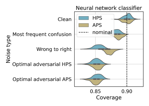
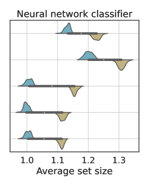
Figure A1: Effect of label noise on synthetic multi-class classification data. Performance of conformal prediction sets with target coverage $1-\alpha=90\%$, using a noisy training set and a noisy calibration set with adversarial noise models. Left: Marginal coverage; Right: Average size of predicted sets. The results are evaluated over 100 independent experiments.

A2.2 Synthetic regression: additional results

Here we first illustrate in Figure A2 the data we generate in the synthetic regression experiment and the different corruptions we apply.

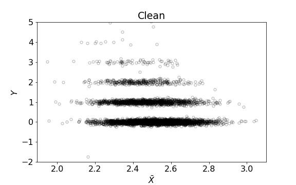
(a)

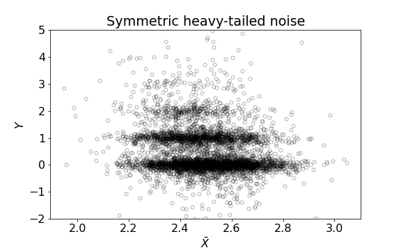
(b)

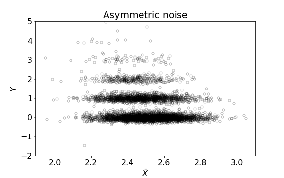
(c)

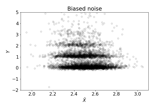
(d)

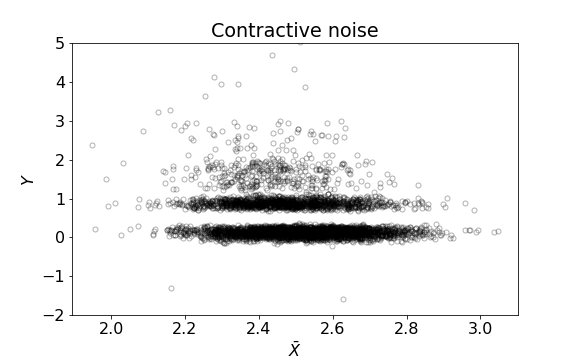
(e)

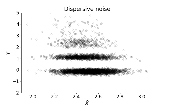
(f)

Figure A2: Illustration of the generated data with different corruptions. (a): Clean samples. (b): Samples with symmetric heavy-tailed noise. (c): Samples with asymmetric noise. (d): Samples with biased noise. Noise magnitude is set to 0.1. (e): Samples with contractive noise. (f): Samples with dispersive noise.

In Section 4.2 of the main manuscript we apply some realistic noise models and examine the performance of conformal prediction using CQR score with noisy training and calibration sets. Here we construct some more experiments using the same settings, however we train the models using clean data instead of noisy data. Moreover, we apply an additional adversarial noise model that differs from those presented in Section 4.2 in the sense that it is designed to intentionally reduce the coverage level.

Wrong to right: an adversarial noise that depends on the underlying trained regression model. In order to construct the noisy calibration set we switch 7% of the responses as follows: we randomly swap between outputs that are not included in the interval predicted by the model and outputs that are included.

Figures A3 and A4 depict the marginal coverage and interval length achieved when applying the different noise models. We see that the adversarial wrong to right noise model reduces the coverage rate to approximately 83%. Moreover, these results are similar to those achieved in Section 4.2, except for the conservative coverage attained using biased noise, which can be explained by the more accurate low and high estimated quantiles.

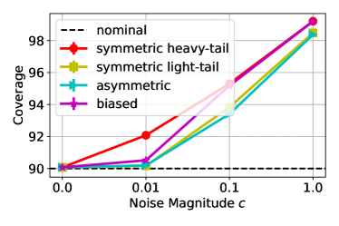
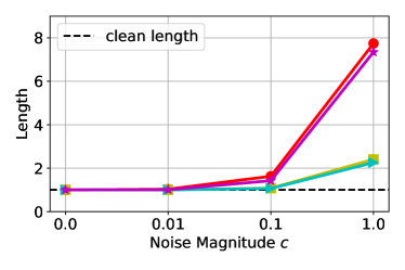
Figure A3: Response-independent noise. Performance of conformal prediction intervals with target coverage $1-\alpha=90\%$, using a clean training set and a noisy calibration set. Left: Marginal coverage; Right: Length of predicted intervals (divided by the average clean length) using symmetric, asymmetric and biased noise with a varying magnitude. Other details are as in Figure 7.

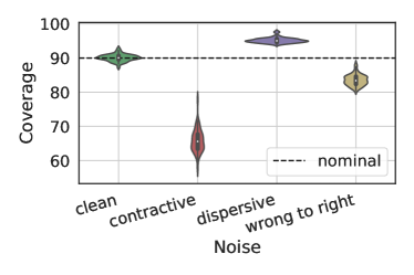
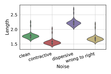
Figure A4: Response-dependent noise. Performance of conformal prediction intervals with target coverage $1-\alpha=90\%$, using a clean training set and a noisy calibration set. Left: Marginal coverage; Right: Length of predicted intervals. The results are evaluated over 50 independent experiments.

Lastly, in order to explain the over-coverage or under-coverage achieved for some of the different noise models, as depicted in Figures 7 and  8, we present in Figure A5 the CQR scores and their 90%’th empirical quantile. Over-coverage is achieved when the noisy scores are larger than the clean ones, for example, in the symmetric heavy tailed case, and under-coverage is achieved when the noisy scores are smaller.

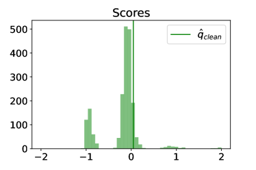
(a)

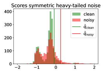
(b)

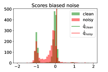
(c)

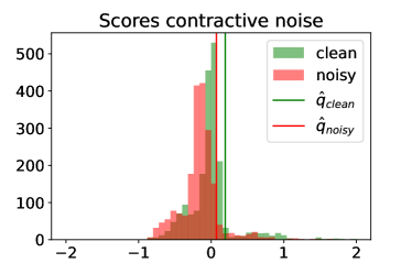
(d)

Figure A5: Illustration of the CQR scores. (a): Clean training and calibration sets. (b): Symmetric heavy-tailed noise. (c): Biased noise. Noise magnitude is set to 0.1. (d): Contractive noise. Other details are as in Figure 7.

A2.3 Regression: aesthetic visual rating

Herein, we provide additional details regarding the training of the predictive models for the real-world regression task. As explained in Section 2.2, we trained two different models in this experiment. The first is a quantile regression model for CQR. Here we trained the model for 70 epochs using ’SGD’ optimizer with a batch size of 128 and an initial learning rate of 0.001 decayed every 20 epochs exponentially with a rate of 0.95 and a frequency of 10. We applied dropout regularization to avoid overfitting with a rate of 0.2. The second model is a classic regression model for conformal with residual magnitude scores. Here we trained the model for 70 epochs using ’Adam’ optimizer with a batch size of 128 and an initial learning rate of 0.00005 decayed every 10 epochs exponentially with a rate of 0.95 and a frequency of 10. The dropout rate in this case is 0.5.

A2.4 Classification: object recognition experiment

Here we present additional results of the classification experiment with CIFAR-10H explained in Section 2.2, but first provide further details about the dataset and training procedure. The CIFAR-10H data set contains the same 10,000 images as CIFAR-10, but with labels from a single annotator instead of a majority vote of 50 annotators. We fine-tune a ResNet18 model pre-trained on the clean training set of CIFAR-10, which contains 50,000 samples. Then we randomly select 2,000 observations from CIFAR-10H for calibration. The test set contains the remaining 8,000 samples, but with CIFAR-10 labels. We apply conformal prediction with the APS score. The marginal coverage achieved when using noisy and clean calibration sets are depicted in Figure 1. This figure shows that (i) we obtain the exact desired coverage when using the clean calibration set; and (ii) when calibrating on noisy data, the constructed prediction sets over-cover the clean test labels. Figure A6 illustrates the average prediction set sizes that are larger when using noisy data for calibration and thus lead to higher coverage levels.

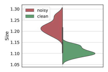
Figure A6: Effect of label noise on CIFAR-10. Distribution of average prediction set sizes over 30 independent experiments evaluated on CIFAR-10H test data using noisy and clean labels for calibration. Other details are as in Figure 1

A2.5 The multi-label classification experiment with the COCO dataset

Here, we provide the full details about the experimental setup of the real multi-label corruptions from Section 3.2. We asked 9 annotators to annotate 117 images. Each annotator labeled approximately 15 images separately, except for two annotators who labeled 15 images as a couple. The annotators were asked to label each image under 30 seconds, although this request was not enforced. Figure A7 presents the number of labels that are missed or mistakenly added to each image. On average, 1.25 of the labels were missed and 0.5 were mistakenly added, meaning that each image contains a total of 1.75 label mistakes on average.

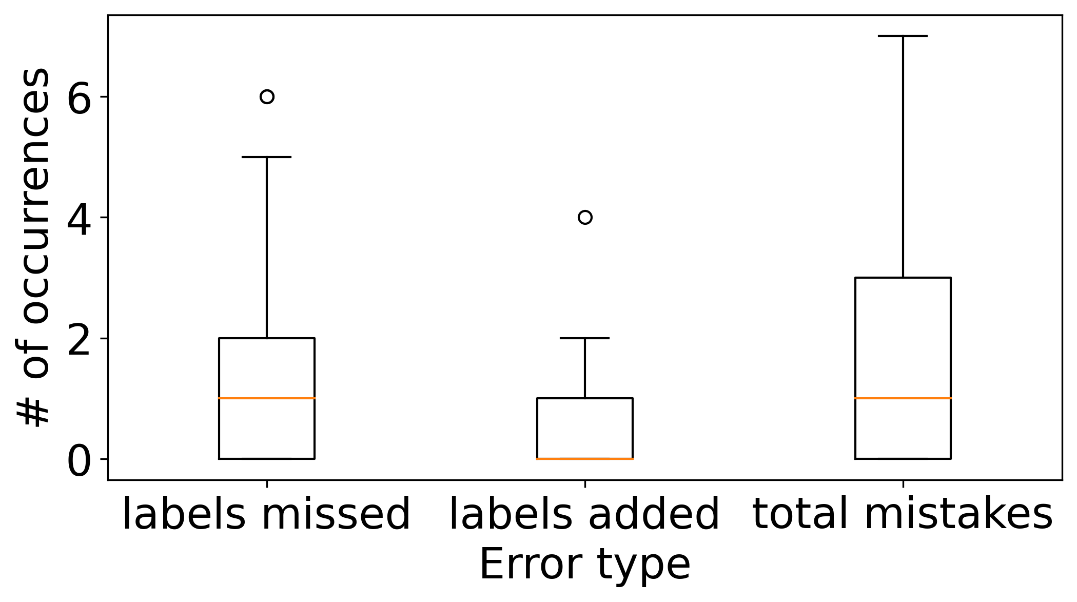
Figure A7: Analysis of human-made label corruptions in MS COCO dataset.

A2.6 Multi-label classification with artificial corruptions

In this section, we study three types of corruptions that demonstrate Proposition 3.1 in the sense that the number of positive labels, $|\tilde{Y}|$, is a deterministic function of $X$. The dataset we use in the following experiments is the MS COCO dataset (Lin et al., 2014), in which the input image may contain up to $K=80$ positive labels. We consider the given annotations as ground-truth labels and artificially corrupt them to generate noisy ones, as conducted in Zhao and Gomes (2021); Kumar et al. (2020). The first noise model applies dependent corruptions by taking $\beta$ of the positive labels and turning them into different ones, according to a pre-defined transition map that was randomly chosen. The second one applies independent corruptions: $\beta$ of the positive labels turn into different ones, chosen independently and uniformly. Finally, the partial noise model corrupts the labels as the independent one, except for 30 pre-defined labels that remain unchanged. In all experiments, we set $\beta=0.45$.

We fit a TResNet (Ridnik et al., 2021) model on 100k clean samples and calibrate it using 10K noisy samples with conformal risk control, as outlined in (Angelopoulos et al., 2022, Section 3.2). We control the false-negative rate (FNR), defined in (20), at different labels and measure the FNR obtained over clean and noisy versions of the test set which contains 30k samples. Figure A8 displays the results, showing that the risk obtained over the clean labels is more conservative than the risk of the clean labels. This is not a surprise, as it is supported by our theory, in Proposition 3.1.

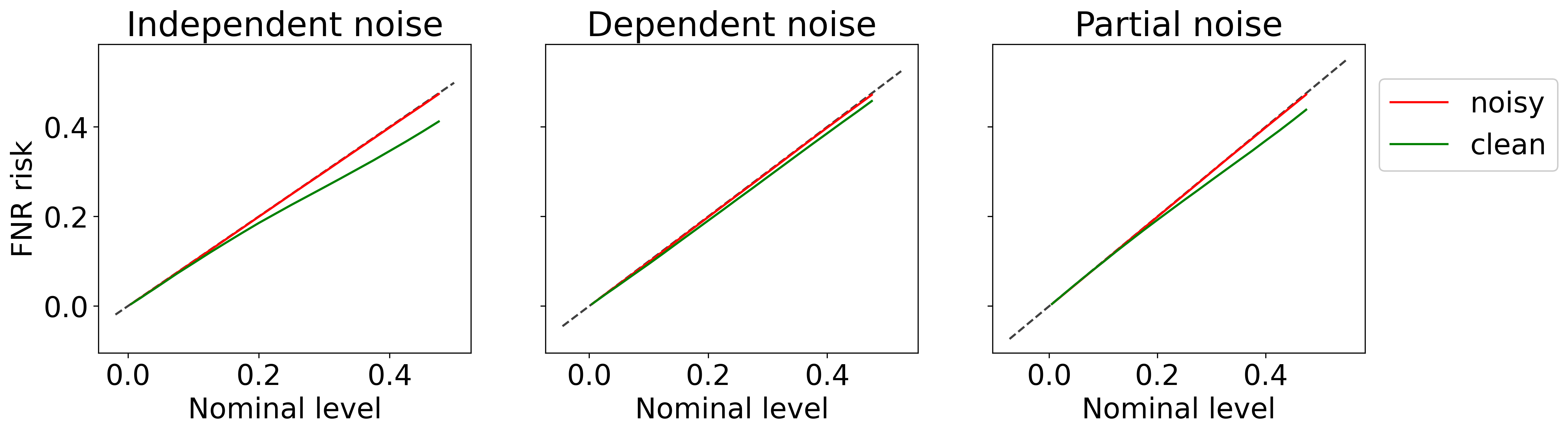
Figure A8: FNR on MS COCO dataset, achieved over noisy (red) and clean (green) test sets. The calibration scheme is applied with noisy annotations. Results are averaged over 50 trials.

A2.7 Regression miscoverage bounds experiment

We repeat the experimental protocol detailed in Section 4.5 with the same datasets and analyze the miscoverage bounds formulated in Section 3.3.3. Here, we apply conformalized quantile regression to control the miscoverage rate at different levels using a noisy calibration set. Furthermore, we choose the miscoverage bound hyperparameters, $c,d$, from (A42) by a grid search over the calibration set with the objective of tightening the miscoverage bound. Figure A9 displays the miscoverage rate achieved on the clean and noisy versions of the test set, along with the miscoverage bound. Importantly, in contrast to Theorem A2, this bound requires no assumptions on the distribution of $Y\mid X=x$ or on the distribution of the noise $\varepsilon$. The only requirement is that the noise is independent of the response variable and has mean $0$. This great advantage covers up for the looseness of the bound.

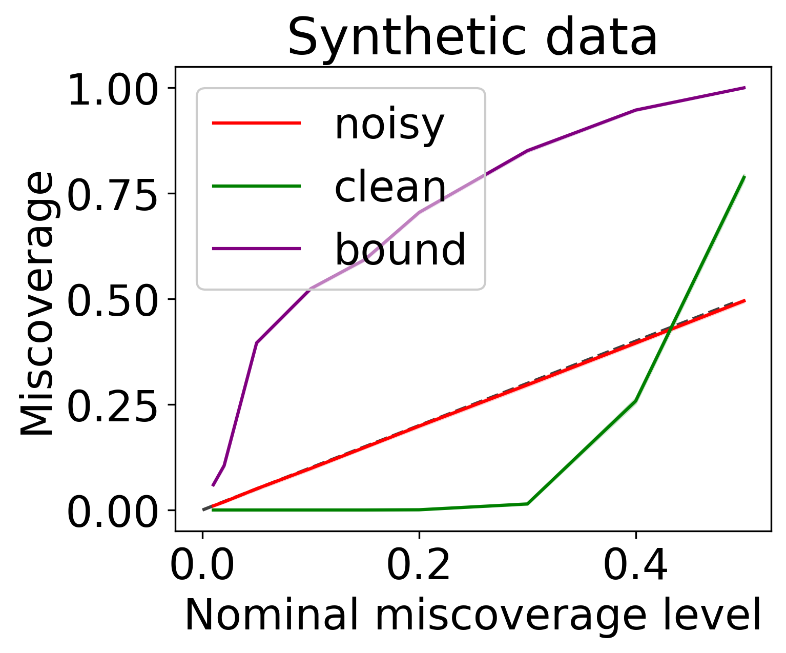
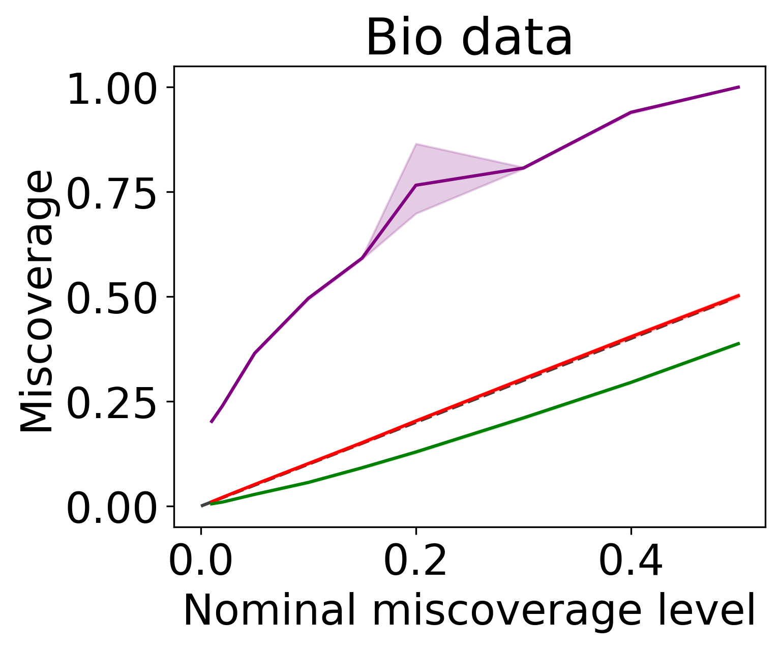
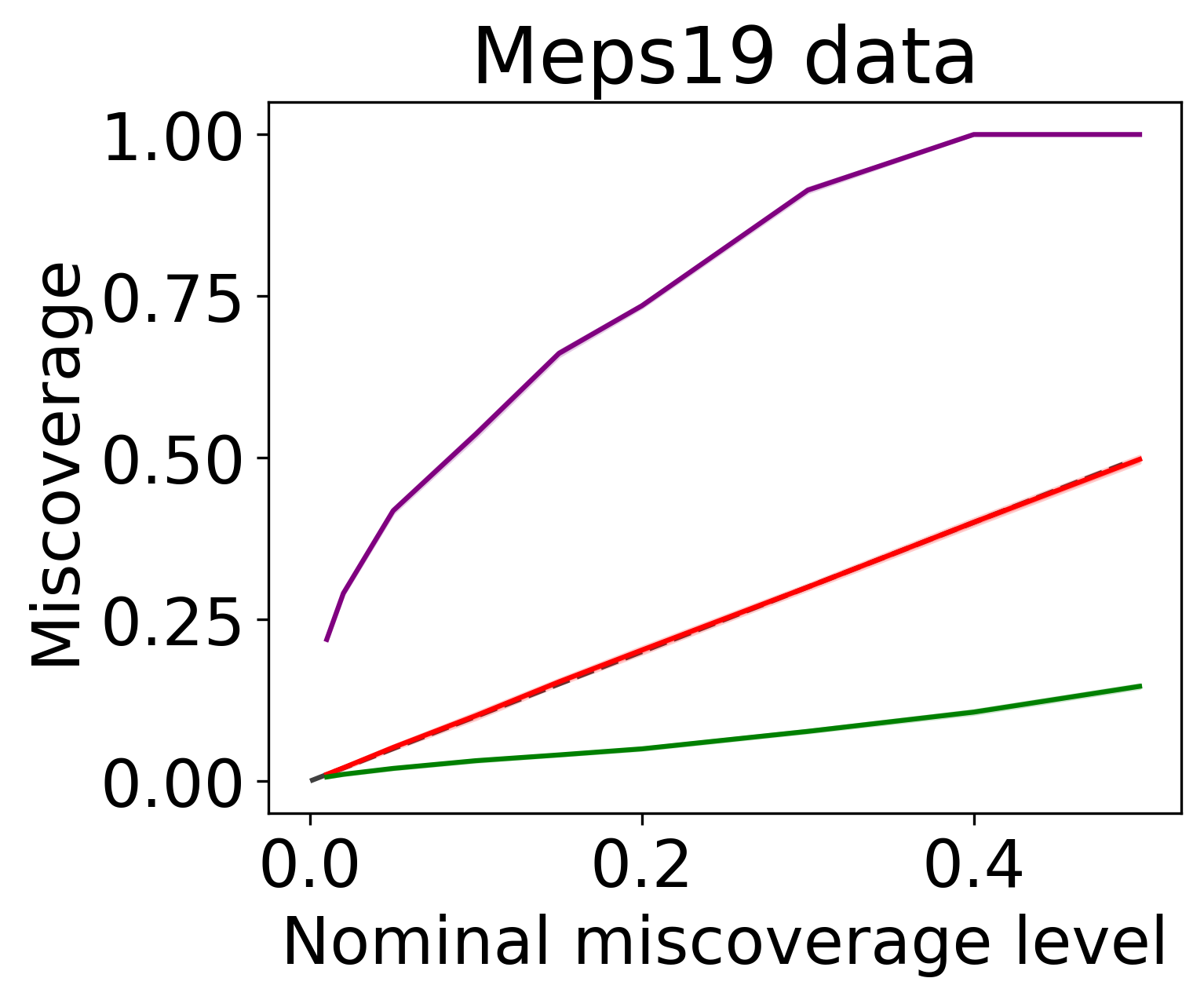
Figure A9: Miscoverage rate achieved over noisy (red) and clean (green) test sets. The calibration scheme is applied using noisy annotations to control the miscoverage level. Results are averaged over 10 random splits of the calibration and test sets.

References

- Algan and Ulusoy (2020) Görkem Algan and Ilkay Ulusoy. Label noise types and their effects on deep learning. arXiv preprint arXiv:2003.10471, 2020.
- Angelopoulos and Bates (2021) Anastasios N Angelopoulos and Stephen Bates. A gentle introduction to conformal prediction and distribution-free uncertainty quantification. arXiv preprint arXiv:2107.07511, 2021.
- Angelopoulos et al. (2021) Anastasios N. Angelopoulos, Stephen Bates, Emmanuel J. Candès, Michael I. Jordan, and Lihua Lei. Learn then test: Calibrating predictive algorithms to achieve risk control. arXiv preprint, 2021. arXiv:2110.01052.
- Angelopoulos et al. (2022) Anastasios N Angelopoulos, Stephen Bates, Adam Fisch, Lihua Lei, and Tal Schuster. Conformal risk control. arXiv preprint arXiv:2208.02814, 2022.
- Angluin and Laird (1988) Dana Angluin and Philip Laird. Learning from noisy examples. Machine Learning, 2(4):343–370, 1988.
- Aslam and Decatur (1996) Javed A Aslam and Scott E Decatur. On the sample complexity of noise-tolerant learning. Information Processing Letters, 57(4):189–195, 1996.
- Barber (2020) Rina Foygel Barber. Is distribution-free inference possible for binary regression? arXiv:2004.09477, 2020.
- Barber et al. (2021) Rina Foygel Barber, Emmanuel J Candès, Aaditya Ramdas, and Ryan J Tibshirani. Predictive inference with the jackknife+. The Annals of Statistics, 49(1):486 – 507, 2021.
- Barber et al. (2022) Rina Foygel Barber, Emmanuel J Candes, Aaditya Ramdas, and Ryan J Tibshirani. Conformal prediction beyond exchangeability. arXiv preprint arXiv:2202.13415, 2022.
- Bates et al. (2021) Stephen Bates, Anastasios Angelopoulos, Lihua Lei, Jitendra Malik, and Michael I. Jordan. Distribution-free, risk-controlling prediction sets. Journal of the ACM, 68(6), September 2021. ISSN 0004-5411.
- Battleday et al. (2020) Ruairidh M Battleday, Joshua C Peterson, and Thomas L Griffiths. Capturing human categorization of natural images by combining deep networks and cognitive models. Nature communications, 11(1):1–14, 2020.
- (12) bio. Physicochemical properties of protein tertiary structure data set. https://archive.ics.uci.edu/ml/datasets/Physicochemical+Properties+of+Protein+Tertiary+Structure. Accessed: January, 2019.
- Cauchois et al. (2022) Maxime Cauchois, Suyash Gupta, Alnur Ali, and John Duchi. Predictive inference with weak supervision. arXiv preprint arXiv:2201.08315, 2022.
- Cheng et al. (2022) Chen Cheng, Hilal Asi, and John Duchi. How many labelers do you have? a closer look at gold-standard labels. arXiv preprint arXiv:2206.12041, 2022.
- Fan et al. (2020) Deng-Ping Fan, Ge-Peng Ji, Tao Zhou, Geng Chen, Huazhu Fu, Jianbing Shen, and Ling Shao. Pranet: Parallel reverse attention network for polyp segmentation. In International conference on medical image computing and computer-assisted intervention, pages 263–273. Springer, 2020.
- Feldman et al. (2022) S Feldman, L Ringel, S Bates, and Y Romano. Achieving risk control in online learning settings. arXiv preprint arXiv:2205.09095, 2022.
- Frénay and Verleysen (2013) Benoît Frénay and Michel Verleysen. Classification in the presence of label noise: a survey. IEEE transactions on neural networks and learning systems, 25(5):845–869, 2013.
- Geiger et al. (2013) Andreas Geiger, Philip Lenz, Christoph Stiller, and Raquel Urtasun. Vision meets robotics: The kitti dataset. International Journal of Robotics Research (IJRR), 2013.
- Gendler et al. (2021) Asaf Gendler, Tsui-Wei Weng, Luca Daniel, and Yaniv Romano. Adversarially robust conformal prediction. In International Conference on Learning Representations, 2021.
- Gibbs and Candes (2021) Isaac Gibbs and Emmanuel Candes. Adaptive conformal inference under distribution shift. In A. Beygelzimer, Y. Dauphin, P. Liang, and J. Wortman Vaughan, editors, Advances in Neural Information Processing Systems, 2021.
- Jenni and Favaro (2018) Simon Jenni and Paolo Favaro. Deep bilevel learning. In Proceedings of the European conference on computer vision (ECCV), pages 618–633, 2018.
- Jindal et al. (2016) Ishan Jindal, Matthew Nokleby, and Xuewen Chen. Learning deep networks from noisy labels with dropout regularization. In 2016 IEEE 16th International Conference on Data Mining (ICDM), pages 967–972. IEEE, 2016.
- Kao et al. (2015) Yueying Kao, Chong Wang, and Kaiqi Huang. Visual aesthetic quality assessment with a regression model. In 2015 IEEE International Conference on Image Processing (ICIP), pages 1583–1587. IEEE, 2015.
- Kumar et al. (2020) Himanshu Kumar, Naresh Manwani, and PS Sastry. Robust learning of multi-label classifiers under label noise. In Proceedings of the 7th ACM IKDD CoDS and 25th COMAD, pages 90–97. 2020.
- Lee and Barber (2022) Yonghoon Lee and Rina Foygel Barber. Binary classification with corrupted labels. Electronic Journal of Statistics, 16(1):1367 – 1392, 2022.
- Lei et al. (2013) Jing Lei, James Robins, and Larry Wasserman. Distribution-free prediction sets. Journal of the American Statistical Association, 108(501):278–287, 2013.
- Lei et al. (2018) Jing Lei, Max G’Sell, Alessandro Rinaldo, Ryan J. Tibshirani, and Larry Wasserman. Distribution-free predictive inference for regression. Journal of the American Statistical Association, 113(523):1094–1111, 2018.
- Lin et al. (2014) Tsung-Yi Lin, Michael Maire, Serge Belongie, James Hays, Pietro Perona, Deva Ramanan, Piotr Dollár, and C Lawrence Zitnick. Microsoft COCO: Common objects in context. In European conference on computer vision, pages 740–755. Springer, 2014. doi: 10.1007/978-3-319-10602-1˙48.
- Ma et al. (2018) Xingjun Ma, Yisen Wang, Michael E Houle, Shuo Zhou, Sarah Erfani, Shutao Xia, Sudanthi Wijewickrema, and James Bailey. Dimensionality-driven learning with noisy labels. In International Conference on Machine Learning, pages 3355–3364. PMLR, 2018.
- meps_ (19) meps_19. Medical expenditure panel survey, panel 19. https://meps.ahrq.gov/mepsweb/data_stats/download_data_files_detail.jsp?cboPufNumber=HC-181. Accessed: January, 2019.
- Murray et al. (2012) Naila Murray, Luca Marchesotti, and Florent Perronnin. Ava: A large-scale database for aesthetic visual analysis. In 2012 IEEE conference on computer vision and pattern recognition, pages 2408–2415. IEEE, 2012.
- Peterson et al. (2019) Joshua C Peterson, Ruairidh M Battleday, Thomas L Griffiths, and Olga Russakovsky. Human uncertainty makes classification more robust. In Proceedings of the IEEE/CVF International Conference on Computer Vision, pages 9617–9626, 2019.
- Podkopaev and Ramdas (2021) Aleksandr Podkopaev and Aaditya Ramdas. Distribution-free uncertainty quantification for classification under label shift. In Uncertainty in Artificial Intelligence, pages 844–853. PMLR, 2021.
- Ridnik et al. (2021) Tal Ridnik, Hussam Lawen, Asaf Noy, Emanuel Ben Baruch, Gilad Sharir, and Itamar Friedman. Tresnet: High performance gpu-dedicated architecture. In proceedings of the IEEE/CVF winter conference on applications of computer vision, pages 1400–1409, 2021.
- Romano et al. (2019) Yaniv Romano, Evan Patterson, and Emmanuel Candès. Conformalized quantile regression. In Advances in Neural Information Processing Systems, volume 32, pages 3543–3553. 2019.
- Romano et al. (2020) Yaniv Romano, Matteo Sesia, and Emmanuel Candès. Classification with valid and adaptive coverage. In Advances in Neural Information Processing Systems, volume 33, pages 3581–3591, 2020.
- Singh et al. (2020) Pulkit Singh, Joshua C Peterson, Ruairidh M Battleday, and Thomas L Griffiths. End-to-end deep prototype and exemplar models for predicting human behavior. arXiv preprint arXiv:2007.08723, 2020.
- Talebi and Milanfar (2018) Hossein Talebi and Peyman Milanfar. NIMA: Neural image assessment. IEEE transactions on image processing, 27(8):3998–4011, 2018.
- Tanno et al. (2019) Ryutaro Tanno, Ardavan Saeedi, Swami Sankaranarayanan, Daniel C Alexander, and Nathan Silberman. Learning from noisy labels by regularized estimation of annotator confusion. In Proceedings of the IEEE/CVF conference on computer vision and pattern recognition, pages 11244–11253, 2019.
- Tibshirani et al. (2019) Ryan J Tibshirani, Rina Foygel Barber, Emmanuel Candes, and Aaditya Ramdas. Conformal prediction under covariate shift. In Advances in Neural Information Processing Systems, volume 32, pages 2530–2540. 2019.
- Vovk (2015) Vladimir Vovk. Cross-conformal predictors. Annals of Mathematics and Artificial Intelligence, 74(1-2):9–28, 2015.
- Vovk et al. (1999) Vladimir Vovk, Alexander Gammerman, and Craig Saunders. Machine-learning applications of algorithmic randomness. In International Conference on Machine Learning, pages 444–453, 1999.
- Vovk et al. (2005) Vladimir Vovk, Alex Gammerman, and Glenn Shafer. Algorithmic Learning in a Random World. Springer, New York, NY, USA, 2005.
- Wei et al. (2022) Jiaheng Wei, Zhaowei Zhu, Hao Cheng, Tongliang Liu, Gang Niu, and Yang Liu. Learning with noisy labels revisited: A study using real-world human annotations. In International Conference on Learning Representations, 2022. URL https://openreview.net/forum?id=TBWA6PLJZQm.
- Xu et al. (2019) Yilun Xu, Peng Cao, Yuqing Kong, and Yizhou Wang. L_dmi: A novel information-theoretic loss function for training deep nets robust to label noise. Advances in neural information processing systems, 32, 2019.
- Yin et al. (2021) Wei Yin, Jianming Zhang, Oliver Wang, Simon Niklaus, Long Mai, Simon Chen, and Chunhua Shen. Learning to recover 3d scene shape from a single image. In Proceedings of the IEEE/CVF Conference on Computer Vision and Pattern Recognition, pages 204–213, 2021.
- Yuan et al. (2018) Bodi Yuan, Jianyu Chen, Weidong Zhang, Hung-Shuo Tai, and Sara McMains. Iterative cross learning on noisy labels. In 2018 IEEE Winter Conference on Applications of Computer Vision (WACV), pages 757–765. IEEE, 2018.
- Zhao and Gomes (2021) Wenting Zhao and Carla Gomes. Evaluating multi-label classifiers with noisy labels. arXiv preprint arXiv:2102.08427, 2021.