Global Speed Limit for Finite-Time Dynamical Phase Transition and Nonequilibrium Relaxation

Abstract

Recent works unraveled an intriguing finite-time dynamical phase transition in the thermal relaxation of the mean field Curie-Weiss model. The phase transition reflects a sudden switch in the dynamics. Its existence in systems with a finite range of interaction, however, remained unclear. Here we demonstrate the dynamical phase transition for nearest-neighbor Ising systems on the square and Bethe lattices through extensive computer simulations and by analytical results. Combining large-deviation techniques and Bethe-Guggenheim theory we prove the existence of the dynamical phase transition for arbitrary quenches, including those within the two-phase region. Strikingly, for any given initial condition we prove and explain the existence of non-trivial speed limits for the dynamical phase transition and the relaxation of magnetization, which are fully corroborated by simulations of the microscopic Ising model but are absent in the mean field setting. Pair correlations, which are neglected in mean field theory and trivial in the Curie-Weiss model, account for kinetic constraints due to frustrated local configurations that give rise to a global speed limit.

Despite its overwhelming importance in condensed matter physics Dattagupta (2012); Wolfgang Haase (2003), our understanding of thermal relaxation kinetics is far from complete and mostly limited to systems near equilibrium Onsager (1931a, b); Kubo et al. (1957) and non-equilibrium Seifert and Speck (2010); Baiesi and Maes (2013); Wu and Wang (2020) steady states. Notable advances in understanding relaxation dynamics out of equilibrium include far-from-equilibrium fluctuation-dissipation theorems Cugliandolo et al. (1997); Lippiello et al. (2014), “frenesy” Maes (2020), anomalous relaxation a.k.a. the Mpemba effect Lu and Raz (2017); Klich et al. (2019); Lasanta et al. (2017); Busiello et al. (2021); Holtzman and Raz (2022), optimal heating and cooling Gal and Raz (2020) as well as driving Zulkowski and DeWeese (2015); Frim et al. (2021) protocols, asymmetries in heating and cooling rates Lapolla and Godec (2020); Meibohm et al. (2021); Manikandan (2021); Van Vu and Hasegawa (2021), and dynamical phase transitions (i.e. the occurence of non-analytic points in distributions of physical observables) Graham and Tél (1984, 1985); Bouchet et al. (2016); Bertini et al. (2001, 2010); Bunin et al. (2012, 2013); Baek and Kafri (2015); Garrahan et al. (2007, 2009); Chandler and Garrahan (2010); Garrahan and Lesanovsky (2010); Ates et al. (2012); Hickey et al. (2014); Jack and Sollich (2013); Gorissen et al. (2012); Espigares et al. (2013); Tsobgni Nyawo and Touchette (2016a); Tizón-Escamilla et al. (2017); Mehl et al. (2008); Speck et al. (2012); Tsobgni Nyawo and Touchette (2016b); Jack et al. (2015); Harris and Touchette (2017); Barratt et al. (2021). Further important results on non-equilibrium relaxation are embodied in thermodynamic uncertainty relations for non-stationary systems Pietzonka et al. (2017); Dechant (2018); Liu et al. (2020); Koyuk and Seifert (2019, 2020); Dieball and Godec (2022), and so called speed limits Mandelstam and Tamm (1945); Bhattacharyya (1983); Anandan and Aharonov (1990); Pfeifer (1993); Margolus and Levitin (1998); Lloyd (2000); Giovannetti et al. (2003); Pfeifer (1993); Deffner and Lutz (2013a); Taddei et al. (2013); del Campo et al. (2013); Deffner and Lutz (2013b); García-Pintos et al. (2022); Okuyama and Ohzeki (2018); Shanahan et al. (2018); Shiraishi et al. (2018); Aurell et al. (2011); Ito and Dechant (2020); Aurell et al. (2012); Vo et al. (2020); Falasco and Esposito (2020); Ito and Dechant (2020); Shiraishi and Saito (2019); Yoshimura and Ito (2021).

In contrast to the well established concept of quantum speed limits Mandelstam and Tamm (1945); Bhattacharyya (1983); Anandan and Aharonov (1990); Pfeifer (1993); Margolus and Levitin (1998); Lloyd (2000); Giovannetti et al. (2003); Pfeifer (1993); Deffner and Lutz (2013a); Taddei et al. (2013); del Campo et al. (2013); Deffner and Lutz (2013b); García-Pintos et al. (2022) that has long been known Mandelstam and Tamm (1945), it was comparably only recently found that the evolution of classical systems is also bounded by fundamental speed limits Okuyama and Ohzeki (2018); Shanahan et al. (2018); Shiraishi et al. (2018); Aurell et al. (2011); Ito and Dechant (2020); Aurell et al. (2012); Vo et al. (2020). Quantum and classical speed-limits impose an upper bound on the rate of change of a system state evolving from a given non-stationary initial state, and arise as an intrinsic dynamical property of Hilbert space Okuyama and Ohzeki (2018). Moreover, it was found that by considering the thermodynamic cost of the state change one may derive even sharper thermodynamic speed limits that bound the rate of change of a system state from above by the entropy production rate Shiraishi et al. (2018); Falasco and Esposito (2020); Ito and Dechant (2020); Shiraishi and Saito (2019); Yoshimura and Ito (2021).

Recently, a surprising finite-time dynamical phase transition was observed in a mean field (MF) Ising system Meibohm and Esposito (2022, 2023), manifested as a finite-time singularity Külske and Le Ny (2007); Ermolaev and Külske (2010) in the probability density of magnetization Meibohm and Esposito (2022) and entropy flow per spin Meibohm and Esposito (2023) upon a quench from any sub-critical temperature $T<T_{c}$ to a temperature $T_{q}$ . In contrast to conventional phase transitions, here time plays the role of a control parameter inducing an abrupt change of the typical dynamics Meibohm and Esposito (2022, 2023). The sudden transition from a Gibbsian to a non-Gibbsian probability density occurs for all quenches from sub-critical temperatures $T<T_{c}$, whereby the initial location of the singularity depends on $T$ and $T_{q}$ Ermolaev and Külske (2010). Upon quenches from super-critical temperatures $T>T_{c}$ the probability density remains Gibbsian forever Ermolaev and Külske (2010), but the dynamics is non-ergodic Bray (1993).

Notwithstanding the detailed results on the non-Gibbsian transition in the MF setting, it remains unknown if and in what form this novel dynamical phase transition exists in systems with a finite range of interactions. Moreover, since speed limits bound from below the time of reaching a final state from a given initial state, the following intriguing questions arise: What happens with the speed limit in the finite-time dynamical phase transition, where the dynamics experiences an abrupt change? Is there a global speed limit to reaching the critical time?

To shed light on these questions we here present analytical results on non-equilibrium relaxation of nearest-neighbor Ising systems on the Bethe-Guggenheim (BG) level Bethe (1935); Guggenheim (1935), which accounts for nearest-neighbor pair correlations and is exact for the nearest-neighbor Ising model on the Bethe lattice. Furthermore, we present circumstantial simulation evidence for the dynamical phase transition on the square and Bethe lattices. Our results confirm, for the first time, the existence of the finite-time dynamical phase transition in finite-range Ising systems. Strikingly, we derive explicit global speed limits to both, the critical time and relaxation time, on the Bethe and square lattices, which are fully corroborated by simulations of the full Ising model but are absent in the MF setting. Notably, the speed limit is set by an antiferromagnetic interaction and is faster than the dynamics of a non-interacting system. Accounting for kinetically unfavorable local spin configurations, pair correlations, which are neglected in MF theory, impose a global speed limit on the non-Gibbsian dynamical phase transition.

Fundamentals.—The Hamiltonian of nearest-neighbor interacting Ising spins $\sigma_{i}=\pm 1,\ i=\{1,...,N\}$ reads

$$H(\boldsymbol{\sigma},J)=-J\sum_{\langle ij\rangle}\sigma_{i}\sigma_{j},$$ (1)

with $J$ denoting the ferromagnetic ($J>0$) or antiferromagnetic ($J<0$) coupling and $\langle ij\rangle$ the sum over nearest neighbor spin pairs. The spins are placed on a Bethe lattice with coordination number $\bar{z}\in\mathbb{N}^{+}$. Let $m(\boldsymbol{\sigma})\equiv N^{-1}\sum_{i=1}^{N}\sigma_{i}$ be the magnetization per spin for a given configuration $\boldsymbol{\sigma}=(\sigma_{1},...,\sigma_{N})$. The equilibrium free energy density in the thermodynamic limit is defined as ${\rm f}(m;J)=-\lim^{m={\rm const.}}_{N\rightarrow\infty}\left[N^{-1}\ln{(\mathcal{Z}_{m}(J))}\right]$, where $\mathcal{Z}_{k}(J)\equiv\sum_{\boldsymbol{\sigma}}\exp{(-H(\boldsymbol{\sigma},J)/k_{\rm B}T)}\mathbbm{1}_{m(\boldsymbol{\sigma}),k}$ is the fixed-magnetization partition function with indicator function $\mathbbm{1}_{a,b}$ being 1 when $a=b$ and $0$ otherwise. Within BG theory, the free energy density in units of $k_{\rm B}T$, $\tilde{\rm f}_{\rm BG}\equiv{\rm f}_{\rm BG}/k_{\rm B}T$, reads (exactly for Bethe lattices) Blom and Godec (2021); Bethe (1935); Guggenheim (1935)

$$\tilde{\rm f}_{\rm BG}(m;\tilde{J}) = \bar{z}\tilde{J}(\zeta(m;\tilde{J})-1/2){+}(1{-}\bar{z})[\Xi(m)+\Xi(-m)]$$ (2)

$$+ \frac{\bar{z}}{2}\sum_{\eta=\pm}[\Xi(\eta m{-}\zeta(m;\tilde{J}))+\Xi(\zeta(m;\tilde{J}){-}1)],$$

where $\Xi(m)\equiv(1/2{+}m/2)\ln{(1/2{+}m/2)}$, ${\tilde{J}{\equiv}J/k_{\rm B}}T$, and

$$\zeta(m;\tilde{J})\equiv\frac{1-m^{2}}{1+[m^{2}+\exp(4\tilde{J})(1-m^{2})]^{1/2}}.$$ (3)

The MF counterpart is recovered by applying the transformation $\zeta(m;\tilde{J})\rightarrow(1-m^{2})/2$, or equivalently to setting $\tilde{J}=0$ in Eq. (3) . The BG critical temperature below which $\tilde{\rm f}_{\rm BG}(m;\tilde{J})$ develops two degenerate minima reads $\tilde{J}^{\rm BG}_{c}\equiv\ln{(\bar{z}/(\bar{z}-2))}/2$, and correctly diverges in dimension one with $\bar{z}=2$, where no phase transition occurs. An exact result for ${\rm f}(m;\tilde{J})$ on the square lattice remains elusive McCoy and Maillard (2012), while the critical temperature reads $\tilde{J}^{\rm SQ}_{c}\equiv\ln{(1+\sqrt{2})}/2$ Onsager (1944).

We focus on the magnetization $m$ evolving under Glauber dynamics of $\boldsymbol{\sigma}$ Glauber (1963); Blom and Godec (2021) upon an instantaneous temperature quench ${\tilde{J}_{0}\rightarrow\tilde{J}_{q}<\tilde{J}_{0}}$, where $\tilde{J}_{q}$ may be positive or negative. Let $P_{N}(m;\tilde{J},t)$ be the probability density of $m$ at time $t$ and ${V_{N}(m;\tilde{J},t)\equiv-N^{-1}\ln P_{N}(m;\tilde{J},t)}$ the time-dependent large-deviation rate function. We set $V(m;\tilde{J},t)\equiv\lim^{m={\rm const.}}_{N\rightarrow\infty}V_{N}(m;\tilde{J},t)$. At equilibrium we have $V_{\rm eq}(m;\tilde{J})\equiv\lim_{t\to\infty}V(m;\tilde{J},t)=\tilde{\rm f}(m;\tilde{J})-\tilde{\rm f}(\bar{m};\tilde{J})$ with $\bar{m}(\tilde{J})\equiv\arg\min_{m}\tilde{\rm f}(m;\tilde{J})$ denoting the location of free-energy minima. We are interested in the temporal evolution of $V(m;\tilde{J},t)$ upon applying the temperature quench. Experimentally quenches to negative $\tilde{J}_{q}$ may be achieved, e.g. by ultrafast optical switching ferro-antiferromagnetic materials Chatterjee et al. (2022) or by spin-population inversion in metals by radio-frequency irradiation Hakonen and Lounasmaa (1994) yielding negative spin temperatures . Note that quenches beyond the Néel point (i.e. the antiferromagnetic critical point) push the system across the antiferromagnetic transition, which $m$ does not detect Ziman (1951); Katsura and Takizawa (1974); Ono (1984); Peruggi et al. (1983). In fact, applying the reverse quench and replacing $m$ with the staggered magnetization Ziman (1951); Katsura and Takizawa (1974); Ono (1984); Peruggi et al. (1983) yields mirror-symmetric results (see Note (4)).

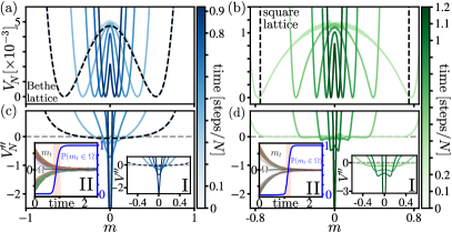
Figure 1: Kinetic Monte-Carlo (MC) simulations of the temporal evolution of $V_{N}(m;\tilde{J},t)$ (a-b) and $V_{N}^{\prime\prime}(m;\tilde{J},t)$ (c-d) for a Bethe ($\bar{z}=5,N=2000$) (a,c) and square lattice ($N{=}90\times 90$) (b,d) upon a quench from $\tilde{J}_{0}=0.275$ (Bethe) and $\tilde{J}_{0}=0.45$ (square) to an antiferromagnetic $\tilde{J}_{q}=-0.2$ (see Note (4) for simulation details). Time is expressed as the number of MC steps per spin, and increases from bright to dark. Black dashed lines show the initial equilibrium $V(m;\tilde{J}_{q},0)$ in Eq. (2) (a) and the minima of $V(m;\tilde{J}_{q},0)$ given by Onsager’s spontaneous magnetization Yang (1952) (b). Inset I: Theoretical evolution of $V^{\prime\prime}(m;\tilde{J},t)$ for a lattice with $\bar{z}=5$ (c) and $\bar{z}=4$ (d); profiles are shown at equal times as for simulations, but with ${\rm MC\ steps}/N$ replaced by $t/\tau_{r}$, where $\tau_{r}$ is the relaxation time (see text). Inset II: Trajectories of the magnetization $m_{t}$ (coloured lines) and the occupation probability $\mathbbm{P}(m_{t}\in\Omega)$ (blue lines) with $\Omega\equiv[-\epsilon,\epsilon]$ with $\epsilon=0.065$ (left) and $\epsilon=0.04$ (right).

Simulations.— We performed discrete-time single spin-flip Glauber Glauber (1963); Blom and Godec (2021) Monte Carlo (MC) simulations of the Ising model on the Bethe ($N=2000,\ \bar{z}=5$) and square lattice ($N=90\times 90$), MF results are shown in Note (4). Simulations on the Bethe lattice were performed with the random graph algorithm Johnston and Plechác (1998); Dhar et al. (1997). Starting from a random configuration with $m=0$ we equilibrated the system at temperature $\tilde{J}_{0}>\tilde{J}_{c}$. Upon complete equilibration (see Note (4) for benchmarks) we changed the temperature to $\tilde{J}_{q}$ and let the system relax. The magnetization was sampled at different time points and histograms and corresponding rate functions (see Fig. 1a-b) were determined from an ensemble of $4\times 10^{8}$ (Bethe) and $10^{8}$ (square) independent trajectories.

A clear signature that initial equilibration was complete is the agreement of the initial rate function with Eq. (2) for the Bethe lattice (Fig. 1a; black dashed line). Note that the small offset of the barrier diminishes for increasing system size (see Note (4)). Similarly, the minima of the initial rate function for the square lattice match Onsager’s spontaneous magnetization Yang (1952) (Fig. 1b; vertical black dashed line), where the agreement steadily improves for growing system sizes (see Note (4)).

Following $V_{N}$ in time we observe the occurrence of a peak at $m=0$ (see Fig. 1a-b). To evaluate this systematically, we determine the local curvature $V_{N}^{\prime\prime}$ (see Fig. 1c-d and Note (4) for details). Indeed, at some point the curvature near $m=0$ rapidly drops to large negative values, thus providing the first circumstantial evidence for the finite-time dynamical phase transition in nearest-neighbor Ising systems. The abrupt appearance of a true singularity is, of course, precluded by the finite system size. The simulated curvature profiles agree qualitatively with theoretical predictions in the $N\to\infty$ limit where the singularity indeed emerges (see Fig. 1c-d inset I).

Theory.— To go beyond finite-system MC simulations, we determined the temporal evolution of $V(m;\tilde{J},t)$ within the local equilibrium approximation Kawasaki (1966); Kadanoff and Swift (1968), which is highly accurate in the thermodynamic limit Blom and Godec (2021). Let $W^{\pm}(M;\tilde{J})$ denote the transition rate to change the total magnetization from $M\equiv Nm\rightarrow M\pm 2$ by a single-spin flip. Following Kawasaki (1966); Kadanoff and Swift (1968) we define, in the thermodynamic limit, an intensive transition rate $w^{\pm}(m;\tilde{J})\equiv\lim^{m={\rm const.}}_{N\rightarrow\infty}[W^{\pm}(Nm;\tilde{J})/N]$, which reads

$$w_{{\rm BG}}^{\pm}(m;\tilde{J})=\frac{1\mp m}{2\tau}\left(\mathrm{e}^{-\tilde{J}}+\frac{2\zeta(m;\tilde{J})\sinh{(\tilde{J}})}{1\mp m}\right)^{\bar{z}},$$ (4)

$\tau$ being an intrinsic time-scale of infinitesimal changes of magnetization $m\to m+\mathrm{d}m$ Saito and Kubo (1976). The transition rates obey the parity symmetry $w^{\pm}_{\rm BG}(m;\tilde{J})=w^{\mp}_{\rm BG}(-m;\tilde{J})$ and detailed balance w.r.t. the free energy density, $w^{+}_{\rm BG}(m;\tilde{J})/w^{-}_{\rm BG}(m;\tilde{J})=\exp{(-2\partial_{m}\tilde{\rm f}_{\rm BG}(m;\tilde{J}))}$. In the weak coupling (or high temperature) limit we recover MF rates $\lim_{\tilde{J}\rightarrow 0}w^{\pm}_{\rm BG}(m;\tilde{J})=w^{\pm}_{\rm MF}(m;\tilde{J})+\mathcal{O}(\tilde{J}^{2})$ reported in Meibohm and Esposito (2022). Out of equilibrium the rate function $V(m;\tilde{J},t)$ obeys a Hamilton-Jacobi equation Meibohm and Esposito (2022); Dykman et al. (1994); Imparato and Peliti (2005)

$$\partial_{t}V(m;\tilde{J},t)+\mathcal{H}(m,\partial_{m}V(m;\tilde{J},t))=0,$$ (5)

with the Hamiltonian given by

$$\mathcal{H}(q,p)=w^{+}(q;\tilde{J})(\mathrm{e}^{2p}-1)+w^{-}(q;\tilde{J})(\mathrm{e}^{-2p}-1).$$ (6)

Eq. (5) can be derived from the master equation for $P_{N}$ as the instanton solution in the thermodynamic limit.

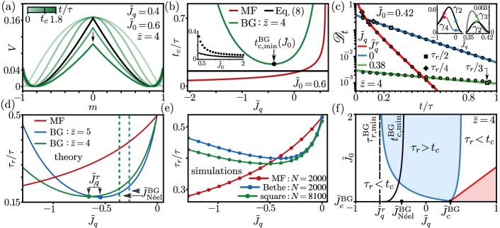
Figure 2: (a) Temporal evolution of the BG rate function $V(m;\tilde{J}_{q},t)$ upon a quench into the two-phase domain. (b) Critical time $t_{c}/\tau$ as a function of $\tilde{J}_{q}$ for BG (green) and MF (red) theory. The BG critical time attains a global minimum $t^{\rm BG}_{c,{\rm min}}$ (black dot) for an antiferromagnetic quench, bounded from below by Eq. (8) (black line); Inset: $t^{\rm BG}_{c,{\rm min}}$ (black dots) and Eq. (8) (black line) as a function of $\tilde{J}_{0}$. (c) Temporal evolution of the relative entropy per spin $\mathscrsfs{D}_{t}$ upon a quench into the one-phase (red and blue) and two-phase regime (green). At $\tilde{J}^{r}_{q}$ (red; Eq. (10)) the relative entropy relaxes the fastest. Dots depict analytical results obtained with the first two nonzero terms in Eq. (9). Lines correspond to numerical results. Squares/diamonds denote the first $\tau_{r}/2$ and second $\tau_{r}/4$ - $\tau_{r}/3$ relaxation time-scales, respectively. Inset: First two nonzero prefactors $\gamma_{k}$ which enter Eq. (9). (d) BG ($\bar{z}=4$ green, $\bar{z}=5$ blue) and MF (red) relaxation time $\tau_{r}/\tau$ as a function of $\tilde{J}_{q}$. The BG relaxation time has a local minimum at $\tilde{J}^{r}_{q}<0$ (see Eq. (10)). (e) Kinetic MC results of the relaxation time $\tau_{r}/\tau$ for the Bethe lattice with $\bar{z}=5$ (blue), square lattice (green), and MF lattice (red); see Note (4) for simulation details. (f) Dynamical phase diagram for $t^{\rm BG}_{c}$ and $\tau^{\rm BG}_{r}$. The red area is forbidden since $\tilde{J}_{0}>\tilde{J}_{q}$. Dashed/solid black lines denote the fastest relaxation and critical time.

Dynamical phase transition.—We assume that the system is initially prepared at equilibrium in the two-phase regime $\tilde{J}_{0}>\tilde{J}^{\rm BG}_{c}$ (i.e. below the Curie temperature), and thus $V_{\rm BG}(m;\tilde{J},0)=\tilde{\rm f}_{\rm BG}(m;\tilde{J}_{0}){-}\tilde{\rm f}_{\rm BG}(\bar{m};\tilde{J}_{0})$. At $t=0$ we apply an instantaneous quench $\tilde{J}_{q}<\tilde{J}_{0}$ whereupon $V_{\rm BG}(m;\tilde{J},t>0)$ evolves according to Eq. (5), which we solve numerically (see Fig. 2a for a quench with $\tilde{J}_{q}\geq\tilde{J}^{\rm BG}_{c}$). As $V_{\rm BG}(m;\tilde{J},t)$ relaxes, there is a defined moment $t^{\rm BG}_{c}(\tilde{J}_{0},\tilde{J}_{q})$—the critical time—where $V_{\rm BG}(m;\tilde{J},t)$ abruptly develops a cusp (see $V^{\prime\prime}_{\rm BG}$ in the inset of Figs. 1c-d and black line in Fig. 2a). Thus, the probability measure of $m$ becomes non-Gibbsian—a phenomenon coined finite-time dynamical phase transition Meibohm and Esposito (2022); Külske and Le Ny (2007); Ermolaev and Külske (2010) that is hereby confirmed in nearest-neighbor Ising systems.
The reflection symmetry around $m{=}0$ and local rates $w_{{\rm BG}}^{+}$ and $w_{{\rm BG}}^{-}$ that are strictly increasing and decreasing, respectively, in an interval around $m=0$, ensure that the forward and backward probability fluxes remain perfectly balanced in a region around $m=0$ during a transient period after the quench (see Fig. 1c-d inset II). As a result, ${P_{N}(m\approx 0;\tilde{J},t)}$ is transiently “locked” in the initial state (see Fig. 2a). “Fronts” of net flux towards $m=0$ gradually develop on each side and drift towards the center. At the dynamical phase transition the fronts collide and the dynamics switches from confined in the wells to exploring the free energy barrier, i.e. between the formation of defects in ordered domains to their (partial) melting.
The fact that the cusp appears upon quenches within the two-phase regime, $\tilde{J}^{\rm BG}_{c}\leq\tilde{J}_{q}<\tilde{J}_{0}$, implies that the dynamical phase transition does not require a change in geometry from a double- to a single-well potential. Moreover, we show (see ) that the initial cusp location undergoes a symmetry-breaking transition below the temperature $\tilde{J}_{0}>\tilde{J}^{\rm SB}_{0}(\tilde{J}_{q})$ whereupon its initial location deviates from $m=0$. For infinite temperature quenches the symmetry-breaking temperature converges to $\tilde{J}^{\rm SB}_{0,{\rm BG}}(0){=}\ln{([\bar{z}{+}1]/[\bar{z}{-}2])}/2$, which in the MF setting simplifies to $\lim_{\bar{z}\rightarrow\infty}\tilde{J}^{\rm SB}_{0,{\rm BG}}(0){=}3/(2\bar{z}){+}\mathcal{O}(1/\bar{z}^{2})$ Külske and Le Ny (2007); Ermolaev and Külske (2010).
Critical time.—We now determine the critical time $t_{\rm c}$, i.e. the first instance a cusp appears at $m=0$. The critical time can be determined from the curvature Meibohm and Esposito (2022) or slope Külske and Le Ny (2007); Ermolaev and Külske (2010) at $m=0$ and reads (see derivation in Note (4))

$$t_{\rm c}(\tilde{J}_{0},\tilde{J}_{q}){=}\frac{\ln{(1{-}\tilde{\rm f}^{\prime\prime}(0;\tilde{J}_{q})/\tilde{\rm f}^{\prime\prime}(0;\tilde{J}_{0}))}}{8w^{\pm}(0;\tilde{J}_{q})\tilde{\rm f}^{\prime\prime}(0;\tilde{J}_{q})},$$ (7)

where $\tilde{\rm f}^{\prime\prime}(0;\tilde{J})\equiv{\rm d}^{2}\tilde{\rm f}(m;\tilde{J})/{\rm d}m^{2}|_{m=0}$ and all appearing quantities are given in Eqs. (2)-(4). Inserting the MF free energy density and transition rates in Eq. (7) we recover the results derived in Meibohm and Esposito (2022); Külske and Le Ny (2007); Ermolaev and Külske (2010). The BG (green) and MF (red) critical times as a function of $\tilde{J}_{q}$ are shown in Fig. 2b for $(\bar{z},\tilde{J}_{0})=(4,0.6)$ and display starkly dissimilar behavior. In particular, the BG critical time displays a global minimum—a global speed limit—that is absent in the MF setting. This implies a dominant role of local spin configurations, which are accounted for in the BG theory but ignored in MF theory.
Antiferromagnetic quenches bound the critical time.—The stationary points of Eq. (7) cannot be determined analytically. To confirm that the speed limit indeed exists we instead derive a lower bound on Eq. (7). The critical time is monotonically increasing with $\tilde{J}_{q}$ for $\tilde{J}^{\rm BG}_{c}\leq\tilde{J}_{q}<\tilde{J}_{0}$ (see proof in Note (4)). Thus, for quenches within the two-phase regime the critical time is bounded from below by $t^{\rm BG}_{c}(\tilde{J}_{0},\tilde{J}^{\rm BG}_{c})=-(\bar{z}-1)^{\bar{z}}/(4(\bar{z}^{2}-2\bar{z})^{\bar{z}/2}\tilde{\rm f}_{\rm BG}^{\prime\prime}(0;\tilde{J}_{0}))$.
For quenches beyond the critical point, i.e. $\tilde{J}_{q}<\tilde{J}^{\rm BG}_{c}$, we have $-\tilde{\rm f}_{\rm BG}^{\prime\prime}(0;\tilde{J}_{q})/\tilde{\rm f}_{\rm BG}^{\prime\prime}(0;\tilde{J}_{0})>0$ and we can apply the inequality $\ln{(1+x)}>2x/(2+x)$ for $x>0$ Love (1980) to the numerator of Eq. (7). Minimizing the result with respect to $\tilde{J}_{q}$ then yields a speed limit on the critical time

$$t^{\rm BG}_{c,{\rm min}}(\tilde{J}_{0}){>}\frac{\cosh^{\bar{z}}{(\ln{[\mathrm{e}^{2\tilde{J}^{\rm BG}_{c}}(\mathrm{e}^{{-}2\tilde{J}_{0}}{+}2/\bar{z}{+}\Delta_{\bar{z}}(\tilde{J}_{0}))]}/2)}}{\bar{z}{-}\mathrm{e}^{2\tilde{J}^{\rm BG}_{c}}[(\bar{z}{-}4)\mathrm{e}^{{-}2\tilde{J}_{0}}{-}4/\bar{z}{-}\Delta_{\bar{z}}(\tilde{J}_{0})]},$$ (8)

where $\Delta_{\bar{z}}(\tilde{J}_{0}){\equiv}[8{+}\bar{z}^{2}\mathrm{e}^{-4\tilde{J}_{0}}{+}\bar{z}(\bar{z}{-}4)(1{-}2\mathrm{e}^{-2\tilde{J}_{0}})]^{\frac{1}{2}}$. The bound becomes tighter with increasing $\tilde{J}_{0}$ (see inset Fig. 2b) and $\bar{z}$ (see Note (4)), and for $\tilde{J}_{0}\rightarrow\infty$ attains a minimum value $1/8$ for $\bar{z}=4$ (see Note (4)). Notably, the BG critical time attains a minimum below the Néel point Katsura and Takizawa (1974); Ono (1984) for an antiferromagnetic quench $\tilde{J}_{q}<\tilde{J}^{\rm BG}_{\text{N\'{e}el}}=-\tilde{J}^{\rm BG}_{\rm c}<0$ (see point in Fig. 2b). Simulations display a similar non-monotonic trend for the instance at which $V^{\prime\prime}_{N}$ attains a minimum (Fig. S2 in Note (4)).

Asymptotic measure equivalence.—Despite the presence of a cusp in the rate function for all $t>t_{c}$ we now show that $P_{N\to\infty}(m;\tilde{J},t)$ becomes measure equivalent Squartini et al. (2015); Touchette (2015) to the equilibrium Gibbs measure exponentially fast. We quantify the distance between the two measures via the instantaneous excess free energy density $\mathscrsfs{D}_{t}$ Lebowitz and Bergmann (1957); Mackey (1989); Qian (2013); Van den Broeck and Esposito (2010); Esposito and Van den Broeck (2010); Vaikuntanathan and Jarzynski (2009); Lapolla and Godec (2020) defined as the relative entropy per spin ${\mathscrsfs{D}_{t}\equiv\lim_{N\rightarrow\infty}N^{-1}D[P_{N}(m;\tilde{J},t)||P^{\rm eq}_{N}(m;\tilde{J})]}$. Explicitly,

$$\mathscrsfs{D}_{t} {=} \lim_{N\rightarrow\infty}{\int_{-1}^{1}}\!\!\!\mathrm{e}^{-NV(m;\tilde{J}_{q},t)}[V_{\rm eq}(m;\tilde{J}_{q}){-}V(m;\tilde{J}_{q},t)]dm$$ (9)

$$\simeq \sum_{k=2}^{\infty}\gamma_{k}(\tilde{J}_{0},\tilde{J}_{q})\mathrm{e}^{-kt/\tau_{r}(\tilde{J}_{q})},$$

where the second line was obtained with the saddle-point approximation (for derivation and explicit prefactors $\gamma_{k}$ see Note (4)). The relaxation rate entering Eq. (9) reads $1/\tau_{r}(\tilde{J}_{q}){\equiv}4w^{\pm}(\bar{m}_{\infty};\tilde{J}_{q})\tilde{\rm f}^{\prime\prime}(\bar{m}_{\infty};\tilde{J}_{q})$ with $\bar{m}_{\infty}\equiv\arg\min_{m}\tilde{\rm f}(m;\tilde{J}_{q})$. The evolution of $\mathscrsfs{D}_{t}$ for various quenches is shown in Fig. 2c. Clearly, ${\mathscrsfs{D}_{t\to\infty}\to 0}$, implying that ${\lim_{t\rightarrow\infty}V(m;\tilde{J}_{q},t)=V_{\rm eq}(m;\tilde{J}_{q})}$ almost everywhere, i.e. the large-deviation behavior is ergodic Squartini et al. (2015); Touchette (2015).

Antiferromagnetic speed limit for relaxation.— For quenches beyond the critical point $\tilde{J}_{q}<\tilde{J}^{\rm BG}_{\rm c}$ the relaxation rate depends non-monotonically on $\tilde{J}_{q}$ (compare red and green lines in Fig. 2c), which is explicitly elaborated in Fig. 2d (theory) and Fig. 2e (simulations; see Note (4) for methods). Qualitatively theory and simulations fully agree, and quantitative differences are due to the discrepancy between continuous and discrete time, finite-size effects, and the local-equilibrium approximation. Similarly to $t_{c}$ we find a speed limit, i.e. $\tau^{\rm BG}_{r}(\tilde{J}_{q})$ is minimal at an antiferromagnetic quench $\tilde{J}^{r}_{q}$ below the Néel point

$$\tilde{J}^{r}_{q}\!\equiv\!\arg\min_{\tilde{J}_{q}}\tau^{\rm BG}_{r}(\tilde{J}_{q})\!=\!\frac{1}{2}\ln{\!\left(\!\frac{\bar{z}-2\sqrt{\bar{z}-1}}{\bar{z}-2}\!\right)}\!<\!\tilde{J}^{\rm BG}_{\text{N\'{e}el}}\,.$$ (10)

The antiferromagnetic speed limit $\tau_{r}(\tilde{J}^{r}_{q})$ is the result of a trade-off between an antiferromagnetic interaction deterministically biasing $m$ towards smaller values on the one hand, and growing kinetic constraints on energetically accessible local configurations on the other hand. When $\tilde{J}_{q}>\tilde{J}^{\rm BG}_{\rm c}$, i.e. for quenches within the two-phase regime, there is no speed limit and $\tau_{r}$ decreases monotonically with $\tilde{J}_{q}$ towards zero because quenches become vanishingly small, $\bar{m}_{0}-\bar{m}_{\infty}\to 0$ Note (4).

Dynamical phase diagram.—Due to asymptotic measure equivalence the dynamical phase transition may not always be easily observable, in particular if $t_{c}>\tau_{r}$. In Fig. 2f we present a dynamical phase diagram in the $(\tilde{J}_{0},\tilde{J}_{q})$-plane, showing that the critical time is not always smaller than the relaxation time. However, (i) there is an extended regime where $t_{c}<\tau_{r}$ (see blue region in Fig. 2f) such that the transition should be observable and (ii) the (exact) minimal relaxation time is always smaller than the (exact) smallest critical time and the latter always lies below the Néel point. The MF phase diagram is, however, starkly different (see Note (4)).
Conclusion.—Our results reveal, for the first time, the finite-time dynamical phase transition in nearest-neighbor interacting Ising systems. Moreover, they unravel non-trivial antiferromagnetic speed limits for the critical time and the relaxation time of the magnetization. Theoretical results are fully corroborated by computer simulations. Considering instead quenches from antiferromagnetically ordered states we in turn find mirror-symmetric results for the staggered magnetization Ziman (1951); Katsura and Takizawa (1974); Ono (1984); Peruggi et al. (1983). These unforeseen speed limits embody an optimal trade-off between antiferromagnetic interactions biasing the magnetization towards smaller values, and a decreasing number of energetically accessible local configurations that impose kinetic constraints. As it emerges due to kinetic constraints imposed by frustrated local configurations, it should not come as a surprise that the speed limit requires accounting for nearest-neighbor correlations and is therefore not captured by MF theory. Notably, speed limits may also be obtained from “classical” Okuyama and Ohzeki (2018); Shanahan et al. (2018); Shiraishi et al. (2018); Aurell et al. (2011); Ito and Dechant (2020); Aurell et al. (2012); Vo et al. (2020) or thermodynamic Shiraishi et al. (2018); Falasco and Esposito (2020); Ito and Dechant (2020); Shiraishi and Saito (2019); Yoshimura and Ito (2021) speed limits which, however, is likely to be more difficult as analytical solutions for probability density functions, in particular at the critical time, do not seem to be feasible. Our findings may provide insight allowing for optimization of ultrafast optical-switching ferromagnetic materials Chatterjee et al. (2022). Finally, our work provokes further intriguing questions, in particular on the microscopic path-wise understanding of the dynamical critical time, the effect of an external field, the existence of heating-cooling asymmetries Lapolla and Godec (2020); Meibohm et al. (2021); Manikandan (2021); Van Vu and Hasegawa (2021) in different regimes and across phase transitions, and optimal driving protocols Zulkowski and DeWeese (2015); Frim et al. (2021); Busiello et al. (2021); Gal and Raz (2020) that may be relevant for optical-switching ferromagnets.

Acknowledgments.—We thank Rick Bebon for insightful discussions. The financial support from the German Research Foundation (DFG) through the Emmy Noether Program GO 2762/1-2 (to AG) is gratefully acknowledged.

In this Supplementary Material (SM) we present details on the kinetic Monte-Carlo simulations, calculations, and mathematical proofs of the claims made in the Letter. The sections are organized in the order they appear in the Letter.

S1 Kinetic Monte-Carlo simulations

Recall that the time-dependent large-deviation rate function for finite system sizes is given by $V_{N}(m;\tilde{J},t)\equiv-N^{-1}\ln{(P_{N}(m;\tilde{J},t))}$, where $P_{N}(m;\tilde{J},t)$ is the probability density of $m$ at time $t$. Here we provide details on the kinetic Monte-Carlo (MC) simulations which we used to determine $V_{N}(m;\tilde{J},t)$ displayed in Fig. 1 in the Letter, and the relaxation time shown in Fig. 2e in the Letter. Furthermore, we show that a finite-system proxi for the critical time $t_{\rm min}$ – defined as the instance in time where the curvature of the rate function at $m=0$ is minimal – depends non-monotonically on $\tilde{J}_{q}<0$ on the Bethe and square lattice.

S1.1 Lattice setup

We performed kinetic MC simulations on three different types of lattices: (i) the fully-connected mean field (MF) lattice, (ii) the Bethe lattice, and (iii) the square lattice. Simulations on the Bethe lattice were performed using the random graph algorithm Johnston and Plechác (1998); Dhar et al. (1997), which works as follows: Let us consider a Bethe lattice with coordination number $\bar{z}$. First, we create a ring of $i=\{1,...,N\}$ spins, where each spin $\sigma_{i}$ is connected to spin $\sigma_{i-1}$ and $\sigma_{i+1}$. To create the remaining $\bar{z}-2$ connections we randomly pair spins together on the lattice. The final result is a random graph with coordination number $\bar{z}$. Note that for each trajectory we create a new random graph. For large $N$ it has been shown that the Ising model on an ensemble of random graphs is equivalent to the Ising model on a Bethe lattice Johnston and Plechác (1998). Indeed, for large $N$ we find perfect agreement between the obtained initial rate function $V_{N}(m;\tilde{J},0)$ and the Bethe-Guggenheim (BG) free energy density as shown in Fig. 1a in the Letter and Figs. S1b. For the MF lattice we connect each spin on the ring to all other spins, and the resulting rate function is shown in Figs. S1a,d.

S1.2 Acceptance rate

For single spin-flip dynamics let $\{\sigma_{j}\}^{\prime}_{i}$ denote the spin configuration obtained by flipping spin $i$ while keeping the configuration of all other spins fixed, i.e., $\{\sigma_{j}\}^{\prime}_{i}\equiv(-\sigma_{i},\{\sigma_{j\neq i}\})$. Moreover, let $p_{i}(\{\sigma_{j}\})$ denote the acceptance rate from $\{\sigma_{j}\}$ to $\{\sigma_{j}\}^{\prime}_{i}$ and $\Delta\mathcal{H}_{i}(\{\sigma_{j}\})\equiv\mathcal{H}(\{\sigma_{j}\}^{\prime}_{i})-\mathcal{H}(\{\sigma_{j}\})$ the energy difference (in units of $k_{\rm B}T$) associated with the transition. Using the Glauber algorithm the acceptance rate for the single spin-flip takes the form Glauber (1963)

$$p_{i}(\{\sigma_{j}\})=1/(1+\mathrm{e}^{-\Delta\mathcal{H}_{i}(\{\sigma_{j}\})}).$$ (S1)

S1.3 Number of simulated trajectories

In the table below we display the number of trajectories which we used to obtain the rate functions shown in Fig. 1 in the Letter and Figs. S1-S2. Snapshots of the magnetization $m$ were taken during both the equilibrium and quench round at equidistant time points starting at $t=0$ and ending at the final MC step.

simulation numbers
lattice	size ($N$)	equilibration time [MC steps]	quench time [MC steps]	# trajectories	# snapshots
mean field	$2000$	$6\times 10^{5}$	$6000$	$2\times 10^{8}$	$200$
Bethe	$2000$	$6\times 10^{5}$	$4000$	$4\times 10^{8}$	$200$
square	$90\times 90$	$1.9683\times 10^{8}$	$16200$	$10^{8}$	$100$

S1.4 Equilibration benchmark

Starting from a random configuration with $m=0$ we first performed an equilibration round at temperature $\tilde{J}_{0}>\tilde{J}_{c}$. To check whether equilibrium was reached, we show in Figs. S1a-c the rate function over time during the equilibration round. For late times we find that the rate functions collapse onto the same curve, which provide a first indication that equilibrium is reached. Furthermore, for the MF and Bethe lattice we find perfect agreement between the numerical rate function for a finite $N$ and the theoretical equilibrium result (see black dashed lines in Figs. S1a-b). For the square lattice the exact equilibrium free energy density is to date unknown McCoy and Maillard (2012). However, the locations of the minima are given by Onsager’s spontaneous magnetization Onsager (1944) (see black dashed vertical lines in Figs. S1c,f) which reads

$$\arg\min_{m}V(m;\tilde{J}_{0},0)=\left(1\pm([1-\sinh^{-4}{(2J_{0})}]^{1/8})\right),\ {\rm for}\ J_{0}\geq\frac{1}{2}\ln{(1+\sqrt{2}}).$$ (S2)

Indeed, in Figs. S1c we find that the minima of the square lattice rate function are located around this value, providing a second indication that equilibrium is reached.

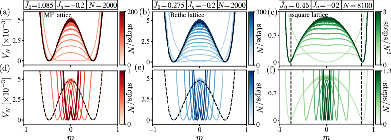
Figure S1: Equilibration and quench dynamics of the rate function. From left to right we show results for the MF lattice (red), Bethe lattice (blue), and square lattice (green). (a-c) Temporal evolution of $V_{N}(m;\tilde{J},t)$ as a function of $m$ during the equilibration round. (d-f) Temporal evolution of $V_{N}(m;\tilde{J},t)$ as a function of $m$ during the quench round. Different colors correspond to different times with increasing values from light to dark. Black dashed lines in (a-b, d-e) denote the theoretical equilibrium free energy density for the MF and Bethe lattice, respectively. Vertical black dashed lines in (c, f) correspond to Onsager’s spontaneous magnetization given by Eq. (S2).

S1.5 Curvature of the rate function and proxy for the critical time

To evaluate the curvature of the rate function $V_{N}^{\prime\prime}(m;\tilde{J},t)$ used for Fig. 1c,d in the Letter we used the finite difference method. Since the rate function contains strong fluctuations on the level of single spins with resolution $\Delta m=2/N$, we first coarse-grain the rate function through a binning procedure. For a bin size given by $2n+1\in\{1,3,..,\}$ we obtain a coarse-grained rate function in the following way

$$\hat{V}_{N,n}(m;\tilde{J},t)=-N^{-1}\ln{\left(\frac{1}{2n+1}\sum_{k=-n}^{n}P_{N}(m+2k/N;\tilde{J},t)\right)},\ {\rm for}\ m\in\{-(N+2n)/N,...,(N-2n)/N\}.$$ (S3)

Note that the factor $1/(2n+1)$ inside Eq. (S3) keeps the coarse-grained probability density normalized. After coarse-graining we obtain the curvature with the higher-order finite-difference method

$$\hat{V}_{N,n}^{\prime\prime}(m;\tilde{J},t)\approx\frac{\sum_{\eta=\pm}[-\hat{V}_{N,n}(m+4\eta/N;\tilde{J},t)+16\hat{V}_{N,n}(m+2\eta/N;\tilde{J},t)-15\hat{V}_{N,n}(m;\tilde{J},t)]}{12(2n/N)^{2}}+\mathcal{O}((2n/N)^{4}).$$ (S4)

In Fig. S2a-c we show the curvature around $m=0$ as a function of time $[{\rm steps}/N]$ for the MF lattice (a), Bethe lattice (b), and square lattice (c). In each of the lattices we find that the curvature quickly drops to a large negative value at a finite time. Interpreting the minima as a proxy for the critical time for finite systems attained at $t_{\rm min}$, we show in Fig. S2d-f that on the Bethe and square lattice this proxy is non-monotonic in $\tilde{J}_{q}$ for antiferromagnetic quenches. Furthermore, for the MF lattice the critical time decreases steadily with stronger antiferromagnetic quenches. Comparing these results with Fig. 2b in the Letter we find strong qualitative agreement between the results for $t_{c}$ obtained with theory and the proxy $t_{\rm min}$ obtained with kinetic MC simulations.

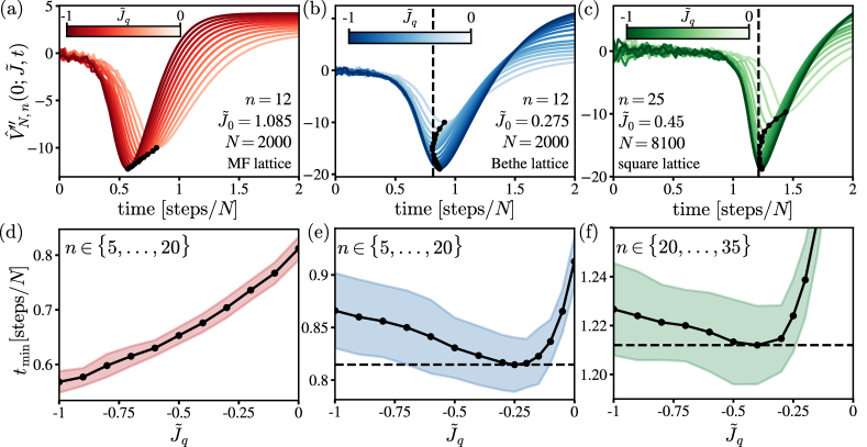
Figure S2: Curvature of the rate function around $\mathbf{m=0}$ and proxy for the critical time. From left to right we show results for the MF lattice (red), Bethe lattice (blue), and square lattice (green). (a-c) Temporal evolution of $V_{N,n}^{\prime\prime}(0;\tilde{J},t)$ (see Eq. (S3)) as a function of time $[{\rm steps}/N]$. Different colors correspond to different $\tilde{J}_{q}$ with increasing values from light to dark. Black dots indicate the minimum of the curvature, which we denote by $t_{\rm min}$ and take as a proxy for the critical time of the finite-time dynamical phase transition. Black dashed lines in (b-c) denote the minimum of $t_{\rm min}$ for the Bethe and square lattice, respectively. (d-f) Black line: Averaged critical time over various bin sizes $n$ (see range of $n$ in figure) as a function of $\tilde{J}_{q}$. Colored shaded area: Standard deviation of the critical time over various bin sizes $n$. Black dashed lines in (e-f) denote the minimum of $t_{\rm min}$ for the Bethe and square lattice, respectively.

S1.6 Evaluation of the relaxation time

To obtain the relaxation time $\tau_{r}$ from MC simulations we use the result for the relative entropy given by Eq. (9) in the Letter, i.e.

$$\mathscrsfs{D}_{t}{=}\lim_{N\rightarrow\infty}{\int_{-1}^{1}}\!\!\!\mathrm{e}^{-NV(m;\tilde{J}_{q},t)}[V_{\rm eq}(m;\tilde{J}_{q}){-}V(m;\tilde{J}_{q},t)]dm\simeq\sum_{k=2}^{\infty}\gamma_{k}(\tilde{J}_{0},\tilde{J}_{q})\mathrm{e}^{-kt/\tau_{r}(\tilde{J}_{q})}.$$ (S5)

Replacing the integral over $m$ in Eq. (S5) by a sum, we compute the relative entropy with the rate functions obtained from the MC simulations. To extract the relaxation time $\tau_{r}$ we make use of the exponential series on the right hand side of Eq. (S5) and take the long-time limit, which gives

$$\lim_{t\rightarrow\infty}\frac{\ln{(\mathscrsfs{D}_{t})}}{t}=\lim_{t\rightarrow\infty}\frac{\ln{(\gamma_{2}(\tilde{J}_{0},\tilde{J}_{q})\mathrm{e}^{-2t/\tau_{r}(\tilde{J}_{q})})}}{t}=-\frac{2}{\tau_{r}}.$$ (S6)

Plugging $\mathscrsfs{D}_{t}$ inferred from simulations into Eq. (S6) we extract the relaxation time as shown in Fig. 2e in the Letter.

S2 Hamiltonian formalism of large deviation function

Recall that $V(m;\tilde{J},t)\equiv\lim^{m={\rm const.}}_{N\rightarrow\infty}V_{N}(m;\tilde{J},t)$. In the SM of Meibohm and Esposito (2022a) it is shown that the rate function $V(m;\tilde{J}_{q},t)$ with quench temperature $\tilde{J}_{q}$ obeys the Hamilton-Jacobi (HJ) equation given by Eq. (5) in the Letter. The HJ equation can be solved with the method of characteristics as follows: Let $\{q(s),p(s)\}\ 0\leq s\leq t$ be the characteristics that solve the Hamilton’s equations

$$\dot{q}(s)=\partial_{p}\mathcal{H}(q,p),\ \dot{p}(s)=-\partial_{q}\mathcal{H}(q,p),\ q(t)=m,\ p(0)=\tilde{\rm f}^{\prime}(q(0);\tilde{J}_{0}),$$ (S7)

where $\dot{q}(s)\equiv dq(s)/ds$, $\dot{p}(s)\equiv dp(s)/ds$, $\tilde{\rm f}^{\prime}(a;\tilde{J})\equiv\partial_{m}\tilde{\rm f}(m;\tilde{J})|_{m=a}$, and $\mathcal{H}(q,p)$ is given by Eq. (6) in the Letter. Upon solving the Hamilton’s equations, the solution to the HJ equation reads

$$V(m;\tilde{J}_{q},t)=\int_{0}^{t}[p(s)\dot{q}(s)-\mathcal{H}(q,p)]ds+V(q(0);\tilde{J}_{0},0).$$ (S8)

For $t>t_{c}$, where $t_{c}=t_{c}(\tilde{J}_{0},\tilde{J}_{q})$ denotes the critical time, the solutions to the Hamilton’s equations become degenerate. Under these circumstances, the solution that minimizes Eq. (S8) corresponds to the stable solution Meibohm and Esposito (2022b).

S3 Lagrangian formalism of large deviation function

One can also obtain the solution to the HJ equation with the Lagrangian formalism, which is formally introduced in Külske and Le Ny (2007); Ermolaev and Külske (2010). The Lagrangian is obtained from the Hamiltonian via the backward Legendre transform $\mathcal{L}(q,\dot{q})=p(q,\dot{q})\dot{q}-\mathcal{H}(q,p(q,\dot{q}))$, where $p(q,\dot{q})$ can be obtained from the first of the Hamilton’s equations in Eq. (S7) and reads

$$p(q,\dot{q})=\frac{1}{2}\ln{\left(\frac{\dot{q}+\Lambda(q,\dot{q})}{4w^{+}(q;\tilde{J}_{q})}\right)},$$ (S9)

with $\Lambda(q,\dot{q})\equiv[16w^{+}(q;\tilde{J}_{q})w^{-}(q;\tilde{J}_{q})+\dot{q}^{2}]^{1/2}$. Plugging this expression back into $\mathcal{H}(q,p(q,\dot{q}))$ we obtain the Lagrangian

$$\mathcal{L}(q,\dot{q})=p(q,\dot{q})\dot{q}-\Lambda(q,\dot{q})/2+w^{+}(q;\tilde{J}_{q})+w^{-}(q;\tilde{J}_{q}).$$ (S10)

The Hamilton’s equations are replaced by the Euler-Lagrange (EL) equation, which reads

$$\ddot{q}(s)=2\Lambda(q,\dot{q})\partial_{q}[w^{+}(q;\tilde{J}_{q}){+}w^{-}(q;\tilde{J}_{q})]{-}8\partial_{q}w^{+}(q;\tilde{J}_{q})w^{-}(q;\tilde{J}_{q}),\ \dot{q}(0)=g(q(0)),\ q(t)=m.$$ (S11)

The boundary condition for $\dot{q}(0)$ is determined by the curve of allowed initial configurations (see also Eq. (24) in Ermolaev and Külske (2010))

$$g(m)\equiv 2\exp{(2\tilde{\rm f}^{\prime}(m;\tilde{J}_{0}))}w^{+}(m;\tilde{J}_{q})-2\exp{(-2\tilde{\rm f}^{\prime}(m;\tilde{J}_{0}))}w^{-}(m;\tilde{J}_{q}),$$ (S12)

which will be used in Sec. S4.2 to determine the symmetry-breaking transition. Upon solving the EL equation, the solution of the HJ equation is given by

$$V(m;\tilde{J}_{q},t)=\int_{0}^{t}\mathcal{L}(q(s),\dot{q}(s))ds+V(q(0);\tilde{J}_{0},0),$$ (S13)

which is identical to Eq. (S8). Similar to the Hamiltonian formalism, the solution of Eq. (S11) becomes degenerate for $t>t_{c}$. The stable solution for $q(s)$ minimizes the rate function given by Eq. (S13).

S4 Derivation of the critical time

In this section we derive the critical time $t_{c}$ based on two different approaches which are discussed in Meibohm and Esposito (2022a) and Ermolaev and Külske (2010), respectively. The first approach uses the Hamiltonian formalism discussed in Sec. S2 to derive an equation for the curvature at $m=0$. The second approach uses an invariance principle for the solutions of Eq. (S11) discussed in Sec. S3. Both approaches lead to the same result for the critical time given by Eq. (7) in the Letter. However, with the latter approach we can also derive the initial temperature below which the initial location of the cusp deviates from $m=0$.

S4.1 Hamiltonian formalism and the Ricatti equation

The critical time $t_{c}(\tilde{J}_{0},\tilde{J}_{q})$ is defined as the moment when the rate function $V(m;\tilde{J}_{q},t)$ develops a cusp at $m=0$, leading to a negatively diverging curvature. In the SM of Meibohm and Esposito (2022a) an equation for the curvature $V_{0}^{\prime\prime}(\tilde{J}_{q},t)\equiv V^{\prime\prime}(0;\tilde{J}_{q},t)$ is derived from the Hamilton’s equations. The resulting equation – after simplification – reads

$$\frac{dV^{\prime\prime}_{0}(\tilde{J}_{q},t)}{dt}=8w^{\pm}(0;\tilde{J}_{q})V^{\prime\prime}_{0}(\tilde{J}_{q},t)(\tilde{\rm f}^{\prime\prime}(0;\tilde{J}_{q})-V_{0}^{\prime\prime}(\tilde{J}_{q},t)),$$ (S14)

with initial condition $V_{0}^{\prime\prime}(\tilde{J}_{q},0)=\tilde{\rm f}^{\prime\prime}(0;\tilde{J}_{0})$. To obtain Eq. (S14) we explicitly used the detailed-balance relation $\ln{(w^{-}(m;\tilde{J})/w^{+}(m;\tilde{J}))}{=}2\tilde{\rm f}^{\prime}(m;\tilde{J})$ and the parity symmetry $w^{\pm}(m;\tilde{J}){=}w^{\mp}(-m;\tilde{J})$ to write $\partial_{m}w^{\pm}(m;\tilde{J})|_{m=0}=\mp w^{\pm}(0;\tilde{J})\tilde{\rm f}^{\prime\prime}(0;\tilde{J})$. Eq. (S14) is a so-called Ricatti equation, which can be solved analytically. The resulting solution up to the critical time reads

$$V^{\prime\prime}_{0}(\tilde{J}_{q},t)=\frac{\tilde{\rm f}^{\prime\prime}(0;\tilde{J}_{q})}{1-(1-\tilde{\rm f}^{\prime\prime}(0;\tilde{J}_{q})/\tilde{\rm f}^{\prime\prime}(0;\tilde{J}_{0}))\mathrm{e}^{-2t/\hat{\tau}_{r}(\tilde{J}_{q})}},$$ (S15)

where $1/\hat{\tau}_{r}(\tilde{J}_{q})\equiv 4w^{\pm}(0;\tilde{J}_{q})\tilde{\rm f}^{\prime\prime}(0;\tilde{J}_{q})$ is an effective relaxation rate. The critical time $t_{c}$ determines the root of the denominator in Eq. (S15). Solving for the root leads to Eq. (7) in the main Letter.

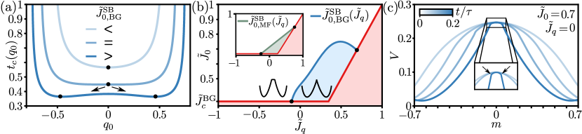
Figure S3: Symmetry-breaking transition for the location of the cusp. In all panels we consider a lattice with $\bar{z}=4$. (a) BG critical time $t^{\rm BG}_{c}(q_{0})$ given by Eq. (S19) as a function of the initial point $q_{0}$ for various values of the initial temperature $\tilde{J}_{0}$. The black dots indicate the minima of $t^{\rm BG}_{c}(q_{0})$, which set the location of the cusp. For $\tilde{J}_{0}>\tilde{J}^{\rm SB}_{\rm 0,BG}$ the critical time contains two minima $\pm q_{\rm min}$ (black dots), which correspond to non-zero cusp locations. (b) Blue line: BG symmetry-breaking temperature $\tilde{J}^{\rm SB}_{0}(\tilde{J}_{q})$ given by Eq. (S22) as a function of the quench temperature $\tilde{J}_{q}$. Inside the light blue region the cusp is formed at $m=0$, and in the white region the cusp is formed at $m\neq 0$. The red area is forbidden since $\tilde{J}_{0}>\tilde{J}^{\rm BG}_{c}$ and $\tilde{J}_{q}<\tilde{J}_{0}$. Inset: MF symmetry-breaking temperature $\tilde{J}^{\rm MF}_{0}(\tilde{J}_{q})$ given by Eq. (S21). Inside the light green region the cusp is formed at $m=0$. (c) Temporal evolution of the BG rate function $V_{\rm BG}(m;\tilde{J}_{q},t)$ for a quench to $\tilde{J}_{q}=0$. Time increases from light to dark blue. The initial temperature is set below the symmetry-breaking temperature, i.e. $\tilde{J}_{0}>\tilde{J}^{\rm SB}_{0}(\tilde{J}_{q})$, to induce a cusp at $m\neq 0$. Inset: Enlargement of the rate function around the center. Black arrows indicate the location of the cusps.

S4.2 Lagrangian formalism and the symmetry-breaking transition

Following the steps in Sec. 3.5 of Ermolaev and Külske (2010) we can derive the critical temperature $\tilde{J}^{\rm SB}_{0}(\tilde{J}_{q})$, below which the initial location of the cusp deviates from $\bar{m}=0$. The idea behind this calculation is that at the critical time the solution of Eq. (S11) converges to the same point $q(t_{c})$ for different initial conditions $\{q(0),\dot{q}(0)\}$. In other words, the location of $q(t_{c})$ remains invariant under a variation of the initial conditions. To determine the symmetry-breaking transition it suffices to consider the dynamics of $q(s)$ around the origin Ermolaev and Külske (2010). We linearize Eq. (S11) around the point $(q,\dot{q})=(0,0)$, which yields

$$\ddot{q}(s) = q(s)/\hat{\tau}_{r}^{2}(\tilde{J}_{q}),\ \dot{q}(0)=g(q_{0})\equiv v_{0},\ q(0)\equiv q_{0},$$ (S16)

where $\{q_{0},v_{0}(q_{0})\}$ are the initial conditions, and $1/\hat{\tau}_{r}(\tilde{J}_{q})\equiv 4w^{\pm}(0;\tilde{J}_{q})\tilde{\rm f}^{\prime\prime}(0;\tilde{J}_{q})$. The solution of Eq. (S16) is given by

$$q(s)=(q_{0}/2-\hat{\tau}_{r}v_{0}/2)\mathrm{e}^{-s/\hat{\tau}_{r}}+(q_{0}/2+\hat{\tau}_{r}v_{0}/2)\mathrm{e}^{s/\hat{\tau}_{r}}.$$ (S17)

We now consider a variation of $q(s)$ w.r.t. the initial conditions $\{q_{0},v_{0}(q_{0})\}$, which gives

$$\frac{dq(s)}{dq_{0}}=\frac{\partial q(s)}{\partial q_{0}}+\frac{\partial q(s)}{\partial v_{0}}g^{\prime}(q_{0})=(1/2-\hat{\tau}_{r}g^{\prime}(q_{0})/2)\mathrm{e}^{-s/2\hat{\tau}_{r}}+(1/2+\hat{\tau}_{r}g^{\prime}(q_{0})/2)\mathrm{e}^{s/2\hat{\tau}_{r}},$$ (S18)

where $g^{\prime}(q_{0})\equiv dg(m)/dm|_{m=q_{0}}$ and $g(m)$ is given by Eq. (S12). At the critical time $s=t_{c}$ the variation (S18) vanishes, which leads to the critical time in the form

$$t_{c}(q_{0})=(\hat{\tau}_{r}/2)\ln{\left(\frac{g^{\prime}(q_{0})-1/\hat{\tau}_{r}}{g^{\prime}(q_{0})+1/\hat{\tau}_{r}}\right)}.$$ (S19)

For $\tilde{J}_{c}<\tilde{J}_{0}<\tilde{J}^{\rm SB}_{0}(\tilde{J}_{q})$ the critical time given by Eq. (S19) has a single minimum at $q_{\rm min}=0$ (see upper line in Fig. S3a). Inserting $q_{0}=0$ and recalling the relation $\partial_{m}w^{\pm}(m;\tilde{J})|_{m=0}=\mp w^{\pm}(0;\tilde{J})\tilde{\rm f}^{\prime\prime}(0;\tilde{J})$ we obtain the critical time given by Eq. (7) in the Letter.

For $\tilde{J}_{0}>\tilde{J}^{\rm SB}_{0}(\tilde{J}_{q})$ Eq. (S19) develops two minima at $\pm q_{\rm min}\neq 0$, corresponding to the new cusp locations (see lower line in Fig. S3a).

For $\tilde{J}_{0}=\tilde{J}^{\rm SB}_{0}(\tilde{J}_{q})$ the curvature of Eq. (S19) at $q_{0}=0$ vanishes (see middle line in Fig. S3a), which results in the following equation determining $\tilde{J}^{\rm SB}_{0}(\tilde{J}_{q})$

$$g^{\prime\prime\prime}(0)|_{\tilde{J}^{\rm SB}_{0}(\tilde{J}_{q})}=0,$$ (S20)

where we have used that $g^{\prime\prime}(0)=0$. Solving Eq. (S20) for the MF approximation we obtain the simple result

$$\tilde{J}^{\rm SB}_{0,{\rm MF}}(\tilde{J}_{q})=\frac{3+\bar{z}\tilde{J}_{q}}{2\bar{z}}.$$ (S21)

For $\tilde{J}_{q}=0$ we obtain $\tilde{J}^{\rm SB}_{0,{\rm MF}}(0)=3/2z$ as mentioned in Külske and Le Ny (2007); Ermolaev and Külske (2010). For the BG approximation the general formula for $\tilde{J}^{\rm SB}_{0,{\rm BG}}(\tilde{J}_{q})$ is rather long and therefore not shown. For $\bar{z}=4$ the result can compactly be written as

$$\tilde{J}^{\rm SB}_{0,{\rm BG}}(\tilde{J}_{q})|_{z=4}=\ln{(x_{\tilde{J}_{q}})}/2,$$ (S22)

where $x_{\tilde{J}_{q}}$ is the real solution of the following cubic equation

$$20{-}16(1{+}2\mathrm{e}^{-2\tilde{J}_{q}})x_{\tilde{J}_{q}}{+}(8{+}8\mathrm{e}^{-2\tilde{J}_{q}}{+}20\mathrm{e}^{-4\tilde{J}_{q}})x_{\tilde{J}_{q}}^{2}{-}(2{-}4\mathrm{e}^{-2\tilde{J}_{q}}{+}10\mathrm{e}^{-4\tilde{J}_{q}}{-}\mathrm{e}^{-8\tilde{J}_{q}}{+}6\mathrm{e}^{-10\tilde{J}_{q}}{-}9\mathrm{e}^{-12\tilde{J}_{q}}{+}4\mathrm{e}^{-14\tilde{J}_{q}})x_{\tilde{J}_{q}}^{3}{=}0.$$ (S23)

For $\tilde{J}_{q}=0$ we obtain $\tilde{J}^{\rm SB}_{0,{\rm BG}}(0)=\ln{(\frac{\bar{z}+1}{\bar{z}-2})}/2$ as mentioned in the Letter. In Fig. S3b we plot Eq. (S22) as a function of $\tilde{J}_{0}$ with the dark blue line. Interestingly, the light blue region for which the cusp appears at $m=0$ is rather small and of finite area. Correspondingly, in Fig. S3c we provide an example of the rate function $V_{\rm BG}(m;\tilde{J}_{q},t)$ for which the cusps appear at a non-zero locations.

S5 Bounds on the BG critical time

In this section we derive the bounds for the BG critical time $t^{\rm BG}_{c}$. Inserting the BG free energy density and transition rates – given by Eqs. (2) and (4) in the Letter – into Eq. (7) in the Letter, we obtain

$$t^{\rm BG}_{c}(\tilde{J}_{0},\tilde{J}_{q})=\frac{\cosh^{\bar{z}}{(\tilde{J}_{q})}(\tanh{(\tilde{J}_{q})}+1)}{4((\bar{z}-1)\tanh{(\tilde{J}_{q})}-1)}\left[\tilde{J}_{q}+\ln{\left(\frac{(\bar{z}-1)\sinh{(\tilde{J}_{0})}-\cosh{(\tilde{J}_{0})}}{\bar{z}\sinh{(\tilde{J}_{0}-\tilde{J}_{q})}}\right)}\right],$$ (S24)

where $\tilde{J}_{0}>\tilde{J}^{\rm BG}_{c}\equiv\ln{(\bar{z}/(\bar{z}-2))}/2$ and $\tilde{J}_{q}\leq\tilde{J}_{0}$. Fig. 2b in the Letter displays the BG critical given by Eq. (S24) with the green line. The BG critical time has a minimum for an anti-ferromagnetic quench $\tilde{J}_{q}<0$, which cannot be determined analytically. We can, however, derive lower bounds on the critical time. To construct the bounds we will distinguish between quenches in the one- and two-phase domain, i.e. $\tilde{J}_{q}<\tilde{J}^{\rm BG}_{c}$ and $\tilde{J}_{q}\geq\tilde{J}^{\rm BG}_{c}$. The general result for the anti-ferromagnetic bound is given by Eq. (8) in the Letter.

S5.1 $\tilde{J}_{q}<\tilde{J}^{\rm BG}_{c}$

For quenches in the one-phase domain we can bound the critical time by applying the well-known inequality $\ln{(1+x)}>2x/(2+x)$ for $x>0$ Love (1980) to the logarithmic term in Eq. (7) in the Letter (since $-\tilde{\rm f}_{\rm BG}^{\prime\prime}(0;\tilde{J}_{q})/\tilde{\rm f}_{\rm BG}^{\prime\prime}(0;\tilde{J}_{0})>0$). This yields the local lower bound

$$t^{\dagger{\rm BG}}_{c}(\tilde{J}_{0},\tilde{J}_{q})=\frac{\cosh^{\bar{z}}{(\tilde{J}_{q})}}{\bar{z}-2+\bar{z}\mathrm{e}^{-2\tilde{J}_{q}}-2\bar{z}\mathrm{e}^{-2\tilde{J}_{0}}}.$$ (S25)

In Fig. S4a we plot $t^{\dagger{\rm BG}}_{c}$ with the black line. Surprisingly, this local bound also seems to work for $\tilde{J}_{q}\geq\tilde{J}^{\rm BG}_{c}$, even though $-\tilde{\rm f}_{\rm BG}^{\prime\prime}(0;\tilde{J}_{q})/\tilde{\rm f}_{\rm BG}^{\prime\prime}(0;\tilde{J}_{0})<0$. Furthermore, it gives the exact result for $\tilde{J}_{q}=\tilde{J}^{\rm BG}_{c}$ given by Eq. (S32). The lower bound is also non-monotonic w.r.t. $\tilde{J}_{q}$, and displays a minimum for an anti-ferromagnetic quench $\tilde{J}_{q}<0$ which we show in the next section. At the respective minimum, the global lower bound $\inf_{\tilde{J}_{q}}t^{\dagger{\rm BG}}_{c}(\tilde{J}_{0},\tilde{J}_{q})$ (see black dashed line in Fig. S4a) is given by Eq. (8) in the Letter. Taking the limit $\tilde{J}_{0}\rightarrow\infty$ of Eq. (8), we further obtain the following universal global lower bound independent of $\tilde{J}_{q}$ and $\tilde{J}_{0}$ that reads

$$\lim\limits_{\tilde{J}_{0}\rightarrow\infty}\inf_{\tilde{J}_{q}}t^{\dagger{\rm BG}}_{c}(\tilde{J}_{0},\tilde{J}_{q})=\frac{(\bar{z}-2)^{1-\bar{z}/2}[2+\nu_{\bar{z}}]^{-\bar{z}/2}[\bar{z}+\nu_{\bar{z}}]^{\bar{z}}}{2^{\bar{z}}(4+\bar{z}[\bar{z}-2+\nu_{\bar{z}}])},$$ (S26)

with $\nu_{\bar{z}}\equiv\sqrt{8+\bar{z}(\bar{z}-4)}$. For $\bar{z}=4$ this gives the universal global lower bound $t^{\dagger{\rm BG}}_{c}(\tilde{J}_{0},\tilde{J}_{q})>1/8$ and is shown with the red line in Fig. S4a. In Fig. S4b we observe that for increasing $\bar{z}$ the bounds given by Eq. (8) in the Letter and Eq. (S26) become sharper with respect to the true/exact minimum of $t^{\rm BG}_{c}$.

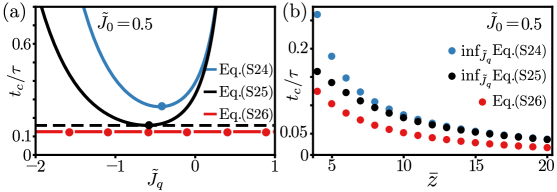
Figure S4: Bounds on the BG critical time for quenches in the one-phase domain. (a) BG critical time $t^{\rm BG}_{c}(\tilde{J}_{0},\tilde{J}_{q})$ given by Eq. (S24) (blue line) as a function of the quench temperature $\tilde{J}_{q}$ for $\tilde{J}_{0}=0.5$ and $\bar{z}=4$. The respective lower bounds are shown with the black and red line. (b) Minimum of the BG critical time (blue dots) as a function of the lattice coordination number $\bar{z}$. The respective lower bounds are shown with the black and red dots, respectively.

S5.1.1 Proof that the minimum is attained at an antiferromagnetic coupling

It is to show that

$$\tilde{J}_{q}^{\dagger}(\tilde{J}_{0})\equiv\arg\min_{\tilde{J}_{q}}t^{\dagger}_{c}(\tilde{J}_{0},\tilde{J}_{q})=\frac{1}{2}\ln\left(\frac{\bar{z}-2}{\bar{z}{\rm e}^{-2\tilde{J}_{0}}\!+\!2\!+\Delta_{\bar{z}}(\tilde{J}_{0})}\right)\leq 0$$ (S27)

with $\Delta_{\bar{z}}(\tilde{J}_{0})\equiv[8{+}\bar{z}^{2}\mathrm{e}^{-4\tilde{J}_{0}}{+}\bar{z}(\bar{z}{-}4)(1{-}2\mathrm{e}^{-2\tilde{J}_{0}})]^{\frac{1}{2}}$ for $\tilde{J}_{0}\geq\tilde{J}^{\rm BG}_{c}\equiv\ln{(\bar{z}/(\bar{z}-2))}/2$. Since

$$\lim_{\tilde{J}_{0}\to\infty}\tilde{J}_{q}^{\dagger}(\tilde{J}_{0})=\frac{1}{2}\ln{\left(\frac{\bar{z}-2}{2+\sqrt{\bar{z}^{2}-4\bar{z}+8}}\right)}\leq\frac{1}{2}\ln{\left(\frac{\bar{z}-2}{\sqrt{\bar{z}^{2}-4\bar{z}+4}}\right)}=0,$$ (S28)

and because $\tilde{J}_{q}^{\dagger}(\tilde{J}_{0})$ is a continuously differentiable function of $\tilde{J}_{0}$ for $\tilde{J}_{0}\geq\tilde{J}^{\rm BG}_{c}$, it suffices to show that $d\tilde{J}_{q}^{\dagger}(\tilde{J}_{0})/d\tilde{J}_{0}\geq 0$ for $\tilde{J}_{0}\geq\tilde{J}^{\rm BG}_{c}$. To that aim let us differentiate Eq. (S27) w.r.t. $\tilde{J}_{0}$:

$$\frac{d\tilde{J}_{q}^{\dagger}}{d\tilde{J}_{0}}=-\frac{1}{2}\frac{-2\bar{z}\mathrm{e}^{-2\tilde{J}_{0}}+\Delta^{\prime}_{\bar{z}}(\tilde{J}_{0})}{\bar{z}\mathrm{e}^{-2\tilde{J}_{0}}+2+\Delta_{\bar{z}}(\tilde{J}_{0})}.$$ (S29)

Noting that $\bar{z}\mathrm{e}^{-2\tilde{J}_{0}}+2+\Delta_{\bar{z}}(\tilde{J}_{0})>0$ for all $\tilde{J}_{0}\geq\tilde{J}^{\rm BG}_{c}$, it remains to be shown that $-2\bar{z}\mathrm{e}^{-2\tilde{J}_{0}}+\Delta^{\prime}_{\bar{z}}(\tilde{J}_{0})\leq 0$. Evaluating the derivative of $\Delta_{\bar{z}}(\tilde{J}_{0})$ we find

$$\Delta^{\prime}_{\bar{z}}(\tilde{J}_{0})=\frac{2\bar{z}(\bar{z}-4)\mathrm{e}^{-2\tilde{J}_{0}}-2\bar{z}^{2}\mathrm{e}^{-4\tilde{J}_{0}}}{\sqrt{8{+}\bar{z}^{2}\mathrm{e}^{-4\tilde{J}_{0}}{+}\bar{z}(\bar{z}{-}4)(1{-}2\mathrm{e}^{-2\tilde{J}_{0}})}},$$ (S30)

which means that to prove $d\tilde{J}_{q}^{\dagger}(\tilde{J}_{0})/d\tilde{J}_{0}\geq 0$ for $\tilde{J}_{0}\geq\tilde{J}^{\rm BG}_{c}$ we must only show that

$$\frac{\bar{z}-4-\bar{z}\mathrm{e}^{-2\tilde{J}_{0}}}{\sqrt{8{+}\bar{z}^{2}\mathrm{e}^{-4\tilde{J}_{0}}{+}\bar{z}(\bar{z}{-}4)(1{-}2\mathrm{e}^{-2\tilde{J}_{0}})}}\leq 1\implies(\bar{z}-4-\bar{z}\mathrm{e}^{-2\tilde{J}_{0}})^{2}\leq 8{+}\bar{z}^{2}\mathrm{e}^{-4\tilde{J}_{0}}{+}\bar{z}(\bar{z}{-}4)(1{-}2\mathrm{e}^{-2\tilde{J}_{0}}).$$ (S31)

Writing out the right hand side and canceling terms which are on both sides we finally obtain $4(2-\bar{z})\leq 0$, which is indeed the case for $\bar{z}\geq 2$. Hence, since we have shown that $J_{q}^{\dagger}(\tilde{J}_{0})$ is monotonically increasing for $\tilde{J}_{0}\geq\tilde{J}^{\rm BG}_{c}$, and since $\lim_{\tilde{J}_{0}\to\infty}\tilde{J}_{q}^{\dagger}(\tilde{J}_{0})<0$, the lower bound in Eq. (S27) follows immediately.

S5.2 $\tilde{J}_{q}\geq\tilde{J}^{\rm BG}_{c}$

For quenches in the two-phase domain we prove that the BG critical time $t^{\rm BG}_{c}(\tilde{J}_{0},\tilde{J}_{q})$ is bounded from below by the critical quench $t^{\rm BG}_{c}(\tilde{J}_{0},\tilde{J}^{\rm BG}_{c})$, which reads

$$t^{\rm BG}_{c}(\tilde{J}_{0},\tilde{J}^{\rm BG}_{c})=\left(\frac{\bar{z}-1}{\sqrt{\bar{z}(\bar{z}-2)}}\right)^{\bar{z}}\frac{\tanh{(\tilde{J}_{0})}+1}{4((\bar{z}-1)\tanh{(\tilde{J}_{0})}-1)}.$$ (S32)

To prove that Eq. (S32) provides a lower bound for the critical time for quenches in the two-phase domain, we first differentiate Eq. (S24) w.r.t. $\tilde{J}_{q}$, which gives

$$\frac{\partial t^{\rm BG}_{c}(\tilde{J}_{0},\tilde{J}_{q})}{\partial\tilde{J}_{q}}=\frac{\bar{z}(1+\tanh{(\tilde{J}_{q})})\cosh^{\bar{z}}{(\tilde{J}_{q})}}{4((\bar{z}-1)\tanh{(\tilde{J}_{q})}-1)^{2}}\mathcal{A}_{1}(\tilde{J}_{0},\tilde{J}_{q}),$$ (S33)

where we have introduced the auxiliary function (and subsequent auxiliary functions)

$$\mathcal{A}_{1}(\tilde{J}_{0},\tilde{J}_{q}) \equiv -\mathcal{A}_{2}(\tilde{J}_{0},\tilde{J}_{q})[1-\tanh{(\tilde{J}_{q})}]-\mathcal{A}_{3}(\tilde{J}_{q})\ln{(\mathcal{A}_{2}(\tilde{J}_{q},\tilde{J}_{0}))},$$

$$\mathcal{A}_{2}(\tilde{J}_{0},\tilde{J}_{q}) \equiv [(\bar{z}{-}1)\tanh{(\tilde{J}_{q})}{-}1][1+\tanh{(\tilde{J}_{0})}]/[\bar{z}(\tanh{(\tilde{J}_{q})}-\tanh{(\tilde{J}_{0})})],$$

$$\mathcal{A}_{3}(\tilde{J}_{q}) \equiv 1{-}(\bar{z}{-}1)\tanh^{2}{(\tilde{J}_{q})}.$$ (S34)

All terms in front of $\mathcal{A}_{1}(\tilde{J}_{0},\tilde{J}_{q})$ in Eq. (S33) are trivially positive. If furthermore $\mathcal{A}_{1}(\tilde{J}_{0},\tilde{J}_{q})>0$ for $\tilde{J}^{\rm BG}_{c}<\tilde{J}_{q}<\tilde{J}_{0}$, then we know that Eq. (S32) provides a lower bound. To prove that the latter is positive we proceed in two steps.

S5.2.1 $\mathcal{A}_{2}(\tilde{J}_{q},\tilde{J}_{0})>1\ \forall\tilde{J}_{q}>\tilde{J}^{\rm BG}_{c}$

First we focus on the term $\mathcal{A}_{2}(\tilde{J}_{q},\tilde{J}_{0})$ entering the logarithm in $\mathcal{A}_{1}(\tilde{J}_{0},\tilde{J}_{q})$. Here we prove that $\mathcal{A}_{2}(\tilde{J}_{q},\tilde{J}_{0})>1\ \forall\tilde{J}_{q}>\tilde{J}^{\rm BG}_{c}$, which we need for the second step. First, note that $\mathcal{A}_{2}(\tilde{J}^{\rm BG}_{c},\tilde{J}_{0})=1$, which can easily be checked by hand. Introducing $x_{0}\equiv\tanh{(\tilde{J}_{0})}$ and $x_{q}\equiv\tanh{(\tilde{J}_{q})}$, we find $\partial_{\tilde{J}_{q}}\mathcal{A}_{2}(\tilde{J}_{q},\tilde{J}_{0})=\cosh^{-2}(\tilde{J}_{q})\partial_{x_{q}}\mathcal{A}_{2}(x_{q},x_{0})>0\ \forall\tilde{J}_{0}>\tilde{J}^{\rm BG}_{c}$. To see this, we write out the partial derivative and obtain

$$\partial_{x_{q}}\mathcal{A}_{2}(x_{q},x_{0})=\partial_{x_{q}}\left(\frac{(1+x_{q})[(\bar{z}{-}1)x_{0}{-}1]}{\bar{z}(x_{0}-x_{q})}\right)=\frac{(1+x_{0})((\bar{z}-1)x_{0}-1)}{\bar{z}(x_{0}-x_{q})^{2}}>0\ \forall x_{0}>(\bar{z}-1)^{-1}.$$ (S35)

Finally, note that $x_{0}>(\bar{z}-1)^{-1}$ translates to $\tilde{J}_{0}>\operatorname{arctanh}{(\bar{z}-1)^{-1}}=\tilde{J}^{\rm BG}_{c}$, which is the regime of interest. Hence, $\mathcal{A}_{2}(\tilde{J}_{q},\tilde{J}_{0})$ has a positive slope w.r.t. $\tilde{J}_{q}$. Combined with $\mathcal{A}_{2}(\tilde{J}^{\rm BG}_{c},\tilde{J}_{0})=1$, this proves that $\mathcal{A}_{2}(\tilde{J}_{q},\tilde{J}_{0})>1\ \forall\tilde{J}_{q}>\tilde{J}^{\rm BG}_{c}$.

S5.2.2 $\mathcal{A}_{1}(\tilde{J}_{0},\tilde{J}_{q})>0\ \forall\tilde{J}_{q}>\tilde{J}^{\rm BG}_{c}$

Now we turn our attention to $\mathcal{A}_{1}(\tilde{J}_{0},\tilde{J}_{q})$. We begin by considering the regime $\tanh(\tilde{J}_{q})\geq 1/\sqrt{z-1}$. Here $\mathcal{A}_{3}(\tilde{J}_{q})<0$, and therefore $-\mathcal{A}_{3}(\tilde{J}_{q})\ln{(\mathcal{A}_{2}(\tilde{J}_{q},\tilde{J}_{0}))}>0$ based on the previous step. Furthermore, $-\mathcal{A}_{2}(\tilde{J}_{0},\tilde{J}_{q})[1-\tanh{(\tilde{J}_{q})}]>0\ \forall\tilde{J}^{\rm BG}_{c}<\tilde{J}_{q}<\tilde{J}_{0}$, and so it follows that $\mathcal{A}_{1}(\tilde{J}_{0},\tilde{J}_{q})>0$ for $1/\sqrt{z-1}\leq\tanh{(\tilde{J}_{q}})\leq\tanh{(\tilde{J}_{0}})$.
Next we consider the regime $1/(z{-}1){<}\tanh(\tilde{J}_{q}){<}1/\sqrt{z{-}1}$. Here $\mathcal{A}_{3}(\tilde{J}_{q}){>}0$, and therefore ${-}\mathcal{A}_{3}(\tilde{J}_{q})\ln{(\mathcal{A}_{2}(\tilde{J}_{q},\tilde{J}_{0}))}{<}0$. To construct a bound for $\mathcal{A}_{1}(\tilde{J}_{0},\tilde{J}_{q})$ we apply the following chain of inequalities

$$\mathcal{A}_{1}(\tilde{J}_{0},\tilde{J}_{q}) \equiv \mathcal{A}_{3}(\tilde{J}_{q})[-\mathcal{A}_{2}(\tilde{J}_{0},\tilde{J}_{q})[1-\tanh{(\tilde{J}_{q})}]/\mathcal{A}_{3}(\tilde{J}_{q})-\ln{(\mathcal{A}_{2}(\tilde{J}_{q},\tilde{J}_{0}))}]$$

$$> \mathcal{A}_{3}(\tilde{J}_{q})[-\mathcal{A}_{2}(\tilde{J}_{0},\tilde{J}_{q})[1-\tanh{(\tilde{J}_{q})}]/\mathcal{A}_{3}(\tilde{J}_{q})-\mathcal{A}_{2}(\tilde{J}_{q},\tilde{J}_{0})+1]$$

$$> \mathcal{A}_{3}(\tilde{J}_{q})[-\mathcal{A}_{2}(\tilde{J}_{0},\tilde{J}_{q})-\mathcal{A}_{2}(\tilde{J}_{q},\tilde{J}_{0})+1]=0.$$

In passing from the first to the second line we have applied the inequality $\ln{(z)}<z-1$ for $z>1$. From the second to the third line we have used $[1-\tanh{(\tilde{J}_{q})}]/\mathcal{A}_{3}(\tilde{J}_{q})>1$ for $1/(z{-}1){<}\tanh(\tilde{J}_{q}){<}1/\sqrt{z{-}1}$. Finally, in the last line we used that $1-\mathcal{A}_{2}(x_{0},x_{q})-\mathcal{A}_{2}(x_{q},x_{0})=0$, which follows by simply writing out the terms.
Combining the results we find that $\mathcal{A}_{1}(\tilde{J}_{0},\tilde{J}_{q})>0$ for $\tilde{J}^{\rm BG}_{c}<\tilde{J}_{q}<\tilde{J}_{0}$, and therefore $t^{\rm BG}_{c}(\tilde{J}_{0},\tilde{J}_{q})$ is bounded by Eq. (S32) in this regime.

S6 Relaxation dynamics

In this section we focus on the relaxation dynamics of the minima of the rate function, $\bar{m}(t,\tilde{J}_{0},\tilde{J}_{q})\equiv\arg\min_{m}V(m;\tilde{J}_{q},t)$, which we need to evaluate the relative entropy in Sec. S7. Based on the first characteristic equation in Eq. (S7) we find that the minima obey the differential equation

$$\frac{d\bar{m}(t,\tilde{J}_{0},\tilde{J}_{q})}{dt}=2w^{+}(\bar{m};\tilde{J}_{q})-2w^{-}(\bar{m};\tilde{J}_{q}).$$ (S36)

As the right-hand side (RHS) does not depend explicitly on time, the solution is given by the integral

$$\frac{1}{2}\int\frac{d\bar{m}}{w^{+}(\bar{m};\tilde{J}_{q})-w^{-}(\bar{m};\tilde{J}_{q})}=t+\mathcal{C},$$ (S37)

where $\mathcal{C}=\mathcal{C}(\tilde{J}_{0},\tilde{J}_{q})$ is an integration constant left to be determined from the initial condition at $t=0$. The integral on the left-hand side (LHS) cannot be evaluated analytically upon inserting the MF transition rates (see Eq. (3) in Meibohm and Esposito (2022a) for their functional form). However, for the BG transition rates given by Eq. (4) in the Letter, the integral can be evaluated explicitly for $\bar{z}=\{2,3,4,5,6\}$. Here we show the analysis for $\bar{z}=\{2,4\}$, where we use the former as an educative introduction to carry out the latter. Our aim is to go beyond the linear response regime studied in Saito and Kubo (1976) by applying the so-called Lagrange Inversion Theorem.

S6.1 BG approximation with $\bar{z}=2$

Formally the mean magnetization for $\bar{z}=2$ vanishes for any initial and final temperature. However, instead of considering a temperature quench, we consider a magnetization quench where we initially prepare the system in a non-zero magnetic state with $\bar{m}(0)\equiv\bar{m}_{0}\neq 0$. Inserting the BG transition rates with $\bar{z}=2$ into Eq. (S37) we obtain – after some algebraic manipulation – the result

$$-\tau_{r}(\tilde{J}_{q})\ln{(\bar{m}/g(\bar{m};\tilde{J}_{q}))}=t+\mathcal{C},$$ (S38)

where $1/\tau_{r}(\tilde{J}_{q})\equiv 4w^{\pm}_{\rm BG}(0;\tilde{J}_{q})\tilde{\rm f}^{\prime\prime}_{\rm BG}(0;\tilde{J}_{q})=8/(1+\mathrm{e}^{2\tilde{J}_{q}})^{2}$ is the relaxation rate for $\bar{z}=2$, and we have introduced the auxiliary function

$$g(\bar{m};\tilde{J}_{q})\equiv\exp{(-\tanh{(\tilde{J}_{q})}\ln{(\alpha_{+})}-\alpha_{-}/(2\cosh{(\tilde{J}_{q})}\bar{m})^{2})},$$ (S39)

with

$$\alpha_{\pm}(\bar{m};\tilde{J}_{q})\equiv\exp{(2\tilde{J}_{q})}\pm[\bar{m}^{2}{+}\exp{(4\tilde{J}_{q})}(1{-}\bar{m}^{2})]^{1/2}.$$ (S40)

From Eq. (S38) we directly read off the integration constant $\mathcal{C}=\mathcal{C}(\bar{m}_{0},\tilde{J}_{q})$ at $t=0$. To obtain an explicit solution for $\bar{m}$ we multiply both sides of Eq. (S38) by $-\tau_{r}$, and subsequently exponentiate, resulting in

$$\frac{\bar{m}}{g(\bar{m};\tilde{J}_{q})}=\frac{\bar{m}_{0}}{g(\bar{m}_{0};\tilde{J}_{q})}\mathrm{e}^{-t/\tau_{r}(\tilde{J}_{q})},$$ (S41)

where we have now also fixed the integration constant. Now we invoke the Lagrange inversion theorem: Let $f(w)$ be analytic in some neighborhood of the point $w=0$ (of the complex plane) with $f(0)\neq 0$ and let it satisfy the equation

$$\frac{w}{f(w)}=\xi.$$ (S42)

Then $\exists a,b\in\mathbbm{R}^{+}$ such that for $|\xi|<a$ Eq. (S42) has only a single solution in the domain $|w|<b$. According to the Lagrange-Bürmann formula this unique solution is an analytical function of $\xi$ given by

$$w=\sum_{k=1}^{\infty}\frac{\xi^{k}}{k!}\left[\frac{d^{k-1}}{dw^{k-1}}f(w)^{k}\right]_{w=0}.$$ (S43)

Note that Eq. (S41) is similar in structure to Eq. (S42), and furthermore

$$g(0;\tilde{J}_{q})=\exp{(-\tanh{(\tilde{J}_{q})}(1/2{+}\ln{2}{+}2\tilde{J}_{q}))},$$ (S44)

which is non-zero $\forall\tilde{J}_{q}\in\mathbb{R}$. Therefore, we can use Eq. (S43) to obtain an explicit solution for $\bar{m}$, yielding

$$\bar{m}(t,\bar{m}_{0},\tilde{J}_{q})=\sum_{k=1}^{\infty}\frac{\bar{m}^{k}_{0}}{g(\bar{m}_{0};\tilde{J}_{q})^{k}k!}\left[\frac{d^{k-1}}{dw^{k-1}}g(\bar{m};\tilde{J}_{q})^{k}\right]_{\bar{m}=0}\mathrm{e}^{-kt/\tau_{r}(\tilde{J}_{q})}=\sum_{k=1}^{\infty}\alpha_{k}(\bar{m}_{0};\tilde{J}_{q})\mathrm{e}^{-kt/\tau_{r}(\tilde{J}_{q})}.$$ (S45)

For completeness, we list the first three non-zero coefficients

$$\alpha_{1}(\bar{m}_{0};\tilde{J}_{q}) = \bar{m}_{0}g(0;\tilde{J}_{q})/g(\bar{m}_{0};\tilde{J}_{q}),$$

$$\alpha_{3}(\bar{m}_{0};\tilde{J}_{q}) = \alpha^{3}_{1}(\bar{m}_{0};\tilde{J}_{q})\mathrm{e}^{-4\tilde{J}_{q}}(1-\mathrm{e}^{2\tilde{J}_{q}})^{2}/8,$$

$$\alpha_{5}(\bar{m}_{0};\tilde{J}_{q}) = \alpha^{5}_{1}(\bar{m}_{0};\tilde{J}_{q})\mathrm{e}^{-4\tilde{J}_{q}}\sinh{(\tilde{J}_{q})}^{3}(4\cosh{(\tilde{J}_{q})}+5\sinh{(\tilde{J}_{q})})/8.$$ (S46)

Note that $\alpha_{1}(\bar{m}_{0};0)=\bar{m}_{0}$ and $\alpha_{k}(\bar{m}_{0};0)=0\ \forall k\in\{2,3,...\}$, which gives the well-known result $\bar{m}(t,\bar{m}_{0},0)=\bar{m}_{0}\exp{(-2t)}$ Ermolaev and Külske (2010). Furthermore, since $g(\bar{m};\tilde{J}_{q})=g(-\bar{m};\tilde{J}_{q})$, we know that $\alpha_{2k}=0\ \forall k\in\mathbb{N}$. This concludes our derivation of $\bar{m}(t,\bar{m}_{0},\tilde{J}_{q})$ for $\bar{z}=2$.

S6.2 BG approximation with $\bar{z}=4$

Now we focus on the case $\bar{z}=4$. The analysis requires the same steps as shown in the previous section, but involves a bit more algebra. We will focus only on quenches where the initial temperature is below the critical temperature, i.e. $\tilde{J}_{0}>\tilde{J}^{\rm BG}_{c}=\ln{(2)}/2$, resulting in the following initial magnetization Blom and Godec (2021)

$$\bar{m}_{0}(\tilde{J}_{0})=\mathrm{e}^{2\tilde{J}_{0}}(\mathrm{e}^{4\tilde{J}_{0}}-4)^{1/2}/(\mathrm{e}^{4\tilde{J}_{0}}-2).$$ (S47)

In order to apply the Lagrange inversion theorem we have to make a distinction between quenches above and below the critical temperature, since they have different equilibrium states. Furthermore, for quenches above the critical temperature $\tilde{J}_{q}\leq\ln{(2)}/2$, we will encounter a particular “special” value $\tilde{J}_{q}=\ln{(2)}/4$ which needs to be handled separately.

S6.2.1 $\tilde{J}_{q}<\ln{(2)}/2$ and $\tilde{J}_{q}\neq\ln{(2)}/4$

Upon determining the integral in Eq. (S37) for $\bar{z}=4$ we obtain an analytic expression which can be written in a similar form as Eq. (S38). In this regime the relaxation rate is given by $1/\tau_{r}(\tilde{J}_{q})\equiv 4w^{\pm}_{\rm BG}(0;\tilde{J}_{q})\tilde{\rm f}^{\prime\prime}_{\rm BG}(0;\tilde{J}_{q})=\cosh^{4}{(\tilde{J}_{q})}/(4\exp{(-2\tilde{J})}-2)$, which is plotted in Fig. 2d in the Letter (green + blue line). The auxiliary function $g(\bar{m};\tilde{J}_{q})$ in Eq. (S38) is now given by

$$g(\bar{m};\tilde{J}_{q})=\prod_{i=1}^{5}g_{i}(\bar{m};\tilde{J}_{q}),$$ (S48)

which we have further divided into sub-auxiliary functions that read

$$g_{1}(\bar{m};\tilde{J}_{q}) = \exp{\left(\frac{\alpha_{-}\operatorname{sech}{(\tilde{J}_{q})}^{6}(1-3\tanh{(\tilde{J}_{q})})(2+\mathrm{e}^{2\tilde{J}_{q}})^{2}}{8m^{4}(\tanh{(\tilde{J}_{q})}-3)^{3}}\right)},$$

$$g_{2}(\bar{m};\tilde{J}_{q}) = \exp{\left(\frac{\mathrm{e}^{2\tilde{J}_{q}}(2-\mathrm{e}^{2\tilde{J}_{q}})(2\alpha_{-}+(13\alpha_{-}-2)\mathrm{e}^{2\tilde{J}_{q}}+(5\alpha_{-}+1)\mathrm{e}^{4\tilde{J}_{q}}+\mathrm{e}^{6\tilde{J}_{q}})}{(1+\mathrm{e}^{2\tilde{J}_{q}})^{3}(2+\mathrm{e}^{2\tilde{J}_{q}})^{2}m^{2}}\right)},$$

$$g_{3}(\bar{m};\tilde{J}_{q}) = \alpha_{+}(\bar{m};\tilde{J}_{q})^{\nu_{1}(\tilde{J}_{q})},$$

$$g_{4}(\bar{m};\tilde{J}_{q}) = [4\bar{m}^{2}-\mathrm{e}^{4\tilde{J}_{q}}(\mathrm{e}^{4\tilde{J}_{q}}-4)(1-\bar{m}^{2})]^{\nu_{2}(\tilde{J}_{q})},$$

$$g_{5}(\bar{m};\tilde{J}_{q}) = [4\bar{m}^{2}+\mathrm{e}^{4\tilde{J}_{q}}((2-\alpha_{+}+\mathrm{e}^{2\tilde{J}_{q}}-\mathrm{e}^{4\tilde{J}_{q}})^{2}-\bar{m}^{2}(3-\mathrm{e}^{4\tilde{J}_{q}})^{2})]^{-\nu_{2}(\tilde{J}_{q})/2},$$ (S49)

and $\alpha_{\pm}(\bar{m};\tilde{J}_{q})$ is given by Eq. (S40). The exponents in the last three equations are given by

$$\nu_{1}(\tilde{J}_{q}) \equiv [44\tanh{(\tilde{J}_{q})}-20+\operatorname{sech}{(\tilde{J}_{q})}^{4}(3\tanh{(\tilde{J}_{q})}-1)+\operatorname{sech}{(\tilde{J}_{q})}^{2}(19\tanh{(\tilde{J}_{q})}-11)](\tanh{(\tilde{J}_{q})}-3)^{-3},$$

$$\nu_{2}(\tilde{J}_{q}) \equiv 32\mathrm{e}^{2\tilde{J}_{q}}(2+\mathrm{e}^{2\tilde{J}_{q}})^{-3}(\mathrm{e}^{4\tilde{J}_{q}}-2)^{-1}.$$ (S50)

Note that $\nu_{2}\rightarrow\infty$ for $\tilde{J}_{q}\rightarrow\ln{(2)}/4<\ln{(2)}/2$, which is a particular point where the integral Eq. (S37) drastically simplifies as we will see in the next section. To check whether we can apply the Lagrange inversion theorem we first need to determine $g(0;\tilde{J}_{q})$, which results in

$$g(0;\tilde{J}_{q})=2^{\nu_{1}(\tilde{J}_{q})-\nu_{2}(\tilde{J}_{q})}\exp{(2[\nu_{1}(\tilde{J}_{q})+\nu_{2}(\tilde{J}_{q})]\tilde{J}_{q}-\nu_{3}(\tilde{J}_{q}))}|\coth{(\tilde{J}_{q})}-3|^{\nu_{2}(\tilde{J}_{q})},$$ (S51)

where we have defined the auxiliary function

$$\nu_{3}(\tilde{J}_{q})=(9\mathrm{e}^{8\tilde{J}_{q}}-2\mathrm{e}^{6\tilde{J}_{q}}-51\mathrm{e}^{4\tilde{J}_{q}}+32\mathrm{e}^{2\tilde{J}_{q}}+12)/4(\mathrm{e}^{4\tilde{J}_{q}}+3\mathrm{e}^{2\tilde{J}q}+2)^{2}.$$ (S52)

For $\tilde{J}_{q}<\ln{(2)}/2$ and $\tilde{J}_{q}\neq\ln{(2)}/4$ we have $\coth{(\tilde{J}_{q})}-3\neq 0$ and $|\nu_{1,2,3}(\tilde{J}_{q})|<\infty$. Hence, in this regime $g(0;\tilde{J}_{q})\neq 0$, and therefore we can use the Lagrange inversion theorem as in the previous section. Plugging $g(\bar{m};\tilde{J}_{q})$ given by Eq. (S48) into Eq. (S45), and using Eq. (S47) to express $\bar{m}_{0}$ in terms of $\tilde{J}_{0}$, we obtain a power series solution. For completeness, we list the first three non-zero coefficients

$$\alpha_{1}(\tilde{J}_{0},\tilde{J}_{q}) = \bar{m}_{0}g(0;\tilde{J}_{q})/g(\bar{m}_{0};\tilde{J}_{q}),$$

$$\alpha_{3}(\tilde{J}_{0},\tilde{J}_{q}) = \alpha^{3}_{1}(\tilde{J}_{0},\tilde{J}_{q})\mathrm{e}^{-4\tilde{J}_{q}}(4-\mathrm{e}^{2\tilde{J}_{q}})(1-\mathrm{e}^{2\tilde{J}_{q}})^{2}/(4(2-\mathrm{e}^{2\tilde{J}_{q}})),$$

$$\alpha_{5}(\tilde{J}_{0},\tilde{J}_{q}) = \alpha^{5}_{1}(\tilde{J}_{0},\tilde{J}_{q})\frac{111\cosh{(\tilde{J}_{q})}{-}87\cosh{(3\tilde{J}_{q})}{-}313\sinh{(\tilde{J}_{q})}{+}113\sinh{(3\tilde{J}_{q})}}{8(\coth{(\tilde{J}_{q})}-3)^{2}}\mathrm{e}^{-4\tilde{J}_{q}}\sinh{(\tilde{J}_{q})}.$$ (S53)

Note that only terms of $\bar{m}^{2}$ and $\bar{m}^{4}$ enter in $g(\bar{m};\tilde{J}_{q})$ given by Eq. (S48). Therefore $g(\bar{m};\tilde{J}_{q})=g(-\bar{m};\tilde{J}_{q})$, which implies that $\alpha_{2k}=0\ \forall k\in\mathbb{N}$. Furthermore, we also have $\alpha_{1}(\tilde{J}_{0},0)=1$ and $\alpha_{k}(\tilde{J}_{0},0)=0\ \forall k\in\{2,3,...\}$ as in the previous section.

S6.2.2 $\tilde{J}_{q}=\ln{(2)}/4$

For $\tilde{J}_{q}=\ln{(2)}/4$ the outcome of the integral in Eq. (S38) simplifies drastically, and the resulting expression for the auxiliary function $g(\bar{m};\ln{(2)}/4)$ reads

$$g(m;\ln{(2)}/4)=\exp{\left(\frac{c_{1}+c_{2}m^{2}-(c_{1}+(c_{1}/4+c_{2})\bar{m}^{2}-\sqrt{2}c_{3}\bar{m}^{4})[1-\bar{m}^{2}/2]^{1/2}}{m^{4}}\right)}(2+[4-2m^{2}]^{1/2})^{c_{4}},$$ (S54)

with the numerical coefficients given by

$$c_{1}=560\sqrt{2}-792,\ c_{2}=1092-772\sqrt{2},\ c_{3}=8(7-5\sqrt{2}),\ c_{4}=329-232\sqrt{2}.$$ (S55)

This function attains the following value at $\bar{m}=0$

$$g(0;\ln{(2)}/4)=4^{c_{4}}\exp{\left(\frac{3c_{1}}{32}+\frac{c2}{4}+\sqrt{2}c_{3}\right)}.$$ (S56)

Hence, $g(0;\ln{(2)}/4)\neq 0$, and therefore we can use the Lagrange inversion theorem. Inserting Eq. (S54) into Eq. (S45) we obtain an expression for the coefficients. The result for the first three non-zero coefficients reads

$$\alpha_{1}(\tilde{J}_{0},\ln{(2)}/4) = \bar{m}_{0}g(0;\ln{(2)}/4)/g(\bar{m}_{0};\ln{(2)}/4),$$

$$\alpha_{3}(\tilde{J}_{0},\ln{(2)}/4) = \alpha^{3}_{1}(\tilde{J}_{0},\ln{(2)}/4)(c_{1}+2c_{2}-8(2\sqrt{2}c_{3}+c_{4}))/4^{3},$$

$$\alpha_{5}(\tilde{J}_{0},\ln{(2)}/4) = \alpha^{5}_{1}(\tilde{J}_{0},\ln{(2)}/4)\mathcal{A}(c_{1},c_{2},c_{3},c_{4})/2^{13},$$ (S57)

with $\mathcal{A}(c_{1}{,}c_{2}{,}c_{3}{,}c_{4}){=}5c_{1}^{2}{+}20c_{2}^{2}{+}4c_{1}(9{+}5c_{2}{-}40\sqrt{2}c_{3}{-}20c_{4}){+}32c_{2}(2{-}10\sqrt{2}c_{3}{-}5c_{4}){+}64(40c_{3}^{2}{+}c_{4}(5c_{4}{-}3){+}4\sqrt{2}c_{3}(5c_{4}{-}1))$. Also here we find that only terms of $\bar{m}^{2}$ and $\bar{m}^{4}$ enter in Eq. (S54), which implies that $\alpha_{2k}=0\ \forall k\in\mathbb{N}$. Notably, the coefficients in Eq. (S53) approach Eq. (S57) in the neighborhood of $\tilde{J}_{q}=\ln{(2)}/4$.

S6.2.3 $\tilde{J}_{q}>\ln{(2)}/2$

Finally, we focus on a quench in the two-phase domain with $\tilde{J}_{q}>\ln{(2)}/2$. Formally the integral given by Eq. (S37) does not change w.r.t. the analysis for $\tilde{J}_{q}<\ln{(2)}/2$. However, there is a difference in applying the Lagrange inversion theorem, since the steady-state magnetization $\bar{m}_{\infty}(\tilde{J}_{q})=\pm\mathrm{e}^{2\tilde{J}_{q}}(\mathrm{e}^{4\tilde{J}_{q}}-4)^{1/2}/(\mathrm{e}^{4\tilde{J}_{q}-2})$ maintains a non-zero value for $\tilde{J}_{q}>\ln{(2)}/2$. The relaxation rate now reads $1/\tau_{r}(\tilde{J}_{q})=4w^{\pm}_{\rm BG}(m_{\infty};\tilde{J}_{q})\tilde{\rm f}_{\rm BG}^{\prime\prime}(\bar{m}_{\infty};\tilde{J}_{q}){=}(\mathrm{e}^{4\tilde{J}_{q}}-2)(\mathrm{e}^{2\tilde{J}_{q}}-2)(\mathrm{e}^{2\tilde{J}_{q}}+2)^{3}/(\mathrm{e}^{4\tilde{J}_{q}}+1)^{4}$. After some algebraic manipulation, we obtain

$$-\tau_{r}(\tilde{J}_{q})\ln{\left(\frac{\bar{m}-\bar{m}_{\infty}}{g(\bar{m};\tilde{J}_{q})}\right)}=t+\mathcal{C},$$ (S58)

where $\mathcal{C}=\mathcal{C}(\tilde{J}_{0},\tilde{J}_{q})$ is the integration constant determined by the initial condition. The function $g(\bar{m};\tilde{J}_{q})$ reads

$$g(\bar{m};\tilde{J}_{q})=(\mathrm{e}^{4\tilde{J}_{q}}-2)^{-1}\prod_{i=1}^{5}g_{i}(\bar{m};\tilde{J}_{q}),$$ (S59)

which we have further divided into the following sub-auxiliary functions

$$g_{1}(\bar{m};\tilde{J}_{q}) = \exp{\left(\frac{\alpha_{-}(\mathrm{e}^{4\tilde{J}_{q}}-2)(\mathrm{e}^{2\tilde{J}_{q}}+2)^{2}(2-\mathrm{e}^{2\tilde{J}_{q}})\mathrm{e}^{4\tilde{J}_{q}}}{16m^{4}(1+\mathrm{e}^{2\tilde{J}})^{4}}\right)},$$

$$g_{2}(\bar{m};\tilde{J}_{q}) = \exp{\left(\frac{\mathrm{e}^{4\tilde{J}_{q}}(8-6\mathrm{e}^{4\tilde{J}_{q}}+\mathrm{e}^{8\tilde{J}_{q}})(14+20\mathrm{e}^{2\tilde{J}_{q}}+6\mathrm{e}^{4\tilde{J}_{q}}-\mathrm{e}^{-4\tilde{J}_{q}}(\mathrm{e}^{2\tilde{J}_{q}}+1)(2+13\mathrm{e}^{2\tilde{J}_{q}}+5\mathrm{e}^{4\tilde{J}_{q}})(\alpha_{+}-\mathrm{e}^{2\tilde{J}_{q}}))}{32(1+\mathrm{e}^{2\tilde{J}_{q}})^{4}m^{2}}\right)},$$

$$g_{3}(\bar{m};\tilde{J}_{q}) = [\bar{m}^{2}(\mathrm{e}^{4\tilde{J}_{q}}-2)^{2}(1-\mathrm{e}^{4\tilde{J}_{q}})+4\mathrm{e}^{4\tilde{J}_{q}}(1-\alpha_{+}+\mathrm{e}^{2\tilde{J}_{q}})-\mathrm{e}^{8\tilde{J}q}(3-2\alpha_{+}+2\mathrm{e}^{2\tilde{J}_{q}})+\mathrm{e}^{12\tilde{J}_{q}}]^{1/2},$$

$$g_{4}(\bar{m};\tilde{J}_{q}) = |\bar{m}(\mathrm{e}^{4\tilde{J}_{q}}-2)+\mathrm{e}^{2\tilde{J}_{q}}(\mathrm{e}^{4\tilde{J}_{q}}-4)^{1/2}|^{-1},$$

$$g_{5}(\bar{m},\tilde{J}_{q}) = \bar{m}^{\nu_{1}(\tilde{J}_{q})},$$

$$g_{6}(\bar{m};\tilde{J}_{q}) = \alpha_{+}^{-\nu_{2}(\tilde{J}_{q})}.$$ (S60)

The function $\alpha_{\pm}(\bar{m};\tilde{J}_{q})$ is given by Eq. (S40), and the exponents in the last two equations are given by

$$\nu_{1}(\tilde{J}_{q}){\equiv}\mathrm{e}^{-2\tilde{J}_{q}}(\mathrm{e}^{2\tilde{J}_{q}}+2)^{3}(\mathrm{e}^{4\tilde{J}_{q}}-2)/32,$$

$$\nu_{2}(\tilde{J}_{q}){\equiv}\mathrm{e}^{\tilde{J}_{q}}(\mathrm{e}^{4\tilde{J}_{q}}{-}2)\operatorname{sech}{(\tilde{J}_{q})}(28{+}31\cosh{(2\tilde{J}_{q})}{+}5\cosh{(4\tilde{J}_{q})}{-}41\sinh{(2\tilde{J}_{q})}{-}11\sinh{(4\tilde{J}_{q})}{-}6\tanh{(\tilde{J}_{q})})/64.$$ (S61)

In order to apply the Lagrange inversion theorem we need to evaluate $g(\bar{m};\tilde{J}_{q})$ at the steady state $\bar{m}_{\infty}$, which yields

$$g(\bar{m}_{\infty};\tilde{J}_{q})=(\bar{m}_{\infty})^{\nu_{1}(\tilde{J}_{q})}(1+\mathrm{e}^{2\tilde{J}_{q}}+2(\mathrm{e}^{4\tilde{J}_{q}}-2)^{-1})^{-\nu_{2}(\tilde{J}_{q})}\mathrm{e}^{2\tilde{J}_{q}-\nu_{3}(\tilde{J}_{q})}(\mathrm{e}^{4\tilde{J}_{q}}-2)^{-1/2},$$ (S62)

where we have defined the auxiliary function

$$\nu_{3}(\tilde{J}_{q})=\mathrm{e}^{3\tilde{J}_{q}}(13+8\cosh{(2\tilde{J}_{q})})(\cosh{(\tilde{J}_{q})}-3\sinh{(\tilde{J}_{q})})(\cosh{(\tilde{J}_{q})}-\sinh{(\tilde{J}_{q})}(6-\tanh{(\tilde{J}_{q})}))^{2}.$$ (S63)

For $\tilde{J}_{q}>\ln{(2)}/2$ we find that $g(\bar{m}_{\infty};\tilde{J}_{q})\neq 0$, and therefore we can apply the Lagrange inversion theorem. Upon inverting Eq. (S58), the final result reads

$$\bar{m}(t,\bar{m}_{0},\tilde{J}_{q}) = \bar{m}_{\infty}+\sum_{k=1}^{\infty}\frac{(\bar{m}_{0}-\bar{m}_{\infty})^{k}}{g(\bar{m}_{0};\tilde{J}_{q})^{k}k!}\left[\frac{d^{k-1}}{dw^{k-1}}g(\bar{m};\tilde{J}_{q})^{k}\right]_{\bar{m}=\bar{m}_{\infty}}\mathrm{e}^{-kt/\tau_{r}(\tilde{J}_{q})}$$ (S64)

$$= \bar{m}_{\infty}+\sum_{k=1}^{\infty}\alpha_{k}(\tilde{J}_{0},\tilde{J}_{q})\mathrm{e}^{-kt/\tau_{r}(\tilde{J}_{q})}.$$

For completeness, we list the first three non-zero coefficients

$$\alpha_{1}(\tilde{J}_{0},\tilde{J}_{q}) = (\bar{m}_{0}-\bar{m}_{\infty})g(\bar{m}_{\infty};\tilde{J}_{q})/g(\bar{m}_{0};\tilde{J}_{q}),$$

$$\alpha_{2}(\tilde{J}_{0},\tilde{J}_{q}) = \alpha^{2}_{1}(\tilde{J}_{0},\tilde{J}_{q})\mathrm{e}^{-6\tilde{J}_{q}}(\mathrm{e}^{4\tilde{J}_{q}}-2)^{2}(4\mathrm{e}^{3\tilde{J}_{q}}\sinh{(\tilde{J}_{q})}-1)/(\mathrm{e}^{4\tilde{J}_{q}}-4)^{1/2},$$

$$\alpha_{3}(\tilde{J}_{0},\tilde{J}_{q}) = \alpha^{3}_{1}(\tilde{J}_{0},\tilde{J}_{q})\mathrm{e}^{-6\tilde{J}_{q}}(\mathrm{e}^{4\tilde{J}_{q}}{-}2)^{3}(52{-}10\mathrm{e}^{-6\tilde{J}_{q}}{-}24\mathrm{e}^{-4\tilde{J}_{q}}{+}25\mathrm{e}^{-2\tilde{J}_{q}}{-}35\mathrm{e}^{2\tilde{J}_{q}}{-}18\mathrm{e}^{4\tilde{J}_{q}}{+}11\mathrm{e}^{6\tilde{J}_{q}})/2(\mathrm{e}^{4\tilde{J}_{q}}{-}4).$$ (S65)

This concludes our derivation for the relaxation dynamics of the rate function minima.

S7 Relative entropy

Here we derive the coefficients $\gamma_{k}$ for the power series expansion of the relative entropy per spin, given by Eq. (9) in the Letter. The relative entropy is evaluated with the saddle point approximation in the thermodynamic limit, which results in

$$\mathscrsfs{D}_{t}{=}\lim_{N\rightarrow\infty}{\int_{-1}^{1}}\!\!\!\mathrm{e}^{-NV(m;\tilde{J}_{q},t)}[V_{\rm eq}(m;\tilde{J}_{q}){-}V(m;\tilde{J}_{q},t)]dm\simeq V_{\rm eq}(\bar{m}(t,\tilde{J}_{0},\tilde{J}_{q}),\tilde{J}_{q})=\sum_{k=2}^{\infty}\gamma_{k}(\tilde{J}_{0},\tilde{J}_{q})\mathrm{e}^{-kt/\tau_{r}(\tilde{J}_{q})}.$$ (S66)

To arrive at the second equality we have applied the saddle point approximation around the minimum $\bar{m}(t,\tilde{J}_{0},\tilde{J}_{q})$ of the rate function $V(m;\tilde{J}_{q},t)$ at time $t$. Note that $V(\bar{m};\tilde{J}_{q},t)=0$, and therefore only the equilibrium potential $V_{\rm eq}(\bar{m};\tilde{J}_{q})$ remains after the saddle point approximation. For the final equality we carried out a Taylor expansion around the steady state $\bar{m}_{\infty}$, and used the power series expansion of $\bar{m}(t,\tilde{J}_{0},\tilde{J}_{q})$ which is analyzed in Sec. S6. The first three non-zero coefficients in Eq. (S66) are given by

$$\gamma_{2}(\tilde{J}_{0},\tilde{J}_{q}) = \alpha^{2}_{1}V_{\rm eq}^{\prime\prime}(\bar{m}_{\infty};\tilde{J}_{q})/2,$$

$$\gamma_{3}(\tilde{J}_{0},\tilde{J}_{q}) = \alpha_{1}\alpha_{2}V_{\rm eq}^{\prime\prime}(\bar{m}_{\infty};\tilde{J}_{q})+\alpha^{3}_{1}V_{\rm eq}^{\prime\prime\prime}(\bar{m}_{\infty};\tilde{J}_{q})/6,$$

$$\gamma_{4}(\tilde{J}_{0},\tilde{J}_{q}) = (\alpha^{2}_{2}/2+\alpha_{1}\alpha_{3})V_{\rm eq}^{\prime\prime}(\bar{m}_{\infty},\tilde{J}_{q})+\alpha^{2}_{1}\alpha_{2}V_{\rm eq}^{\prime\prime\prime}(\bar{m}_{\infty};\tilde{J}_{q})/2+\alpha^{4}_{1}V_{\rm eq}^{\prime\prime\prime\prime}(\bar{m}_{\infty};\tilde{J}_{q})/24,$$ (S67)

where the coefficients $\alpha_{i}=\alpha_{i}(\tilde{J}_{0},\tilde{J}_{q})$ are given by Eq. (S53) and (S65) for quenches in the one- and two-phase domain. For quenches in the one-phase domain we have $\gamma_{3}(\tilde{J}_{0},\tilde{J}_{q})=0$ since $\bar{m}_{\infty}=0$ and $\alpha_{2}=V_{\rm eq}^{\prime\prime\prime}(0;\tilde{J}_{q})=0$. The inset of Fig. 2c in the Letter displays the first two non-zero coefficients for quenches in the one- and two-phase domain.

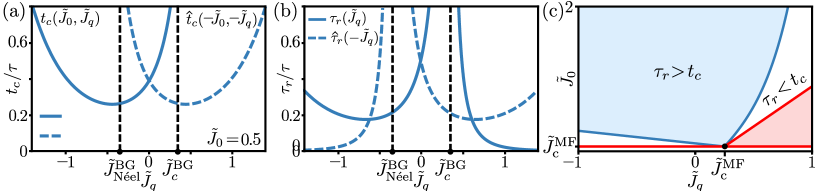
Figure S5: Parity symmetry for the staggered magnetization and the MF dynamical phase diagram. In all panels we consider a lattice with $\bar{z}=4$. (a)-(b) Critical time (a) and relaxation time (b) as a function of the quench temperature $\tilde{J}_{q}$. The dashed lines correspond to the staggered magnetization dynamics, for which a parity symmetry applies w.r.t. the temperature $\tilde{J}\rightarrow-\tilde{J}$ (see Eq. (S69)). (c) Dynamical phase diagram for the MF critical time $t^{\rm MF}_{c}$ and relaxation $\tau^{\rm MF}_{r}$ time. The red area is forbidden since $\tilde{J}_{0}>\tilde{J}_{q}$. Inside the blue area, the relaxation time is larger than the critical time. The dark blue phase boundary where $t^{\rm MF}_{c}=\tau^{\rm MF}_{r}$ is given by Eq. (S72). The MF critical point reads $\tilde{J}^{\rm MF}_{c}\equiv 1/\bar{z}$. Fig. 2f in the Letter shows the BG dynamical phase diagram.

S8 Parity symmetry for the staggered magnetization

Let us define the staggered magnetization $\hat{m}\in[-1,1]$ in the Ising model as

$$\hat{m}\equiv N^{-1}\sum_{i=1}^{N}(-\sigma_{i})^{i}.$$ (S68)

For perfectly anti-ferromagnetic order we have $\hat{m}=\pm 1$, and for anti-ferromagnetic disorder $\hat{m}=0$. Based on the works in Katsura and Takizawa (1974); Ono (1984); Peruggi et al. (1983) we know that the BG free energy density $\tilde{\rm f}_{\rm BG}(m;\tilde{J})$ obeys the following parity symmetry w.r.t. the staggered magnetization

$$\tilde{\rm f}_{\rm BG}(m;\tilde{J})=\tilde{\rm f}_{\rm BG}(\hat{m};-\tilde{J}).$$ (S69)

Therefore, our results for the critical time, relaxation time, and dynamical phase diagram also apply for dynamics of staggered magnetization upon inverting the temperature $\tilde{J}\rightarrow-\tilde{J}$. In Fig. S5a-b we depict the critical time $\hat{t}_{c}$ (a) and relaxation time $\hat{\tau}_{r}$ (b) for the dynamics of the staggered magnetization with the blue dashed lines.

S9 MF dynamical phase diagram

Fig. S5c depicts the MF dynamical phase diagram. To obtain the blue shaded area where $\tau^{\rm MF}_{r}>t^{\rm MF}_{c}$, we first compute the MF critical time. Inserting the MF transition rates and free energy density into Eq. (7) in the Letter we obtain the MF critical time

$$t^{\rm MF}_{c}(\tilde{J}_{0},\tilde{J}_{q})=\frac{1}{4(1-\bar{z}J_{q})}\ln{\left(\frac{\bar{z}\tilde{J}_{q}-\bar{z}\tilde{J}_{0}}{1-\bar{z}\tilde{J}_{0}}\right)},$$ (S70)

which is also reported in Meibohm and Esposito (2022a); Külske and Le Ny (2007); Ermolaev and Külske (2010) for $\bar{z}=1$. The MF relaxation time is given by $\tau^{\rm MF}_{r}(\tilde{J}_{q}){\equiv}1/4w^{\pm}_{\rm MF}(\bar{m};\tilde{J}_{q})\tilde{\rm f}^{\prime\prime}_{\rm MF}(\bar{m};\tilde{J}_{q})$, where $\bar{m}=\arg\min_{m}\tilde{\rm f}_{\rm MF}(m;\tilde{J}_{q})$ is given by the transcendental equation

$$\bar{m}=\tanh{(\bar{z}\tilde{J}_{q}\bar{m})}.$$ (S71)

Equating $t^{\rm MF}_{c}$ and $\tau^{\rm MF}_{r}$ we obtain the dark blue boundary line

$$\bar{z}\tilde{J}^{\dagger}_{0}=\frac{\bar{z}\tilde{J}_{q}\exp{\left(\frac{2(1+\bar{m})(\bar{z}\tilde{J}_{q}-1)}{1-(1-\bar{m}^{2})\bar{z}\tilde{J}_{q}}\mathrm{e}^{-\bar{z}\bar{m}\tilde{J}_{q}}\right)}-1}{\exp{\left(\frac{2(1+\bar{m})(\bar{z}\tilde{J}_{q}-1)}{1-(1-\bar{m}^{2})\bar{z}\tilde{J}_{q}}\mathrm{e}^{-\bar{z}\bar{m}\tilde{J}_{q}}\right)}-1}.$$ (S72)

For $\tilde{J}_{0}>\tilde{J}^{\dagger}_{0}$ (blue region) the MF relaxation time is larger than the critical time, i.e. $\tau^{\rm MF}_{r}>t^{\rm MF}_{c}$. For $1/\bar{z}<\tilde{J}_{0}<\tilde{J}^{\dagger}_{0}$ (white region) the MF critical time is larger than the relaxation time.