Causal Proxy Models for Concept-based Model Explanations

Abstract

Explainability methods for NLP systems encounter a version of the fundamental problem of causal inference: for a given ground-truth input text, we never truly observe the counterfactual texts necessary for isolating the causal effects of model representations on outputs. In response, many explainability methods make no use of counterfactual texts, assuming they will be unavailable. In this paper, we show that robust causal explainability methods can be created using approximate counterfactuals, which can be written by humans to approximate a specific counterfactual or simply sampled using metadata-guided heuristics. The core of our proposal is the Causal Proxy Model (CPM). A CPM explains a black-box model $\mathcal{N}{}$ because it is trained to have the same actual input/output behavior as $\mathcal{N}{}$ while creating neural representations that can be intervened upon to simulate the counterfactual input/output behavior of $\mathcal{N}{}$. Furthermore, we show that the best CPM for $\mathcal{N}{}$ performs comparably to $\mathcal{N}{}$ in making factual predictions, which means that the CPM can simply replace $\mathcal{N}{}$, leading to more explainable deployed models. Our code is available at https://github.com/frankaging/Causal-Proxy-Model.

1 Introduction

The gold standard for explanation methods in AI should be to elucidate the causal role that a model’s representations play in its overall behavior – to truly explain why the model makes the predictions it does. Causal explanation methods seek to do this by resolving the counterfactual question of what the model would do if input $X$ were changed to a relevant counterfactual version $X^{\prime}$. Unfortunately, even though neural networks are fully observed, deterministic systems, we still encounter the fundamental problem of causal inference (Holland, 1986): for a given ground-truth input $X$, we never observe the counterfactual inputs $X^{\prime}$ necessary for isolating the causal effects of model representations on outputs. The issue is especially pressing in domains where it is hard to synthesize approximate counterfactuals. In response to this, explanation methods typically do not explicitly train on counterfactuals at all.

In this paper, we show that robust explanation methods for NLP models can be obtained using texts approximating true counterfactuals. The heart of our proposal is the Causal Proxy Model (CPM). CPMs are trained to mimic both the factual and counterfactual behavior of a black-box model $\mathcal{N}{}$. We explore two different methods for training such explainers. These methods share a distillation-style objective that pushes them to mimic the factual behavior of $\mathcal{N}{}$, but they differ in their counterfactual objectives. The input-based method $\text{CPM{}}_{\text{IN}}$ appends to the factual input a new token associated with the counterfactual concept value. The hidden-state method $\text{CPM{}}_{\text{HI}}$ employs the Interchange Intervention Training (IIT) method of Geiger et al. (2022) to localize information about the target concept in specific hidden states. Figure 1 provides a high-level overview.

We evaluate these methods on the CEBaB benchmark for causal explanation methods (Abraham et al., 2022), which provides large numbers of original examples (restaurant reviews) with human-created counterfactuals for specific concepts (e.g., service quality), with all the texts labeled for their concept-level and text-level sentiment. We consider two types of approximate counterfactuals derived from CEBaB: texts written by humans to approximate a specific counterfactual, and texts sampled using metadata-guided heuristics. Both approximate counterfactual strategies lead to state-of-the-art performance on CEBaB for both $\text{CPM{}}_{\text{IN}}$ and $\text{CPM{}}_{\text{HI}}$.

We additionally identify two other benefits of using CPMs to explain models. First, both $\text{CPM{}}_{\text{IN}}$ and $\text{CPM{}}_{\text{HI}}$ have factual performance comparable to that of the original black-box model $\mathcal{N}{}$ and can explain their own behavior extremely well. Thus, the CPM for $\mathcal{N}{}$ can actually replace $\mathcal{N}{}$, leading to more explainable deployed models. Second, $\text{CPM{}}_{\text{HI}}$ models localize concept-level information in their hidden representations, which makes their behavior on specific inputs very easy to explain. We illustrate this using Path Integrated Gradients (Sundararajan et al., 2017), which we adapt to allow input-level attributions to be mediated by the intermediate states that were targeted for localization. Thus, while both $\text{CPM{}}_{\text{IN}}$ and $\text{CPM{}}_{\text{HI}}$ are comparable as explanation methods according to CEBaB, the qualitative insights afforded by $\text{CPM{}}_{\text{HI}}$ models may given them the edge when it comes to explanations.

2 Related Work

Understanding model behavior serves many goals for large-scale AI systems, including transparency (Kim, 2015; Lipton, 2018; Pearl, 2019; Ehsan et al., 2021), trustworthiness (Ribeiro et al., 2016; Guidotti et al., 2018; Jacovi & Goldberg, 2020; Jakesch et al., 2019), safety (Amodei et al., 2016; Otte, 2013), and fairness (Hardt et al., 2016; Kleinberg et al., 2017; Goodman & Flaxman, 2017; Mehrabi et al., 2021). With CPMs, our goal is to achieve explanations that are causally motivated and concept-based, and so we concentrate here on relating existing methods to these two goals.

Feature attribution methods estimate the importance of features, generally by inspecting learned weights directly or by perturbing features and studying the effects this has on model behavior (Molnar, 2020; Ribeiro et al., 2016). Gradient-based feature attribution methods extend this general mode of explanation to the hidden representations in deep networks (Zeiler & Fergus, 2014; Springenberg et al., 2014; Binder et al., 2016; Shrikumar et al., 2017; Sundararajan et al., 2017). Concept Activation Vectors (CAVs; Kim et al. 2018; Yeh et al. 2020) can also be considered feature attribution methods, as they probe for semantically meaningful directions in the model’s internal representations and use these to estimate the importance of concepts on the model predictions. While some methods in this space do have causal interpretations (e.g., Sundararajan et al. 2017; Yeh et al. 2020), most do not. In addition, most of these methods offer explanations in terms of specific (sets of) features/neurons. (Methods based on CAVs operate directly in terms of more abstract concepts.)

Intervention-based methods study model representations by modifying them in systematic ways and observing the resulting model behavior. These methods are generally causally motivated and allow for concept-based explanations. Examples of methods in this space include causal mediation analysis (Vig et al., 2020; De Cao et al., 2021; Ban et al., 2022), causal effect estimation (Feder et al., 2020; Elazar et al., 2021; Abraham et al., 2022; Lovering & Pavlick, 2022), tensor product decomposition (Soulos et al., 2020), and causal abstraction analysis (Geiger et al., 2020; 2021). CPMs are most closely related to the method of IIT (Geiger et al., 2021), which extends causal abstraction analysis to optimization.

Probing is another important class of explanation method. Traditional probes do not intervene on the target model, but rather only seek to find information in it via supervised models (Conneau et al., 2018; Tenney et al., 2019) or unsupervised models (Clark et al., 2019; Manning et al., 2020; Saphra & Lopez, 2019). Probes can identify concept-based information, but they cannot offer guarantees that probed information is relevant for model behavior (Geiger et al., 2021). For causal guarantees, it is likely that some kind of intervention is required. For example, Elazar et al. (2021) and Feder et al. (2020) remove information from model representations to estimate the causal role of that information. Our CPMs employ a similar set of guiding ideas but are not limited to removing information.

Counterfactual explanation methods aim to explain model behavior by providing a counterfactual example that changes the model behavior (Goyal et al., 2019; Verma et al., 2020; Wu et al., 2021). Counterfactual explanation methods are inherently causal. If they can provide counterfactual examples with regard to specific concepts, they are also concept-based.

Some explanation methods train a model making explicit use of intermediate variables representing concepts. Manipulating these intermediate variables at inference time yields causal concept-based model explanations (Koh et al., 2020; Künzel et al., 2019).

Evaluating methods in this space has been a persistent challenge. In prior literature, explanation methods have often been evaluated against synthetic datasets (Feder et al., 2020; Yeh et al., 2020). In response, Abraham et al. (2022) introduced the CEBaB dataset, which provides a human-validated concept-based dataset to truthfully evaluate different causal concept-based model explanation methods. Our primary evaluations are conducted on CEBaB.

3 Causal Proxy Model (CPM)

(a) A structural causal model leading to an actual text $x_{u,v}$ and its counterfactual text $x_{u,v}^{{C_{i}}\leftarrow{c^{\prime}}}$. $U$ is an exogenous variable over experiences, $c_{1},\ldots,c_{k}$ are mediating concepts, and $V$ is an exogenous variable capturing the writing experience. At right, we create a counterfactual in which concept $C_{i}$ takes on a different value. Unfortunately, we cannot truly create such counterfactual situations and so we never observe pairs of texts like these. Thus, we must rely on approximate counterfactuals.

Let $x_{u,v}$ be a text written in situation $({u},{v})$: Human-created $\tilde{x}_{u,v}^{{C_{i}}\leftarrow{c^{\prime}}}$ Crowdworker edit of $x_{u,v}$ to express that $C_{i}$ had value $c^{\prime}$, seeking to keep all else constant. Metadata-sampled $\tilde{x}_{u,v}^{{C_{i}}\leftarrow{c^{\prime}}}$ Sampled text expressing that $C_{i}$ has value $c^{\prime}$ but agreeing with $x_{u,v}$ on all other concepts.

(b) Approximate counterfactuals. In the human-created strategy, humans revise an attested text to try to express a particular counterfactual, seeking to simulate a causal intervention. In the metadata-sampled strategy, we find a separate text that aligns with the original for the value $u$ insofar as it expresses all the same concepts except for the target concept $C_{i}$.

(c) $\mathcal{L}_{\text{Mimic}}$: All CPMs (bottom) are trained to mimic the behavior of the neural model $\mathcal{N}{}$ to be explained (top) for all factual inputs $x_{u,v}$.

(d) $\mathcal{L}_{\text{IN}}$: Examples $x_{u,v}$ and $\tilde{x}_{u,v}^{{C_{i}}\leftarrow{c^{\prime}}}$ are an approximate counterfactual pair. The CPM is given $x_{u,v}$ augmented with a special token $t_{{C_{i}}\leftarrow{c^{\prime}}}$ and trained to mimic the target model $\mathcal{N}{}$ when its input is $\tilde{x}_{u,v}^{{C_{i}}\leftarrow{c^{\prime}}}$.

(e) $\mathcal{L}_{\text{HI}}$: Examples $x_{u,v}$ and $\tilde{x}_{u,v}^{{C_{i}}\leftarrow{c^{\prime}}}$ are an approximate counterfactual pair. The CPM (middle) is given input $x_{u,v}$. The objective is for it to mimic $\mathcal{N}{}$ (top) given $\tilde{x}_{u,v}^{{C_{i}}\leftarrow{c^{\prime}}}$, but under the intervention in which specific internal states are changed to those that the CPM computes for input $x_{u^{\prime},v^{\prime}}^{{C_{i}}={c^{\prime}}}$ (bottom), which is a distinct example that is sampled with the only criteria being that it express ${C_{i}}={c^{\prime}}$. The effect of this intervention is to localize information about concept $C_{i}$ at the intervention site, since the only indication the CPM gets about ${C_{i}}\leftarrow{c^{\prime}}$ is via the intervention.

Figure 1: Causal Proxy Model (CPM) summary. Every CPM for model $\mathcal{N}{}$ is trained to mimic the factual behavior of $\mathcal{N}{}$ ($\mathcal{L}_{\text{Mimic}}$). For $\text{CPM{}}_{\text{IN}}$, the counterfactual objective is $\mathcal{L}_{\text{IN}}$. For $\text{CPM{}}_{\text{HI}}$, the counterfactual objective is $\mathcal{L}_{\text{HI}}$.

Causal Proxy Models (CPMs) are causal concept-based explanation methods. Given a factual input $x_{u,v}$ and a description of a concept intervention ${C_{i}}\leftarrow{c^{\prime}}$, they estimate the effect of the intervention on model output. The present section introduces our two core CPM variants in detail. We concentrate here on introducing the structure of these models and their objectives, and we save discussion of associated metrics for explanation methods for Section 4.

A Structural Causal Model

Our discussion is grounded in the causal model depicted in Figure 1(a), which aligns well with the CEBaB benchmark. Two exogenous variables $U$ and $V$ together represent the complete state of the world and generate some textual data $X$. The effect of exogenous variable $U$ on the data $X$ is completely mediated by a set of intermediate variables $C_{1},C_{2}\dots,C_{k}$, which we refer to as concepts. Therefore, we can think of $U$ as the part of the world that gives rise to these concepts $\{C\}_{1}^{k}$.

Using this causal model, we can describe counterfactual data – data that arose under a counterfactual state of the world (right diagram in Figure 1(a)). Our factual text is $x_{u,v}$, and we use $x_{u,v}^{{C_{i}}\leftarrow{c^{\prime}}}$ for the counterfactual text obtained by intervening on concept $C_{i}$ to set its value to $c^{\prime}$. The counterfactual $x_{u,v}^{{C_{i}}\leftarrow{c^{\prime}}}$ describes the output when the value of $C_{i}$ is set to $c^{\prime}$, all else being held equal.

Approximate Counterfactuals

Unfortunately, pairs like $({x_{u,v}},{x_{u,v}^{{C_{i}}\leftarrow{c^{\prime}}}})$ are never observed, and thus we need strategies for creating approximate counterfactuals $\tilde{x}_{u,v}^{{C_{i}}\leftarrow{c^{\prime}}}$. Figure 1(b) describes the two strategies we use in this paper. In the human-created strategy, we rely on a crowdworker to edit $x_{u,v}$ to achieve a particular counterfactual goal – say, making the evaluation of the restaurant’s food negative. CEBaB contains an abundance of such pairs $({x_{u,v}},{\tilde{x}_{u,v}^{{C_{i}}\leftarrow{c^{\prime}}}})$. However, CEBaB is unusual in having so many human-created approximate counterfactuals, so we also explore a simpler strategy in which $\tilde{x}_{u,v}^{{C_{i}}\leftarrow{c^{\prime}}}$ is sampled with the requirement that it match $x_{u,v}$ on all concepts but sets $C_{i}$ to $c^{\prime}$. This strategy is supported in many real-world datasets – for example, the OpenTable reviews underlying CEBaB all have the needed metadata (Abraham et al., 2022).

$\text{CPM{}}_{\text{IN}}$: Input-based CPM

To train $\text{CPM{}}_{\text{IN}}$, we associate a new randomly initialized token $t_{{C_{i}}\leftarrow{c^{\prime}}}$ with each unique intervention description ${C_{i}}\leftarrow{c^{\prime}}$. Given a dataset of approximate counterfactual pairs $({x_{u,v}},{\tilde{x}_{u,v}^{{C_{i}}\leftarrow{c^{\prime}}}})$ and a black-box model $\mathcal{N}{}$, we train a new $\text{CPM{}}_{\text{IN}}$ model $\mathcal{P}$ under a weighted sum of the following objectives:

$$\mathcal{L}_{\text{Mimic}} =\text{CE}_{\text{S}}\big{(}\mathcal{N}{}(x_{u,v}),\mathcal{P}(x_{u,v})\big{)}$$ (1)

$$\mathcal{L}_{\text{IN}} =\text{CE}_{\text{S}}\big{(}\mathcal{N}{}(\tilde{x}_{u,v}^{{C_{i}}\leftarrow{c^{\prime}}}),\mathcal{P}(x_{u,v};t_{{C_{i}}\leftarrow{c^{\prime}}})\big{)}$$ (2)

where $x_{u,v};t_{{C_{i}}\leftarrow{c^{\prime}}}$ in Eqn. 2 denotes the concatenation of the factual input and the token describing the intervention. $\text{CE}_{\text{S}}$ represents the smoothed cross-entropy loss (Hinton et al., 2015), measuring the divergence between the output logits of both models. The objective in Eqn. 1 pushes $\mathcal{P}$ to predict the same output as $\mathcal{N}{}$ under conventional circumstances (Figure 1(c)), while Eqn. 2 pushes $\mathcal{P}$ to predict the counterfactual behavior of $\mathcal{N}{}$ when a descriptor of the intervention is given (Figure 1(d)).

At inference time, approximate counterfactuals are inaccessible. To explain model $\mathcal{N}{}$, we append the newly learned descriptor tokens $t_{{C_{i}}\leftarrow{c^{\prime}}}$ to a factual input, upon which $\mathcal{P}$ predicts a counterfactual output for this input, used to estimate the counterfactual behavior of $\mathcal{N}{}$ under this intervention.

$\text{CPM{}}_{\text{HI}}$: Hidden-state CPM

Our $\text{CPM{}}_{\text{HI}}$ models are trained on the same data and with the same set of goals as $\text{CPM{}}_{\text{IN}}$, to mimic both the factual and counterfactual behavior of $\mathcal{N}{}$. The key difference is how the information about the intervention ${C_{i}}\leftarrow{c^{\prime}}$ is exposed to the model. Specifically, we adapt Interchange Intervention Training  (Geiger et al., 2022) to train our $\text{CPM{}}_{\text{HI}}$ models for concept-based model explanation.

A conventional intervention on a hidden representation $H$ of a neural network $\mathcal{N}{}$ fixes the value of the representation $H$ to a constant. In an interchange intervention, we instead fix $H$ to the value it would have been when processing a separate source input $s$. The result of the interchange intervention is a new model. Formally, we describe this new model as $\mathcal{N}_{H\leftarrow H_{s}}$, where $\leftarrow$ is the conventional intervention operator and $H_{s}$ is the value of hidden representation $H$ when processing input $s$.

Given a dataset of approximate counterfactual input pairs $({x_{u,v}},{\tilde{x}_{u,v}^{{C_{i}}\leftarrow{c^{\prime}}}})$ and a black-box model $\mathcal{N}{}$, we train a new $\text{CPM{}}_{\text{HI}}$ model $\mathcal{P}$ under a weighted sum of the previous factual objective (Eqn. 1) and the following counterfactual objective:

$$\mathcal{L}_{\text{HI}} =\text{CE}_{\text{S}}\big{(}\mathcal{N}{}(\tilde{x}_{u,v}^{{C_{i}}\leftarrow{c^{\prime}}}),\mathcal{P}_{H^{C_{i}}\leftarrow H_{s}^{C_{i}}}(x_{u,v})\big{)}$$ (3)

Here $H^{C_{i}}$ are hidden states designated for concept $C_{i}$. In essence, we train $\mathcal{P}$ to fully mediate the effect of intervening on $C_{i}$ in the hidden representation $H^{C_{i}}$. The source input $s$ is any input $x_{u^{\prime},v^{\prime}}^{{C_{i}}={c^{\prime}}}$ that has ${C_{i}}={c^{\prime}}$. As $\mathcal{P}$ only receives information about the concept-level intervention ${C_{i}}\leftarrow{c^{\prime}}$ via the interchange intervention $H^{C_{i}}\leftarrow H_{s}^{C_{i}}$, the model is forced to store all causally relevant information with regard to $C_{i}$ in the corresponding hidden representation. This process is described in Figure 1(e).

In the ideal situation, the source input $x_{u^{\prime},v^{\prime}}^{{C_{i}}={c^{\prime}}}$ and $x_{u,v}$ share the same value only for $C_{i}$ and differ on all others, so that the counterfactual signal needed for localization is pure. However, we do not insist on this when we sample. In addition, we allow null effect pairs in which $x_{u,v}$ and $\tilde{x}_{u,v}^{{C_{i}}\leftarrow{c^{\prime}}}$ are identical. For additional details on this sampling procedure, see Appendix A.2.

At inference time, approximate counterfactuals are inaccessible, as before. To explain model $\mathcal{N}{}$ with regard to intervention ${C_{i}}\leftarrow{c^{\prime}}$, we manipulate the internal states of model $\mathcal{P}$ by intervening on the localized representation $H^{C_{i}}$ for concept $C_{i}$. To achieve this, we sample a source input $x_{u^{\prime},v^{\prime}}^{{C_{i}}={c^{\prime}}}$ from the train set as any input $x$ that has ${C_{i}}={c^{\prime}}$ to derive $H_{s}^{C_{i}}$.

4 Experiment Setup

4.1 Causal Estimation-Based Benchmark (CEBaB)

CEBaB (Abraham et al., 2022) is a large benchmark of high-quality, labeled approximate counterfactuals for the task of sentiment analysis on restaurant reviews. The benchmark was created starting from a set of 2,299 original restaurant reviews from OpenTable. For each of these original reviews, approximate counterfactual examples were written by human annotators; the annotators were tasked to edit the original text to reflect a specific intervention, like ‘change the food evaluation from negative to positive’ or ‘change the service evaluation from positive to unknown’. In this way, the original reviews were expanded with approximate counterfactuals to a total of 15,089 texts. The groups of originals and corresponding approximate counterfactuals are partitioned over train, dev, and test sets. The pairs in the development and test set are used to benchmark explanation methods.

Each text in CEBaB was labeled by five crowdworkers with a 5-star sentiment score. In addition, each text was annotated at the concept level for four mediating concepts $\{C_{\text{ambiance}}$, $C_{\text{food}}$, $C_{\text{noise}}$, and $C_{\text{service}}\}$, using the labels $\{\text{negative},\text{unknown},\text{positive}\}$, again with five crowdworkers annotating each concept-level label. We refer to Appendix A.1 and Abraham et al. 2022 for additional details.

As discussed above (Section 3 and Figure 1(b)), we consider two sources of approximate counterfactuals using CEBaB. For human-created counterfactuals, we use the edited restaurant reviews of the train set. For metadata-sampled counterfactuals, we sample factual inputs from the train set that have the desired combination of mediating concepts. Using all the human-created edits leads to 19,684 training pairs of factuals and corresponding approximate counterfactuals. Sampling counterfactuals leads to 74,574 pairs. We use these approximate counterfactuals to train explanation methods. Appendix A.2 provides more information about our pairing process.

4.2 Evaluation Metrics

Much of the value of a benchmark like CEBaB derives from its support for directly calculating the Estimated Individual Causal Concept Effect ($\widehat{\text{ICaCE}}_{\mathcal{N}{}}$) for a model $\mathcal{N}{}$ given a human-generated approximate counterfactual pair $({x_{u,v}},{\tilde{x}_{u,v}^{{C_{i}}\leftarrow{c^{\prime}}}})$:

$$\widehat{\text{ICaCE}}_{\mathcal{N}}({x_{u,v}},{\tilde{x}_{u,v}^{{C_{i}}\leftarrow{c^{\prime}}}})=\mathcal{N}{}(\tilde{x}_{u,v}^{{C_{i}}\leftarrow{c^{\prime}}})-\mathcal{N}{}(x_{u,v})$$ (4)

This is simply the difference between the vectors of output scores for the two examples.

We do not expect to have pairs $({x_{u,v}},{\tilde{x}_{u,v}^{{C_{i}}\leftarrow{c^{\prime}}}})$ at inference time, and this is what drives the development of explanation methods $\mathcal{E}_{\mathcal{N}{}}$ that estimate this quantity using only a factual input $x_{u,v}$ and a description of the intervention ${C_{i}}\leftarrow{c^{\prime}}$. To benchmark such methods, we follow Abraham et al. (2022) in using the ICaCE-Error:

$$\text{ICaCE-Error}_{\mathcal{N}}^{\mathcal{D}}(\mathcal{E})=\frac{1}{\left|\mathcal{D}\right|}\negthickspace\sum_{({x_{u,v}},{\tilde{x}_{u,v}^{{C_{i}}\leftarrow{c^{\prime}}}})\in\mathcal{D}}\negthickspace\!\!\!\!\mathsf{Dist}\big{(}\widehat{\text{ICaCE}}_{\mathcal{N}}(({x_{u,v}},{\tilde{x}_{u,v}^{{C_{i}}\leftarrow{c^{\prime}}}})),\mathcal{E}_{\mathcal{N}}(x_{u,v};{C_{i}}\leftarrow{c^{\prime}})\big{)}$$ (5)

Here, we assume that $\mathcal{D}$ is a dataset consisting entirely of approximate counterfactual pairs $({x_{u,v}},{\tilde{x}_{u,v}^{{C_{i}}\leftarrow{c^{\prime}}}})$. $\mathsf{Dist}$ measures the distance between the $\widehat{\text{ICaCE}}_{\mathcal{N}{}}$ for the model $\mathcal{N}{}$ and the effect predicted by the explanation method. Abraham et al. (2022) consider three values for $\mathsf{Dist}$: L2, which captures both direction and magnitude; Cosine distance, which captures the direction of effects but not their magnitude; and NormDiff (absolute difference of L2 norms), which captures magnitude but not direction. We report all three metrics.

4.3 Baseline Methods

$\text{BEST}_{\text{CEBaB}}$

We compare our results with the best results obtained on the CEBaB benchmark. Crucially, $\text{BEST}_{\text{CEBaB}}$ is not a single method, but rather pools together the best result obtained by any explanation method previously benchmarked on the CEBaB dataset, for every combination of model and metric.

S-Learner

Our version of S-Learner (Künzel et al., 2019) learns to mimic the factual behavior of black-box model $\mathcal{N}{}$ while making the intermediate concepts explicit. Given a factual input, a finetuned BERT model $\mathcal{B}$ first predicts values for the intermediate concepts. Then, a logistic regression model $\mathsf{LR}_{\mathcal{N}{}}$ is trained to map these intermediate concept values to the factual output of black-box model $\mathcal{N}{}$, under the following objective.

$$\mathcal{L}_{\text{Mimic}}^{\text{S},\mathcal{B}}=\text{CE}_{\text{S}}\big{(}\mathcal{N}{}(x_{u,v}),\mathsf{LR}_{\mathcal{N}{}}(\mathcal{B}(x_{u,v}))\big{)}$$ (6)

By intervening on the intermediate predicted concept values at inference-time, we can hope to simulate the counterfactual behavior of $\mathcal{N}{}$:

$$\mathcal{E}_{\mathcal{N}}^{\text{S},\mathcal{B}}(x_{u,v};{C_{i}}\leftarrow{c^{\prime}})=\mathsf{LR}_{\mathcal{N}{}}((\mathcal{B}(x_{u,v}))_{{C_{i}}\leftarrow{c^{\prime}}})-\mathsf{LR}_{\mathcal{N}{}}(\mathcal{B}(x_{u,v}))$$ (7)

When using S-Learner in conjunction with approximate counterfactual inputs at train-time, we simply add this counterfactual data on top of the observational data that is typically used to train S-Learner.

GPT-3

Large language models such as GPT-3 (175B) have shown extraordinary power in terms of in-context learning (Brown et al., 2020). We use GPT-3 to generate a new approximate counterfactual at inference time given a factual input and a descriptor of the intervention. This generated counterfactual is directly used to estimate the change in model behavior:

$$\mathcal{E}_{\mathcal{N}}^{\text{GPT-3}}(x_{u,v};{C_{i}}\leftarrow{c^{\prime}})=\mathcal{N}{}(\texttt{GPT-3}(x_{u,v};{C_{i}}\leftarrow{c^{\prime}}))-\mathcal{N}{}(x_{u,v})$$ (8)

We use our train-time approximate counterfactual inputs to construct a prompt for GPT-3. Given this prompt, GPT-3 outputs new approximate counterfactuals given a factual and intervention descriptor. Full details on how these prompts are constructed can be found in Appendix A.7.

4.4 Causal Proxy Models

We train CPMs for the publicly available models released for CEBaB, fine-tuned as five-way sentiment classifiers on the factual data. This includes four model architectures: bert-base-uncased (BERT; Devlin et al. 2019), RoBERTa-base (RoBERTa; Liu et al. 2019), GPT-2 (GPT-2; Radford et al. 2019), and LSTM+GloVe (LSTM; Hochreiter & Schmidhuber 1997; Pennington et al. 2014). All Transformer-based models (Vaswani et al., 2017) have 12 Transformer layers. Before training, each CPM model is initialized with the architecture and weights of the black-box model we aim to explain. Thus, the CPMs are rooted in the factual behavior of $\mathcal{N}{}$ from the start. We include details about our setup in Appendix A.3.

The inference time comparisons for these models are as follows, where $\mathcal{P}$ in Eqn. 9 and Eqn. 10 refers to the CPM model trained under $\text{CPM{}}_{\text{IN}}$ and $\text{CPM{}}_{\text{HI}}$ objectives, respectively:

$$\mathcal{E}_{\mathcal{N}}^{\text{CPM{}}_{\text{IN}}}(x_{u,v};{C_{i}}\leftarrow{c^{\prime}}) =\mathcal{P}(x_{u,v};t_{{C_{i}}\leftarrow{c^{\prime}}})-\mathcal{N}(x_{u,v})$$ (9)

$$\mathcal{E}_{\mathcal{N}}^{\text{CPM{}}_{\text{HI}}}(x_{u,v};{C_{i}}\leftarrow{c^{\prime}}) =\mathcal{P}_{H^{C_{i}}\leftarrow H_{s}^{C_{i}}}(x_{u,v})-\mathcal{N}(x_{u,v})$$ (10)

Here, $s$ is a source input with ${C_{i}}={c^{\prime}}$, and $H^{C_{i}}$ is the neural representation associated with $C_{i}$ which takes value $H_{s}^{C_{i}}$ on the source input $s$. As $H^{C_{i}}$, for BERT we use slices of width 192 taken from the 1st intermediate token of the 10th layer. For RoBERTa, we use the 8th layer instead. For GPT-2, we pick the final token of the 12th layer, again with slice width of 192. For LSTM, we consider slices of the attention-gated sentence embedding with width 64. Appendix A.5 studies the impact of intervention location and size.

Following the guidance on IIT given by Geiger et al. (2022), we train $\text{CPM{}}_{\text{HI}}$ with an additional multi-task objective as,

$$\mathcal{L}_{\text{Multi}}=\sum_{C_{i}\in C}\text{CE}(\mathsf{MLP}(H_{x}^{C_{i}}),c)$$ (11)

where our probe is parameterized by a multilayer perceptron $\mathsf{MLP}$, and $H_{x}^{C_{i}}$ is the value of hidden representation for the concept $C_{i}$ when processing input $x$ with a concept label of $c$ for $C_{i}$.

5 Results

			no counterfactuals			sampled counterfactuals					human-created counterfactuals
								(ours)	(ours)				(ours)	(ours)
Model	Metric		BEST${}_{\text{CEBaB}}$	S-Learner		S-Learner	GPT-3	$\text{CPM{}}_{\text{IN}}$	$\text{CPM{}}_{\text{HI}}$		S-Learner	GPT-3	$\text{CPM{}}_{\text{IN}}$	$\text{CPM{}}_{\text{HI}}$
BERT	L2		0.74 ([v]0.02)	0.74 ([v]0.02)		0.74 ([v]0.02)	0.71 ([v]0.01)	0.63 ([v]0.01)	0.60 ([v]0.01)		0.73 ([v]0.02)	0.45 ([v]0.01)	0.45 ([v]0.02)	0.45 ([v]0.03)
	Cosine		0.59 ([v]0.03)	0.63 ([v]0.01)		0.63 ([v]0.01)	0.51 ([v]0.00)	0.46 ([v]0.00)	0.45 ([v]0.00)		0.60 ([v]0.01)	0.36 ([v]0.00)	0.35 ([v]0.00)	0.36 ([v]0.04)
	NormDiff		0.44 ([v]0.01)	0.54 ([v]0.02)		0.53 ([v]0.02)	0.35 ([v]0.01)	0.39 ([v]0.01)	0.38 ([v]0.00)		0.52 ([v]0.02)	0.25 ([v]0.00)	0.24 ([v]0.01)	0.27 ([v]0.01)
RoBERTa	L2		0.78 ([v]0.01)	0.78 ([v]0.01)		0.78 ([v]0.00)	0.74 ([v]0.01)	0.66 ([v]0.01)	0.67 ([v]0.02)		0.77 ([v]0.00)	0.48 ([v]0.01)	0.46 ([v]0.01)	0.47 ([v]0.03)
	Cosine		0.58 ([v]0.01)	0.64 ([v]0.01)		0.65 ([v]0.01)	0.53 ([v]0.01)	0.46 ([v]0.00)	0.47 ([v]0.00)		0.63 ([v]0.01)	0.39 ([v]0.00)	0.38 ([v]0.01)	0.39 ([v]0.03)
	NormDiff		0.45 ([v]0.00)	0.59 ([v]0.01)		0.58 ([v]0.00)	0.36 ([v]0.00)	0.42 ([v]0.01)	0.45 ([v]0.03)		0.56 ([v]0.00)	0.28 ([v]0.01)	0.26 ([v]0.01)	0.29 ([v]0.05)
GPT-2	L2		0.60 ([v]0.02)	0.60 ([v]0.02)		0.61 ([v]0.01)	0.65 ([v]0.01)	0.55 ([v]0.01)	0.51 ([v]0.01)		0.61 ([v]0.01)	0.43 ([v]0.01)	0.41 ([v]0.01)	0.41 ([v]0.04)
	Cosine		0.59 ([v]0.01)	0.59 ([v]0.01)		0.59 ([v]0.01)	0.52 ([v]0.00)	0.47 ([v]0.01)	0.46 ([v]0.00)		0.59 ([v]0.01)	0.40 ([v]0.00)	0.37 ([v]0.01)	0.39 ([v]0.05)
	NormDiff		0.40 ([v]0.01)	0.40 ([v]0.01)		0.41 ([v]0.01)	0.34 ([v]0.00)	0.32 ([v]0.01)	0.30 ([v]0.00)		0.40 ([v]0.01)	0.24 ([v]0.01)	0.23 ([v]0.01)	0.27 ([v]0.05)
LSTM	L2		0.73 ([v]0.01)	0.73 ([v]0.01)		0.73 ([v]0.01)	0.76 ([v]0.00)	0.66 ([v]0.01)	0.64 ([v]0.02)		0.72 ([v]0.00)	0.49 ([v]0.00)	0.52 ([v]0.00)	0.54 ([v]0.01)
	Cosine		0.64 ([v]0.01)	0.64 ([v]0.01)		0.64 ([v]0.01)	0.57 ([v]0.01)	0.50 ([v]0.00)	0.50 ([v]0.01)		0.63 ([v]0.01)	0.44 ([v]0.00)	0.45 ([v]0.01)	0.46 ([v]0.00)
	NormDiff		0.50 ([v]0.01)	0.53 ([v]0.01)		0.53 ([v]0.00)	0.41 ([v]0.00)	0.42 ([v]0.00)	0.41 ([v]0.01)		0.54 ([v]0.00)	0.30 ([v]0.00)	0.34 ([v]0.01)	0.36 ([v]0.00)

Table 1: CEBaB scores measured in three different metrics on the test set for four different model architectures as a five-class sentiment classification task. Lower is better. Results averaged over three distinct seeds, standard deviations in parentheses. The metrics are described in Section 4. Best averaged result is bolded (including ties) per approximate counterfactual creation strategy.

We first benchmark both CPM variants and our baseline methods on CEBaB. We show that the CPMs achieve state-of-the-art performance, for both types of approximate counterfactuals used during training (Section 5.1). Given the good factual performance achieved by CPMs, we subsequently investigate whether CPMs can be deployed both as predictor and explanation method at the same time (Section 5.2) and find that they can. Finally, we show that the localized representations of $\text{CPM{}}_{\text{HI}}$ give rise to concept-aware feature attributions (Section 5.3). Our supplementary materials report on detailed ablation studies and explore the potential of our methods for model debiasing.

5.1 CEBaB Performance

Table 1 presents our main results. The results are grouped per approximate counterfactual type used during training. Both $\text{CPM{}}_{\text{IN}}$ and $\text{CPM{}}_{\text{HI}}$ beat BEST${}_{\text{CEBaB}}$ in every evaluation setting by a large margin, establishing state-of-the-art explanation performance. Interestingly, $\text{CPM{}}_{\text{HI}}$ seems to slightly outperform $\text{CPM{}}_{\text{IN}}$ using sampled approximate counterfactuals, while slightly underperforming $\text{CPM{}}_{\text{IN}}$ on human-created approximate counterfactuals. Appendix A.6 reports on ablation studies that indicate that, for $\text{CPM{}}_{\text{HI}}$, this state-of-the-art performance is primarily driven by the role of IIT in localizing concepts.

S-Learner, one of the best individual explainers from the original CEBaB paper (Abraham et al., 2022), shows only a marginal improvement when naively incorporating sampled and human-created counterfactuals during training over using no counterfactuals. This indicates that the large performance gains achieved by our CPMs over previous explainers are most likely due to the explicit use of a counterfactual training signal, and not primarily due to the addition of extra (counterfactual) data.

GPT-3 occasionally performs on-par with our CPMs, generally only slightly underperforming our best explainer on human-created counterfactuals, while being significantly worse on sampled counterfactuals. While the GPT-3 explainer also explicitly uses approximate counterfactual data, the results indicate that our proposed counterfactual mimic objectives give better results. The better performance of CPMs when considering sampled counterfactuals over GPT-3 shows that our approach is more robust to the quality of the approximate counterfactuals used. While the GPT-3 explainer is easy to set up (no training required), it might not be suitable for some explanation applications regardless of performance, due to the latency and cost involved in querying the GPT-3 API.

Across the board, explainers trained with human-created counterfactuals are better than those trained with sampled counterfactuals. This shows that the performance of explanation methods depends on the quality of the approximate counterfactual training data. While human counterfactuals give excellent performance, they may be expensive to create. Sampled counterfactuals are cheaper if the relevant metadata is available. Thus, under budgetary constraints, sampled counterfactuals may be more efficient.

Finally, $\text{CPM{}}_{\text{IN}}$ is conceptually the simpler of the two CPM variants. However, we discuss in Section 5.3 how the localized representations of $\text{CPM{}}_{\text{HI}}$ lead to additional explainability benefits.

5.2 Self-Explanation with CPM

As outlined in Section 3, CPMs learn to mimic both the factual and counterfactual behavior of the black-box models they are explaining. We show in Table 2 that our CPMs achieve a factual Macro-F1 score comparable to the black-box finetuned models.

We investigate if we can simply replace the black-box model with our CPM and use the CPM both as factual predictor and counterfactual explainer. To answer this questions, we measure the self-explanation performance of CPMs by simply replacing the black-box model $\mathcal{N}{}$ in Eqn. 5 with our factual CPM predictions at inference time.

Table 3 reports these results. We find that both $\text{CPM{}}_{\text{IN}}$ and $\text{CPM{}}_{\text{HI}}$ achieve better self-explanation performance compared to providing explanations for another black-box model. Furthermore, $\text{CPM{}}_{\text{HI}}$ provides better self-explanation than $\text{CPM{}}_{\text{IN}}$, suggesting our interchange intervention procedure leads the model to localize concept-based information in hidden representations. This shows that CPMs may be viable as replacements for their black-box counterpart, since they provide similar task performance while providing faithful counterfactual explanations of both the black-box model and themselves.

				sampled			human-created
		Fine-		counterfactuals			counterfactuals
Model		tuned		$\text{CPM{}}_{\text{IN}}$	$\text{CPM{}}_{\text{HI}}$		$\text{CPM{}}_{\text{IN}}$	$\text{CPM{}}_{\text{HI}}$
BERT		0.70 ([v]0.01)		0.70 ([v]0.00)	0.67 ([v]0.02)		0.70 ([v]0.01)	0.69 ([v]0.01)
RoBERTa		0.70 ([v]0.00)		0.70 ([v]0.00)	0.69 ([v]0.01)		0.71 ([v]0.01)	0.71 ([v]0.00)
GPT-2		0.65 ([v]0.00)		0.65 ([v]0.00)	0.67 ([v]0.01)		0.66 ([v]0.01)	0.68 ([v]0.00)
LSTM		0.60 ([v]0.01)		0.60 ([v]0.01)	0.56 ([v]0.00)		0.54 ([v]0.00)	0.59 ([v]0.01)

Table 2: Task performance measured as Macro-F1 score on the test set. Results averaged over three distinct seeds; standard deviations in parentheses.

			sampled			human-created
			counterfactuals			counterfactuals
Model	Metric		$\text{CPM{}}_{\text{IN}}$	$\text{CPM{}}_{\text{HI}}$		$\text{CPM{}}_{\text{IN}}$	$\text{CPM{}}_{\text{HI}}$
BERT	L2		0.63 ([v]0.01)	0.52 ([v]0.04)		0.42 ([v]0.02)	0.38 ([v]0.03)
	Cosine		0.46 ([v]0.00)	0.45 ([v]0.01)		0.34 ([v]0.02)	0.30 ([v]0.06)
	NormDiff		0.39 ([v]0.01)	0.33 ([v]0.02)		0.23 ([v]0.01)	0.22 ([v]0.05)
RoBERTa	L2		0.66 ([v]0.01)	0.63 ([v]0.04)		0.40 ([v]0.01)	0.37 ([v]0.04)
	Cosine		0.46 ([v]0.00)	0.48 ([v]0.01)		0.33 ([v]0.01)	0.29 ([v]0.04)
	NormDiff		0.42 ([v]0.01)	0.42 ([v]0.05)		0.21 ([v]0.01)	0.23 ([v]0.05)
GPT-2	L2		0.55 ([v]0.01)	0.41 ([v]0.03)		0.38 ([v]0.01)	0.36 ([v]0.04)
	Cosine		0.47 ([v]0.01)	0.39 ([v]0.02)		0.37 ([v]0.01)	0.35 ([v]0.05)
	NormDiff		0.32 ([v]0.01)	0.25 ([v]0.02)		0.22 ([v]0.01)	0.24 ([v]0.05)
LSTM	L2		0.66 ([v]0.01)	0.41 ([v]0.01)		0.46 ([v]0.00)	0.42 ([v]0.01)
	Cosine		0.50 ([v]0.00)	0.42 ([v]0.02)		0.50 ([v]0.02)	0.40 ([v]0.01)
	NormDiff		0.42 ([v]0.00)	0.25 ([v]0.00)		0.31 ([v]0.00)	0.28 ([v]0.02)

Table 3: Self-explanation CEBaB scores measured in three different metrics on the test set for four different model architectures as a five-class sentiment classification task. Lower is better. Results averaged over three distinct seeds, standard deviations in parentheses.

5.3 Concept-Aware Feature Attribution with $\text{CPM{}}_{\text{HI}}$

We have shown that $\text{CPM{}}_{\text{HI}}$ provides trustworthy explanations (Section 5.1). We now investigate whether $\text{CPM{}}_{\text{HI}}$ learns representations that mediate the effects of different concepts. We adapt Integrated Gradients (IG; Sundararajan et al. 2017) to provide concept-aware feature attributions, by only considering gradients flowing through the hidden representation associated with a given concept. We formalize this version of IG in Appendix A.8.

In Table 4, we compare concept-aware feature attibutions for two variants of $\text{CPM{}}_{\text{HI}}$ (IIT and Multi-task) and the original black-box (Finetuned) model. For IIT we remove the multi-task objective $\mathcal{L}_{\text{Multi}}$ during training and for Multi-task we remove the the interchange intervention objective $\mathcal{L}_{\text{HI}}$. This helps isolate the individual effects of both losses on concept localization. All three models predict a neutral final sentiment score for the considered input, but they show vastly different feature attributions. Only IIT reliably highlights words that are semantically related to each concept. For instance, when we restrict the gradients to flow only through the intervention site of the noise concept, “loud” is the word highlighted the most that contributes negatively. When we consider the service concept, words like “friendly” and “waiter” are highlighted the most as contributing positively. These contrasts are missing for representations of the Multi-task and Finetuned models. Only the IIT training paradigm pushes the model to learn causally localized representations. For the service concept, we notice that the IIT model wrongfully attributes “delicious”. This could be useful for debugging purposes and could be used to highlight potential failure modes of the model.

Model	Predicted	Concept	Score	Word Importance
Finetuned	neutral	ambiance	$+0.03$	[CLS]themusicwastooloud,andthedecorationsweretaste##less,buttheyhadfriendlywaiter##sanddeliciouspasta[SEP]
		food	$+0.11$	[CLS]themusicwastooloud,andthedecorationsweretaste##less,buttheyhadfriendlywaiter##sanddeliciouspasta[SEP]
		noise	$+0.04$	[CLS]themusicwastooloud,andthedecorationsweretaste##less,buttheyhadfriendlywaiter##sanddeliciouspasta[SEP]
		service	$+0.26$	[CLS]themusicwastooloud,andthedecorationsweretaste##less,buttheyhadfriendlywaiter##sanddeliciouspasta[SEP]
Multi-task	neutral	ambiance	$+0.25$	[CLS]themusicwastooloud,andthedecorationsweretaste##less,buttheyhadfriendlywaiter##sanddeliciouspasta[SEP]
		food	$+0.23$	[CLS]themusicwastooloud,andthedecorationsweretaste##less,buttheyhadfriendlywaiter##sanddeliciouspasta[SEP]
		noise	$+0.31$	[CLS]themusicwastooloud,andthedecorationsweretaste##less,buttheyhadfriendlywaiter##sanddeliciouspasta[SEP]
		service	$+0.16$	[CLS]themusicwastooloud,andthedecorationsweretaste##less,buttheyhadfriendlywaiter##sanddeliciouspasta[SEP]
IIT	neutral	ambiance	$-0.24$	[CLS]themusicwastooloud,andthedecorationsweretaste##less,buttheyhadfriendlywaiter##sanddeliciouspasta[SEP]
		food	$+1.11$	[CLS]themusicwastooloud,andthedecorationsweretaste##less,buttheyhadfriendlywaiter##sanddeliciouspasta[SEP]
		noise	$-0.98$	[CLS]themusicwastooloud,andthedecorationsweretaste##less,buttheyhadfriendlywaiter##sanddeliciouspasta[SEP]
		service	$+1.16$	[CLS]themusicwastooloud,andthedecorationsweretaste##less,buttheyhadfriendlywaiter##sanddeliciouspasta[SEP]

Table 4: Visualizations of word importance scores using Integrated Gradient (IG) by restricting gradient flow through the corresponding intervention site of the targeted concept. Our target class pools positive and very positive. Individual word importance is the sum of neuron-level importance scores for each input, normalized to [$-1$, $+1$]. $-1$ means the word contributes the most negatively to predicting the target class (red); $+1$ means the word contributes the most positively (green).

6 Conclusion

We explored the use of approximate counterfactual training data to build more robust causal explanation methods. We introduced Causal Proxy Models (CPMs), which learn to mimic both the factual and counterfactual behaviors of a black-box model $\mathcal{N}{}$. Using CEBaB, a benchmark for causal concept-based explanation methods, we demonstrated that both versions of our technique ($\text{CPM{}}_{\text{IN}}$ and $\text{CPM{}}_{\text{HI}}$) significantly outperform previous explanation methods.

Interestingly, we find that our GPT-3 based explanation method performs on-par with our best CPM model in some settings. While test-time use of GPT-3 as explanation method might not be feasible, we believe this result shows that GPT-3 could be deployed to supplement human-annotation efforts for counterfactual data creation.

Our results suggest that CPMs can be more than just explanation methods. They achieve factual performance on par with the model they aim to explain, and they can explain their own behavior. This paves the way to using them as deployed models that both perform tasks and offer explanations. In addition, the causally localized representations of our $\text{CPM{}}_{\text{HI}}$ variant are very intuitive, as revealed by our concept-aware feature attribution technique. We believe that causal localization techniques could play a vital role in further model explanation efforts.

7 Acknowledgement

This research is supported in part by a grant from Meta AI. Karel D’Oosterlinck was supported through a doctoral fellowship from the Special Research Fund (BOF) of Ghent University.

Appendix A Appendix

A.1 CEBaB Dataset Statistics

Table 5 shows dataset statistics of CEBaB. The variants of CEBaB we consider only impact the train split. The top panel shows the number of observational samples and edits introduced in the CEBaB paper. The bottom panel shows our paired versions, where we create approximate counterfactual pairs. We explore two variants of approximate counterfactuals: human-created and sampled counterfactuals (Section 4.1). The human setting considers all pairs made possible by using all data. The sampling setting considers pairs sampled from only the observational data, as discussed in Section A.2.

Dataset		# train	# dev	# test
CEBaB (observational)		1,755	1,673	1,689
CEBaB (all)		11,728	1,673	1,689
CEBaB (paired, human)		19,684	3,898	3,958
CEBaB (paired, sampling)		74,574	3,898	3,958

Table 5: Dataset statistics.

A.2 Types of Approximate Counterfactual Pairs

Our approximate counterfactual training data comes in paired sentences of (original sentence, approximate counterfactual sentence). The approximate counterfactuals differs from their original counterparts in only one concept value. We consider approximate counterfactual pairs to be symmetric: we use both (original sentence, approximate counterfactual sentence) and (approximate counterfactual sentence, original sentence) as training pairs.

Human-created Counterfactuals

CEBaB contains multiple counterfactual sentences for each original review. To achieve this, the dataset creators asked annotators to edit the original sentence to achieve a specified goal (e.g., ‘change the evaluation of the restaurant’s food to negative’). These originals and corresponding edits form our human pairs.

Metadata-sampled Counterfactuals

Human-created counterfactuals are not always available. With CEBaB, we simulate a second type of approximate counterfactuals by using metadata-guided heuristics: for a given original sentence, we sample a counterfactual from the train set by matching concept labels while allowing only one label to be changed.

During training, we also consider null effect pairs in our sampling setup. These pairs resemble cases where our approximate counterfactual sentence is identical to the original sentence. When training our models on these pairs, we expect our models to predict the same counterfactual and factual output.

A.3 Training Regimes

$\text{CPM{}}_{\text{IN}}$

To train $\text{CPM{}}_{\text{IN}}$, we use the same model architecture as $\mathcal{N}$, and initialize it with the model weights using weights from $\mathcal{N}$. The maximum number of training epochs is set to 30 with a learning rate of $5e^{-5}$ and an effective batch size of 128. The learning rate linearly decays to $0$ over the 30 training epochs. We employ an early stopping strategy for $\text{COS}_{\texttt{ICaCE}}$ over the dev set for an interval of 50 steps with early stopping patience set to 20. We set the max sequence length to 128 and the dropout rate to $0.1$. We take a weighted sum of two objectives as the loss term for training $\text{CPM{}}_{\text{HI}}$. Specifically, we use $[w_{\text{Mimic}},w_{\text{IN}}]=[1.0,3.0]$. For the smoothed cross-entropy loss, we use a temperature of $2.0$.

$\text{CPM{}}_{\text{HI}}$

To train $\text{CPM{}}_{\text{HI}}$, we use the same model architecture as $\mathcal{N}$, and initialize it with the model weights using weights from $\mathcal{N}$. The maximum number of training epochs is set to 30 with a learning rate of $8e^{-5}$ and an effective batch size of 256. We use a higher learning rate of $0.001$ for the LSTM model as it enables quicker convergence. The learning rate linearly decays to $0$ over the 30 training epochs. We employ an early stopping strategy for $\text{COS}_{\texttt{ICaCE}}$ over the dev set for an interval of 10 steps with early stopping patience set to 20. We set the max sequence length to 128 and the dropout rate to $0.1$. We take a weighted sum of three objectives as the loss term for training $\text{CPM{}}_{\text{HI}}$. Specifically, we use $[w_{\text{Mimic}},w_{\text{Multi}},w_{\text{HI}}]=[1.0,1.0,3.0]$. In Appendix A.6, we conduct a set of ablation studies to isolate the individual contributions from each objective. For the smoothed cross-entropy loss, we use a temperature of $2.0$.

Our models are all implemented in PyTorch (Paszke et al., 2019) and using the HuggingFace library (Wolf et al., 2019). All of our results are aggregated over three distinct random seeds. To foster reproducibility, we will release our code repository and model artifacts to the public.

Figure 2: CEBaB scores for different intervention site locations and sizes for $\text{CPM{}}_{\text{HI}}$. The scores are measured in three different metrics on the test set for four different model architectures as a five-class sentiment classification task. Results averaged over three distinct seeds. Task performance as Macro-F1 score is reported when applicable. Shaded areas outline $\pm$ SD.

A.4 Additional Baseline Results

Table 6 shows baselines adapted from Abraham et al. (2022), which contains the present state-of-the-art explanation methods for the CEBaB benchmark. We report the best scores across these explanation methods in Table 1. These baselines are trained without using counterfactual data. Thus, we build additional baselines that use counterfactual data as shown in Table 7. S-Learner is selected as the best performing models and included in Table 1 for comparisons. The equations for the additional baselines are as follows:

$$\mathcal{E}_{\mathcal{N}}^{\text{approx}}(x_{u,v};{C_{i}}\leftarrow{c^{\prime}}) =\mathcal{N}(s^{\text{approx}})-\mathcal{N}(x_{u,v})$$ (12)

$$\mathcal{E}_{\mathcal{N}}^{\text{random}}(x_{u,v};{C_{i}}\leftarrow{c^{\prime}}) =\mathcal{N}(s^{\text{random}})-\mathcal{N}(x_{u,v})$$ (13)

$$\mathcal{E}_{\mathcal{N}}^{\text{CaCE}}({C_{i}}\leftarrow{c^{\prime}}) =\frac{1}{\left|\mathcal{D}^{{C_{i}}\leftarrow{c^{\prime}}}\right|}\negthickspace\sum_{({x_{u,v}},{\tilde{x}_{u,v}^{{C_{i}}\leftarrow{c^{\prime}}}})\in\mathcal{D}^{{C_{i}}\leftarrow{c^{\prime}}}}\negthickspace\!\!\!\!\left(\mathcal{N}\left(\tilde{x}_{u,v}^{{C_{i}}\leftarrow{c^{\prime}}}\right)-\mathcal{N}\left(x_{u,v}\right)\right)$$ (14)

$$\mathcal{E}^{\text{ATE}}({C_{i}}\leftarrow{c^{\prime}}) =\frac{1}{\left|\mathcal{D}^{{C_{i}}\leftarrow{c^{\prime}}}\right|}\negthickspace\sum_{({x_{u,v}},{\tilde{x}_{u,v}^{{C_{i}}\leftarrow{c^{\prime}}}})\in\mathcal{D}^{{C_{i}}\leftarrow{c^{\prime}}}}\negthickspace\!\!\!\!\left(f\left(\tilde{x}_{u,v}^{{C_{i}}\leftarrow{c^{\prime}}}\right)-f\left(x_{u,v}\right)\right)$$ (15)

where $s^{\text{random}}$ is a randomly sampled training input, $s^{\text{approx}}$ is a training input sampled to match the concept-level labels of the true counterfactual under intervention ${C_{i}}\leftarrow{c^{\prime}}$, $\mathcal{D}^{{C_{i}}\leftarrow{c^{\prime}}}$ is the set of all approximate counterfactual training pairs that represent a ${C_{i}}\leftarrow{c^{\prime}}$ intervention, and $f$ is a look-up function that returns the ground-truth label associated with an input.

The signatures of $\mathcal{E}^{\text{ATE}}$ and $\mathcal{E}_{\mathcal{N}}^{\text{CaCE}}$ reflect that they are independent of the specific factual input $x_{u,v}$ considered. Furthermore, $\mathcal{E}^{\text{ATE}}$ is independent of $\mathcal{N}{}$ given that this explainer only uses ground-truth training labels to estimate causal effects.

Model	Metric		Approx†	S-Learner‡	INLP§
BERT	L2		0.81 ([v]0.01)	0.74 ([v]0.02)	0.80 ([v]0.02)
	Cosine		0.61 ([v]0.01)	0.63 ([v]0.01)	0.59 ([v]0.03)
	NormDiff		0.44 ([v]0.01)	0.54 ([v]0.02)	0.73 ([v]0.02)
RoBERTa	L2		0.83 ([v]0.01)	0.78 ([v]0.01)	0.84 ([v]0.01)
	Cosine		0.60 ([v]0.01)	0.64 ([v]0.01)	0.58 ([v]0.01)
	NormDiff		0.45 ([v]0.00)	0.59 ([v]0.01)	0.81 ([v]0.01)
GPT-2	L2		0.72 ([v]0.02)	0.60 ([v]0.02)	0.72 ([v]0.01)
	Cosine		0.59 ([v]0.01)	0.59 ([v]0.01)	1.00 ([v]0.00)
	NormDiff		0.41 ([v]0.01)	0.40 ([v]0.01)	0.58 ([v]0.03)
LSTM	L2		0.86 ([v]0.01)	0.73 ([v]0.01)	0.79 ([v]0.01)
	Cosine		0.64 ([v]0.01)	0.64 ([v]0.01)	0.74 ([v]0.02)
	NormDiff		0.50 ([v]0.01)	0.53 ([v]0.01)	0.60 ([v]0.01)

Table 6: CEBaB scores measured in three different metrics on the test set for four different model architectures as a five-class sentiment classification task. Results are adapted from Abraham et al. (2022). Lower is better; standard deviations over 5 distinct seeds in parentheses. Results are aggregated over all aspects and all directional concept label changes. Details about these evaluation metrics can be found in Section 4. Results are based on ^†Abraham et al. (2022), ^‡ Künzel et al. (2019), and ^§Ravfogel et al. (2020).

			sampled counterfactuals					human-created counterfactuals
				ATE-	CaCE-				ATE-	CaCE-
Model	Metric		Approx	Explainer	Explainer	Random		Approx	Explainer	Explainer	Random
BERT	L2		0.81 ([v]0.01)	0.81 ([v]0.02)	0.81 ([v]0.02)	0.84 ([v]0.02)		0.79 ([v]0.02)	0.81 ([v]0.02)	0.80 ([v]0.02)	0.84 ([v]0.01)
	Cosine		0.60 ([v]0.00)	0.72 ([v]0.01)	0.72 ([v]0.01)	0.53 ([v]0.00)		0.56 ([v]0.01)	0.69 ([v]0.01)	0.69 ([v]0.01)	0.53 ([v]0.00)
	NormDiff		0.44 ([v]0.01)	0.62 ([v]0.02)	0.62 ([v]0.02)	0.55 ([v]0.02)		0.43 ([v]0.01)	0.62 ([v]0.02)	0.64 ([v]0.02)	0.54 ([v]0.02)
RoBERTa	L2		0.83 ([v]0.01)	0.85 ([v]0.00)	0.85 ([v]0.00)	0.87 ([v]0.00)		0.81 ([v]0.01)	0.85 ([v]0.00)	0.84 ([v]0.00)	0.87 ([v]0.00)
	Cosine		0.61 ([v]0.01)	0.73 ([v]0.00)	0.73 ([v]0.01)	0.53 ([v]0.00)		0.57 ([v]0.01)	0.70 ([v]0.00)	0.70 ([v]0.00)	0.53 ([v]0.00)
	NormDiff		0.46 ([v]0.01)	0.67 ([v]0.00)	0.67 ([v]0.00)	0.58 ([v]0.00)		0.44 ([v]0.01)	0.67 ([v]0.00)	0.68 ([v]0.00)	0.59 ([v]0.00)
GPT-2	L2		0.72 ([v]0.02)	0.69 ([v]0.01)	0.68 ([v]0.01)	0.76 ([v]0.00)		0.72 ([v]0.01)	0.68 ([v]0.01)	0.68 ([v]0.01)	0.76 ([v]0.00)
	Cosine		0.59 ([v]0.00)	0.67 ([v]0.00)	0.67 ([v]0.00)	0.56 ([v]0.00)		0.57 ([v]0.00)	0.66 ([v]0.00)	0.65 ([v]0.00)	0.56 ([v]0.00)
	NormDiff		0.40 ([v]0.01)	0.48 ([v]0.01)	0.49 ([v]0.01)	0.47 ([v]0.00)		0.40 ([v]0.00)	0.49 ([v]0.01)	0.50 ([v]0.01)	0.47 ([v]0.01)
LSTM	L2		0.87 ([v]0.00)	0.78 ([v]0.00)	0.78 ([v]0.00)	0.85 ([v]0.00)		0.85 ([v]0.01)	0.78 ([v]0.00)	0.76 ([v]0.00)	0.84 ([v]0.00)
	Cosine		0.65 ([v]0.00)	0.71 ([v]0.00)	0.71 ([v]0.00)	0.57 ([v]0.00)		0.61 ([v]0.00)	0.69 ([v]0.00)	0.68 ([v]0.00)	0.56 ([v]0.00)
	NormDiff		0.50 ([v]0.00)	0.59 ([v]0.00)	0.59 ([v]0.00)	0.55 ([v]0.00)		0.49 ([v]0.00)	0.59 ([v]0.00)	0.61 ([v]0.00)	0.55 ([v]0.00)

Table 7: CEBaB scores for additional baselines we considered. CEBaB scores are measured in three different metrics on the test set for four different model architectures as a five-class sentiment classification task. Lower is better. Results averaged over three distinct seeds, standard deviations in parentheses. Details about these evaluation metrics can be found in Section 4.

A.5 Intervention Site Location and Size

Previous work shows that neurons in different layers and groups can encode different high-level concepts (Vig et al., 2020; Koh et al., 2020). $\text{CPM{}}_{\text{HI}}$ pushes concept-related information to localize at the targeted intervention site (the aligned neural representations for each concept). In this section, we investigate how the location and the size of the intervention site impact $\text{CPM{}}_{\text{HI}}$ performance. We use the optimal location and size found in this study for other results presented in this paper.

Location

For Transformer-based models, we vary the location of the intervention site by intervening on the “[CLS]” token embedding layer $l$. Specifically, we set $l=\{2,4,6,8,10,12\}$. We skip this experiment for non-Transformer-based model (i.e., LSTM) since it only contains a single sentence embedding.

As shown in the top panel of Figure 2, intervention location significantly affects $\text{CPM{}}_{\text{HI}}$ performance. Our results show that layer 10 for BERT, layer 8 for RoBERTa, and layer 12 for GPT-2 lead to the best performance. This suggests layers have different efficacy in terms of information localization. Our results also show that intervening with deeper layers tends to provide better performance. However, for both BERT and RoBERTa, intervening on the last layer results in a slightly worse performance compared to earlier layers. This suggests that leaving Transformer blocks after the intervention site helps localized information to be processed by the neural network.

Size

For Transformer-based models, we change the size of the intervention site $d_{c}$ for each concept. Specifically, we set $d_{c}=\{1,16,64,128,192\}$. For instance when $d_{c}=1$, we use a single dimension of the “[CLS]” token embedding to represent each concept, starting from the first dimension of the vector. For our non-Transformer-based model (LSTM), we intervene on the attention-gated sentence embedding whose dimension size is set to 300. Accordingly, we set $d_{c}=\{1,16,64,75\}$.

As shown in Figure 2, larger intervention sites lead to better performance for all Transformer-based models. For LSTM, we find that the optimal size is the second largest one instead. On the other hand, our results suggest that the performance gain from the increase of size diminishes as we increase the size for all model architectures.

Model	Ablation		L2	Cosine	NormDiff	Macro-F1
BERT	$\text{CPM{}}_{\text{HI}}$		0.45 ([v]0.02)	0.36 ([v]0.03)	0.27 ([v]0.04)	0.69 ([v]0.01)
	${}-\mathcal{L}_{\text{Multi}}$		0.47 ([v]0.04)	0.38 ([v]0.04)	0.30 ([v]0.07)	0.69 ([v]0.01)
	${}-\mathcal{L}_{\text{HI}}$		0.79 ([v]0.02)	0.60 ([v]0.03)	0.64 ([v]0.02)	0.60 ([v]0.08)
	${}+\emph{random init}$		0.81 ([v]0.02)	0.52 ([v]0.00)	0.55 ([v]0.02)	0.08 ([v]0.02)
	${}+\emph{no training}$		0.80 ([v]0.02)	0.86 ([v]0.04)	0.76 ([v]0.02)	0.70 ([v]0.01)
RoBERTa	$\text{CPM{}}_{\text{HI}}$		0.47 ([v]0.03)	0.39 ([v]0.03)	0.29 ([v]0.05)	0.71 ([v]0.00)
	${}-\mathcal{L}_{\text{Multi}}$		0.49 ([v]0.05)	0.41 ([v]0.05)	0.32 ([v]0.06)	0.70 ([v]0.00)
	${}-\mathcal{L}_{\text{HI}}$		0.81 ([v]0.00)	0.53 ([v]0.02)	0.63 ([v]0.01)	0.39 ([v]0.06)
	${}+\emph{random init}$		0.85 ([v]0.00)	0.51 ([v]0.00)	0.59 ([v]0.01)	0.06 ([v]0.00)
	${}+\emph{no training}$		0.84 ([v]0.01)	0.93 ([v]0.05)	0.83 ([v]0.00)	0.70 ([v]0.00)
GPT-2	$\text{CPM{}}_{\text{HI}}$		0.41 ([v]0.04)	0.39 ([v]0.05)	0.27 ([v]0.05)	0.68 ([v]0.00)
	${}-\mathcal{L}_{\text{Multi}}$		0.43 ([v]0.03)	0.41 ([v]0.05)	0.29 ([v]0.04)	0.67 ([v]0.00)
	${}-\mathcal{L}_{\text{HI}}$		0.66 ([v]0.01)	0.58 ([v]0.04)	0.49 ([v]0.01)	0.58 ([v]0.04)
	${}+\emph{random init}$		0.73 ([v]0.00)	0.54 ([v]0.00)	0.47 ([v]0.01)	0.16 ([v]0.00)
	${}+\emph{no training}$		0.65 ([v]0.00)	0.61 ([v]0.00)	0.57 ([v]0.02)	0.65 ([v]0.00)
LSTM	$\text{CPM{}}_{\text{HI}}$		0.54 ([v]0.01)	0.46 ([v]0.01)	0.36 ([v]0.00)	0.59 ([v]0.01)
	${}-\mathcal{L}_{\text{Multi}}$		0.56 ([v]0.02)	0.47 ([v]0.02)	0.41 ([v]0.02)	0.59 ([v]0.01)
	${}-\mathcal{L}_{\text{HI}}$		0.73 ([v]0.00)	0.64 ([v]0.02)	0.59 ([v]0.00)	0.59 ([v]0.01)
	${}+\emph{random init}$		0.82 ([v]0.00)	0.55 ([v]0.00)	0.55 ([v]0.00)	0.13 ([v]0.04)
	${}+\emph{no training}$		0.73 ([v]0.01)	0.74 ([v]0.00)	0.59 ([v]0.01)	0.60 ([v]0.01)

Table 8: Ablation study of our $\text{CPM{}}_{\text{HI}}{}$ method trained with human approximate counterfactual strategy. CEBaB scores measured in three different metrics on the test set for four different model architectures as a five-class sentiment classification task. Lower is better. Results averaged over three distinct seeds, standard deviations in parentheses.

			sampled counterfactuals				human-created counterfactuals
				Random	Probe-based			Random	Probe-based
Model	Metric		$\text{CPM{}}_{\text{HI}}$	Source	Source		$\text{CPM{}}_{\text{HI}}$	Source	Source
BERT	L2		0.60 ([v]0.01)	0.74 ([v]0.03)	0.61 ([v]0.01)		0.45 ([v]0.03)	0.70 ([v]0.03)	0.43 ([v]0.02)
	Cosine		0.45 ([v]0.00)	0.53 ([v]0.01)	0.45 ([v]0.00)		0.36 ([v]0.04)	0.59 ([v]0.04)	0.35 ([v]0.01)
	NormDiff		0.38 ([v]0.00)	0.54 ([v]0.02)	0.39 ([v]0.01)		0.27 ([v]0.01)	0.53 ([v]0.01)	0.25 ([v]0.02)
RoBERTa	L2		0.67 ([v]0.02)	0.79 ([v]0.01)	0.66 ([v]0.02)		0.47 ([v]0.03)	0.72 ([v]0.01)	0.44 ([v]0.01)
	Cosine		0.47 ([v]0.00)	0.52 ([v]0.01)	0.46 ([v]0.01)		0.39 ([v]0.03)	0.57 ([v]0.03)	0.37 ([v]0.01)
	NormDiff		0.45 ([v]0.03)	0.59 ([v]0.00)	0.44 ([v]0.03)		0.29 ([v]0.05)	0.55 ([v]0.01)	0.25 ([v]0.01)
GPT-2	L2		0.51 ([v]0.01)	0.65 ([v]0.02)	0.51 ([v]0.02)		0.41 ([v]0.04)	0.58 ([v]0.03)	0.39 ([v]0.02)
	Cosine		0.46 ([v]0.00)	0.55 ([v]0.01)	0.46 ([v]0.01)		0.39 ([v]0.05)	0.56 ([v]0.02)	0.37 ([v]0.01)
	NormDiff		0.30 ([v]0.00)	0.46 ([v]0.01)	0.31 ([v]0.01)		0.27 ([v]0.05)	0.44 ([v]0.01)	0.25 ([v]0.01)
LSTM	L2		0.64 ([v]0.02)	0.76 ([v]0.01)	0.65 ([v]0.02)		0.54 ([v]0.01)	0.69 ([v]0.03)	0.55 ([v]0.00)
	Cosine		0.50 ([v]0.01)	0.57 ([v]0.01)	0.50 ([v]0.01)		0.46 ([v]0.00)	0.58 ([v]0.01)	0.46 ([v]0.01)
	NormDiff		0.41 ([v]0.01)	0.54 ([v]0.01)	0.41 ([v]0.02)		0.36 ([v]0.00)	0.52 ([v]0.00)	0.38 ([v]0.01)

Table 9: Ablation study of our $\text{CPM{}}_{\text{HI}}{}$ method for different source input $s$ sampling strategies at inference time. CEBaB scores measured in three different metrics on the test set for four different model architectures as a five-class sentiment classification task. Lower is better. Results averaged over three distinct seeds, standard deviations in parentheses.

A.6 Ablation Study of $\text{CPM{}}_{\text{HI}}$

Geiger et al. (2022) show that training with a multi-task objective helps IIT to improve generalizability. In this experiment, we aim to investigate whether the multi-task objective we added for $\text{CPM{}}_{\text{HI}}$ plays an important role in achieving good performance. Specifically, we conduct two ablation studies: removing the multi-task objective by setting $w_{\text{Multi}}=0.0$, and removing the IIT objective by setting $w_{\text{HI}}=0.0$.

Table 8 shows our results, which demonstrate that the IIT objective is the main factor that drives $\text{CPM{}}_{\text{HI}}$ performance. Our results also suggest that the multi-task objective brings relatively small but consistent performance gains. Overall, our findings corroborate those of Geiger et al. (2022) and provide concrete evidence that the combination of two objectives always results in the best-performing explanation methods across all model architectures.

Additionally, we explore two baselines for $\text{CPM{}}_{\text{HI}}$. Firstly, we randomly initialize the weights of $\text{CPM{}}_{\text{HI}}$. Secondly, we take the original black-box model as our $\text{CPM{}}_{\text{HI}}$. Compared to the results in Table 1, these two baselines fail catastrophically, suggesting the importance of our IIT paradigm.

As mentioned in Section 3, we sample a source input $x_{u^{\prime},v^{\prime}}^{{C_{i}}={c^{\prime}}}$ from the train set as any input $x$ that has ${C_{i}}={c^{\prime}}$ to estimate the counterfactual output. Furthermore, we explore two additional sampling strategies. First, we create a baseline where we randomly sample a source input from the train without any concept label matching. Second, we sample a source input from the train set using the predicted concept label of our multi-task probe, instead of the true concept label from the dataset.

As shown in Table 9, the quality of our source inputs impact our performance significantly. For instance, when sampling source input at random, $\text{CPM{}}_{\text{HI}}$ fails catastrophically for all evaluation metrics. On the other hand, when we sampling source based on the predicted labels using the multi-task probe, $\text{CPM{}}_{\text{HI}}$ maintains its performance.

A.7 GPT-3 Generation Process

Make the following restaurant reviews include POSITIVE mentions of SERVICE.
Original: I had two casual dinners at State & Lake and three lunches. The food was great but the service was lacking. Everything was delicious. The interior is questionable, but not intrusive. POSITIVE mentions of SERVICE: I had two casual dinners at State & Lake and three lunches. The food and the service were always great. Everything was delicious. The interior is questionable, but not intrusive. Original: Food was excellent, but the service was not very attentive. Noise level was extremely high due to close proximity of tables and poor acoustics. POSITIVE mentions of SERVICE: Food and service was excellent. Noise level was extremely high due to close proximity of tables and poor acoustics. Original: Great food, poor and very snobbish service. POSITIVE mentions of SERVICE: Great food, very good service. Original: My dining experince was excellent! However, the server was not nice. POSITIVE mentions of SERVICE: My dining experince was excellent! Original: Hae been here a few times and it is just okay - Entrees and wine list a bit pricey for what it is, inattentive staff. POSITIVE mentions of SERVICE: Hae been here a few times and it is just okay - Entrees and wine list a bit pricey for what it is. Food comes out on time. Original: Tables fairly close together, mushroom appetiser very good, pork entree fair, chicken good. The service was terrible. POSITIVE mentions of SERVICE: Tables fairly close together, mushroom appetiser very good, pork entree fair, chicken good. The service was great however. Original: Service was very poor with the server unresponsive and misinformed on all requests. The food was very good with a good selection of entrees. The ambiance was romantic with a quiet excellence. POSITIVE mentions of SERVICE: Service was very good with the server attentive and responsive on all requests. The food was very good with a good selection of entrees. The ambiance was romantic with a quiet excellence.

Figure 3: Example GPT-3 prompt (gray) and GPT-3 completion (bold). Note that all original examples convey the same sentiment towards service ($c=\text{negative}$) and same overall sentiment ($y=\text{neutral}$), and that the counterfactual examples are all edited such that the sentiment towards service is the same ($c^{\prime}=\text{positive}$).

Make the following restaurant reviews include POSITIVE mentions of SERVICE.
Original: Been here several times. Always a winner, except for the tasteless food! POSITIVE mentions of SERVICE: I was very disappointed in the food but we did not wait long for each course and or waiter was very pleasant. Original: food was decent but not great. POSITIVE mentions of SERVICE: Lovely evening - good service and wonderful food. Perfect for fresh fish fans Original: The restaurant was empty when we arrived, reservation not necessary? Wine list limited. Food was bland, presentation was very well done. I would not eat here again. POSITIVE mentions of SERVICE: Abby provided the best service that we’ve had after probably two dozen visits. No thank you for making the risotto cake at lunch....Two Stars! Original: A terrible place for lunch or dinner. All the food is excellent with top notch ingredients POSITIVE mentions of SERVICE: Excellent Valentine’s menu. Excellent service and food. Would recommend this restaurant and will return. Original: The food was average for the cost. My husband and I were so excited to visit Bobby Flay’s restraunt and were really disappointed. The food was average at best. POSITIVE mentions of SERVICE: The service was amazing and the food was alright.

Figure 4: Example GPT-3 prompt (gray) and GPT-3 completion (bold). Note that all original examples convey the same sentiment towards service ($c=\text{unknown}$) and same overall sentiment ($y=\text{negative}$), and that the counterfactual examples are all metadata-sampled such that the sentiment towards service is the same ($c^{\prime}=\text{positive}$).

We use the 175B parameter davinci GPT-3 model (Brown et al., 2020) as a few-shot learner to generate approximate counterfactual data. Let $x_{u,v}$ be a review text with an original value $c$ for the mediating concept $C_{i}$ and an overall review sentiment $y$ (e.g., a restaurant review which is negative about the service, and felt neutral about their overall dining experience), and let $c^{\prime}$ be the target value of $C_{i}$, for which we would like to create a counterfactual review (e.g., change the text to become positive about the mediating concept service). In order to use GPT-3 as an $n$-shot learner, we sample $n=6$ approximate counterfactual pairs $({x_{u^{\prime},v^{\prime}}},{\tilde{x}_{u^{\prime},v^{\prime}}^{{C_{i}}\leftarrow{c^{\prime}}}})$, where $x_{u^{\prime},v^{\prime}}$ shares with $x_{u,v}$ the same value $c$ for $C_{i}$ and the same overall sentiment, and the counterfactual review $\tilde{x}_{u^{\prime},v^{\prime}}^{{C_{i}}\leftarrow{c^{\prime}}}$ has the target value $c^{\prime}$ for $C_{i}$. We prompt the model with these pairs, and we also include the original review $x_{u,v}$. We then collect the text completed by GPT-3 as the GPT-3 counterfactual review. An example for this $n$-shot prompt and completion is in Figure 3. In addition, we also prompt GPT-3 with pairs of original reviews and metadata-sampled counterfactuals, and generate another set of GPT-3 counterfactual review for comparison. We sample $n=4$ approximate counterfactual pairs in this case. An example of metadata-sampled counterfactual generation with GPT-3 can be seen in Figure 4.

For each few-shot learning prompt, we insert an initial string of the form of “Make the following restaurant reviews include $c^{\prime}$ mentions of $C_{i}$.”, where $c^{\prime}$ is expressed as one of {“POSITIVE”, “NEGATIVE”, “NOT” } (“NOT” corresponds to making the review be unknown regarding the concept $C_{i}$) and $C_{i}$ is one of {“AMBIANCE”, “FOOD”, “NOISE”, “SERVICE”}. We sample using a temperature of 0.9, without any frequency or presence penalties (since we expect the counterfactual review to be similar to the original review). In preliminary experimentation, we found that capitalizing the mediating concept and target value results and inserting line breaks between examples made for better completions, although there is room for future research in this area.

We used the OpenAI API to access GPT-3. At the current price rate of $0.02 per 1,000 tokens, the total cost of creating our counterfactuals (around 4,000 examples) was approximately $50 per approximate counterfactuals creation strategy.

A.8 Integrated Gradients

We adapt the Integrated Gradients (IG) method of Sundararajan et al. (2017) to qualitatively assess whether $\text{CPM{}}_{\text{HI}}$ learned explainable representations of mediated concepts at its intervention sites. The IG algorithm computes the average gradient from the model output to its input by incrementally interpolating from a “blank” input $x^{\prime}$ (consisting only of “[PAD]” tokens) to the original input $x$. Eqn. 16 is the integrated gradients equation originally proposed in Sundararajan et al. (2017), applied to a CPM model $\mathcal{P}$ on input $x$.

$$\text{IntegratedGrads}_{j}(x)=(x_{j}-x_{j}^{\prime})\cdot\int_{\alpha=0}^{1}\frac{\partial\mathcal{P}(x^{\prime}+\alpha\cdot(x-x^{\prime}))}{\partial x_{j}}\partial\alpha$$ (16)

Here, $\frac{\partial\mathcal{P}(x)}{\partial x_{j}}$ is the derivative of $\mathcal{P}$ on the $j$th dimension of $x$.

In our implementation of IG, we wish to show the per-token attribution of input $x$ on the model’s final output $\mathcal{P}(x)$, mediated by the hidden representation of a concept in $\mathcal{P}$. That is, we’d like to ask, “What is the effect of the word ‘delicious’ in the input on the model’s output, when we restrict our focus only on the model’s representation of the concept food?”

To answer this question, we compute the gradient of the model output $\mathcal{P}(x)$ with respect to the input $x$ but restrict the gradient to flow through the intervention site for a particular concept. This allows us to capture the per-token attribution of the model’s final output (whether particular words contributed to a positive, negative, or neutral sentiment prediction), mediated by the concept that is represented by the specified intervention site. For example, in Table 4, we can see that “delicious” has a positive attribution to the output of the model when we focus on its representation of the concept food.

Formally, consider a trained CPM model $\mathcal{P}$, an input $x$ and mediating concept $C_{i}$. Let $H^{C_{i}}$ be the activation of $\mathcal{P}$ at the intervention site for $C_{i}$. We define the gradient of $\mathcal{P}(x)$ along dimension $j$, mediated by $C_{i}$, as

$$\frac{\partial\mathcal{P}(x)}{\partial x_{j}}\text{ mediated by }C_{i}=\frac{\partial\mathcal{P}(x)}{\partial H^{C_{i}}}\cdot\frac{\partial H^{C_{i}}}{\partial x_{j}}.$$ (17)

Eqn. 17 restricts the gradient to only flow through the hidden representation of the concept along which we’d like to interpret our model.

We integrate these mediated gradients over a straight path between input $x$ and baseline $x^{\prime}$, analogous to Eqn. 16. We implement our IG method using CaptumAI library. We use the default parameters for our runs with number of iterations set to 50, and we set the integral method as gausslegendre. We set the multiply-by-inputs flag to True. To visualize individual word importance, we conduct $z$-score normalization of attribution scores over input tokens per each concept, and then linearly scale scores between [$-1$, $+1$].

Model	Predicted	Concept	Score	Word Importance
Finetuned	neutral	ambiance	$+0.03$	[CLS]themusicwastooloud,andthedecorationsweretaste##less,buttheyhadfriendlywaiter##sanddeliciouspasta[SEP]
		food	$+0.11$	[CLS]themusicwastooloud,andthedecorationsweretaste##less,buttheyhadfriendlywaiter##sanddeliciouspasta[SEP]
		noise	$+0.04$	[CLS]themusicwastooloud,andthedecorationsweretaste##less,buttheyhadfriendlywaiter##sanddeliciouspasta[SEP]
		service	$+0.26$	[CLS]themusicwastooloud,andthedecorationsweretaste##less,buttheyhadfriendlywaiter##sanddeliciouspasta[SEP]
$\text{CPM{}}_{\text{HI}}$	neutral	ambiance	$-0.61$	[CLS]themusicwastooloud,andthedecorationsweretaste##less,buttheyhadfriendlywaiter##sanddeliciouspasta[SEP]
		food	$-0.88$	[CLS]themusicwastooloud,andthedecorationsweretaste##less,buttheyhadfriendlywaiter##sanddeliciouspasta[SEP]
		noise	$-1.34$	[CLS]themusicwastooloud,andthedecorationsweretaste##less,buttheyhadfriendlywaiter##sanddeliciouspasta[SEP]
		service	$+1.75$	[CLS]themusicwastooloud,andthedecorationsweretaste##less,buttheyhadfriendlywaiter##sanddeliciouspasta[SEP]

Table 10: Additional visualizations of word importance scores using Integrated Gradient (IG) by restricting gradients flow through corresponding intervention site of the targeted concept. This table extends Table 4 in the main text.

Table 10 extends Table 4 in our main text with additional ablation studies on our training objectives.

A.9 Model Debiasing

Being able to accurately predict outputs for counterfactual inputs enables explanation methods to faithfully debias a model with regard to a desired concept. For instance, with CEBaB, debiasing a concept (e.g., “food”) is equivalent to estimating the counterfactual output when we set the concept label for a concept to be unknown.

In this section, we briefly study the extent to which the $\text{CPM{}}_{\text{HI}}$ can function as a debiasing method. To debias a concept, we enforce the sampled source input $s$ as in Eqn. 3 to have unknown as its concept label for the concept to be debiased.

To show our methods can faithfully debias a targeted concept, we evaluate the correlations between the predicted overall sentiment label for sentences and the concept labels for each concept. Without any debiasing technique, we expect concept labels to be highly correlated with the overall sentiment label (e.g., if food is positive, it is more likely that the overall sentiment is positive). We use $\text{CPM{}}_{\text{HI}}$ trained for the BERT model architecture as an example, and use examples in the test set.

Figure 5 shows correlation plots for the original Finetuned model as well as $\text{CPM{}}_{\text{HI}}$. As expected, the correlation of the food concept is weakened through the debiasing pipeline by 57.50%. Our results also suggest that correlations of other concepts are affected, which suggests a future research direction focused on minimizing the impact of the debiasing pipeline on irrelevant concepts. We include results for the remaining concepts in the Appendix A.9.

Figure 5(a) to Figure 5(d) show debiasing visualizations for three concepts: ambiance, noise and service. We use a $\text{CPM{}}_{\text{HI}}$ for the BERT model architecture as an example. We calculate the distributions with examples in the test set.

(a) Visualization for debiasing the ambiance concept.

(b) Visualization for debiasing the food concept.

(c) Visualization for debiasing the noise concept.

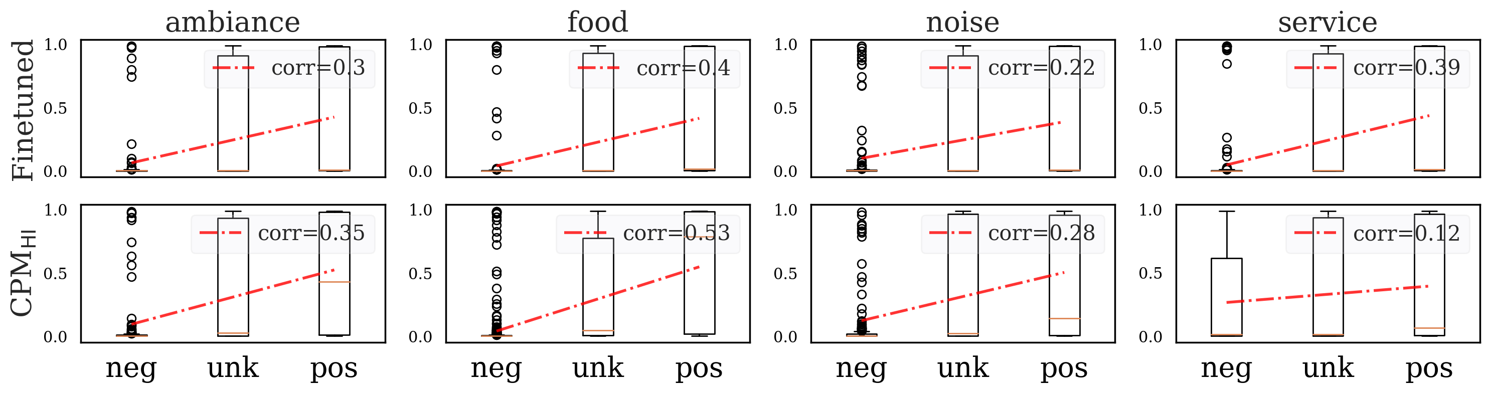
(d) Visualization for debiasing the service concept.

Figure 5: Debiasing visualizations for different concepts of a $\text{CPM{}}_{\text{HI{}}}$ with BERT model architecture. Individual plots are correlation plots between concept labels of a concept and the overall sentence sentiment label.

A.10 Learning Dynamics

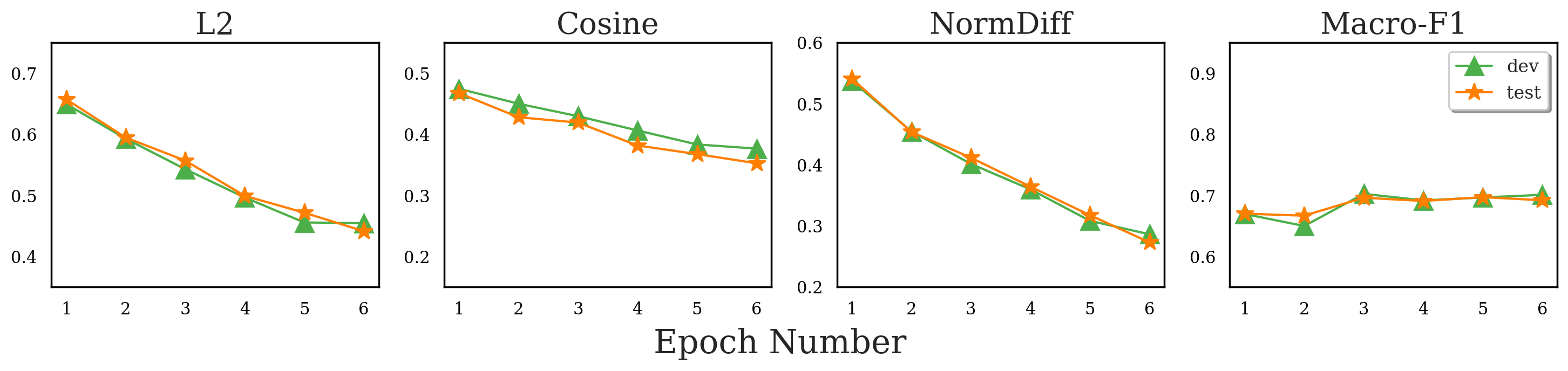
Figure 6: CEBaB scores measured in three different metrics on the dev and the test sets for a $\text{CPM{}}_{\text{HI}}{}$ with the BERT architectures for different training epochs. Task performance as Macro-F1 score is reported.

Figure 6 shows three different metrics measured on the dev and the test sets for a $\text{CPM{}}_{\text{HI}}$ trained for the BERT model architecture as an example. Since we use $\text{COS}_{\texttt{ICaCE}}$ on the dev set to early stop our training process, we find our $\text{CPM{}}_{\text{HI}}$ reaches a local minimum on $\text{COS}_{\texttt{ICaCE}}$ while $\text{L2}_{\texttt{ICaCE}}$ and $\text{NormDiff}_{\texttt{ICaCE}}$ are still trending downward. This suggests future research may need to choose desired metrics to optimize for during training, for early stopping to reach the best performing model.

Epoch	Predicted	Concept	Score	Word Importance
1	neutral	ambiance	$-0.17$	[CLS]themusicwastooloud,andthedecorationsweretaste##less,buttheyhadfriendlywaiter##sanddeliciouspasta[SEP]
		food	$+0.66$	[CLS]themusicwastooloud,andthedecorationsweretaste##less,buttheyhadfriendlywaiter##sanddeliciouspasta[SEP]
		noise	$-0.32$	[CLS]themusicwastooloud,andthedecorationsweretaste##less,buttheyhadfriendlywaiter##sanddeliciouspasta[SEP]
		service	$+0.05$	[CLS]themusicwastooloud,andthedecorationsweretaste##less,buttheyhadfriendlywaiter##sanddeliciouspasta[SEP]
2	neutral	ambiance	$-0.25$	[CLS]themusicwastooloud,andthedecorationsweretaste##less,buttheyhadfriendlywaiter##sanddeliciouspasta[SEP]
		food	$+1.54$	[CLS]themusicwastooloud,andthedecorationsweretaste##less,buttheyhadfriendlywaiter##sanddeliciouspasta[SEP]
		noise	$-0.24$	[CLS]themusicwastooloud,andthedecorationsweretaste##less,buttheyhadfriendlywaiter##sanddeliciouspasta[SEP]
		service	$+0.02$	[CLS]themusicwastooloud,andthedecorationsweretaste##less,buttheyhadfriendlywaiter##sanddeliciouspasta[SEP]
3	neutral	ambiance	$-0.49$	[CLS]themusicwastooloud,andthedecorationsweretaste##less,buttheyhadfriendlywaiter##sanddeliciouspasta[SEP]
		food	$+1.52$	[CLS]themusicwastooloud,andthedecorationsweretaste##less,buttheyhadfriendlywaiter##sanddeliciouspasta[SEP]
		noise	$-0.97$	[CLS]themusicwastooloud,andthedecorationsweretaste##less,buttheyhadfriendlywaiter##sanddeliciouspasta[SEP]
		service	$+0.49$	[CLS]themusicwastooloud,andthedecorationsweretaste##less,buttheyhadfriendlywaiter##sanddeliciouspasta[SEP]
4	neutral	ambiance	$-0.69$	[CLS]themusicwastooloud,andthedecorationsweretaste##less,buttheyhadfriendlywaiter##sanddeliciouspasta[SEP]
		food	$+1.41$	[CLS]themusicwastooloud,andthedecorationsweretaste##less,buttheyhadfriendlywaiter##sanddeliciouspasta[SEP]
		noise	$-1.92$	[CLS]themusicwastooloud,andthedecorationsweretaste##less,buttheyhadfriendlywaiter##sanddeliciouspasta[SEP]
		service	$+1.14$	[CLS]themusicwastooloud,andthedecorationsweretaste##less,buttheyhadfriendlywaiter##sanddeliciouspasta[SEP]
5	neutral	ambiance	$-0.77$	[CLS]themusicwastooloud,andthedecorationsweretaste##less,buttheyhadfriendlywaiter##sanddeliciouspasta[SEP]
		food	$+1.25$	[CLS]themusicwastooloud,andthedecorationsweretaste##less,buttheyhadfriendlywaiter##sanddeliciouspasta[SEP]
		noise	$-1.63$	[CLS]themusicwastooloud,andthedecorationsweretaste##less,buttheyhadfriendlywaiter##sanddeliciouspasta[SEP]
		service	$+1.28$	[CLS]themusicwastooloud,andthedecorationsweretaste##less,buttheyhadfriendlywaiter##sanddeliciouspasta[SEP]
6	neutral	ambiance	$-0.66$	[CLS]themusicwastooloud,andthedecorationsweretaste##less,buttheyhadfriendlywaiter##sanddeliciouspasta[SEP]
		food	$+0.62$	[CLS]themusicwastooloud,andthedecorationsweretaste##less,buttheyhadfriendlywaiter##sanddeliciouspasta[SEP]
		noise	$-0.90$	[CLS]themusicwastooloud,andthedecorationsweretaste##less,buttheyhadfriendlywaiter##sanddeliciouspasta[SEP]
		service	$+2.14$	[CLS]themusicwastooloud,andthedecorationsweretaste##less,buttheyhadfriendlywaiter##sanddeliciouspasta[SEP]
$\text{CPM{}}_{\text{HI}}$	neutral	ambiance	$-0.61$	[CLS]themusicwastooloud,andthedecorationsweretaste##less,buttheyhadfriendlywaiter##sanddeliciouspasta[SEP]
		food	$-0.88$	[CLS]themusicwastooloud,andthedecorationsweretaste##less,buttheyhadfriendlywaiter##sanddeliciouspasta[SEP]
		noise	$-1.34$	[CLS]themusicwastooloud,andthedecorationsweretaste##less,buttheyhadfriendlywaiter##sanddeliciouspasta[SEP]
		service	$+1.75$	[CLS]themusicwastooloud,andthedecorationsweretaste##less,buttheyhadfriendlywaiter##sanddeliciouspasta[SEP]

Table 11: Visualizations of word importance scores using Integrated Gradient (IG), using the same methods as in Table 4 and Table 10.

Table 11 visualizations of word importance scores using our version of Integrated Gradient (IG). Different from Table 4 and Table 10, which show the visualizations of our optimized model, we show a per-epoch result for for $\text{CPM{}}_{\text{HI}}$, followed with our best model appended at the end. Our results suggest that early checkpoints in the training process focus at drastically different input words comparing to later checkpoints, though all models predict neutral for this given sentence. In addition, gradient aggregations over input words are rather stable towards the end the training. More importantly, $\text{CPM{}}_{\text{HI}}$ learns how to highlight words that are semantically related to each concept gradually. For instance, we can see a clear trend of emphasising the word “decorations” for the ambiance concept throughout the training process. This suggests that our training procedure induces causally motivated gradients over input words gradually through the training process.

References

- Abraham et al. (2022) Eldar David Abraham, Karel D’Oosterlinck, Amir Feder, Yair Ori Gat, Atticus Geiger, Christopher Potts, Roi Reichart, and Zhengxuan Wu. CEBaB: Estimating the causal effects of real-world concepts on NLP model behavior. Advances in Neural Information Processing Systems, 2022. URL https://arxiv.org/abs/2205.14140.
- Amodei et al. (2016) Dario Amodei, Chris Olah, Jacob Steinhardt, Paul Christiano, John Schulman, and Dan Mané. Concrete problems in AI safety. , 2016. URL http://arxiv.org/abs/1606.06565.
- Ban et al. (2022) Pangbo Ban, Yifan Jiang, Tianran Liu, and Shane Steinert-Threlkeld. Testing pre-trained language models’ understanding of distributivity via causal mediation analysis. arXiv:2209.04761, 2022. URL https://arxiv.org/abs/2209.04761.
- Binder et al. (2016) Alexander Binder, Grégoire Montavon, Sebastian Lapuschkin, Klaus-Robert Müller, and Wojciech Samek. Layer-wise relevance propagation for neural networks with local renormalization layers. In International Conference on Artificial Neural Networks, 2016. URL https://doi.org/10.1007/978-3-319-44781-0_8.
- Brown et al. (2020) Tom Brown, Benjamin Mann, Nick Ryder, Melanie Subbiah, Jared D Kaplan, Prafulla Dhariwal, Arvind Neelakantan, Pranav Shyam, Girish Sastry, Amanda Askell, et al. Language models are few-shot learners. Advances in Neural Information Processing Systems, 2020. URL https://proceedings.neurips.cc/paper/2020/file/1457c0d6bfcb4967418bfb8ac142f64a-Paper.pdf.
- Buitinck et al. (2013) Lars Buitinck, Gilles Louppe, Mathieu Blondel, Fabian Pedregosa, Andreas Mueller, Olivier Grisel, Vlad Niculae, Peter Prettenhofer, Alexandre Gramfort, Jaques Grobler, Robert Layton, Jake VanderPlas, Arnaud Joly, Brian Holt, and Gaël Varoquaux. API design for machine learning software: Experiences from the scikit-learn project. In ECML PKDD Workshop: Languages for Data Mining and Machine Learning, 2013. URL https://hal.inria.fr/hal-00856511.
- Clark et al. (2019) Kevin Clark, Urvashi Khandelwal, Omer Levy, and Christopher D. Manning. What does BERT look at? An analysis of BERT’s attention. In Proceedings of the 2019 ACL Workshop BlackboxNLP: Analyzing and Interpreting Neural Networks for NLP, Florence, Italy, 2019. URL https://www.aclweb.org/anthology/W19-4828.
- Conneau et al. (2018) Alexis Conneau, German Kruszewski, Guillaume Lample, Loïc Barrault, and Marco Baroni. What you can cram into a single $&!#* vector: Probing sentence embeddings for linguistic properties. In Proceedings of the 56th Annual Meeting of the Association for Computational Linguistics, Melbourne, Australia, 2018. URL https://www.aclweb.org/anthology/P18-1198.
- De Cao et al. (2021) Nicola De Cao, Leon Schmid, Dieuwke Hupkes, and Ivan Titov. Sparse interventions in language models with differentiable masking. arxiv:2112.06837, 2021. URL https://arxiv.org/abs/2112.06837.
- Devlin et al. (2019) Jacob Devlin, Ming-Wei Chang, Kenton Lee, and Kristina Toutanova. BERT: Pre-training of deep bidirectional transformers for language understanding. In Proceedings of the 2019 Conference of the North American Chapter of the Association for Computational Linguistics: Human Language Technologies, Minneapolis, Minnesota, 2019. URL https://www.aclweb.org/anthology/N19-1423.
- Ehsan et al. (2021) Upol Ehsan, Q Vera Liao, Michael Muller, Mark O Riedl, and Justin D Weisz. Expanding explainability: Towards social transparency in AI systems. In Proceedings of the 2021 CHI Conference on Human Factors in Computing Systems, 2021. URL https://dl.acm.org/doi/pdf/10.1145/3411764.3445188.
- Elazar et al. (2021) Yanai Elazar, Shauli Ravfogel, Alon Jacovi, and Yoav Goldberg. Amnesic probing: Behavioral explanation with amnesic counterfactuals. Transactions of the Association for Computational Linguistics, 2021. URL https://direct.mit.edu/tacl/article/doi/10.1162/tacl_a_00359/98091/Amnesic-Probing-Behavioral-Explanation-with.
- Feder et al. (2020) Amir Feder, Nadav Oved, Uri Shalit, and Roi Reichart. CausaLM: Causal model explanation through counterfactual language models. Computational Linguistics, 2020. URL https://aclanthology.org/2021.cl-2.13.
- Geiger et al. (2020) Atticus Geiger, Kyle Richardson, and Christopher Potts. Neural natural language inference models partially embed theories of lexical entailment and negation. In Proceedings of the Third BlackboxNLP Workshop on Analyzing and Interpreting Neural Networks for NLP, 2020. URL https://aclanthology.org/2020.blackboxnlp-1.16.
- Geiger et al. (2021) Atticus Geiger, Hanson Lu, Thomas Icard, and Christopher Potts. Causal abstractions of neural networks. Advances in Neural Information Processing Systems, 2021. URL https://proceedings.neurips.cc/paper/2021/file/4f5c422f4d49a5a807eda27434231040-Paper.pdf.
- Geiger et al. (2022) Atticus Geiger, Zhengxuan Wu, Hanson Lu, Josh Rozner, Elisa Kreiss, Thomas Icard, Noah Goodman, and Christopher Potts. Inducing causal structure for interpretable neural networks. In International Conference on Machine Learning, 2022. URL https://proceedings.mlr.press/v162/geiger22a.html.
- Goodman & Flaxman (2017) Bryce Goodman and Seth Flaxman. European Union regulations on algorithmic decision-making and a “right to explanation”. AI Magazine, 2017. URL http://arxiv.org/abs/1606.08813.
- Goyal et al. (2019) Yash Goyal, Ziyan Wu, Jan Ernst, Dhruv Batra, Devi Parikh, and Stefan Lee. Counterfactual visual explanations. In International Conference on Machine Learning, 2019. URL http://proceedings.mlr.press/v97/goyal19a.html.
- Guidotti et al. (2018) Riccardo Guidotti, Anna Monreale, Salvatore Ruggieri, Franco Turini, Fosca Giannotti, and Dino Pedreschi. A survey of methods for explaining black box models. ACM computing surveys (CSUR), 2018. URL https://dl.acm.org/doi/abs/10.1145/3236009.
- Hardt et al. (2016) Moritz Hardt, Eric Price, and Nati Srebro. Equality of opportunity in supervised learning. In Advances in Neural Information Processing Systems. Curran Associates, Inc., 2016. URL https://proceedings.neurips.cc/paper/2016/file/9d2682367c3935defcb1f9e247a97c0d-Paper.pdf.
- Hinton et al. (2015) Geoffrey Hinton, Oriol Vinyals, Jeff Dean, et al. Distilling the knowledge in a neural network. NeurIPS Deep Learning and Representation Learning Workshop, 2015. URL https://arxiv.org/abs/1503.02531.
- Hochreiter & Schmidhuber (1997) Sepp Hochreiter and Jürgen Schmidhuber. Long short-term memory. Neural Computation, 1997. URL https://ieeexplore.ieee.org/abstract/document/6795963.
- Holland (1986) Paul W Holland. Statistics and causal inference. Journal of the American statistical Association, 1986. URL https://www.tandfonline.com/doi/abs/10.1080/01621459.1986.10478354.
- Jacovi & Goldberg (2020) Alon Jacovi and Yoav Goldberg. Towards faithfully interpretable NLP systems: How should we define and evaluate faithfulness? In Proceedings of the 58th Annual Meeting of the Association for Computational Linguistics, 2020. URL https://aclanthology.org/2020.acl-main.386.
- Jakesch et al. (2019) Maurice Jakesch, Megan French, Xiao Ma, Jeffrey T Hancock, and Mor Naaman. AI-mediated communication: How the perception that profile text was written by AI affects trustworthiness. In Proceedings of the 2019 CHI Conference on Human Factors in Computing Systems, 2019. URL https://dl.acm.org/doi/abs/10.1145/3290605.3300469.
- Kim (2015) Been Kim. Interactive and Interpretable Machine Learning Models for Human Machine Collaboration. PhD thesis, Massachusetts Institute of Technology, 2015. URL https://dspace.mit.edu/handle/1721.1/98680.
- Kim et al. (2018) Been Kim, Martin Wattenberg, Justin Gilmer, Carrie Cai, James Wexler, Fernanda Viegas, and Rory Sayres. Interpretability beyond feature attribution: Quantitative testing with concept activation vectors (TCAV). In International Conference on Machine Learning, 2018. URL http://proceedings.mlr.press/v80/kim18d.html.
- Kleinberg et al. (2017) Jon Kleinberg, Sendhil Mullainathan, and Manish Raghavan. Inherent trade-offs in the fair determination of risk scores. In 8th Innovations in Theoretical Computer Science Conference, 2017. URL http://drops.dagstuhl.de/opus/volltexte/2017/8156.
- Koh et al. (2020) Pang Wei Koh, Thao Nguyen, Yew Siang Tang, Stephen Mussmann, Emma Pierson, Been Kim, and Percy Liang. Concept bottleneck models. In International Conference on Machine Learning, 2020. URL https://proceedings.mlr.press/v119/koh20a.html.
- Künzel et al. (2019) Sören R Künzel, Jasjeet S Sekhon, Peter J Bickel, and Bin Yu. Metalearners for estimating heterogeneous treatment effects using machine learning. Proceedings of the National Academy of Sciences, 2019.
- Lipton (2018) Zachary C. Lipton. The mythos of model interpretability. Communications of the ACM, 2018. URL https://doi.org/10.1145/3233231.
- Liu et al. (2019) Yinhan Liu, Myle Ott, Naman Goyal, Jingfei Du, Mandar Joshi, Danqi Chen, Omer Levy, Mike Lewis, Luke Zettlemoyer, and Veselin Stoyanov. RoBERTa: A robustly optimized BERT pretraining approach. , 2019. URL http://arxiv.org/abs/1907.11692.
- Lovering & Pavlick (2022) Charles Lovering and Ellie Pavlick. Unit testing for concepts in neural networks. arXiv preprint arXiv:2208.10244, 2022.
- Manning et al. (2020) Christopher D. Manning, Kevin Clark, John Hewitt, Urvashi Khandelwal, and Omer Levy. Emergent linguistic structure in artificial neural networks trained by self-supervision. Proceedings of the National Academy of Sciences, 2020. URL https://www.pnas.org/content/117/48/30046.
- Mehrabi et al. (2021) Ninareh Mehrabi, Fred Morstatter, Nripsuta Saxena, Kristina Lerman, and Aram Galstyan. A survey on bias and fairness in machine learning. ACM Computing Surveys (CSUR), 2021. URL https://dl.acm.org/doi/abs/10.1145/3457607.
- Molnar (2020) Christoph Molnar. Interpretable Machine Learning. , 2020.
- Otte (2013) Clemens Otte. Safe and interpretable machine learning: A methodological review. In Computational Intelligence in Intelligent Data Analysis, 2013. URL https://link.springer.com/chapter/10.1007/978-3-642-32378-2_8.
- Paszke et al. (2019) Adam Paszke, Sam Gross, Francisco Massa, Adam Lerer, James Bradbury, Gregory Chanan, Trevor Killeen, Zeming Lin, Natalia Gimelshein, Luca Antiga, et al. Pytorch: An imperative style, high-performance deep learning library. Advances in Neural Information Processing Systems, 2019.
- Pearl (2019) Judea Pearl. The limitations of opaque learning machines. Possible Minds: Twenty-Five Ways of Looking at AI, 2019. URL https://ftp.cs.ucla.edu/pub/stat_ser/r489.pdf.
- Pennington et al. (2014) Jeffrey Pennington, Richard Socher, and Christopher Manning. GloVe: Global vectors for word representation. In Proceedings of the 2014 Conference on Empirical Methods in Natural Language Processing (EMNLP), 2014. URL https://aclanthology.org/D14-1162.
- Radford et al. (2019) Alec Radford, Jeffrey Wu, Rewon Child, David Luan, Dario Amodei, and Ilya Sutskever. Language models are unsupervised multitask learners. OpenAI blog, 2019. URL https://cdn.openai.com/better-language-models/language_models_are_unsupervised_multitask_learners.pdf.
- Ravfogel et al. (2020) Shauli Ravfogel, Yanai Elazar, Hila Gonen, Michael Twiton, and Yoav Goldberg. Null it out: Guarding protected attributes by iterative nullspace projection. In Proceedings of the 58th Annual Meeting of the Association for Computational Linguistics, 2020. URL https://aclanthology.org/2020.acl-main.647.
- Ribeiro et al. (2016) Marco Tulio Ribeiro, Sameer Singh, and Carlos Guestrin. "Why Should I Trust You?": Explaining the predictions of any classifier. In Proceedings of the 22nd ACM SIGKDD International Conference on Knowledge Discovery and Data Mining, San Francisco California USA, 2016. URL https://dl.acm.org/doi/10.1145/2939672.2939778.
- Saphra & Lopez (2019) Naomi Saphra and Adam Lopez. Understanding learning dynamics of language models with SVCCA. In Proceedings of the 2019 Conference of the North American Chapter of the Association for Computational Linguistics: Human Language Technologies, 2019. URL https://www.aclweb.org/anthology/N19-1329.
- Shrikumar et al. (2017) Avanti Shrikumar, Peyton Greenside, and Anshul Kundaje. Learning Important Features through Propagating Activation Differences. In International Conference on Machine Learning, 2017. URL http://proceedings.mlr.press/v70/shrikumar17a.
- Soulos et al. (2020) Paul Soulos, R. Thomas McCoy, Tal Linzen, and Paul Smolensky. Discovering the compositional structure of vector representations with role learning networks. In Proceedings of the Third BlackboxNLP Workshop on Analyzing and Interpreting Neural Networks for NLP, Online, 2020. URL https://aclanthology.org/2020.blackboxnlp-1.23.
- Springenberg et al. (2014) Jost Springenberg, Alexey Dosovitskiy, Thomas Brox, and Martin Riedmiller. Striving for simplicity: the all convolutional net. CoRR, 12 2014. URL https://arxiv.org/abs/1412.6806.
- Sundararajan et al. (2017) Mukund Sundararajan, Ankur Taly, and Qiqi Yan. Axiomatic attribution for deep networks. In Proceedings of the 34th International Conference on Machine Learning - Volume 70, 2017. URL http://proceedings.mlr.press/v70/sundararajan17a.html.
- Tenney et al. (2019) Ian Tenney, Dipanjan Das, and Ellie Pavlick. BERT rediscovers the classical NLP pipeline. In Proceedings of the 57th Annual Meeting of the Association for Computational Linguistics, 2019. URL https://www.aclweb.org/anthology/P19-1452.
- Vaswani et al. (2017) Ashish Vaswani, Noam Shazeer, Niki Parmar, Jakob Uszkoreit, Llion Jones, Aidan N Gomez, Łukasz Kaiser, and Illia Polosukhin. Attention is all you need. In Advances in Neural Information Processing Systems 30. , 2017. URL http://papers.nips.cc/paper/7181-attention-is-all-you-need.pdf.
- Verma et al. (2020) Sahil Verma, John Dickerson, and Keegan Hines. Counterfactual explanations for machine learning: A review. , 2020. URL https://arxiv.org/abs/2010.10596.
- Vig et al. (2020) Jesse Vig, Sebastian Gehrmann, Yonatan Belinkov, Sharon Qian, Daniel Nevo, Yaron Singer, and Stuart M. Shieber. Investigating gender bias in language models using causal mediation analysis. In Advances in Neural Information Processing Systems, 2020. URL https://proceedings.neurips.cc/paper/2020/hash/92650b2e92217715fe312e6fa7b90d82-Abstract.html.
- Wolf et al. (2019) Thomas Wolf, Lysandre Debut, Victor Sanh, Julien Chaumond, Clement Delangue, Anthony Moi, Pierric Cistac, Tim Rault, Rémi Louf, Morgan Funtowicz, et al. Huggingface’s transformers: State-of-the-art natural language processing. , 2019. URL https://arxiv.org/abs/1910.03771.
- Wu et al. (2021) Tongshuang Wu, Marco Tulio Ribeiro, Jeffrey Heer, and Daniel Weld. Polyjuice: Generating counterfactuals for explaining, evaluating, and improving models. In Proceedings of the 59th Annual Meeting of the Association for Computational Linguistics and the 11th International Joint Conference on Natural Language Processing, 2021.
- Yeh et al. (2020) Chih-Kuan Yeh, Been Kim, Sercan Arik, Chun-Liang Li, Tomas Pfister, and Pradeep Ravikumar. On completeness-aware concept-based explanations in deep neural networks. Advances in Neural Information Processing Systems, 2020. URL https://proceedings.neurips.cc/paper/2020/file/ecb287ff763c169694f682af52c1f309-Paper.pdf.
- Zeiler & Fergus (2014) Matthew D. Zeiler and Rob Fergus. Visualizing and understanding convolutional networks. In David Fleet, Tomas Pajdla, Bernt Schiele, and Tinne Tuytelaars (eds.), European Conference on Computer Vision, 2014. URL https://link.springer.com/chapter/10.1007/978-3-319-10590-1_53.