Compositional Score Modeling for Simulation-Based Inference

Abstract

Neural Posterior Estimation methods for simulation-based inference can be ill-suited for dealing with posterior distributions obtained by conditioning on multiple observations, as they tend to require a large number of simulator calls to learn accurate approximations. In contrast, Neural Likelihood Estimation methods can handle multiple observations at inference time after learning from individual observations, but they rely on standard inference methods, such as MCMC or variational inference, which come with certain performance drawbacks. We introduce a new method based on conditional score modeling that enjoys the benefits of both approaches. We model the scores of the (diffused) posterior distributions induced by individual observations, and introduce a way of combining the learned scores to approximately sample from the target posterior distribution. Our approach is sample-efficient, can naturally aggregate multiple observations at inference time, and avoids the drawbacks of standard inference methods.

1 Introduction

Mechanistic simulators have been developed in a wide range of scientific domains to model complex phenomena (Cranmer et al., 2020). Often, these simulators act as a black box: they are controlled by parameters $\theta$ and can be simulated to produce a synthetic observation $x$. Typically, the parameters $\theta$ need to be inferred from data. In this paper, we consider the Bayesian formulation of this problem: given a prior $p(\theta)$ and a set of i.i.d. observations $x^{o}_{1},\ldots,x^{o}_{n}$, the goal is to approximate the posterior distribution $p(\theta|x^{o}_{1},\ldots,x^{o}_{n})\propto p(\theta)\prod_{i=1}^{n}p(x^{o}_{i}|\theta)$.

Simulators can be easily sampled from, but the distribution over the outputs—the likelihood $p(x|\theta)$—cannot be generally evaluated, as it is implicitly defined. This renders standard inference algorithms that rely on likelihood evaluations, such as Markov chain Monte Carlo (MCMC) or variational inference, inapplicable. Instead, a family of inference methods that rely solely on simulations, known as simulation-based inference (SBI), have been developed for performing inference with these models (Beaumont, 2019).

Approximate Bayesian Computation is a traditional SBI method (Sisson et al., 2018). Its simplest form is based on rejection sampling, while more advanced variants involve adaptations of MCMC (Marjoram et al., 2003) and sequential Monte Carlo (Sisson et al., 2007; Del Moral et al., 2012). While popular, these methods often require many simulator calls to yield accurate approximations, which may be problematic with expensive simulators. Thus, recent work has focused on developing algorithms that yield good approximations using a limited budget of simulator calls.

Neural Posterior Estimation (NPE) is a promising alternative (Papamakarios & Murray, 2016; Lueckmann et al., 2017; Chan et al., 2018). NPE methods train a conditional density estimator $q(\theta|x_{1},\ldots,x_{n})$ to approximate the target posterior, using a dataset built by sampling the prior $p(\theta)$ and the simulator $p(x|\theta)$ multiple times. These methods have shown good performance when approximating posteriors $p(\theta|x^{o})$ conditioned on a single observation $x^{o}$ (i.e. $n=1$) (Lueckmann et al., 2021). However, their efficiency decreases for multiple observations ($n>1$), or when $n$ is not known a priori, as in such cases the simulator needs to be called several times per setting of parameters $\theta$ to generate each training case in the dataset, which is inefficient.

Neural Likelihood Estimation (NLE) (Wood, 2010; Papamakarios et al., 2019; Lueckmann et al., 2019) is a natural alternative when the goal is to approximate posteriors conditioned on multiple observations. NLE methods train a surrogate likelihood $q(x|\theta)$ using samples from $p(x|\theta)$. Then, given observations $x_{1}^{o},\ldots,x_{n}^{o}$, inference is carried out using the surrogate likelihood by standard methods, typically MCMC (Papamakarios et al., 2019; Lueckmann et al., 2019) or variational inference (Wiqvist et al., 2021; Glöckler et al., 2022). In contrast to NPE, NLE methods require a single call to the simulator per training case, and can naturally handle an arbitrary number of i.i.d. observations at inference time. However, their performance is hampered by their reliance on the underlying inference method, which can introduce additional approximation error and extra failure modes, such as struggling with multimodal distributions.

In this work, we aim to develop a method that enjoys most of the benefits of existing approaches while avoiding their drawbacks. That is, we aim for a method that (i) can aggregate an arbitrary number of observations at inference time while requiring a low number of simulator calls per training case; and (ii) avoids the limitations of standard inference methods. To this end, we make use of score modeling (also known as diffusion modeling), which has recently emerged as a powerful approach for modeling distributions (Sohl-Dickstein et al., 2015; Ho et al., 2020; Song & Ermon, 2019). Score-based methods diffuse the target distribution with Gaussian kernels of increasing noise levels, train a score network to model the score (gradient of the log-density) of the resulting densities, and use the trained network to approximately sample the target. They have shown impressive performance, particularly in text-conditional image generation (Nichol et al., 2022; Ramesh et al., 2022).

In principle, one could directly apply conditional score-based methods (i.e., conditional diffusion models) (Ho et al., 2020; Song et al., 2020; Batzolis et al., 2021) to the SBI task, which leads to an approach we call Neural Posterior Score Estimation (NPSE). However, as explained in Section 3.2, this fails to satisfy our desiderata. We address this by proposing a different destructive/forward process to the one typically used by diffusion models. Simply put, we factorize the distribution $p(\theta|x_{1},\ldots,x_{n})$ in terms of the posterior distributions induced by individual observations $p(\theta|x_{i})$, train a conditional score network to approximate the score of (diffused versions of) $p(\theta|x)$ for any single $x$, and propose an algorithm that uses the trained network to approximately sample from the posterior $p(\theta|x^{o}_{1},\ldots,x^{o}_{n})$ for any number of observations $n$. Our method satisfies our desiderata: it can naturally handle sets of observations of arbitrary sizes without increasing the simulation cost, and it avoids the limitations of standard inference methods by using an annealing-style sampling algorithm (Sohl-Dickstein et al., 2015; Song & Ermon, 2019; Ho et al., 2020). We describe our approach, called Factorized Neural Posterior Score Estimation (F-NPSE), in detail in Section 3.

Additionally, a simple analysis suggests that NPSE and F-NPSE should not be seen as independent, but as the two extremes of a spectrum of methods. We present this analysis in Section 3.3, where we also propose a family of approaches, called Partially Factorized Neural Posterior Score Estimation (PF-NPSE), that populates this spectrum.

Finally, Section 5 presents a comprehensive empirical evaluation of the proposed approaches on a range of tasks typically used to evaluate SBI methods (Lueckmann et al., 2021). Our results show that our proposed methods tend to outperform relevant baselines when multiple observations are available at inference time, and that the use of methods in the PF-NPSE family often leads to increased robustness.

2 Preliminaries

2.1 Simulation-based Inference

Neural Posterior Estimation (NPE).

NPE methods use a conditional neural density estimator, typically a normalizing flow (Tabak & Turner, 2013; Rezende & Mohamed, 2015; Winkler et al., 2019), to approximate the target posterior. When observed data consists of a single sample $x^{o}$, the $\psi$-parameterized density estimator $q_{\psi}(\theta|x)$ is trained via maximum likelihood, maximizing $\mathop{\mathbb{E}}_{p(\theta)p(x|\theta)}\log q_{\psi}(\theta|x)$ with respect to $\psi$. Since this expectation is intractable, NPE replaces it with an empirical approximation over a dataset $\{\theta^{i},x^{i}\}_{i=1}^{M}$, where $(\theta^{i},x^{i})\sim p(\theta)p(x|\theta)$. Since the conditional neural density estimator takes as input both $\theta$ and $x$, models $q_{\psi}(\theta|x)$ trained this way provide an amortized approximation to the target posterior distribution: at inference time, $q_{\psi}(\theta|x^{o})$ yields an approximation of $p(\theta|x^{o})$ for any observation $x^{o}$.

The situation changes when we have $n>1$ observations at inference time, since it is often not clear how to combine approximations $q_{\psi}(\theta|x^{o}_{i})\approx p(\theta|x^{o}_{i})$ to get a tractable approximation of $p(\theta|x^{o}_{1},\ldots,x^{o}_{n})$. Instead, the density estimator has to take a set of $n$ observations as conditioning, $q_{\psi}(\theta|x_{1},\ldots,x_{n})$, and training has to be done on samples $(\theta^{i},x_{1}^{i},\ldots,x_{n}^{i})\sim p(\theta)\prod_{j}p(x_{j}|\theta)$ (Chan et al., 2018). While the learned density estimator provides an amortized approximation to the target posterior, this comes at the price of reduced sample efficiency, as generating each training case requires $n$ simulator calls per parameter setting $\theta$.

NPE methods can also be used when the number of observations $n$ is not known a priori (Radev et al., 2020). In such cases the density estimator is trained to handle from $n=1$ to $n_{\max}$ observations. This can be achieved by parameterizing $q_{\psi}(\theta|x_{1},\ldots,x_{n})=q_{\psi}(\theta|h_{\psi}(x_{1},\ldots,x_{n}),n)$ with a permutation-invariant function $h_{\psi}$ (Zaheer et al., 2017), and learning from training cases with a variable number of observations $(n^{i},\theta^{i},x_{1}^{i},\ldots,x^{i}_{n^{i}})\sim\mathcal{U}(n;n_{\max})p(\theta)\prod_{j=1}^{n}p(x_{j}|\theta)$, where $\mathcal{U}(\cdot;n_{\max})$ is the uniform distribution over $\{1,2,\ldots,n_{\max}\}$. Then, at inference time, the density estimator provides an approximation of $p(\theta|x^{o}_{1},\ldots,x^{o}_{n_{o}})$ for any set of observations $x^{o}_{1},\ldots,x^{o}_{n_{o}}$ with cardinality $n_{o}\in\{1,2,\ldots,n_{\max}\}$. This approach requires, on average, $n_{\max}/2$ simulator calls per training case.

Neural Likelihood Estimation (NLE).

Instead of approximating the posterior distribution directly, NLE methods train a surrogate $q_{\psi}(x|\theta)$ for the likelihood $p(x|\theta)$. The surrogate is trained with maximum likelihood on samples $(\theta^{i},x^{i})\sim\tilde{p}(\theta)p(x|\theta)$, where $\tilde{p}(\theta)$ is a proposal distribution with sufficient coverage, which can in the simplest case default to the prior. Then, given an arbitrary set of i.i.d. observations $x_{1}^{o},\ldots,x_{n}^{o}$, inference is carried out by running MCMC or variational inference on the approximate target

$$p(\theta)\prod_{i=1}^{n}q_{\psi}(x_{i}^{o}|\theta),$$ (1)

obtained by replacing the individual likelihoods $p(x_{i}^{o}|\theta)$ in the exact posterior expression $p(\theta|x_{1}^{o},\ldots,x_{n}^{o})\propto p(\theta)\prod_{i=1}^{n}p(x_{i}^{o}|\theta)$ by the learned approximation $q_{\psi}(x_{i}^{o}|\theta)$.

A key benefit of NLE is the ability to aggregate multiple observations at inference time, while only training on single-observation/parameter pairs. This is achieved by exploiting the posterior’s factorization in terms of the individual likelihoods in Equation 1. However, the reliance on MCMC or variational inference can negatively impact NLE’s performance, as it introduces additional approximation error and potential failure modes. For instance, a failure mode often reported for NLE (e.g. by Greenberg et al., 2019) involves its inability to robustly handle multimodality (we also observe this in our empirical evaluation in Section 5).

Neural Ratio Estimation (NRE).

Prior work has proposed to learn likelihood ratios (Pham et al., 2014; Cranmer et al., 2015) instead of the likelihood, and to use the learned ratios to perform inference. This approach retains NLE’s ability to aggregate multiple observations at inference time while training on single-observation/parameter pairs, and may be more convenient than NLE when learning the full likelihood is hard, e.g. when observations are high-dimensional. However, NRE methods still rely on standard inference techniques, which can hurt their performance.

2.2 Conditional Score-based Generative Modeling

This section introduces conditional score-based methods for generative modeling, the main tool behind our approach. The goal of conditional generative modeling is to learn an approximation to a distribution $p(\theta|c)$, for some conditioning variable $c$, given samples $(\theta,c)\sim p(\theta,c)$, which is the problem SBI methods need to solve. Methods based on score modeling have shown impressive performance for this task (Dhariwal & Nichol, 2021; Ho & Salimans, 2022; Ramesh et al., 2022; Saharia et al., 2022a). They define a sequence of densities $p_{0}(\theta|c),\ldots,p_{T}(\theta|c)$ by diffusing the target $p(\theta|c)$ with increasing levels of Gaussian noise, learn the scores of each density in the sequence via denoising score matching (Hyvärinen & Dayan, 2005; Vincent, 2011), and use variants of annealed Langevin dynamics (Roberts & Tweedie, 1996; Welling & Teh, 2011) with the learned scores to approximately sample from the target distribution.

Specifically, given $0\approx\gamma_{T}<\gamma_{T-1}<\cdots<\gamma_{1}<1$ and the corresponding Gaussian diffusion kernels $p_{t}(\theta|\theta^{\prime})=\mathcal{N}(\theta|\sqrt{\gamma_{t}}\,\theta^{\prime},(1-\gamma_{t})I)$, the sequence of densities used by score-based methods is typically defined as

$$\begin{split}\textstyle p_{0}(\theta|c)&=p(\theta|c)\\ p_{t}(\theta|c)&=\int d\theta^{\prime}\,p(\theta^{\prime}|c)p_{t}(\theta|\theta^{\prime}),\end{split}$$ (2)

for $t=1,\ldots,T$. Since $\gamma_{T}\approx 0$, this sequence can be seen as gradually bridging between the tractable reference $\mathcal{N}(\theta|0,I)\approx p_{T}(\theta)$ and the target $p(\theta|c)=p_{0}(\theta|c)$. Score-based methods then train a score network $s_{\psi}(\theta,t,c)$ parameterized by $\psi$ to approximate the scores of these densities, $\nabla_{\theta}\log p_{t}(\theta|c)$, by minimizing the denoising score matching objective (Hyvärinen & Dayan, 2005; Vincent, 2011)

$$\sum_{t=1}^{T-1}\mathop{\mathbb{E}}_{p(c,\theta^{\prime})p_{t}(\theta|\theta^{\prime})}\left[\lambda(t)\left\|s_{\psi}(\theta,t,c)-\nabla_{\theta}\log p_{t}(\theta|\theta^{\prime})\right\|^{2}\right],$$ (3)

where $\lambda(t)$ is some non-negative weighting function (Ho et al., 2020; Song et al., 2021). Finally, the learned score network is used to approximately sample the target using annealed Langevin dynamics, as shown in Algorithm 1. Other, but still related, sampling algorithms can be derived by analysing score-based methods from the perspective of diffusion processes (Ho et al., 2020; Song et al., 2020).

Algorithm 1 Annealed Langevin with learned scores

1:  Input: Score network $s_{\psi}(\theta,t,c)$

2:  Input: Reference $p_{T}(\theta)$, conditioning variable $c$

3:  Input: Number of Langevin steps $L$ and step sizes $\delta_{t}$

4:  $\theta\sim p_{T}(\theta)$ $\triangleright$ Sample reference

5:  for $t=T-1,T-2,\ldots,1$ do

6:     for $s=1,2,\ldots,L$ do

7:        $\eta_{ts}\sim\mathcal{N}(0,I)$ $\triangleright$ Sample noise

8:        $\theta\leftarrow\theta+\frac{\delta_{t}}{2}s_{\psi}(\theta,t,c)+\sqrt{\delta_{t}}\eta_{ts}$ $\triangleright$ Langevin step

9:     end for

10:  end for

3 Score Modeling for SBI

This section presents F-NPSE, our approach to SBI. Our goal is to develop a method that (i) can aggregate an arbitrary number of observations at inference time while requiring a low number of simulator calls per training case; and (ii) avoids the limitations of generic inference methods. We achieve this by building on conditional score modeling, but using a different construction for the bridging densities and reference distribution from the ones typically used. Section 3.1 presents our approach, and Section 3.2 explains why this novel construction is necessary, by showing that the direct application of the score modeling framework to the SBI task (i.e. NPSE), fails to satisfy (i). Finally, Section 3.3 presents PF-NPSE, a family of methods that generalizes F-NPSE and NPSE by interpolating between them.

3.1 Factorized Neural Posterior Score Estimation

F-NPSE builds on the conditional score modeling framework, but with a different construction for the bridging densities and reference distribution. Our construction is based on the factorization of the posterior in terms of the individual observation posteriors (see Appendix C):

$$p(\theta|x_{1},\ldots,x_{n})\propto p(\theta)^{1-n}\prod_{j=1}^{n}p(\theta|x_{j}).$$ (4)

The main idea behind our approach is to define bridging densities that satisfy a similar factorization. To achieve this we propose a sequence indexed by $t=0,\ldots,T$ given by

$$p_{t}^{\mathrm{f}}(\theta|x_{1},\ldots,x_{n})\propto\left(p(\theta)^{1-n}\right)^{\frac{T-t}{T}}\prod_{j=1}^{n}p_{t}(\theta|x_{j}),$$ (5)

where $p_{t}(\theta|x_{j})$ follows Equation 2 with $c=x_{j}$, and the superscript $\mathrm{f}$ is used as an identifier of F-NPSE.

This construction has four key properties. First, the distribution for $t=0$ recovers the target $p(\theta|x_{1},\ldots,x_{n})$. Second, the distribution for $t=T$ approximates a spherical Gaussian $p_{T}^{\mathrm{f}}(\theta|x_{1},\ldots,x_{n})\approx p_{T}(\theta)=\mathcal{N}(\theta|0,\frac{1}{n}I)$, since the prior term vanishes and $p_{T}(\theta|x_{j})\approx\mathcal{N}(\theta|0,I)$, and thus can be used as a tractable reference for the diffusion process. Third, the scores of the resulting densities can be decomposed in terms of the score of the prior (typically available exactly) and the scores of the individual terms $p_{t}(\theta|x_{j})$ as

$$\nabla_{\theta}\log p_{t}^{\mathrm{f}}(\theta|x_{1},\ldots,x_{n})=\\ \frac{(1-n)(T-t)}{T}\nabla_{\theta}\log p(\theta)+\sum_{j=1}^{n}\nabla_{\theta}\log p_{t}(\theta|x_{j}).$$ (6)

And fourth, the scores $\nabla_{\theta}\log p_{t}(\theta|x_{j})$ can all be approximated using a single score network $s_{\psi}(\theta,t,x)$ trained via denoising score matching on samples $(\theta^{i},x^{i})\sim p(\theta)p(x|\theta)$, as explained in Section 2.2.

After training, given i.i.d. observations $x^{o}_{1},\ldots,x^{o}_{n}$, we can approximately sample $p(\theta|x^{o}_{1},\ldots,x^{o}_{n})$ by running Algorithm 1 with the reference $p_{T}(\theta)=\mathcal{N}(\theta|0,\frac{1}{n}I)$, conditioning variable $c=\{x^{o}_{1},\ldots,x^{o}_{n}\}$, and approximate score

$$s_{\psi}(\theta,t,c)=\\ \frac{(1-n)(T-t)}{T}\nabla_{\theta}\log p(\theta)+\sum_{j=1}^{n}s_{\psi}(\theta,t,x^{o}_{j}).$$ (7)

In short, the fact that the bridging densities factorize over individual observations as in Equation 5 allows us to train a score network to approximate the scores of the distributions induced by individual observations, and to aggregate the network’s output for different observations at inference time to sample from the target posterior distribution. Thus, we can aggregate an arbitrary number of observations at inference time while training on samples $(\theta^{i},x^{i})\sim p(\theta)p(x|\theta)$, each one requiring a single simulator call. Additionally, the mass-covering properties of score-based methods (Ho et al., 2020; Song et al., 2021) together with the annealed sampling algorithm avoid the drawbacks of standard inference methods, such as their difficulty with handling multimodality.

As presented, applying F-NPSE to models with constrained priors (e.g. Beta, uniform) requires care, as the densities in Equation 5 are ill-defined outside of the prior’s support. This can be addressed in two ways: (i) reparameterizing the model such that the prior becomes a standard Gaussian; this is often easy to do, and what we do in this work, see Appendix A; or (ii) diffusing the prior and learning the corresponding scores. Concurrent work by Sharrock et al. (2022) explored (ii), obtaining good results.

A potential drawback of F-NPSE is that it might accumulate errors when combining score estimates as in Equation 7, affecting the method’s performance. This drawback is shared by NLE and NRE. We study it empirically in Section 5.

3.2 Direct Application of Conditional Score Modeling

This section introduces NPSE and explains why it fails to satisfy our desiderata, specifically (i). NPSE is a direct application of the score modeling framework to the SBI task. Following Equation 2 with $c=\{x_{1},\ldots,x_{n}\}$, and assuming a fixed number of observations $n$ (relaxed later), NPSE defines a sequence of densities

$$p_{t}(\theta|x_{1},\ldots,x_{n})=\int d\theta^{\prime}\,p(\theta^{\prime}|x_{1},\ldots,x_{n})p_{t}(\theta|\theta^{\prime}),$$ (8)

and trains a score network $s_{\psi}(\theta,t,x_{1},\ldots,x_{n})$ to approximate their scores via denoising score matching. Then, at inference time, given observations $x_{1}^{o},\ldots,x_{n}^{o}$, NPSE uses $s_{\psi}(\theta,t,x^{o}_{1},\ldots,x^{o}_{n})$ to approximately sample $p(\theta|x_{1}^{o},\ldots,x_{1}^{o})$. The approach can be extended to cases where $n$ is not fixed a priori, by parameterizing the score network as $s_{\psi}(\theta,t,x_{1},\ldots,x_{n})=s_{\psi}(\theta,t,h_{\psi}(x_{1},\ldots,x_{n}),n)$ with a permutation-invariant function $h_{\psi}$, and training it on samples $(n^{i},\theta^{i},x_{1}^{i},\ldots,x^{i}_{n^{i}})\sim\mathcal{U}(n;n_{\max})p(\theta)\prod_{j=1}^{n}p(x_{j}|\theta)$.

Unfortunately, NPSE does not satisfy condition (i) outlined above, as it requires specifying the maximum number of observations $n_{\max}$ and needs $n_{\max}/2$ simulator calls per training case on average. Since the scores of the bridging densities defined in Equation 8 do not factorize in terms of the individual observations, the approach taken by F-NPSE, which trains a score network for individual observations and aggregates them at inference time, is not applicable. However, in contrast to F-NPSE, NPSE does not require summing approximations, so it does not accumulate errors.

3.3 Partially Factorized Neural Posterior Score Estimation

We introduced NPSE and F-NPSE, and described their benefits and limitations; F-NPSE is efficient in terms of the number of simulator calls but may accumulate approximation error, while the opposite is true for NPSE. We argue that these two approaches can be seen as the opposite extremes of a family of methods that interpolate between them, achieving different trade-offs between sample efficiency and accumulation of errors. We call these methods Partially Factorized Neural Posterior Score Estimation (PF-NPSE).

PF-NPSE is based on a similar strategy to the one used by F-NPSE, factorizing the target posterior distribution in terms of small subsets of observations instead of individual observations. Specifically, given $m\geq 1$, we partition the set of conditioning variables $\{x_{1},\ldots,x_{n}\}$ into $k=\lceil n/m\rceil$ disjoint subsets of size at most $m$, denoted by $X_{1},\ldots,X_{k}$, and factorize the posterior distribution as

$$p(\theta|x_{1},\ldots,x_{n})\propto p(\theta)^{1-k}\prod_{j=1}^{k}p(\theta|X_{j}).$$ (9)

Then, following the F-NPSE strategy, we define the bridging densities using the diffused versions of each $p(\theta|X_{j})$ as

$$p_{t}^{\mathrm{pf}}(\theta|x_{1},\ldots,x_{n})\propto\left(p(\theta)^{1-k}\right)^{\frac{T-t}{T}}\prod_{j=1}^{k}p_{t}(\theta|X_{j}),$$ (10)

and train a score network $s_{\psi}(\theta,t,X_{j})$ to approximate their scores. Since this network needs to handle input sets $X_{j}$ of sizes varying between $1$ and $m$, we parameterize it using a permutation-invariant function, and train it on samples with a varying number of observations between $1$ and $m$, $(n^{i},\theta^{i},x_{1}^{i},\ldots,x^{i}_{n^{i}})\sim\mathcal{U}(n;m)p(\theta)\prod_{j=1}^{n}p(x_{j}|\theta)$.

At inference time, given observations $x_{1}^{o},\ldots,x_{n}^{o}$, the method approximately samples the target $p(\theta|x^{o}_{1},\ldots,x^{o}_{n})$ by partitioning the observations into subsets $X^{o}_{1},\ldots,X^{o}_{k}$ and running annealed Langevin dynamics (Algorithm 1) with $c=\{X^{o}_{1},\ldots,X^{o}_{k}\}$ and the approximate score

$$s_{\psi}(\theta,t,c)=\\ \frac{(1-n)(T-t)}{T}\nabla_{\theta}\log p(\theta)+\sum_{j=1}^{k}s_{\psi}(\theta,t,X^{o}_{j}).$$ (11)

The value of $m$ controls the trade-off between sample efficiency and error accumulation: for a given $m$, the method gets an approximate score by adding $k=\lceil n/m\rceil$ terms as in Equation 11, and requires on average $m/2$ simulator calls per training case. Therefore, low values of $m$ yield methods closer to F-NPSE, while larger values yield methods closer to NPSE. In fact, we recover F-NPSE for $m=1$ and NPSE for $m=n_{\max}$. This motivates finding the value of $m$ that achieves the best trade-off. We investigate this empirically in Section 5, where we observe that using low values of $m$ (greater than 1) often yields best results.

4 Related Work

Conditional score modeling has been used in many domains, including image super-resolution (Saharia et al., 2022b; Li et al., 2022), conditional image generation (Batzolis et al., 2021), and time series imputation (Tashiro et al., 2021). Concurrently with this work Sharrock et al. (2022) also studied its application for SBI, proposing a method akin to NPSE (they introduced the name NPSE, which we adopt here for consistency). Unlike our work that shows how NPSE can be extended to accommodate multiple observations, Sharrock et al. (2022) focus on the single-observation case and develop a sequential version of NPSE, which divides the learning process into stages and uses the learned posterior, instead of the prior, to draw parameters $\theta$ at each stage. This sequential approach of using the current posterior approximation to guide future simulations has its roots in the ABC literature (e.g. Sisson et al., 2007; Blum & François, 2010). In the context of neural methods, it was originally proposed for NPE (Papamakarios & Murray, 2016), and was later incorporated into NLE (Papamakarios et al., 2019) and NRE (Hermans et al., 2020b). Previous work has observed that sequential approaches often lead to performance improvements over their non-sequential counterparts (Greenberg et al., 2019; Lueckmann et al., 2021) and are on par with active-learning methods for parameter selection (Durkan et al., 2018). While we do not explore sequential approaches, we note that F-NPSE and PF-NPSE are compatible with the sequential formulation of Sharrock et al. (2022).

Shi et al. (2022) also studied the use of conditional diffusion models in the context of SBI, with the goal of reducing the number of diffusion steps required to obtain good results. To achieve this they extend the diffusion Schrödinger bridge framework (De Bortoli et al., 2021) to perform conditional simulation. Their approach consists of a sequential training procedure where both the forward and backward processes are trained iteratively using score-matching techniques. They additionally propose to learn an observation-dependent reference $p_{T}(\theta|x)$ for the sampling process, replacing the standard Gaussian. Similarly to Sharrock et al. (2022), they focus on the single observation case.

Finally, previous work by Liu et al. (2022) also proposed to compose diffusion models by adding their scores. However, they generate samples by directly plugging the composed score into the time-reverse diffusion of the noising process, which yields an incorrect sampling method (since the score of the true bridging densities does not follow this additive factorization, as explained in Section 3.2). We address this issue by adopting a different sampler based on annealed Langevin dynamics. This solution was also concurrently proposed by Du et al. (2023), who, among other things, proposed a method to compose diffusion models closely related to F-NPSE.

5 Empirical Evaluation

In this section, we empirically evaluate the proposed methods along with a number of baselines. Sections 5.1, LABEL: and 5.2 show results comparing F-NPSE, PF-NPSE, NPSE, NPE, and NRE. We use 400 noise levels for methods based on score modeling, a normalizing flow with six Real NVP layers (Dinh et al., 2016) for NPE, and the NRE method proposed by Hermans et al. (2020a) with HMC (Neal, 2011). We provide the details for all the methods in Appendix B.

Sections 5.3, LABEL: and 5.4 explore the robustness of F-NPSE and PF-NPSE for different design choices and hyperparameters, including the parameterization for the score network, parameters of the Langevin sampler, and the value of $m$ for PF-NPSE. Unless specified otherwise, each method is given a budget of $10^{4}$ simulator calls, and optimization is carried out using Adam (Kingma & Ba, 2014) with the learning rate of $10^{-4}$ for a maximum of 20k epochs (using 20% of the training data as a validation set for early stopping).

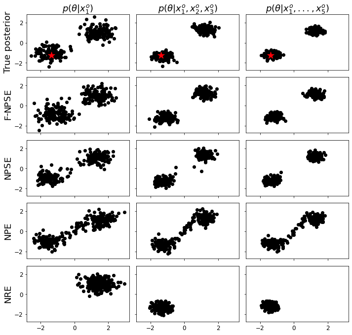
Figure 1: Samples from the approximate posterior obtained by each method. NPE and NPSE use $n_{\max}=5$. The true parameters $\theta$ used to generate $x_{1}^{o},\ldots,x_{5}^{o}$ are shown in red in the first row.

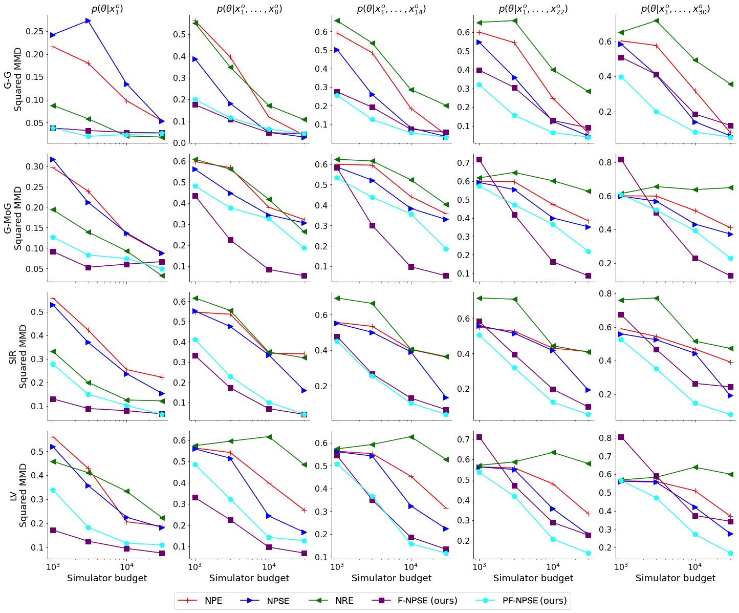
Figure 2: Squared MMD (lower is better) obtained by each method on different tasks. Plots show “Squared MMD” ($y$-axis) vs. “simulator budget used for training” ($x$-axis), and each line corresponds to a different method. Rows correspond to the different models considered (Gaussian/Gaussian, Gaussian/Mixture of Gaussians, SIR, Lotka–Volterra), and columns to the different number of conditioning observations available at inference time (1, 8, 14, 22, 30). We use $n_{\max}=30$ for NPE and NPSE and $m=6$ for PF-NPSE.

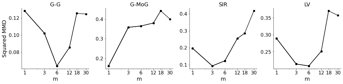
Figure 3: Squared MMD (lower is better) obtained by PF-NPSE when estimating posterior distributions obtained by conditioning on 22 observations. Each plot corresponds to a different task, and shows “Squared MMD” ($y$-axis) vs. “$m$ (used for PF-NPSE)” ($x$-axis).

5.1 Illustrative Multimodal Example

We begin with a qualitative comparison on a 2-dimensional example with a multimodal posterior, where the prior and likelihood are given by $p(\theta)=\mathcal{N}(\theta|0,I)$ and $p(x|\theta)=\frac{1}{2}\mathcal{N}(x|\theta,\frac{I}{2})+\frac{1}{2}\mathcal{N}(x|-\theta,\frac{I}{2})$. We use $n_{\max}=5$ for NPE and NPSE. After training, we sample $\theta\sim p(\theta)$ and $x^{o}_{1},\ldots,x^{o}_{5}\overset{\mathrm{iid}}{\sim}p(x|\theta)$, and use each method to approximate the posterior distribution obtained by conditioning on subsets of $\{x^{o}_{1},\ldots,x^{o}_{5}\}$ of different sizes.

Figure 1 shows that F-NPSE is able to capture both modes well for all subsets of observations considered, despite being trained using a single observation per training case. While NPE and NPSE also perform well, NRE fails to sample both modes, because HMC struggles to mix between modes, which is often an issue with MCMC samplers.

5.2 Systematic Evaluation

We now present a systematic evaluation on four tasks typically used to evaluate SBI methods (Lueckmann et al., 2021), which are described in detail in Appendix A.

Gaussian/Gaussian (G-G). A 10-dimensional model with a Gaussian prior $p(\theta)=\mathcal{N}(\theta|0,I)$ and a Gaussian likelihood $p(x|\theta)=\mathcal{N}(x|\theta,\Sigma)$, with $\Sigma$ set to a diagonal matrix with elements increasing linearly from $0.6$ to $1.4$.

Gaussian/Mixture of Gaussians (G-MoG). A 10-dimensional model with a prior $p(\theta)=\mathcal{N}(\theta|0,I)$ and a mixture of two Gaussians with a shared mean as the likelihood $p(x|\theta)=\frac{1}{2}\mathcal{N}(x|\theta,2.25\Sigma)+\frac{1}{2}\mathcal{N}(x|\theta,\frac{1}{9}\Sigma)$.

Susceptible-Infected-Recovered (SIR). A model used to track the evolution of a disease, modeling the number of individuals in each of three states: susceptible (S), infected (I), and recovered (R) (Harko et al., 2014). The values for the variables S, I, R are governed by a non-linear dynamical system with two parameters, the contact rate and the recovery rate, which must be inferred from noisy observations of the number of individuals in each state at different times.

Lotka–Volterra (LV). A predator-prey model used in ecology to track the evolution of the number of individuals of two interacting species. The model consists of a non-linear dynamical system with four parameters, which must be inferred from noisy observations of the number of individuals of both species at different times.

We compare the methods’ performance for different simulator call budgets $B\in\{10^{3},3\cdot 10^{3},10^{4},3\cdot 10^{4}\}$. We train using learning rates $\{10^{-3},10^{-4}\}$, keeping the one that yields the best validation loss for each method and simulator budget. We use $n_{\max}=30$ for NPE and NPSE and $m=6$ for PF-NPSE. We train each method five times using different random seeds, and for each run we perform the evaluation using six different sets of parameters $\theta\sim p(\theta)$, not shared between runs. After training, we generate observations by drawing $\theta\sim p(\theta)$ and $x_{1}^{o},\ldots,x_{30}^{o}\overset{\mathrm{iid}}{\sim}p(x|\theta)$, and report each method’s performance when approximating the posterior conditioned on subsets of $\{x_{1}^{o},\ldots,x_{30}^{o}\}$ of different sizes. We report the squared Maximum Mean Discrepancy (MMD) (Gretton et al., 2012) between the true posterior distribution and the approximations, using the Gaussian kernel with the scale determined by the median distance heuristic (Ramdas et al., 2015). We also report results using classifier two-sample tests in Section E.1.

We can draw several conclusions from Figure 2, which shows the average results. First, as expected, performance tends to improve for all methods as the simulator call budget is increased. Second, in most cases the top performing method is F-NPSE or PF-NPSE. In fact, PF-NPSE typically outperforms all baselines, and is second to F-NPSE when the number of conditioning observations is low (i.e., $n\leq 10$). The fact that PF-NPSE with $m=6$ often outperforms both F-NPSE and NPSE indicates that neither of the two extremes achieves the best trade-off between sample efficiency and accumulation of errors, and that methods in the spectrum interpolating between them are often preferred. We investigate this more thoroughly in Section 5.3. Finally, while NRE methods can naturally aggregate multiple observations at inference time, they also suffer from accumulation of errors. Results in Figure 2 suggest that F-NPSE and PF-NPSE tend to scale better to large numbers of observations than NRE. We believe this may be due to learning density ratios being a challenging problem, with new methods being actively developed (Rhodes et al., 2020; Choi et al., 2022).

5.3 Optimal Trade-off for PF-NPSE

In this section, we study the performance of PF-NPSE as a function of $m$. As explained in Section 3, the value of $m$ controls the trade-off between sample-efficiency and accumulation of errors. To investigate this trade-off, we fix $n_{\max}=30$ and evaluate PF-NPSE’s performance for different values of $m\in\{1,3,6,12,18,30\}$, which cover the spectrum between F-NPSE and NPSE. Figure 3 shows results for approximating a posterior distribution conditioned on $22$ observations, $x^{o}_{1},\ldots,x^{o}_{22}$ (see Section E.2 for results for different numbers of conditioning observations). We see that the best performance is often achieved using small values of $m$, typically $3$ or $6$, indicating that the methods located at the both ends of the spectrum, F-NPSE and NPSE, are often suboptimal.

5.4 Score Network and Langevin Sampler

We now investigate the robustness of the proposed methods to different design/hyperparameter choices. Specifically, we study the effect of constraining the score network to output a conservative vector field, by taking the score to be the gradient of a scalar-valued network (Salimans & Ho, 2021), and of the choice of the step-size and the number of steps per noise level in the Langevin sampler. We show the results in Sections E.3, LABEL: and E.4. Overall we find that our methods are robust to different choices: Figure 7 shows that using a conservative parameterization for the score network does not have a considerable effect on performance, and Figure 8 shows that PF-NPSE is robust to changes in the Langevin sampler, as long as it performs a sufficient number of steps (typically 5–10) to converge for each noise level.

5.5 Demonstration: Weinberg Simulator

We conclude our evaluation with a demonstration of F-NPSE with the Weinberg simulator, introduced as a benchmark by Louppe et al. (2017). The simulator models high-energy particle collisions, and the goal is to estimate the Fermi constant given observations for the scattering angle. We use the simplified simulator from Cranmer et al. (2017) with a uniform prior $p(\theta)=\mathcal{U}(0,2)$. To evaluate, we fix the parameters $\theta^{*}$ (we consider $\theta^{*}=0.3$ and $\theta^{*}=1.7$), draw $x_{1},\ldots,x_{5}\overset{\mathrm{iid}}{\sim}p(x|\theta^{*})$, and estimate the posteriors $p(\theta|x_{i})$ for $i=1,\ldots,5$ and $p(\theta|x_{1},\ldots,x_{5})$. Figure 4 shows the results. Posteriors conditioned on individual observations and on all five observations are shown in black and red, respectively. As expected, as the number of observations is increased the posterior returned by F-NPSE concentrates around the true parameter value $\theta^{*}$.

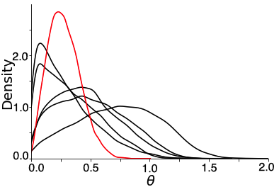
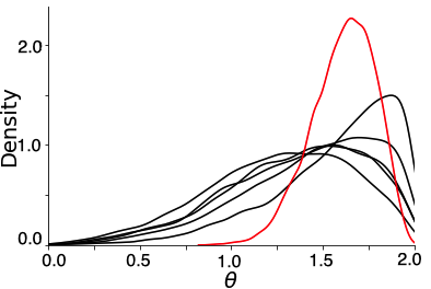
Figure 4: Approximations obtained by F-NPSE on the Weinberg task. Left: $\theta^{*}=0.3$. Right: $\theta^{*}=1.7$. Black lines show approximations obtained for $p(\theta|x_{i})$ for $i=1,\ldots,5$, and red lines shows the approximation for $p(\theta|x_{1},\ldots,x_{5})$. We note that the approximations obtained are constrained to the $[0,2]$ interval (since we reparameterize the model, see Appendix A). The fact that the plots extend beyond these limits is an artifact due to the use of a kernel density estimator.

6 Conclusion and Limitations

We studied the use of conditional score modeling for SBI, proposing several methods that can aggregate information from multiple observations at inference time while requiring a small number of simulator calls to generate each training case. We achieve this using a novel construction for the bridging densities, which allows us to simply aggregate the scores to approximately sample distributions conditioned on multiple observations. We presented an extensive empirical evaluation, which shows promising results for our methods when compared against other approaches able to aggregate an arbitrary number of observations at inference time.

As presented, F-NPSE and PF-NPSE use annealed Langevin dynamics to generate samples. This requires choosing step-sizes $\delta_{t}$, the number of steps $L$ per noise level, and has complexity $\mathcal{O}(LT)$. Appendix D presents an alternative sampling method that can be used with F-NPSE and PF-NPSE which does not use Langevin dynamics, does not have any hyperparameters, and runs in $\mathcal{O}(T)$ steps. While our evaluation of this sampling method shows promising results (Section E.4), we observe that sometimes it underperforms annealed Langevin dynamics. We believe that further study of alternative sampling algorithms is a promising direction for improving F-NPSE and PF-NPSE.

Appendix A Models Used

Multimodal posterior from Section 5.1.

We consider $\theta\in\mathbb{R}^{2}$ and $x\in\mathbb{R}^{2}$, and the prior and likelihood are given by

$$p(\theta)=\mathcal{N}(\theta|0,I)\quad\mbox{and}\quad p(x|\theta)=\frac{1}{2}\mathcal{N}\left(x\big{|}\theta,\frac{I}{2}\right)+\frac{1}{2}\mathcal{N}\left(x\big{|}-\theta,\frac{I}{2}\right).$$ (12)

Gaussian/Gaussian (G-G).

This model was adapted from Lueckmann et al. (2021). We consider $\theta\in\mathbb{R}^{10}$ and $x\in\mathbb{R}^{10}$, and the prior and likelihood given by

$$p(\theta)=\mathcal{N}(\theta|0,I)\quad\mbox{and}\quad p(x|\theta)=\mathcal{N}(x|\theta,\Sigma),$$ (13)

where $\Sigma$ is a diagonal matrix with elements increasing linearly from $0.6$ to $1.4$.

Gaussian/Mixture of Gaussians (G-MoG).

A model similar to this one was originally proposed by Sisson et al. (2007), and was later widely adopted in the SBI literature (Lueckmann et al., 2021). We consider $\theta\in\mathbb{R}^{10}$ and $x\in\mathbb{R}^{10}$, and the prior and likelihood given by

$$p(\theta)=\mathcal{N}(\theta|0,I)\quad\mbox{and}\quad p(x|\theta)=\frac{1}{2}\mathcal{N}\left(x\big{|}\theta,2.25\Sigma\vphantom{\frac{1}{9}}\right)+\frac{1}{2}\mathcal{N}\left(x\big{|}\theta,\frac{1}{9}\Sigma\right),$$ (14)

where $\Sigma$ is a diagonal matrix with elements increasing linearly from $0.6$ to $1.4$.

Susceptible-Infected-Recovered (SIR).

This model describes the transmission of a disease through a population of size $N$, where each individual can be in one of three states: susceptible $S$, infectious $I$, or recovered $R$. We follow the description from Lueckmann et al. (2021, §T9). The model has two parameters, the contact rate $\beta$ and the transmission rate $\gamma$, i.e. $\theta=(\beta,\gamma)$. The simulator numerically simulates the dynamical system given by

$$\begin{split}\frac{\mathrm{d}S}{\mathrm{d}t}&=-\beta\frac{SI}{N}\\ \frac{\mathrm{d}I}{\mathrm{d}t}&=\beta\frac{SI}{N}-\gamma I\\ \frac{\mathrm{d}R}{\mathrm{d}t}&=\gamma I\\ \end{split}$$ (15)

for $160$ seconds, starting from the initial conditions where a single individual is infected and the rest susceptible. The prior over the parameters is given by

$$p(\beta)=\mathrm{LogNormal}(\log(0.4),0.5)\quad\mbox{and}\quad p(\gamma)=\mathrm{LogNormal}(\log(0.125),0.2).$$ (16)

The observations are 10-dimensional vectors corresponding to noisy observations of the number of infected people at 10 evenly-spaced times, $p(x_{i})=\mathcal{B}\left(1000,\frac{I_{i}}{N}\right)$, where $\mathcal{B}$ denotes the binomial distribution and $I_{i}$ the number of infected subjects at the corresponding time.

Lotka–Volterra (LV).

This model describes the evolution of the number of individual of two interacting species, typically a prey and a predator. We follow the description from Lueckmann et al. (2021, §T10). The model has four parameters $\alpha,\beta,\gamma,\delta$. Using $X$ and $Y$ to represent the number of individuals in each species, the simulator numerically simulates the dynamical system given by

$$\begin{split}\frac{\mathrm{d}X}{\mathrm{d}t}&=\alpha X-\beta XY\\ \frac{\mathrm{d}Y}{\mathrm{d}t}&=-\gamma Y+\delta XY.\\ \end{split}$$ (17)

The system is simulated for $20$ seconds, starting from $X_{0}=30$ and $Y_{0}=1$. The prior over the parameters is given by

$$\begin{split}p(\alpha)&=\mathrm{LogNormal}(-0.125,0.5)\\ p(\beta)&=\mathrm{LogNormal}(-3,0.5)\\ p(\gamma)&=\mathrm{LogNormal}(-0.125,0.5)\\ p(\delta)&=\mathrm{LogNormal}(-3,0.5).\end{split}$$ (18)

The observations consist of 20-dimensional vectors corresponding to noisy observations of the number of members of each species at 10 evenly-spaced times, $p(x_{i,X})=\mathrm{LogNormal}(\log(X_{i}),0.1)$ and $p(x_{i,Y})=\mathrm{LogNormal}(\log(Y_{i}),0.1)$.

Weinberg simulator.

This task was originally proposed by Louppe et al. (2017). We use the simplified simulator of Cranmer et al. (2017) with a uniform prior $p(\theta)=\mathcal{U}(0,2)$.

Reparameterizing models.

For all tasks, we reparameterize the models to have a standard Normal prior. This is simple to do with the priors commonly used by these models.

Appendix B Details for each Method

All methods based on denoising diffusion models/score modeling use $T=400$.

B.1 F-NPSE

Our implementation of the score network $s_{\psi}(\theta,t,x)$ used by F-NPSE has three components:

• An MLP with 3 hidden layers that takes $\theta$ as input and outputs an embedding $\theta_{\mathrm{emb}}$,

• An MLP with 3 hidden layers that takes $x$ as input and outputs an embedding $x_{\mathrm{emb}}$,

• An MLP with 3 hidden layers that takes $[\theta_{\mathrm{emb}},x_{\mathrm{emb}},t_{\mathrm{emb}}]$ as input, where $t_{\mathrm{emb}}$ is a positional embedding obtained as described by Vaswani et al. (2017), and outputs an estimate of the score. We parameterize the score in terms of the noise variables (Ho et al., 2020; Luo, 2022).

All MLPs use residual connections (He et al., 2016) and normalization layers (LayerNorm, Ba et al., 2016) throughout.

Running Algorithm 1 to generate samples using the trained score network requires choosing step sizes $\delta_{t}$ and the number of Langevin steps $L$ for each noise level $\gamma_{t}$. We use $L=5$ and $\delta_{t}=0.3\frac{1-\alpha_{t}}{\sqrt{\alpha_{t}}}$, where $\alpha_{1}=\gamma_{1}$ and $\alpha_{t}=\frac{\gamma_{t}}{\gamma_{t-1}}$ for $t=2,\ldots,T-1$.

B.2 PF-NPSE

The architecture for the score network $s_{\psi}(\theta,t,X)$, where $X$ is a set of observations with a number of elements between $1$ and $m$, is similar to the one used for F-NPSE, with two differences. First, each individual observation $x_{i}\in X$ produces and embedding $x_{i,\mathrm{emb}}$, and the final embedding $X_{\mathrm{emb}}$ is obtained by averaging the individual embeddings. Second, the final MLP takes as inputs $[\theta_{\mathrm{emb}},X_{\mathrm{emb}},t_{\mathrm{emb}},n_{\mathrm{emb}}]$, where $n_{\mathrm{emb}}\in\{0,1\}^{m}$ is a 1-hot encoding of the number of observations in the set $X$ (between $1$ and $m$). The Langevin sampler uses the parameters described above.

B.3 NPSE

The architecture is the same as the one for PF-NPSE, with $m=n_{\max}$. Since the method corresponds to a direct application of conditional diffusion models, we use the standard sampler for diffusion models (Ho et al., 2020), which consists of applying $T$ Gaussian transitions, with no tunable parameters.

B.4 NPE

We use an implementation of NPE methods based on flows able to handle sets of observations of any size $n\in\{1,2,\ldots n_{\max}\}$. The flow can be expressed as $q_{\psi}(\theta|x_{1},\ldots,x_{n},n)$. Following Chan et al. (2018) and Radev et al. (2020, §2.4), we use an exchangeable neural network to process the observations $x_{1},\ldots,x_{n}$. Specifically, we use an MLP with 3 hidden layers to generate an embedding $x_{i,\mathrm{emb}}$ for each observation $x_{i}$. We then compute the mean embedding across observations $x_{\mathrm{emb}}=\frac{1}{n}\sum_{i}^{n}x_{i,\mathrm{emb}}$, which we use as input for the conditional flow. Finally, we model the flow $q_{\psi}(\theta|x_{1},\ldots,x_{n},n)=q_{\psi}(\theta|x_{\mathrm{emb}},n_{\mathrm{emb}})$, where $n_{\mathrm{emb}}\in\{0,1\}^{n_{\max}}$ is a 1-hot encoding of the number of observations (between $1$ and $n_{\max}$).

We use 6 Real NVP layers (Dinh et al., 2016) for the flow, each one consisting of MLPs with three hidden layers. As for the other methods, we use residual connections throughout.

B.5 NRE

We use the NRE method proposed by Hermans et al. (2020a). Simply put, the network receives a pair $(\theta,x)$ as input, and is trained to classify whether $(\theta,x)\sim p(\theta,x)$ or $(\theta,x)\sim p(\theta)p(x)$. The optimal classifier learnt this way can be used to compute the ratio $\frac{p(x|\theta)}{p(x)}$. Our classifier consists of three components: two linear layers to compute embeddings for $x$ and $\theta$, and a three-layer MLP (using residual connections) that takes the concatenated embeddings as input. We tried using a larger network, but got slightly worse results.

To sample the target distribution using the learned ratio we use HMC (Neal, 2011). More specifically, we use NumPyro’s (Phan et al., 2019) implementation of the No-U-Turn-Sampler (Hoffman et al., 2014), a variant of HMC that automatically sets the number of leapfrog steps.

Appendix C Derivation of Posterior Factorization

The factorization for the posterior distribution $p(\theta|x_{1},\ldots,x_{n})$ is obtained applying Bayes rule twice:

$$p(\theta|x_{1},\ldots,x_{n}) \propto p(\theta)p(x_{1},\ldots,x_{n}|\theta)$$ (Bayes rule) (19)

$$=p(\theta)\prod_{j=1}^{n}p(x_{j}|\theta)$$ (20)

$$\propto p(\theta)\prod_{j=1}^{n}\frac{p(\theta|x_{j})}{p(\theta)}$$ (Bayes rule) (21)

$$=p(\theta)^{1-n}\prod_{j=1}^{n}p(\theta|x_{j}).$$ (22)

Appendix D Alternative Sampling Method Without Unadjusted Langevin Dynamics

The sampling process described in Algorithm 1 requires choosing step-sizes $\delta_{t}$ and the number of steps $L$ per noise level, and has complexity $\mathcal{O}(LT)$. This section introduces a different method to approximately sample the target $p(\theta|x_{1},\ldots,x_{n})$, which does not use Langevin dynamics, does not require step-sizes $\delta_{t}$, and runs in $\mathcal{O}(T)$ steps. The approach is based on the formulation by Sohl-Dickstein et al. (2015) to use diffusion models to approximately sample from a product of distributions. The final method, shown in Algorithm 2, involves sampling $T$ Gaussian transitions with means and variances computed using the trained score network, and reduces to the typical approach to sampling diffusion models (Ho et al., 2020) for $n=1$. Each iteration of the algorithm consists of four main steps: Lines 6 and 7 compute the transition’s mean from the learned scores of $p_{t}(\theta|x_{i})$, line 8 computes the variance of the transition, line 9 corrects the mean to account for the prior term, and line 10 samples from the resulting Gaussian transition.

Algorithm 2 Sampling without unadjusted Langevin

1:  Input: Score network $s_{\psi}(\theta,t,x)$, reference $p_{T}(\theta)$, observations $\{x_{1},\ldots,x_{n}\}$, noise levels $\gamma_{1},\ldots,\gamma_{T}$

2:  $\alpha_{1}\coloneqq\gamma_{1}$ and $\alpha_{t}\coloneqq\frac{\gamma_{t}}{\gamma_{t-1}}$ for $t=2,\ldots,T-1$

3:  $\theta\sim p_{T}(\theta)$ $\triangleright$ Sample reference

4:  for $t=T-1,T-2,\ldots,1$ do

5:     $\mu_{t}=\frac{1}{n-\alpha_{t}(n-1)}\left[\sum_{j}\left(\frac{\theta}{\sqrt{\alpha_{t}}}+\frac{(1-\alpha_{t})}{\sqrt{\alpha_{t}}}s_{\psi}(\theta,t,x_{j})\right)-(n-1)\sqrt{\alpha_{t}}\theta\right]$ $\triangleright$ Compute transition’s mean from scores

6:     $\mu_{t}\mathrel{+}=\frac{\sigma_{t}^{2}(1-n)(T-t)}{T}\nabla_{\theta}\log p(\theta)$ $\triangleright$ Prior correction term

7:     $\sigma^{2}_{t}=\frac{1-\alpha_{t}}{n-\alpha_{t}(n-1)}$ $\triangleright$ Compute transition’s variance

8:     $\theta\sim\mathcal{N}(\theta|\mu_{t},\sigma^{2}_{t}I)$ $\triangleright$ Sample transition

9:  end for

We now give the derivation for the sampling method shown in Algorithm 2. In short, the derivation uses the formulation of score-based methods as diffusions, and has 3 main steps: (1) using the scores of $p_{t}(\theta|x)$ to compute the Gaussian transition kernels of the corresponding diffusion process for the target $p(\theta|x)$; (2) composing $n$ Gaussian transitions corresponding to the $n$ diffusions of $p_{t}(\theta|x_{1}),\ldots,p_{t}(\theta|x_{n})$ (this is based on Sohl-Dickstein et al., 2015); and (3) adding a correction for the prior term (also based on Sohl-Dickstein et al., 2015). We note that steps 2 and 3 require some approximations. We believe a thorough analysis of these approximations would be useful in understanding when the sampling method can be expected to work well. For clarity, we use [A] to indicate when the approximations are introduced/used.

(1) Connection between score-based methods and diffusion models.

We begin by noting that score-based methods can be equivalently formulated as diffusion models, where the mean of Gaussian transitions that act as denoising steps are learned instead of the scores. Specifically, letting $\alpha_{1}=\gamma_{1}$ and $\alpha_{t}=\frac{\gamma_{t}}{\gamma_{t-1}}$ for $t=2,\ldots,T-1$, the learned model is given by a sequence of Gaussian transitions $p_{t}(\theta_{t-1}|\theta_{t},x)=\mathcal{N}(\theta_{t-1}|\mu_{\psi}(\theta_{t},t,x),1-\alpha_{t})$ trained to invert a sequence of noising steps given by $q_{t}(\theta_{t}|\theta_{t-1})=\mathcal{N}(\theta_{t}|\sqrt{\alpha_{t}}\,\theta_{t-1},(1-\alpha_{t})I)$. The connection between diffusion models and score-based methods comes from the fact that the optimal means and scores are linearly related by (Luo, 2022)

$$\mu_{\psi}(\theta,t,x)=\frac{1}{\sqrt{\alpha_{t}}}\theta+\frac{1-\alpha_{t}}{\sqrt{\alpha_{t}}}s_{\psi}(\theta,t,x).$$ (23)

(2) Approximately composing $n$ diffusions.

To simplify notation, we use a superscript $j$ to indicate distributions that are conditioned on $x_{j}$ (e.g. $p^{j}_{t}(\theta_{t})=p_{t}(\theta_{t}|x_{j})$). Assume we have transition kernels $p_{t}^{j}(\theta_{t-1}|\theta_{t})$ that exactly reverse the forward kernels $q(\theta_{t}|\theta_{t-1})$ [Assumption A1], meaning that $p^{j}_{t-1}(\theta_{t-1})=\int d\theta_{t}\,p^{j}_{t}(\theta_{t})\,p_{t}^{j}(\theta_{t-1}|\theta_{t})$, or equivalently $p^{j}_{t}(\theta_{t})\,p_{t}^{j}(\theta_{t-1}|\theta_{t})=p^{j}_{t-1}(\theta_{t-1})\,q_{t}(\theta_{t}|\theta_{t-1})$. Our goal is to find a transition kernel $\tilde{p}_{t}(\theta_{t-1}|\theta_{t})$ that satisfies

$$\tilde{p}_{t-1}(\theta_{t-1})=\int d\theta_{t}\,\tilde{p}_{t}(\theta_{t})\,\tilde{p}_{t}(\theta_{t-1}|\theta_{t}),$$ (24)

where $\tilde{p}_{t}(\theta_{t})=\frac{1}{Z_{t}}\prod_{j}^{n}p^{j}_{t}(\theta_{t})$. This is closely related to our formulation in Section 3, since our definition for the bridging densities involves the product $\prod_{j}^{n}p_{t}(\theta|x_{j})$. The condition from Equation 24 can be re-written as

$$p^{1}_{t-1}(\theta_{t-1}) =\int d\theta_{t}\,p^{1}_{t}(\theta_{t})\frac{p^{2}_{t}(\theta_{t})}{p^{2}_{t-1}(\theta_{t-1})}\cdots\frac{p^{n}_{t}(\theta_{t})}{p^{n}_{t-1}(\theta_{t-1})}\frac{Z_{t-1}}{Z_{t}}\tilde{p}_{t}(\theta_{t-1}|\theta_{t})$$ (25)

$$=\int d\theta_{t}\,p^{1}_{t}(\theta_{t}){\color[rgb]{0,0,1}\frac{q_{t}(\theta_{t}|\theta_{t-1})}{p_{t}^{2}(\theta_{t-1}|\theta_{t})}\cdots\frac{q_{t}(\theta_{t}|\theta_{t-1})}{p_{t}^{n}(\theta_{t-1}|\theta_{t})}\frac{Z_{t-1}}{Z_{t}}\tilde{p}_{t}(\theta_{t-1}|\theta_{t})} \mbox{[A1]}.$$ (26)

One way to satisfy Equation 26 is by setting $\tilde{p}_{t}(\theta_{t-1}|\theta_{t})$ so that the term in blue above is equal to $p_{t}^{1}(\theta_{t-1}|\theta_{t})$ (Sohl-Dickstein et al., 2015). That is,

$$\tilde{p}_{t}(\theta_{t-1}|\theta_{t})=p_{t}^{1}(\theta_{t-1}|\theta_{t})\frac{Z_{t}}{Z_{t-1}}\frac{p_{t}^{2}(\theta_{t-1}|\theta_{t})}{q_{t}(\theta_{t}|\theta_{t-1})}\cdots\frac{p_{t}^{n}(\theta_{t-1}|\theta_{t})}{q_{t}(\theta_{t}|\theta_{t-1})}.$$ (27)

However, the resulting $\tilde{p}_{t}(\theta_{t-1}|\theta_{t})$ may not be a normalized distribution (Sohl-Dickstein et al., 2015). Following Sohl-Dickstein et al. (2015), we propose to use the corresponding normalized distribution defined as $\tilde{p}_{t}^{N}(\theta_{t-1}|\theta_{t})\propto\tilde{p}_{t}(\theta_{t-1}|\theta_{t})$ [Assumption A2]. Given that Equation 27 corresponds to the product of Gaussian densities, the resulting normalized transition is also Gaussian, with mean and variance given by

$$\mu_{t}=\frac{\sum_{j}\mu_{jt}-(n-1)\sqrt{\alpha_{t}}\theta}{n-\alpha_{t}(n-1)}\quad\mbox{and}\quad\sigma^{2}_{t}=\frac{1-\alpha_{t}}{n-\alpha_{t}(n-1)}.$$ (28)

(3) Prior correction term.

The formulation above ignores the fact that the bridging densities defined in Equation 5 involve the prior $p(\theta)$. We use the method proposed by Sohl-Dickstein et al. (2015) to correct for this, which involves adding the term $\frac{\sigma_{t}^{2}(1-n)(T-t)}{T}\nabla_{\theta}\log p(\theta)$ to the mean $\mu_{t}$ from Equation 28. The derivation for this is similar to the one above, and also requires setting the resulting transition kernel to the normalized version of an unnormalized distribution (Sohl-Dickstein et al., 2015).

As mentioned previously, this derivation uses two assumptions/approximations. [A1] assumes that the learned score function/reverse diffusion approximately reverses the noising process, which is reasonable if the forward kernels $q_{t}$ add small amounts of noise per step (equivalently, if the noise levels $\gamma_{1},\ldots,\gamma_{T}$ increase slowly). [A2] assumes that the normalized version of $\tilde{p}_{t}(\theta_{t-1}|\theta_{t})$, given by $\tilde{p}^{N}_{t}(\theta_{t-1}|\theta_{t})$, approximately satisfies Equation 26.

Appendix E Additional Results

E.1 Classifier Two-sample Test

Figure 5 shows the evaluation of different methods using the classifier two-sample test (C2ST) (Friedman, 2003; Lueckmann et al., 2021). Essentially, we train a classifier (a feed-forward network with three layers) to discriminate between samples coming from the trained model and the true posterior. The metric reported is the accuracy of the trained classifier on the test set. The metric ranges between $0.5$ and $1$, with the former indicating a very good posterior approximation (the classifier cannot discriminate between true samples and the ones provided by the model) and the latter a poor one (the classifier can perfectly discriminate between true samples and the ones provided by the model). These C2ST scores were computed from the same runs as the results in Figure 2, so all the training details are the same.

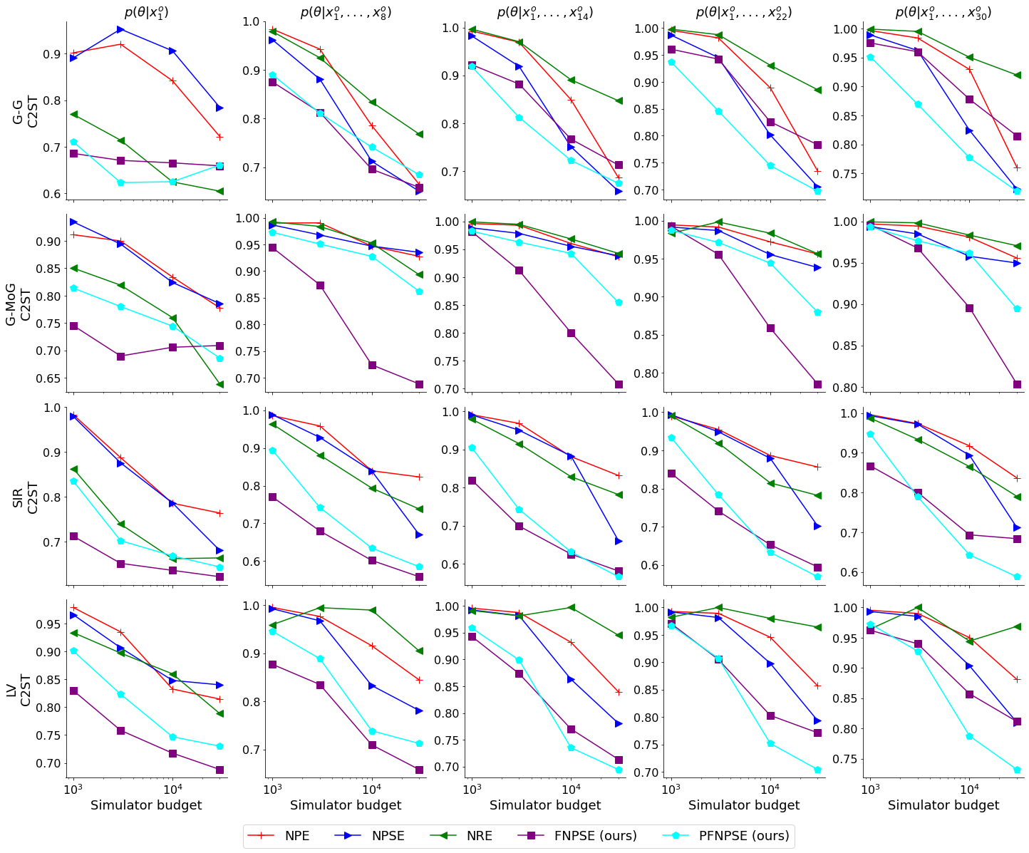
Figure 5: Classifier two-sample test scores (C2ST, lower is better) obtained by each method on different tasks. Plots show “C2ST” ($y$-axis) vs. “simulator budget used for training” ($x$-axis), and each line corresponds to a different method. Rows correspond to the different models considered (Gaussian/Gaussian, Gaussian/Mixture of Gaussians, SIR, Lotka–Volterra), and columns to the different number of conditioning observations available at inference time (1, 8, 14, 22, 30). We use $n_{\max}=30$ for NPE and NPSE and $m=6$ for PF-NPSE.

E.2 Performance of PF-NPSE for Different $m$

Figure 6 shows the results obtained using PF-NPSE for $m\in\{1,3,6,12,18,30\}$ to estimate the posterior distributions obtained by conditioning on a different number of observations in $\{1,8,14,22,30\}$. As pointed out in the main text, values of $m$ between $3$ and $6$ often lead to the best results.

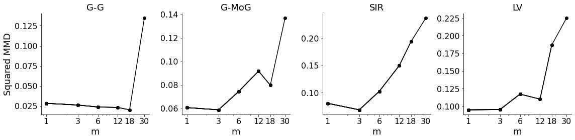
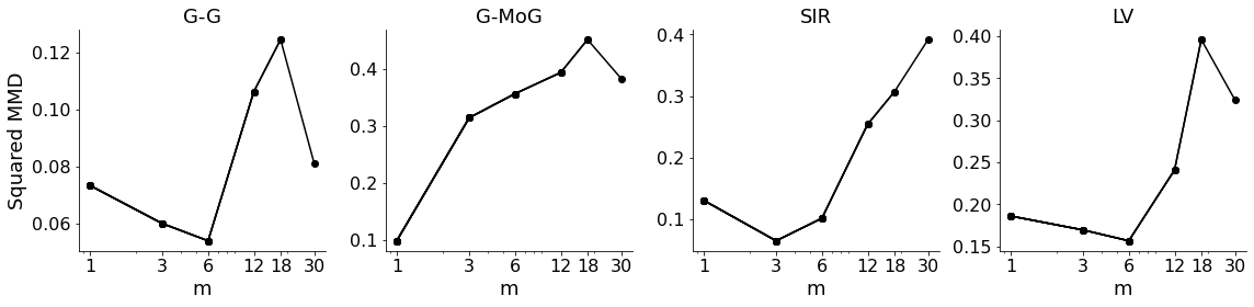
Figure 6: Plots show squared MMD (lower is better). Each column corresponds to a task (G-G, G-MoG, SIR, LV), and each row corresponds to approximating distributions obtained by conditioning on a different number of observations. From top to bottom, the number of conditioning observations we use is $1$, $8$, $14$, $22$, and $30$.

E.3 Conservative and Non-conservative Parameterization for the Score Network

Figure 7 compares the results obtained by score-modeling methods (NPSE, F-NPSE, and PF-NPSE) using different parameterizations for the score network. We consider the unconstrained parameterization typically used, where the score network outputs a vector of the same dimension as $\theta$, as well as a conservative parameterization, where the network outputs a scalar, and the score is obtained by computing its gradient. The figure shows that the choice of parameterization does not tend to have a substantial effect on performance.

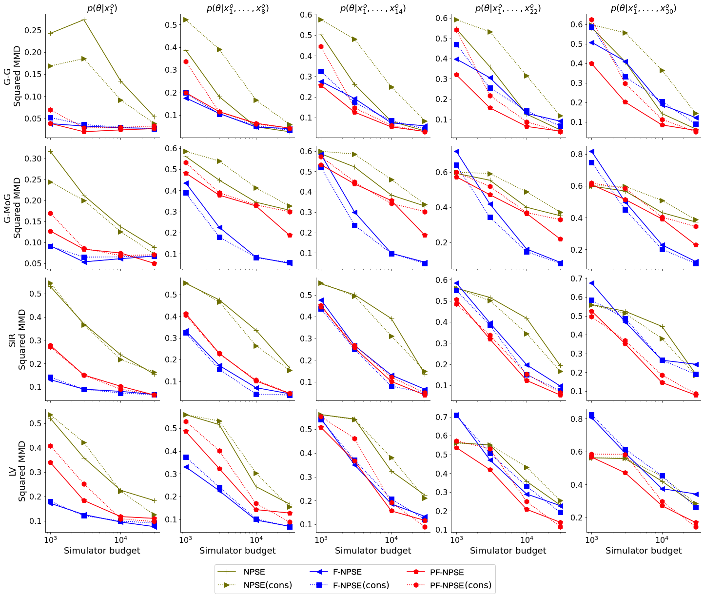
Figure 7: Squared MMD (lower is better) achieved by different methods on different tasks. Each row corresponds to a different model considered (Gaussian-Gaussian, Gaussian-Mixture of Gaussians, SIR, Lotka–Volterra), and each column to a different number of conditioning observations available at inference time (1, 8, 14, 22, 30). The (cons) identifier corresponds to methods using the conservative parameterization for the score network.

E.4 Langevin Sampler Parameters

Figure 8 shows the results obtained using PF-NPSE ($m=6$) with different parameters for the annealed Langevin sampler (Algorithm 1), and using the sampling method presented in Algorithm 2 (Appendix D), identified with comp in the figure’s legend. The method’s performance is robust to different parameters choices, as long as enough Langevin steps are taken at each noise level. We observe that 5 steps are often enough. Additionally, the results show that the sampling algorithm described in Appendix D (which does not rely on annealed Langevin dynamics) performs slightly worse than the Langevin sampler.

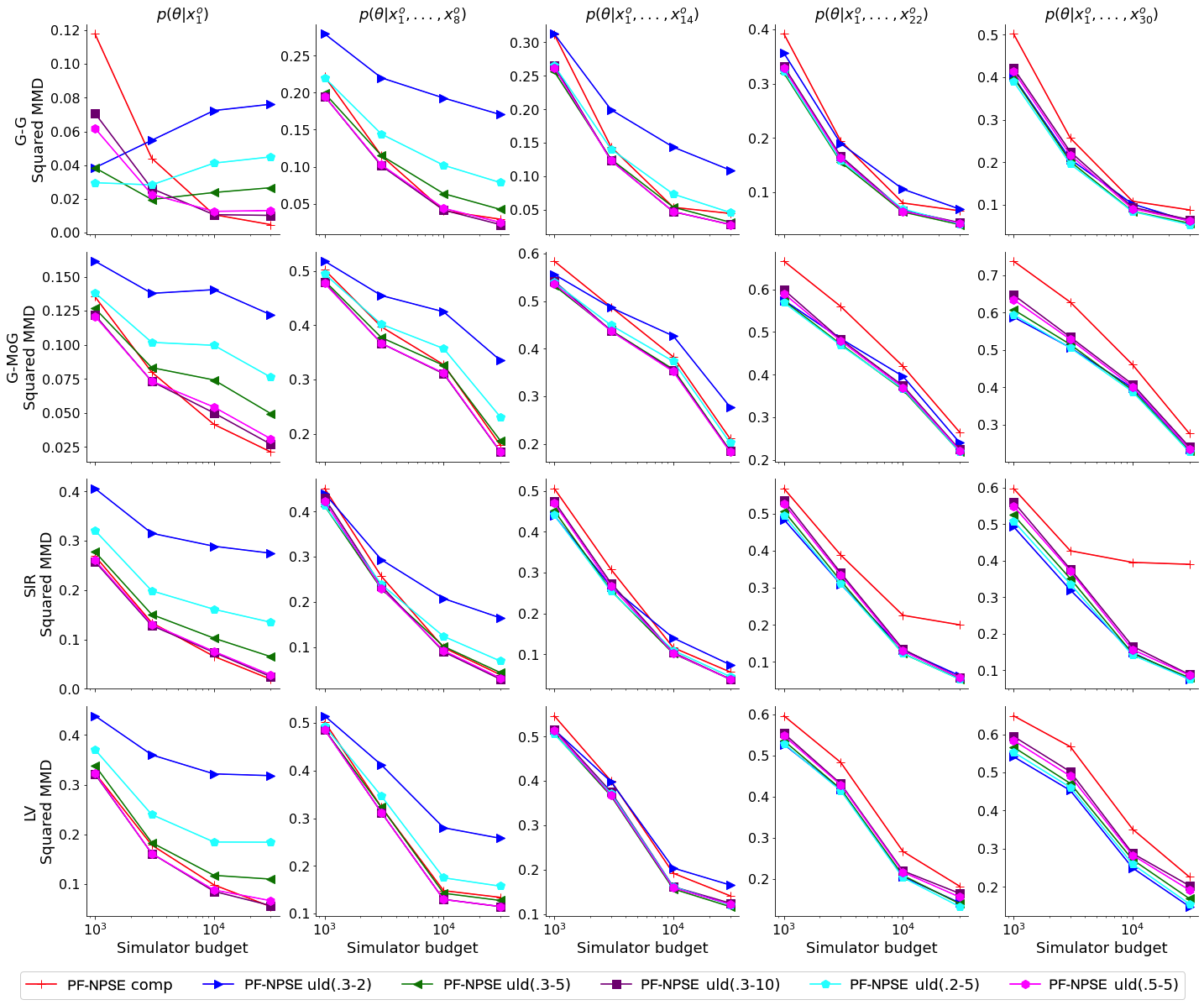
Figure 8: Squared MMD (lower is better) achieved by PF-NPSE ($m=6$) for different samplers. comp indicates sampling using Algorithm 2 (presented in Appendix D). uld(a-L) indicates sampling using annealed Langevin dynamics (Algorithm 1) with L steps per noise level and step-sizes $\delta_{t}=a\frac{1-\alpha_{t}}{\sqrt{\alpha_{t}}}$, where $\alpha_{1}=\gamma_{1}$ and $\alpha_{t}=\frac{\gamma_{t}}{\gamma_{t-1}}$ for $t=2,\ldots,T-1$.

References

- Ba et al. (2016) Ba, J. L., Kiros, J. R., and Hinton, G. E. Layer normalization. arXiv preprint arXiv:1607.06450, 2016.
- Batzolis et al. (2021) Batzolis, G., Stanczuk, J., Schönlieb, C.-B., and Etmann, C. Conditional image generation with score-based diffusion models. arXiv preprint arXiv:2111.13606, 2021.
- Beaumont (2019) Beaumont, M. A. Approximate Bayesian computation. Annual review of statistics and its application, 6:379–403, 2019.
- Blum & François (2010) Blum, M. G. B. and François, O. Non-linear regression models for approximate Bayesian computation. Statistics and Computing, 20(1):63–73, 2010.
- Chan et al. (2018) Chan, J., Perrone, V., Spence, J., Jenkins, P., Mathieson, S., and Song, Y. A likelihood-free inference framework for population genetic data using exchangeable neural networks. Advances in Neural Information Processing Systems, 31, 2018.
- Choi et al. (2022) Choi, K., Meng, C., Song, Y., and Ermon, S. Density ratio estimation via infinitesimal classification. In International Conference on Artificial Intelligence and Statistics, pp. 2552–2573. PMLR, 2022.
- Cranmer et al. (2015) Cranmer, K., Pavez, J., and Louppe, G. Approximating likelihood ratios with calibrated discriminative classifiers. arXiv preprint arXiv:1506.02169, 2015.
- Cranmer et al. (2017) Cranmer, K., Heinrich, L., Head, T., and Louppe, G. Active sciencing with reusable workflows. https://https://github.com/cranmer/active_sciencing, 2017.
- Cranmer et al. (2020) Cranmer, K., Brehmer, J., and Louppe, G. The frontier of simulation-based inference. Proceedings of the National Academy of Sciences, 117(48):30055–30062, 2020.
- De Bortoli et al. (2021) De Bortoli, V., Thornton, J., Heng, J., and Doucet, A. Diffusion Schrödinger bridge with applications to score-based generative modeling. Advances in Neural Information Processing Systems, 34:17695–17709, 2021.
- Del Moral et al. (2012) Del Moral, P., Doucet, A., and Jasra, A. An adaptive sequential Monte Carlo method for approximate Bayesian computation. Statistics and computing, 22(5):1009–1020, 2012.
- Dhariwal & Nichol (2021) Dhariwal, P. and Nichol, A. Diffusion models beat GANs on image synthesis. Advances in Neural Information Processing Systems, 34:8780–8794, 2021.
- Dinh et al. (2016) Dinh, L., Sohl-Dickstein, J., and Bengio, S. Density estimation using Real NVP. arXiv preprint arXiv:1605.08803, 2016.
- Du et al. (2023) Du, Y., Durkan, C., Strudel, R., Tenenbaum, J. B., Dieleman, S., Fergus, R., Sohl-Dickstein, J., Doucet, A., and Grathwohl, W. Reduce, reuse, recycle: Compositional generation with energy-based diffusion models and mcmc. arXiv preprint arXiv:2302.11552, 2023.
- Durkan et al. (2018) Durkan, C., Papamakarios, G., and Murray, I. Sequential neural methods for likelihood-free inference. Bayesian Deep Learning Workshop at Neural Information Processing Systems, 2018.
- Friedman (2003) Friedman, J. H. On multivariate goodness–of–fit and two–sample testing. Statistical Problems in Particle Physics, Astrophysics, and Cosmology, 1:311, 2003.
- Glöckler et al. (2022) Glöckler, M., Deistler, M., and Macke, J. H. Variational methods for simulation-based inference. arXiv preprint arXiv:2203.04176, 2022.
- Greenberg et al. (2019) Greenberg, D., Nonnenmacher, M., and Macke, J. Automatic posterior transformation for likelihood-free inference. In International Conference on Machine Learning, pp. 2404–2414. PMLR, 2019.
- Gretton et al. (2012) Gretton, A., Borgwardt, K. M., Rasch, M. J., Schölkopf, B., and Smola, A. A kernel two-sample test. The Journal of Machine Learning Research, 13(1):723–773, 2012.
- Harko et al. (2014) Harko, T., Lobo, F. S., and Mak, M. Exact analytical solutions of the Susceptible-Infected-Recovered (SIR) epidemic model and of the SIR model with equal death and birth rates. Applied Mathematics and Computation, 236:184–194, 2014.
- He et al. (2016) He, K., Zhang, X., Ren, S., and Sun, J. Deep residual learning for image recognition. In Proceedings of the IEEE conference on computer vision and pattern recognition, pp. 770–778, 2016.
- Hermans et al. (2020a) Hermans, J., Begy, V., and Louppe, G. Likelihood-free MCMC with amortized approximate ratio estimators. In International Conference on Machine Learning, pp. 4239–4248. PMLR, 2020a.
- Hermans et al. (2020b) Hermans, J., Begy, V., and Louppe, G. Likelihood-free MCMC with amortized approximate ratio estimators. In Proceedings of the 37th International Conference on Machine Learning, 2020b.
- Ho & Salimans (2022) Ho, J. and Salimans, T. Classifier-free diffusion guidance. arXiv preprint arXiv:2207.12598, 2022.
- Ho et al. (2020) Ho, J., Jain, A., and Abbeel, P. Denoising diffusion probabilistic models. Advances in Neural Information Processing Systems, 33:6840–6851, 2020.
- Hoffman et al. (2014) Hoffman, M. D., Gelman, A., et al. The No-U-Turn Sampler: adaptively setting path lengths in Hamiltonian Monte Carlo. J. Mach. Learn. Res., 15(1):1593–1623, 2014.
- Hyvärinen & Dayan (2005) Hyvärinen, A. and Dayan, P. Estimation of non-normalized statistical models by score matching. Journal of Machine Learning Research, 6(4), 2005.
- Kingma & Ba (2014) Kingma, D. P. and Ba, J. Adam: A method for stochastic optimization. arXiv preprint arXiv:1412.6980, 2014.
- Li et al. (2022) Li, H., Yang, Y., Chang, M., Chen, S., Feng, H., Xu, Z., Li, Q., and Chen, Y. Srdiff: Single image super-resolution with diffusion probabilistic models. Neurocomputing, 479:47–59, 2022.
- Liu et al. (2022) Liu, N., Li, S., Du, Y., Torralba, A., and Tenenbaum, J. B. Compositional visual generation with composable diffusion models. In Computer Vision–ECCV 2022: 17th European Conference, Tel Aviv, Israel, October 23–27, 2022, Proceedings, Part XVII, pp. 423–439. Springer, 2022.
- Louppe et al. (2017) Louppe, G., Hermans, J., and Cranmer, K. Adversarial variational optimization of non-differentiable simulators. arXiv preprint arXiv:1707.07113, 2017.
- Lueckmann et al. (2017) Lueckmann, J.-M., Goncalves, P. J., Bassetto, G., Öcal, K., Nonnenmacher, M., and Macke, J. H. Flexible statistical inference for mechanistic models of neural dynamics. Advances in Neural Information Processing Systems, 30, 2017.
- Lueckmann et al. (2019) Lueckmann, J.-M., Bassetto, G., Karaletsos, T., and Macke, J. H. Likelihood-free inference with emulator networks. In Symposium on Advances in Approximate Bayesian Inference, pp. 32–53. PMLR, 2019.
- Lueckmann et al. (2021) Lueckmann, J.-M., Boelts, J., Greenberg, D., Goncalves, P., and Macke, J. Benchmarking simulation-based inference. In International Conference on Artificial Intelligence and Statistics, pp. 343–351. PMLR, 2021.
- Luo (2022) Luo, C. Understanding diffusion models: A unified perspective. arXiv preprint arXiv:2208.11970, 2022.
- Marjoram et al. (2003) Marjoram, P., Molitor, J., Plagnol, V., and Tavaré, S. Markov chain Monte Carlo without likelihoods. Proceedings of the National Academy of Sciences, 100(26):15324–15328, 2003.
- Neal (2011) Neal, R. M. MCMC using Hamiltonian dynamics. Handbook of Markov chain Monte Carlo, 2(11):2, 2011.
- Nichol et al. (2022) Nichol, A. Q., Dhariwal, P., Ramesh, A., Shyam, P., Mishkin, P., Mcgrew, B., Sutskever, I., and Chen, M. GLIDE: Towards photorealistic image generation and editing with text-guided diffusion models. In Proceedings of the 39th International Conference on Machine Learning, 2022.
- Papamakarios & Murray (2016) Papamakarios, G. and Murray, I. Fast -free inference of simulation models with Bayesian conditional density estimation. Advances in Neural Information Processing Systems, 29, 2016.
- Papamakarios et al. (2019) Papamakarios, G., Sterratt, D., and Murray, I. Sequential neural likelihood: Fast likelihood-free inference with autoregressive flows. In The 22nd International Conference on Artificial Intelligence and Statistics, pp. 837–848. PMLR, 2019.
- Pham et al. (2014) Pham, K. C., Nott, D. J., and Chaudhuri, S. A note on approximating ABC-MCMC using flexible classifiers. Stat, 3(1):218–227, 2014.
- Phan et al. (2019) Phan, D., Pradhan, N., and Jankowiak, M. Composable effects for flexible and accelerated probabilistic programming in NumPyro. arXiv preprint arXiv:1912.11554, 2019.
- Radev et al. (2020) Radev, S. T., Mertens, U. K., Voss, A., Ardizzone, L., and Köthe, U. BayesFlow: Learning complex stochastic models with invertible neural networks. IEEE transactions on neural networks and learning systems, 2020.
- Ramdas et al. (2015) Ramdas, A., Reddi, S. J., Póczos, B., Singh, A., and Wasserman, L. On the decreasing power of kernel and distance based nonparametric hypothesis tests in high dimensions. In Proceedings of the AAAI Conference on Artificial Intelligence, volume 29, 2015.
- Ramesh et al. (2022) Ramesh, A., Dhariwal, P., Nichol, A., Chu, C., and Chen, M. Hierarchical text-conditional image generation with CLIP latents. arXiv preprint arXiv:2204.06125, 2022.
- Rezende & Mohamed (2015) Rezende, D. and Mohamed, S. Variational inference with normalizing flows. In International Conference on Machine Learning, pp. 1530–1538. PMLR, 2015.
- Rhodes et al. (2020) Rhodes, B., Xu, K., and Gutmann, M. U. Telescoping density-ratio estimation. Advances in neural information processing systems, 33:4905–4916, 2020.
- Roberts & Tweedie (1996) Roberts, G. O. and Tweedie, R. L. Exponential convergence of Langevin distributions and their discrete approximations. Bernoulli, 2(4):341–363, 1996.
- Saharia et al. (2022a) Saharia, C., Chan, W., Saxena, S., Li, L., Whang, J., Denton, E., Ghasemipour, S. K. S., Ayan, B. K., Mahdavi, S. S., Lopes, R. G., et al. Photorealistic text-to-image diffusion models with deep language understanding. arXiv preprint arXiv:2205.11487, 2022a.
- Saharia et al. (2022b) Saharia, C., Ho, J., Chan, W., Salimans, T., Fleet, D. J., and Norouzi, M. Image super-resolution via iterative refinement. IEEE Transactions on Pattern Analysis and Machine Intelligence, 2022b.
- Salimans & Ho (2021) Salimans, T. and Ho, J. Should EBMs model the energy or the score? 2021.
- Sharrock et al. (2022) Sharrock, L., Simons, J., Liu, S., and Beaumont, M. Sequential neural score estimation: Likelihood-free inference with conditional score based diffusion models. arXiv preprint arXiv:2210.04872, 2022.
- Shi et al. (2022) Shi, Y., De Bortoli, V., Deligiannidis, G., and Doucet, A. Conditional simulation using diffusion Schrödinger bridges. arXiv preprint arXiv:2202.13460, 2022.
- Sisson et al. (2007) Sisson, S. A., Fan, Y., and Tanaka, M. M. Sequential Monte Carlo without likelihoods. Proceedings of the National Academy of Sciences, 104(6):1760–1765, 2007.
- Sisson et al. (2018) Sisson, S. A., Fan, Y., and Beaumont, M. Handbook of approximate Bayesian computation. CRC Press, 2018.
- Sohl-Dickstein et al. (2015) Sohl-Dickstein, J., Weiss, E., Maheswaranathan, N., and Ganguli, S. Deep unsupervised learning using nonequilibrium thermodynamics. In International Conference on Machine Learning, pp. 2256–2265. PMLR, 2015.
- Song & Ermon (2019) Song, Y. and Ermon, S. Generative modeling by estimating gradients of the data distribution. Advances in Neural Information Processing Systems, 32, 2019.
- Song et al. (2020) Song, Y., Sohl-Dickstein, J., Kingma, D. P., Kumar, A., Ermon, S., and Poole, B. Score-based generative modeling through stochastic differential equations. arXiv preprint arXiv:2011.13456, 2020.
- Song et al. (2021) Song, Y., Durkan, C., Murray, I., and Ermon, S. Maximum likelihood training of score-based diffusion models. Advances in Neural Information Processing Systems, 34:1415–1428, 2021.
- Tabak & Turner (2013) Tabak, E. G. and Turner, C. V. A family of nonparametric density estimation algorithms. Communications on Pure and Applied Mathematics, 66(2):145–164, 2013.
- Tashiro et al. (2021) Tashiro, Y., Song, J., Song, Y., and Ermon, S. CSDI: Conditional score-based diffusion models for probabilistic time series imputation. Advances in Neural Information Processing Systems, 34:24804–24816, 2021.
- Vaswani et al. (2017) Vaswani, A., Shazeer, N., Parmar, N., Uszkoreit, J., Jones, L., Gomez, A. N., Kaiser, Ł., and Polosukhin, I. Attention is all you need. Advances in Neural Information Processing Systems, 30, 2017.
- Vincent (2011) Vincent, P. A connection between score matching and denoising autoencoders. Neural computation, 23(7):1661–1674, 2011.
- Welling & Teh (2011) Welling, M. and Teh, Y. W. Bayesian learning via stochastic gradient Langevin dynamics. In Proceedings of the 28th International Conference on Machine Learning, pp. 681–688. Citeseer, 2011.
- Winkler et al. (2019) Winkler, C., Worrall, D., Hoogeboom, E., and Welling, M. Learning likelihoods with conditional normalizing flows. arXiv preprint arXiv:1912.00042, 2019.
- Wiqvist et al. (2021) Wiqvist, S., Frellsen, J., and Picchini, U. Sequential neural posterior and likelihood approximation. arXiv preprint arXiv:2102.06522, 2021.
- Wood (2010) Wood, S. N. Statistical inference for noisy nonlinear ecological dynamic systems. Nature, 466(7310):1102–1104, 2010.
- Zaheer et al. (2017) Zaheer, M., Kottur, S., Ravanbakhsh, S., Poczos, B., Salakhutdinov, R. R., and Smola, A. J. Deep sets. Advances in neural information processing systems, 30, 2017.