DMAP: a Distributed Morphological Attention Policy for Learning to Locomote with a Changing Body

Abstract

Biological and artificial agents need to deal with constant changes in the real world. We study this problem in four classical continuous control environments, augmented with morphological perturbations. Learning to locomote when the length and the thickness of different body parts vary is challenging, as the control policy is required to adapt to the morphology to successfully balance and advance the agent. We show that a control policy based on the proprioceptive state performs poorly with highly variable body configurations, while an (oracle) agent with access to a learned encoding of the perturbation performs significantly better. We introduce DMAP, a biologically-inspired, attention-based policy network architecture. DMAP combines independent proprioceptive processing, a distributed policy with individual controllers for each joint, and an attention mechanism, to dynamically gate sensory information from different body parts to different controllers. Despite not having access to the (hidden) morphology information, DMAP can be trained end-to-end in all the considered environments, overall matching or surpassing the performance of an oracle agent. Thus DMAP, implementing principles from biological motor control, provides a strong inductive bias for learning challenging sensorimotor tasks. Overall, our work corroborates the power of these principles in challenging locomotion tasks.

1 Introduction

Animals and humans are highly adaptive to changes in the external environment and in their own body. For instance, animals can, after an early onset, locomote throughout their development despite dramatic changes in their body size and weight. Animals can also robustly deal with irregular surfaces, and load changes [1, 2, 3, 4, 5].

Here, we focus on the problem of learning to walk when the body is subject to morphological perturbations, i.e. changes in the length and thickness of body parts. Remarkably, animals can rapidly adapt to these kind of perturbations. For example, desert ants with elongated or shortened legs can immediately locomote, although misjudging the traveled distance [6]. To challenge artificial agents on such skills, we adapted four different locomotion environments (Ant, Half Cheetah, Walker, Hopper) from the OpenAI Gym [7], in which robots have to learn to walk as fast as possible. In our adaptive setting, the agent’s body parameters are sampled from a morphological perturbation space at the beginning of each episode and we sought to find reinforcement learning policies that could deal with these varying bodies.

We hypothesize that principles of the sensorimotor system provide a strong inductive bias to robustly learn such a policy. Specifically, we built on three well-known principles:

Independent low-level processing. Somatosensory inputs are first processed locally (e.g., by temporal filtering) before they are integrated across body parts and represented in an topographically ordered fashion [8, 9, 10].

Gated connectivity. Sensory information is dynamically gated in a task dependent manner [11, 12], and integrated with action and value signals in the brain [13, 10, 14].

Distributed control. Different body parts are controlled in a distributed fashion [9, 10, 5].

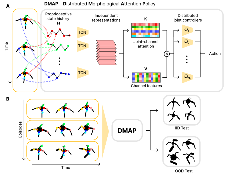
Figure 1: A. Overview of the architecture of DMAP. Each component of the state history is processed independently by a temporal convolutional network (with shared weights). The extracted features are transformed into the value encoding matrix and the attention weights of each joint sensor and action component. The product of these matrices results in a joint-specific morphology encoding, which is the convex combination of the value encoding vectors, weighted by their attention score. Independent fully-connected networks control a single joint, based on the current proprioceptive state and the morphology encoding B. DMAP is trained for several episodes with randomly sampled perturbed bodies within the training distribution. At test time, the zero-shot performance of the model is assessed on a fixed set of body configurations, sampled either from within (IID) or outside (OOD) of the training distribution.

Based on these principles, we propose the Distributed Morphological Attention Policy (DMAP) architecture (Figure 1). We show that DMAP can robustly learn to locomote with changing bodies without access to the morphological parameters. To assess the performance of DMAP, we compare it to several alternative agents: Simple, Oracle and rapid motor adaptation (RMA) [15]. Experiments reveal that an agent with access only to the proprioceptive state, consisting of its joint angles and velocities (Simple), fails to learn an effective locomotion strategy for a large variety of body configurations. In contrast, augmenting the observation with the current body parameters leads to a strong ceiling performance (Oracle). Remarkably, for all different environments, DMAP is as good as Oracle. We also compare DMAP to a powerful, recently proposed two-step training technique called rapid motor adaptation (RMA) [15]. This algorithm trains a temporal convolutional network to infer a context encoding from a short history of proprioceptive state, imitating the Oracle’s morphology encoder. While RMA can also reach Oracle performance, we show that end-to-end training of such a network does not succeed for more complicated environments (Ant and Walker). In contrast, DMAP’s policy can be trained end-to-end without access to the morphological parameters and reaches or surpasses Oracle performance for all four environments (Ant, Half Cheetah, Walker, Hopper).

Overall, our work suggests that independent low-level processing, distributed control and dynamic gating mechanisms provide a strong inductive bias for sensorimotor learning. Finally, we analyze the information gating mechanisms of DMAP. The strength of gated connections reveals morphology-specific patterns, such as bilateral and back-front symmetry. The low dimensional embedding of the gating mechanism exhibits rotational dynamics, robustly across different morphologies.

2 Related work

Benchmarks for zero-shot adaptation. The setup of the experiments described in this paper can be framed as a zero-shot adaptation problem, as the agents are evaluated starting from the first moment in which they interact with an unseen context [16]. While classic RL benchmarks, such as Arcade [17] and rllab [18], assess the ability of an agent to maximize the cumulative reward in the training environment, more recent ones introduce perturbations in the dynamics [19, 20], in the observation function [21, 22] or in the reward function [23] at test time. For a more complete list, we refer to the survey by Kirk et al. about generalization in Deep Reinforcement Learning [16]. Mann et al. showed that the performance of RL agents under morphological distributional shifts correlates with the ability of internal models to generalize [24]. We took their design of environments as an inspiration for the design of morphological changes in our work.

Context encoding and adaptation. Algorithms which enable learning in changing environments are important for the sim-to-real transfer problem, where domain randomization represents a successful strategy to bridge the reality gap [25, 26, 27]. A notable approach to solving the zero-shot transfer problem consists in encoding the context into a hidden state, e.g., by online system identification [28], or with a recurrent neural network (RNN) [18, 29]. However, while off-policy continuous control algorithms such as TD3 [30] and SAC [31] are the current state of the art among model-free RL algorithms, both in sample efficiency and final performance [32], training a recurrent neural network off-policy presents relevant technical challenges [33].

The problem of adaptation to an unseen environmental conditions is central in the Meta-RL literature [34]. Both model-based (ReBAL, GrBal [35], MOLe [36]), and model-free (PEARL [37]) algorithms prove capable to accelerate adaptation to unseen contexts. However, they require an adaptation phase in the test environment, which can last a few episodes [37] or some hours [35]. As the focus of our research is on the development of a network architecture to enable robust locomotion in a zero-shot manner, we chose to compare it to RMA, a powerful system identification approach; Kumar et al. showed that a context encoding can be successfully inferred from a short sequence of past states and actions, and this context encoding can guide a robust policy [15].

Distributed control. An agent can learn to generalize to multiple body shapes by using modular policies to control each joint independently, e.g., by treating each joint [38] or groups of joints [39] as a node of the graph. For example, Nervenet [40] achieves state-of-the-art performance on standard RL benchmarks by leveraging different policies for each joint type. However, it cannot generalize to different designs in a zero-shot manner (without fine-tuning). On the other hand, Shared Modular Policies (SMP) [41] employs the same policy for each joint, enabling an agent to deal with variable observation and action space sizes. Further solutions to handle bodies with variable connectivity graphs include transformer-based solutions, such as Amorpheus [42] and the recently proposed AnyMorph [43]. While these works study the problem of controlling bodies with a variable number of segments and connectivity graph, we focus on perturbations which affect morphological parameters, but without changing the body structure.

Hierarchical RL A common approach to solve complex RL tasks is to decompose them in a hierarchy of subproblems [44]. Walking with different body shapes could be interpreted as the union of a long-horizon task (locomotion) and a short-horizon one (body shape identification). Algorithms to tackle multi-horizon control problems by separating high-level behavior from motor primitives include Hierarchical Actor-Critic [45], HeLMS [46] and HiPPO [47].

3 A biology-inspired architecture to handle morphological perturbations

Adaptation to morphological perturbations requires an agent to rapidly identify which joints are affected and what compensatory torques are required. We propose a Distributed Morphological Attention Policy (DMAP) to address this problem (Figure 1). With DMAP, we seek to facilitate this process by promoting the formation of communication pathways from individual body parts to the specific joint controllers. The architecture is designed according to three principles of (biological) sensorimotor control (also mentioned in the introduction):

Independent low-level processing. Each proprioceptive channel is first processed independently, in order to obtain a channel-specific representation. This is inspired by the processing in the proprioceptive pathway [9, 10, 11].

Gated connectivity. An attention mechanism assigns the connection weight between the control policy of a joint and the features of each component of the proprioceptive state. This is inspired by dynamic gating mechanisms in the brain [11, 12, 13].

Distributed control. Independent networks control each of the agent’s joint, by outputting one single action scalar (corresponding to a joint’s torque). This is inspired by the architecture of the spinal cord and the motor homunculus [8, 2, 10].

We implemented those principles in the following way (Figure 1 and for more details Appendix A.1):

3.1 Independent processing and attention-based feature encoder

A feature encoder receives in input a history of $T$ proprioceptive states and actions $((\mathbf{s}^{(t-T)},\mathbf{a}^{(t-T)}),...,(\mathbf{s}^{(t-1)},\mathbf{a}^{(t-1)}))$, which we denote as $H^{(t)}\in\mathbb{R}^{(N_{S}+N_{A})\times T}$, $N_{S}$ and $N_{A}$ being the state and action space size, respectively. Each row $\mathbf{h}_{i}^{(t)}\in\mathbb{R}^{T}$ of $H^{(t)}$ is processed independently by the same Temporal Convolutional Network (TCN). A learned linear transformation maps each temporally-filtered input channel into the vectors $\mathbf{k}^{(t)}_{i}\in\mathbb{R}^{N_{A}}$, representing the attention of each joint towards that input channel $i$, and $\mathbf{v}^{(t)}_{i}\in\mathbb{R}^{N_{V}}$, a value encoding vector of size $N_{V}$ (a hyperparameter of the network). The vectors $\mathbf{k}^{(t)}_{i}$ and $\mathbf{v}^{(t)}_{i}$ from different channels are stacked to form the matrices $\tilde{K}^{(t)}\in\mathbb{R}^{(N_{S}+N_{A})\times N_{A}}$ and $V^{(t)}\in\mathbb{R}^{(N_{S}+N_{A})\times N_{V}}$. The matrix $K^{(t)}$ is obtained by applying a softmax operation to each column of $\tilde{K}^{(t)}$. The context encoding vectors for each joint controller are the rows $\mathbf{e}^{(t)T}$ of the matrix $E^{(t)}=K^{(t)T}V^{(t)}$, which are convex combinations of the features extracted from each sensory modality, weighted by their attention score (See diagram in Appendix A.1). This attention mechanism enables each controller to focus on the relevant morphological information carried by specific sensory channels, while ignoring the irrelevant ones. Furthermore, the attention matrix is conditioned to the recent transition history, making it adaptable both across episodes (and thus morphological states) and within a single episode.

3.2 Distributed joint controllers

Differently from standard policy networks, we adopt independent controllers $\Omega_{i}$, $i\in{{1,..,N_{A}}}$, for each joint, implemented as distinct fully-connected networks. Each network outputs the element $a_{i}^{(t)}$ of the action vector $\mathbf{a}^{(t)}$ based on the current state $\mathbf{s}^{(t)}$, the previous action $\mathbf{a}^{(t-1)}$ and the context encoding $\mathbf{e}^{(t)}_{i}$. Distributed action selection is a natural way to enable the emergence of sensorimotor pathways from the sensory data of different body parts to the controller of a joint. As one controller needs to predict one single action value, we show in our experiments that smaller fully-connected networks are sufficient to successfully solve the considered tasks, limiting the complexity overhead stemming from distributed control (See hyperparameters in Appendix A.2). Qualitatively, independent policy networks can more easily adapt their behavior when a morphological perturbation affects a localized area of the body, leaving the control policy of the other networks unaltered.

4 Morphological perturbation environments

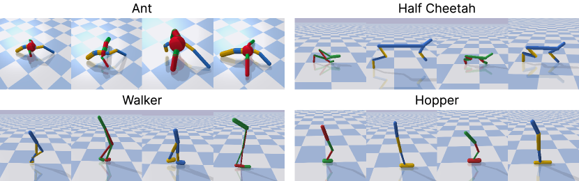
Figure 2: Example of perturbed body configurations for the four agents, sampled at the $\sigma=0.5$ perturbation level. The segments composing the body vary in thickness and length.

We consider four locomotion environments of the PyBullet physics simulator [48]: Hopper, Walker, Ant and Half-Cheetah, which are standard benchmarks for continuous control reinforcement learning algorithms [49, 32]. To test the ability of an agent to learn locomotion with a changing body, we introduce a set of morphological perturbations for each of them. The perturbations consist in modifying the size and the length of one or more body parts (Appendix A.3). Such perturbations strongly deteriorate the performance of an agent trained in the unperturbed environment [24]. The parameter $\sigma$ controls the size of the perturbation space $C_{\sigma}$, limiting the intensity of the perturbation between $-\sigma$ and $\sigma$. The perturbation is defined as the relative deviation of a morphological parameter from its original value. For example, a perturbation of 0.5 applied to a leg thickness will make it up to 1.5 times thicker. This construction results in widely varying body shapes for each of the four environments (Figure 2).

As in the unperturbed environments [32], the training is organized in episodes of at most 1000 time steps. At the beginning of each episode, bodily parameters are sampled uniformly at random in the space of admissible perturbations (and fixed throughout this episode). This setup defines a Contextual Markov Decision Process [16] $\mathcal{M}=\langle\mathcal{S},\mathcal{A},\mathcal{O},\mathcal{T},\mathcal{R},\gamma,C_{\sigma}\rangle$. $\mathcal{M}$ is determined by the state space $\mathcal{S}$, the observation function $\mathcal{O}$, the action space $\mathcal{A}$, the transition dynamics $\mathcal{T}$, the reward function $\mathcal{R}$, the discount factor $\gamma$ and the context $C_{\sigma}$. The observation only includes proprioceptive information, in the form of angular position and velocity of the joints, besides other non-visual variables (orientation of the body, contact forces with the floor; see Appendix A.3). The observation space $\mathcal{S}$ does not contain explicit information about the current context, as identical observations can come from bodies with different parameters. On the other hand, the context $c_{\sigma}\in C_{\sigma}$ influences the transition dynamics $p(\mathbf{s}_{t+1}|\,\mathbf{s}_{t},\mathbf{a}_{t},c_{\sigma})$, modifying the effect of an action depending on the body configuration. This condition of partial observability makes the locomotion problem considerably harder. However, confirming the intuition that contextual parameters influence the transition dynamics, we show that an agent can adapt by extracting information from the movement history.

Table 1: The five policy networks analyzed in the experiments. MLP: multi-layer perceptron. TCN: temporal-convolutional network. 2-step: imitation of the Oracle morphology encoder. P: proprioceptive state. M: morphology information. H: transition history.

	Simple	Oracle	RMA	TCN	DMAP
Encoder	-	MLP	TCN	TCN	Attention
Policy	MLP	MLP	MLP	MLP	Distributed MLP
Input	P	P + M	P + H	P + H	P + H
Training	End-to-end	End-to-end	2-step	End-to-end	End-to-end

5 Experiments

We trained all the agents with Soft Actor Critic (SAC) [31], using the open source library RLLib [50]. The experiments have been run on a local CPU cluster, for a total of approx. 100 000 cpu-hours. We used similar hyperparameters to Raffin et al. [32], which provide state-of-the-art results in the base versions of the four PyBullet environments considered in our work (Appendix A.3). We ran every experiment for 5 random seeds. We found that the training of the critic network benefits slightly from augmenting the input observation with the current morphological perturbation. Therefore, we included it for all policy architectures, except for the Simple agent. This addition does not pose any limitation to the deployment of the proposed algorithms, as the policy network alone is necessary at that stage.

The experiments involve five different policy networks (Simple, Oracle, RMA, TCN, DMAP), which differ in architecture, required input data and training procedure (Table 1). During training, the morphology parameters are randomly sampled from a perturbation space, defined by the parameter $\sigma$, at the beginning of each episode. An episode lasts 1000 time steps, unless an early termination condition is met (in case the agent falls). In this time, the agent has to learn to adapt to its unseen body configuration and run as fast as possible.

We evaluate the performance of a trained agent on its ability to adapt in a zero-shot manner to an unseen body morphology. To do so, we use a test set of 100 body configurations for each perturbation intensity, which were not part of the body configurations used during the training phase. The agent is tested on a single episode per test morphology, in which it only observes the proprioceptive states (without any information about the body state - except for the Oracle). During the testing phase, the agent does not observe the rewards it collects. We apply this testing protocol to the performance evaluation of all the trained policies and all the environments and perturbation levels. To evaluate the agent’s ability to adapt to an unseen morphology, we consider the reward it accumulates in the complete test episode (without changing the policy; zero-shot setting). We do so for all the body configurations in the test set. Table 2 and the tables in Appendix A.4 list the zero-shot performance of all the trained agents in different test environments. The rewards in bold are significantly higher according to a paired t-test (p-value < 0.001). We denote the tests as IID if the 100 body configurations were extracted from the morphological space used during the training ($\sigma_{train}\geq\sigma_{test}$), otherwise we denote them as OOD ($\sigma_{train}<\sigma_{test}$).

5.1 A morphology encoding boosts learning in strongly perturbed environments

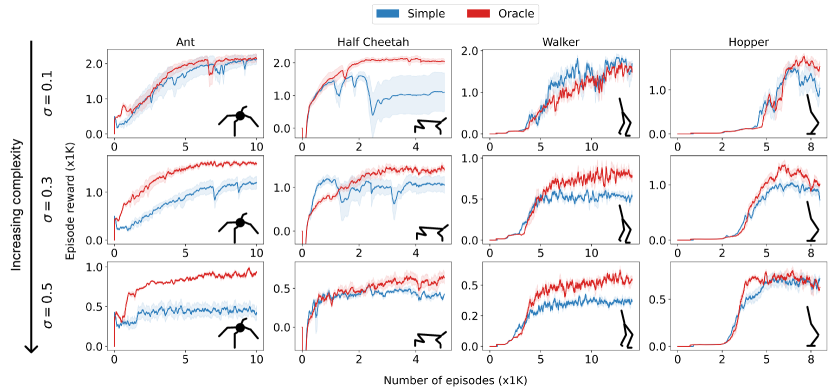
Figure 3: Learning curves of Simple and Oracle (mean ± SEM across 5 random seeds). While the Simple performs competitively in low perturbation environments ($\sigma=0.1$), Oracle learns better at higher perturbation levels.

To assess whether an agent can benefit from an encoding of its morphology when learning a locomotion policy, we compare the performance achieved when providing only the proprioceptive state (Simple) and when augmenting it with the perturbation parameters (Oracle). Specifically, this Oracle follows the architecture of Kumar et al. [15]. It extracts a morphology encoding from the raw perturbation vector and concatenates it to the observation vector, thus augmenting the input of the policy network and breaking the partial observability of the environment. We found that, while in mildly perturbed environments Simple performs competitively with Oracle, learning a control policy solely based on the proprioceptive state becomes difficult with increasing perturbation strength (Figure 3 and Appendix A.4). In all our experiments with $\sigma\in\{0.3,0.5\}$, learning a morphology representation improved performance (Table T4). This demonstrates, as expected, that learning an environment encoding is a viable option to deal with strongly perturbed environments.

5.2 The morphology encoding can be regressed from experience

The morphology parameters $c_{\sigma}\in C_{\sigma}$ influence the transition dynamics $p(\mathbf{s}_{t+1}|\,\mathbf{s}_{t},\mathbf{a}_{t},c_{\sigma})$ by changing the physical properties of the body. Therefore, they are implicitly represented in a sequence of transitions, from which they might be inferred. To test this possibility, we consider a recently proposed algorithm for adaptive locomotion called rapid motor adaptation (RMA) [15]. It leverages the latent representation of the body generated by a trained Oracle, which has access to the contextual information, to train a TCN network to regress the context encoding from a short history of $T$ proprioceptive states and actions $H^{(t)}=((\mathbf{s}^{(t-T)},\mathbf{a}^{(t-T)}),...,(\mathbf{s}^{(t-1)},\mathbf{a}^{(t-1)}))$ with $T=30$ transitions (see Appendix A.2 for hyperparameters).

Table 2: IID performance of RMA and Oracle, mean episode reward $\pm$ SEM.

Env	Ant		Half Cheetah		Walker		Hopper
Algo	RMA	Oracle	RMA	Oracle	RMA	Oracle	RMA	Oracle
$\sigma=0.1$	$2138\pm 16$	$2148\pm 16$	$2197\pm 16$	$2203\pm 17$	$1750\pm 28$	$1780\pm 26$	$1859\pm 19$	$1859\pm 18$
$\sigma=0.3$	$1700\pm 17$	$1723\pm 18$	$1402\pm 27$	$1\mathbf{469\pm 24}$	$836\pm 23$	$\mathbf{908\pm 23}$	$1267\pm 27$	$1296\pm 26$
$\sigma=0.5$	$966\pm 16$	$974\pm 18$	$595\pm 26$	$\mathbf{668\pm 24}$	$579\pm 17$	$\mathbf{625\pm 17}$	$730\pm 21$	$\mathbf{919\pm 18}$

RMA achieves similar average reward to the Oracle (Table 2). Thus, a sequence of 30 transitions of previous proprioceptive states and actions (approx. 0.5 s in our experiments) is sufficient to extract an embedding of the context that yields high reward. This demonstrates that RMA’s two-phase adaptation procedure is also viable for morphological perturbations.

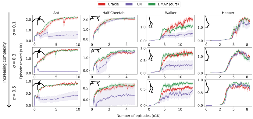
Figure 4: Learning curves of Oracle, DMAP and TCN, the network architecture used in RMA, but trained end-to-end (mean ± SEM across 5 random seeds). The performance gap between TCN and DMPAP is particularly clear for Ant and Walker, in which the training of TCN is characterized by high variance and overall low reward. Overall, DMAP, without access to the perturbation state, matches the learning performance of Oracle in most environments, with the exception of Walker $\sigma=0.1$, where Oracle is better, and Walker $\sigma=0.5$, where DMAP is better.

5.3 DMAP enables end-to-end training of a morphology encoding network

Our RMA experiments demonstrated that a temporal convolutional network can regress the morphology encoding from a sequence of proprioceptive states and actions representing 0.5 seconds of transition history. However, it is unclear whether RMA’s TCN encoder requires RMA’s two-step training through imitation to successfully extract a morphology encoding from a sequence of transitions. In fact, if such an encoding helps maximizing the reward, the TCN might successfully learn to extract the same representation by end-to-end reinforcement learning.

Remarkably, end-to-end training of a TCN encoder proves successful for the Hopper and the Half Cheetah. However, we encountered strong instability for the Ant and Walker across the random seeds (Figure 4). Surprisingly, in these two latter environments the addition of the TCN encoder is even harmful for the overall performance, as Simple achieves stronger results in the same environments (Appendix A.4). Further analysis reveals that for certain random seeds, the training process is disrupted before the agent can learn how to walk (Appendix A.4).

We hypothesize that this inability to learn is due to the difficulty of extracting a meaningful encoding to directly optimize the reward without a suitable inductive bias. For complex morphologies, the TCN encoder might even act as a confounder for the policy network. Indeed, replacing the TCN with DMAP leads to better stability during the training (Figure 4) and to a general performance improvement, particularly for the Ant and Walker (Appendix A.4). Differently from TCN, DMAP performs on par with Oracle in all the considered environments, with the exception of Walker with $\sigma=0.1$. Oracle and DMAP also perform similarly when tested OOD, with a slight advantage for DMAP (Figure 5 and Appendix A.4, A.5). Finally, we compared the adaptation speed of RMA and DMAP to unseen morphological perturbations. We found that the two algorithms perform motor adaptation equally fast (Appendix A.6). Thus, DMAP learns to robustly locomote in an end-to-end fashion, without access to the morphology parameters.

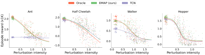
Figure 5: Reward obtained by Oracle, TCN and DMAP, trained in the $\sigma=0.3$ environments, on a wide range of perturbations (both IID and OOD). Each point represents the average reward across 5 random seeds for one body configuration, while the perturbation intensity is the eucledian norm of the perturbation vector. The curves are obtained by fitting a sigmoid function. Despite the larger perturbations falling outside of the training distribution, DMAP slightly outperforms Oracle, which receives the exact perturbation information. TCN performs worse for more challenging morphologies (Ant, Walker).

5.4 Ablation: The morphology encoding is key in statically unstable environments

To isolate the contribution of the morphology encoding on the performance of DMAP, we performed test-time ablation by evaluating the trained, distributed DMAP policy, while removing the morphology encoding. We found a performance drop for all the environments and perturbation levels (Table 3). This performance decay is especially severe in Hopper and Walker (approx. $50\%$), where the controller with ablated encoding fails to stabilize the agents, causing the early termination condition to be met sooner and thus yielding lower episode reward. This suggests that the attention mechanism is fundamental for the dynamic stability of these agents.

Table 3: IID performance of DMAP and non-encoding/ablated (ne) DMAP, mean episode reward $\pm$ SEM.

Env	Ant		Half Cheetah		Walker		Hopper
Algo	DMAP	DMAP-ne	DMAP	DMAP-ne	DMAP	DMAP-ne	DMAP	DMAP-ne
$\sigma=0.1$	$\mathbf{2240\pm 11}$	$1966\pm 18$	$\mathbf{2261\pm 11}$	$1493\pm 15$	$\mathbf{1229\pm 24}$	$337\pm 16$	$\mathbf{1842\pm 18}$	$984\pm 33$
$\sigma=0.3$	$\mathbf{1623\pm 19}$	$1542\pm 19$	$\mathbf{1577\pm 22}$	$1132\pm 29$	$\mathbf{893\pm 11}$	$470\pm 16$	$\mathbf{1316\pm 24}$	$748\pm 23$
$\sigma=0.5$	$\mathbf{960\pm 14}$	$881\pm 12$	$\mathbf{669\pm 23}$	$507\pm 29$	$\mathbf{743\pm 15}$	$341\pm 17$	$\mathbf{953\pm 15}$	$482\pm 20$

5.5 How does attention gate sensorimotor information?

We hypothesized that DMAP enables the agent to learn which components of the input are relevant for each joint’s controller. Next, we verify that such pathways emerge by analyzing the values of the attentional matrix $K^{(t)}$, both in the steady and dynamic condition.

The steady attentional matrix $K$ represents the strength of each input to output (i.e., sensorimotor) connection. We computed morphology-specific patterns by averaging elements across time and episodes (Figure 6). As in the spinal cord, the controllers typically attend to the sensory input of mechanically linked parts (e.g., foot controller to foot velocity, etc.). Yet, this topography is not universal: for instance in the hopper, all controllers focus on the leg angle and the foot velocity. Furthermore, the attention patterns seem to reflect the bilateral symmetry of the Ant and Walker and a front-back asymmetry due to the directionality of the locomotion task. However, the attention maps developed by DMAP vary for different seeds, indeed even gait patterns can vary across seeds. Furthermore, many state and action parameters are correlated during simple locomotion. This makes interpreting why specific connections emerge in the attention maps challenging. Despite this, across seeds, we often observe bilateral and back-front symmetry. In the future, we want to study this with more challenging locomotion tasks that decorrelate the states (e.g. non-flat terrains).

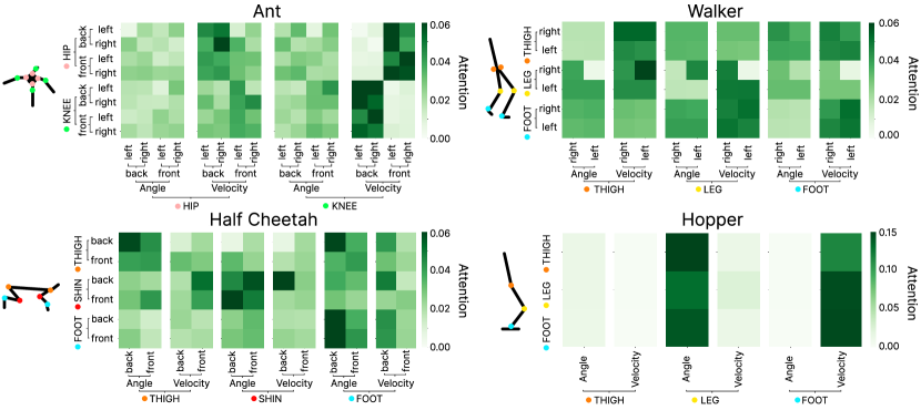
Figure 6: Attentional matrices $K$, averaged across time and IID test body perturbations, represented as a heatmap for each agent, trained with $\sigma=0.1$. We can observe several interpretable patterns, e.g., the bilateral symmetry in the Ant, as well as a front-back asymmetry (due to the fixed running direction). Also in the Ant, the hip controllers mainly look at the angular velocity of the front knees and of the back hips, while the ankle controllers do the opposite. In the Half Cheetah, too, the attention map develops a front-back asymmetry, with a preference for the input angular position, and each controller mainly attends to the state of the joint it controls.

To analyze the temporal evolution of attention, we projected the attentional matrix $K^{(t)}$ onto a 3-dimensional space learned with UMAP [51]. Depending on the phase of the gait, the attentional matrix $K^{(t)}$ strengthens or weakens specific sensorimotor pathways (Figure 7 A). The graphs reveal a rotational dynamics of the gain modulation typical of biological, legged locomotion [52, 53, 11]. Interestingly, in DMAP the attentional dynamics seem significantly less tangled than that of the proprioceptive and action input (Figure 7 B). We quantified this visual impression across different environments and found a robust effect (Appendix A.7). We speculate that this untangling mechanism might contribute to the robustness of the policy to morphological perturbations.

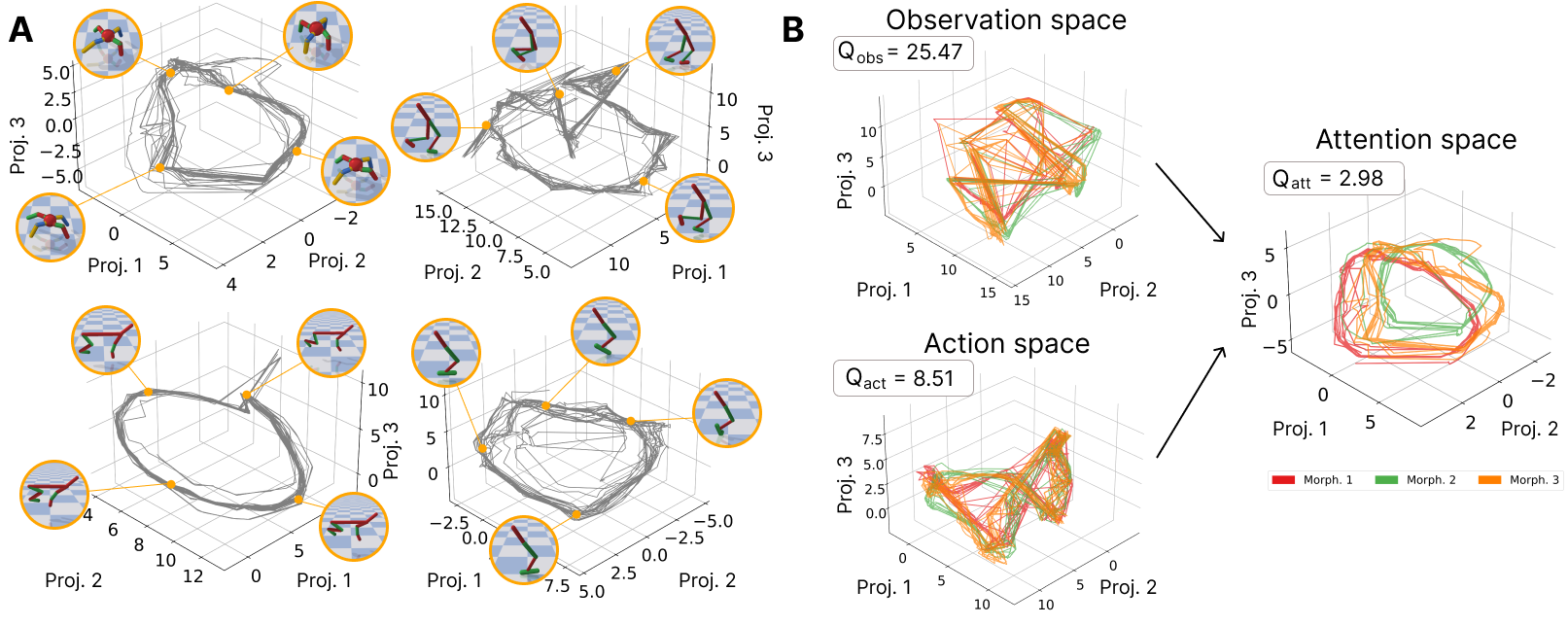
Figure 7: A. UMAP embedding of the attention matrix $K_{t}$ evolving during a single episode for each agent. The attentional dynamics of $K_{t}$ are cyclic, consistently with the periodic gait of the agents. Thus, the connectivity patterns between input channels and joint controllers change throughout the different phases of the gait. B. UMAP embeddings of the input observations $\mathcal{O}^{(t)}\in\mathbb{R}^{N_{S}\times T}$, input actions $\mathcal{A}^{(t)}\in\mathbb{R}^{N_{A}\times T}$ and attentional matrix $K_{t}$ for 3 different morphologies of the Ant. The change of body configuration causes a shift of the attentional dynamics in the low-dimensional space. The trajectories of the attention embedding seem less tangled than the corresponding input. We confirmed this impression by quantifying trajectories with a tangling metric $Q$ (averaged over time and morphologies). Larger values correspond to more tangled trajectories and the resulting $Q$ is shown in the plots. We refer to Appendix A.7 for more technical details.

6 Discussion

We proposed DMAP, a novel architecture that integrates computational principles of the sensorimotor system in reinforcement learning architectures. We find that DMAP enables the end-to-end training of a RL policies in environments with changing body parameters, without having access to the perturbation information. Thereby, DMAP matches or even surpasses the performance of an Oracle when tested in a zero-shot manner on unseen body configurations.

Interestingly, unlike DMAP, a TCN cannot be trained end-to-end to achieve robust locomotion for more complex morphologies (Section 5.3). Our work provides an example for biological principles providing excellent inductive biases for learning, consistent with the idea that innate, structured brain connectivity nurtures biological learning [54]. Furthermore, the attention mechanism of DMAP solves this challenging task by establishing gait-phase-dependent gain modulation, robust across morphologies. Notably, synaptic gains in the nervous system also change in a phase-dependent way [52, 53, 11].

Limitations and broader impact. One characteristic of our current architecture design is that each joint controller observes the full proprioceptive state. A future direction will be to limit the input to the local sensory data. Such design, separating low-latency sensorimotor connection (reflexes) and slower connections to distal body parts, would be closer to the locomotor system of the animals [2]. Furthermore, in our experiments, we have used an oracle critic to learn an estimate of the cumulative reward and guide the training of the policy. This gave slightly better results, however, a suitable inductive bias (like DMAP) or possibly inspired by the neural circuits responsible for reward prediction error, could remove this (training) limitation.

Our research aims to facilitate the training of control policies by transferring insights from neuroscience to artificial intelligence. Powerful reinforcement learning algorithms might find application in robotics, potentially enabling, in the long term, a large-scale deployment of autonomous agents. Automation comes with great opportunities, and ethical concerns [55].

Appendix A Appendix

A.1 DMAP detailed architecture

The Distributed Morphological Attention Policy (DMAP) consists of three main components: independent low-level proprioceptive processing, an attention-based morphology encoder and a distributed joint controller (Figure F1).

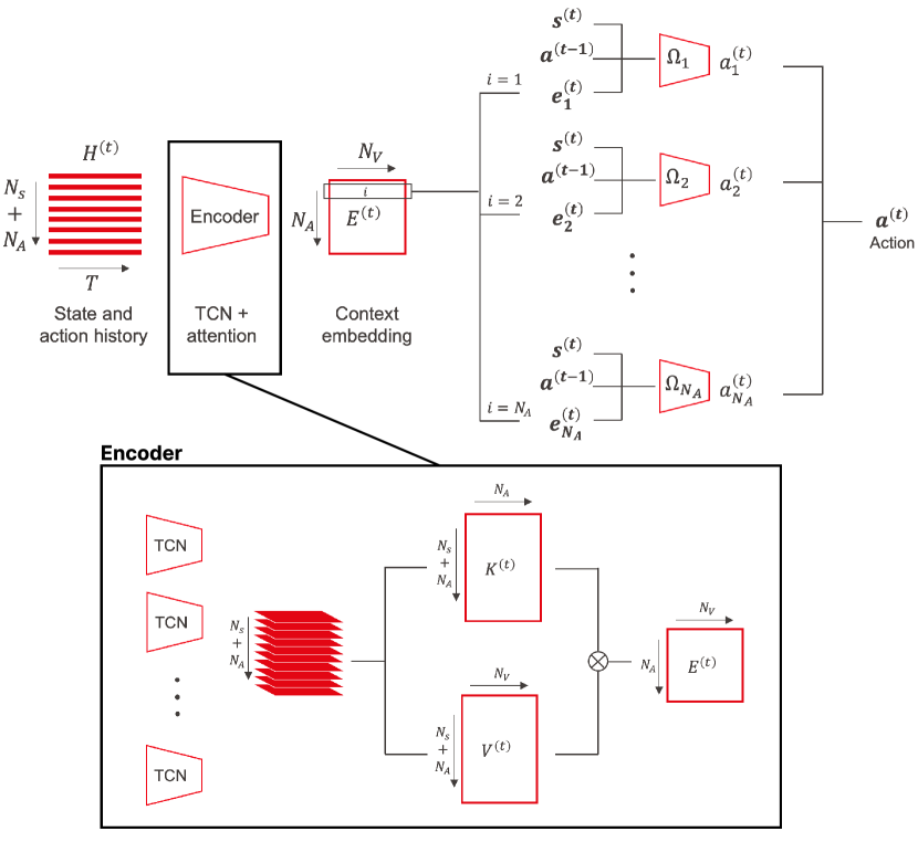
Figure F1: Detailed architecture of DMAP. After applying convolutions to the each input channel along the temporal dimension, the encoder module extracts: a key matrix $K^{(t)}$, whose elements represent the attention score of an action component towards an input channel; a value matrix $V^{(t)}$, whose rows encode the information from each input channel of the transition history. A softmax operation is applied along the columns of the $K^{(t)}$ matrix, so that the total attention of one action component sums to 1. The action component-specific encoding vectors $\mathbf{e}^{(t)}$ are obtained by matrix multiplication: $K^{(t)T}V^{(t)}$. The learned context embedding is then concatenated with the previous action $\mathbf{a}^{(t-1)}$ and the current proprioceptive observation $\mathbf{s}^{(t)}$. Together, those triples are the inputs to $N_{A}$ fully-connected networks, one for each action component. They output the torque applied to one joint of the agent.

A.2 Hyperparameters

Table T1 lists the hyperparameters of SAC used for our experiments. They are the same for all network architectures, without specific fine tuning. We also list the parameters of the neural networks of the different agents.

Table T1: Parameters of SAC for each of the 4 environments

Environment		Ant	Half Cheetah	Walker	Hopper
Algorithms	Parameters
All	Action normalization	Yes	Yes	Yes	Yes
	Num TD steps	1	1	1	1
	Buffer size	1 000 000	300 000	300 000	300 000
	Prioritized experience replay	No	Yes	Yes	Yes
	Actor learning rate	0.0003	0.0003	0.0003	0.0003
	Critic learning rate	0.0003	0.0003	0.0003	0.0003
	Entropy learning rate	0.0003	0.0003	0.0003	0.0003
	Discount factor $\gamma$	0.995	0.995	0.995	0.995
	Minibatch size	256	256	256	256
Simple	Policy hiddens	[256, 256]	[256, 256]	[256, 256]	[256, 256]
	Q hiddens	[256, 256]	[256, 256]	[256, 256]	[256, 256]
	Activation	ReLU	ReLU	ReLU	ReLU
Oracle	Policy encoder hiddens	[256, 128]	[256, 128]	[256, 128]	[256, 128]
	Encoding size	4	4	4	4
	Policy hiddens	[128, 128]	[128, 128]	[128, 128]	[128, 128]
	Q encoder hiddens	[256, 128]	[256, 128]	[256, 128]	[256, 128]
	Q hiddens	[128, 128]	[128, 128]	[128, 128]	[128, 128]
	Activation	ReLU	ReLU	ReLU	ReLU
RMA/TCN	Num TCN layers	3	3	3	3
	Num filters per layer	[32, 32, 32]	[32, 32, 32]	[32, 32, 32]	[32, 32, 32]
	Kernel size per layer	[5, 3, 3]	[5, 3, 3]	[5, 3, 3]	[5, 3, 3]
	Stride per layer	[4, 1, 1]	[4, 1, 1]	[4, 1, 1]	[4, 1, 1]
	Policy encoder hiddens	[128, 32]	[128, 32]	[128, 32]	[128, 32]
	Encoding size	4	4	4	4
	Policy hiddens	[128, 128]	[128, 128]	[128, 128]	[128, 128]
	Q encoder hiddens	[256, 128]	[256, 128]	[256, 128]	[256, 128]
	Q hiddens	[128, 128]	[128, 128]	[128, 128]	[128, 128]
	Activation	ReLU	ReLU	ReLU	ReLU
	History size T	30	30	30	30
DMAP	Num TCN layers	3	3	3	3
	Num filters per layer	[32, 32, 32]	[32, 32, 32]	[32, 32, 32]	[32, 32, 32]
	Kernel size per layer	[5, 3, 3]	[5, 3, 3]	[5, 3, 3]	[5, 3, 3]
	Stride per layer	[4, 1, 1]	[4, 1, 1]	[4, 1, 1]	[4, 1, 1]
	Policy encoder hiddens	[128, 32]	[128, 32]	[128, 32]	[128, 32]
	Encoding size	4	4	4	4
	Policy hiddens	[32, 32]	[32, 32]	[32, 32]	[32, 32]
	Num policy networks	8	6	6	3
	Q encoder hiddens	[256, 128]	[256, 128]	[256, 128]	[256, 128]
	Q hiddens	[128, 128]	[128, 128]	[128, 128]	[128, 128]
	Activation	ReLU	ReLU	ReLU	ReLU
	History size T	30	30	30	30

A.3 Perturbed environments specifications

The state and action components of the four perturbed environments (Ant, Half Cheetah, Walker, Hopper) are the same as the ones of the environment they are derived from. They are listed in Table T2, ordered as they appear in the state and action vectors. The body parameters are sampled from a uniform distribution at the beginning of each episode. The body segments are perturbed in small subgroups, e.g., the two segments forming a limb of Ant, in which the perturbation is consistent. The parameters defining the perturbation space are detailed in Table T3.

During our experiments, we experienced an unusual behavior in the Half Cheetah environment for particularly light limbs (i.e., ones with small thickness). In this case, the Cheetah could move the legs at very high speed. In this case, PyBullet allowed an unnatural locomotion, in which the agent could advance without touching the ground, seemingly ignoring gravity. For this reason, we set a lower bound to the perturbation on the length and the thickness of the limbs, corresponding to $-0.3$ (only for the Half Cheetah with $\sigma=0.5$). This clipping removed the unusual behavior of the simulator.

Table T2: State and action components of each environment. $\alpha$ is the angle between the target direction and the current running direction. $v_{i}$, $i\in{{x,y,z}}$ are the components of the linear velocity vector.

Environment	Ant	Half Cheetah	Walker	Hopper
Components
State	Elevation	Elevation	Elevation	Elevation
	$sin(\alpha)$	$sin(\alpha)$	$sin(\alpha)$	$sin(\alpha)$
	$cos(\alpha)$	$cos(\alpha)$	$cos(\alpha)$	$cos(\alpha)$
	$v_{x}$	$v_{x}$	$v_{x}$	$v_{x}$
	$v_{y}$	$v_{y}$	$v_{y}$	$v_{y}$
	$v_{z}$	$v_{z}$	$v_{z}$	$v_{z}$
	roll	roll	roll	roll
	pitch	pitch	pitch	pitch
	Back left hip angle	Back thigh angle	Right thigh angle	Thigh angle
	Back left hip velocity	Back thigh velocity	Right thigh velocity	Thigh velocity
	Back left knee angle	Back shin angle	Right leg angle	Leg angle
	Back left knee velocity	Back shin velocity	Right leg velocity	Leg velocity
	Front left hip angle	Back foot angle	Right foot angle	Foot angle
	Front left hip velocity	Back foot velocity	Right foot velocity	Foot velocity
	Front left knee angle	Front thigh angle	Left thigh angle	Foot contact
	Front left knee velocity	Front thigh velocity	Left thigh velocity
	Back right hip angle	Front foot angle	Left leg angle
	Back right hip velocity	Front foot velocity	Left leg velocity
	Back right knee angle	Front foot contact	Left foot angle
	Back right knee velocity	Front shin contact	Left foot velocity
	Front right hip angle	Front thigh contact	Right foot contact
	Front right hip velocity	Back foot contact	Left foot contact
	Front right knee angle	Back shin contact
	Front right knee velocity	Back thigh contact
	Back left foot contact
	Front left foot contact
	Back right foot contact
	Front right foot contact
Action	Back left hip torque	Front foot torque	Right thigh torque	Thigh torque
	Back left knee torque	Front shin torque	Right leg torque	Leg torque
	Front left hip torque	Front thigh torque	Right foot torque	Foot torque
	Front left knee torque	Back foot torque	Left thigh torque
	Back right hip torque	Back shin torque	Left leg torque
	Back right knee torque	Back thigh torque	Left foot torque
	Front right hip torque
	Front right knee torque

Table T3: Perturbation parameters of each environment.

Environment	Ant	Half Cheetah	Walker	Hopper
Perturbation type
Thickness	Torso	Head	Torso	Torso
	Front left limb	Torso	Limbs	Limb
	Front right limb	Back limb	Feet	Foot
	Back left limb	Front limb
	Back right limb
Length	Front left limb	Torso	Limbs	Limb
	Front right limb	Back limb	Feet	Foot
	Back left limb	Front limb
	Back right limb
Total	9	7	5	5

A.4 Performance summary

Tables T4 and T5 compare the IID performance of Simple-Oracle and of TCN and DMAP. The numbers in bold denote a significant statistical difference between the two methods (p-value $<0.001$, paired t-test).

We also list the IID (Table T6) and OOD (Tables T7, T8 and T9) test results of all the agents trained for this work. Some negative values should not surprise the reader, as some agents, when tested way outside of the training distribution, fail to walk, collecting more penalties (e.g., due to undesired contact force or excessive energy expenditure) than positive reward.

Table T4: IID performance of Simple and Oracle, mean episode reward $\pm$ SEM across 5 different random seeds, on 100 body configurations not encountered during the training.

Env	Ant		Half Cheetah		Walker		Hopper
Algo	Simple	Oracle	Simple	Oracle	Simple	Oracle	Simple	Oracle
$\sigma=0.1$	$2164\pm 17$	$2148\pm 16$	$1633\pm 25$	$\mathbf{2203\pm 17}$	$\mathbf{1909\pm 17}$	$1780\pm 26$	$1807\pm 25$	$1859\pm 18$
$\sigma=0.3$	$1270\pm 20$	$\mathbf{1723\pm 18}$	$1412\pm 22$	$\mathbf{1469\pm 24}$	$691\pm 17$	$\mathbf{908\pm 23}$	$1121\pm 18$	$\mathbf{1296\pm 26}$
$\sigma=0.5$	$391\pm 14$	$\mathbf{974\pm 18}$	$482\pm 19$	$\mathbf{668\pm 24}$	$397\pm 14$	$\mathbf{625\pm 17}$	$863\pm 19$	$\mathbf{919\pm 18}$

Table T5: IID performance of TCN and DMAP, mean episode reward $\pm$ SEM.

Env	Ant		Half Cheetah		Walker		Hopper
Algo	TCN	DMAP	TCN	DMAP	TCN	DMAP	TCN	DMAP
$\sigma=0.1$	$932\pm 45$	$\mathbf{2240\pm 11}$	$2278\pm 10$	$2261\pm 11$	$1060\pm 42$	$\mathbf{1229\pm 24}$	$1762\pm 16$	$\mathbf{1842\pm 18}$
$\sigma=0.3$	$251\pm 11$	$\mathbf{1623\pm 19}$	$1540\pm 20$	$1577\pm 22$	$518\pm 19$	$\mathbf{893\pm 11}$	$\mathbf{1368\pm 20}$	$1316\pm 24$
$\sigma=0.5$	$481\pm 20$	$\mathbf{960\pm 14}$	$553\pm 27$	$\mathbf{669\pm 23}$	$584\pm 18$	$\mathbf{743\pm 15}$	$\mathbf{1017\pm 18}$	$953\pm 15$

Table T6: IID performance (train $\sigma$ = test $\sigma$) for all architectures, environments and perturbation intensities, as mean $\pm$ sem.

Algorithm	RMA	DMAP	DMAP-ne	TCN	Oracle	Simple
$\sigma$
Ant $\sigma=0.1$	$2138\pm 16$	$2240\pm 11$	$1966\pm 18$	$932\pm 45$	$2148\pm 16$	$2164\pm 17$
Ant $\sigma=0.3$	$1700\pm 17$	$1623\pm 19$	$1542\pm 19$	$251\pm 11$	$1723\pm 18$	$1270\pm 20$
Ant $\sigma=0.5$	$966\pm 16$	$960\pm 14$	$881\pm 12$	$481\pm 20$	$974\pm 18$	$391\pm 14$
Half Cheetah $\sigma=0.1$	$2197\pm 16$	$2261\pm 11$	$1493\pm 15$	$2278\pm 10$	$2203\pm 17$	$1633\pm 25$
Half Cheetah $\sigma=0.3$	$1402\pm 27$	$1577\pm 22$	$1132\pm 29$	$1540\pm 20$	$1469\pm 24$	$1412\pm 22$
Half Cheetah $\sigma=0.5$	$595\pm 26$	$669\pm 23$	$507\pm 29$	$553\pm 27$	$668\pm 24$	$482\pm 19$
Walker $\sigma=0.1$	$1750\pm 28$	$1229\pm 24$	$337\pm 16$	$1060\pm 42$	$1780\pm 26$	$1909\pm 17$
Walker $\sigma=0.3$	$836\pm 23$	$893\pm 11$	$470\pm 16$	$518\pm 19$	$908\pm 23$	$691\pm 17$
Walker $\sigma=0.5$	$579\pm 17$	$743\pm 15$	$341\pm 17$	$584\pm 18$	$625\pm 17$	$397\pm 14$
Hopper $\sigma=0.1$	$1859\pm 19$	$1842\pm 18$	$984\pm 33$	$1762\pm 16$	$1859\pm 18$	$1807\pm 25$
Hopper $\sigma=0.3$	$1267\pm 27$	$1316\pm 24$	$748\pm 23$	$1368\pm 20$	$1296\pm 26$	$1121\pm 18$
Hopper $\sigma=0.5$	$730\pm 21$	$953\pm 15$	$482\pm 20$	$1017\pm 18$	$919\pm 18$	$863\pm 19$

Table T7: OOD performance for all architectures (train sigma 0.1), as mean $\pm$ sem

Algorithm	RMA	DMAP	DMAP-ne	TCN	Oracle	Simple
$\sigma$
Ant $\sigma=0.1$	$2138\pm 16$	$2240\pm 11$	$1966\pm 18$	$932\pm 45$	$2148\pm 16$	$2164\pm 17$
Ant $\sigma=0.3$	$1124\pm 26$	$1105\pm 26$	$1004\pm 22$	$479\pm 26$	$1078\pm 27$	$1034\pm 28$
Ant $\sigma=0.5$	$604\pm 17$	$579\pm 18$	$536\pm 16$	$289\pm 15$	$598\pm 16$	$572\pm 19$
Ant $\sigma=0.7$	$145\pm 30$	$129\pm 30$	$139\pm 28$	$162\pm 16$	$154\pm 30$	$169\pm 26$
Half Cheetah $\sigma=0.1$	$2197\pm 16$	$2261\pm 11$	$1493\pm 15$	$2278\pm 10$	$2203\pm 17$	$1633\pm 25$
Half Cheetah $\sigma=0.3$	$1159\pm 38$	$1369\pm 38$	$877\pm 36$	$1426\pm 36$	$966\pm 43$	$825\pm 36$
Half Cheetah $\sigma=0.5$	$216\pm 49$	$374\pm 52$	$137\pm 46$	$475\pm 51$	$100\pm 48$	$208\pm 41$
Half Cheetah $\sigma=0.7$	$-307\pm 45$	$-142\pm 48$	$-205\pm 44$	$-147\pm 48$	$-375\pm 44$	$-225\pm 42$
Walker $\sigma=0.1$	$1750\pm 28$	$1229\pm 24$	$337\pm 16$	$1060\pm 42$	$1780\pm 26$	$1909\pm 17$
Walker $\sigma=0.3$	$877\pm 37$	$666\pm 25$	$283\pm 15$	$504\pm 31$	$622\pm 34$	$900\pm 37$
Walker $\sigma=0.5$	$318\pm 26$	$265\pm 19$	$153\pm 13$	$211\pm 20$	$226\pm 20$	$354\pm 27$
Walker $\sigma=0.7$	$165\pm 20$	$140\pm 15$	$114\pm 12$	$113\pm 14$	$106\pm 14$	$165\pm 19$
Hopper $\sigma=0.1$	$1859\pm 19$	$1842\pm 18$	$984\pm 33$	$1762\pm 16$	$1859\pm 18$	$1807\pm 25$
Hopper $\sigma=0.3$	$1044\pm 34$	$857\pm 33$	$536\pm 27$	$960\pm 36$	$947\pm 33$	$760\pm 35$
Hopper $\sigma=0.5$	$356\pm 24$	$308\pm 23$	$216\pm 20$	$310\pm 29$	$417\pm 25$	$303\pm 22$
Hopper $\sigma=0.7$	$217\pm 19$	$208\pm 19$	$160\pm 15$	$206\pm 24$	$219\pm 18$	$188\pm 18$

Table T8: OOD performance for all architectures (train sigma 0.3), as mean $\pm$ sem

Algorithm	RMA	DMAP	DMAP-ne	TCN	Oracle	Simple
$\sigma$
Ant $\sigma=0.1$	$2103\pm 6$	$2051\pm 7$	$2015\pm 6$	$238\pm 12$	$2124\pm 5$	$1671\pm 20$
Ant $\sigma=0.3$	$1700\pm 17$	$1623\pm 19$	$1542\pm 19$	$251\pm 11$	$1723\pm 18$	$1270\pm 20$
Ant $\sigma=0.5$	$924\pm 22$	$856\pm 22$	$833\pm 20$	$227\pm 9$	$900\pm 24$	$796\pm 18$
Ant $\sigma=0.7$	$306\pm 32$	$228\pm 33$	$230\pm 32$	$185\pm 12$	$261\pm 30$	$283\pm 28$
Half Cheetah $\sigma=0.1$	$1795\pm 11$	$1900\pm 9$	$1578\pm 15$	$1719\pm 8$	$1824\pm 9$	$1704\pm 11$
Half Cheetah $\sigma=0.3$	$1402\pm 27$	$1577\pm 22$	$1132\pm 29$	$1540\pm 20$	$1469\pm 24$	$1412\pm 22$
Half Cheetah $\sigma=0.5$	$822\pm 42$	$1033\pm 38$	$552\pm 42$	$1117\pm 35$	$892\pm 43$	$787\pm 40$
Half Cheetah $\sigma=0.7$	$350\pm 48$	$453\pm 47$	$151\pm 45$	$462\pm 45$	$250\pm 50$	$267\pm 45$
Walker $\sigma=0.1$	$906\pm 22$	$943\pm 9$	$482\pm 15$	$574\pm 19$	$1028\pm 21$	$846\pm 12$
Walker $\sigma=0.3$	$836\pm 23$	$893\pm 11$	$470\pm 16$	$518\pm 19$	$908\pm 23$	$691\pm 17$
Walker $\sigma=0.5$	$487\pm 23$	$518\pm 20$	$239\pm 14$	$342\pm 18$	$491\pm 24$	$388\pm 18$
Walker $\sigma=0.7$	$248\pm 18$	$289\pm 19$	$171\pm 14$	$219\pm 16$	$267\pm 19$	$221\pm 16$
Hopper $\sigma=0.1$	$1683\pm 16$	$1676\pm 14$	$729\pm 25$	$1591\pm 12$	$1618\pm 16$	$1351\pm 9$
Hopper $\sigma=0.3$	$1267\pm 27$	$1316\pm 24$	$748\pm 23$	$1368\pm 20$	$1296\pm 26$	$1121\pm 18$
Hopper $\sigma=0.5$	$532\pm 28$	$729\pm 30$	$456\pm 23$	$672\pm 29$	$666\pm 29$	$562\pm 23$
Hopper $\sigma=0.7$	$329\pm 24$	$443\pm 27$	$334\pm 21$	$382\pm 26$	$371\pm 26$	$342\pm 21$

Table T9: OOD performance for all architectures (train sigma 0.5), as mean $\pm$ sem

Algorithm	RMA	DMAP	DMAP-ne	TCN	Oracle	Simple
$\sigma$
Ant $\sigma=0.1$	$1667\pm 5$	$1477\pm 5$	$1347\pm 7$	$692\pm 30$	$1665\pm 6$	$358\pm 13$
Ant $\sigma=0.3$	$1428\pm 11$	$1280\pm 11$	$1133\pm 11$	$620\pm 26$	$1454\pm 11$	$444\pm 14$
Ant $\sigma=0.5$	$966\pm 16$	$960\pm 14$	$881\pm 12$	$481\pm 20$	$974\pm 18$	$391\pm 14$
Ant $\sigma=0.7$	$409\pm 27$	$504\pm 22$	$364\pm 31$	$273\pm 21$	$479\pm 21$	$236\pm 20$
Half Cheetah $\sigma=0.1$	$748\pm 23$	$816\pm 12$	$718\pm 18$	$466\pm 33$	$834\pm 17$	$601\pm 7$
Half Cheetah $\sigma=0.3$	$697\pm 23$	$788\pm 15$	$660\pm 22$	$603\pm 27$	$766\pm 21$	$585\pm 9$
Half Cheetah $\sigma=0.5$	$595\pm 26$	$669\pm 23$	$507\pm 29$	$553\pm 27$	$668\pm 24$	$482\pm 19$
Half Cheetah $\sigma=0.7$	$399\pm 30$	$443\pm 30$	$303\pm 33$	$373\pm 31$	$364\pm 33$	$312\pm 27$
Walker $\sigma=0.1$	$746\pm 13$	$949\pm 7$	$533\pm 17$	$702\pm 16$	$783\pm 14$	$468\pm 12$
Walker $\sigma=0.3$	$722\pm 14$	$887\pm 11$	$490\pm 17$	$716\pm 16$	$787\pm 13$	$484\pm 13$
Walker $\sigma=0.5$	$579\pm 17$	$743\pm 15$	$341\pm 17$	$584\pm 18$	$625\pm 17$	$397\pm 14$
Walker $\sigma=0.7$	$374\pm 17$	$504\pm 19$	$207\pm 15$	$418\pm 19$	$424\pm 18$	$318\pm 14$
Hopper $\sigma=0.1$	$1169\pm 13$	$1109\pm 5$	$612\pm 19$	$1272\pm 8$	$1224\pm 13$	$1002\pm 7$
Hopper $\sigma=0.3$	$961\pm 18$	$1102\pm 8$	$675\pm 19$	$1161\pm 14$	$1070\pm 16$	$1036\pm 12$
Hopper $\sigma=0.5$	$730\pm 21$	$953\pm 15$	$482\pm 20$	$1017\pm 18$	$919\pm 18$	$863\pm 19$
Hopper $\sigma=0.7$	$428\pm 21$	$591\pm 23$	$342\pm 19$	$643\pm 25$	$558\pm 22$	$576\pm 22$

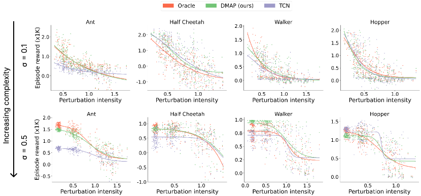
Figure F2: Reward obtained by Oracle, TCN and DMAP, trained in the $\sigma=0.1$ and $\sigma=0.5$ environments, on a wide range of perturbations (both IID and OOD). Each point represents the average reward across 5 random seeds for one body configuration, while the perturbation intensity is the eucledian norm of the perturbation vector. The curves are obtained by fitting a sigmoid function. DMAP matches or even surpasses the Oracle performance and outperform TCN (except for Hopper with $\sigma=0.5$) for all training environments.

We also show the graphs of the reward as a function for different perturbation intensity for the end-to-end trained Oracle, DMAP and TCN (Figure F2). This complements Figure 5 in the main text for $\sigma=0.3$. Generally, DMAP performs similarly to the Oracle, while the TCN has lower performance especially for more challenging morphologies (Ant, Walker).

Finally, we visualize the distribution of the IID and OOD episode rewards for different test morphologies for DMAP and TCN. To compare morphologies that might reach different rewards, we normalized the episode reward by the Oracle reward for each morphology (Figures F3 and F4). This highlights training challenges for the TCN on specific IID test morphologies (Figures F3), and that DMAP generalizes better than TCN to OOD test morphologies (Figure F4).

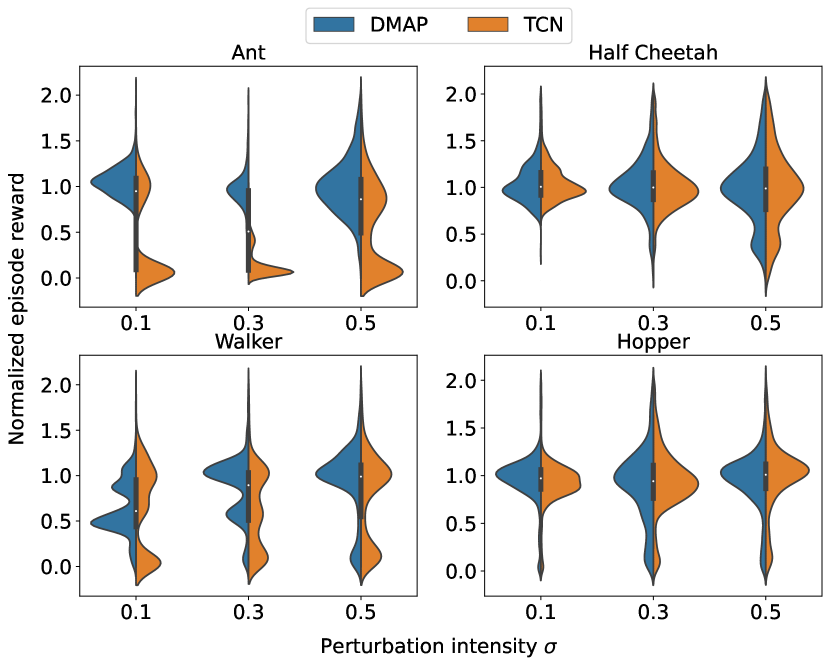
Figure F3: The normalized cumulative episode reward collected in each of the 100 test body configurations (IID test) by TCN and DMAP. Normalization was done based on Oracle rewards per morphology. We can observe that the low reward obtained by TCN in Ant and Walker is due to the density peaks in the lower part of the graphs, corresponding to agents trained with random seeds, which did not lead to a successful outcome.

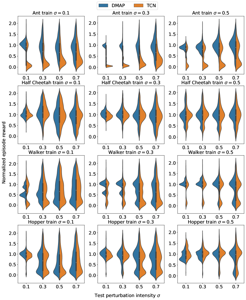
Figure F4: As in Figure F3, but keeping the training $\sigma$ fixed, while changing the test $\sigma$. In general, as the perturbation level increases, the distributions become less concentrated, because the variance of the relative performance increases. However, this suggests that OOD performance of the Oracle is a poor indicator for the generalization complexity of a morphology.

A.5 Robustness to a single leg length perturbation

To quantify the robustness of DMAP to a specific morphological perturbation, we performed an experiment where we progressively change the length of a limb in the ant (from 0 % perturbation intensity, which is the normal limb, to 100 %, which corresponds to limb amputation). We investigated how it affects the episode reward.

We found that the reward monotonically decreases, with a similar decay independent which limb is perturbed (Figure F5). Furthermore, we found an increase in robustness when DMAP is trained with higher perturbation intensity (Figure F5).

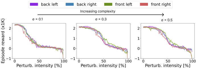
Figure F5: Reward obtained by DMAP when the length of a specific limb of the Ant agent is decreased until breakage (mean ± SEM across 5 random seeds). The perturbation intensity is expressed as the percentage of perturbation applied to the length of a specific limb (0 % normal limb, 50 % half of the limb length , 100 % limb amputation). Each color represents a different limb.

A.6 Adaptation speed to new morphological perturbation

One distinctive characteristic of RMA [15] is the short time it requires to perform motor adaptation to perturbations. We sought to compare the adaptation speed for RMA and DMAP. We could not perform online changes of the morphological parameters within an episode in PyBullet, therefore we compared speeds of RMA and DMAP when starting to run from the resting position with an unseen morphology in the Ant environment throughout all test episodes. We define the average speed as the norm of the projection of the velocity vector of the agent’s center of mass on the running surface and, since it varies during one gait cycle, we average it over a window of 30 transitions. We find that for all perturbation intensities DMAP and RMA reach the final speed after a similar number of timesteps (Figure F6). This analysis suggests that the difference in the training procedure (imitation of the Oracle’s encoder for RMA, end-to-end for DMAP) does not lead to a relevant changes in adaptation speed. Furthermore, it shows that DMAP can also rapidly adapt.

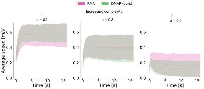
Figure F6: Average speed using the Ant agent across seeds and IID test body perturbations for different perturbation intensities. The adaptation speed to new morphological perturbation, i.e. time to reach asymptotic speed, is equivalent for RMA and DMAP.

A.7 Analysis of the attentional dynamics

When we analyzed the attentional dynamics, we found rotational dynamics (Figure 7A) and less tangling of the attentional dynamics than of the observation or action spaces for a few (randomly selected) episodes of the ant (Figure 7B). We quantified the tangling of a trajectory with the measure introduced by Russo et al. [56]:

$$Q(t)=\max_{t^{{}^{\prime}}}\frac{||\dot{x_{t}}-\dot{x_{t^{{}^{\prime}}}}||^{2}}{||x_{t}-x_{t^{{}^{\prime}}}||^{2}+\epsilon},$$

where $x_{t}$ represents the trajectory at a specific time and $x_{t^{{}^{\prime}}}$ denotes the corresponding temporal derivative, and $\epsilon$ is a constant. We use this measure to study the the difference in trajectory tangling between attention and action/observation embeddings.

Here we quantified tangling for all four environments and IID test episodes. (Figure F7). Just like for the examples in the main text, we found that the attentional dynamics are less tangled than the inputs. This suggests that DMAP achieves control across morphological parameters by regularizing the dynamics.

To gain further insights into this mechanism, we verified if the attentional dynamics become less entangled during learning. Thus, we visualized how the attentional dynamics evolve throughout the reinforcement learning (Figure F8). While at an early stage the characteristic rotational dynamics are absent, it emerges as the training proceeds, progressively untangling the trajectories.

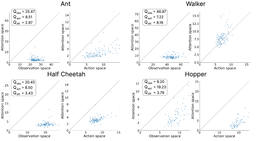
Figure F7: Scatter plot of the tangling measure for the attention embedding trajectories versus the observation and action ones. Each point represents the tangling measure for one of the 100 test body configurations averaged over time. The data refer to all the environments with $\sigma=0.1$ and to the corresponding IID test body configurations. The large majority of the points lie below the threshold line, strongly suggesting that the attention trajectories are less tangled than those of the input actions and observations. This was also observed for larger perturbation intensities.

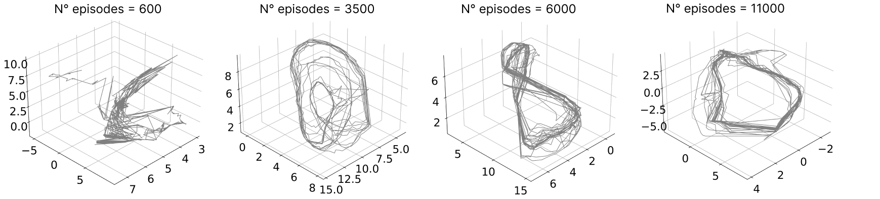
Figure F8: UMAP embedding of the attention matrix $K_{t}$ of a single training episode for different checkpoints during the training of an agent in the Ant environment with $\sigma=0.1$. The training episode is indicated in the title. The characteristic rotational dynamics emerges as the agent learns how to walk.

References

- Biewener and Patek [2018] Andrew Biewener and Sheila Patek. Animal locomotion. Oxford University Press, 2018.
- Dickinson et al. [2000] Michael H Dickinson, Claire T Farley, Robert J Full, MAR Koehl, Rodger Kram, and Steven Lehman. How animals move: an integrative view. science, 288(5463):100–106, 2000.
- Leurs et al. [2011] Françoise Leurs, Yuri P Ivanenko, Ana Bengoetxea, Ana-Maria Cebolla, Bernard Dan, Francesco Lacquaniti, and Guy A Cheron. Optimal walking speed following changes in limb geometry. Journal of Experimental Biology, 214(13):2276–2282, 2011.
- Gonçalves et al. [2022] Ana I Gonçalves, Jacob A Zavatone-Veth, Megan R Carey, and Damon A Clark. Parallel locomotor control strategies in mice and flies. Current Opinion in Neurobiology, 73:102516, 2022.
- Leiras et al. [2022] Roberto Leiras, Jared M Cregg, and Ole Kiehn. Brainstem circuits for locomotion. Annual review of neuroscience, 45, 2022.
- Wittlinger et al. [2006] Matthias Wittlinger, Rüdiger Wehner, and Harald Wolf. The ant odometer: stepping on stilts and stumps. science, 312(5782):1965–1967, 2006.
- Brockman et al. [2016] Greg Brockman, Vicki Cheung, Ludwig Pettersson, Jonas Schneider, John Schulman, Jie Tang, and Wojciech Zaremba. Openai gym. arXiv preprint arXiv:1606.01540, 2016.
- Penfield and Boldrey [1937] Wilder Penfield and Edwin Boldrey. Somatic motor and sensory representation in the cerebral cortex of man as studied by electrical stimulation. Brain, 60(4):389–443, 1937.
- Matthews [1981] Peter BC Matthews. Muscle spindles: their messages and their fusimotor supply. Handbook of physiology: I. The nervous system. American Physiological Society.[AGF], 1981.
- Shadmehr and Krakauer [2008] Reza Shadmehr and John W Krakauer. A computational neuroanatomy for motor control. Experimental brain research, 185(3):359–381, 2008.
- Azim and Seki [2019] Eiman Azim and Kazuhiko Seki. Gain control in the sensorimotor system. Current opinion in physiology, 8:177–187, 2019.
- Lindsay [2020] Grace W Lindsay. Attention in psychology, neuroscience, and machine learning. Frontiers in computational neuroscience, page 29, 2020.
- Maravita and Iriki [2004] Angelo Maravita and Atsushi Iriki. Tools for the body (schema). Trends in cognitive sciences, 8(2):79–86, 2004.
- Wolpert and Flanagan [2016] Daniel M Wolpert and J Randall Flanagan. Computations underlying sensorimotor learning. Current opinion in neurobiology, 37:7–11, 2016.
- Kumar et al. [2021] Ashish Kumar, Zipeng Fu, Deepak Pathak, and Jitendra Malik. Rma: Rapid motor adaptation for legged robots. arXiv preprint arXiv:2107.04034, 2021.
- Kirk et al. [2021] Robert Kirk, Amy Zhang, Edward Grefenstette, and Tim Rocktäschel. A survey of generalisation in deep reinforcement learning. arXiv preprint arXiv:2111.09794, 2021.
- Bellemare et al. [2013] Marc G Bellemare, Yavar Naddaf, Joel Veness, and Michael Bowling. The arcade learning environment: An evaluation platform for general agents. Journal of Artificial Intelligence Research, 47:253–279, 2013.
- Duan et al. [2016] Yan Duan, John Schulman, Xi Chen, Peter L Bartlett, Ilya Sutskever, and Pieter Abbeel. Rl2: Fast reinforcement learning via slow reinforcement learning. arXiv preprint arXiv:1611.02779, 2016.
- Machado et al. [2018] Marlos C Machado, Marc G Bellemare, Erik Talvitie, Joel Veness, Matthew Hausknecht, and Michael Bowling. Revisiting the arcade learning environment: Evaluation protocols and open problems for general agents. Journal of Artificial Intelligence Research, 61:523–562, 2018.
- Zhao et al. [2019] Chenyang Zhao, Olivier Sigaud, Freek Stulp, and Timothy M Hospedales. Investigating generalisation in continuous deep reinforcement learning. arXiv preprint arXiv:1902.07015, 2019.
- Crosby et al. [2020] Matthew Crosby, Benjamin Beyret, Murray Shanahan, José Hernández-Orallo, Lucy Cheke, and Marta Halina. The animal-ai testbed and competition. NeurIPS 2019 competition and demonstration track, pages 164–176, 2020.
- Cobbe et al. [2020] Karl Cobbe, Chris Hesse, Jacob Hilton, and John Schulman. Leveraging procedural generation to benchmark reinforcement learning. International conference on machine learning, pages 2048–2056, 2020.
- Fortunato et al. [2019] Meire Fortunato, Melissa Tan, Ryan Faulkner, Steven Hansen, Adrià Puigdomènech Badia, Gavin Buttimore, Charles Deck, Joel Z Leibo, and Charles Blundell. Generalization of reinforcement learners with working and episodic memory. Advances in Neural Information Processing Systems, 32, 2019.
- Mann et al. [2021] Khushdeep Singh Mann, Steffen Schneider, Alberto Chiappa, Jin Hwa Lee, Matthias Bethge, Alexander Mathis, and Mackenzie W Mathis. Out-of-distribution generalization of internal models is correlated with reward. Self-Supervision for Reinforcement Learning Workshop-ICLR 2021, 2021.
- Tobin et al. [2017] Josh Tobin, Rachel Fong, Alex Ray, Jonas Schneider, Wojciech Zaremba, and Pieter Abbeel. Domain randomization for transferring deep neural networks from simulation to the real world. 2017 IEEE/RSJ international conference on intelligent robots and systems (IROS), pages 23–30, 2017.
- Sadeghi and Levine [2016] Fereshteh Sadeghi and Sergey Levine. Cad2rl: Real single-image flight without a single real image. arXiv preprint arXiv:1611.04201, 2016.
- Peng et al. [2018] Xue Bin Peng, Marcin Andrychowicz, Wojciech Zaremba, and Pieter Abbeel. Sim-to-real transfer of robotic control with dynamics randomization. 2018 IEEE international conference on robotics and automation (ICRA), pages 3803–3810, 2018.
- Yu et al. [2017] Wenhao Yu, Jie Tan, C Karen Liu, and Greg Turk. Preparing for the unknown: Learning a universal policy with online system identification. arXiv preprint arXiv:1702.02453, 2017.
- Wang et al. [2016] Jane X Wang, Zeb Kurth-Nelson, Dhruva Tirumala, Hubert Soyer, Joel Z Leibo, Remi Munos, Charles Blundell, Dharshan Kumaran, and Matt Botvinick. Learning to reinforcement learn. arXiv preprint arXiv:1611.05763, 2016.
- Fujimoto et al. [2018] Scott Fujimoto, Herke Hoof, and David Meger. Addressing function approximation error in actor-critic methods. International conference on machine learning, pages 1587–1596, 2018.
- Haarnoja et al. [2018] Tuomas Haarnoja, Aurick Zhou, Pieter Abbeel, and Sergey Levine. Soft actor-critic: Off-policy maximum entropy deep reinforcement learning with a stochastic actor. International conference on machine learning, pages 1861–1870, 2018.
- Raffin et al. [2022] Antonin Raffin, Jens Kober, and Freek Stulp. Smooth exploration for robotic reinforcement learning. Conference on Robot Learning, pages 1634–1644, 2022.
- Kapturowski et al. [2018] Steven Kapturowski, Georg Ostrovski, John Quan, Remi Munos, and Will Dabney. Recurrent experience replay in distributed reinforcement learning. International conference on learning representations, 2018.
- Hospedales et al. [2021] Timothy Hospedales, Antreas Antoniou, Paul Micaelli, and Amos Storkey. Meta-learning in neural networks: A survey. IEEE transactions on pattern analysis and machine intelligence, 44(9):5149–5169, 2021.
- Nagabandi et al. [2018a] Anusha Nagabandi, Ignasi Clavera, Simin Liu, Ronald S Fearing, Pieter Abbeel, Sergey Levine, and Chelsea Finn. Learning to adapt in dynamic, real-world environments through meta-reinforcement learning. arXiv preprint arXiv:1803.11347, 2018a.
- Nagabandi et al. [2018b] Anusha Nagabandi, Chelsea Finn, and Sergey Levine. Deep online learning via meta-learning: Continual adaptation for model-based rl. arXiv preprint arXiv:1812.07671, 2018b.
- Rakelly et al. [2019] Kate Rakelly, Aurick Zhou, Chelsea Finn, Sergey Levine, and Deirdre Quillen. Efficient off-policy meta-reinforcement learning via probabilistic context variables. pages 5331–5340. PMLR, 2019.
- Pathak et al. [2019] Deepak Pathak, Christopher Lu, Trevor Darrell, Phillip Isola, and Alexei A Efros. Learning to control self-assembling morphologies: a study of generalization via modularity. Advances in Neural Information Processing Systems, 32, 2019.
- Whitman et al. [2021] Julian Whitman, Matthew Travers, and Howie Choset. Learning modular robot control policies. arXiv preprint arXiv:2105.10049, 2021.
- Wang et al. [2018] Tingwu Wang, Renjie Liao, Jimmy Ba, and Sanja Fidler. Nervenet: Learning structured policy with graph neural networks. International conference on learning representations, 2018.
- Huang et al. [2020] Wenlong Huang, Igor Mordatch, and Deepak Pathak. One policy to control them all: Shared modular policies for agent-agnostic control. International Conference on Machine Learning, pages 4455–4464, 2020.
- Kurin et al. [2020] Vitaly Kurin, Maximilian Igl, Tim Rocktäschel, Wendelin Boehmer, and Shimon Whiteson. My body is a cage: the role of morphology in graph-based incompatible control. arXiv preprint arXiv:2010.01856, 2020.
- Trabucco et al. [2022] Brandon Trabucco, Mariano Phielipp, and Glen Berseth. Anymorph: Learning transferable polices by inferring agent morphology. pages 21677–21691. PMLR, 2022.
- Pateria et al. [2021] Shubham Pateria, Budhitama Subagdja, Ah-hwee Tan, and Chai Quek. Hierarchical reinforcement learning: A comprehensive survey. ACM Computing Surveys (CSUR), 54(5):1–35, 2021.
- Levy et al. [2017] Andrew Levy, Robert Platt, and Kate Saenko. Hierarchical actor-critic. arXiv preprint arXiv:1712.00948, 12, 2017.
- Rao et al. [2021] Dushyant Rao, Fereshteh Sadeghi, Leonard Hasenclever, Markus Wulfmeier, Martina Zambelli, Giulia Vezzani, Dhruva Tirumala, Yusuf Aytar, Josh Merel, Nicolas Heess, et al. Learning transferable motor skills with hierarchical latent mixture policies. arXiv preprint arXiv:2112.05062, 2021.
- Li et al. [2019] Alexander C Li, Carlos Florensa, Ignasi Clavera, and Pieter Abbeel. Sub-policy adaptation for hierarchical reinforcement learning. arXiv preprint arXiv:1906.05862, 2019.
- Coumans and Bai [2016–2019] Erwin Coumans and Yunfei Bai. Pybullet, a python module for physics simulation for games, robotics and machine learning. http://pybullet.org, 2016–2019.
- Raffin [2018] Antonin Raffin. Rl baselines zoo. https://github.com/araffin/rl-baselines-zoo, 2018.
- Liang et al. [2018] Eric Liang, Richard Liaw, Robert Nishihara, Philipp Moritz, Roy Fox, Ken Goldberg, Joseph Gonzalez, Michael Jordan, and Ion Stoica. Rllib: Abstractions for distributed reinforcement learning. International Conference on Machine Learning, pages 3053–3062, 2018.
- McInnes et al. [2020] Leland McInnes, John Healy, and James Melville. Umap: uniform manifold approximation and projection for dimension reduction. 2020.
- Holmes et al. [2006] Philip Holmes, Robert J Full, Dan Koditschek, and John Guckenheimer. The dynamics of legged locomotion: Models, analyses, and challenges. SIAM review, 48(2):207–304, 2006.
- Hoogkamer et al. [2015] Wouter Hoogkamer, Frank Van Calenbergh, Stephan P Swinnen, and Jacques Duysens. Cutaneous reflex modulation and self-induced reflex attenuation in cerebellar patients. Journal of Neurophysiology, 113(3):915–924, 2015.
- Zador [2019] Anthony M Zador. A critique of pure learning and what artificial neural networks can learn from animal brains. Nature communications, 10(1):1–7, 2019.
- Royakkers and van Est [2015] Lambèr Royakkers and Rinie van Est. A literature review on new robotics: automation from love to war. International journal of social robotics, 7(5):549–570, 2015.
- Russo et al. [2018] Abigail A Russo, Sean R Bittner, Sean M Perkins, Jeffrey S Seely, Brian M London, Antonio H Lara, Andrew Miri, Najja J Marshall, Adam Kohn, Thomas M Jessell, et al. Motor cortex embeds muscle-like commands in an untangled population response. Neuron, 97(4):953–966, 2018.